Influenza Neuraminidase Inhibitor IC50 Data:Calculation, Interpretation and Statistical Analyses

Presentation Outline

• Determining IC50 values

Curve-fitting methods

Sources of variation

• Identifying IC50 outliers

Determining cut-offs/thresholds

Outlier values versus resistant viruses

• Monitoring trends over time in IC50 data

Abbreviations

NA: Neuraminidase

NI: Neuraminidase Inhibitor

RFU: Relative Fluorescence Units

RLU: Relative Luminescence Units

VC: Virus Control

Determining NI IC50 Values

IC50: The concentration of NI which reduces NA activity by 50% of the virus-control, or upper asymptote

Estimated by: Measuring the NA activity (RFU or RLU) of an isolate against a range of dilutions of the drug, as well as without drug (virus-control)

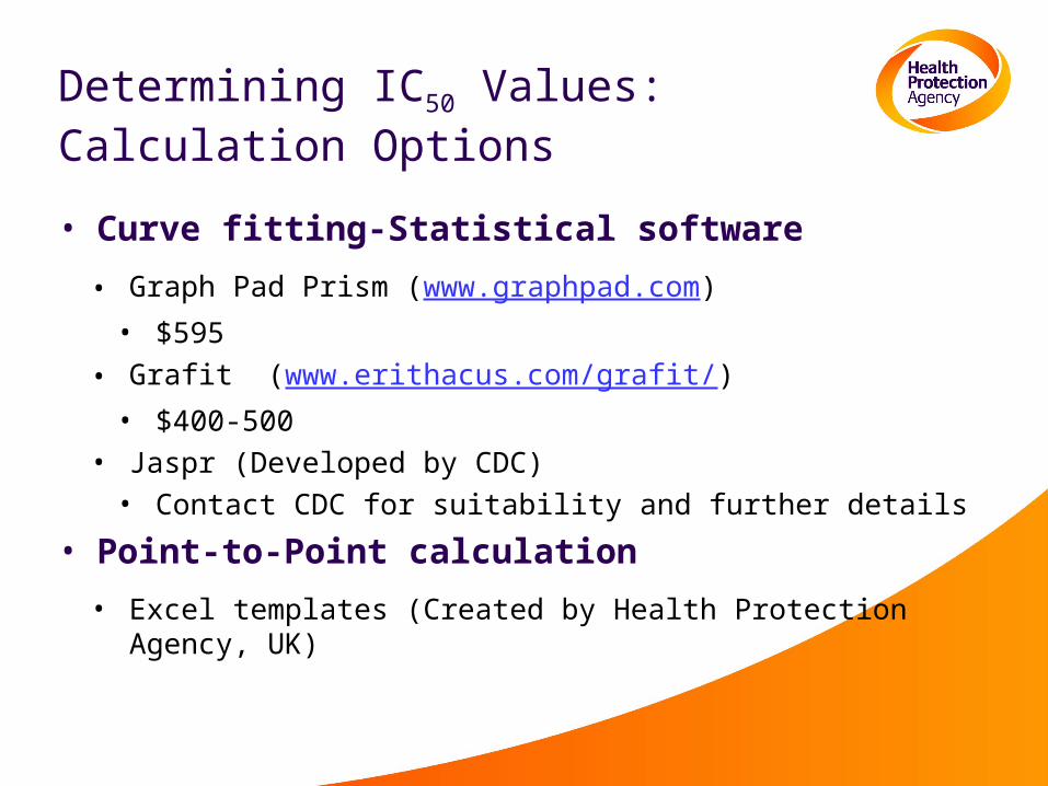
Determining IC50 Values: Calculation Options

• Curve fitting-Statistical software

• Graph Pad Prism (www.graphpad.com)• $595

• Grafit (www.erithacus.com/grafit/)• $400-500

• Jaspr (Developed by CDC)• Contact CDC for suitability and further details

• Point-to-Point calculation

• Excel templates (Created by Health Protection Agency, UK)

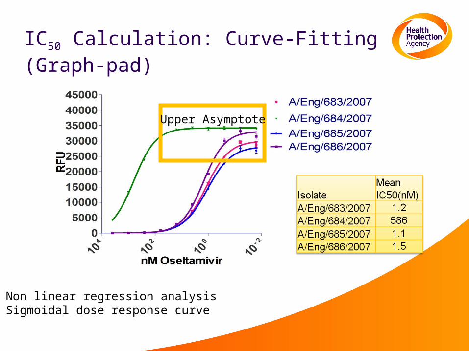
IC50 Calculation: Curve-Fitting (Graph-pad)

Upper Asymptote

Non linear regression analysisSigmoidal dose response curve

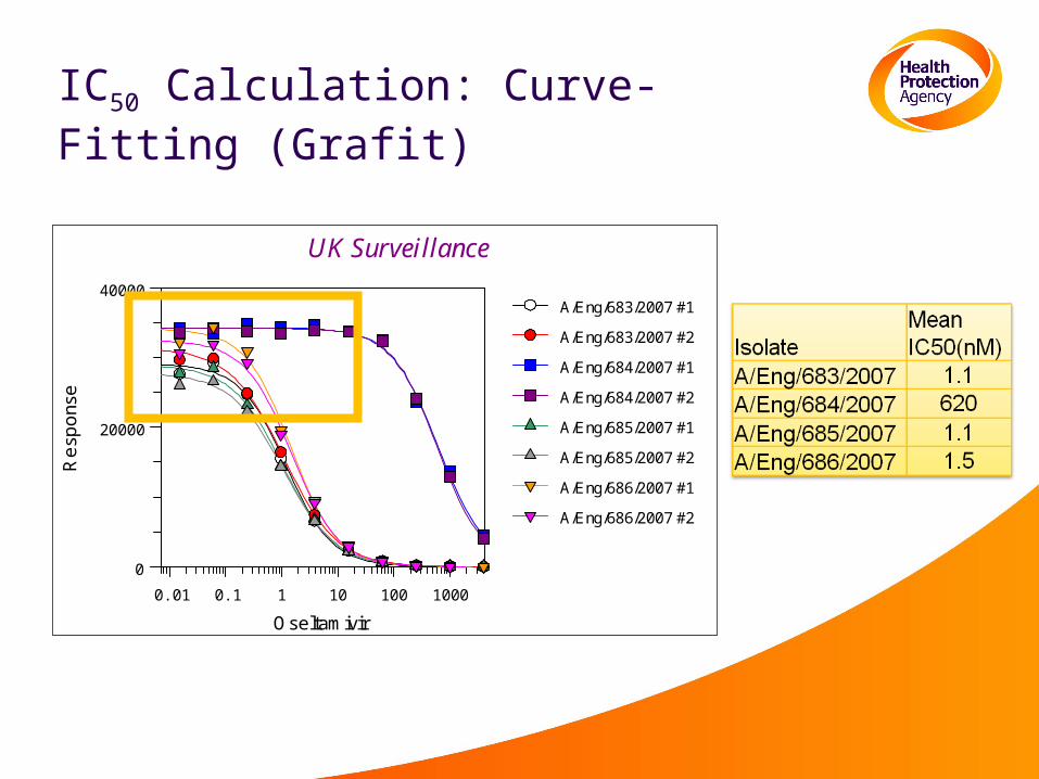
IC50 Calculation: Curve-Fitting (Grafit)

UK Surveillance

Oseltamivir

0.01 0.1 1 10 100 1000

Re

spo

nse

0

20000

40000A/Eng/683/2007 #1

A/Eng/683/2007 #2

A/Eng/684/2007 #1

A/Eng/684/2007 #2

A/Eng/685/2007 #1

A/Eng/685/2007 #2

A/Eng/686/2007 #1

A/Eng/686/2007 #2

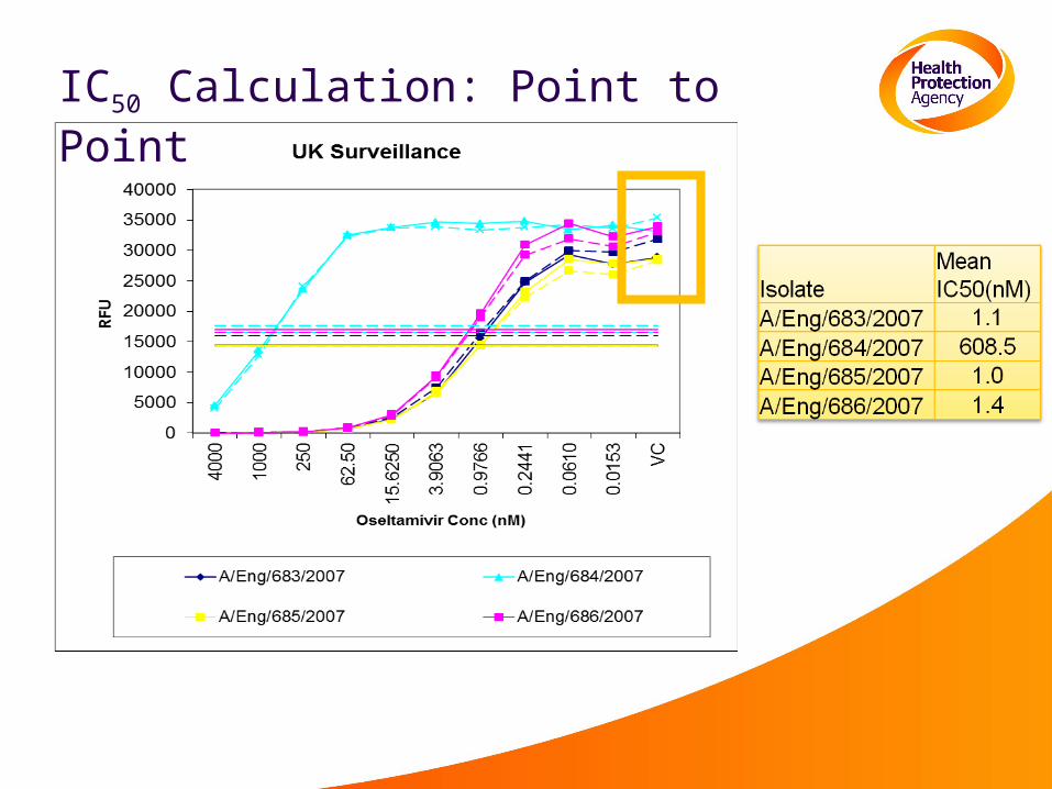
IC50 Calculation: Point to Point

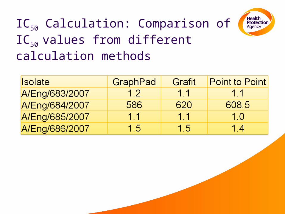
IC50 Calculation: Comparison of IC50

values from different calculation methods

• Method of calculation

• Using point-to-point or curve fitting software• Choice of curve fitting software used

• Intra-assay variation

• Difference between 2 or more replicates

• Inter-assay variation

Difference in calculated value for a given isolate in multiple assays

Determining IC50 Values: Sources of Variation

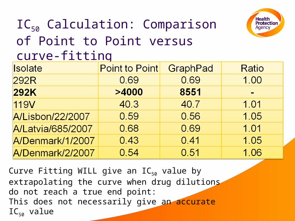
IC50 Calculation: Comparison of Point to Point versus curve-fitting

Curve Fitting WILL give an IC50 value by extrapolating the curve when drug dilutions do not reach a true end point:This does not necessarily give an accurate IC50 value

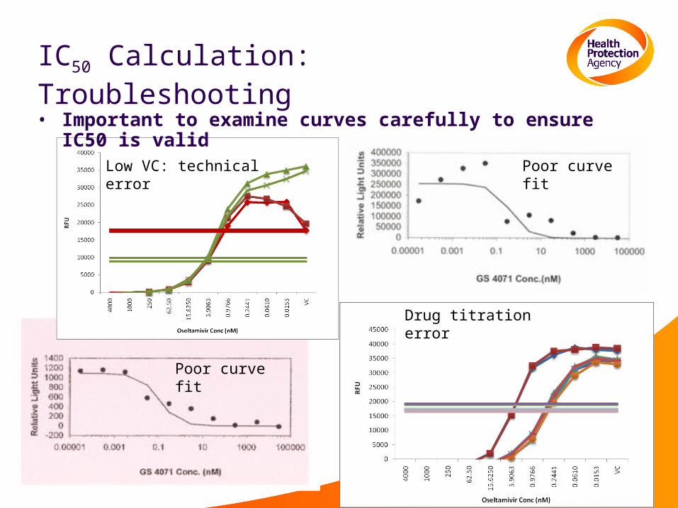
IC50 Calculation: Troubleshooting

Low VC: technical error Poor curve fit

Poor curve fit

Drug titration error

• Important to examine curves carefully to ensure IC50 is valid

Comments: Choice of IC50 Calculation Method

• Choice of IC50 calculation method will make no more than about 5% difference to IC50 value, for most samples

• Must be clear exactly how the curve fitting and calculation of IC50 is working

• Is IC50 based on 50% of RFU/RLU of VC or 50% of fitted upper asymptote.

• Regardless of method used, careful examination of the curve produced is required to identify technical issues.

• See presentation on validation and troubleshooting of IC50 testing methods

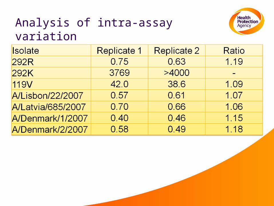
Analysis of intra-assay variation

Comments: Intra-assay Variation

• Variation between replicates in the same assay can be 15%-20%.

• This variation is greater than that seen with changes to curve-fitting method

• Using replicates and taking the average reduces this effect.

• A large difference between replicates (e.g. >30%) of a given virus indicates a technical issue

• In these instances repeat testing should be performed

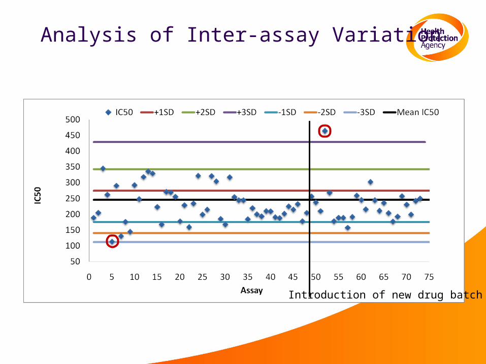
Analysis of Inter-assay Variation

Introduction of new drug batch

Analysis of Inter-assay Variation

Comments: Inter-assay Variation

• Variation in IC50 values for a virus in multiple assays can be 50%.

• Control viruses should be included in every assay to identify technical issues.

• Control viruses should be validated, and have a defined range between which the IC50 is valid.

• Assays in which the control virus IC50 falls outside the accepted range should be reaped in their entirety.

Conclusions: Determining IC50 Values

• Several methods for IC50 calculation available at a range of price and sophistication

• Variation due to choice of IC50 calculation method is minimal (5-10%) in comparison with intra-assay (20%) and inter-assay (50%) variation.

• Choice of curve-fitting method should be made based on individual laboratory circumstances

• All variation can be minimised using appropriate assay controls (reference/control viruses, validation of curves generated)

• Consistency in methodology used (statistical and laboratory) is important for long term analysis (time trends)

Identifying IC50 outliers

• Aim: identify isolates with higher (or lower) than expected IC50 values (outliers)

• First determine the ‘normal range’ of IC50 values

• Each

• Various statistical methods may be used

• Critical to ensure that any outliers do not unduly affect the cut-off/threshold

• Outlier does not equal resistant

• Identifies isolates that may be worth further investigation (retesting/sequencing)

Identifying IC50 outliers: Commonly Used Statistical Methods

• SMAD

Robust estimate of the standard deviation based on the median absolute deviation from the median

• Box and Whisker plots

Graphical representation of the 5 number summary of the data (the sample minimum, the lower or first quartile, the median, the upper or third quartile, the sample maximum)

• Both methods require a minimum dataset to perform robust analyses (>20)

• Cut offs can be calculated mid-season, once a reasonable number of samples has been tested, to monitor outliers

• At the end of the season, cut offs can be updated and a retrospective analysis of all season data performed.

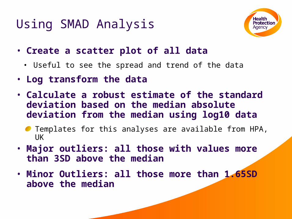
Using SMAD Analysis

• Create a scatter plot of all data

• Useful to see the spread and trend of the data

• Log transform the data

• Calculate a robust estimate of the standard deviation based on the median absolute deviation from the median using log10 data

Templates for this analyses are available from HPA, UK

• Major outliers: all those with values more than 3SD above the median

• Minor Outliers: all those more than 1.65SD above the median

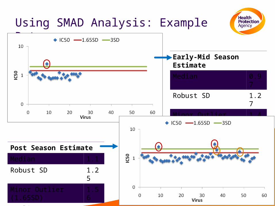
Using SMAD Analysis: Example Data

Early-Mid Season Estimate

Median 0.97

Robust SD 1.27

Minor Outlier (1.65SD) 1.45

Outlier (3SD) 1.99

Post Season Estimate

Median 1.1

Robust SD 1.25

Minor Outlier (1.65SD) 1.56

Outlier (3SD) 2.11

Using Box and Whisker Analysis

• This analysis can be performed in Graphpad Prism, with the box and whisker plots drawn automatically

• Calculations can be done in excel, but drawing the box and whisker plots is more complicated

A template for plotting the graphs is available from Adam Meijer

• Log transform the data

• Calculate the median, upper quartile, lower quartile, interquartile range, upper minor and major fences, and lower major and minor fences

• Mild outliers lie between the minor and major fences

• Extreme outliers lie outside the major fence

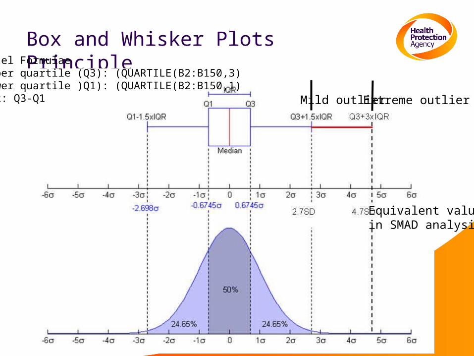
Box and Whisker Plots Principle

Mild outlier Extreme outlier

Equivalent valuesin SMAD analysis

Excel FormulaeUpper quartile (Q3): (QUARTILE(B2:B150,3)Lower quartile )Q1): (QUARTILE(B2:B150,1)IQR: Q3-Q1

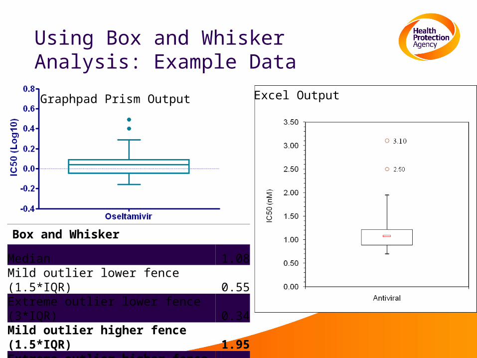
Using Box and Whisker Analysis: Example Data

Box and Whisker

Median 1.08

Mild outlier lower fence (1.5*IQR) 0.55

Extreme outlier lower fence (3*IQR) 0.34

Mild outlier higher fence (1.5*IQR) 1.95

Extreme outlier higher fence (3*IQR) 3.14

Graphpad Prism Output Excel Output

Do we need to log-transform?

• Most results from dilution assays produce ‘geometric results’ so likely to be sensible

• Sometimes data are skewed. (e.g. lower quartile much closer to median than upper quartile)

• Important to log transform as robust methods assume data are normal once outliers are removed.

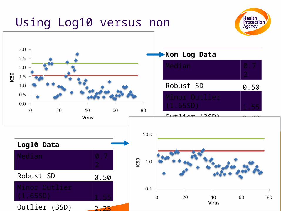
Using Log10 versus non logged Data

Non Log Data

Median 0.72

Robust SD 0.50

Minor Outlier (1.65SD) 1.55

Outlier (3SD) 2.23

Log10 Data

Median 0.72

Robust SD 0.50

Minor Outlier (1.65SD) 1.55

Outlier (3SD) 2.23

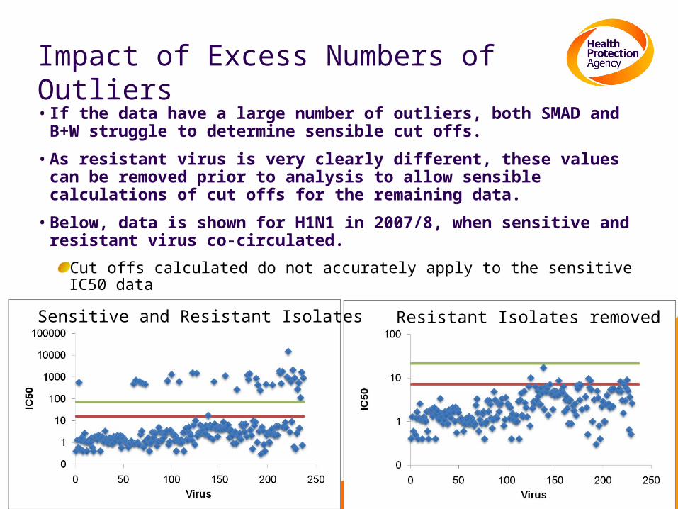
Impact of Excess Numbers of Outliers

• If the data have a large number of outliers, both SMAD and B+W struggle to determine sensible cut offs.

• As resistant virus is very clearly different, these values can be removed prior to analysis to allow sensible calculations of cut offs for the remaining data.

• Below, data is shown for H1N1 in 2007/8, when sensitive and resistant virus co-circulated.

Cut offs calculated do not accurately apply to the sensitive IC50 data

Resistant Isolates removedSensitive and Resistant Isolates

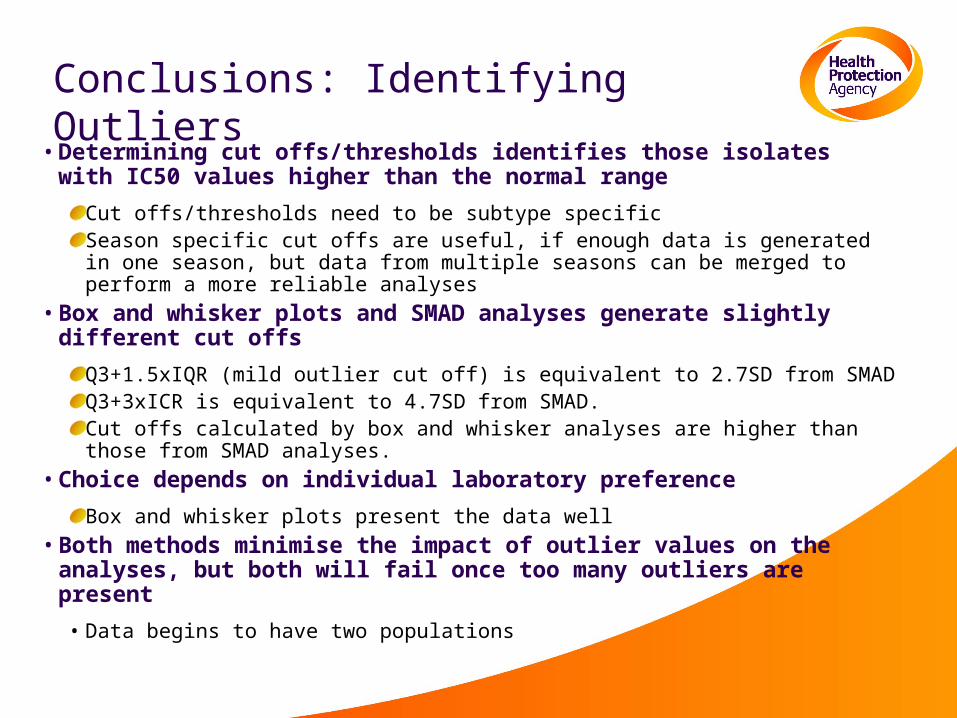
Conclusions: Identifying Outliers

• Determining cut offs/thresholds identifies those isolates with IC50 values higher than the normal range

Cut offs/thresholds need to be subtype specificSeason specific cut offs are useful, if enough data is generated in one season, but data from multiple seasons can be merged to perform a more reliable analyses

• Box and whisker plots and SMAD analyses generate slightly different cut offs

Q3+1.5xIQR (mild outlier cut off) is equivalent to 2.7SD from SMADQ3+3xICR is equivalent to 4.7SD from SMAD. Cut offs calculated by box and whisker analyses are higher than those from SMAD analyses.

• Choice depends on individual laboratory preference

Box and whisker plots present the data well

• Both methods minimise the impact of outlier values on the analyses, but both will fail once too many outliers are present

• Data begins to have two populations

Monitoring Trends Over Time

• The normal range of IC50 values for a particular subtype can change over time

• This could be seen by an increase in the number of outliers, or by changes in the median

• Simple to monitor, using the methods already described for identifying outliers

• scatter plots/box-whisker

• Other statistical methods can be used to further analyse data from several seasons

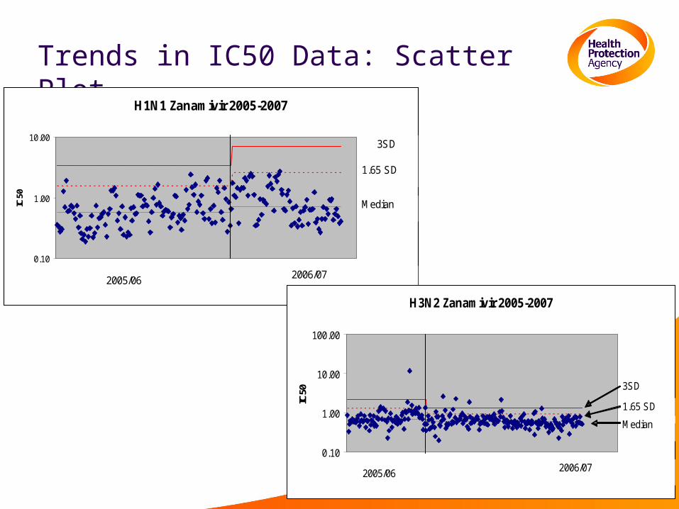
Trends in IC50 Data: Scatter Plot

H1N1 Zanamivir 2005-2007

0.10

1.00

10.00

IC50

2005/06 2006/07

3SD

1.65 SD

Median

H3N2 Zanamivir 2005-2007

0.10

1.00

10.00

100.00

IC50

2005/06 2006/07

3SD

1.65 SD

Median

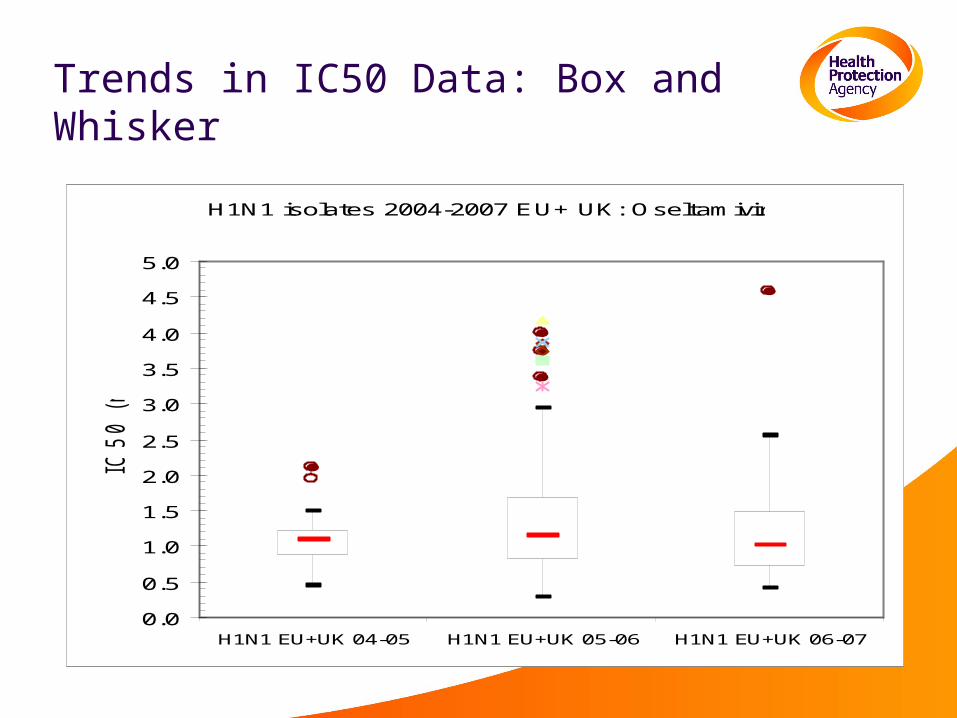
Trends in IC50 Data: Box and Whisker

H1N1 isolates 2004-2007 EU+ UK: Oseltamivir

0.0

0.5

1.0

1.5

2.0

2.5

3.0

3.5

4.0

4.5

5.0

H1N1 EU+UK 04-05 H1N1 EU+UK 05-06 H1N1 EU+UK 06-07

IC50 (

nM

)

Summary

• Good use of statistical methods can help interpret the IC50 results and ensure assay results are reliable.

• Analyses of data not only identifies individual outliers, but allows continuous monitoring of trends

• Retrospective analyses of multiple seasons of data can identify changes in viral characteristics and susceptibilities

• Do not use statistics without first looking at the data by scatter plot to find obvious deviations which require an adapted statistical approach

• Challenge is to find explanations for trends