IASI carbon monoxide validation over the Arctic during ... · M. Pommier et al.: IASI carbon monoxide validation over the Arctic 10657 Sect. 3. Section 4 describes the collocation

Atmos. Chem. Phys., 10, 10655–10678, 2010www.atmos-chem-phys.net/10/10655/2010/doi:10.5194/acp-10-10655-2010© Author(s) 2010. CC Attribution 3.0 License.

AtmosphericChemistry

and Physics

IASI carbon monoxide validation over the Arctic duringPOLARCAT spring and summer campaigns

M. Pommier1, K. S. Law1, C. Clerbaux1,3, S. Turquety2, D. Hurtmans3, J. Hadji-Lazaro1, P.-F. Coheur3, H. Schlager4,G. Ancellet1, J.-D. Paris5, P. Nedelec6, G. S. Diskin7, J. R. Podolske8, J. S. Holloway9,10, and P. Bernath11,12

1UPMC Univ. Paris 06, Universite Versailles St-Quentin, CNRS/INSU, UMR 8190, LATMOS-IPSL, Paris, France2UPMC Univ. Paris 06, Ecole Polytechnique, CNRS UMR 8539, LMD-IPSL, Palaiseau, France3Spectroscopie de l’Atmosphere, Chimie Quantique et Photophysique, Universite Libre de Bruxelles (ULB),Brussels, Belgium4DLR, Institut fur Physik der Atmosphare, Oberpfaffenhofen, Germany5LSCE/IPSL, CEA-CNRS-UVSQ, Saclay, France6Universite de Toulouse, UPS, LA (Laboratoire d’Aerologie), CNRS UMR 5560, Toulouse, France7NASA Langley Research Center, MS 483, Hampton, USA8NASA Ames Research Center, Moffett Field, California, 94035, USA9Chemical Sciences Division, NOAA Earth System Research Laboratory, Boulder, Colorado, USA10Cooperative Institute for Research in Environmental Sciences, University of Colorado, Boulder, Colorado, USA11Department of Chemistry, University of Waterloo, Waterloo, Ontario, Canada N2L 3G1, Canada12Department of Chemistry, University of York, Heslington, York YO10 5DD, UK

Received: 22 April 2010 – Published in Atmos. Chem. Phys. Discuss.: 9 June 2010Revised: 7 October 2010 – Accepted: 8 November 2010 – Published: 12 November 2010

Abstract. In this paper, we provide a detailed com-parison between carbon monoxide (CO) data measuredby the Infrared Atmospheric Sounding Interferometer(IASI)/MetOp and aircraft observations over the Arctic.The CO measurements were obtained during North Ameri-can (NASA ARCTAS and NOAA ARCPAC) and Europeancampaigns (POLARCAT-France, POLARCAT-GRACE andYAK-AEROSIB) as part of the International Polar Year(IPY) POLARCAT activity in spring and summer 2008. Dur-ing the campaigns different air masses were sampled in-cluding clean air, polluted plumes originating from anthro-pogenic sources in Europe, Asia and North America, and for-est fire plumes originating from Siberia and Canada. The pa-per illustrates that CO-rich plumes following different trans-port pathways were well captured by the IASI instrument,in particular due to the high spatial coverage of IASI. Thecomparison between IASI CO total columns, 0–5 km par-tial columns and profiles with collocated aircraft data wasachieved by taking into account the different sensitivity andgeometry of the sounding instruments. A detailed analysis

Correspondence to:M. Pommier([email protected])

is provided and the agreement is discussed in terms of in-formation content and surface properties at the location ofthe observations. For profiles, the data were found to be ingood agreement in spring with differences lower than 17%,whereas in summer the difference can reach 20% for IASIprofiles below 8 km for polluted cases. For total columns thecorrelation coefficients ranged from 0.15 to 0.74 (from 0.47to 0.77 for partial columns) in spring and from 0.26 to 0.84(from 0.66 to 0.88 for partial columns) in summer. A betteragreement is seen over the sea in spring (0.73 for total col-umn and 0.78 for partial column) and over the land in sum-mer (0.69 for total columns and 0.81 for partial columns).The IASI vertical sensitivity was better over land than oversea, and better over land than over sea ice and snow allowinga higher potential to detect CO vertical distribution duringsummer.

1 Introduction

The Arctic atmosphere is a natural receptor of pollution fromthe continents of the Northern Hemisphere. The Arctic tro-posphere was believed to be extremely clean until the 1950swhen flights above the Canadian and Alaskan Arctic went

Published by Copernicus Publications on behalf of the European Geosciences Union.

http://creativecommons.org/licenses/by/3.0/

10656 M. Pommier et al.: IASI carbon monoxide validation over the Arctic

through strong haze, decreasing the visibility (Greenaway,1950; Mitchell, 1957). This so-called “Arctic Haze” is a re-curring phenomenon that has been observed every winter andspring. The origin of this pollution is long-range transportof aerosols and accumulation of persistent pollutants such asmercury and ozone (O3). Recent studies (e.g. Shindell et al.,2008; Stohl, 2006) show that the Arctic troposphere is influ-enced, according to the season, by emissions from Europe,North America or Asia. These pollutants originate from largeurban areas, as well as from boreal fires. Atmospheric pollu-tion in this region may be having an effect on human healthand also on climate through direct radiative effects or indi-rect effects such as enhanced summer sea-ice melt resultingfrom deposition of black carbon aerosols on snow and ice(Law and Stohl, 2007). Tropospheric ozone, an importantgreenhouse gas, could contribute, according to model simu-lations, to about 0.4◦C to 0.5◦C of winter and spring Arc-tic warming (Shindell et al., 2006). In the free troposphere,limited measurements such as those at Summit, Greenland,show a late spring/early summer ozone maximum (Helmiget al., 2007). Ozone can either be photochemically producedin mid-latitude source regions or during transport of pollu-tion plumes to the Arctic. Transport of ozone rich-air fromthe upper troposphere or lower stratosphere is also a source.Carbon monoxide (CO) has been used in a number of studiesas a tracer of pollution transport thanks to its relatively longlifetime of several weeks in the troposphere. In addition, COis an important precursor of ozone through photochemicalproduction, in the presence of nitrogen oxides (NOx). It ismainly produced from the combustion of fossil fuels by in-dustry, car traffic or domestic heating system, and vegetationcombustion or forest fires (e.g. Badr and Probert, 1995). Itis also produced in the atmosphere following oxidation ofmethane (CH4) and non-methane hydrocarbons (NMHCs)by hydroxyl radicals (OH). Since its main sink is reactionwith OH, CO has an important role in the oxidizing powerof the atmosphere, regulating the concentrations of CH4 andO3.

In recent decades many surface and in situ measurementshave been made in the Arctic from ground stations, aircraftand balloon-borne platforms, providing observations of sev-eral trace species, including CO. Intensive field campaignsusing airborne instrumentation often measure enough speciesto allow detailed analysis of the chemical composition of theair masses. Several past campaigns have sampled pollutiontransport events such as the Arctic Boundary Layer Expedi-tion (ABLE) in 1988 (Harriss et al., 1992), the TroposphericOzone Production about the Spring Equinox (TOPSE) in2000 (Atlas et al., 2003) and the International Consortiumfor Atmospheric Research on Transport and Transforma-tion (ICARTT) in 2004 (Fehsenfeld et al., 2006). More re-cently, several aircraft campaigns were conducted in 2008in the framework of the International Polar Year (IPY) fo-cusing on pollutant transport (trace gas and aerosol), climateand Arctic tropospheric chemistry studies as part of the In-

ternational Global Atmospheric Chemistry (IGAC) activityPOLARCAT (Polar Study using Aircraft, Remote Sensing,Surface Measurements and Models, of Climate, Chemistry,Aerosols, and Transport). Observations from these aircraftcampaigns, which were collected over a period of severalweeks, provide a snapshot of Arctic chemical composition.They were complemented by satellite data which, even iftheir accuracy is lower, can provide global and continuousmonitoring of the distributions of several trace gases, includ-ing CO. Satellite data have clearly shown long-range trans-port of CO plumes between continents (Turquety et al., 2007;Rinsland et al., 2007; McMillan et al., 2008; Yurganov et al.,2008; Fisher et al., 2010).

Among the satellite sounders probing CO, the InfraredAtmospheric Sounding Interferometer (IASI) instrument,launched on board the polar-orbiting MetOp-A satellite on19 October 2006, is the first of three consecutive instrumentsto be launched on the MetOp satellites. MetOp-A has a sun-synchronous orbit with a 09:30 local equator crossing time.With 14 daily orbits and a large scanning swath of 2200 kmacross the track, IASI provides global Earth coverage twicea day, and is thus particularly well suited for the analysisof long-range transport. Moreover, its polar orbit (inclina-tion of 98.7◦) allows enhanced coverage above the polar re-gion. However, the nadir-viewing geometry implies limitedvertical resolution, typically∼6 km for CO, with one to twoindependent pieces of information on the vertical distribu-tion, depending mostly on surface temperature/thermal con-trast (George et al., 2009; Clerbaux et al., 2009).

Satellite data need to be validated against independentmeasurements. The IASI CO total columns have recentlybeen evaluated through comparisons with other satellite-borne instrument data (MOPITT, TES and AIRS) (Georgeet al., 2009) and IASI was shown to perform well comparedto other thermal infrared remote sensors. As yet, the IASIretrieved CO profiles have not been evaluated against in situobservations. In this paper, we evaluate the quality of theIASI CO data in the Arctic, taking advantage of the inten-sive aircraft campaigns as part of POLARCAT undertaken in2008. Many in situ CO profiles were collected during land-ing, take-off, pollution exploration and during specific satel-lite validation flights. Specific difficulties associated with re-trievals above the Arctic are investigated such as retrievalsover ice, satellite observations above source regions as wellas the seasonal variation of CO observations. Since theairborne observations are only performed up to∼7–12 km(depending on the aircraft capabilities), the vertical profilesretrieved from the IASI nadir radiance measurements werecompared with in situ profiles completed with a climatologybuilt using limb CO profiles for different seasons and lati-tudes.

The paper is organized as follows: after an overview ofthe IASI CO retrievals over the Arctic (Sect. 2), the gen-eral context of the 2008 polar campaigns and details aboutthe CO measurements used for the validation are given in

Atmos. Chem. Phys., 10, 10655–10678, 2010 www.atmos-chem-phys.net/10/10655/2010/

M. Pommier et al.: IASI carbon monoxide validation over the Arctic 10657

Sect. 3. Section 4 describes the collocation criteria issue andthe methodology adopted to validate IASI CO. Both a quan-titative comparison and a statistical evaluation of the qualityof the IASI CO retrievals in spring and summer 2008 areprovided. Section 5 discusses further some of the interest-ing cases in terms of the spatial distribution of the observedplumes. Conclusions are presented in Sect. 6.

2 IASI

2.1 CO retrievals

IASI is a high resolution nadir looking thermal infrared (IR)sounder. It is a Fourier Transform Spectrometer (FTS) thatrecords radiance measurements from the Earth’s surface andthe atmosphere with a high spectral resolution of 0.5 cm−1

(apodized) and spectrally sampled at 0.25 cm−1 over an ex-tended spectral range from 645 to 2760 cm−1, and with a lowradiometric noise (0.2–0.35 K at 280 K reference). Globalscale distributions of several species can be derived from theatmospheric spectra, such as CO, O3, HNO3, CH4, H2O,NH3 and other reactive trace gases (Clerbaux et al., 2009;George et al., 2009; Boynard et al., 2009; Wespes et al.,2009; Razavi et al., 2009; Herbin et al., 2009; Coheur et al.,2009; Clarisse et al., 2008). In addition, the dense horizontalcoverage due to the large swath (2200 km) and the 14 dailyorbits allow global Earth coverage twice a day, with eachview being an atmospheric cell composed of 2× 2 circularpixels each with a∼12 km footprint diameter in nadir.

IASI CO distributions are retrieved from IASI radiancespectra (2143–2181 cm−1 spectral range) using the FORLI-CO (Fast Optimal Retrievals on Layers for IASI-CO) re-trieval algorithm developed at the Universite Libre de Brux-elles (ULB) (Turquety et al., 2009; George et al., 2009). Thealgorithm is based for the retrieval on the Optimal Estima-tion Method (OEM) described by Rodgers (2000). In ad-dition to IASI spectra, the software uses the water vapourand temperature profiles from ECMWF (European Centrefor Medium-Range Weather Forecasts) as input variables orfrom IASI level 2 operational data and distributed by EU-METSAT through the EUMETCAST dissemination system(Schluessel et al., 2005) as well as surface emissivity fromthe MODIS/Terra climatology (Wan, 2008). In this study,the temperature and water vapour profiles were taken fromECMWF analyses because the IASI retrieved data were notyet available.

The FORLI-CO algorithm provides CO profiles in volumemixing ratio (vmr) or partial column on 19 layers from thesurface to the top of the atmosphere (60 km), each one kilo-metre thick, as well as error characterization diagnostics, in-cluding an a posteriori error variance-covariance matrix andan averaging kernel (AK) matrix. From these matrices ascalar error and a vector averaging kernel can be calculated,and are provided with the total column product.

The OEM seeks the optimal solution for the CO profileconsidering a given IASI radiance spectrum and the associ-ated measurement error covariance matrixSε. Since morethan one solution can fit the observations, it is necessaryto constrain the results with a priori information contain-ing both the average value expected a priori profilexa, andthe allowed variability around this average given by the so-called a priori covariance matrixSa (see Fig. 1). In orderto build a matrix representative of both background and pol-luted conditions the a priori information was constructed us-ing a database of CO profiles including aircraft profiles dur-ing landing and take-off from the MOZAIC (Measurementsof OZone and water vapour by AIrbus in-service airCraft)program (Nedelec et al., 2003), ACE-FTS satellite observa-tions in the upper troposphere and lower stratosphere (Cler-baux et al., 2005) and distributions computed by the LMDz-INCA global chemistry-transport model (e.g. Turquety et al.,2008).

The OEM solution can be found by iteratively applying:

xi+1 = xa+Dy[y −F(xi)−K i(xa− xi)] (1)

With Dy = SiKTi S−1

ε and Si+1 = (KTi+1S−1

ε K i+1 +S−1a )−1.

K i is the Jacobian at statexi , KTi is its transpose andxi+1

is the updated state vector. The matrixDy is known as thematrix of contribution functions. The error covariance of thesolution is given bySi+1. The iteration starts with some ini-tial estimate of the state, chosen to be the a priori informationxa, of covarianceSa, and terminates when convergence hasbeen reached.

The FORLI-CO total column products were validated byGeorge et al. (2009) by comparison with other satellite re-trievals. In the Northern Hemisphere, comparisons of IASICO total columns with those of AIRS (Atmospheric InfraRedSounder), MOPITT (Measurements Of Pollution in The Tro-posphere) and TES (Tropospheric Emission Spectrometer)show agreement to better than∼7%. MOPITT is higher thanIASI with an average bias of 11.4% for data north of 45◦ N.AIRS is in good agreement in the [45◦; 90◦ N] band (bias of2.6% – correlation∼0.85) but in other regions discrepanciesappear. AIRS CO data are larger than IASI at low concentra-tions (∼11%) and lower at high concentrations (∼17%). TESCO columns are globally lower than IASI (6.2% for August2008) (George et al., 2009). IASI columns were also evalu-ated in Turquety et al. (2009) for biomass burning plumes.

To characterize vertical sensitivity and resolution of IASICO retrievals, the AK matrix and the Degree Of Freedom forSignal (DOFS) are used (Rodgers et al., 2000). DOFS repre-sents the number of independent levels that can be retrievedand corresponds to the trace of the AK matrix. The latter canbe viewed as a weighting function characterizing the verticalsensitivity of each CO measurement with the remainder ofthe information provided by the a priori profile. The studyby George et al. (2009) showed that IASI CO retrievals havebetween 0.8 and 2.4 pieces of independent vertical informa-tion. When DOFS are below 1.0 profiles are contaminated by

www.atmos-chem-phys.net/10/10655/2010/ Atmos. Chem. Phys., 10, 10655–10678, 2010


25

1127

Fig. 1 Variability of a priori CO in percent and correlations matrix obtained from covariance matrix 1128 Sa used in the FORLI-CO retrieval algorithm. 1129 1130

Fig. 2 Monthly mean of IASI averaging kernel for July 2008 over Siberia (100-140E, 50-70N) 1131 during daytime (red) and night-time (black). The dots on the averaging kernel show the 1132 corresponding altitude. 1133 1134 1135 1136 1137 1138 1139 1140

Fig. 1. Variability of a priori CO in percent and correlations matrixobtained from covariance matrixSa used in the FORLI-CO retrievalalgorithm.

the a priori contribution whereas above 1.0 the resolution ofthe profiles is better than a tropospheric column. Examplesof IASI sensitivity are reported in George et al. (2009).

2.2 Performance of IASI retrievals in the Arctic

In the Arctic, the DOFS is generally low due to the cold sur-face temperatures. Higher DOFS are obtained when thermalcontrast is important (Clerbaux et al., 2009) and the lattervaries as a function of the surface type and the diurnal sur-face temperature contrast. This second effect is illustrated inFig. 2, representing the diurnal variability of a mean averag-ing kernel over Siberia in July 2008. Over the area relevantto this work (mid to high latitudes), and as shown in Fig. 3,the DOFS ranged from 0.6 to 2.2 during the day and from 0.3to 2.0 during the night in April 2008. Daytime correspondsto a solar zenith angle (SZA) lower or equal to 83◦ and night-time to a SZA higher or equal to 90◦. In July 2008, the DOFSranged from 1.0 to 2.3 in daytime and 0.9 to 2.2 at night. It isworth noting that due to orographic effects, small DOFS val-ues are found over Greenland in spring and Northern Chinaclose to Mongolia in summer.

Figure 4 shows a monthly averaged distribution of theroot-mean-square (RMS) error of the differences betweenobserved and fitted spectra. This characterizes the uncer-tainty in the retrieval (see Turquety et al., 2009), as wellas the associated mean difference (bias), which is expressedas a percentage of the total RMS for daytime in both sea-sons. This bias corresponds to the mean of the absolutevalues of the residuals. It shows if residuals are well cen-tered around zero. The RMS includes errors due to ra-diometric noise, the forward model (radiative transfer), inparticular due to uncertainties in the temperature and wa-ter vapour profiles, aerosol contamination (although it isexpected to be low in the CO spectral range), as well asuncertainties in the CO adjusted profile. High RMS val-ues are observed over land, especially in summer. Large

25

1127

Fig. 1 Variability of a priori CO in percent and correlations matrix obtained from covariance matrix 1128 Sa used in the FORLI-CO retrieval algorithm. 1129 1130

Fig. 2 Monthly mean of IASI averaging kernel for July 2008 over Siberia (100-140E, 50-70N) 1131 during daytime (red) and night-time (black). The dots on the averaging kernel show the 1132 corresponding altitude. 1133 1134 1135 1136 1137 1138 1139 1140

Fig. 2. Monthly mean of IASI averaging kernel for July 2008 overSiberia (100–140◦ E, 50–70◦ N) during daytime (red) and night-time (black). The dots on the averaging kernel show the correspond-ing altitude.

errors are associated with emissivity issues due to sandover deserts (Sahara, Nevada or Gobi desert). Note thatin the Turquety et al. (2009) study, data with RMS higherthan 3.5× 10−9 W/(cm2 cm−1 sr) were filtered out. Suchhigh RMS values are not encountered in the Arctic region,where they range from 1.19 to 1.40× 10−9 W/(cm2 cm−1 sr)in April and 1.45 to 1.70× 10−9 W/(cm2 cm−1 sr) in July,north of 45◦ N, during the day (inter-quartile range). Table 1summarizes the IASI performance over three emission re-gions impacting the Arctic (North America, Asia, Europe),and two receptors regions (Pacific Ocean and North Pole)for both daytime and night-time conditions. Over each re-gion, polluted conditions, where the CO total columns arehigher or equal to 3× 1018 molecules/cm2 and the back-ground conditions, where the total columns are lower than3× 1018 molecules/cm2 were separated and used to calculatemeans and standard deviations. The overall RMS is around1.5× 10−9 W/(cm2 cm−1 sr) during the day and the night inApril and around 1.8× 10−9 W/(cm2 cm−1 sr) in July. Dur-ing both these periods higher RMS and biases (not shown)were found for polluted conditions compared to backgroundconditions.

3 POLARCAT campaigns: data used for IASIvalidation

As part of POLARCAT, several aircraft campaigns were car-ried out in spring and summer 2008. Each campaign hadits own particular goals as well as the general goal of im-proving our knowledge about sources, transport pathways



26

Fig. 3 IASI DOFS monthly maps on a 1°×1° grid for April 2008 (top panels) and July 2008 (bottom 1141 panels) for daytime (left) and night-time (right). 1142 1143 1144 1145 1146 1147 1148

Fig. 3. IASI DOFS monthly maps on a 1◦ × 1◦ grid for April 2008 (top panels) and July 2008 (bottom panels) for daytime (left) andnight-time (right).

and climate impacts of Arctic pollution. Here, we providebrief details about these campaigns and the CO measure-ments used in this study for validating IASI CO data. Thedifferent CO measurements on board all the aircraft used forthis validation exercise are listed in Table 2 including infor-mation about measurement precision and accuracy. All theflights used for comparison with the IASI CO retrievals areshown in Fig. 5, superimposed on the IASI monthly aver-aged total column CO map (1◦

× 1◦ grid) for April and July2008. For both seasons, spring and summer, the validationmade use of all flights including the transit flights and flightsfrom the ARCTAS-CARB (California Air Resources Board)deployment over California from 18 to 24 June 2008, and de-scribed in Jacob et al. (2010). According to the seasons andflight areas, different types of air mass were sampled, pri-marily in the free troposphere but sometimes in the boundarylayer or lower stratosphere. These included clean air, pol-luted plumes originating from anthropogenic sources in Eu-rope, Asia and North America, and forest fires plumes fromSiberia and Canada. The IASI CO data used in this vali-dation exercise were accumulated during both morning andafternoon orbits. Data collected were mainly in daytime es-pecially at high latitudes during polar summer, reducing the

impact on the comparisons of diurnal variation of thermalcontrast.

3.1 POLARCAT-France and POLARCAT-GRACE

The POLARCAT-France campaigns took place between 30March and 14 April 2008, from Kiruna, northern Sweden,and between 30 June and 14 July 2008 from Kangerlussuaqon the western coast of Greenland. The main objectivesof the POLARCAT-France spring campaign were to studythe Arctic front, transport of European and Asian (Siberian)pollutants to the Arctic and aerosol-cloud interactions andtheir impact on aerosol radiative forcing (Adam De Villierset al., 2010). On the other hand, the summer campaign wasmainly dedicated to the study of transport of boreal forestfires and anthropogenic emissions and their impact on Arc-tic chemical composition. Aerosol properties, O3, H2O andCO were measured by the French ATR-42 aircraft as wellas O3 and aerosol lidar measurements. The CO payload onthe French ATR-42 used an IR absorption gas correlationwith modified commercial gas analysers Thermo 48C andThermo 49 (Thermo Environmental Instruments, USA) as inthe MOZAIC program (Nedelec et al., 2003). Its accuracy



27

Fig. 4 Maps of IASI daytime root mean square (RMS) error between the observed and the fitted 1149 spectrum (left panels), and bias (RMS percentage) (right panels). Plots are monthly means for April 1150 2008 (top) and July 2008 (bottom). Data are on a 1°×1° grid. 1151 1152 1153 1154 1155 1156 1157 1158 1159

Fig. 4. Maps of IASI daytime root mean square (RMS) error between the observed and the fitted spectrum (left panels), and bias (RMSpercentage) (right panels). Plots are monthly means for April 2008 (top) and July 2008 (bottom). Data are on a 1◦

× 1◦ grid.

28

Fig. 5 Overview of all flights of DC-8 (blue), P-3B (black), ATR-42 (magenta), WP-3D (cyan), 1160 Falcon (green), Antonov-30 (red) aircraft during POLARCAT spring (left map) and the summer 1161 (right map) campaigns superimposed on IASI CO total column monthly mean maps (daytime) for 1162 April and July 2008. The IASI CO data are averaged over 1°×1°. 1163 1164 1165 1166 1167 1168

Fig. 6 CO profiles during ATR-42 validation flight on 3 April 2008 at 71°N and 22°E. Volume 1169 mixing ratio profiles (in ppbv) from IASI (blue) compared with in situ measurements (a) and in situ 1170 plus ACE-FTS climatology (green) (b). The cyan line is the IASI a priori and the red line is the in 1171 situ smoothed profile. The IASI error bars correspond to retrievals errors. The IASI averaging 1172 kernel is shown in panel c. The black dots on the averaging kernel show the corresponding altitude. 1173 1174 1175 1176 1177 1178 1179 1180 1181 1182 1183 1184

Fig. 5. Overview of all flights of DC-8 (blue), P-3B (black), ATR-42 (magenta), WP-3D (cyan), Falcon (green), Antonov-30 (red) aircraftduring POLARCAT spring (left map) and the summer (right map) campaigns superimposed on IASI CO total column monthly mean maps(daytime) for April and July 2008. The IASI CO data are averaged over 1◦

× 1◦.

has been improved by the addition of periodical zero mea-surements. The instrument is calibrated with a CO stan-dard referenced by NIST (National Institute of Standards andTechnology) at±1%. A comparison with the DLR Falcon-20 data revealed a 7 ppbv negative difference between the

ATR-42 and the Falcon-20. This was already noted in previ-ous studies (Ancellet et al., 2009) and related to differencesin the calibration standard. During the spring and summercampaigns, specific IASI validation flights were performed.For these IASI validation flights, the ATR-42 made spirals



Table 1. Summary of the performance of the fits in terms of CO total columns, residual RMS and DOFS. For each case, the averageand standard deviation over the regions of reference is provided. The regions are defined as: Pacific Ocean ([130 180◦ W];[40 55◦ N]),North America ([60 120◦ W];[50 70◦ N]), Asia ([100 160◦ E];[50 70◦ N]), Europe ([10◦ W 20◦ E];[40 60◦ N]), and North Pole ([180◦ W180◦ E];[75 90◦ N]).

April 2008 July 2008

total CO(1018

molecules/cm2)

RMS(10−9W/(cm2cm-1sr))

DOFS total CO(1018

molecules/cm2)

RMS(10−9W/(cm2cm-1sr))

DOFS

Day Pacific Oceanpollutedcondition∗

2.6±0.33.5±0.6

1.5±0.31.5±0.3

1.2±0.11.2±0.1

2.1±0.33.6±0.8

1.5±0.31.8±0.7

1.3±0.11.2±0.1

North Americapollutedcondition∗

2.3±0.43.4±1.0

1.3±0.21.7±0.5

1.1±0.11.0±0.1

2.1±0.33.6±1.0

1.7±0.52.2±0.8

1.5±0.21.4±0.2

Asiapollutedcondition∗

2.4±0.33.6±1.0

1.3±0.21.4±0.4

1.1±0.11.1±0.2

2.0±0.44.5±2.0

1.7±0.41.9±0.7

1.5±0.21.4±0.2

Europepollutedcondition∗

2.4±0.33.3±0.3

1.5±0.31.9±0.5

1.3±0.11.3±0.1

1.9±0.33.3±0.3

1.8±0.52.5±0.8

1.6±0.21.4±0.2

North Polepollutedcondition∗

2.1±0.43.4±0.4

1.2±0.11.2±0.3

1.0±0.10.9±0.1

2.0±0.43.4±0.4

1.4±0.31.9±0.7

1.5±0.11.4±0.1

Night Pacific Oceanpollutedcondition∗

2.6±0.23.5±0.5

1.4±0.31.6±0.5

1.2±0.11.2±0.1

2.1±0.33.7±0.8

1.6±0.42.0±1.2

1.3±0.11.2±0.1

North Americapollutedcondition∗

2.3±0.43.4±0.4

1.2±0.21.9±0.5

1.1±0.11.0±0.2

2.1±0.33.8±3.3

1.6±0.51.9±0.7

1.4±0.11.3±0.1

Asiapollutedcondition∗

2.3±0.43.6±0.7

1.2±0.21.5±0.4

1.0±0.11.0±0.2

2.1±0.44.3±1.6

1.6±0.42.0±0.8

1.4±0.11.3±0.1

Europepollutedcondition∗

2.4±0.33.2±0.2

1.5±0.32.0±0.4

1.3±0.11.2±0.1

1.9±0.33.3±0.3

1.6±0.42.2±0.6

1.5±0.11.3±0.1

North Polepollutedcondition∗

2.1±0.53.5±0.6

1.1±0.11.7±0.5

1.0±0.10.9±0.1

––

––

––

∗ Polluted conditions are when columns CO exceed 3× 1018 molecules/cm2.

during profiles. These profiles were made in the IASI scan-ning area close to the satellite overpass time.

During summer 2008 there was also the GermanPOLARCAT-GRACE (GReenland Aerosol and ChemistryExperiment) campaign based at Kangerlussuaq, westernGreenland, using the DLR Falcon-20 (30 June to 18 July2008). The Falcon-20 measurements included O3, CO, CO2,H2O, NO, NO2, PAN, NOy, j (NO2) and aerosol concentra-tion and size. CO was measured with vacuum ultraviolet

(UV) fluorescence technique using an AEROLASER instru-ment (Baehr et al., 2003).

In general, during these POLARCAT campaigns, flightssampled clean air, anthropogenic pollution from Europe andAsia (in spring), North America and Asia pollution (in sum-mer), biomass burning plumes from Canada and Siberia, andoften, a mixture of anthropogenic and forest fires plumes.



Table 2. Summary of CO measurements onboard 6 aircraft involved during ARCTAS (DC-8, P-3B), ARCPAC (WP-3D), POLARCAT(ATR-42, Falcon-20) and YAK-AEROSIB (Antonov-30) campaigns.

Aircraft Reference Technique Averaging time Accuracy Precision Detection limit

DC-8 Sachse et al. (1987) TDLAS 1 s 2% 1 ppb N/AP-3B Provencal et al. (2005) ICOS 1 s 2% 2 ppb 3 ppbWP-3D Holloway et al. (2000) VUV fluorescence 1 s 1% 2 ppb 2 ppbATR-42 Nedelec et al. (2003) IR absorption correlation gas analyser 30 s 5% 5 ppb 10 ppbFalcon-20 Baehr et al. (2003) UV fluorescence 4 s 5% 2 ppb 2 ppbAntonov-30 Nedelec et al. (2003), IR absorption correlation gas analyser 30 s 5% 5 ppb 10 ppb

Paris et al. (2008)

3.2 ARCPAC-ARCTAS

The Aerosol, Radiation, and Cloud Processes affecting Arc-tic Climate (ARCPAC) mission was conducted by NOAA(Warneke et al., 2009). This experiment was coordinated aspart of the overall POLARCAT mission and the NOAA base-line climate research station at Barrow. The campaign tookplace from 3 to 23 April 2008, based in Fairbanks, Alaska.Transit flights were on 3 and 23 April and research flightsfrom Fairbanks from 11 to 21 April. The campaign investi-gated the chemical, optical and microphysical characteristicsof aerosols and gas phase species in the Arctic springtime todetermine the origin of sources (Warneke et al., 2009). Theinstrumentation on board the aircraft was dedicated to CO,CO2, H2O, NO, NO2, NOy, PANs, SO2, VOC and halogenmeasurements. Moreover, aerosol speciation (AMS), opticalextinction, and black carbon measurements were also made,in addition to the microphysical properties. The NOAA AR-CPAC WP-3D aircraft used a vacuum UV fluorescence in-strument to measure CO (Holloway et al., 2000).

Arctic Research of the Composition of the Tropospherefrom Aircraft and Satellites (ARCTAS) was directed byNASA (Jacob et al., 2010; Fischer et al., 2010) with flightcampaigns conducted in spring and summer 2008 as part ofARCTAS-A and ARCTAS-B with flights of the NASA DC-8 and P-3B. During the spring campaign based in Fairbanks,Alaska, flights focused on Arctic haze detection, aerosol ra-diative forcing and anthropogenic pollution studies, dove-tailing the objectives of ARCPAC. The summer campaign,based in Cold Lake, Canada, focused on boreal forest firesand long-range transport impacts on the Arctic atmosphere.On board the DC-8 many measurements were performed in-cluding aerosol properties, black carbon (BC), SO2, peroxyacetic acid, acetaldehyde, acetone, acetonitrile, benzene, iso-prene, methanol, toluene, Hg, CO, O3, CH2O, H2O2, H2O,HO2, HCN, OH, HNO3, PAN, NO, NO2, NOy, and H2SO4(Jacob et al., 2010). Measurements of CO on the NASADC-8 as part of ARCTAS were made using a tunable diodelaser absorption (TDLAS) (Sachse et al., 1987) whilst mea-surements on the P-3B were made using the COBALT in-strument, which employs off-axis Integrated Cavity OutputSpectroscopy (oa-ICOS) (Provencal et al., 2005).

3.3 YAK-AEROSIB

As part of a joint French-Russian project, YAK-AEROSIB(Airborne Extensive Regional Observations in Siberia),flights were made in July 2008 with a Russian Antonov-30over Siberia (Paris et al., 2009), and consisted of two largeloops over northern and central Siberia. Flight routes, fixedsix months before the campaign, were chosen with the aim ofsampling boreal forest fire plumes. The most significant fireplumes were encountered on 11 July 2008 (Paris et al., 2009).During YAK-AEROSIB flights, aerosol number, CO2, CO,O3, and H2O were measured (Paris et al., 2008). CO was alsomeasured by similar instrumentation to that on the FrenchATR-42 using IR absorption gas correlation (Nedelec et al.,2003; Paris et al., 2008).

4 Quantitative comparison between IASI and in situprofiles

4.1 Collocation criteria

In order to compare satellite observations and aircraft mea-surements, an important first step is to check the place andtime coincidence. Different coincidence criteria around theflight position were tested (from±0.2◦, ±1 h to±0.5◦, ±2 h)and here, comparisons were conducted using a stringent col-location criterion, i.e. a box of 0.2◦ × 0.2◦ and time of±1 h.When the criteria were relaxed it appeared that IASI CO sig-natures were less visible and results from the comparisonswere not improved. According to the stringent criteria usedhereafter, the number of collocations per flight varies from40 to 162 in spring and from 27 to 128 for the summer cam-paigns. This number also depends on the area covered by theaircraft, the duration of the flights and the cloud cover in thesampling area. The largest number of coincidences was ob-tained for the American flights during the spring campaigns,due to their polar exploration and the good coverage of theMetOp polar orbit at these high latitudes.



4.2 Methodology

A quantitative comparison requires a specific considerationof instrumental and retrieval characteristics. For a propercomparison of satellite data with in situ measurements, thetransformation of the in situ profile with the averaging ker-nel and the a priori profile is required in order to take intoaccount the sensitivity of the retrieval to the true profile(Rodgers and Connor, 2003). The retrieved profile was ob-tained as follows,

xretrieved= A lowxhigh+(I −A low)xa,low (2)

whereA low represents the AK matrix characterizing the lowresolution profiles,xhigh the true profile (interpolated to thelow resolution profiles levels) andxa,low the a priori profile.In situ measurements were convolved with the IASI AK us-ing Eq. (2). The aircraft profiles used in this validation ex-ercise were recorded either during specific validation flights(e.g. ATR-42 on 3 April 2008), during take-off or landingor during deep vertical profiles in any flight. The IASI AKwas applied to each in situ CO vertical profile in order tosmooth the better resolved profiles before comparison withco-located IASI data. Since most co-located [±0.2◦; ±1 h]aircraft profiles were limited in altitude (compared to the fullsatellite profile), and in order to use the full AK matrix, the insitu profiles were extended using CO profiles retrieved fromthe ACE-FTS instrument in the upper troposphere and aboveas described in the next section.

4.3 ACE-FTS CO measurements used for IASIvalidation

ACE-FTS (Fourier Transform Spectrometer) is the main in-strument of Atmospheric Chemistry Experiment (ACE) mis-sion, launched on board the Canadian SCISAT-1 satellite on12 August 2003 (Bernath et al., 2005). It uses a FourierTransform Spectrometer measuring IR radiation in solar oc-cultation mode to observe vertical profiles of numerous tracespecies (Bernath et al., 2005; Coheur et al., 2007). DailyACE-FTS measurements are obtained for up to fifteen sun-rises and fifteen sunsets every 24 h and CO profiles are re-trieved by analysing occultation sequences (Boone et al.,2005; Clerbaux et al., 2005, 2008). This processing usesa global-fit method in a general non-linear least squaresminimization scheme and a set of micro-windows that varywith altitude in the fundamental 1-0 rotation-vibration band(around 4.7 µm) and in the overtone 2-0 band (2.3 µm). Theintense 1-0 band provides information in the upper atmo-sphere and the 2-0 band at lowest altitudes when the sig-nal from fundamental band saturates. In this paper, we usedversion 2.2 of the CO operational retrievals for the springand summer to build a climatology to complement the in situmeasurements for the IASI CO validation.

All available ACE-FTS profiles from 2004 to 2009 wereused to compile seasonally averaged profiles for 15 degrees

latitude bins up to 60 km (same maximum altitude as IASIprofiles). We used ACE-FTS data representative of each sea-son, February to May for spring, and June to September forsummer. Only profiles where there was no gap between theaircraft maximum altitude and the ACE-FTS minimum al-titude were used in the validation procedure. The maximumaltitudes reached by the different aircraft were 7 km for ATR-42 and WP-3D, 8 km for Antonov-30 and P-3B, 11 km for theFalcon-20 and 12 km for DC-8, respectively. Moreover, be-tween 7 and 12 km this climatology shows a good coherencewith sample of in situ measurements onboard aircraft flyingin this altitude range.

4.4 Results: comparison of selected representativeprofiles

Figure 6 shows an example of an in situ profile convolvedwith the IASI AK and a reconstructed profile obtained bycombining in situ and ACE-FTS measurements, also con-volved with the IASI AK. This observation was made duringthe ATR-42 flight on 3 April 2008 during an IASI valida-tion profile above the sea at 71◦ N and 22◦ E. For this casethe DOFS was∼1.15 with a maximum sensitivity between 1to 8 km and therefore, this measurement is best representedby a tropospheric column. It can be seen that when com-bined with the ACE-FTS climatology (and so applying thefull AK matrix), the smoothed in situ profile is closer to theretrieved values from IASI. In the following we will refer toaircraft profiles completed using the ACE-FTS climatology(and convolved with IASI AK) as “smoothed in situ profiles”.We compared the smoothed in situ and IASI measurementsboth in terms of mixing ratio profiles and total columns (sumof partial columns). A systematic comparison was performedfor all flights. Figures 7 and 8 respectively, show examplesof comparisons in spring and summer, from specific flightshighlighting different sampling conditions including surfacetype. Figure 9 shows the position of these profiles on a land-sea-ice map.

4.4.1 Spring cases

Figure 7a shows a CO profile above the Chukchi Sea, closeto the Alaskan coast, on 9 April (see Fig. 9a). The sea wasfrozen at this time and IASI did not distinguish the CO vari-ability and the high signature around 5–6 km (∼185 ppbv).Even if the plume altitude is located at levels where IASI hasgood sensitivity, the signal is mixed with other layers sinceit corresponds to a DOFS close to 1, so that the plume issmoothed out. Nevertheless, after accounting for the lim-ited IASI sensitivity, the agreement between smoothed insitu and IASI is good with a maximum difference betweenboth profiles of 2.3 ppbv at 0.5 km in the in situ part (be-low 8.5 km) and of 6.4 ppbv at 12.5 km, where the ACE-FTS climatology was used. In case (b) the aircraft mea-sured an aged Siberian biomass burning plume over sea ice



Fig. 6. CO profiles during ATR-42 validation flight on 3 April 2008 at 71◦ N and 22◦ E. Volume mixing ratio profiles (in ppbv) from IASI(blue) compared with in situ measurements(a) and in situ plus ACE-FTS climatology (green)(b). The cyan line is the IASI a priori and thered line is the in situ smoothed profile. The IASI error bars correspond to retrievals errors. The IASI averaging kernel is shown in(c). Theblack dots on the averaging kernel show the corresponding altitude.

29

(a) DC-8 20080409

(b) WP-3D 20080418

(c) ATR-42 20080410

(d) ATR-42 20080331

Fig. 7 CO profiles (in ppbv) of IASI (blue) and in situ measurements completed with ACE-FTS 1181 climatology (green) and convolved with IASI AK (red) for four examples in spring. The cyan line is 1182 the IASI a priori. For each example, the IASI averaging kernel is also plotted with the black dots 1183 showing the corresponding altitude. The IASI errors bars correspond to retrievals errors. The 1184 horizontal black line represents the flight ceiling of the aircraft in the in situ profile. In situ profiles 1185 were measured by the DC-8 on 9 April (a), by the WP-3D on 18 April (b), the ATR-42 on 10 April 1186 (c) and on 31 March (d). See text for details. 1187 1188

(a) DC-8 20080705

(b) Antonov-30 20080711

(c) ATR-42 20080710

Fig. 8 Same as Fig. 7 for three examples in summer. In situ profiles were measured by the DC-8 on 1189 5 July (a), the Antonov-30 on 11 July (b), and the ATR-42 10 July 2008 (c). See text for details. 1190 1191

Fig. 7. CO profiles (in ppbv) of IASI (blue) and in situ measurements completed with ACE-FTS climatology (green) and convolved withIASI AK (red) for four examples in spring. The cyan line is the IASI a priori. For each example, the IASI averaging kernel is also plotted withthe black dots showing the corresponding altitude. The IASI errors bars correspond to retrievals errors. The horizontal black line representsthe flight ceiling of the aircraft in the in situ profile. In situ profiles were measured by the DC-8 on 9 April(a), by the WP-3D on 18 April(b), the ATR-42 on 10 April(c) and on 31 March(d). See text for details.

(Warneke et al., 2009) (see Fig. 9a for the location). Thisflight is discussed further in Sect. 5.2.1. In this example,the retrieval fully smoothes out the CO enhancements ob-served between 2–4 km and 6–7 km. This smoothing isclearly due to the lack of vertical sensitivity with a DOFS

∼1.0. Nevertheless the agreement between the IASI and thesmoothed in situ profiles is good (difference always below12 ppbv). The third example (case (c)) was measured overthe sea close to the western Norwegian coast by the ATR-42 on 10 April. Over this area, the sea was not frozen (see



29

(a) DC-8 20080409

(b) WP-3D 20080418

(c) ATR-42 20080410

(d) ATR-42 20080331

Fig. 7 CO profiles (in ppbv) of IASI (blue) and in situ measurements completed with ACE-FTS 1181 climatology (green) and convolved with IASI AK (red) for four examples in spring. The cyan line is 1182 the IASI a priori. For each example, the IASI averaging kernel is also plotted with the black dots 1183 showing the corresponding altitude. The IASI errors bars correspond to retrievals errors. The 1184 horizontal black line represents the flight ceiling of the aircraft in the in situ profile. In situ profiles 1185 were measured by the DC-8 on 9 April (a), by the WP-3D on 18 April (b), the ATR-42 on 10 April 1186 (c) and on 31 March (d). See text for details. 1187 1188

(a) DC-8 20080705

(b) Antonov-30 20080711

(c) ATR-42 20080710

Fig. 8 Same as Fig. 7 for three examples in summer. In situ profiles were measured by the DC-8 on 1189 5 July (a), the Antonov-30 on 11 July (b), and the ATR-42 10 July 2008 (c). See text for details. 1190 1191

Fig. 8. Same as Fig. 7 for three examples in summer. In situ profiles were measured by the DC-8 on 5 July(a), the Antonov-30 on 11 July(b), and the ATR-42 10 July 2008(c). See text for details.

30

a) b)

Fig. 9 Monthly averaged sea ice cover maps (white area) for April (a) and July 2008 (b). The 1197 magenta line shows the 1979 to 2000 median Arctic sea-ice extent for each month 1198 (http://www.ncdc.noaa.gov/snow-and-ice/). The coloured crosses represent the positions of 1199 measured CO profiles shown in Figures 7 and 8. 1200 1201 1202 1203 1204 1205 1206 1207 1208 1209 1210 1211 1212 1213 1214 1215 1216 1217 1218 1219 1220 1221 1222 1223 1224

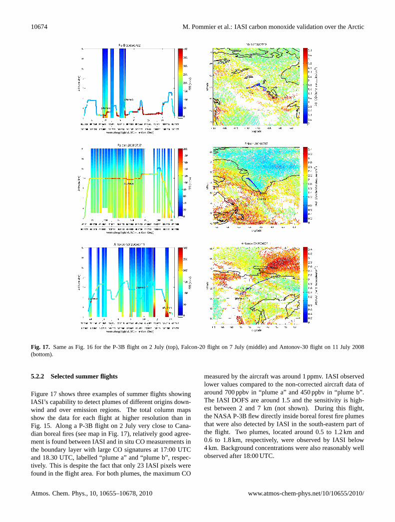
Fig. 9. Monthly averaged sea ice cover maps (white area) for April(a) and July 2008(b). The magenta line shows the 1979 to 2000 medianArctic sea-ice extent for each month (http://www.ncdc.noaa.gov/snow-and-ice/). The coloured crosses represent the positions of measuredCO profiles shown in Figs. 7 and 8.

Fig. 9a). This case shows a better sensitivity close to thesurface (and higher DOFS) compared to the two previousexamples over sea ice. Except on first level, the IASI andin situ smoothed profiles are quite similar (difference below20 ppbv). The last example (case (d)) was measured dur-ing the take-off of the ATR-42 in Sweden on 31 March (seeFig. 9a). IASI had problems detecting high CO signaturesmeasured by the aircraft between the surface to 6 km prob-ably due to the snow covering the land area (see data fromhttp://www.ncdc.noaa.gov/snow-and-ice/), and low thermalcontrast (see the AK plot) (|1T | ∼ 8.5 K). Another explana-tion could be the collocation. Only one IASI collocated pixelwas found and it was almost 50 min before the take-off so itis likely that IASI missed this plume. The difference betweenthe smoothed in situ and IASI values is around 50 to 60 ppbvin altitude range of the plume.

Overall in spring, retrievals over sea resolve better the ver-tical distribution than over sea ice or snow. The lack of ver-tical sensitivity and collocation issues were found to be themain reasons influencing plume detection in the IASI data.

4.4.2 Summer cases

A profile observed over Hudson Bay on 5 July shows thatthe DC-8 measured high CO concentrations between 5–8 km(see Fig. 8a). IASI was not able to locate precisely this signa-ture, but still captured an enhancement between 4 and 14 km.The smoothed in situ profile clearly illustrates the lack ofvertical resolution of the instrument resulting in a broad en-hancement in the mid-troposphere. IASI overestimates theCO concentration compared to the in situ smoothed profilewith a maximum mixing ratio at 10 km compared to 6 kmin the in situ profile. However, the ACE climatology is low


http://www.ncdc.noaa.gov/snow-and-ice/

http://www.ncdc.noaa.gov/snow-and-ice/


in this case. Tests using higher values for the climatologyin the UTLS (Upper Troposphere Lower Stratosphere) re-sults in the smoothed in situ profile becoming closer to theIASI profile suggesting that there could have been enhancedCO concentrations at this time. Also note that the presenceof sea ice in this area in spite of the season (see Fig. 9b)could explain the problem of retrieval with the limited verti-cal sensitivity. Moreover, the AK has higher values for thetwo first levels but many rows of the AK matrix are negativeat the surface making difficult the retrieval at these altitudes.This explains that the in situ smoothed profile is lower thanthe a priori below 3 km. Figure 8b shows a profile observedover a fire burning region in Siberia during the landing ofthe Antonov-30 in July 2008 (Fig. 9b). As in the case ofSiberian plume transport over Alaska in spring (Fig. 7b), theretrieval smoothes out enhanced CO at 1 km and 3 km dueto limited sensitivity for the levels below 3 km. This limitedsensitivity is probably due to low thermal contrast betweenthe surface and the first layers of atmosphere correspondingto the altitude of the biomass burning plume (|1T | ∼ 1.0 K).This result in differences ranging from 17 to 113 ppbv be-low 4.5 km between the IASI and smoothed in situ profiles.Above 7 km, (in the ACE-FTS climatology part) this differ-ence is around 10 ppbv. Case (c) was measured during anATR-42 take-off in Greenland on 10 July. Both IASI and theaircraft observed clean air with 8 IASI pixels found at almostthe same time as the take-off. The difference between thesmoothed in situ and IASI varies from 1 to 11 ppbv between8.5 km and 0.5 km, respectively. In this case, and consider-ing the size of the IASI footprint, it appears that the IASI datawas collected over snow-free land even though the Greenlandice sheet is situated about 100 km inland.

4.4.3 Summary

In summary, the lack of vertical sensitivity was found to bethe main detrimental factor for plume detection in the IASIdata. Surface type also has a major impact on the quality ofthe retrieval. Retrieval examples over snow in spring pro-vided similar results as over sea ice. Overall, IASI has bet-ter vertical resolution over land, particularly in summer, thanover the sea due to higher thermal contrast (Clerbaux et al.,2009). The vertical sensitivity is higher over land than oversnow or sea ice. In these examples, the DOFS varied withseason. It was around 1 in spring with a maximum of sensi-tivity between 2 and 10 km, and reached 1.7 in summer forthe Antonov-30 flight case with a peak of sensitivity at 1 to8 km, and a second peak at 10–13 km. The limited verticalsensitivity smoothed out most of pollution plumes but theapplication of the IASI AKs to the in situ measurements im-proves the agreement.

4.5 Results: statistical comparison of whole dataset

4.5.1 Comparison by aircraft

All IASI and smoothed in situ profiles were averaged by sea-son and by aircraft. We chose to compare the IASI retrievalsby aircraft because, as explained in Sect. 3, the aircraft didnot fly in the same regions or at the same time of year. There-fore, aircraft measured very different types of air mass rang-ing from flights over boreal fire regions and in air massesdownwind of anthropogenic emission regions. Figures 10and 11 show the comparison between IASI data and averagesof the aircraft observations from different spring and summercampaigns, respectively. The number of observations variesaccording to the aircraft from between 5 and 32 in springand 8 and 22 in summer. In spring, the mean smoothed in situprofiles are higher than mean IASI profiles above 6 km whichis generally where the climatology part applied. The differ-ence between both profiles reaches∼10 ppbv (17% maxi-mum) close to 10 km for the WP-3D and the ATR-42. Thisdifference is similar to the 15% bias found between ACE-FTS and MOZAIC in Clerbaux et al. (2008). For the DC-8, the smoothed in situ CO is always higher than IASI byonly a few ppbv (∼3–4 ppbv) and for the P-3B, both profilesare relatively similar up to 6 km. In summer, for each air-craft datasets, IASI CO is higher than smoothed in situ CObelow 8 km altitude where mainly in situ aircraft data wasused. This bias is found for all polluted cases. Moreover,with the DC-8 and P-3B is the smoothed in situ CO higherthan IASI CO at each level. The bias between the ATR-42and the Falcon-20, mentioned in Sect. 3.1, is not found inthis kind of comparison due to the smoothing with the IASIAK. The CO in situ profiles over Greenland from the ATR-42and the Falcon-20 are quite similar. Due to the lack of IASIvertical sensitivity at the lowest altitudes, maximum differ-ences are found at the surface (120 ppbv with the P-3B and20–30 ppbv with the other four aircraft). Nevertheless, therelative difference is always below 20% and in line to similarvalidation studies using MOPITT (Emmons et al., 2007) andTES (Lopez et al., 2008) at mid-latitudes. This seasonal dif-ference close to the surface is correlated to the IASI increasedsurface sensitivity in summer. The DOFS varies between 1.0and 1.10 in spring with a maximum of sensitivity between 2and 10 km, and in summer between 1.45 and 1.55 with gen-erally peak sensitivity at 2–8 km, and often a second regionof enhanced sensitivity at 9–12 km (not shown).

This comparison was also performed for total columnswith average values summarized in Table 3 for the springcampaigns, and Table 4 for the summer campaigns. Themean total columns from IASI and estimated from thesmoothed in situ profiles are in good agreement with an abso-lute value of relative differences ranging from 1.4% to 5.2%in spring with the WP-3D and the DC-8, respectively, andranging from 5 to 10% in summer. These results are con-sistent with previous validation studies (e.g. Emmons et al.,



31

Fig 10 Average IASI CO profiles (blue line) and smoothed in situ profiles (red line) in ppbv for 1207 each spring aircraft campaigns (left panel) and the relative difference (%) as given in Table 3 (thick 1208 blue line) and standard deviation (thin blue lines). The smoothed in situ profiles are the in situ 1209 aircraft measurements completed with the ACE-FTS climatology and convolved with IASI AK (see 1210 text for details). The horizontal black line represents the mean position of the maximum altitude 1211 reached by each particular aircraft. Errors bars represent the variability of measurements. 1212 1213 1214 1215 1216 1217

Fig. 10. Average IASI CO profiles (blue line) and smoothed in situ profiles (red line) in ppbv for each spring aircraft campaigns (left panel)and the relative difference (%) as given in Table 3 (thick blue line) and standard deviation (thin blue lines). The smoothed in situ profilesare the in situ aircraft measurements completed with the ACE-FTS climatology and convolved with IASI AK (see text for details). Thehorizontal black line represents the mean position of the maximum altitude reached by each particular aircraft. Errors bars represent thevariability of measurements.

Table 3. Average IASI and in situ smoothed CO total columns, standard deviations and relative differences calculated as followed: [((IASI-insitu)×2)/(IASI+in situ)]×100 for each spring campaign.

CO Total Column DC-8 P-3B ATR-42 WP-3D(1018 molecules/cm2)

IASI 2.22±0.32 2.16±0.38 2.45±0.28 2.25±0.30smoothed in situ∗ 2.19±0.33 2.15±0.17 2.56±0.19 2.37±0.14relative difference (%) 1.36 0.46 −4.39 −5.19

∗ See text for details.

Table 4. As Table 3 for each summer campaign.

CO Total Column DC-8 P-3B ATR-42 Falcon-20 Antonov-30(1018 molecules/cm2)

IASI 2.15±0.54 2.51±0.74 1.72±0.25 1.88±0.38 1.95±0.33smoothed in situ∗ 1.93±0.34 2.26±0.53 1.63±0.26 1.74±0.28 1.82±0.17relative difference (%) 10.78 10.48 5.37 7.73 6.90




32

Fig. 11 Same as Fig. 10 for summer campaigns. 1218 1219 Fig. 11. Same as Fig. 10 for summer campaigns.

2007) and show that for low DOFS, the differences for totalcolumns between IASI and the smoothed in situ measure-ments are low. For each summer case, the smoothed in situCO total column is lower than IASI CO total column; thisalso applies to two aircraft (DC-8 and P-3B) in spring. Fig-ure 12 shows the correlation between all CO total columndata. In both seasons the lowest correlation coefficient,r,is obtained in the comparison with the ATR-42 data withr = 0.15 in spring andr = 0.26 in summer. In spring, the cor-relation coefficient reaches 0.74 with the P-3B but it shouldbe noted that only 5 profiles were available. For the other

aircraft the correlation coefficient is 0.21 and 0.58 for DC-8and WP-3D, respectively. In summer, the highest correlation(r = 0.84) is found between IASI and the DLR Falcon datausing 16 profiles and ranges between 0.50 and 0.60 for theother aircraft.

Limiting the comparison to partial columns, comparingthereby the in situ part and not a combination of in situ andclimatology, improves the correlations in the 0 to 5 km layer,and varies between aircraft from 0.47 to 0.77 in spring andfrom 0.66 to 0.88 in summer (see Fig. 12). In both seasons,the correlations with the ATR-42, which flew to the lowest



33

Fig. 12 Scatter plots of IASI and smoothed in situ CO total columns (top) and 0-5 km partial 1239 columns (bottom) for the spring (left panel) and the summer (right panel) campaigns. The coloured 1240 lines represent the linear regression between data points for each aircraft: ATR-42 (magenta), DC-8 1241 (blue), P-3B (black), WP-3D (cyan), Falcon-20 (green), and Antonov-30 (red). The black dotted 1242 line, of unity slope, is shown for reference. 1243 1244 1245 1246 1247 1248 1249 1250 1251 1252 1253 1254 1255 1256

Fig. 12. Scatter plots of IASI and smoothed in situ CO total columns (top) and 0–5 km partial columns (bottom) for the spring (left panel)and the summer (right panel) campaigns. The coloured lines represent the linear regression between data points for each aircraft: ATR-42(magenta), DC-8 (blue), P-3B (black), WP-3D (cyan), Falcon-20 (green), and Antonov-30 (red). The black dotted line, of unity slope, isshown for reference.

maximum altitudes (up to 6–7 km), are the most improvedgiving 0.53 in spring and 0.70 in summer. In spring, the IASIcollocated profiles with the ATR-42 have the higher sensitiv-ity close to surface. These two factors highlight the impor-tance of a good climatology to complete the profile. Corre-lations between IASI and the combined dataset using all theaircraft data were also computed. In this case, differencesbetween aircraft measurements and sampling of different airmasses need to be kept in mind. The overall correlationsare 0.37 in spring and 0.67 in summer and improve to 0.59in spring and 0.79 in summer when only considering partialcolumns.

Moreover, these correlations also show, for total columnsas well as for partial columns, that when the correlation ishigher than 0.5, IASI values are generally lower than thesmoothed in situ values in spring and the inverse in summer.

Overall, this evaluation shows in the spring months maxi-mum differences above 6 km where the ACE climatology hasbeen used. This results in differences in the total columnsvarying between 1.4% and 5.20% (absolute values) accord-ing to aircraft. In summer IASI is always higher thansmoothed in situ vertical profiles (20%) leading to columndifferences of up to reaching 11% but correlations are betterdue to better IASI performance over the land. Again, for thelow flying aircraft results are improved when comparing justto partial columns.

4.5.2 Impact of surface type

Overall, the DOFS were around 1 in spring whatever surfacetypes and 1.6 over land, and 1.3 over the ocean in summer.This difference is related to a better thermal contrast in theradiance spectra measurements over land in summer wherethe diurnal surface temperature contrast is more intense thanover sea due to the limited heat water capacity (Clerbaux etal., 2009). In spring the maximum sensitivity is found be-tween 2 and 10 km for all surfaces. In summer there are twopeaks: between 1–8 km and 8–12 km over land, and between1–3 km and 4–11 km over the sea (not shown).

A study was performed to evaluate the impact of surfacetype on IASI CO measurements. All the profiles (and corre-sponding total columns) were averaged according to season,by aircraft, and then separated by sea and land surface type.It should be noted that during the spring campaigns, the samenumber of observations were performed over the land and sea(36 each) whereas in summer more profiles were obtainedover the land (68) with only 11 over the sea. Moreover, inspring most profiles were taken over snow or frozen sea.

In spring, over both surface types, the maximum differ-ence between smoothed in situ and the IASI profiles is closeto 10%. In spring, over land (Fig. 13a), IASI is similar orslightly higher than smoothed in situ measurements below6 km while over the sea (Fig. 13b) it is lower by a few ppbv.In summer, IASI is higher than the smoothed in situ below8.5 km over land and sea. Over land this difference variesfrom 0.2% (8.5 km) to 16% (0.5 km) (Fig. 13c) whereas over



34

Fig 13 Average IASI CO profiles (blue line) and smoothed in situ profiles (red line) in ppbv for 1257 each season (spring in top panels and summer in bottom panels), over land (figures a and c) and sea 1258 (b and d). Relative differences (see Table 5) (thick blue line) and standard deviation (thin blue lines) 1259 are also plotted as a function of altitude. The horizontal black line represents the mean position of 1260 the maximum altitude reached by each particular aircraft. Errors bars represent the variability of 1261 measurements. 1262 1263 1264 1265 1266 1267 1268 1269 1270 1271 1272 1273 1274 1275 1276 1277 1278 1279

Fig. 13. Average IASI CO profiles (blue line) and smoothed in situ profiles (red line) in ppbv for each season (spring in top panels andsummer in bottom panels), over land (a andc) and sea (b andd). Relative differences (see Table 5) (thick blue line) and standard deviation(thin blue lines) are also plotted as a function of altitude. The horizontal black line represents the mean position of the maximum altitudereached by each particular aircraft. Errors bars represent the variability of measurements.

the sea (Fig. 13d), IASI CO is about 10 ppbv (maximum11%) higher than smoothed in situ CO at all altitudes.

When comparing IASI CO total columns and the corre-sponding smoothed in situ data, a good correlation is foundover sea in spring (0.73) and over land in summer (0.69).Worse agreements are found in spring over the land (correla-tion 0.16) and over the sea in summer (0.33). Whatever thesurface type, in spring, the mean IASI total column is lowerthan the corresponding smoothed in situ total columns. Theopposite is found in summer (Table 5) with a maximum dif-ference of 12%. The comparison using just partial columns(0–5 km) again improves the correlations with 0.48 over theland and 0.78 over the sea for spring and with 0.81 over theland and 0.51 over the sea in summer (not shown).

Over both surface types, as the comparison by aircraft, westill observe a difference of 10% in spring between profiles.And IASI still has higher values than the smoothed in situvalues below 8.5 km in summer (maximum 16%) and for to-tal columns (maximum 12%).

5 Further insights into Arctic CO distributions

5.1 Spring and summer total columns

Figure 5 shows the average total CO columns for the monthof April and July in 2008. It highlights the seasonal cycleof CO with higher concentrations in spring due to its longerlifetime following accumulation during the winter, as well asthe main anthropogenic emission regions over Asia, NorthAmerica and Europe. Boreal fire regions can be seen inspring over Siberia and over Siberia and Canada in summer.Evidence for transport of enhanced CO downwind of conti-nental regions can also be seen.

During April 2008, pollution was transported from agri-cultural fires in eastern Europe/western Russia, boreal firesin Siberia and from anthropogenic source regions in Asiaacross the high Arctic Ocean. European pollution was alsotransported into northern Scandinavia. Plumes from Asia andEurope were observed by the ATR-42 (Adam de Villiers etal., 2010) and some across to Alaska and northern Canada(Warneke et al., 2009). Siberian burning plumes were trans-ported to Alaska by cyclonic activity near Lake Baikal andover the northern Pacific (Fuelberg et al., 2010). An exam-ple of the kind of measurements collected during spring is



Table 5. Average IASI and in situ smoothed CO total columns, standard deviations and relative differences calculated as followed: [((IASI-insitu)×2)/(IASI+insitu)]×100; for each season, according to surface type.

CO Total Column (1018 molecules/cm2) spring summer

land sea land sea

IASI 2.24±0.37 2.31±0.27 2.02±0.52 2.31±0.54smoothed in situ∗ 2.26±0.33 2.37±0.23 1.87±0.39 2.04±0.26relative difference (%) −0.89 −2.56 7.71 12.41


35

1280 a) b)

Fig. 14 ECMWF potential equivalent temperature at 850 hPa above Scandinavia (a) and daytime 1281 IASI CO total column map (b) on 31 March 2008. On both maps, the ATR-42 flight track is also 1282 shown (white line in panel (a) and blue line in panel (b)). 1283 1284 1285 1286 1287 1288 1289 1290 1291 1292 1293 1294 1295 1296 1297 1298 1299 1300 1301 1302 1303 1304 1305 1306 1307 1308 1309 1310 1311 1312 1313

Fig. 14. ECMWF potential equivalent temperature at 850 hPa above Scandinavia(a) and daytime IASI CO total column map(b) on 31March 2008. On both maps, the ATR-42 flight track is also shown (white line in panel a and blue line in panel b).

shown in Fig. 14 when, as part of POLARCAT-France, mea-surements were made north of Scandinavia. In this example,on 31 March 2008, IASI measurements show strong gradi-ents over this region (Fig. 14b). They correspond to the posi-tion of the polar front, which blocked European pollution tothe south (Fig. 14a). Note that since clouds were associatedwith the front and only clear-sky measurements are analysedwith IASI, there is a lack of IASI observations over this area.Moreover, the lower total column values over Spitsbergenshow the impact of topography and snow on the retrieval, orsea ice up to 82◦ N. This shows the impact of low sensitivityover sea ice or snow as observed with cases in Fig. 7.

Summer meteorological conditions were different and, ingeneral, weather systems were less intense during, for ex-ample, the ARCTAS-B period compared to the spring (Fu-elberg et al., 2010). During the aircraft campaigns basedin western Greenland in July 2008 rather clean air masseswere sampled at the beginning of the month. Then, a se-ries of low-pressure systems transported North American an-thropogenic pollution and Canadian biomass burning plumesover southern Greenland. This was followed by air massesarriving from the north transporting pollution from Siberianboreal fires or Asia anthropogenic emission regions. TheARCTAS-B flights sampled Canadian boreal fire plumes (Ja-cob et al., 2010) whereas the YAK flights sampled Siberian

fires (Paris et al., 2009). The daily coverage of IASI al-lows the detection of the CO long-range transport events. Anexample is illustrated in Fig. 15 which shows snapshots offour daily total column maps during July 2008. On 2 July2008 (Fig. 15a), CO source regions can be seen over Asiaand North America. CO plumes from Asia were transportedout of the continent and were divided into two branches on7 July (Fig. 15b), one part crossing the North Pole and thesecond reaching the western coast of North America. In ad-dition, North American plumes were transported across theNorth Atlantic towards Greenland by frontal systems. By the9 July (Fig. 15c), the Asian plume was transported directlyover the Arctic to Greenland and the North American plumeseither reached western Europe or were transported furthernorth over Greenland. The case of Asian plume transportover the Arctic to Greenland is discussed in detail in Soder-man et al. (2010). On 11 July (Fig. 15d), aged plumes canstill be seen over Greenland although they were diluted dueto mixing with cleaner air masses. Also due to higher orog-raphy over Greenland, CO enhancements (plumes) are lessevident in the IASI data.



36

1314 a) b)

c) d)

Fig. 15 Daily IASI CO total column maps on a 1°×1° grid for the 2 July (a), 7 July (b), 9 July (c) 1315 and 11 July (d) 2008. 1316 1317 1318 1319 1320 1321 1322 1323 1324 1325 1326

Fig. 15. Daily IASI CO total column maps on a 1◦× 1◦ grid for the 2 July(a), 7 July(b), 9 July(c) and 11 July(d) 2008.

5.2 Spatial plume distributions seen by IASI

In this section, we illustrate the ability of IASI to observeCO plumes at high spatial resolution given the spatial foot-print of the instrument. We also show direct comparisons be-tween the aircraft data and IASI data along the aircraft flighttracks, i.e. without accounting for the IASI limited verticalsensitivity. Since we show comparisons along horizontal andvertical legs of flights we have not applied the IASI AK inthese cases. This qualitative approach illustrates the abilityof IASI to detect different plumes at different altitudes andalso shows the influence of surface type on column retrievals.

5.2.1 Selected spring flights

Figure 16 shows three examples of CO distributions ob-served by the aircraft during spring flights of the DC-8,the ATR-42 and the WP-3D, along with the correspondingIASI retrievals highlighting the snow-sea ice/sea differencesdiscussed in Sect. 4.4.1. The number of IASI collocationwas 162, 29 and 44, respectively. On 9 April, the DC-8 flew across the North Pole from Iqaluit (eastern coast of

Canada) to Fairbanks (Alaska). IASI detected an enhance-ment due European pollution (seehttp://www.espo.nasa.gov/arctas/docs/flight/2008-4-9dc8 report.pdf) at the end of theflight (“plume a”) above the land between the ground and2 km. However, the retrieved concentrations are lower thanthe in situ measurement by about 40 ppbv. As discussed inSect. 4.4.1 and illustrated in Fig. 7a, the main part of theflight was above the sea ice or above the snow and most ofthe IASI CO data have a DOFS around 1.0 and thus a lack ofsensitivity at low altitudes.

On 10 April, IASI observed another plume (CO∼160 ppbv measured in situ) above the Arctic Ocean closeto the surface between 11:40 and 12:30 UTC. As shown inFig. 7c (corresponding to the second profile during this flight)the DOFS was around 1.10 in this region. Note that IASI didnot detect a CO signature in the first hour of this flight. Snowcovered land can explain this lack of vertical sensitivity. Thetotal IASI columns for this day clearly show plumes that havebeen transported from Asia which, as discussed in detail byAdam de Villiers et al. (2010), were mixtures of plumes orig-inating from Asian pollution and dust as well as Siberian for-est fire plumes. The comparison with the 31 March (Fig. 14)


http://www.espo.nasa.gov/arctas/docs/flight/2008-4-9_dc8_report.pdf

http://www.espo.nasa.gov/arctas/docs/flight/2008-4-9_dc8_report.pdf


37

Fig. 16 Left: Cross-sections, representing the CO mixing ratio measurements along the DC-8 flight 1327 on 9 April (top), the ATR-42 flight on 10 April (middle), and the WP-3D flight on 18 April 2008 1328 (bottom), compared with IASI CO distributions with a criteria of [±0.2°; ±1 h]. In situ CO is plotted 1329 by altitude versus UTC time along flight, represented by the curve, with latitude and longitude 1330 corresponding. Right: maps associated to the cross-sections show the flight track (blue) inside a full 1331 day of IASI CO total column observation (coloured dots). 1332

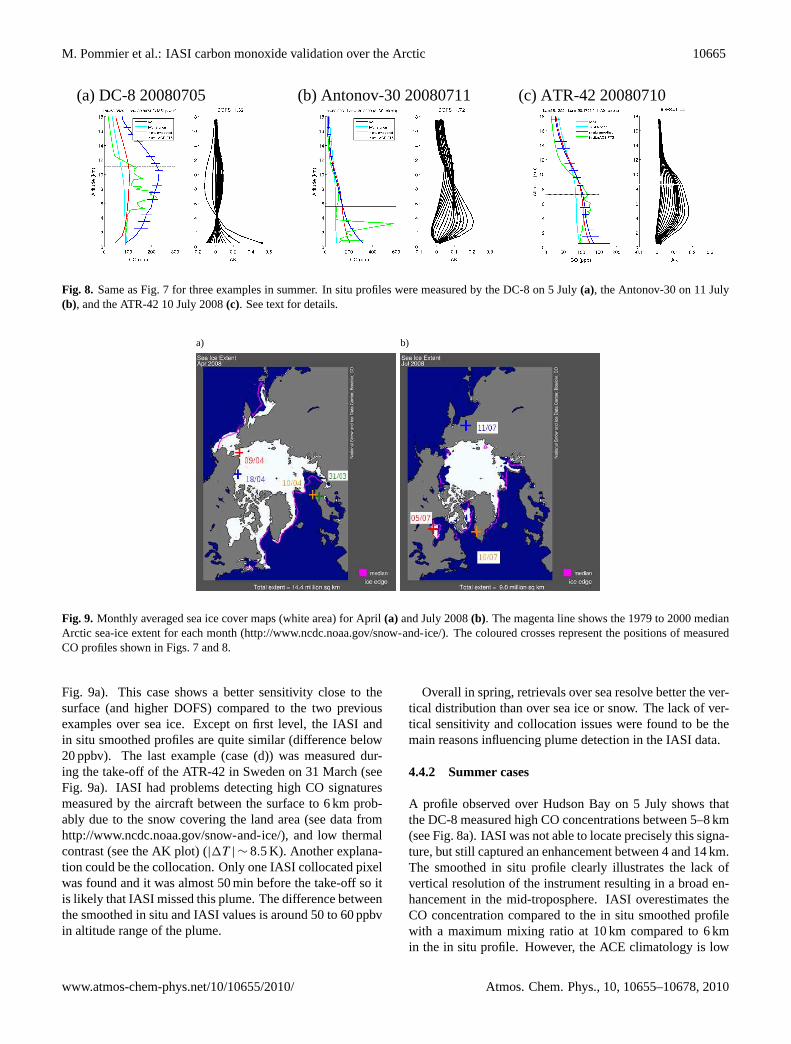
Fig. 16. Left: cross-sections representing the CO mixing ratio (in ppbv) measurements along the DC-8 flight on 9 April (top), the ATR-42flight on 10 April (middle), and the WP-3D flight on 18 April 2008 (bottom), compared with IASI CO distributions with a criterion of[±0.2◦; ±1 h]. In situ CO is plotted as a function of altitude versus UTC time along each flight. Corresponding aircraft positions in latitudeand longitude are also given. Right: day-time IASI CO column observations in molecules/cm2 in the region of the flights (track shown inblue).

shows the evolution of type of pollution, with an influenceof European pollution during first days of the POLARCAT-France campaign and Asian pollution at the end.

On 18 April, the WP-3D sampled a plume originatingfrom Kazakhstan agricultural fires (aged 7–9 days) anda forest fire plume from Lake Baikal, Siberia (aged 4–5 days). These plumes, identified in Fig. 16c as “plumea” and “plume b”, are described in detail by Warneke etal. (2009). IASI observed a signature of the agriculturalfire plumes around 4 km (“plume a”) corresponding to about

215 ppbv compared to 223 ppbv observed by the NOAA P3aircraft (maximum around 250 ppbv). IASI did not observeSiberian forest fire signature during the ascent and the de-scent around 23:00 UTC (plume b), due to the lack of sensi-tivity (DOFS∼1.0) over frozen sea at this time of year (seeFig. 7b). Nevertheless, enhanced CO was observed over thewhole region of the flight as shown in the total column map.



38

Fig. 17 Same as Fig. 16 for the P-3B flight on 2 July (top), Falcon-20 flight on 7 July (middle) and 1333 Antonov-30 flight on 11 July 2008 (bottom). 1334 1335 1336 1337

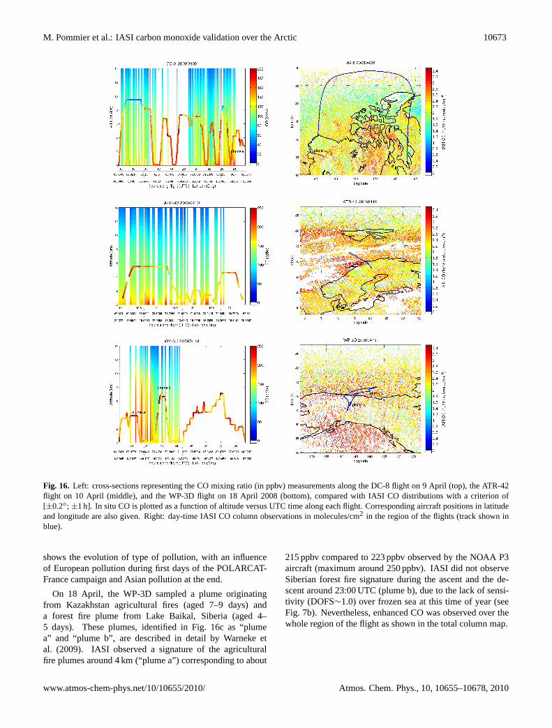
Fig. 17. Same as Fig. 16 for the P-3B flight on 2 July (top), Falcon-20 flight on 7 July (middle) and Antonov-30 flight on 11 July 2008(bottom).

5.2.2 Selected summer flights

Figure 17 shows three examples of summer flights showingIASI’s capability to detect plumes of different origins down-wind and over emission regions. The total column mapsshow the data for each flight at higher resolution than inFig. 15. Along a P-3B flight on 2 July very close to Cana-dian boreal fires (see map in Fig. 17), relatively good agree-ment is found between IASI and in situ CO measurements inthe boundary layer with large CO signatures at 17:00 UTCand 18.30 UTC, labelled “plume a” and “plume b”, respec-tively. This is despite the fact that only 23 IASI pixels werefound in the flight area. For both plumes, the maximum CO

measured by the aircraft was around 1 ppmv. IASI observedlower values compared to the non-corrected aircraft data ofaround 700 ppbv in “plume a” and 450 ppbv in “plume b”.The IASI DOFS are around 1.5 and the sensitivity is high-est between 2 and 7 km (not shown). During this flight,the NASA P-3B flew directly inside boreal forest fire plumesthat were also detected by IASI in the south-eastern part ofthe flight. Two plumes, located around 0.5 to 1.2 km and0.6 to 1.8 km, respectively, were observed by IASI below4 km. Background concentrations were also reasonably wellobserved after 18:00 UTC.



On 7 July, the Falcon-20 flew in a mixture of North Amer-ican forest fire and anthropogenic plumes in southern Green-land (see maps in Fig. 17 and Fig. 15b). A strong gradient isapparent between the plumes over the ocean and the ice sheetin Greenland still showing the problem of topography on to-tal columns values. Fifty-eight IASI collocations were foundwith a mean DOFS of 1.40 for this flight. The in situ mea-sured CO was around 160 ppbv and IASI CO observed about120 ppbv. The DLR Falcon-20 measured a more extensiveplume (in latitude) than IASI showing the IASI’s difficultiesto detect CO enhancement over the ice sheet.

On 11 July the Antonov-30 sampled forest fires plumesover Siberia during landing (“plume c”) (see also discussionin Sect. 4.4.2). This case is also described in detail in Paris etal. (2009). The plume was encountered at low altitudes in theboundary layer very close to the fire source region. IASI de-tected a signature around 350 ppbv when more than 600 ppbvwas measured by the aircraft. In this case, the IASI DOFSwas around 1.7 (see Fig. 8b). Two other CO plumes werealso observed by the aircraft during this flight (“plume a”and “plume b”) but were not detected by IASI. These plumeswere too thin for the satellite instrument vertical sensitivityto be detected. Concentrations in clean background air werealso well captured by IASI during the rest of the flight. Itmeans that, in this case, the a priori used in the retrieval isin good agreement with in situ observations. IASI also ob-served a CO plume transport further north and CO emissionsover western Siberia (not in the flight area). Overall, IASIachieves better vertical sensitivity in the summer over theArctic than in the spring, due to a higher thermal contrast,resulting in improved detection of CO plumes during thesehotter months.

6 Conclusions

This paper reports a detailed comparison of CO data obtainedfrom the IASI satellite-borne mission with in situ aircraftmeasurements measured as part of the POLARCAT projectin spring and summer 2008. Aircraft data were collected indifferent parts of the Arctic in air masses originating from an-thropogenic and forest fire emission regions. Data were alsocollected close to boreal forest fires over Siberia and Canada.IASI was able to detect several fire events as well as high COsignatures in the boundary layer due to forest fires in July2008. It also provides high spatial information about COplume distributions due to its high resolution footprint whichcan be used to interpret aircraft observations. We illustratedthat the detection of high CO events is more difficult oversea ice and snow because IASI CO retrievals show less sen-sitivity near the ground for cases associated with low thermalcontrast.

For the comparison IASI data were selected using a collo-cation criterion of [±0.2◦; ±1 h] around the flights. Relax-ing the collocation criterion did not lead to an improvement

in the results due to the fact that air masses of different ori-gin were likely to have been sampled. Aircraft profiles werecompleted with a seasonal and latitudinal climatology basedon ACE-FTS data averaged from 2004 to 2009 above aircraftmaximum flight ceilings and convolved with the IASI aver-aging kernels (called smoothed in situ profiles). Overall, theresults presented here show that IASI performs in Arctic aswell, or better than other satellite instruments measuring COwhich have been validated at mid-latitudes. In spring differ-ences of∼10 ppbv (maximum 17%) were found for the pro-files and between 1 to 5% for the total columns. In summer,for all the cases investigated, the difference between profilescan reach 20% below 8 km. For summertime total columnsa 12% maximum difference was found although this valuevaries as a function of surface type. Nevertheless, due toa better thermal contrast in summer and thus a better verti-cal sensitivity, more particularly over land, the correlationsfor total columns were better in summer from 0.26 to 0.84against from 0.15 to 0.74 in spring.

In spite of these difficulties, the analysis presented here hasshown the capability of IASI to observe long-range transportof CO into the Arctic and its potential to detect spatial andbroad vertical structure of pollutant plumes. This validationwork needs to be extended to other latitudes using other air-craft data (e.g. MOZAIC), and to other species (e.g. ozone)retrieved by IASI. Assimilation of IASI CO in global mod-els can be used to quantify pollution export to the Arctic, thebudgets of CO and ozone as well as to better constrain COsources.

Acknowledgements.M. Pommier was supported by a grant fromCNES (Centre national d’Etudes Spatiales) and by NOVELTIS.IASI was developed and built under the responsibility of CNESand flies onboard the MetOp satellite as part of the EumetsatPolar system. The IASI L1 data are received through the Eu-metcast near real time data distribution service. IASI L1 andL2 data are stored in the Ether French atmospheric database(http://ether.ipsl.jussieu.fr). We thank Raphael Adam de Villiersfor his contribution to this work. The research in Belgium wasfunded by the “Actions de Recherche Concertees” (CommunauteFrancaise), the Fonds National de la Recherche Scientifique(FRS-FNRS F.4511.08), the Belgian State Federal Office forScientific, Technical and Cultural Affairs and the European SpaceAgency (ESA-Prodex C90-327). POLARCAT-France was fundedby French ANR, CNES, CNRS-INSU (LEFE-CHAT), IPEVand also EUFAR. POLARCAT-GRACE was funded by DLR.The YAK-AEROSIB campaigns were funded by the CNRS-DRI(France), the French Ministry of Foreign Affairs, CEA (France),POLARCAT France/Norway, RAS (Russia) and RFBR (Russia),and operated in collaboration with IAO-SB-RAS, Tomsk, Russia.The ACE mission is supported primarily by the Canadian SpaceAgency and the UK Natural Environment Research Council(NERC). The authors are grateful to CNRS-INSU for publicationsupport.

Edited by: P. Monks


http://ether.ipsl.jussieu.fr


The publication of this article is financed by CNRS-INSU.

References

de Villiers, R. A., Ancellet, G., Pelon, J., Quennehen, B.,Schwarzenboeck, A., Gayet, J. F., and Law, K. S.: Airbornemeasurements of aerosol optical properties related to early springtransport of mid-latitude sources into the Arctic, Atmos. Chem.Phys., 10, 5011–5030, doi:10.5194/acp-10-5011-2010, 2010.

Ancellet, G., Leclair de Bellevue, J., Mari, C., Nedelec, P., Kukui,A., Borbon, A., and Perros, P.: Effects of regional-scale and con-vective transports on tropospheric ozone chemistry revealed byaircraft observations during the wet season of the AMMA cam-paign, Atmos. Chem. Phys., 9, 383–411, doi:10.5194/acp-9-383-2009, 2009.

Atlas, E. L., Ridley, B. A., and Cantrell, C. A.: The Tropo-spheric Ozone Production about the Spring Equinox (TOPSE)Experiment: Introduction, J. Geophys. Res., 108(D4), 8353,doi:10.1029/2002JD003172, 2003.

Badr, O. and Probert, S. D.: Carbon monoxide concentration in theEarth’s atmosphere, Appl. Energy, 50(4), 339–372, 1995.

Baehr, J., Schlager, H., Ziereis, H., Stock, P., van Velthoven, P.,Busen, R., Strom, J., and Schumann U.: Aircraft observationsof NO, NOy, CO, and O3 in the upper troposphere from 60◦ Nto 60◦S – Interhemispheric differences at midlatitudes, Geophys.Res. Lett., 30, 1598, doi:10.1029/2003GL016935, 2003.

Bernath, P. F., McElroy, C. T., Abrams, M. C., Boone, C. D., Butler,M., Camy-Peyret, C., Carleer, M., Clerbaux, C., Coheur, P.-F.,Colin, R., DeCola, P., DeMaziere, M., Drummond, J. R., Dufour,D., Evans, W. F. J., Fast, H., Fussen, D., Gilbert, K., Jennings, D.E., Llewellyn, E. J., Lowe, R. P., Mahieu, E., McConnell, J. C.,McHugh, M., McLeod, S. D., Michaud, R., Midwinter, C., Nas-sar, R., Nichitiu, F., Nowlan, C., Rinsland, C. P., Rochon, Y. J.,Rowlands, N., Semeniuk, K., Simon, P., Skelton, R., Sloan, J. J.,Soucy, M.-A., Strong, K., Tremblay, P., Turnbull, D., Walker, K.A., Walkty, I., Wardle, D. A., Wehrle, V., Zander, R., and Zou, J.:Atmospheric Chemistry Experiment (ACE): Mission overview,Geophys. Res. Lett., 32, L15S01, doi:10.1029/2005GL022386,2005.

Boone, C. D., Nassar, R., Walker, K.A., Rochon, Y., McLeod, S. D.,Rinsland, C. P., and Bernath, P. F.: Retrievals for the atmosphericchemistry experiment Fourier-transform spectrometer, Appl. Op-tics, 44, 7218–7231, 2005.

Boynard, A., Clerbaux, C., Coheur, P.-F., Hurtmans, D., Tur-quety, S., George, M., Hadji-Lazaro, J., Keim, C., and Meyer-Arnek, J.: Measurements of total and tropospheric ozone fromIASI: comparison with correlative satellite, ground-based andozonesonde observations, Atmos. Chem. Phys., 9, 6255–6271,doi:10.5194/acp-9-6255-2009, 2009.

Clarisse, L., Coheur, P. F., Prata, A. J., Hurtmans, D., Razavi,A., Phulpin, T., Hadji-Lazaro, J., and Clerbaux, C.: Trackingand quantifying volcanic SO2 with IASI, the September 2007

eruption at Jebel at Tair, Atmos. Chem. Phys., 8, 7723–7734,doi:10.5194/acp-8-7723-2008, 2008.

Clerbaux, C., Coheur, P.-F., Hurtmans, D., Barret, B., Carleer,M., Colin, R., Semeniuk, K., McConnell, J. C., Boone, C.,and Bernath, P.: Carbon monoxide distribution from the ACE-FTS solar occultation measurements, Geophys. Res. Lett., 32,L16S01, doi:10.1029/2005GL022394, 2005.

Clerbaux, C., George, M., Turquety, S., Walker, K. A., Barret, B.,Bernath, P., Boone, C., Borsdorff, T., Cammas, J. P., Catoire, V.,Coffey, M., Coheur, P.-F., Deeter, M., De Maziere, M., Drum-mond, J., Duchatelet, P., Dupuy, E., de Zafra, R., Eddounia,F., Edwards, D. P., Emmons, L., Funke, B., Gille, J., Griffith,D. W. T., Hannigan, J., Hase, F., Hopfner, M., Jones, N., Ka-gawa, A., Kasai, Y., Kramer, I., Le Flochmoen, E., Livesey,N. J., Lopez-Puertas, M., Luo, M., Mahieu, E., Murtagh, D.,Nedelec, P., Pazmino, A., Pumphrey, H., Ricaud, P., Rinsland, C.P., Robert, C., Schneider, M., Senten, C., Stiller, G., Strandberg,A., Strong, K., Sussmann, R., Thouret, V., Urban, J., and Wiacek,A.: CO measurements from the ACE-FTS satellite instrument:data analysis and validation using ground-based, airborne andspaceborne observations, Atmos. Chem. Phys., 8, 2569–2594,doi:10.5194/acp-8-2569-2008, 2008.

Clerbaux, C., Boynard, A., Clarisse, L., George, M., Hadji-Lazaro,J., Herbin, H., Hurtmans, D., Pommier, M., Razavi, A., Turquety,S., Wespes, C., and Coheur, P.-F.: Monitoring of atmosphericcomposition using the thermal infrared IASI/MetOp sounder, At-mos. Chem. Phys., 9, 6041–6054, doi:10.5194/acp-9-6041-2009,2009.

Coheur, P.-F., Herbin, H., Clerbaux, C., Hurtmans, D., Wespes, C.,Carleer, M., Turquety, S., Rinsland, C. P., Remedios, J., Hauglus-taine, D., Boone, C. D., and Bernath, P. F.: ACE-FTS observationof a young biomass burning plume: first reported measurementsof C2H4, C3H6O, H2CO and PAN by infrared occultation fromspace, Atmos. Chem. Phys., 7, 5437–5446, doi:10.5194/acp-7-5437-2007, 2007.

Coheur, P.-F., Clarisse, L., Turquety, S., Hurtmans, D., and Cler-baux, C.: IASI measurements of reactive trace species inbiomass burning plumes, Atmos. Chem. Phys., 9, 5655–5667,doi:10.5194/acp-9-5655-2009, 2009.

Emmons, L. K., Pfister, G. G., Edwards, D. P., Gille, J. C.,Sachse, G., Blake, D., Wofsy, S., Gerbig, C., Matross, D.,and Nedelec P.: Measurements of Pollution in the Troposphere(MOPITT) validation exercises during summer 2004 field cam-paigns over North America, J. Geophys. Res., 112, D12S02,doi:10.1029/2006JD007833, 2007.

Fehsenfeld, F. C., Ancellet, G., Bates, T. S., Goldstein, A. H., Hard-esty, R. M., Honrath, R., Law, K. S., Lewis, A. C., Leaitch, R.,McKeen, S., Meagher, J., Parrish, D. D., Pszenny, A. A. P., Rus-sell, P. B., Schlager, H., Seinfeld, J., Talbot, R., and Zbinden, R.:International Consortium for Atmospheric Research on Trans-port and Transformation (ICARTT): North America to Europe-Overview of the 2004 summer field study, J. Geophys. Res., 111,D23S01, doi:10.1029/2006JD007829, 2006.

Fisher, J. A., Jacob, D. J., Purdy, M. T., Kopacz, M., Le Sager,P., Carouge, C., Holmes, C. D., Yantosca, R. M., Batchelor,R. L., Strong, K., Diskin, G. S., Fuelberg, H. E., Holloway, J.S., Hyer, E. J., McMillan, W. W., Warner, J., Streets, D. G.,Zhang, Q., Wang, Y., and Wu, S.: Source attribution and in-terannual variability of Arctic pollution in spring constrained



by aircraft (ARCTAS, ARCPAC) and satellite (AIRS) observa-tions of carbon monoxide, Atmos. Chem. Phys., 10, 977–996,doi:10.5194/acp-10-977-2010, 2010.

Fuelberg, H. E., Harrigan, D. L., and Sessions, W.: A meteoro-logical overview of the ARCTAS 2008 mission, Atmos. Chem.Phys., 10, 817–842, doi:10.5194/acp-10-817-2010, 2010.

George, M., Clerbaux, C., Hurtmans, D., Turquety, S., Coheur, P.-F., Pommier, M., Hadji-Lazaro, J., Edwards, D. P., Worden, H.,Luo, M., Rinsland, C., and McMillan, W.: Carbon monoxide dis-tributions from the IASI/METOP mission: evaluation with otherspace-borne remote sensors, Atmos. Chem. Phys., 9, 8317–8330,doi:10.5194/acp-9-8317-2009, 2009.

Greenaway, K. R.: Experiences with Arctic flying weather, RoyalMeteorological Society Canadian Branch, 1950, Toronto, On-tario, Canada.

Harriss, R. C., Wofsy, S. C., Bartlett, D. S., Shipham, M. C., Jacob,D. J., Hoell Jr., J. M., Bendura, R. J., Drewry, J. W., McNeal, R.J., Navarro, R. L., Gidge, R. N., and Rabine, V. E.: The ArcticBoundary Layer Expedition (ABLE 3A): July–August 1988, J.Geophys. Res., 97(D15), 16383–16394, 1992.

Helmig, D., Oltmans, S. J., Morse, T. O., and Dibb, J. E.: What iscausing high ozone at Summit, Greenland?, Atmos. Environ., 41,5031–5043, 2007.

Herbin, H., Hurtmans, D., Clerbaux, C., Clarisse, L., and Coheur,P.-F.: H16

2 O and HDO measurements with IASI/MetOp, At-mos. Chem. Phys., 9, 9433–9447, doi:10.5194/acp-9-9433-2009,2009.

Holloway, J. S., Jakoubek, R., Parrish, D., Gerbig, C., Volz-Thomas, A., Schmitgen, S., Fried, A., Wert, B., Henry, B., andDrummond, J.: Airborne intercomparison of vacuum ultravioletfluorescence and tunable diode laser absorption measurements oftropospheric carbon monoxide, J. Geophys. Res.-Atmos., 105,24251–24261, 2000.

Jacob, D. J., Crawford, J. H., Maring, H., Clarke, A. D., Dibb, J. E.,Emmons, L. K., Ferrare, R. A., Hostetler, C. A., Russell, P. B.,Singh, H. B., Thompson, A. M., Shaw, G. E., McCauley, E., Ped-erson, J. R., and Fisher, J. A.: The Arctic Research of the Com-position of the Troposphere from Aircraft and Satellites (ARC-TAS) mission: design, execution, and first results, Atmos. Chem.Phys., 10, 5191–5212, doi:10.5194/acp-10-5191-2010, 2010.

Law, K. S. and Stohl, A.: Arctic Air Pollution: Origins and Impacts,Science, 315, 1537–1540, doi:10.1126/science.1137695, 2007.

Lopez, J. P., Luo, M., Christensen, L. E., Loewenstein, M., Jost, H.,Webster, C. R., and Osterman, G.: TES carbon monoxide valida-tion during two AVE campaigns using the Argus and ALIAS in-struments on NASA’s WB-57F, J. Geophys. Res., 113, D16S47,doi:10.1029/2007JD008811, 2008.

McMillan, W. W., Warner, J. X., McCourt Comer, M., Maddy,E., Chu, A., Sparling, L., Eloranta, E., Hoff, R., Sachse, G.,Barnet, C., Razenkov, I., and Wolf, W.: AIRS views trans-port from 12 to 22 July 2004 Alaskan/Canadian fires: Corre-lation of AIRS CO and MODIS AOD with forward trajecto-ries and comparison of AIRS CO retrievals with DC-8 in situmeasurements during INTEX-A/ICARTT, J. Geophys. Res., 113,D20301, doi:10.1029/2007JD009711, 2008.

Mitchell Jr., J. M.: Visual range in the polar regions with particularreference to the Alaskan Arctic, J. Atmos. Terr. Phys., SpecialSuppl., Pt. I, 195–211, 1957.

Nedelec, P., Cammas, J.-P., Thouret, V., Athier, G., Cousin, J.-M.,

Legrand, C., Abonnel, C., Lecoeur, F., Cayez, G., and Marizy,C.: An improved infrared carbon monoxide analyser for routinemeasurements aboard commercial Airbus aircraft: technical val-idation and first scientific results of the MOZAIC III programme,Atmos. Chem. Phys., 3, 1551–1564, doi:10.5194/acp-3-1551-2003, 2003.

Paris, J.-D., Ciais, P., Nedelec, P., Ramonet, M., Belan, B. D., Ar-shinov, M. Y., Golitsyn, G. S., Granberg, I., Stohl, A., Cayez, G.,Athier, G., Boumard, F., and Cousin, J. M.: The YAK-AEROSIBtranscontinental aircraft campaigns: new insights on the trans-port of CO2, CO and O3 across Siberia, Tellus B, 60 (4), 551–568, 2008.

Paris, J.-D., Stohl, A., Nedelec, P., Arshinov, M. Yu., Panchenko,M. V., Shmargunov, V. P., Law, K. S., Belan, B. D., and Ciais, P.:Wildfire smoke in the Siberian Arctic in summer: source charac-terization and plume evolution from airborne measurements, At-mos. Chem. Phys., 9, 9315–9327, doi:10.5194/acp-9-9315-2009,2009.

Provencal, R., Gupta, M., Owano, T.G., Baer, D. S., Ricci, K. N.,O’Keefe, A., and Podolske, J. R.: Cavity-enhanced quantum-cascade laser-based instrument for carbon monoxide measure-ments, Appl. Optics, 44(31), 6712–6717, 2005.

Razavi, A., Clerbaux, C., Wespes, C., Clarisse, L., Hurtmans, D.,Payan, S., Camy-Peyret, C., and Coheur, P. F.: Characterizationof methane retrievals from the IASI space-borne sounder, At-mos. Chem. Phys., 9, 7889–7899, doi:10.5194/acp-9-7889-2009,2009.

Rinsland, C. P., Dufour, G., Boone, C. D., Bernath, P. F., Chiou,L., Coheur, P.-F., Turquety, S., and Clerbaux, C.: Satellite bo-real measurements over Alaska and Canada during June–July2004: Simultaneous measurements of upper tropospheric CO,C2H6, HCN, CH3Cl, CH4, C2H2, CH3OH, HCOOH, OCS,and SF6 mixing ratios, Global Biogeochem. Cy., 21, GB3008,doi:10.1029/2006GB002795, 2007.

Rodgers, C. D.: Inverse methods for atmospheric sounding: the-ory and practice, Ser. Atmos. Ocean. Planet. Phys. 2, World Sci.,Hackensack, NJ, 2000.

Rodgers, C. D. and Connor, B. J.: Intercomparison of re-mote sounding instruments, J. Geophys. Res., 108(D3), 4116,doi:10.1029/2002JD002299, 2003.

Sachse, G. W. ,Hill, G. F., Wade, L. O., and Perry, M. G.: Fastresponse, high precision carbon monoxide sensor using a tunablediode laser absorption technique, J. Geophys. Res., 92, 2071–2081, 1987.

Schlussel, P., Hultberg, T. H., Phillips, P. L., August, T., and Calbet,X.: The operational IASI Level 2 processor, Adv. Space Res., 36,982–988, 2005.

Shindell, D., Faluvegi, G., Lacis, A., Hansen, J., Ruedy, R.,and Aguilar, E.: Role of tropospheric ozone increases in20th-century climate change, J. Geophys. Res., 111, D08302,doi:10.1029/2005JD006348, 2006.

Shindell, D. T., Chin, M., Dentener, F., Doherty, R. M., Faluvegi,G., Fiore, A. M., Hess, P., Koch, D. M., MacKenzie, I. A.,Sanderson, M. G., Schultz, M. G., Schulz, M., Stevenson, D.S., Teich, H., Textor, C., Wild, O., Bergmann, D. J., Bey, I.,Bian, H., Cuvelier, C., Duncan, B. N., Folberth, G., Horowitz, L.W., Jonson, J., Kaminski, J. W., Marmer, E., Park, R., Pringle,K. J., Schroeder, S., Szopa, S., Takemura, T., Zeng, G., Keat-ing, T. J., and Zuber, A.: A multi-model assessment of pollu-



tion transport to the Arctic, Atmos. Chem. Phys., 8, 5353–5372,doi:10.5194/acp-8-5353-2008, 2008.

Sodemann, H., Pommier, M., Arnold, S. R., Monks, S. A., Stebel,K., Burkhart, J. F., Hair, J. W., Diskin, G. S., Clerbaux, C., Co-heur, P.-F., Hurtmans, D., Schlager, H., Blechschmidt, A.-M.,Kristjansson, J. E., and Stohl, A.: Episodes of cross-polar trans-port in the Arctic troposphere during July 2008 as seen frommodels, satellite, and aircraft observations, Atmos. Chem. Phys.Discuss., 10, 26361–26410, doi:10.5194/acpd-10-26361-2010,2010.

Stohl, A.: Characteristics of atmospheric transport intothe Arctic troposphere, J. Geophys. Res., 111, D11306,doi:10.1029/2005JD006888, 2006.

Turquety, S., Logan, J. A., Jacob, D. J., Hudman, R. C., Leung,F. Y., Heald, C. L., Yantosca, R. M., Wu, S., Emmons, L. K.,Edwards, D. P., and Sachse, G. W.: Inventory of boreal fire emis-sions for North America in 2004: the importance of peat burningand pyro-convective injection, J. Geophys. Res., 112, D12S03,doi:10.1029/2006JD007281, 2007.

Turquety, S., Clerbaux, C., Law, K., Coheur, P.-F., Cozic, A., Szopa,S., Hauglustaine, D. A., Hadji-Lazaro, J., Gloudemans, A. M.S., Schrijver, H., Boone, C. D., Bernath, P. F., and Edwards,D. P.: CO emission and export from Asia: an analysis com-bining complementary satellite measurements (MOPITT, SCIA-MACHY and ACE-FTS) with global modeling, Atmos. Chem.Phys., 8, 5187–5204, doi:10.5194/acp-8-5187-2008, 2008.

Turquety, S., Hurtmans, D., Hadji-Lazaro, J., Coheur, P.-F., Cler-baux, C., Josset, D., and Tsamalis, C.: Tracking the emissionand transport of pollution from wildfires using the IASI CO re-trievals: analysis of the summer 2007 Greek fires, Atmos. Chem.Phys., 9, 4897–4913, doi:10.5194/acp-9-4897-2009, 2009.

Wan, Z.: New refinements and validation of the MODIS land-surface temperature/emissivity products, Remote Sens. Environ.,112, 59–74, 2008.

Warneke, C., Bahreini, R., Brioude, J., Brock, C. A. , de Gouw, J.A. , Fahey, D. W. , Froyd, K. D. , Holloway, J. S., Middlebrook,A., Miller, L. , Montzka, S., Murphy, D. M., Peischl, J., Ryerson,T. B., Schwarz, J. P., Spackman, J. R., and Veres, P.: Biomassburning in Siberia and Kazakhstan as an important source forhaze over the Alaskan Arctic in April 2008, Geophys. Res. Lett.,36, L02813, doi:10.1029/2008GL036194, 2009.

Wespes, C., Hurtmans, D., Clerbaux, C., Santee, M. L., Martin,R. V., and Coheur, P. F.: Global distributions of nitric acid fromIASI/MetOP measurements, Atmos. Chem. Phys., 9, 7949–7962,doi:10.5194/acp-9-7949-2009, 2009.

Yurganov, L. N., McMillan, W. W., Dzhola, A. V., Grechko, E. I.,Jones, N. B., and van der Werf, G. R.: Global AIRS and MO-PITT CO measurements: Validation, comparison, and links tobiomass burning variations and carbon cycle, J. Geophys. Res.,113, D09301, doi:10.1029/2007JD009229, 2008.


Documents

IASI carbon monoxide validation over the Arctic during ... · M. Pommier et al.: IASI carbon monoxide validation over the Arctic 10657 Sect. 3. Section 4 describes the collocation