Embed Size (px)
Citation preview

I WANT TO RIDE MY BICYCLE: THE RELATIONSHIP BETWEEN BICYCLE
INFRASTRUCTURE AND COMMUTING BY CAR IN U.S. CITIES
A Thesis submitted to the Faculty of the
Graduate School of Arts and Sciences of Georgetown University
in partial fulfillment of the requirements for the degree of
Master of Public Policy in Public Policy
By
Rebecca Stewart, B.A.
Washington, DC April 17, 2013

ii
Copyright 2013 by Rebecca Stewart All Rights Reserved
iii
I WANT TO RIDE MY BICYCLE: THE RELATIONSHIP BETWEEN BICYCLE INFRASTRUCTURE AND COMMUTING BY CAR IN U.S. CITIES
Rebecca Stewart, B.A
Thesis Advisor: Adam T. Thomas, Ph.D.
ABSTRACT
In American cities over the last several years, bicycle ridership and related infrastructure have
surged upward as traffic congestion has steadily worsened. Policymakers see additional bicycle-
specific infrastructure as a way to decrease the adverse effects of congestion on the road and
promote the health and economic benefits that result from bicycle riding. While much
scholarship studies the impact of bicycle lanes and trails on bicycle ridership, little research
assesses the relationship between the existence of bicycle lanes and trails and rates of commuting
by car. Using city-year panel data from 2007, 2009, and 2011, this analysis examines the
possible association between bicycle infrastructure per square mile and rates of commuting by
car in 51 U.S. cities. While fixed effects models do not provide evidence of a statistically
significant relationship between bicycle infrastructure and commuting by car, regular multiple
regression suggests a weak negative relationship between these two variables.

iv
TABLE OF CONTENTS
Introduction ..................................................................................................................... 1 Background ...................................................................................................................... 2 Literature Review ............................................................................................................ 6 Conceptual Framework and Hypothesis ........................................................................ 10 Data and Methods .......................................................................................................... 12 Descriptive Statistics ..................................................................................................... 16 Regression Results ......................................................................................................... 20 Discussion ...................................................................................................................... 24 References ..................................................................................................................... 28

v
LIST OF FIGURES AND TABLES
Figure 1: Factors Affecting the Decision to Commute by Car ...................................... 11 Table 1: Variable Definitions ........................................................................................ 15 Table 2: City and Individual Level Characteristics ....................................................... 18 Table 3: Correlation Matrix: Percentage Commuting by Car and Bicycle Infrastructure Per Square Mile ............................................................................................................ 19 Table 4: OLS and Fixed Effect Regression Results ...................................................... 21 Table 5: Joint Significance Test Results ....................................................................... 23
1
INTRODUCTION
Traffic congestion in American cities has worsened steadily over the last several years.
(Hartgen & Fields, 2006). Commuting alone by car remains the norm; in 2011, 86.6% of
commuters drove to work and 88.8% of them (about 76% of total commutes) did so alone (U.S.
Census Bureau, 2011). Annual rush hour delays for the average driver in urban areas with
populations above one million rose by 30 hours from 1982 to 2010, more than tripling from 14 to
44. Outside of rush hour, congestion has also gotten worse, with 40% of delays occurring at non-
rush hour times. The estimated cost of congestion based on wasted time and fuel is over $100
billion, or nearly $750 for every commuter in the U.S. (Shrank, Lomax, & Eisele, 2011). At the
same time that congestion has worsened, cities have grown. In 2011, urban population growth
outpaced that of the suburbs for first time in decades (Frey, 2012).
As a result of the challenges of city driving, commuting by bicycle has come into vogue
in urban areas. Cycling is associated with many positive returns, including reductions in obesity,
harmful emissions, traffic, and necessary road infrastructure; better health and economic
outcomes; increased physical activity; and aggregate- and individual-level savings on car and
public transportation costs (Ming Wen & Rissel, 2008; Frank, Andresen, & Schmid, 2004;
Cooper, Andersen, Wedderkopp, Page, & Froberg, 2005; Garrett-Peltier, 2010; Horner, 2012;
Gotschi & Mills, 2008). de Hartog, Boogaard, Nijland, and Hoek (2010) found that the benefits
attributable to shifting from commuting by car to commuting by bicycle (adding 3-14 months to
one’s life) outweighed the risks, given the relatively small reductions in life expectancy
associated with increased inhalation of air pollution (.8 to 40 days) and the higher probability of
being in a traffic accident (5 to 9 days).
2
As cycling has become increasingly popular, there has been a corresponding growth in
bicycle-specific infrastructure, including on-street bike lanes, multiuse and bike paths, and
signed bike routes. In some places, bicycle infrastructure miles have more than tripled since
2007, rising from 120 to 374 in Fresno and from 295 to 686 in Albuquerque (Alliance for Biking
and Walking, 2012). People tend to feel safer when using dedicated bike facilities, making
bicycling a more attractive option (U.S. Department of Transportation, 2010). As such,
concurrent with the increase in bicycle facilities, the number of people who bicycle to work
soared 67% between 2000 and 2011, from 466,856 to 777,585 (U.S. Census Bureau, 2000; U.S.
Census Bureau, 2011).
These dynamics beg the question: has the increase in bicycle infrastructure in cities
affected rates of commuting by car? Logically, it would follow that if more people are cycling,
fewer must be driving, resulting in less congestion and a diminution of the other harmful effects
of car use. Nonetheless, it is possible that those who choose to commute by bicycle would
otherwise commute on foot or by public transportation, rather than by car. In examining whether
bicycle lanes are a viable option to reduce congestion, decrease harmful emissions, and promote
health in cities, I find that there is a very small but statistically significant association between
increased bicycle infrastructure and decreased commuting by car. Future researchers should
collect more and standardized data as well as include additional variables to control for further
omitted variable bias in order to gain a fuller picture of this relationship.
BACKGROUND
Federal legislation influences how states and local entities spend transportation funds,
shaping policies at all levels of government by stipulating the use of monies for particular
3
programs. Given the increases in both congestion and bicycle ridership, the relationship between
commuting by car and bicycle infrastructure has important implications for the way in which
funds should be distributed in the future in order to maximize the positive impact on American
cities.
The $286 billion Safe, Accountable, Flexible, and Efficient Transportation Equity Act: A
Legacy for Users (2005) (SAFETEA-LU) was enacted in August 2005 and expired on
September 30, 2009. This legislation laid the basic federal framework for smart transportation
planning, bicycle and pedestrian infrastructure, highway maintenance and improvement, and
congestion mitigation. Additionally, the 2009 American Recovery and Reinvestment Act
invested substantially in bicycle and pedestrian projects, with $750 million allocated for that
purpose in a one-time infusion. Those funds have since been expended. Congress renewed the
SAFETEA-LU funding formula several times until the law was finally replaced by the two-year
$105 billion Moving Ahead for Progress in the 21st Century Act (MAP-21) in July 2012 (De
Zeeuw & Flusch, 2011).
In 2011, less than 2% of SAFETEA-LU’s $40 billion in federal transportation funding
went to pedestrian and bicycle programs, distributed across three major programs (De Zeeuw &
Flusch, 2011). First, the Surface Transportation Program, a flexible program used largely for
highway improvements, sets aside 10% for Transportation Enhancements specifically for cycling
and walking projects, including bicycling and walking facilities, historic preservation,
environmental mitigation, and “rails to trails” conversion of railway corridors to pedestrian and
bicycle trails. Second, the Safe Routes to Schools program funds the construction of safe
pedestrian and cycling routes within two miles of schools (De Zeeuw & Flusch, 2011). These
routes are intended to encourage children to walk or bike to school since only 12.7 % of K-8

4
children did so in 2009, down from 47.7% of children in 1969 (McDonald, Brown, Marchetti, &
Pedroso, 2011). Finally, the Recreational Trails Program funds recreational trail creation,
maintenance, and support (De Zeeuw & Flusch, 2011).
SAFETEA-LU (2005) also contained a variety of provisions specifically related to
automobile congestion. These include the Real-Time System Management Program, which
allows officials to monitor road conditions instantly and share information with the public to
alleviate congestion and facilitate travel decision making; road pricing programs; high
occupancy vehicle lanes; and the Congestion Mitigation and Air Quality Improvement (CMAQ)
program, which provides flexible funding for states and local governments to spend on
transportation projects in order to meet Clean Air Act requirements. Additionally, other portions
of the legislation provided flexible funding that could be used for congestion reduction purposes.
SAFETEA-LU ‘s replacement, MAP-21 (2012), does not fundamentally alter the existing
transportation framework. However, it does reduce significantly the amount of funds that must
be spent specifically on bicycle and pedestrian facilities, with a possible drop of 33-66%,
depending on how states choose to allocate these dollars (Hall, 2012). In terms of congestion
control and in contrast to SAFETEA-LU, MAP-21 provides funding for transportation projects
that reduce congestion generally but leaves it up to the states to decide whether these funds are
best spent on projects such as highway improvement programs, recreational trails, safe routes to
school, bicycling programs, or road improvements. In the absence of strong federal guidance, the
removal of spending requirements may lead state and local governments to divert those monies
away from bicycle infrastructure.
MAP-21 also combined the bicycling and pedestrian programs Recreational Trails,
Transportation Enhancements, and Safe Routes to Schools into the new Transportation
5
Alternatives program, to be distributed via a competitive process (Hall, 2012). In combination
with the overall decrease in available funds, the threat of fund redistribution away from bicycling
and walking programs, and the introduction of new entities eligible to receive funds, this policy
change may stymie bicycle infrastructure projects. It is important to note that lawmakers have
disproportionately targeted bicycle and pedestrian funds for rescission. For instance, in 2010,
Transportation Enhancements and CMAQ funding made up 7.3% of state Departments of
Transportation funding but comprised 44% of funds rescinded that year (Alliance for Bicycling
and Walking, 2012). In fact, 21% of total Transportation Enhancements funding has been
rescinded since 1992 (Alliance for Bicycling and Walking, 2012).
States and localities enact a variety of policies to make cycling a more attractive option
for commuters, including public information activities; publicly available bicycle maps; bicycle
master plans; “complete streets” policies, where all users of streets must be accommodated;
advisory committees; bicycle-friendly legislation, including passing distance laws; bicycle
parking spaces; “share the road” campaigns; and statewide rides; among others. Even so, states
spent only 1.6% of federal transportation dollars on bicycling and walking from 2006-2010, or
just $2.17 per capita (Alliance for Bicycling and Walking, 2012).
Clearly, federal, state, and local policy play a large role in determining the trajectory of
transportation planning. For cities that wish to reduce their congestion due to excessive
automobile traffic, it seems logical to assume that investing in bicycle infrastructure would cause
people who ordinarily drive to work to take advantage of the opportunity to commute by bicycle.
But it is also possible that those who use bicycle infrastructure are substituting for walking to
work or taking public transportation, in which case there would be no correlation. Currently,

6
there is no demonstrated link between bicycle infrastructure and commuting by car; this paper
explores that relationship.
LITERATURE REVIEW
Understanding why people choose to commute by car is integral to the study of any
policy intended to mitigate congestion. Commuting to work by car is the default in the United
States; the National Household Transportation Survey (NHTS) reports that, from 1969-2009, the
percentage of people commuting to work in privately-owned vehicles remained steady at around
90%, with 151 million people commuting to work by privately-owned vehicle in 2009. Car
commuters rarely cycle to work; only 1% of commuters who usually drove alone commuted by
bicycle on the day recorded. (U.S. Department of Transportation, 2009).
Much of the extant research on bicycle infrastructure and commuting focuses on the
former’s effect on commuting by bicycle rather than on other modes. Research suggests that
cycling levels and the miles of available bicycle paths and lanes are positively correlated. Using
data from 90 of the 100 largest U.S. cities, Buehler and Pucher (2012) found that cities with
more bicycle paths had significantly higher bicycle commuting rates. Nelson and Allen (1997),
using a cross-sectional dataset of 18 U.S. cities, found that the addition of one mile of bicycle
paths or lanes per 100,000 residents was associated with a .069% increase in the number of
commuters who cycle to work. A cross-sectional analysis of data from 35 cities across the U.S.
expanded upon Nelson and Allen’s work, finding that adding a mile of bicycle lanes per square
mile in cities was correlated with an increase of approximately 1% in the bicycle commuting rate
(Dill & Carr, 2003).

7
Evidence suggests that increasing funding for bicycle infrastructure is associated with an
increase in the number of cyclists on the roads (Garrard, Rose, & Lo, 2008; Pucher & Buehler,
2007; Pucher & Buehler, 2008). Gotschi and Mills’s (2008) cross-country study found a positive
relationship between metropolitan investment in bicycling and the level of bicycle travel.
Researchers have also found that car commuting choice is associated with a number of
individual-level characteristics. In 2011, researchers analyzing the NHTS found an inverse
relationship between car ownership and levels of walking and bicycling (Pucher, Buehler,
Merom, & Bauman, 2011). Dargay and Hanly (2007) found that working part time and living in
a single-person household were negatively related to commuting by car, and that households
containing more than one adult and/or self-employed individuals were more likely to commute
by car. Women make up 44% of car commuters while men make up 56% (U.S. Department of
Transportation, 2009). Environmentally conscious households tend to drive 450 fewer miles per
year than less “green” ideologically inclined households (Kahn & Morris, 2009). In addition,
living in an urban or diverse land use area is negatively correlated with commuting by car
(Winters, Friesen, Koehoorn, & Teschke, 2007).
Cyclist commuters also tend to share some common demographic features. Male cyclists
far outnumber female cyclists, with 76% of trips made by men. Researchers found that, in cities,
men accounted for all of the growth in cycling from 2001 to 2009 (Pucher, Buehler, & Seinen,
2011). Women tend to prefer off-road paths over on-road lanes or roads with no bike facilities
(Garrard et al., 2008). Plaut (2005) found that those who choose to bike or walk to work tend to
be younger and better educated. Kahn and Morris (2009) found that living in a “green” voting
district is associated with choosing more environmentally friendly commuting options, including
the use of a bicycle to get to work.
8
The literature is unclear as to the relationship between income and commuting choices.
Plaut (2005) found income and car commuting to be positively associated. However, Krizek,
Barnes, and Thompson (2009), using census data from 1990 and 2000 in the Minneapolis-St.
Paul area, found income to be positively correlated with bicycle commuting for those with
annual incomes below $15,000 or over $50,000. Dill and Carr (2003), meanwhile, found no
association between income and cycling rates.
Geographic considerations also seem to have an influence on commuting choices, but
once again, some research findings are contradictory. Bergstrom and Magnussen (2003) found
that, in winter, there is a 47% decrease in bicycle trips and 27% increase in car trips, and Winters
et al. (2007) found the number of days with freezing temperatures to be negatively related to
cycling.1 In contrast, Yang, Roux, and Bingham (2011) found that people walk and cycle to
work, school, and other destinations less in the southern United States in general, which has a
warmer climate than the rest of the country.
Safety on the roads is another important determinant of commute mode choice. Dill and
Voros (2007) found that the majority of respondents to a phone survey on bicycling attitudes
wanted to cycle more and cited the lack of bike lanes or trails as the second biggest reason for
why they did not. Jacobsen (2003) found an inverse relationship between levels of cycling and
walking and the likelihood of being struck by a motorist. This suggests that the more cyclists and
walkers there are on the road, the more likely it is that motorists will be alert to the associated
dangers and risks and modify their behavior accordingly. A review of existing bicycle
infrastructure research found that bicycle-specific infrastructure is associated with the lowest risk
of bicycle injuries and crashes; that sidewalks and multi-use trails are associated with the highest
risk; and that major roads are more hazardous than minor roads (Reynolds, Harris, Teschke, 1 While the Bergstrom and Magnussen survey was conducted in Sweden, which has harsher winters than most of the

9
Cripton, & Winters, 2009). The National Bicycling and Walking Study found that dedicated
cycling lanes help to foster a feeling of safety among cyclists and may be necessary in order to
realize substantial increases in bicycle ridership (U.S. Department of Transportation, 2010).
More specifically, researchers found a strong correlation between bikeway network size and
bicycle commuting. Dill and Voros (2007) found that people listed “too much traffic” as the
biggest reason why they did not cycle more often, and Tilahun, Levinson, and Krizek (2007)
found that individuals would cycle up to 23 minutes out of their way to use an off-road bike lane
rather than a road with traffic and side parking.
Commute length may play a role in commuting choices as well. Over the last several
decades, commutes have lengthened in both distance and time (U.S. Department of
Transportation, 2009). Plaut (2005) found that people are more likely to commute by car when
their commutes are longer. Similarly, Cervero and Duncan (2003) found that people with shorter
commutes are more likely to cycle to work.
The literature suggests that other assorted factors may be important for this analysis.
Specifically, gasoline prices are negatively related to the number of trips by car and positively
related to the number of trips by public transportation, foot, and bike (Buehler, 2010).
Additionally, Limtanakool, Dijst, and Schwanen, (2006) found that the availability of public
transportation options is negatively related to car commuting. Areas with shorter travel times due
to compact infrastructure tend to have higher commuter cycling rates (Zahran, Brody, Maghelal,
Prelog, & Lacy, 2008). Diversity in the land use due to mixed residential areas and commercial
properties is also related to more cycling to work (Cervero & Duncan, 2003).
The studies cited above are correlational. This paper improves upon the existing literature
by using fixed effects to control for characteristics within cities that do not change over time and

10
for characteristics common to all cities that do change over time. This analysis also studies a
different dependent variable: commuting by car. There is little research on the tradeoff between
commuting by car and commuting by bike or on whether increased bicycle infrastructure causes
individuals to substitute driving to work with riding a bike.
CONCEPTUAL FRAMEWORK AND HYPOTHESIS
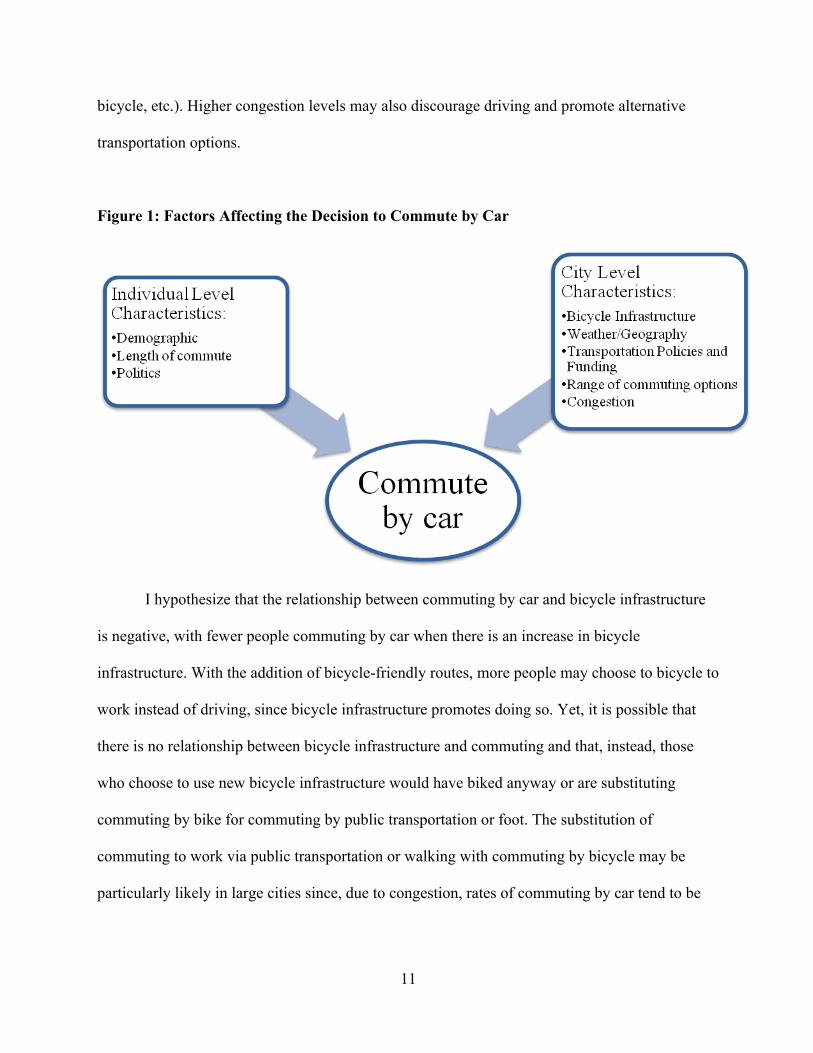
Figure 1 shows factors that, as discussed in the literature review, are related to the
dependent variable, commuting by car, and key independent variable, miles of bicycle
infrastructure per square mile. These can be broken down into two main categories: individual-
level factors and city-level factors. The individual-level characteristics that have an impact on
whether one commutes by car are primarily demographic and include gender, age, race, poverty
status, education, household size, family composition, car ownership, and income. Individual
determinants of commute choice also include the length of one’s commute (since people with
shorter commutes are more likely to not drive to work) and political inclination (more liberal,
environmentally conscious individuals are more likely to commute by bicycle).
City-level factors that influence commute-mode decisions include the availability of
bicycle infrastructure, population size, city size, the existence of bicycle-friendly policies,
transportation funding levels, safety, and gas prices. A city’s weather and geography also play
roles, with factors like cold and hot weather days, precipitation levels, steepness of the roads (or
bike paths), and concentration of residential, commercial, and other properties in a central
location influencing commute choices. Additionally, commuting choices are related to the range
of available commuting alternatives (i.e., driving, taking public transportation, walking, riding a
11
bicycle, etc.). Higher congestion levels may also discourage driving and promote alternative
transportation options.
Figure 1: Factors Affecting the Decision to Commute by Car
I hypothesize that the relationship between commuting by car and bicycle infrastructure
is negative, with fewer people commuting by car when there is an increase in bicycle
infrastructure. With the addition of bicycle-friendly routes, more people may choose to bicycle to
work instead of driving, since bicycle infrastructure promotes doing so. Yet, it is possible that
there is no relationship between bicycle infrastructure and commuting and that, instead, those
who choose to use new bicycle infrastructure would have biked anyway or are substituting
commuting by bike for commuting by public transportation or foot. The substitution of
commuting to work via public transportation or walking with commuting by bicycle may be
particularly likely in large cities since, due to congestion, rates of commuting by car tend to be
12
lower than the national average and point-to-point commuting by bicycle is often faster and more
convenient than commuting on foot or by public transportation.
DATA AND METHODS
This analysis uses a city-year panel dataset constructed using data from several different
sources. Data on the dependent variable, percentage of commuters travelling by car, is available
through the American Community Survey (ACS), a continuous Census Bureau survey that
samples a portion of the U.S. population annually and contains a wide range of information
related to respondents’ demographic characteristics. Federal and state officials use these data to
allocate government resources. The ACS includes single-year, three-year, and five-year
estimates that represent data collected over differing periods of time. To ensure an apples-to-
apples comparison for the city-years of interest, this analysis uses one-year estimates, the data for
which are collected over 12 months in areas with populations over 65,000.
Very little data exist for the key independent variable, miles of bicycle infrastructure, and
what data there are were not collected by a government agency. There is one reasonably reliable
source: the Alliance for Bicycling and Walking (ABW), which operates a biannual
benchmarking project funded by the Centers for Disease Control and Prevention, American
Association of Retired Persons, and Planet Bike. These data are available for 2007, 2009, and
2011 and include city-level information on infrastructure and transportation spending for the 51
largest U.S. cities in a given year. They are collected through two surveys that reach out to city
staff, state Departments of Transportation, metropolitan planning organizations, and advocacy
organizations. The dependent variable for the regressions, bicycle lane miles per square mile,
was created by dividing each city-year’s estimated number of miles of bicycle infrastructure by
13
the city’s square miles as collected by the ABW survey to ensure an apples-to-apples
comparison.2
My initial sample size was 153: 51 cities for three years. In 2007, ABW was unable to
obtain data from nine of the 51 cities, bringing the sample size down to 144. Also, in 2007 ABW
collected data from Amarillo, Texas but did not collect data from that city in any other years,
therefore it was excluded from the final dataset because in order to be included in my fixed
effects models, I require at least two data points for each city. The final sample size is 143 city-
year observations.
All monetary variables, including median household income and state average annual gas
price, were inflation adjusted to 2011 dollars using the average Consumer Price Index for a given
calendar year as determined by the U.S. Department of Labor Bureau of Labor Statistics.
This analysis uses Ordinary Least Squares (OLS) regression with city and year fixed
effects. The fixed effects specification controls for static unobserved characteristics unique to a
particular city as well as for time-varying unobserved characteristics common to all cities in a
given year. This technique reduces the potential for omitted variable bias in the model’s
parameter estimates. Per the discussion in the literature review and conceptual framework, the
time varying control variables summarized in Table 1 below are plausibly correlated with miles
of bicycle infrastructure and the rate of commuting by car. These variables are included in the
model to in order to further reduce omitted variable bias.
2 City size in square miles as reported in the 2000 Census was used for the the 2007 and 2009 ABW Surveys while city size in square miles as reported in the 2010 Census was used for the 2011 ABW Survey. The boundary lines and metropolitan areas of several cities changed significantly and so are included as a control.

14
The equation for the regression can be expressed as:
The alpha term represents city fixed effects and the gamma term represents year fixed effects.
The i subscript refers to the “ith” city and the subscript t refers to the “tth” year.
Many of the determinants of commute mode choice are difficult to measure and were
therefore operationalized using proxies. To operationalize weather, I include the number of days
with greater than .1 inches of precipitation. Economic determinants of commute choice are
operationalized using state average gas price. To control for ideological factors that could
influence commute mode choice, I include a measure from the League of Conservation Voters
that ranks members of Congress from 0 to 100 based on environmental and conservation-related
voting records. While congressional districts do not correspond exactly to city boundary lines,
this measure approximates the ideological makeup of a particular area. To control for safety-
related considerations, I include measures of bicycle fatalities per year and property crime rates.
To control for the availability of public transit, I use a measure of the public transit miles
travelled per year divided by the population. To control for congestion, I include a measure of
the ratio of the travel time during the peak period to the time required to make the same trip at
free-flow speeds. I also include a variety of demographic characteristics to account for their
possible influences on the dependent and key independent variables.

15
Variable Name Definition* Source
Percentage Commuting by Car
The percentage of the commuting population who commute by car
ACS
Miles of Bicycle Infrastructure Per Square Mile
Miles of on-street bike lanes, multiuse and bike paths, and signed bike routes divided by city square miles ABW
Population City population in 100,000s ACSCity Size Size of each city in miles squared in 1,000s ABW
Days with greater than .1 inch of precipitation
The number of days per year where precipitation was greater one-tenth of one inch
National Oceanic and Atmonspheric Administration
EnvironmentalismScore of how members of Congress vote on environmental and conservation issues with 100 as the most supportive and 0 as the least
League of Conservation Voters
Property Crime Rate Rate of crime including burgularies, larceny, and motor vehicle theft
Federal Bureau of Investigation**
Bicycle Fatalities Number of bicycle deaths per year ABW
State Average Gas Price Average price of gas within a state, inflation adjusted to 2011 dollars
Energy Information Administration
Miles of Public Transportation Travelled Per Person
Total miles of public transportation traveled divided by population
National Transit Database
Congestion The ratio of the travel time during the peak period to the time required to make the same trip at free-flow speeds
Texas Transportation Institute
Proportion of Commuters who Walk
Proportion of commuting population who walk to work ACS
Mean Commute Time Mean length of commute in time ACSMale Proportion of Population
Proportion of the population that is male ACS
Nonwhite Proportion of Population
Proportion of population that identifies as nonwhite, incuding black, asian, native american, pacific islander, and multiple races
ACS
Average Household Size Average number of people in a household ACSProportion of Households with a Child under 18
Proportion of households that include a child under the age of 18 ACS
Median Household Income Median income of households inflation adjusted to 2011 dollars ACSMedian Household Income Squared
Median income of households inflation adjusted to 2011 dollars squared
Calculation
Percentage High School Graduates
Percentage of the over 25 population who have graduated from high school
ACS
Percentage Bachelor's Degree or Higher
Percentage of the over 25 population who have a Bachelor's degree or higher ACS
* All variables are continuous** Data for Chicago, Honolulu, Kansas City, and Tuscon were collected directly from Police Department websites
Table 1: Variable Definitions
Dependent Variable
Key Independent Variable
City Level Controls
Individual Level Controls
16
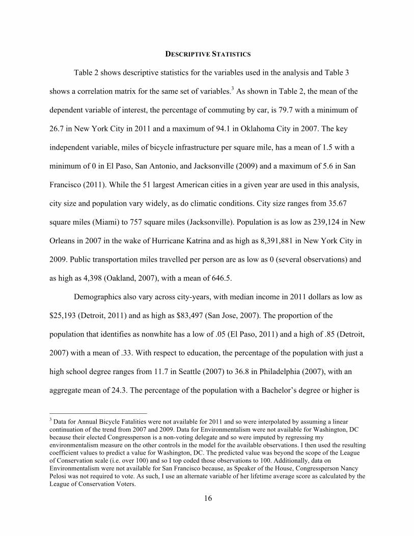
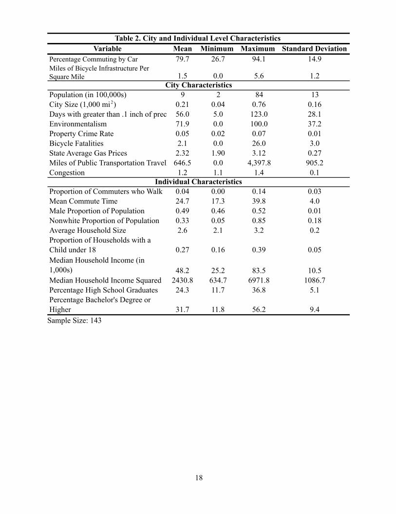
DESCRIPTIVE STATISTICS
Table 2 shows descriptive statistics for the variables used in the analysis and Table 3
shows a correlation matrix for the same set of variables.3 As shown in Table 2, the mean of the
dependent variable of interest, the percentage of commuting by car, is 79.7 with a minimum of
26.7 in New York City in 2011 and a maximum of 94.1 in Oklahoma City in 2007. The key
independent variable, miles of bicycle infrastructure per square mile, has a mean of 1.5 with a
minimum of 0 in El Paso, San Antonio, and Jacksonville (2009) and a maximum of 5.6 in San
Francisco (2011). While the 51 largest American cities in a given year are used in this analysis,
city size and population vary widely, as do climatic conditions. City size ranges from 35.67
square miles (Miami) to 757 square miles (Jacksonville). Population is as low as 239,124 in New
Orleans in 2007 in the wake of Hurricane Katrina and as high as 8,391,881 in New York City in
2009. Public transportation miles travelled per person are as low as 0 (several observations) and
as high as 4,398 (Oakland, 2007), with a mean of 646.5.
Demographics also vary across city-years, with median income in 2011 dollars as low as
$25,193 (Detroit, 2011) and as high as $83,497 (San Jose, 2007). The proportion of the
population that identifies as nonwhite has a low of .05 (El Paso, 2011) and a high of .85 (Detroit,
2007) with a mean of .33. With respect to education, the percentage of the population with just a
high school degree ranges from 11.7 in Seattle (2007) to 36.8 in Philadelphia (2007), with an
aggregate mean of 24.3. The percentage of the population with a Bachelor’s degree or higher is
3 Data for Annual Bicycle Fatalities were not available for 2011 and so were interpolated by assuming a linear continuation of the trend from 2007 and 2009. Data for Environmentalism were not available for Washington, DC because their elected Congressperson is a non-voting delegate and so were imputed by regressing my environmentalism measure on the other controls in the model for the available observations. I then used the resulting coefficient values to predict a value for Washington, DC. The predicted value was beyond the scope of the League of Conservation scale (i.e. over 100) and so I top coded those observations to 100. Additionally, data on Environmentalism were not available for San Francisco because, as Speaker of the House, Congressperson Nancy Pelosi was not required to vote. As such, I use an alternate variable of her lifetime average score as calculated by the League of Conservation Voters.
17
as low as 11.8 in Detroit (2007) and as high as 56.2 in Seattle (2011), with an aggregate mean of
31.7.
Commute characteristics also vary. The proportion of commuters who walk to work has a
mean of .04, a low of 0 (Jacksonville, 2011), and a high of .14 (Boston, 2011). Mean commute
time in minutes is as low 17.3 minutes (Omaha, 2007) and as high as 39.8 (New York, 2007),
with an aggregate mean of 24.7.
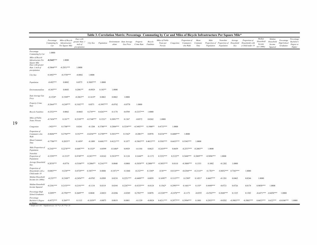
Table 3 shows a correlation matrix of the variables used in this analysis. The correlation
between the independent variable of interest and the dependent variable is -0.34. This
relationship is statistically significant at the 99% level and indicates that there is a negative
relationship between cities’ bicycle infrastructure per square mile and the rate of commuting by
car, as hypothesized. This relationship is only correlational and the fixed effects and regular
regressions in the next section explore this relationship in a more sophisticated fashion.
18
Sample Size: 143
Variable Mean Minimum Maximum Standard DeviationPercentage Commuting by Car 79.7 26.7 94.1 14.9Miles of Bicycle Infrastructure Per Square Mile 1.5 0.0 5.6 1.2
Population (in 100,000s) 9 2 84 13City Size (1,000 mi2) 0.21 0.04 0.76 0.16Days with greater than .1 inch of precipitation56.0 5.0 123.0 28.1Environmentalism 71.9 0.0 100.0 37.2Property Crime Rate 0.05 0.02 0.07 0.01Bicycle Fatalities 2.1 0.0 26.0 3.0State Average Gas Prices 2.32 1.90 3.12 0.27Miles of Public Transportation Travelled Per Person646.5 0.0 4,397.8 905.2Congestion 1.2 1.1 1.4 0.1
Proportion of Commuters who Walk 0.04 0.00 0.14 0.03Mean Commute Time 24.7 17.3 39.8 4.0Male Proportion of Population 0.49 0.46 0.52 0.01Nonwhite Proportion of Population 0.33 0.05 0.85 0.18Average Household Size 2.6 2.1 3.2 0.2Proportion of Households with a Child under 18 0.27 0.16 0.39 0.05Median Household Income (in 1,000s) 48.2 25.2 83.5 10.5Median Household Income Squared 2430.8 634.7 6971.8 1086.7Percentage High School Graduates 24.3 11.7 36.8 5.1Percentage Bachelor's Degree or Higher 31.7 11.8 56.2 9.4
City Characteristics
Individual Characteristics
Table 2. City and Individual Level Characteristics
Percentage
Commuting by Car
Miles of Bicycle Infrastructure
Per Square Mile
Days with greater than .1
inch of precipitation
City Size PopulationEnvironment-
alismState Average
Gas PriceProperty
Crime RateBicycle
Fatalities
Miles of Public Trans per Person
CongestionProportion of Commuterswho Walk
Mean Commute
Time
Male Proportion of
Population
Nonwhite Proportion of
Population
Average Household
Size
Proportion of Households with a Child under 18
Median Household
Income (in 1,000s)
Median Household
Income Squared
Percentage High School Graduates
Percentage Bachelor's Degree or
Higher
Percentage Commuting by Car
1.0000
Miles of Bicycle Infrastructure Per Square Mile
-0.3443*** 1.0000
Days with greater than .1 inch of precipitation
-0.3064*** -0.2931*** 1.0000
City Size 0.3492*** -0.3758*** -0.0882 1.0000
Population -0.492*** 0.0082 0.0575 0.3085*** 1.0000
Environmentalism -0.365*** 0.0603 0.2081** -0.0929 0.183** 1.0000
State Average Gas Price
-0.1528* 0.1949** -0.2063** -0.1619* 0.0063 0.0063 1.0000
Property Crime Rate
.0.2664*** -0.249*** 0.3182*** 0.0571 -0.3997*** -0.0742 -0.0770 1.0000
Bicycle Fatalities -0.2523*** 0.0062 -0.0683 0.274*** 0.6263*** 0.1174 0.0709 -0.2337*** 1.0000
Miles of Public Trans /Person
-0.7434*** 0.181** 0.2338*** -0.3748*** 0.1531* 0.3091*** 0.156* -0.0572 0.0262 1.0000
Congestion -.5425*** 0.1708*** 0.0241 -0.1284 0.3780*** 0.2884*** 0.3254*** -0.3492*** 0.1900** 0.4733*** 1.0000
Proportion of Commuters who Walk
-0.8684*** 0.2794*** 0.352*** -0.4256*** 0.2709*** 0.3033*** 0.1562* -0.2081** 0.0978 0.6234*** 0.4480*** 1.0000
Mean Commute Time
-0.7706*** 0.2035** 0.1459* -0.1089 0.6681*** 0.4121*** 0.1077 -0.3863*** 0.4013*** 0.5585*** 0.6655*** 0.5545*** 1.0000
Male Proportion of Population
0.2343*** 0.2278*** -0.4487*** 0.1525* -0.0599 -0.1484* 0.0929 -0.1184 0.0623 -0.2419*** 0.0659 -0.2537*** -0.2003** 1.0000
Nonwhite Proportion of Population
-0.3295*** -0.1515* 0.4749*** -0.2437*** -0.0162 0.3819*** 0.1124 0.1644** -0.1172 0.3252*** 0.2122** 0.3648*** 0.2889*** -0.5096*** 1.0000
Average Household Size
0.2874*** -0.0776 -0.5104*** 0.2084** 0.2163*** 0.0040 -0.0001 -0.3838*** 0.2408*** -0.3055*** 0.0110 -0.3088*** 0.1333 0.1082 -0.1202 1.0000
Proportion of Households with a Child under 18
0.6083*** -0.234*** -0.4729*** 0.3457*** 0.0880 -0.1871** -0.1068 -0.232*** 0.1389* -0.56*** 0.0110*** -0.6384*** -0.2116** 0.1783** -0.4052*** 0.7365*** 1.0000
Median Household Income (in 1,000s)
-0.235*** 0.2108** -0.2454*** -0.0785 0.0509 0.0218 0.2251*** -0.4409*** 0.0059 0.1699** 0.3115*** 0.1589* 0.1451* 0.4607*** -0.1281 0.0465 0.0246 1.0000
Median Household Income Squared
-0.2381*** 0.2155*** -0.2191*** -0.1134 0.0319 0.0344 0.2287*** -0.4335*** -0.0124 0.1562* 0.2995*** 0.1681** 0.155* 0.4449*** -0.0721 0.0726 0.0174 0.9858*** 1.0000
Percentage High School Graduates
0.2095** -0.3705*** 0.2689*** 0.0840 -0.0033 -0.0286 -0.0385 0.2703*** 0.0078 -0.2328*** -0.2478*** -0.1173 -0.0355 -0.4765*** 0.2848*** 0.1325 0.1303 -0.6471*** -0.6058*** 1.0000
Percentage Bachelor's Degree or Higher
-0.4572*** 0.269*** 0.1115 -0.1839** -0.0075 0.0819 0.0801 -0.1339 -0.0824 0.4211*** 0.2977*** 0.3994*** 0.1001 0.2935*** -0.0282 -0.5083*** -0.5083*** 0.6653*** 0.622*** -0.8106*** 1.0000
* Sample size=143. * Significant at p<.10, ** p<.05, ***p<.01
Table 3. Correlation Matrix: Percentage Commuting by Car and Miles of Bicycle Infrastructure Per Square Mile*
19

20
REGRESSION RESULTS
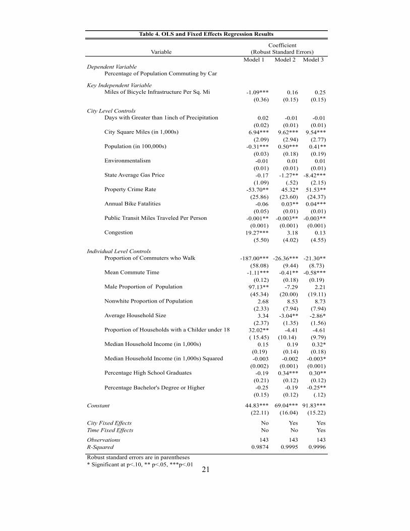
Table 4 presents estimated regression coefficients for three different regression models.
Robust standard errors are reported in parentheses immediately below each coefficient. The
column marked “Model 1” contains the results from a model that contains a full set of controls
but does not use fixed effects. The column marked “Model 2” shows results from a model using
city fixed effects. The column labeled “Model 3” shows results from a model using city and year
fixed effects. The control variables are grouped into city- and individual-level characteristics. As
explained in the Data and Methods section, the control variables account for time varying
characteristics that may be correlated with the dependent and/or key independent variable.
The availability of many different measures of the same basic variables required a
determination as to which was the most sensible to include. I estimated models using alternative
measures for several broad categories. The final model allows me to capture the dynamics for
which I wish to control in the most parsimonious way.4
4 I estimated models using several different measures of climate, commute characteristics, demographics, and safety and then evaluated their relative statistical significance, magnitude, and effect on the key independent variable coefficient. For climate, I estimated models including heating degree days, cooling degree days, days with one inch of snow or more, days with .1 inch of precipitation or more, and days with .5 inch of precipitation or more. For commute characteristics, I estimated models including measures of the proportion of the population with a variety of commute time lengths in minutes, including under 10, 10-14, 15-19, 20-24, 25-29, 30-34, 25-44, 45-59, under 30, over 60, and mean commute time. For availability of public transit, I estimated models including the proportion of commuters who take public transit and the number of transit miles traveled per person. For education, I estimated models using several different measures, including percentage of the population 25 and older with less than a high school degree, high school degree only, some college, associate’s degree, bachelor’s degree, post-graduate degree, high school or higher, and bachelor’s degree or higher. In terms of household composition, I estimated models using average household size and average family size as well as proportion of married households, proportion of single person households, proportion of households with a child six or younger, and proportion of households with a child 18 or younger. In terms of demographic controls, I estimated models using several different race and poverty measures. For safety measures, I evaluated models including property crime rates and violent crime rates as well as annual bicyclist fatalities. The final variables in the model were included based on their influence on the coefficient for the key independent variable relative to the other options available. In other words, I included all variables whose omission would have induced bias in the coefficient of interest.
21
Model 1 Model 2 Model 3Dependent Variable
Percentage of Population Commuting by Car
Key Independent VariableMiles of Bicycle Infrastructure Per Sq. Mi -1.09*** 0.16 0.25
(0.36) (0.15) (0.15)
City Level ControlsDays with Greater than 1inch of Precipitation 0.02 -0.01 -0.01
(0.02) (0.01) (0.01)City Square Miles (in 1,000s) 6.94*** 9.62*** 9.54***
(2.09) (2.94) (2.77)Population (in 100,000s) -0.31*** 0.50*** 0.41**
(0.03) (0.18) (0.19)Environmentalism -0.01 0.01 0.01
(0.01) (0.01) (0.01)State Average Gas Price -0.17 -1.27** -8.42***
(1.09) (.52) (2.15)Property Crime Rate -53.70** 45.32* 51.53**
(25.86) (23.60) (24.37)Annual Bike Fatalities -0.06 0.03** 0.04***
(0.05) (0.01) (0.01)Public Transit Miles Traveled Per Person -0.001** -0.003** -0.003**
(0.001) (0.001) (0.001)Congestion 19.27*** 3.18 0.13
(5.50) (4.02) (4.55)
Individual Level ControlsProportion of Commuters who Walk -187.00*** -26.36*** -21.30**
(58.08) (9.44) (8.73) Mean Commute Time -1.11*** -0.41** -0.58***
(0.12) (0.18) (0.19) Male Proportion of Population 97.13** -7.29 2.21
(45.34) (20.00) (19.11)Nonwhite Proportion of Population 2.68 8.53 8.73
(2.33) (7.94) (7.94)Average Household Size 3.34 -3.04** -2.86*
(2.37) (1.35) (1.56)Proportion of Households with a Childer under 18 32.02** -4.41 -4.61
( 15.45) (10.14) (9.79)Median Household Income (in 1,000s) 0.15 0.19 0.32*
(0.19) (0.14) (0.18)Median Household Income (in 1,000s) Squared -0.003 -0.002 -0.003*
(0.002) (0.001) (0.001)Percentage High School Graduates -0.19 0.34*** 0.30**
(0.21) (0.12) (0.12)Percentage Bachelor's Degree or Higher -0.25 -0.19 -0.25**
(0.15) (0.12) (.12)
Constant 44.83*** 69.04*** 91.83***(22.11) (16.04) (15.22)
City Fixed Effects No Yes YesTime Fixed Effects No No Yes
Observations 143 143 143R-Squared 0.9874 0.9995 0.9996
Robust standard errors are in parentheses* Significant at p<.10, ** p<.05, ***p<.01
Table 4. OLS and Fixed Effects Regression Results
VariableCoefficient
(Robust Standard Errors)

22
Model 1 indicates that, for each additional mile of bicycle infrastructure per square mile,
the percentage of commuters who travel by car decreases by 1.09 percentage points. This finding
is statistically significant at the 0.01 level. The coefficients in Models 2 and 3 are imprecisely
estimated, as indicated by their low t-values and large standard errors, and are smaller in
magnitude than that in Model 1.
Focusing on Models 2 and 3, the city fixed effects dummies explain almost all of the
variation in the dependent variable. When the percentage of commuters by car is regressed only
on the city fixed effects, the city dummy variables account for over 99% of the variation in
percentage of commuters by car, leaving less than 1% to be explained by bicycle infrastructure
per square mile and all of the additional control variables. Ultimately, due to the small sample
size and limited range of years of data available, there is very little within-city variation in the
dependent variable over time, and the fixed effects dummies capture almost all of the variation
that exists. This suggests that the non-fixed effects regression results may be more reliable, since
they leave a larger portion of the variation in the dependent variable to be explained by the
covariates in the model. However, the amount of variation left unexplained in the regular
regression model is quite low as well, with a regression including just the control variables and
no fixed effects dummies explaining 98.6% of the variation in the dependent variable.
Exploratory analysis showed that the inclusion of population size in the models accounts
for nearly all of the high R-Squared values. Population size is strongly correlated with the
percentage of the population commuting by car and is almost certainly also correlated with the
number of bicycle infrastructure miles per square mile, so it would not be appropriate to exclude
it from this analysis, as doing so would produce omitted variable bias. Nonetheless, its inclusion
23
in the model accounts for almost all of the variation in the percentage of commuters who drive,
leaving very little to be explained by the other variables. Therefore, I estimated regular
regression models without population as a covariate, without population weights, and without
population as a covariate and population weights. The results of these alternate specifications
with respect to the magnitude and significance of the coefficient on the key independent variable
are very similar to those in Model 1. This reveals that, when the main driver of the high R-
Squared value of the non-fixed effects regression is excluded, the coefficient on the key
independent variable is still small but statistically significant, indicating that results are not being
driven solely by the limited variation in the dependent variable.
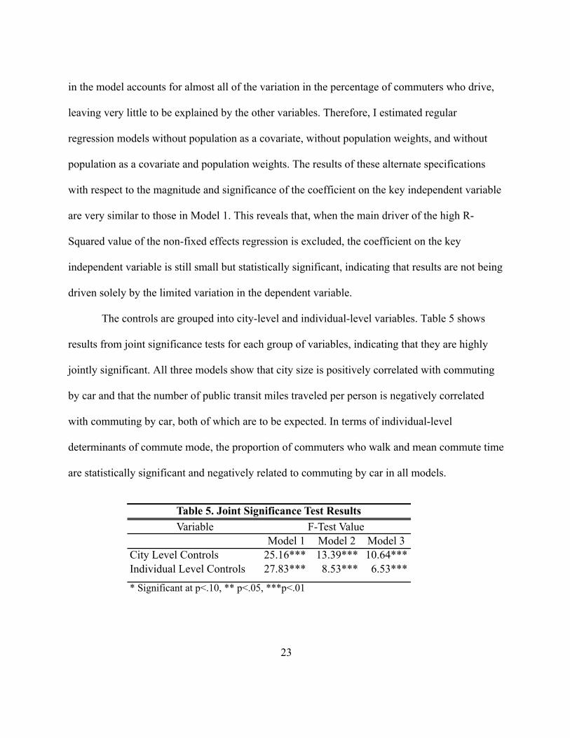
The controls are grouped into city-level and individual-level variables. Table 5 shows
results from joint significance tests for each group of variables, indicating that they are highly
jointly significant. All three models show that city size is positively correlated with commuting
by car and that the number of public transit miles traveled per person is negatively correlated
with commuting by car, both of which are to be expected. In terms of individual-level
determinants of commute mode, the proportion of commuters who walk and mean commute time
are statistically significant and negatively related to commuting by car in all models.
VariableModel 1 Model 2 Model 3
City Level Controls 25.16*** 13.39*** 10.64***Individual Level Controls 27.83*** 8.53*** 6.53***
* Significant at p<.10, ** p<.05, ***p<.01
F-Test ValueTable 5. Joint Significance Test Results

24
Overall, these results yield three interesting findings. First, city size in square miles,
public transportation miles traveled per person, proportion of commuters who walk, and mean
commute time are statistically significant correlates of commuting by car in all models. Thus,
commuting options and city-level characteristics appear to have the strongest relationship with
commute mode choice. Second, arguably, Model 1 most usefully assesses the relationship
between the dependent variable and key independent variable because there is such limited
variation in the fixed effects models from which to estimate a relationship. Third, Model 1 shows
a statistically significant negative relationship between bicycle infrastructure and commuting by
car, as hypothesized.
DISCUSSION
The purpose of this study was to determine whether or not there is a relationship between
bicycle infrastructure and commuting by car in large American cities. Logically, one might think
that increasing the availability of bicycle-specific travel options would reduce the percentage of
people who drive to work, but it is unclear whether people who choose to bicycle to work would
otherwise drive.
All three models show a relationship so small as to be negligible between bicycle
infrastructure and the rate of commuting by car. Only one regression shows a statistically
significant and negative relationship between bicycle infrastructure and the rate of commuting by
car. The models incorporating city and year fixed effects show a weak positive relationship that
is not statistically different from zero. Model 1, using regular OLS regression, shows a somewhat
less weak and statistically significant negative association, whereby the addition of one mile of
25
bicycle infrastructure per square mile is associated with a one percentage point reduction in the
percent commuting by car. This is quite a small change, as the mean percent commuting by car is
80 and the mean number of miles of bicycle infrastructure per square mile is 1.5. Thus,
increasing the existing bicycle infrastructure by 67% is associated with 1% decrease in
commuting by car.
For the fixed effects models, it should be remembered that city and year fixed effects
control for the vast majority of the variation in the dependent variable, leaving very little to be
explained by the independent variable of interest. Thus, the regular OLS model may capture
better the relationship between commuting by car and bicycle infrastructure, since there is
slightly more variation left to be explained. Also, excluding the key driver of the high R-Squared
value, thereby freeing up more variation in the data, had very similar results. Importantly, even
though the relationship is statistically significant in Model 1, it is still miniscule.
There are also significant limitations to this analysis. Data on the independent variable of
interest, miles of bicycle infrastructure per square mile, are available only from one source and
only for three years. These data are also not available for all cities in all three years, further
limiting variation in the dependent variable over time. Data from more cities and over a longer
time period would offer richer variation in the dependent variable and key independent variable
to be explored in subsequent research and therefore would provide a more complete picture of
the true relationship between bicycle infrastructure and commuting by car. These data are also
reported by city governments and so are not collected in a standardized fashion. Having data
collected in a uniform way would improve future inquiries in this area.
26
Moreover, there is the distinct possibility of omitted variable bias in this analysis. While
the fixed effects models mitigate a great deal of potential bias, there are other possible influences
on commute mode choice that were not included in these models and could be explored in future
research. One such variable is the availability of bikeshare programs, in which an individual pays
a fee to collect a bicycle from a station and returns that bicycle to any other station within the
service area, with additional pricing based on use time. These programs have changed the
landscape of bicycle use in cities by providing a new convenient, fast, and inexpensive non-
motorized point-to-point transport option. Specifically, in 2009, the city of Paris found that 28%
of respondents to a survey about their bikesharing program indicated that they were less likely to
use personal vehicles in 2008 due to the availability of bikes. This figure increased to 46% in
2009 (DeMaio 2009). Bikesharing programs are spreading rapidly throughout the nation, and
including a measure of availability could improve similar models in future analysis.
Additionally, types of bicycle infrastructure, government policies, and program funding
levels may affect commute mode choices. New infrastructure innovations include bike boxes,
which favor cyclists at red lights; cycle tracks, or lanes for cyclists separated from vehicle traffic
by physical barriers; and contra flow bike lanes, which allow cyclists to travel in either direction
on one-way streets (Pucher, Dill, & Handy, 2010). In addition, bicycle-transit integration, such
as having bike racks on buses and allowing bikes on trains, could be an important control
variable for future research, since people may be more willing to take public transit to work
rather than drive if they can cycle to stations (Krizek & Stonebraker, 2011). Complete streets
policies, safe routes to schools, bike to work days, and public information campaigns aimed at
cyclists and drivers could promote greater awareness of transportation alternatives as well as

27
encourage safe driving and cycling (Alliance for Bicycling and Walking, 2012). The policies and
programs above are probably positively related to the presence of bicycle infrastructure and
negatively related to percentage of the population commuting by car, therefore the omission of
these variables from the models likely exerts downward bias on the coefficient for the key
independent variable. The inclusion of variables controlling for program funding levels would
mitigate this downward bias and provide a more accurate causal estimate of the relationship
studied here.
Ultimately, the policy implications of this research are limited. There is a relationship
between bicycle infrastructure and commuting by car in some, but not all, models. Moreover,
this relationship is negligible in magnitude. Because there is modestly more variation to exploit
in the dependent variable, the regular OLS regression model in which there is a statistically
significant relationship is perhaps the most credible of the three models run. This analysis
provides suggestive evidence that there might be such a relationship and that cities seeking to
encourage non-motorized commute to work choices might consider investing more heavily in
bicycle infrastructure. With further research and the collection of more and more accurate data,
policymakers will be better able to more comprehensively evaluate options for the most efficient
use of public funds in order to encourage particular commute mode choices.

28
REFERENCES Alliance for Bicycling and Walking. (2007). Bicycling and Walking in the United States: 2007
Benchmarking Report. Washington, DC: Alliance for Bicycling and Walking.
Alliance for Bicycling and Walking. (2010). Bicycling and Walking in the United States: 2010 Benchmarking Report. Washington, DC: Alliance for Bicycling and Walking.
Alliance for Bicycling and Walking. (2012). Bicycling and Walking in the United States: 2012 Benchmarking Report. Washington, DC: Alliance for Bicycling and Walking.
Bergström, A., & Magnusson, R. (2003). Potential of transferring car trips to bicycle during winter. Transportation Research Part A: Policy and Practice, 37(8), 649-666.
Buehler, R. (2010). Transport policies, automobile use, and sustainable transport: A comparison of Germany and the United States. Journal of Planning Education and Research, 30(1), 76-93.
Buehler, R., & Pucher, J. (2012). Cycling to work in 90 large American cities: New evidence on the role of bike paths and lanes. Transportation, 39(2), 409-432.
Cervero, R., & Duncan, M. (2003). Walking, bicycling, and urban landscapes: Evidence from the San Francisco Bay area. American Journal of Public Health, 93(9), 1478-1483.
City of Tuscon. (2011). Crime Trend Graphs: 1997-2011, Property Crime. Retrieved from City of Tuscon website: http://cms3.tucsonaz.gov/police/crime-trend-graphs
Cooper, A. R., Andersen, L. B., Wedderkopp, N., Page, A. S., & Froberg, K. (2005). Physical activity levels of children who walk, cycle, or are driven to school. American Journal of Preventive Medicine, 29(3), 179-184.
Dargay, J., & Hanly, M. (2007). Volatility of car ownership, commuting mode and time in the UK. Transportation Research Part A: Policy and Practice, 41(10), 934-948.
de Hartog, J. J., Boogaard, H., Nijland, H., & Hoek, G. (2010). Do the health benefits of cycling outweigh the risks? Environmental Health Perspectives, 118(8), 1109.
De Zeeuw, D., & Flusche, D. (2011). How a bill becomes a bike lane: Federal legislation, programs, and requirements of bicycling and walking projects. Planning & Environmental Law, 63(8), 8-11.

29
DeMaio, P. (2009). Bike-sharing: History, impacts, models of provision, and future. Journal of Public Transportation, 12(4), 41-56.
Dill, J., & Carr, T. (2003). Bicycle commuting and facilities in major U.S. cities: If you build them, commuters will use them. Transportation Research Record: Journal of the Transportation Research Board, 1828(-1), 116-123.
Dill, J., & Voros, K. (2007). Factors affecting bicycling demand: Initial survey findings from the Portland, Oregon region. Transportation Research Record: Journal of the Transportation Research Board, 2031(1), 9-17.
Frank, L. D., Andresen, M. A., & Schmid, T. L. (2004). Obesity relationships with community design, physical activity, and time spent in cars. American Journal of Preventive Medicine, 27(2), 87-96.
Frey, W. (2012, June 29). Demographic Reversal: Cities Thrive, Suburbs Sputter. Retrieved from The Brookings Institution, http://www.brookings.edu/research/opinions/2012/06/29-cities-suburbs-frey
Garrard, J., Rose, G., & Lo, S. (2008). Promoting transportation cycling for women: The role of bicycle infrastructure. Preventive Medicine, 46(1), 55-59.
Garrett-Peltier, H. (2010). Estimating the Employment Impacts of Pedestrian, Bicycle, and Road Infrastructure-Case Study: Baltimore. Political Economy Research Institute, University of Massachusetts, Amherst.
Gotschi, T., & Mills, K. (2008). Active Transportation for America: The Case for Increased Federal Investment in Bicycling and Walking. Washington, DC: Rails-to-Trails Conservancy.
Hall, M. L. (2012, June 29). Analysis of the new transportation bill, MAP-21 [Web log message]. Retrieved from America Bikes blog, http://www.americabikes.org/blog
Hartgen, D., & Fields, G. (2006). Building Roads to Reduce Traffic Congestion in America's Cities: How Much and at What Cost? Washington, DC: Reason Foundation.
Honolulu Police Department. (2011). Statistics 2011. Retrieved from the Honolulu Police Department website: http://www.honolulupd.org/downloads/HPD2011annualreportstatistics.pdf

30
Horner, J. (2012). Less driving, more saving: The economic benefits of cutting car travel. Washington, DC: Natural Resources Defense Council.
Illinois State Police. (2009). Crime in Illinois 2009 Annual Uniform Crime Report. Retrieved from the Illinois State Police website: http://www.isp.state.il.us/crime/cii2009.cfm
Jacobsen, P. L. (2003). Safety in numbers: More walkers and bicyclists, safer walking and bicycling. Injury Prevention, 9(3), 205-209.
Kahn, M. E., & Morris, E. A. (2009) Walking the walk: the association between community environmentalism and green travel behavior. Journal of the American Planning Association 75.4: 389-405.
Kansas City Missouri Police Department. (2008). Annual Report. Retrieved from the Kansas City Missouri Police Department website: http://www.kcmo.org/idc/groups/police/documents/police/annual_report_2008.pdf
Krizek, K. J., Barnes, G., & Thompson, K. (2009). Analyzing the effect of bicycle facilities on commute mode share over time. Journal of Urban Planning and Development, 135(2), 66-73.
Krizek, K. J., & Stonebraker, E. W. (2011). Assessing options to enhance bicycle and transit integration. Transportation Research Record: Journal of the Transportation Research Board, 2217(1), 162-167.
League of Conservation Voters. National Environmental Scorecard. Retrieved December 1, 2012 from National Environmental Scorecard Database available: http://scorecard.lcv.org/
Limtanakool, N., Dijst, M., & Schwanen, T. (2006). The influence of socioeconomic characteristics, land use and travel time considerations on mode choice for medium- and longer-distance trips. Journal of Transport Geography, 14(5), 327-341.
Moving Ahead for Progress in the 21st Century Act. Pub. L. 112-141, (2012).
McDonald, N., Brown, A., Marchetti, L., & Pedroso, M. (2011). U.S. school travel, 2009: An assessment of trends. American Journal of Preventive Medicine, 41(2), 146-151.
Ming Wen, L., & Rissel, C. (2008). Inverse associations between cycling to work, public transport, and overweight and obesity: Findings from a population based study in Australia. Preventive Medicine, 46(1), 29-32.

31
National Oceanic and Atmospheric Administration. (2012). Climate Data Online. Available from the National Climatic Data Center. Retrieved November 20, 2012 from http://www.ncdc.noaa.gov/cdo-web/
Nelson, A. C., & Allen, D. (1997). If you build them, commuters will use them: Association between bicycle facilities and bicycle commuting. Transportation Research Record: Journal of the Transportation Research Board, 1578(-1), 79-83.
Plaut, P. (2005). Non-motorized commuting in the U.S. Transportation Research Part D: Transport and Environment, 10(5), 347-356.
Pucher, J., & Buehler, R. (2007). Cycling in Canada and the United States: Why Canadians are so far ahead. Plan Canada, 47(1), 13-17.
Pucher, J., & Buehler, R. (2008). Making cycling irresistible: Lessons from the Netherlands, Denmark and Germany. Transport Reviews, 28(4), 495-528.
Pucher, J., Buehler, R., Merom, D., & Bauman, A. (2011). Walking and cycling in the United States, 2001-2009: Evidence from the National Household Travel Surveys. American Journal of Public Health, 101(S1), S310-7.
Pucher, J., Buehler, R., & Seinen, M. (2011). Bicycling Renaissance in North America? An update and re-appraisal of cycling trends and policies. Transportation Research Part A: Policy and Practice, 45(6), 451-475.
Pucher, J., Dill, J., & Handy, S. (2010). Infrastructure, programs, and policies to increase bicycling: an international review. Preventive Medicine, 50, S106-S125.
Reynolds, C. C. O., Harris, M. A., Teschke, K., Cripton, P. A., & Winters, M. (2009). The impact of transportation infrastructure on bicycling injuries and crashes: A review of the literature. Environmental Health, 8(1), 47.
Safe, Accountable, Flexible, Efficient Transportation Equity Act: A Legacy for Users. Pub. L. 109-59, 119 Stat. 1144 (2005).
Shrank, D., Lomax, T., & Eisele, B. (2011). 2011 Urban Mobility Report. College Station, TX: University Transportation Center for Mobility, Texas Transportation Institute.
32
Tilahun, N. Y., Levinson, D. M., & Krizek, K. J. (2007). Trails, lanes, or traffic: Valuing bicycle facilities with an adaptive stated preference survey. Transportation Research Part A: Policy and Practice, 41(4), 287-301.
U.S Bureau of Labor and Statistics. (2012). Consumer Price Index. Available from CPI Databases, Inflation Calculator. Retrieved November 25, 2012 from http://www.bls.gov/cpi/
U.S. Census Bureau. (2000). U.S. Census. Available from American Fact Finder database. Retrieved November 15, 2012, from http://factfinder2.census.gov.
U.S. Census Bureau (2007). American Community Survey. Available from American Fact Finder database. Retrieved November 15, 2012, from http://factfinder2.census.gov.
U.S. Census Bureau. (2009). American Community Survey. Available from American Fact Finder database. Retrieved November 15, 2012, from http://factfinder2.census.gov.
U.S. Census Bureau. (2010.) U.S. Census. Available from American Fact Finder database. Retrieved November 15, 2012, from http://factfinder2.census.gov.
U.S. Census Bureau. (2011). American Community Survey. Available from American Fact Finder database. Retrieved November 15, 2012, from http://factfinder2.census.gov.
U.S. Department of Justice (2007). Crime in the United States. Available from the Federal Bureau of Investigation website. Retrieved November 28, 2012 from http://www.fbi.gov/about-us/cjis/ucr/crime-in-the-u.s.
U.S. Department of Justice (2009). Crime in the United States. Available from the Federal Bureau of Investigation website. Retrieved November 28, 2012 from http://www.fbi.gov/about-us/cjis/ucr/crime-in-the-u.s.
U.S. Department of Justice (2011). Crime in the United States. Available from the Federal Bureau of Investigation website. Retrieved November 28, 2012 from http://www.fbi.gov/about-us/cjis/ucr/crime-in-the-u.s.
U.S. Department of Transportation. (2009). National Household Travel Survey. Available from the National Household Travel Survey website. Retrieved November 1, 2012 from http://nhts.ornl.gov/
U.S. Department of Transportation. Pedestrian and Bicycle Information Center. (2010). The National Bicycling and Walking Study: 15–Year Status Report. Available from the
33
Pedestrian and Bicycle Information Center. Retrieved October 7, 2013 from http://www.walkinginfo.org/15_year_report/
U.S. Department of Transportation. (2012). National Transit Database. Available from the National Transit Database website. Retrieved December 1, 2012 from http://www.ntdprogram.gov/ntdprogram/
Winters, M., Friesen, M.C., Koehoorn, M., Teschke, K. (2007). Utilitarian bicycling: a multilevel analysis of climate and personal influences. American Journal of Preventive Medicine, 32(1), 52-58.
Yang, Y., Roux, A. D., & Bingham, C. R. (2011). Variability and seasonality of active transportation in USA: Evidence from the 2001 NHTS. International Journal of Behavioral Nutrition and Physical Activity, 8(1), 96.
Zahran, S., Brody, S. D., Maghelal, P., Prelog, A., & Lacy, M. (2008). Cycling and walking: Explaining the spatial distribution of healthy modes of transportation in the United States. Transportation Research Part D: Transport and Environment, 13(7), 462-470.