A C0

,I it

4 OF

I

OPTIMIZATION OF THE ANTENNA PATTERN OF

A PHASED ARRAY WITH FAiLED ELEMENTS ELECTEAPR 033 O

THESIS

Bernard F. Collins II D oCaptain, USAF

_.__.AFIT/GE/ENG/86D-3)4

S,& •I - . . . ... .

5pprwoi for public relecsjiDlstaibutlon Unlimited

DEPARTMENT OF THE AIR FORCE

'I AIR UNIVERSITY', AIR FORCE INSTITUTE OF TECHNOLOGY

Wright-Patterson Air Force Base, Ohio

2 4026

U AF IT/ GE/ENG/86 D-341

DTIC&%ELECTEx •M

NN

OPTIMIZATION OF THE ANTENNA PATTERN OF

A PHASED ARRAY WITH FAILED EL.A:MENTS

THESIS

Bernard F. Collins II

N •Captain, USAF

AFIT/GE/ENG/86D-34

Approved for public release; distribution unlimited

,' -. f ~*: ' *~ ,,~A

i I a i- -- - i - 4I

AFIT/GE/ENG/86 D-34 I

I

OPTIMIZATION OF THE ANTENNA PATTERN OF

A PHASED ARRAY WITH FAILED ELEMENTS

THESIS

Presented to the Faculty of the School of Engineering

H, of the Air Force Institute of Technology

Air University

In Partial Fulfillment of the

Requiements for the Degree of

Master of Science in Electrical Engineering

INSPECTED9

Accesion For

NTIS CRA&IDTIC TABUinarno iaced [.1

Bernard F. Collins II, B.S. Ju.AiIICut.. .

Captain, USAF ...............................D i t , ib ,itio : I

Availability Codes

.1 d/ll- c or

December 1986 Dit'

Approved for public release; distribution unlimited

VI', 1

Preface

The purpose of this study was to find some method of

¶ 'optimizing the far-field pattern of a phased array with

failed elments. The topic was generated by Col. Larry

Sanborn, while he was at Space Division, who was concerned

with the survivability of a phased array antenna aboard a

satellite. The problem was further defined by Mr. John

McNamara of the Space Based Radar Branch, Rome Air

Development Center, Rome, New York.

At the beginning of the study, I hoped that any

optimization method found would be easily implemented, that

a black box could be built which would have as its imput the

coordimates of the failed element, and as its output the

new, optimized array current amplitude and phase

2 distribtion. The result of this quest is called the direct

method. However, the direct method is not yet ready to be

molded into a black box, for the study done was largely

Stheoretical. I believe the direct method has strong

potential and sl ould be modified for a practical array.

I would like to thank Dr. Andrew Terzuoli for patiently

answering my questions even when he was incredibly busy

- (always), for helping me find either the information I

needed to solve a problem or the experts who might already

have the answer, and for his personal dedication; Lt Ccl

Zdzislaw Lewantowicz for teaching me all about gradienG

k%7

searches and eigenvalues and for all the time he spent

4 1 trying to find the answer on his own; Dr. Vittal Pyati and

Maj Glenn Prescott for their assistance and interest; and

Sue for her love, her level of to.1erance, and her

'II

4_ encouragements.

A •<

4

CfX Kii

................................ ' N~ V~'I&

Table of Contents

Page

Preface . ii

List of Figures ..... .................... v!

List of Tables . . . .. . . . . . . . . . . . viil

Abstract . . . . .. . . . o. x

I. Introduction .*.. . . . . . . . . . . . ..

Background . . . . . . . . . . . . 2Assumptions . .. ............. 2Approach ............ 3Order of Presentation ........... 5

SII . Basic Array Analysis Techniq. ues . . . . . . .. 7

Fourier Transfovm . . . . . . . . . . .. . 9

z,-Transform ......... ................ 10

III. Optimization Techniques..........15

Thinned Array Inalysis . . . .. . 15Description . .. .. ......... 15Application ........ ............ .. 17Results .................... . . . . 21

Adaptive Array Analysis .......... . . 21Description ...... .. ............ 22Application.... . ............. 25Results . . .. ......... . . 28

Eigenvalue Methods a...........29Description .. ..... .. ............ 29Application ......................... 33Results. ... .. ............ . .. 43...-

SNull Displacement Technique ....... ........ L;'4Description............................ 1l44Application . . . . . . . . . . . . . 46Rfesults .... ............... 54

Iterative Techniques .......... ........... 54Description .......... .......... .. 55Application ............... 57Results ........ .............. 65

iv

I MZ- 4 .• . . ., . . ...... ,• -

Direct Technique . . . . . . . .. . 66Description ..... ............. .. 66Application . ............. 68Results . . . . . . . . . . . .. . . TO

IV. Conclusions and Recommendations . . . . . . . . 72

Conclusions . . . . . . . ......... 72Recommendations ...... ...... .. . . . . . 73

Bibliography ........ .... . . . ...... 75

,, Vita ......................... 77

4-

A.'

*4,r

-*-.* .* . -- *. . *. " *'. .- -.OWN. - - *

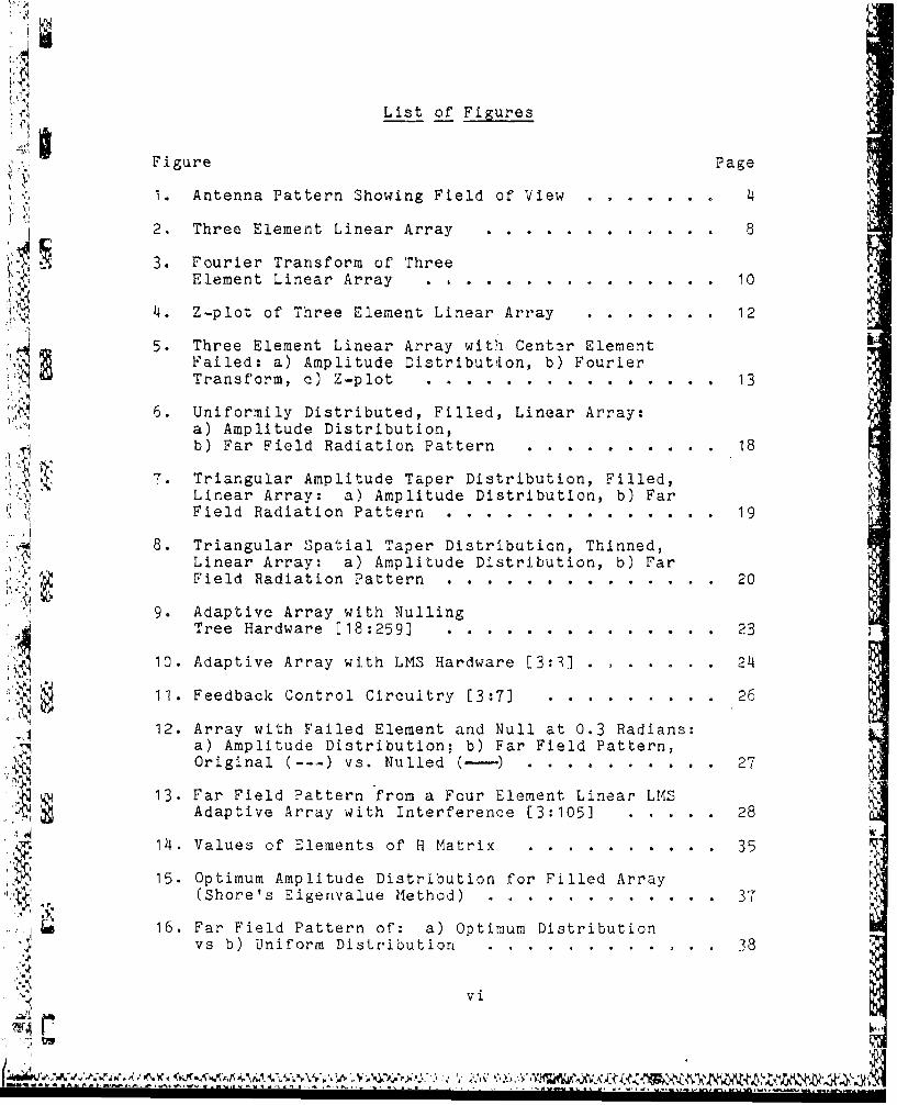
List of Figures

Figure Page

i. Antenna Pattern Showing Field of View ... ........ 4

2. Three Element Linear Array ......... ............ 8

3. Fourier Transform of ThreeElement Linear Array . ............. .... 10

14. Z-plot of Three Element Linear Array ............. 12

5. Three Element Linear Array with Cent3r ElementFailed: a) Amplitude Distribution, b) FourierTransform, c) Z-plot ..... ............ . .. 13

6. Uniformily Distributed, Filled, Linear Array:a) Amplitude Distribution,b) Far Field Radiation Pattern ..... .......... .. 18

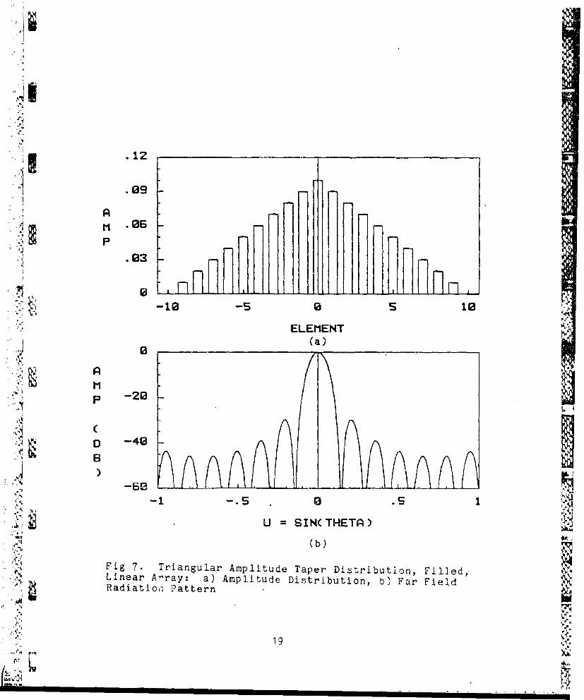
7. Triangular Amplitude Taper Distribution, Filled,Linear Array: a) Amplitude Distribution, b) FarField Radiation Pattern ........ ............. . 19

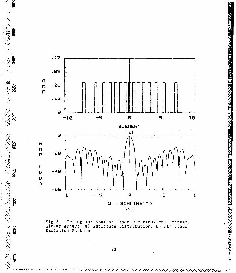
8. Triangular Spatial Taper Distribution, Thinned,Linear Array: a) Amplitude Distribution, b) FarField Radiation Pattern . . ............. 20

9. Adaptive Array with Nulling•Tree Hardware [18:259] . . . . . . . . •..... 23

10. Adaptive Array with LMS Hardware [3:.] .......... 24

11. Feedback Control Circuitry [3:71 ................. 26

12. Array with Failed Element and Null at 0.3 Radians:1a) Amplitude Distribution: b) Far Field Pattern,

Original (---) vs. Nulled (--). .... .......... 27

13. Far Field Pattern from a Four Element Linear LMSAdaptive Array with Interference [3:105] ..... .. 28

14. Values of Elements of H Matrix ... .......... 35

15. Optimum Amplitude Distribution for Filled Array(Shore's Eigenvalue Method) .... ............ 37

16. Far Field Pattern of: a) Optimum Distributionvs b) Uniform Distribution ......... ............ 38

vi

,v

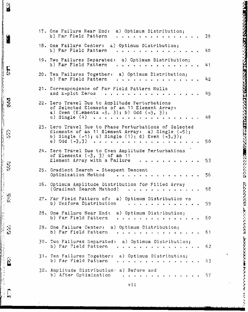
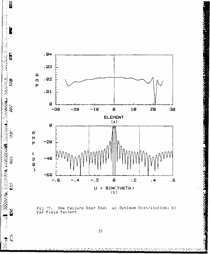
17. One Failure Near End: a) Optimum Distribution;b) Far Field Pattern ................ . ..... . .. 39

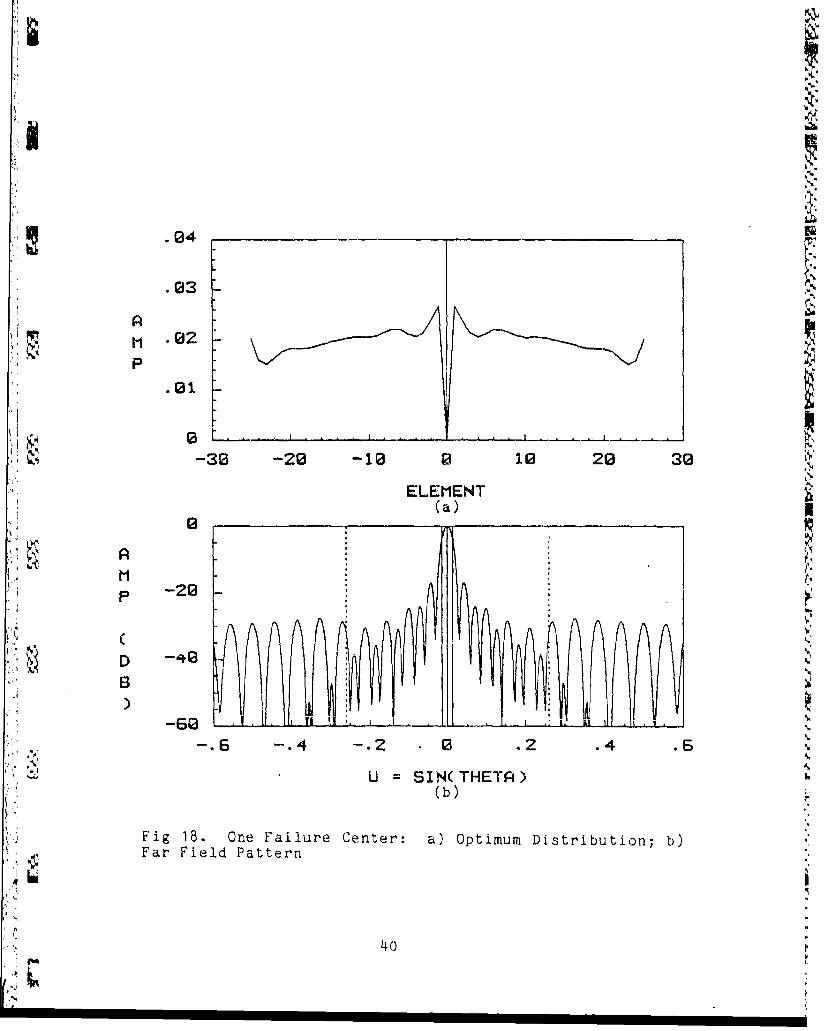
18. One Failure Center: a) Optimum Distribution;b) Far Field Pattern ....... ............... 40

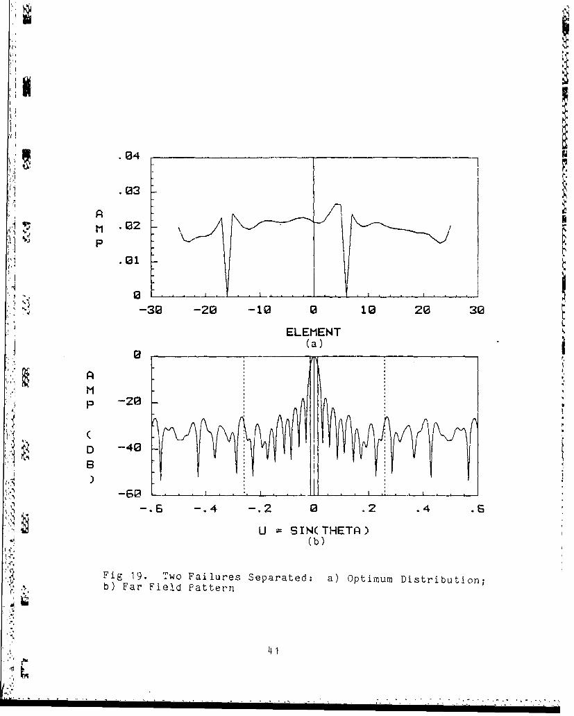
19. Two Failures Separated: a) Optimum Distribution;b) Far Field Pattern . . . . .. *. . . . . . . .* . 41

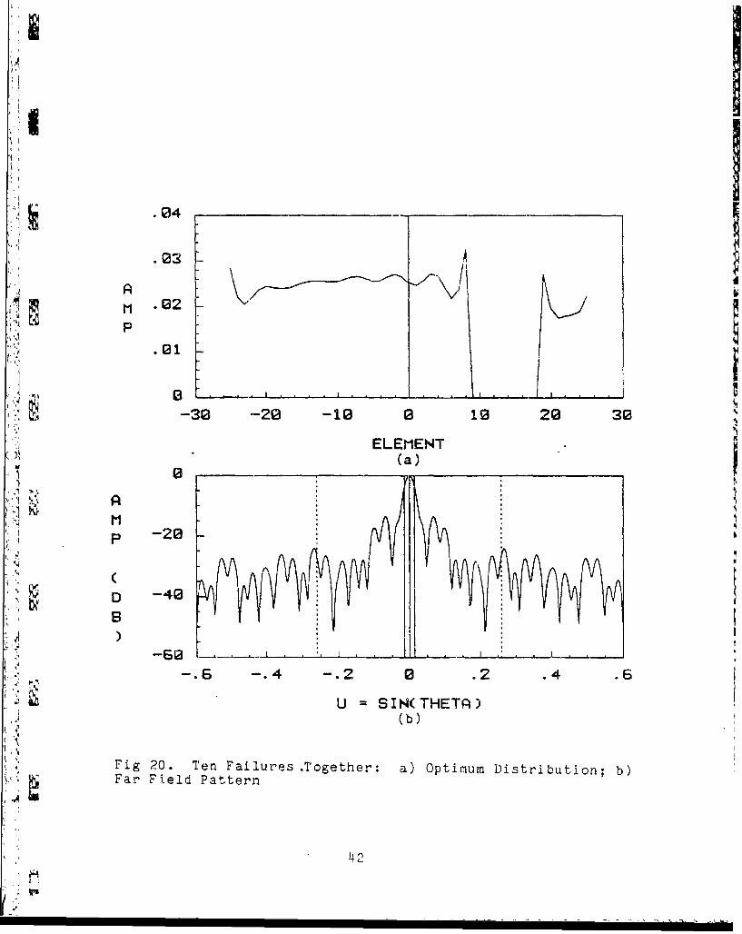
420. Ten Failures Together: a) Optimum Distribution;b) Far Field Pattern . . . . . 6 . . . . . . . . . 42

21. Correspondence of Far Field Pattern Nullsand z-plot Zeros . .... . .. . ....... 45

22. Zero Travel Due to Amplitude Perturbationsof Selected Elements of an 11 Element Array:a) Even (Elements -3, 3); b) Odd (-3, 3);c) Single (4) . . . . . . . . . . . . . . . . . . 48

23. Zero Travel Due to Phase Perturbations of Selected1Elements of an 11 Element Array: a) Single (-5);b) Single (-1); c) Single (1); d) Even (-3,3);e) Odd (-3,3) . . . . . . . . . . . ......... 50

24. Zero Travel Due to Even Amplitude Perturbationsof Elements (-3, 3) of an 11

•.Element Array with a Failure .. .. .. .. . .. 53

25. Gradient Search - Steepest DescentOptimization Method.. . . . . . . . . 56

26. Optimum Amplitude Distribution for Filled Array(Gradient Search Method) ............... 58

27. Far Field Pattern of: a) Optimum Distribution vs

b) Uniform Distribution .......... ............ . 59

28. One Failure Near End: a) Optimum Distribution;b) Far Field Pattern . . . . . . . . ....... 60

"[ 29. One Failure Center: a) Optimum Distribution;b) Far Field Pattern ......... . . . . . 61

30. Two Failures Separated: a) Optimum Distribution;b) Far Field Pattern ......... ............... 62

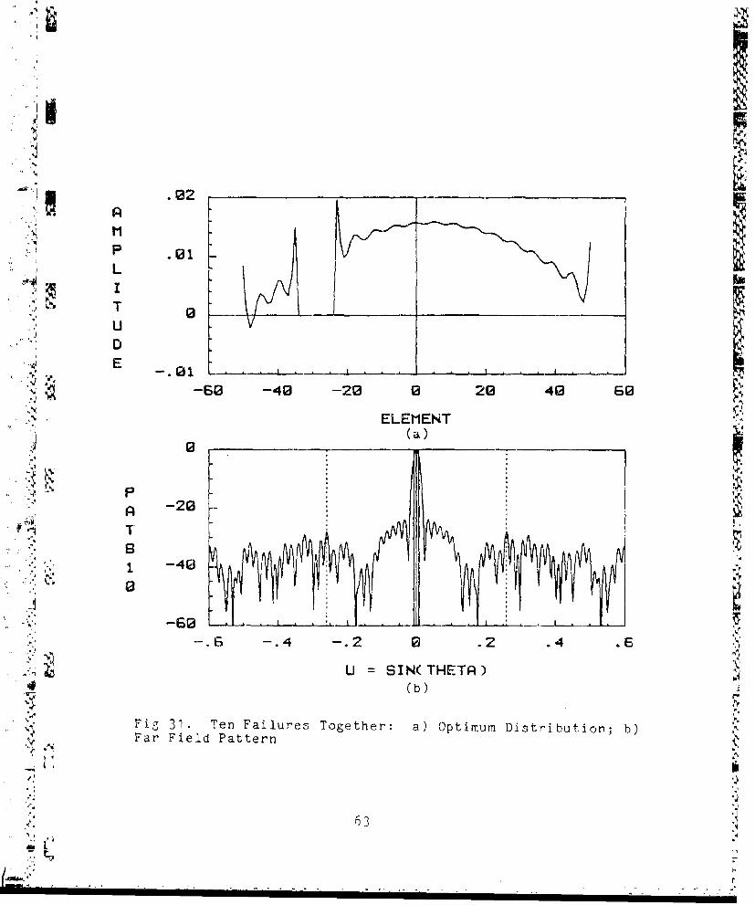
U 31. Ten Failures Together: a) Optimum Distribution;b) Far Field Pattern ............. ............... 63

32. Amplitude Distribution- a) Before andb) After Optimization ... ... 67

vii

•-I'

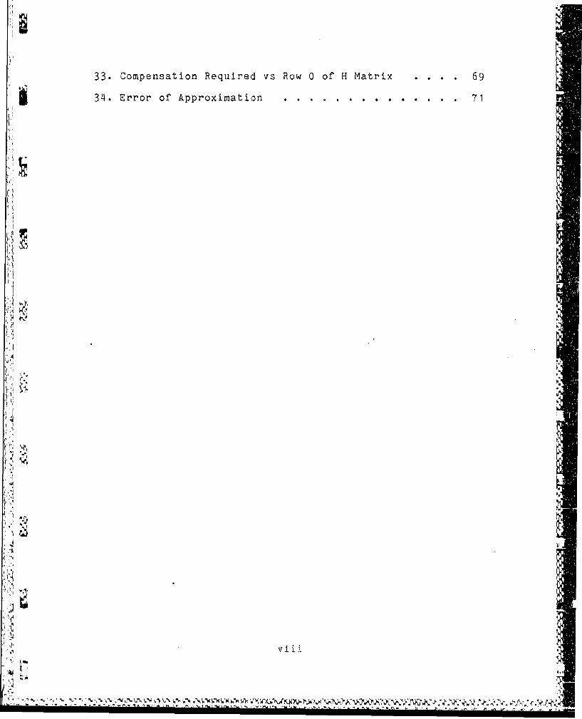
33. Compensation Required vs Row 0 of H Matrix .... 69

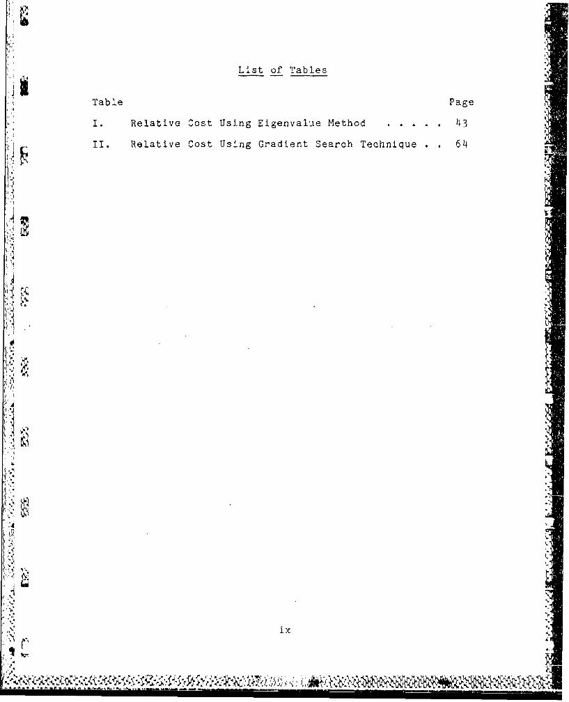
34. Error of Approximation ................ ..... ... 71

'aVil

m.I

*',.,

~ 'SW ,.b~lLt * A A~ -

LIst of Tables

Table Page

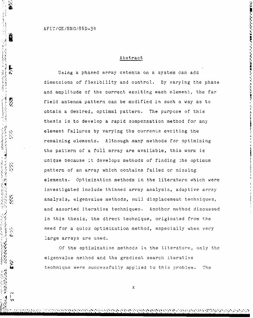
I. Relative Cost Using Eigenvalue Method ..... 43

II. Relative Cost Using Gradient Search Technique . . 64

iI L••

{'i

:4

ix

AFIT/GE/ENG/86D-34

Abstract

Using a phased array antenna on a system can add

dimensions of flexibility and control.. By varying the phase

"and amplitude of the current exciting each element, the far

field antenna pattern can be modified in such a way as to

obtain a desired, optimal pattern. The purpose of this

thesis is to develop a rapid compensation method for anyA

element failures by varying the currents exciting the

remaining elements. Altnough many methods for optimizing

the pattern of a full array are available, this work is

unique because it develops methods of finding The optimum

pattern of an array which contains failed or missing

elements. Optimization methods in the literature which were

investigated include thinned array analysis, adaptive array

analysis, eigenvalue methods, null displacement techniques,

and assorted iterative techniques. Another method discussed

in this thesis, the direct technique, originated from the

need for a quick optimization method, especially when very

large arrays are used.

Of the optimization methods in the literature, only the

eigenvalue method and the gradient search iterative

technique were successfully applied to this problem. The

x

0ý VýV)

direct method, a spin off from the eigenvalue method and the

gradient search technique, has been shown to be relatively

quick and accurate.

Recommendations for future study include the functional

(A •derivation describing the direct optimization method and

.4 including more practical aspects of phased arrays in the

propagation model.

W A

.Ix ix

.iI.

i '' . . . . . -

OPTIMIZATION OF THE ANTENNA PATTERN OF

A PHASED ARRAY WITH FAILED ELEMENTS

I. INTRODUCTION

Electrically steered phased array antennas are being

used for applications requiring a feasible, lightweight,

high gain antenna. The phased array antenna can scan its

main beam, reduce its sidelobes and improve its signal to

noise ratio by varying the amplitude and phase of the

rtn •current exciting each of the array's elements. These

capabilities make the phased array antenna ideal for use on

_J aircraft, ships, ground sites, and even satellites. A

phased array on a satellite however, has an unique problem

associated with it. Once the satellite is space-borne, the

phased array antenna is not maintainable. If for some

reason an element of the phased array no longer performs its

designed function, the antenna's far field pattern generally

degrades, i.e., the gain of the antenna decreases, the width

of the main beam widens, and the power of the peak sidelobes

increases. These degradations affect the ability of the.

phased array antenna to perform its task, which directly

affects the usefulness of the dependent system. This study

develops a rapid compensation method for any element

failure.. (or optimizes the far field pattern of an antenna

W 14 C

with failed elements), thereby extending the effective

usefulness of the phased array antenna and its dependent

system.

Background

Designing a phased array antenna for an optimum pattern

is an old problem. Techniques from thinne array analysis

[11,17,18], adaptive array analysis [1,3,18:253-259],

eigenvalue methods [2,15,16], null displacement analysis

[4,7], and assorted Iterative techniques [I0,13,14] have

been developed and used to design phased array antennas with

patterns optimized according to some desired criteria. The

variables for the design of these arrays include the

position of each element and the amplitude and phase of the

current exciting each element.

Optimizing the pattern of a phased array antenna with

L failed elements is a different problem. The study at hand

takes an existing phased array antenna (possibly designed

using one of the aforementioned techniques) which contains

failed elements and compensates for the failures

(re-optimizes) by varying the amplitude and phase of the

current exciting each of the working elements. The position

of each element is not a variable in this case, however the

solution does depend on the position of the failed element.

"2; •Assumptions

The problem can be further defined by stating the

"2

-• .". -

assumptions made:

3A. The antenna is erected in a perfect environment,with no other bodies to distort the pattern or causemultipath distortions and no other forces, such ascosmic rays, to distort the current on the elements.

B. Pattern degradation will be caused by failedelements only. The elements will fail completely -there will not be any stuc': phase shifters orpartially working amplifiers.

C. When the elements fail, the mutual coupling will beas if the element never existed (i.e. matched loadvs. parasitic load).

D. The elements will fall in clusters (due to spacedebris crashing into the array), rows (due to powersupply or computer falure), or randomly (due tolong-term individual element failures).

E. The exact position of the failed element is known.This assumption undoubtably pushes the limits ofpracticality, however, work is being done to makethis assumption more realistic [6].

F. The phased array will be mounted on a satellitewhich will be at an altitude which requires a -0.26 radians (+/- 1 5 0) scan to cover the area ofinterest. The area of interest will be called thefield of view (FOV). This assumption will ease therequirement of controlling all the sidelobes andalso allow an interelement spacing of 0.7 of thewavelength, thereby reducing the effects of mutualcoupling.

G. Although the work done should be extendable to aplanar array, this thesis applies the theories tolinear arrays only.

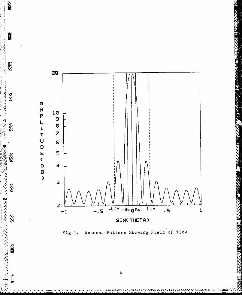
H. The pattern is defined to be optimizeG if theaverage power in the sidelobes of interest (withinthe FOV) is minimized and the power in the mainlobeis maximized (Fig 1).

Approach

Once the problem is defined, the steps to solving this

problem are first to search the literature for work which

Sl3

• •.

(

22 ----

P 20

.5

iA

10-P

L

TUDE s

D 4s), 3

-1 -Lim -Bw Bw L im

SIN( THETA)

Fig 1. Antenna Pattern Showing Field of View

.44 III

may be applicable to the problem, then to modify and apply

the work to the problem and finally to determine whether or

not the results are satisfactory.

Literature Search. Work which has been done and can be

related to this study was found through database searches

(DTIC, Analog), related indicies (Engineering Index, Science

Citation Index), prominent journals (IEEE Antennas and

Propagation), telephone conversations with experienced

experts and meetings.

Apply Knowledge. The knowledge gained from the current

literature was modified and applied to the subject problem.

To begin with, the array was described as a simple linear

array. If the technique under question can be applied to

the linear array, the technique could then be modif.ied and

applied to a planar array. Much of the analysis was done on

a VAX 11/780 using the MArRIXx software package and other

41 ADA software packages writter, specifically for this study.

Survey Results. The results were analyzed to determine

which technique best satisfied the objectives of the study.

Order of Presentation

This thesis is not presented in the traditional way.

It does contain an introductory section, a developing

section, and a concluding section, but the developing

section is different from the usual. A normal developing

section of a theoretical thesis has a chapter on existing

5

- R

i

theory, a chapter on new theory, and a chapter on

application. Because the problem of optimizing the antenna

pattern of a phased array with failed elements was attacked

by surveying several theories, the developing section of

this thesis consists of one chapter divided by the theories,

yet each theory is further divided by a description,

application, and results subsection.

p66

.............

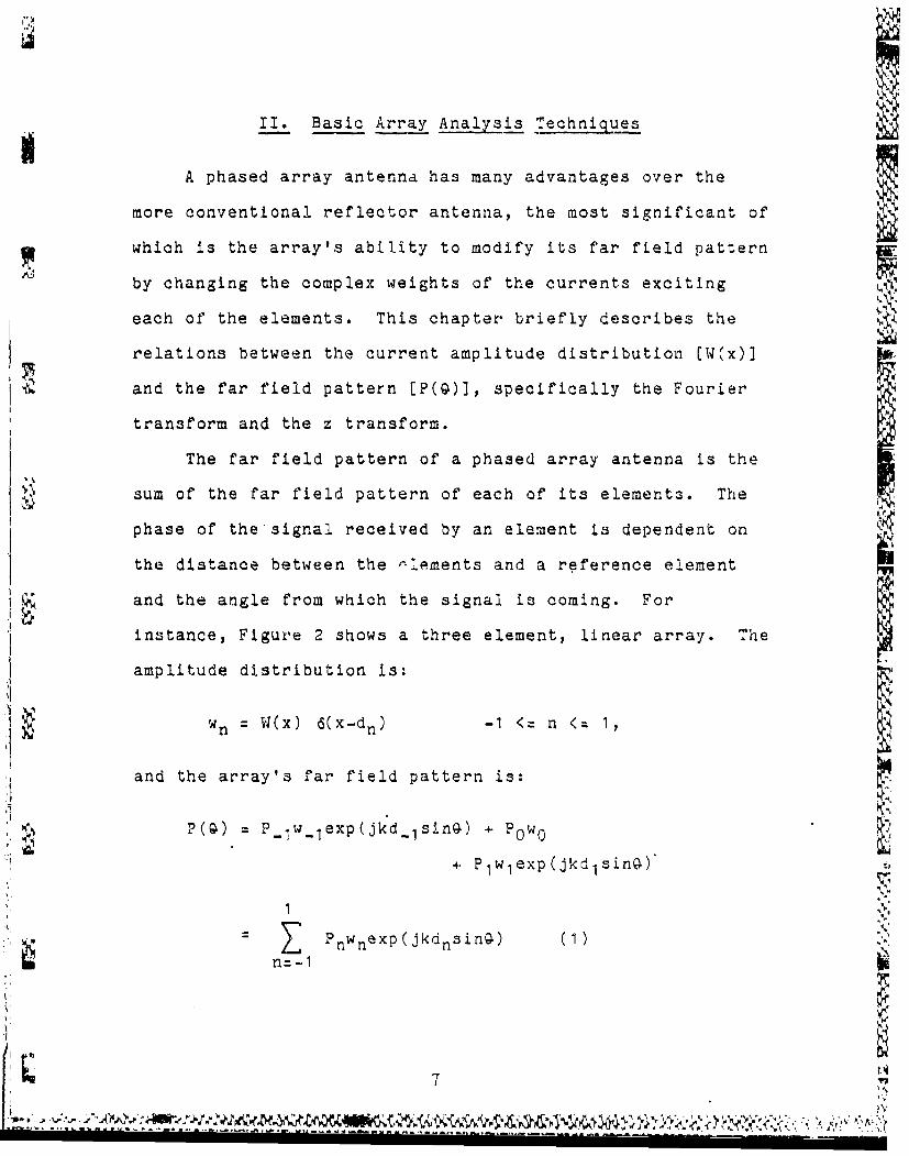
II. Basic Array Analysis Techniques

A phased array antenna has many advantages over the

more conventional reflector antenna, the most significant of

which is the array's ability to modify its far field pattern

by changing the complex weights of the currents exciting

each of the elements. This chapter briefly describes the

relations between the current amplitude distribution [W(x)]

and the far field pattern [P(g)], specifically the Fourier I

transform and the z transform.

The far field pattern of a phased array antenna is the

sum of the far field pattern of each of its elements. The

phase of the'signal received by an element is dependent on

the distance between the (lements and a reference element

• and the angle from which the signal is coming. For

instance, Figure 2 shows a three element, linear array. The

amplitude distribution is:

S= W(x) (x-dn) -1 <= n < 1,

and the array's far field pattern is:

"P(Q) = P 1w lexp(jkd 1 sinQ) + PoWo

.+ P 1Wlexp(jkdlsinQ)'

n:-1 1wexp(jkdnsing) (I)

4.

7 r

- -~•~'*J A~V~ ~~Y~~K \ %

-2 -i

° °1

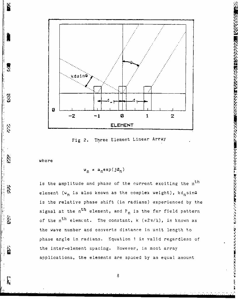
Fig 2. Three Element Linear Array

Wn anexp(jon)

is the amplitude and phase of the current exciting the nth

element (wn is also known as the complex weight), kdnsing

signal at the nth element, and P is the far field pattern

of the nth elemcnt. The constant, k (=21T/X), is known as

the wave number and converts distance in unit length to

phase angle in radians. Equation 1 is valid regardless of

the inter-element spacing. However, in most array

applications, the element~s are spaced by an equal. amount

8'

S(dn znd) - cneating a periodic array. The remainder of

this chapter will be concerned with periodic arrays with

isotropic radiators (Pn 1) as elements.

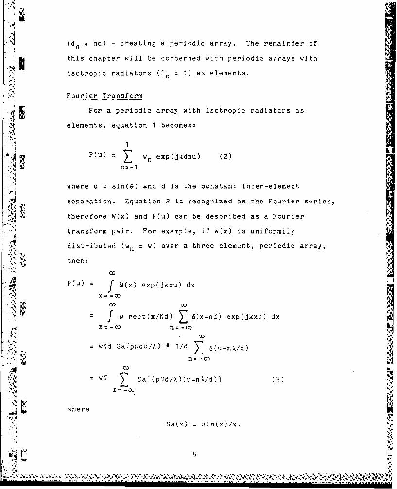
Fourier Transform

For a periodic array with isotropic radiators as

elements, equation 1 becomes:

1P(u) wn exp(jkdnu) (2)

n=-1

where u sin(g) and d is the constant inter-element

separation. Equation 2 is recognized as the Fourier series,

therefore W(x) and P(u) can be described as a Fourier

transform pair. For example, if W(x) is uniformily

distributed (wn = w) over a three element, periodic array,

"then:

P(u) f W(x) exp(jkxu) dx

X - 0

00 Co

", f w reot(x/Jd) (x-nd) exp(jkxu) dxS•X= -CD M= -r

ico

"wNd Sa(pNdu/,X) 1/d 6(u-mk/d)

wN Sa[ (pNd/X)(u-nX/d)] (3)

S• where

Sa(x) : sin(x)/x.

" " -A•

5

4

F 30U

RE

AR

• -1

-4 -3 -2 -1 0 1 2 3 4,.s

U

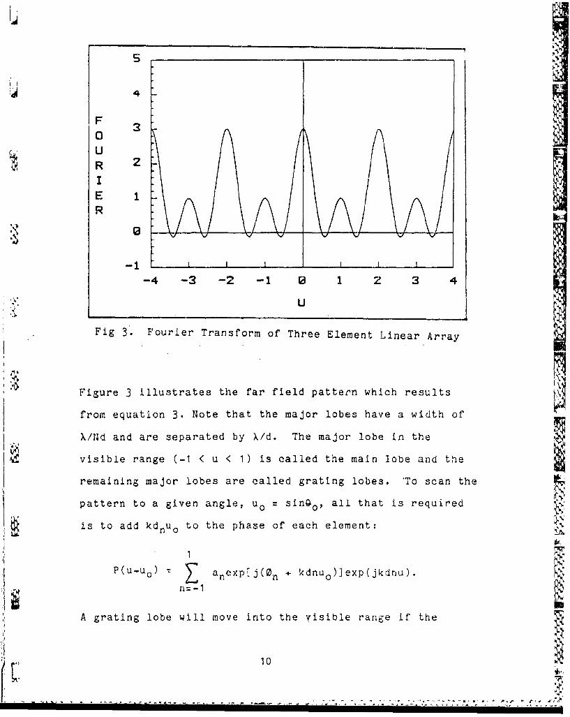
Fig 3. Fourier Transform of Three Element Linear Array

Figure 3 illustrates the far field pattern which results

from equation 3. Note that the major lobes have a width of

X/Nd and are separated by X/d. The major lobe in the

visible range (-1 < u < 1) is called the main lobe and the

remaining major lobes are called grating lobes. 'To scan the

pattern to a given angle, uo = singo, all that is required

is to add kd u to the phase of each element:no0

P(u-u anexp[J(n + kdnuo)]exp(jkdnu).S~n:-1

A grating lobe will move into the visible range if the

10S.. ......... . .. ... . ..... ... .... . ... . .... .. .. .• ,-.-, 7 ', , " ,. •" "_.•,-..:,--:y ", ",:: ":• .'I .7-

inter-element separation is greater than one wavelength or

greater than one-half wavelength with a scan of uo -I.

Z Transform

The periodic array can also be analyzed with the z

tran-form. Equation 2 can be written as:1

P(u) Z wn exp(jkdu)n

or letting

z exp(jkdu),

P(z) w Wzn (4) ¢!n:-

n=-l

2

7 (z-z.)%• m= I

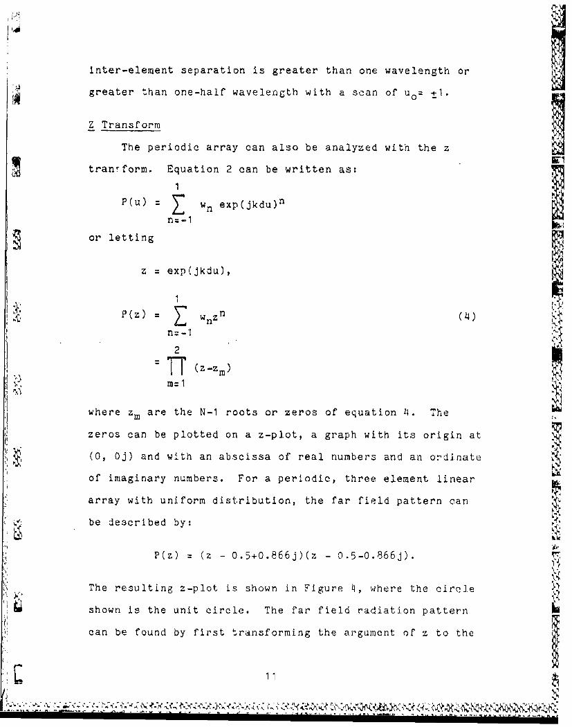
where z are the N-I roots or zeros of equation 14. The

zeros can be plotted on a z-plot, a graph with its origin at

(0, Oj) and with an abscissa of real numbers and an ordinate

of imaginary numbers. For a periodic, three element linear

array with uniform distribution, the far field pattern can

be described by:

P(z) : (z -0.5+0.866j)(z -0.5-0.866j).

The resulting z-plot is shown in Figure 4, where the circle

shown is the unit circle. The far field radiation pattern

can be found by first transforming the argument of z to the

1.5

kgIpz

6S

REL(ZE=1R u=O

Sax:

• :•, REAL( ZEROS )

Si lFi g 4. Z-plot of Three Element Linear Array

/• u axis :

u arg(z)/kd,

and then by calculating the magnitude of the normalized

radiation pattern as the product of the distance from the

point on the unit circle corresponding to arg(z) to each

root, normalized by the value of the product of the

distances from the point corresponding to arg(O) to each

root:

:" :Z-ZI! :z-z2)SI~P(z)l

12

K' i,

The visible range is -kd < arg(z) < kd. if the pattern is

scanned, z is defined as:

z = exp[jkd(u-uo)].

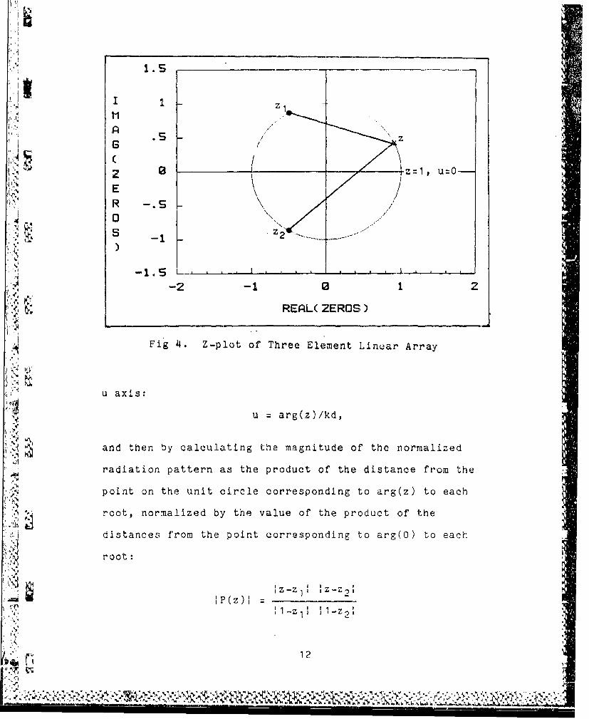
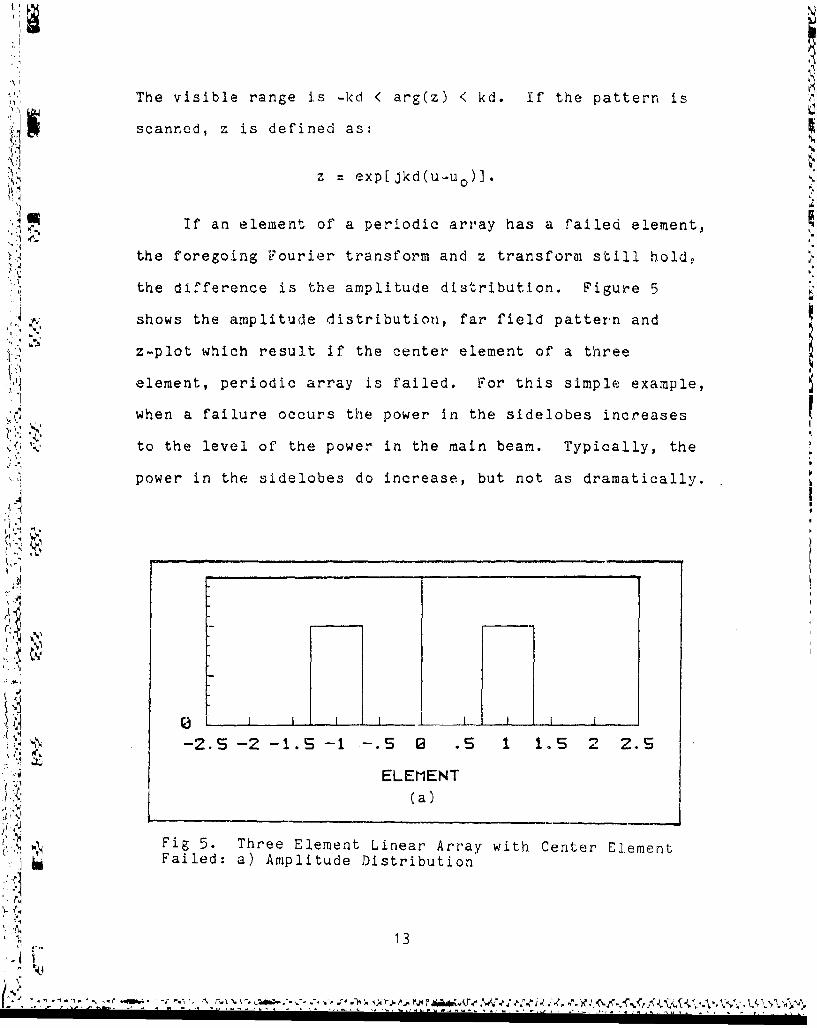
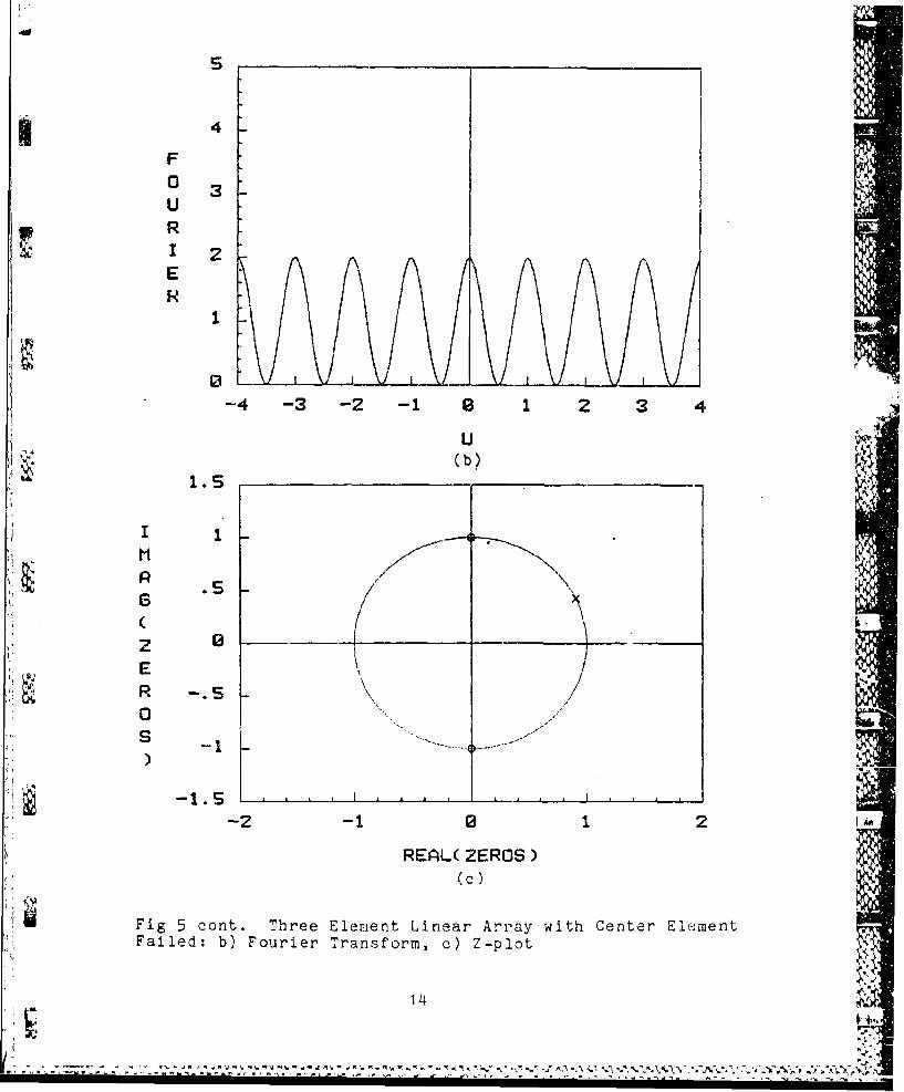
If an element of a periodic array has a failed element,

the foregoing Fourier transform and z transform still hold,

the difference is the amplitude distribution. Figure 5

shows the amplitude distribution, far field pattern and

z-plot which result if the center element of a three

element, periodic array is failed. For this simple example,

when a failure occurs the power in the sidelobes increases

to the level of the power in the main beam. Typically, the

power in the sidelobes do increase, but not as dramatically.

•'t - 1 S - - 0 S 1 1 2 Z.S

'i2.S • •'-•- ' -1 -' i " [•' •' z- "• ELEMENT

(a)

Fig 5. Three Element Linear Array with Center ElementI iFailed: a) Amplitude Distribution

13

-Mim

1 4

F03U

. I 2ER

-4 -3 -2 -1 0 2 :3 4.

U

F: 1.5

( 1,m

4 R -. S0 ...

-2 -1 2 1 2

REAL( ZEROS)(a)

Fig 5 cont. Three Element Linear Array with Center ElenmentFailed: b) Fourier Transform, c) Z-plot

14

4.1 %1 .°

III. Optimization Techniques

This section describes, in a more or less chronological

order, the work analyzed and applied in order to complete

this study. The theory behind each technique is first

described in general, a;iý then modified and applied to an

array with failed elanets, and finally tne results of

applying the theory are stated.

Y Thinned Array Analysis

.1 A filled array is a periodic array which has its

elements located at all integral oositions of a given

inter-element separation over the entire nperture. Thinned

array anilysis is a method of strategically removing and

repositioning elements of a filled array such that the far

field pattern remains satisfactory. The work done in this

. area was investigated because an array with failed elements-j

can be viewed as an accidentally thinned array.

Description. Thinned arrays are usually created usingeither a deterministic, statistic, or random method. One

way to build a deterministically thinned array is to choose

a continuous current distribution function which corresponds

to the desired far field pattern and then sample the

function with the given number o elements in such a way as

to minimize the quantization error [17:212]. For small

numbers of elements and linear arrays, this is a fairly

simple process. For large number of elements or planar

15

1. -

arrays, it is more common to use a statistical method.

Furthermore, it has been shown that the arrays designed

using deterministic methods exhibit average properties

similar in character and level to arrays designed using

statistical methods [18:132]. A statistically thinned

array, like the deterministically thinned array, is also

designed by first choosing the appropriate current

distribution function, however, the elements are then

positioned according to the probabilities of the normalized

-'urrent distribution function [17:219]. For instance, the

peak of the amplitude distribution, which is usually in the

center of the aperture, would have a probability of one.

Therefore, an element would be placed in the center of the

__ array. The probability that an element would be placed on

O • the edge of the tapered distribution would be smaller.

Statistically thinned arrays are sometimes equated to

randomly thinned arrays [18:140]. However, for this paper,

the difference mupt be distinct. A randomly thinned ari'ay

is an antenna created by randomly removing elements, either

intentionally or accidentally (see assumptions), from a

filled array.

It is difficult to quantify the effects that thinning

an array has on the pattern for the deterministic method.

The other methods can be described with statistics,

therefore the average pattern can be de:ocribed. Thinning an

o0 iarray decreases the peak power of the main beam (assuming

"• ~16,r

additional current is not added to the remaining elements)

and increases the floor of the sidelobes. In other words,

the average power pattern can be modeled as:

IP(u)I2 IP 0 (u), 2 (1-1/N) + 1/N

where P0 (u) is the desired array factor and N is the number

of elements in the statistically thinned array. The first

term on the right hand side of the equation shows the

average reduction in power and the.second term shows the

average increase in the floor of the sidelobes. Further

analysis shows that the probability density function of the

power of the sidelobes reduces to a Rayleigh distribution:!',

p[NjP(u)1] = 2 :P(u)? exp(-N jP(u): 2 )

where NfP(u)l is the unnormalized amplitude of the complex

radiation pattern of an N element array.

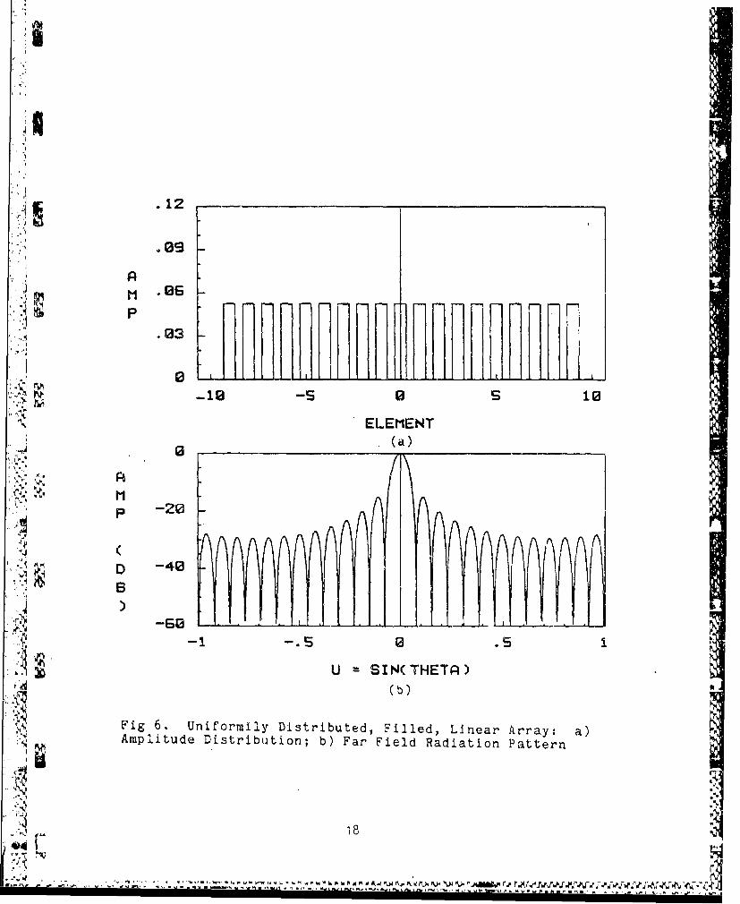
Application. To illustrate the effects of thinning an

array, three patterns are produced from three arrays

designed with different amplitude and spatial tapers. For

comparison purposes, all the patterns are normalized. The

first array (Fig 6) is a uniformly distributed, filled,

I linear array with 19 elements. The second array (Fig 7) is

similar to the first array except that the amplitude

disti ibution is triangular. The final array (Fig 8) is a

thinned array made of 15 equal amplitude elements spatially

tapered such that each element corresponds to equal areas

17

.12 -

.09

iA

M .0S

I,

-1 -5 S 10

ELEMENT

.. (.) ,..

MP -20

0D -40

B

,. -6W

U = SIN(THETA)(b)

Fig 6. Uniformily Distributed, Filled, Linear Array: a)Amplitude Distribution; b) Far Field Radiation Pattern

54.*k P r.- .. 4 V .l.,J4 4 14. h 'p•trn n 4 * 4 .-l4

AA

M .06P

.03

ELEMENT"0 _ _ _ _(a)

-20-

-40

U = SIN(THETA)

(b)Fig 7. Triangular Amplitude Taper Distribution, Filled,Linear Array: a) Amplitude Distribution, b) Far FieldRadiation Pattern

19-. •.

(m ; ..,

.jJ .12 -

.1. 9A

M .26 fPH

.3ILI

" -12 -5 2 s 12

ELEMENT(a)

P

I . '~

D -40"B"--

-1 -. 5 2 .5

U = SIN(THETA)

(b)

Fig 8. Triangular Spatial Taper Distribution, Thinned,Linear Array: a) Amplitude Distribution, b) Far Field N]Radiation Pattern

20

S... .' .. .... *, * "- ~ " -, ",, *" . W ". '. 2,,' ", , ,". ". -" , 'A " .A , ' - .,• V •. ..- , V- .. 7'"-- V, , ''• ,•' ",",.- ." )7'•'•. w .," , -Z

under the triangular distribution. Note that there is a

practical limit to the positions the elements can be

placed. For instance, mutual coupling affects and actual

element size dictate the minimum separation.

Results. At first, it was hoped that a pattern similar

to Figure 8, a pattern with low sidelobes in the FOV, could

be obtained using thinned array analysis. However, thinned

array analysis is used to design phased array antennas and

could not be adapted to determine the necessary compensation

for any element failures. Thinned array analysis can be

used to determine where elements should be placed in order

to obtain a desired pattern, but in the given problem, the

position of the elements failed is not a variable.

The statistics developed to analyze the patterns of

thinned arrays are useful in determining what the pattern

would look like after element failures occur, but the goal

of this study is to improve the pattern.

Adaptive Arra• Analysis

Adaptive array anaylsis [18:253-269] encompasses the

methods of actively optimizing the pattern of a phased array

antenna based on information processed from the received

signal. Usually, in this case, a pattern will be optimized

if the signal to no.se ratio is maximized. Therefore,

adaptive arrays aru specially concerned with nulling out

jammers and other sources of unwanted signals in the

21

4'

environment. Adaptive arrays also have the capability to

compensate for normal variations In an element's position

and complex current weight, which is the reason for

investigating this technique.

Description. Two of the most notable methods for

building adaptive arrays are the nulling tree method and the

least mean square error (LMS) method.

An adaptive array with nulling tree hardware (Fig 9)

has the ability to null out any type of signal, if the

direction of the interference is known. To create and scan

a null, the control hardware modifies the complex weights of

"one row of the nulling hardware. All the weights in the row

are the same and each row creates only one null. The

complex radiation pattern (P(u)) is the product of the

original pattern (Po(u)) and the patterns created by the

nulling hardware (P 1 (u), ... , PK(u)) or

P(u) : (Po(U)) (PI(u)) (PK(u))

A where

N

Po(U) Z wmexp(jkdmu),

m=1

PK(U) exp(jkdu) - exp(jkduK),

N = the number of elements,

K = the number of rows of nulling hardware,

Sr 22

. . . . . . . . . . . . . .. . . .

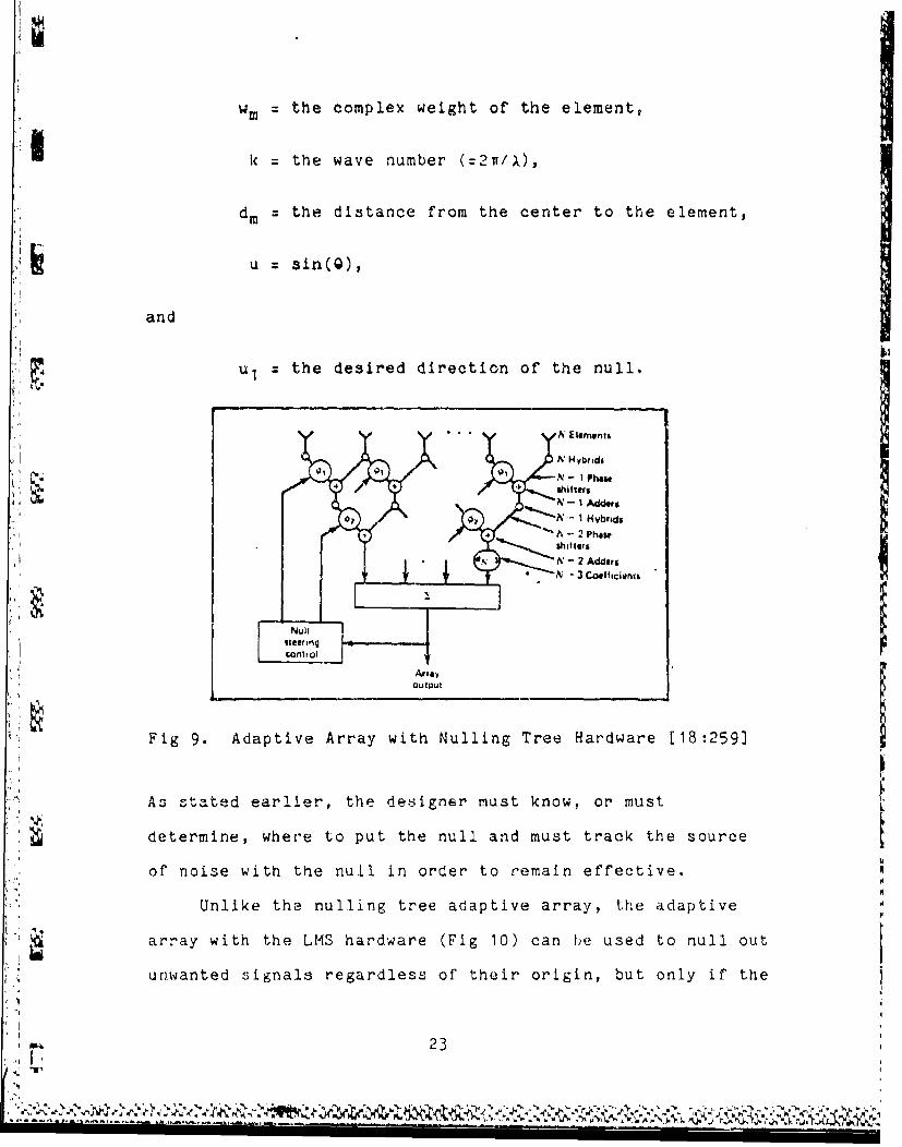
wm = the complex weight of the element,

kI = the wave number (:2x/X),

dm = the distance from the center to the element,

u sin(Q),

and

U1 -the desired direction of the null.

A; l-mentici

,K -- -I Aidds1 Hvbids

, • /• -"2 Phase•$,hilters"X' - 2 Add.es

S] J . Ai 3 Coefficients

ArrayOUICput

Fig 9. Adaptive Array with Nulling Tree Hardware [18:259]

A3 staVted earlieri the designer must know, or must

"determine, where to put the null and must track the source

of noise with the null in order to remain effective.

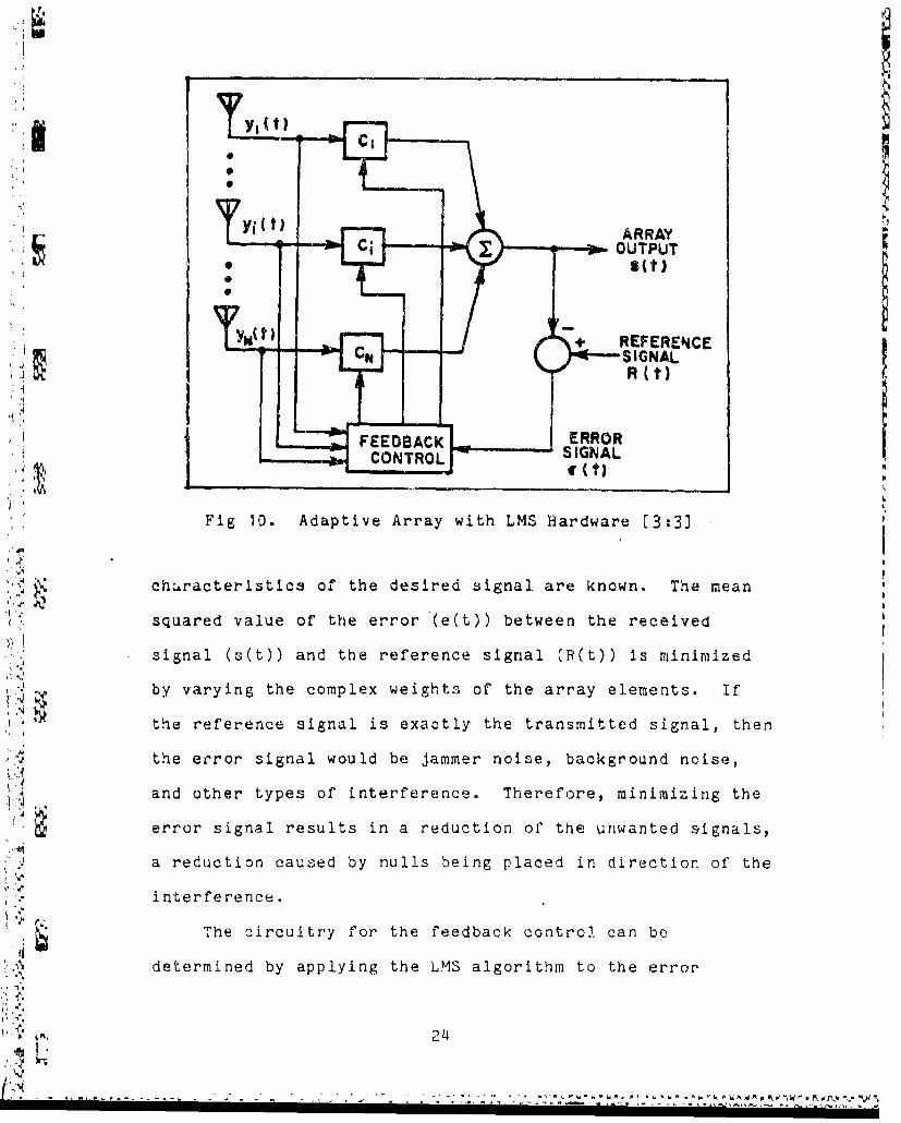
Unlike the nulling tree adaptive array, the adaptive

A • array with the LMS hardware (Fig 10) can be used to null out

unwanted signals regardless of their origin, but only if the

23It.

;Nj

cif yi t)} 1 ARRAY" • -4 i i€ OUTPUT

Fig10.Adaptive Array with LMS Hadwr [3:3]

1A characteristics of the desired signal are known. The mean

squared value of' the error (e(t)) between the received

signal (s(t)) and the reference signal (B(t)) is minimized

by varying the complex weights of the array elements. if

the reference signal is exactly the transmitted signal, then

the error signal would be jammner noise, background noise,

and other types of interference. Therefore, minim~izing the

error signal results in a reduction of the unwanted aignals,

a reduction caused by nulls being placed in direction of the

interference.

The c-ircuitry for the feedback controJ. can be

determined by applying the LMS algorithm to the error

124

W jd A 2%6

signal. The error signal is:

i ~ e(t) R(t) -s(t) .<

N

= R(t) - wiyi(t)

wh. "e w, is the complex weight of each element and yi(t) is

the received signal. The time-average value of e 2 (t) is:

e2(t) r2(t) -2 yjtR)

N N

S+ i1 wiwjyi(t)yj(t)

i=I J=1

To minimize the mean square error, the complex weights can

be varted according to the LMS algorithm:

, ~dwi/dt = -k d[e 2 (t)]/dw 4

or

dwi/dt = 2kyi(t)e(t) (5)

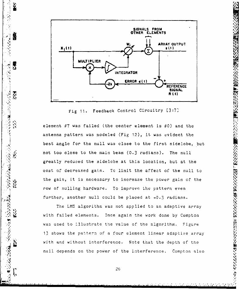
Finally, the circuit (Fig 11) is derived from integrating

equation 5:!' t

li• •wi =Wio + 2k f• Yi(t)e(t)dt

-! 0

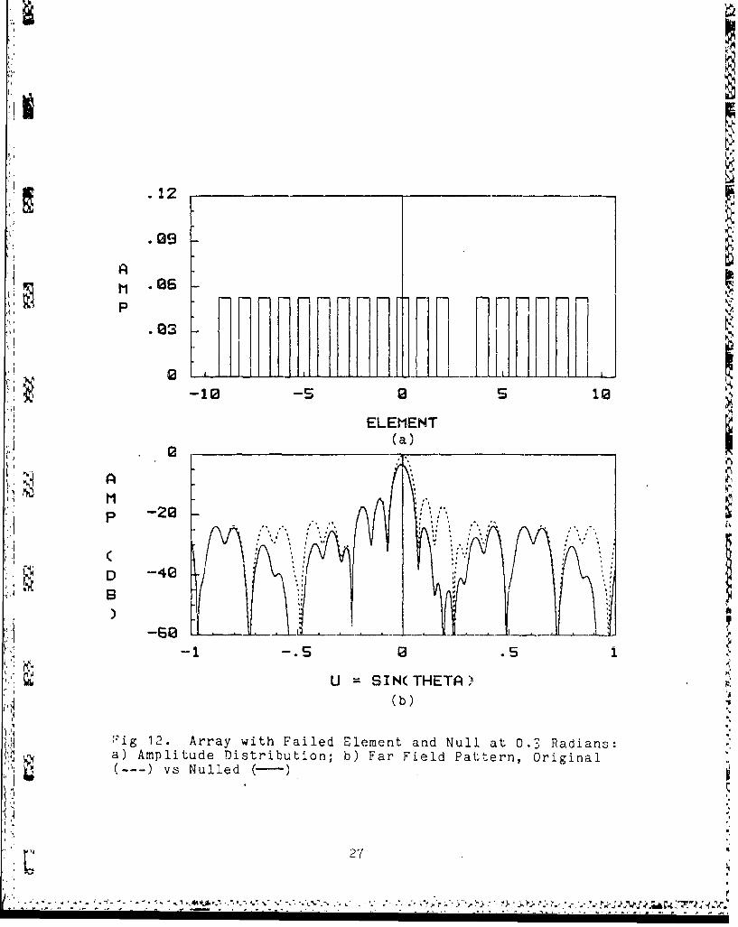
Application. A 21 element, linear, nulling tree

adaptive array was designed to determine the applicability

of this technique to an array with failed elements. After

•' • 25

I

'IISIGNALS FROM

A4 OTHER ELEMENTSF 1 Fea CW.t ARRAY OUTPUT

'" . i "

eleen,#,w aie(teenERReORlemt is +he

R R t)

1 Fig 11 Feedback Control Circuitry [3:71

:.> •.element #7 was failed (the center element is #0) and the

antenna pattern was modeled (Fig 12.), it was evident the

best angle for the null was close to the first sidelobe., but

not too close to the main beam (0.3 radians). The null

greatly reduced the sidelobe at this location, but at the

,4 cost of decreased gain. To limit the affect of the null to

the gain, it is necessary to increase the power gain of the

row of nulling hardware. To improve the pattern even

further, another null could be placed at -0.3 radians.

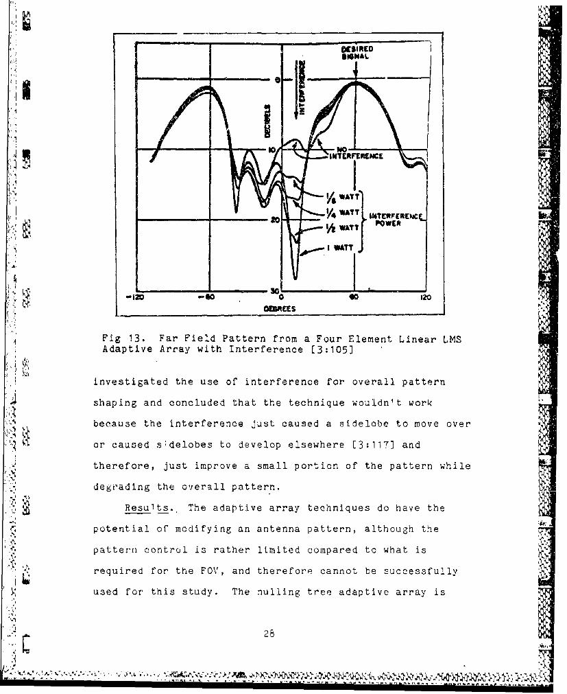
The LMS algorithm was not applied to an adaptive array

"with failed elements. Once again the work done by Comptoni-.

was used to illustrate the value of the algorithm. Figure

13 shows the pattern of a four element linear adaptive array

with and without interference. Note that the depth of the

null depends on the power of the interference. Compton also

26

UA 1210

ELEMENT

P -20

.1a3JlFlF. ] f p6-1 0

P, -20-S .

U =SIN(THETA

S(b)

'ig 12. Array with Failed Element and Null at 0.3 Radians:a) Amplitude Distribution; b) Far Field Pattern, Original

vs Nulled (-)

27

........ ... . ...... - a---------------------------- ..- -.... .-#' .# :.,7. ..-.

ISMAL

- -

_ _._ _•_Y __IA MTERFEMNCL

12 .g 0 120, O[I RL 'S p.

"Fig 13. Far Field Pattern from a Four Element Linear LMSAdaptive Array with Interference [3:105]

investigated the use of interference for overall pattern

shaping and concluded that the technique wouldn't work

because the interference just caused a sidelobe to move over

, ~ or caused s:delobes to develop elsewhere [3:117] and

therefore, just improve a small portion of the pattern while

degoading the overall patt-rn.

"A',_,Results. The adaptive array techniques do have the

potential of modifying an antenna pattern, although the

pattern control is rather limited compared to what is

"required for the FOV, and therefore cannot be successfully

used for, this study. The nulling tree adaptive array is

28*A., YA *C 28 v,

< urther unattractive because of the additional hardware

required and because apriori knowledge required of where to

place the null.

An optimization method similar to the LMS algorithm

(called the steepest descent gradient) was used in a

following section as an iterative technique. However,

reduction of interference will not be the main goal there.

Eigenvalue Methods

Eigenvalue methods are methods which, thru the marvels

of linear algebra, analytically arrive at a solution which

will maximize or minimize a given function. The advartage

-• • of using these methods is they are relatively quick to come

to a solution compared to the other techniques investigated.

Description. Two different eigenvalue methods were

tried, one by Cheng [2] and the other by Shore [15].

Cheng's eigenvalue method is based on a theorem on the

properties of a function of a matrix vector. The theorem

says that given a function:

"G = aTAa / aT*Ba

where a is an Nxl column matrix, A and B are both Hermitian,

NxN square matricies, and B is positive definite, then:

"�T'-i 1. The roots (eigenvalues) of the characteristic equationare real.

2. The minimum eigenvalue and maximum eigenvalue

represent the bounds of G:

29

1.x.4.

< G<

S3. G is maximized when:

Aa X Ba

or minimized when

Aa : IBa.

Cheng applied the theorem to maximize the gain of an array:

':•,. ~ S ( U o , o& & :(6)

.,1/I(4 ) fd s(u,Q)du

where-

" _., s ( u , g ) = p ( u ) j ,

P is the element power pattern (=I for isotropic elements),

"and the other symbols are as before. Equation 6 can be

written as:

G wT*Aw / WT*Bw

where W is a column vector whose elements are the coiiplex

4-4 weights of the current distribution and A and B are

Hermitian, square matricies with elements

Amn exp[jk(dn - dm )U]AMS30

and

Bmn Sa [k(dn - dm)]

respectively, and B is positive definite. To solve for W,

the A matrix is decomposed into

A SS(7)

where S is an 14 element vector with elements s exp(-Jkdm

u). Finally, the optimum current distribution and the

maximum gain are:

W =B-1

and

Gmax S B-1S.

Shore's eigenvalue method re.lies on Lagrangian

multipliers to find the current distribution which gives the

optimized pattern. The objective of Shore's work was to

minimize the power within a spec fied interval of the

antenna pattern with constraints on the weight perturbations

,,I required and the value of the look direction gain. The ,cost

function, which is the function to be minimized, is modeled

SIby;

G (W-Wo)T(w-wo0 ) + ulWT*cw.

The first term on the right hand side of the equation

31

minimizes the weight perturbations and is the square of the

change in the weights (W = vector of perturbed weights, W.

vector of original weights) scaled by a factor (uI) which

increases or decreases the relative importance of minimizing

the perturbations versus the minimizing the sidelobe

sector. The second term corresponds to the power within the

sidelobe sector which is to be minimized:

Uo+ewT*cw = 1/2e u2 du

f IP(u); dUO-e

where' uo and e are the center and the range of the sidelobe

sector respectively and C is a Hermitian, Toeplitz matrix

whose elements are:

Cinn exp[j(dn-dm)uo] Sa(dn-dm)e]

By taking the derivative of the cost function with respect

to the complex weight, setting it equal to zero, and solving

for W, the current distribution which corresponds to the

optimum pattern is:

W = AWo

where

A (I + uIC)' 1 .

Shore constrained the cost function not only by minimizing

the weight perturbations, but also by specifying the look

32

.......................................

direction gain. The look direction gain is defined as

g = ST*W

where S is as before except u (=uo) is the desired direction

of the main beam. The solution constrained to a given gain

is found by using the method of Lagrangian multipliers and

is:

NW A[W - ( (ST*AWo - g)/ST*AS )SJ (8)

As the relative importance of limiting the weight

perturbations increases (i.e., uI goes to 0), W converges to

0 and as the relative importance of minimizing the power in

the sidelobe sector increases (i.e., uI goes to Infinity),

W : (C-s / sT*c-s) g.

"Both Cheng's method and Shore's method result in a

straight forward equation to be solved and both can be

solved for a general array. A trivial difference between

the two methods is that Cheng is trying to maximize a

function whereas Shore is trying to minimize a function.

.Ap2plication. The function which relates to the optimum

pattern for this study was alluded to in the assumptions and

Ils:

""-Bw Bw Lim

G f !P(u): du -i 5f P(u)!2du + fPu2 d-Lim -Bw Bw

4111c

33 3.

Lim Bw

-Lim -Bw

= P(u) 2adu - (i~si)f :p(u)1 2du _

N N

SWn w m Hmn (9)

n=1 m=1

where sI is a scale factor which adjusts the relative

importance of maximizing the power in the main lobe versus

minimizing the power in the FOV, Bw is the one sided main

lobe beam width (= sin(1/(O.7N)) * 0.5), Lim is the bound of

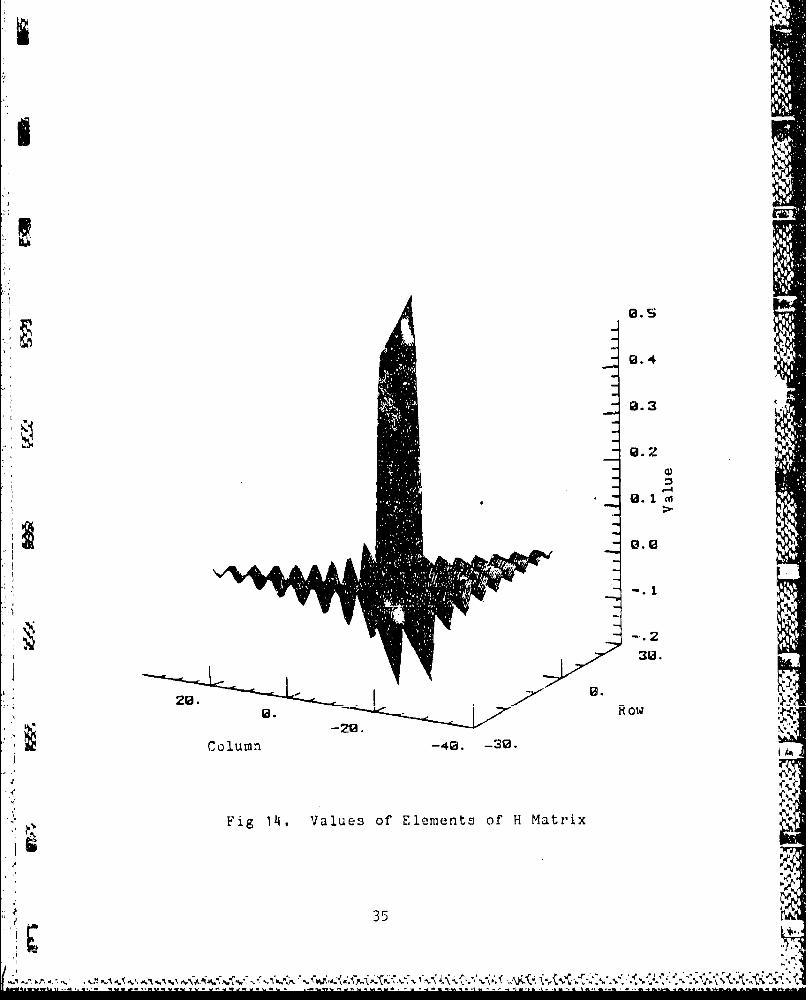
the FOV (= sin(0.26)), H is a Hermitian, Toopliz matrix (Fig

14) with elements

Hmn 2Lim Sa[k(dn-dm)Lim] - 2(1+sl)Bw Sa[k(dn-dm)Bw] (10)

and the remaining variables are as previously described.

The H matrix will replace the A matrix in Cheng's method and

the C matrix in Shore's method.

The difficulty in applying Cheng's method came with the

decomposition (eqn 7). In order for the decomposition to

work the H matrix must be separable into the product of a

"column matrix and its complex conjugate, but because the H

"matrix is the result of summing three different areas of the

far field pattern, it is not separable as Cheng's A matrix

"was separated.

Shore's method; however, can be successfully applied.

":4 Figure 15 depicts the amplitude distribution resulting from

S--. ..34

*N1

' '1i0. S

(0.4

30.z

"Q. Row

Column -40. -30.

Fig 14. Values of Elements of H Matrix

.1 35 1

ei

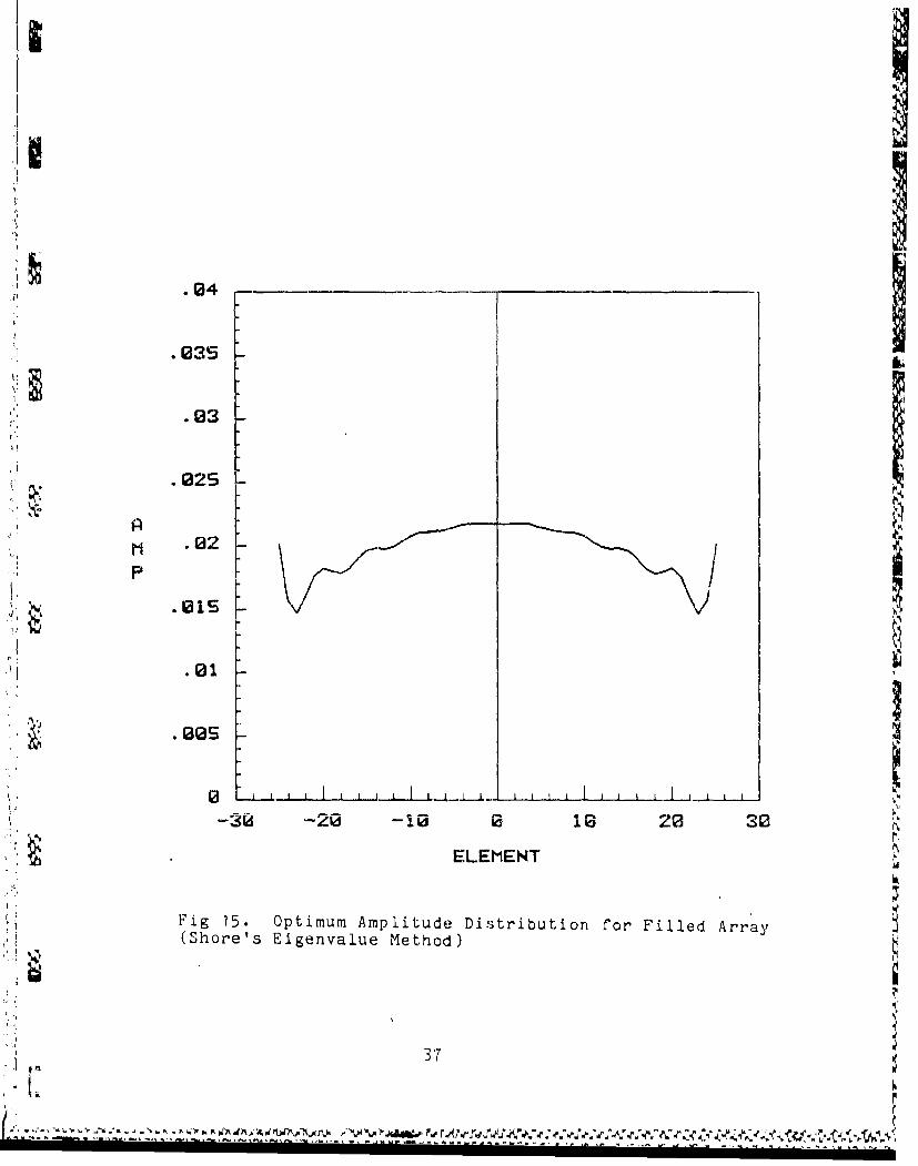
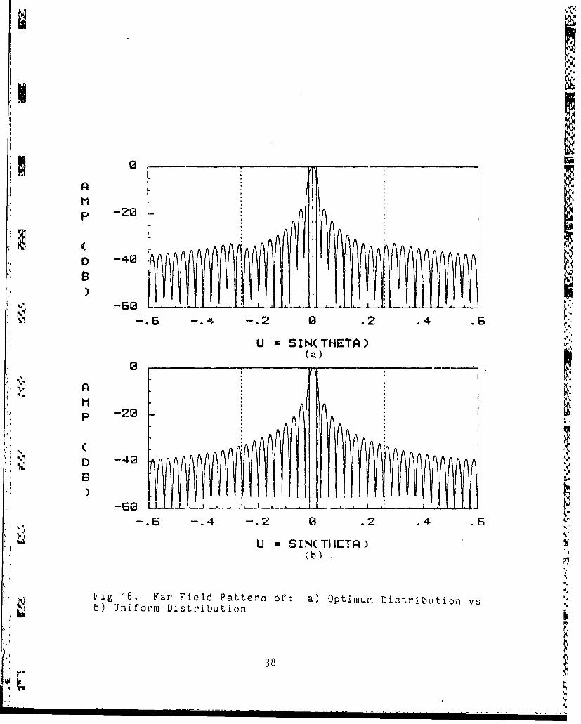
optimizing a 51 element linear array with unity scaling

factor. Figure 16 shows the resulting far field power

N pattern compared uo the pattern of an uniform distribution.

Note "hat, as a result of the tapered amplitude

distribution, the sidelobes in the FOV are reduced, but the

width of the main beam ii; increased. If an element is

failed, initially it was believed that the elements'

corresponding complex weight could be set to zero. After

"the equation was applied however, a value was assigned to

the failed element. To correct for this anomoly, the row

and column of the H matrix corresponding to the failed

element were set equal to zero. This changed the H matrix

into a singular matrix, the inverse of which is does not

exist. Finally, it was realized that the H matrix did not

require a periodic Inter-element separation. Because of

this, the row and column of the H matrix corresponding to

the failed element could simply be removed, reducing the

matri.x to an 1-I by N-i square matrix. After appropriately

reducing the orders of the remaining matricies, the mode.

(eqn 8) was reapplied. Figures 15 - 20 show the amplitude

'] distribution and the normalized antenna pattern of a 51

element linear array for five cases: a) optimum

distribution, no failures; b) optimum distribution, one

failure (near end: #21); c) optimum distr.ibution, one

failure (center: #0); d) optimum distribution, two failures

(separated: #5, #.-16); e) optimum distribution, ten failures

'~*.I'

II

.04

A' 03

.025

M

P

X1.,

K ELEMENT

Fig 15. Optimum Amplitude Distribution for Filled Array(Shore's Elgenvalue Method)

S37

SI

( - -2 1 i.(2 o•,

|i

MP -20

-40

-. 6 -. 4 -. 2 0 .2 .4 .6

U SIN(THETA)(a)

0

P -20

D0 4

-. 6 -.4 -. 2 0 .2.

U SIN(THETA) 9(b) ,

Fig i6. Far Fiel.d Pattern of: a) Optimum Distribution vgb) Uniform Distribution

38

r3...... ..

.03

M .02P

.01

0• • ---.- . . . . • • , • • , , , t . .. . _-

-30 -20 -10 0 10 29 30

ELEMENT(a)

0M

P -20

-D -40

)

-. 6 -. 4 -. 2 0 .2 .4 .6

U = SIN(THETA)(b)

Fig 17. One Failure Near End: a) Optimum Distribution; b)"Far Field Pattern

39

,ft

•1 .04 -_ _

.03

"IP_._ _ _ _ _ _

-30 -20 -10 0 10 20 30

ELEMENT(a)

M2

P -22 .,.

D -41) I

-. 6 -. 4 -. 2 0 .2 .4 .6

U = SIN(THETA) h(b)

Fig 18. One Failure Center: a) Optimum Distribution; b)Far Field Pattern

4O

.04 -

M! .02

.01

I..__.J_ __ _ .. _,_•

-30 -20 -10 0 10 20 30

ELEMENT(a)

mSp

.- 20

SD -40

-. 6 -. 4 -. 2 0 .2 .4 .6

U = SIN(THETA)(b)

"Fig 19. Two Failures Separated: a) Optimum Distribution;b) Far Field Pattern

"°14

S......... ....... . ... .. .... .. . .. .. . "- .. . ,"" 2 :- " ' . . .....

I.1

<,A

P.04

.01

-30 -20 -10 2 10 20 30

ELEMENT

., ..a

M -

P -20

D -40B

-. 6 -. 4 -. 2 0 .2 .4 .6

U = SIN(THETA)(b)

Fig 20. Ten Failures .Together: a) Optimum Distribution; b)Far Field Pattern

S42

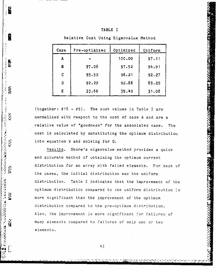
TABLE I

Relative Cost Using Eigenvalue Method

Case Pre-optimized Optimized Uniform

A 1 100.00 97.11

B 97.08 97.52 94.91

C 95.52 96.21 92.27

"D 92.22 92.88 89.29

E 33.66 35.49 31.08

S

(together: #18 - #9). The cost values in Table I are

normalized with respect to the cost of case A and are a

relative value of "goodness" for the associated case. The

cost is calculated by substituting the optimum distribution

S. '• into equation 9 and solving for G.

Results. Shore's eigenvalue method provides a quick

and accurate method of obtaining the optimum current

distribution for an array with failed elements. For each of

the cases, the initial distribution was the uniform

distribution. Table I indicates that the improvement of the

optimum distribution compared to che uniform distribution is

more significant than the improvement of the optimum

distribution compared to the pre-optimum distribution.

Also, the improvement is more significant for failures of

many elements compared to failures of only one or two

elements.

I43

Null Displacement Technique

<5 Null displacement is a method of quickly optimizing an

antenna pattern by modifying the positions of the pattern

nulls. This method is useful because the angular position

of the pattern's nulls plotted on a z-plot is the

z-transform of the current distribution. Therefore, once

the position of the pattern's nulls have been defined, the

required amplitude and phase of the current exciting each

Ii Ielement can be easily determnined by using the inverse

z-transform.

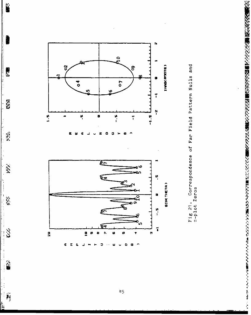
i !Description. The roots (zeros) of the z-transform of

-" •-an array factor can be moved by varying the complex weight

of the currents on each element. The zeros, if on the unit

circle of the z-plot, represent a null in the antenna

pattern. If the zero is not on the unit circle, the pattern

dips at the location of the zero, but does not null (Fig

21). Also, the closer the zeros are to each other, the

lower the peak power of the lobe between them. The nulls 4

through 7 exist twice within the visible range (-1 < u " 1,

-1.4f < arg(z) < 1.40) of the antenna pattern because of the

0.7X inter-element separation. Therefore, the cost function

(eqn 9) is minimized if the zeros corresponding to the nulls

beside the main beam were held constant and all the other

zeros were moved into the FOV. Gaushell [71 has shown that

the amplitude distribution which creates a desired pattern

can be determined by first modifing the positions of the

411

0 CL

~~~~~~0 0 I I 0 0 I 1 ^I

,I __ __

N_"0

V4V

I-,

45

). e

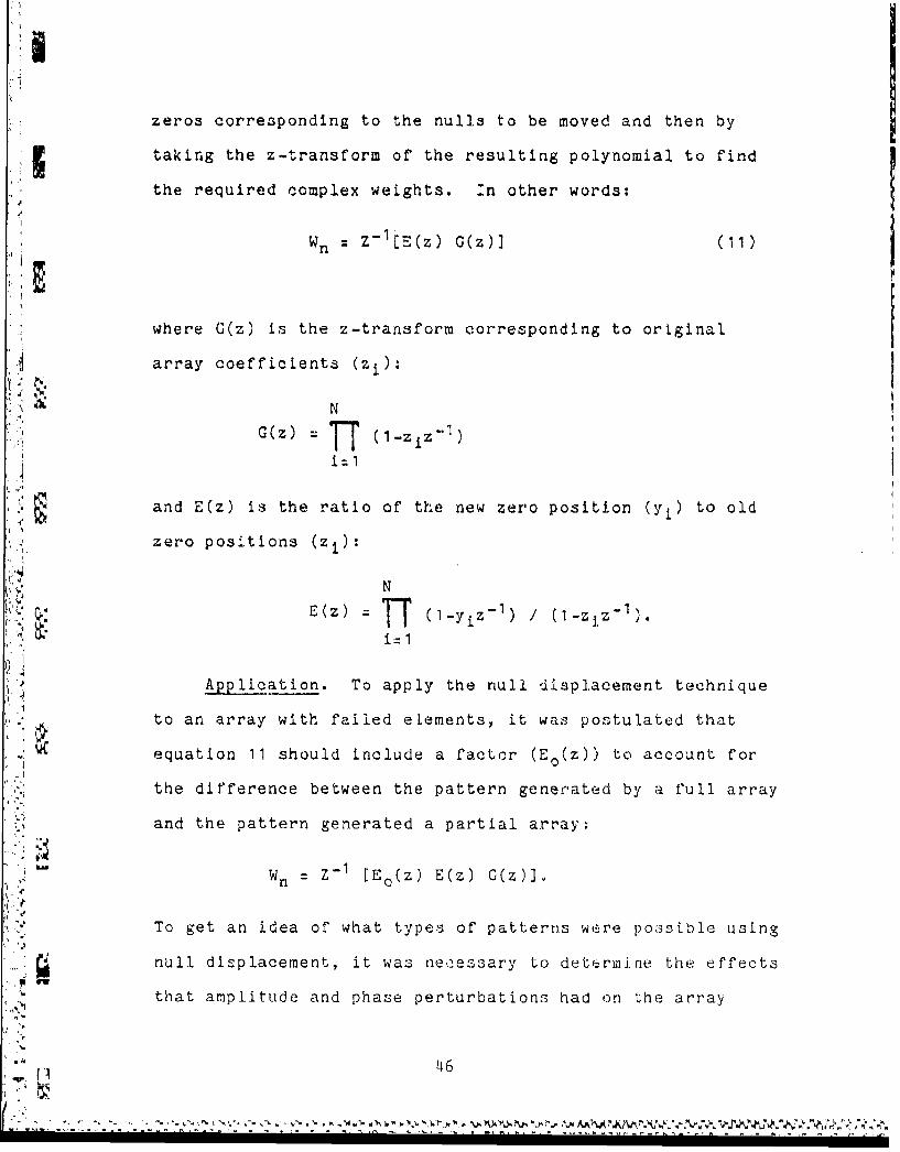
zeros corre3ponding to the nulls to be moved and then by

taking the z-transform of the resulting polynomial to find

the required complex weights. In other words:

, ~Wn Z-I[E(z) G(z)] (1

where G(z) is the z-transform corresponding to original

array coefficients (zi):

NG(z) V Z Ci.zjz-

and E(z) is the ratio of the new zero position (y1 ) to old

zero positions (zi):

NE(z) 7 (1-yiz- 1) (1-ziz- 1).

A2plication. To apply the null displacement technique

to an array with failed eLements, it was postulated that

"equation 11 should include a factor (Eo(z)) to account for

the difference between the pattern generated by a full array

. and the pattern generated a partial array;

" i- wn = Z-1 lE,(z) E(z) G(z)].

- To get an idea of what types of patterns were po,3ssible using

null displacement, it was necessary to determine the effects

that amplitude and phase perturbations had on the array

116

- - - - INA

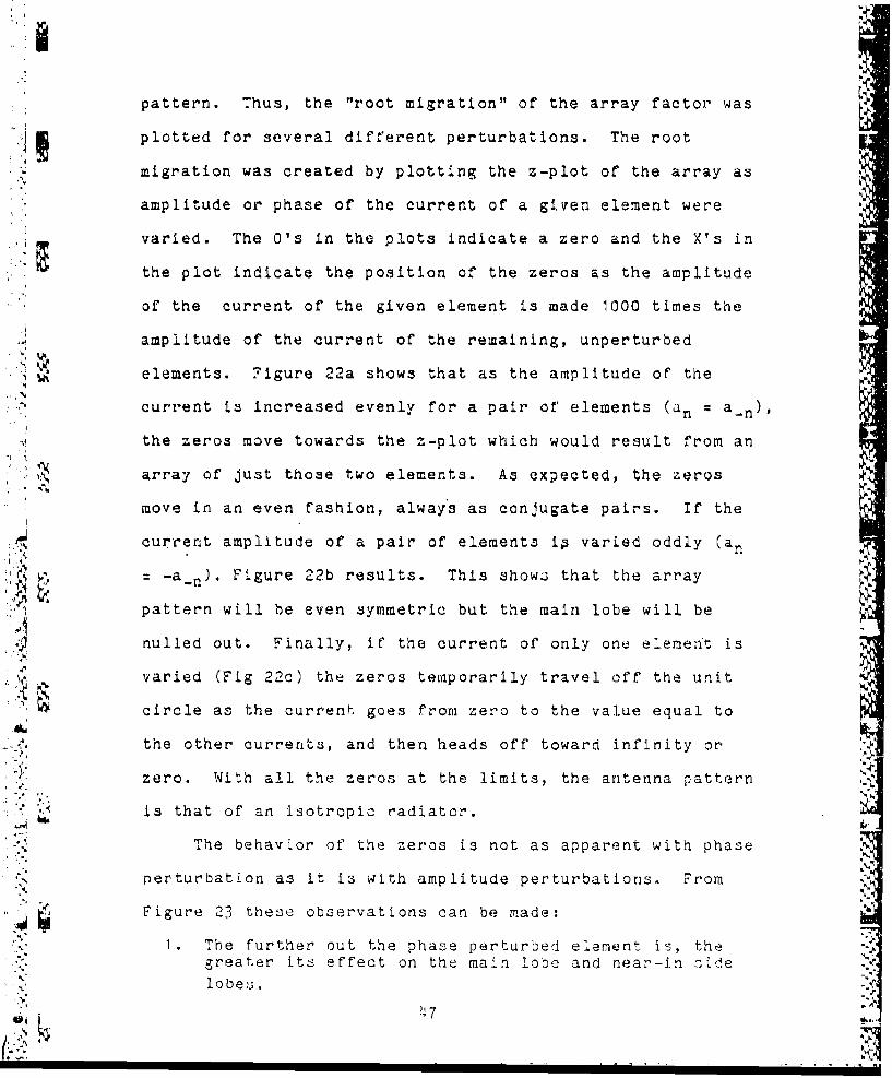
pattern. Thus, the "root migration" of the array factor was

plotted for several different perturbations. The root

migration was created by plotting the z-plot of the array as

amplitude or phase of the current of a given element were

varied. The O's in the plots indicate a zero and the X's in

the plot indicate the position of the zeros as the amplitude

of the current of the given element is made 1000 times the

amplitude of the current of the remaining, unperturbed

elements. Figure 22a shows that as the amplitude of the

current is increased evenly for a pair of elements (an an),

the zeros move towards the z-plot which would result from an

array of just those two elements. As expected, the zeros

move in an even fashion, alway's as conjugate pairs. If the

current amplitude of a pair of elements ip varied oddly (an

,-a_,n) Figure 22b results. This show. that the array

pattern will be even symmetric but the main lobe will be

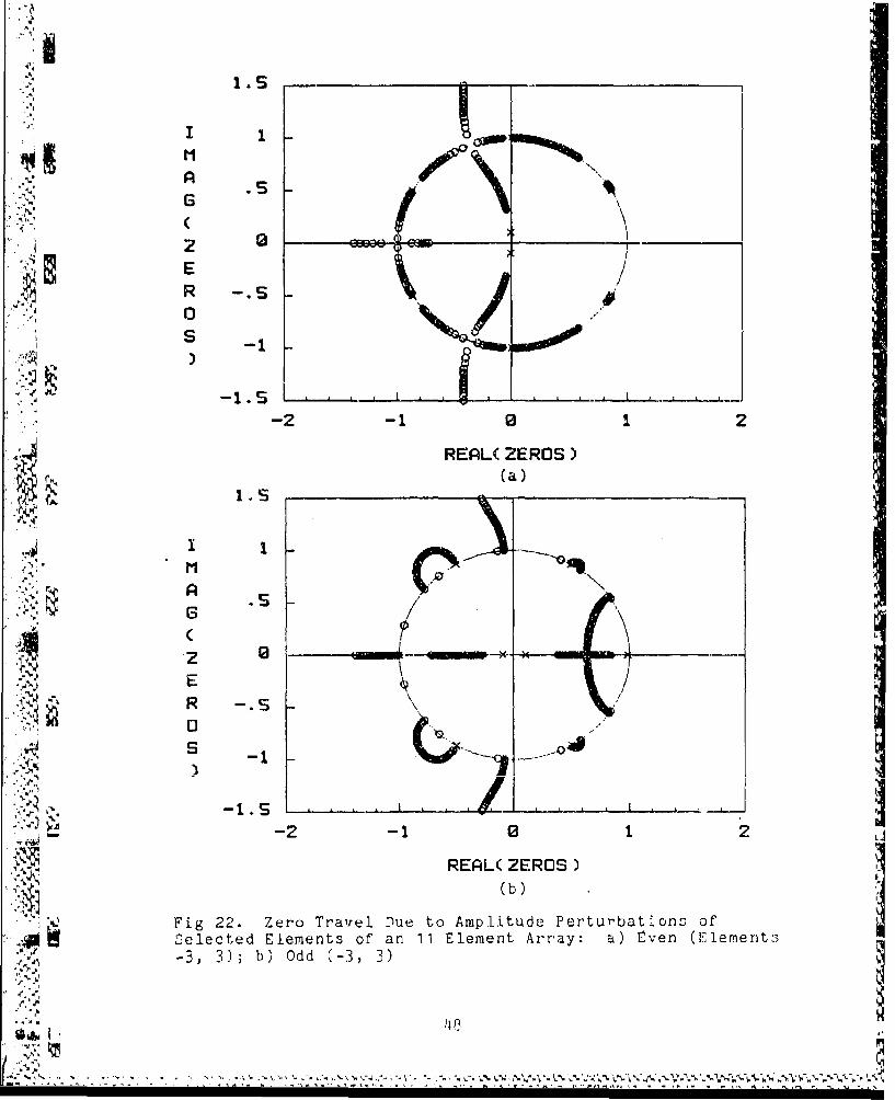
nulled out. Finally, if the current of only one element is

varied (Fig 22c) the zeros temporarily travel off the unit

circle as the current goes from zero to the value equal to

the other currents, and then heads off toward infinity or

zero. With all the zeros at the limits, the antenna pattern

is that of an isotropic radiator.

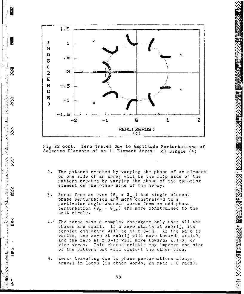
The behavior of the zeros is not as apparent with phase

Perturbation as it is with amplitude perturbations. From

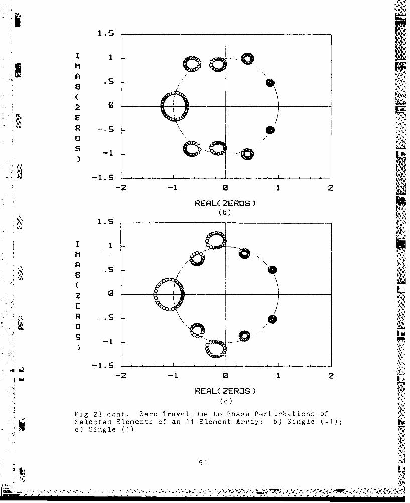
"Figure 23 these observations can be made:

1. The further out the phase perturbed element is, thegreater its effect on the main lobe and near-in :-delobe,-!

' %' 7

4.,; --

1.5-'

Ii 1aMA6

ER -.0

-2 -1 0 1 2

4 ~REAL( ZEROS)r (a)

.,.S

A

ER - O 3

0 -

-- 2 -1 0 1 2

REAL( ZEROS)(b)

Fig 22. Zero Travel Due to Amplitude Perturbation- ofSelect~ed Elements of an 11 Element Array: a) rven (Elements>

;b) Odd (-3, 3)

r. "(

,ji

2! 1 .51X

M

A SGX

22

E/R -. 5 -\

Ss, ~ ~~-1 x....

•- 1 .5 I • l . .. •. .... _ _... •

S-2 -1 2 1 2

REAL(ZEROS)

Fig 22 cont. Zero Travel Due to Amplitude Perturbations ofSelected Elements of an 11 Element Array: c) Single (4)

' 2. The pattern created by varying the phase of an elementon one side of an array will be the flip side of' thepattern created by varying the phase of the opposingelement on the other side of the array.

3. Zeros from an even (0n _n) and single elementphase perturbation are more constrained to aparticular angle whereas zeros from an odd phaseperturbation (Un = O-n) are more constrained to theunit circle.

J4. The zeros have a complex conjugate only when all thephases are equal. If a zero star'.s at z:O+lj, itscomplex conjugate will be at z=O-lj. As the parie isvaried, the zero at z=O+lj will move towards z:-1+O.j

• .".and the zero at z=O-lj will move towards z:1+0j orvice versa. This characteristic may improve one sideof the pattern but will distoct the other oide.

"",. Zeros traveling due to phase perturbations alwaystravel in loops (in other words, 2n rads = 0 rads).

4("

1.5

I I - R x~ 00o

0 0

S 04. 91ER 00

00

-1 0

-2 -1 1 2

.2 REAL( ZEROS)

Fig 23. Zero Travel Due to Phase Perturbations of SelectedElements of an 11 Element Array: a) Single (-5)

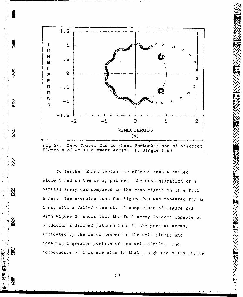
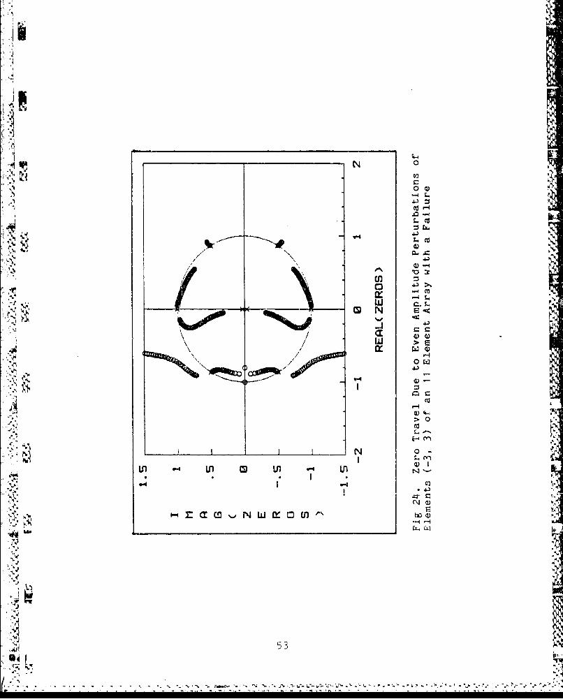
To further characterize the effects that a failed

element had on the array pattern, the root migration of a

I partial array was compared to the root migration of a full

array. The exercise done for Figure 22a was repeated for an

array with a failed elempnt. A comparlson of' Figure 22a

with Figure 24 shows that the full array is more capable of

producing a desired pattern than is the partial array,

indicated by the zeros nearer to the unit cir,'le and

lcovering a greater portion of the unit circle. The

consequence of this exercise is that though the nulls may be

"'Ir

1.SI I

R -. S

1 0

""- 0 1 2

!: ~REAL( 2EROS )(b

1.S U,

piIs/

6

E"R -. S50

-1-.

I w- 2 - 1 31ZI

""REAL( ZEROS)

* Fig 23 cont. Zero Travel Due to Phase Perturbations ofSelected Elements of an 11 Element Array: b) Single (-1);c) Single (1)

" "51

1.5

M

6 0~0000C 0

0 r2 0 1

E 000R -. S 0 00 /

0 f

S "

'..-2 - 2I-

-2- 0 10

i ~REAL( 2EROS )

1.•I 1 -

.•5 0o 0

00

i,.":" "'(•R -. 5SE 0000 0

X. R -1S L 0.~ A J I___S -1 -S

A' - . S . . . _ .. _, _ __ __ __. . . .._-2 -1 0I 1 2

REAL( ZEROS)

(e)

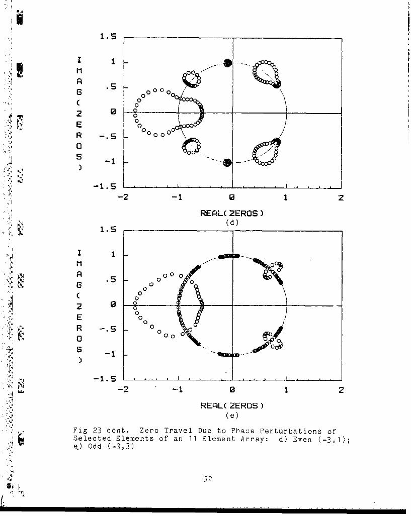
Fig 23 cont. Zero Travel Due to Fhase Perturbations ofSelected Elements of an 11 Element Array: d) Even (-3,1);q,) Odd (-3,3)

,•. 52

IIL

L(U

M N ,.-c

Ix w 4

>' /

N~ 0 ~ /N

ILI-

I I I N50

placed where desired, this would require a specific

amplitude distribut'on - a distribution which may require

"the failed elements to carry current. In other words, there

is a one-to-one mapping from the z-plot to the amplitude

distribution through the z-transform.

Results. The null displacement technique may be used

to optimize the pattern of an array by first determining all

possible zero locations and then choosing the aml, Ltude

distribution which corresponds to the best null positioning

or by first selecting the desired nulls and then with some

type of iterative program, converge to the best set of

available nulls. Either way, the advantage of this

technique, which is its potential speed in arriving at a

solution, is lost. This technique has an added disadvantage

,A '-in that it is difficult to determine whether or not the null

positions selected will actually create the best possible

4 pattern.

Iterative Techniques

Iterative techniques are those which first approximate

a solution, then compare the solution with some desired

criteria, and then approximate a new solution to be compared

until the solution matches the desired criteria. Of the

iterative techniques investigated; most noteably minimax

"7 •optimization, least mean square error optimization, and

steepest descent gradient search optimization, the latter bi

54

appeared to be the most applicable to the given problem.

The gradient search optimization technique can be used for

"arrays with arbitrary element positions and amplitude

distributions. The technique has the added advantage in

that the desired optimization criteria can be specified

exactly.

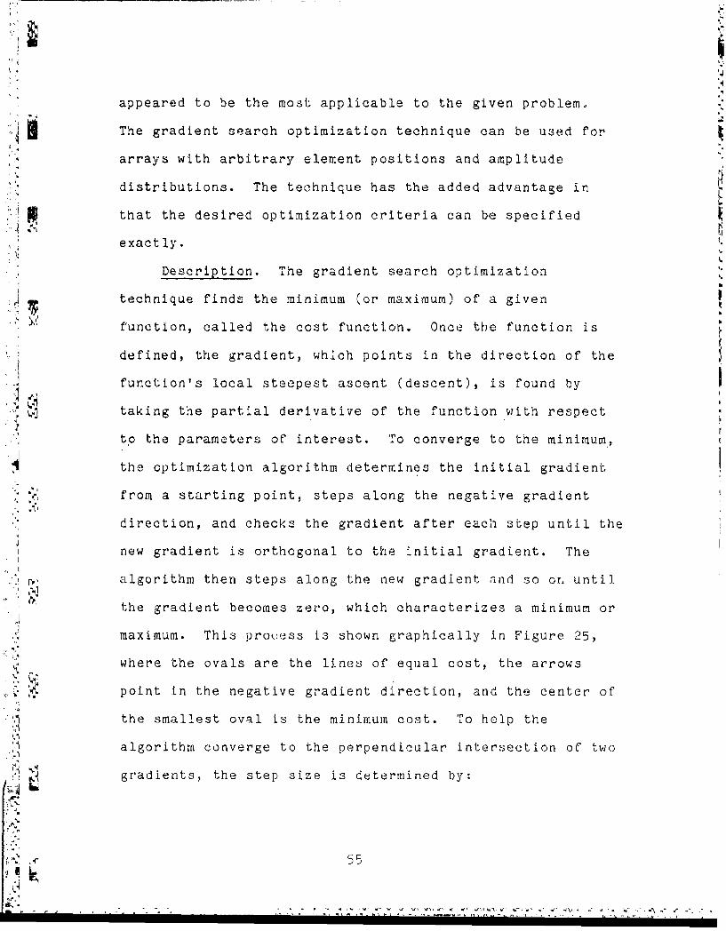
Description. The gradient search optimization

technique finds the minimum (or maximum) of a given

function, called the cost function. Once the function is

defined, the gradient, which points in the direction of the

function's local steepest ascent (descent), is found by

taking the partial derivative of the function with respect

to the parameters of interest. To converge to the minimum,

the optimization algorithm determines the initial gradient

"from a starting point, steps along the negative gradient

direction, and checks the gradient after each step until the

new gradient is orthogonal to the initial gradient. The

"algorithm then steps along the new gradient and so or. until

the gradient becomes zero, which characterizes a minimum or

maximum. This process is shown graphically in Figure 25,

where the ovals are the lines of equal cost, the arrows

point in the negative gradient direction, and the center of

the smallest oval is the minimum cost. To help the

algorithm converge to the perpendicular intersection of two

gradients, the step size is determined by:

55IL

CD

0

V a)0 a

-- ~ 0V. C..

ELI

OL 56)

new step = old step [I + 0.9 cos(v)]I.j

wlhere v is the angle between the initial gradient vector and

the new gradient vector. Inflection stationary points canr

be eliminated algorithmically. Although global optimality

is not guaranteed, experience and intuition help assure that.

the minimum reached I:5 optimal. This is especially true for

problems where the parameter space is tightly constrained by

physical limitations.

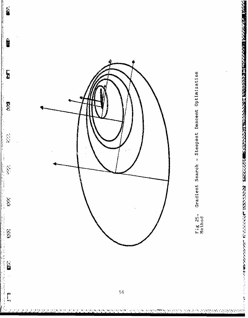
Application. The gradient search algorithm was

A programmed with the ADA programming language for a VAX

"11/780. The array used was an 101 element linear array.

The cost function which is to be optimized is described in

4 equation 9. The gradient vectors are:

N

, G/ 8ak : 2 am cos( 0 k-m) Hkm

j m=1

. ! ~and iiNandGN -2 ak am sin((k-om) Hkm

tm= 1

where am and 0. are the amplitude and phase, respectively,

of the current exciting element m. The optimization

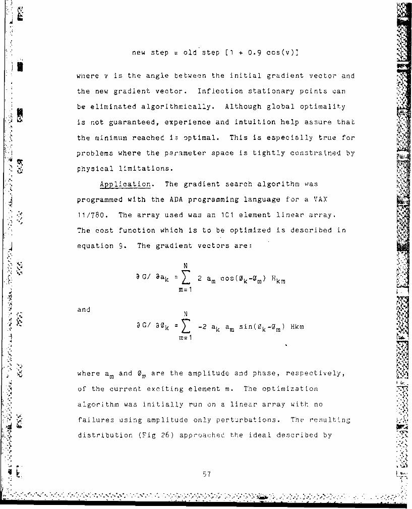
algorithm was initially run on a linear array with no

U failures using amplitude only perturbations. The resulting J

distribution (Fig 26) approached the ideal described by

• - . . .. ,.. 57V -. . -. .... %. .

""..,, P F -. -. -

°.02

•.01

.014.018

- ' .o14

"-K: .012

•i:;..cT .01

UD, ''• • D . 008

EJ.006

.004

"-4, ._o -_, , ____ _ _, , , , ,. _ , ,. . , , ,_-_

S-60 -40 -20 0 20 40 60

.N' A ELEMENT

.• Fig 26. Optimum Amplitude Distribution for Filled Array(Gradient Search Method)

~i ..2

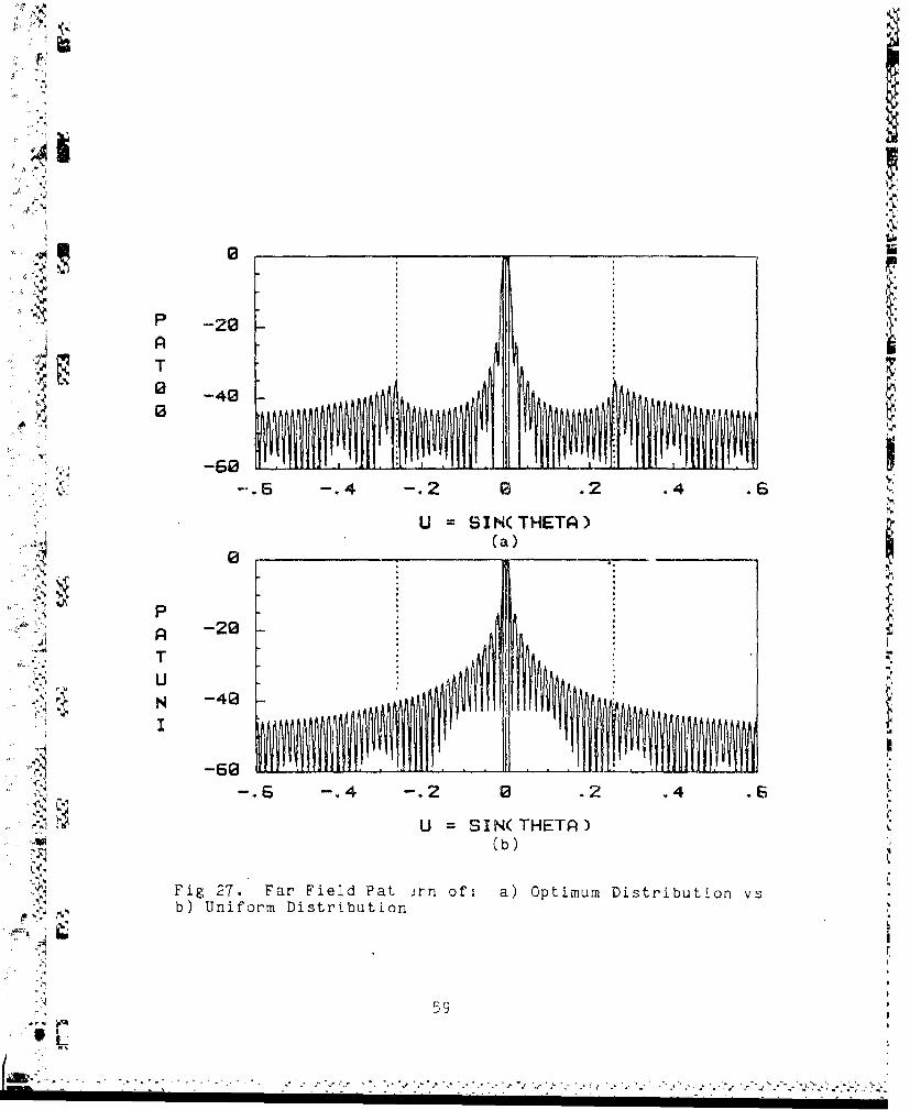
Y ,.

AI

0--. -. 4 -. 2 _2 .2 .4 ._

.,"13U SIN(THETA)

""P -20

T

,N -40

II

-:! -.6 -. 4 -. 2 0 .2 .4 .6

dr.

U = SIN(THETA)

-:V (b)

Fig 27. Far Field Pat .rn of. a) Optimum Distribution vs

.•,,•....,b) Uniform Distribution

,,.• 59

I "

- ...-... . .. 0 .2 ,. _ . 6

u uI I"l . .

'I*1 .62

•' .015

L

TU .00D _

"E . r. 5

-60 -40 -20 0 20 40 60

ELEMENT9 . ___________________(a)__________

P -20AT

:3

I ,

-60- o.-.4 . 2 .•94 .6

U : SIN(THETA)(b)

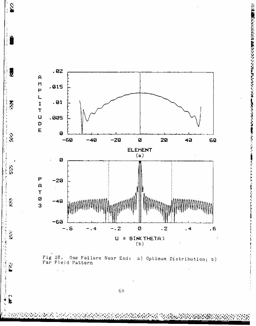
Fig 28. One Failure Near End: a) Optimum Distribution; b)Far, Field Pattern

"*1

'.] t 60

PL

S I .01

TU . GGN yUVD

-60 -40 -20 0 20 40 s6

ELEMENT

P -20.

T

IT -60

-. 6 -. 4 -. 2 0 .2 ..

"Pm U = SIN(THETA)(b)

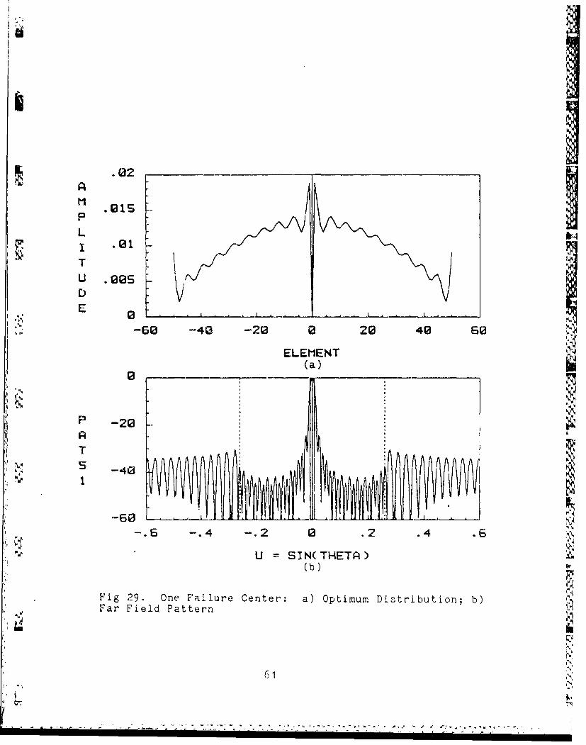
Fig 29. One Failure Center: a) Optimum Distribution; b)Far Field Pattern

61M i

-. . .. - . . . . . . . . .,,-. .14-

" .0

A-. 0

PM L

L

T* - U *0 10

D

"", -60 -40 -20 0 20 40 60

ELEMENT(a)

. -20

T

F,•L -403

"2

""�"-.6 -. 4 -. 2 64 G

U SIN(THETA)

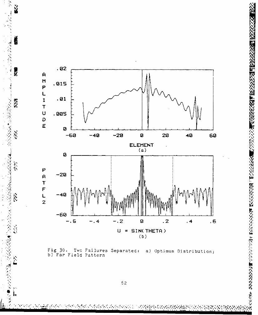
Fig 30. Two Failures Separated: a) Optimum Distribution;

b) Far' Field Pattern I

62

. %

• . •* .

•m,= V.

UUII

D

-60 -40 -20 0 20 40 s0

ELEMELNT(a)

0

-96

-. - -,- ' .2 ..

'-'-.6 -. 4 -. 2I 0 2G .4 .6

U =SIN(THETA)

(b

,''p

Ficg 31.ITen Failures Together: a) Optimum Distribution; b)Far Field Patt

>'3

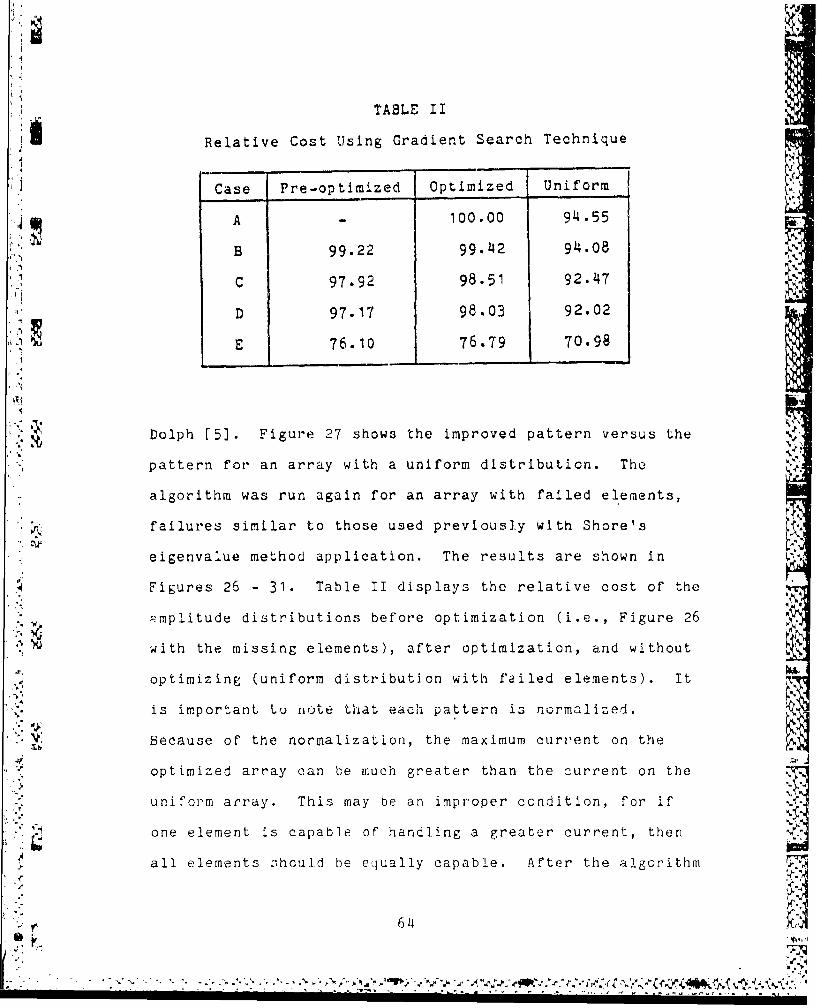
TABLE II

Relative Cost Using Gradient Search Technique

Case Pre-optimized Optimized Uniform J.

A 100.00 94.55

B 99.22 99.42 94.08

C 97.92 98.51 92.47

D 97.17 98.03 92.02

E 76.10 76.79 70.98

Dolph [5]. Figure 27 shows the improved pattern versus the

pattern for an array with a uniform distribution. The

algorithm was run again for an array with failed elements,

failures similar to those used previously with Shore's

eigenvalue method application. The results are shown in

Figures 26 - 31. Table II displays the relative cost of the

] mplitude distributions before optimization (i.e ., Figure 26

with the missing elements), after optimization, and without

optimizing (uniform distribution with failed elements). It

is important to note that each pattern is normalized.

Because of the norwalization, the maximum current on the

optimized array can be much greater than the current on the

uniform array. This may be an improper condition, for if

,one element is capable of handling a greater current, then

all elements Thould be equally capable. After the algorithm

64 X64

• r•-A.

J-31 • •.

was modified to constrain the amplitude of the current on

each individual element, the tests were repeated. In each

in order to minimize the cost function, all elements should

be at their maximum current handling capabilities. Only in

the case of limited total power available should amplitude

tapering (as a form of power management) be used.

Optimizing the antenna pattern using phase only

perturbations has been done by Voges and Butler [18] and

Shore [16]. For this study, the same gradient search

technique was us3ed for phase only optimization as was used

for amplitude only optimization. The result of running

cases a through e with phase only perturbations is that the

cost function was optimized when the phases of all the

elements were the same. The major reason for this is that

the area of interest is relatively large and is

even-symmetric, but from the root locus analysis, it was

determined that phase perturbations cause odd symmetric

S3 changes in array patterns. This means that an improvement

on one side of the pattern will cause a degradation on the

other side of the pattern. If the area of interest wasn't

so large, optimization may occur [161 using non-zero phase

shifts.

Results. The gradient search technique can be used to

optimize a phased array with failed elements. In fact the

solutions derived appear to be similar to the solutions

65

7,

lei

obtained with Shore's eigenvalue method. The reason for the

difference is that Shore was interested in minimizing the

amplitude perturbations, whereas the gradient search

"optimization method was run with a constraint on the total

current only. This technique did show that if the current

carrying capabilty of each element is constrained, the

optimum distribution would be an uniform distribution, but

if the total current available was constrained, the optimum

distribution would approach the Dolph-Chebyshev

"distribution. This technique also showed that for the case

of a complete element failure, phase perturbations would not

in'improve the pattern.

Direct Techni-que

The direct technique is a method which quickly arrives

at the optimum distribution for a partial array and is a

consequence of the results of the gradient search technique

and Shore's eigenvalue technique.-"J

Description. The direct method originated while trying

to find an even quicker optimization method. When

optimizing a very large array, with tens of thousands of

elements, the gradient search technique and the eigenvalue

@I technique may take a prohibil;'.vely long time. Inititally,

it was assumed that the compensation for failures involved

"mostly the elements in the proximity of the failure 7nd as a

result, only those elements needed to be included in the

66S b'-

- . --- - - - -

...

G1:

.02

M M.01S

IP

T-;, U *0S-

DE .

., ..,-60 -40 -2 0 20 40ELEMENT

.02

"2 •.- M .015

P4t L .01

U .005D

Ow W*-60 -42 -0220 40 60

ELEMENT(b)

Fig 32. Amplitude Distribution: a) Before and b) AfterOptimization I

A ~ 67

q. " ,

optimization analysis. To determine the required

compensation (comp), the difference between the

pre-optimized distribution and the optimized distribution

(Fig 32) for an 101 element array with the center element

failed was determined and is shown in Figure 33a. The iv

compensation was initially believed to be a Sa function

resulting from the inverse Fourier transform of what would-J undoubtably be the optimum pattern, a rect function centered

at u=O and with width 2Bw, and zero elsewhere in the FOV.

When this proved incorrect, curve fitting programs were

used. These proved fruitless and after Come sleuthing, it

¾]• was determined that the compensation is a scaled version of

the center row of the H matrix (Fig 33b). In general, a

failed element can be compensatod for- by simply adding a

scaled version of the corresponding row from the H matrix to

the remaining elements:

Wopt : 'fail + C,

where the elements of C are:

Cm s Hfm' with Cf: 0,

where C is a vector corresponding to the required

compensation for each element, f is the position index of

tbe failed element, m is the position index of the remaining

elements, and s is the scaLing which is proportional to the

original amplitude of the failed element.

Aplplication. The direct method can be applied by first

68

.. 2

C

p V- V 77

-610 -40 -20 0 20 40 60

ELEMENT

.2__a

R0

T -

,-':, p.1 -.-- .-- .. ............. A A A ,.....I. . .,

-60 -4G -20 0 20 40 60

ELEMENT(b)

SCa

F'ig 33. Compensation Required vs Row 0 of H- Matrix

S69

< - ---- -..- ---- -; .. -I -,2.- 40 -. , b,..J . -p.--- .

determining the optimum distribution for a full array, and

A then, when a failure occurs, simply calculating the required

compensation using equation 10 (H The scaling factor

will have to be pre-determined by running the gradient

"search program for each case. Once determtnd, it is then

multiplied by the compensation. The scaled compensation can

then be added to the pre-optimized distribution to arrive at

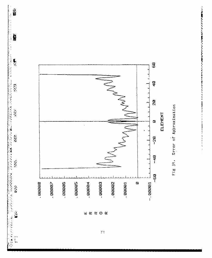
the optimum distribution. Figure 34 shows the difference

Ub'-ween the amplitude distributions generated by the direct

method and the gradien' search method.

Results. The direct optimization meshod is very quick

. • . an. simple to implement. Once the location of the failed

element is known, the power management system calculates the

.,.ompT,:satIon required to re-optimize the pattern, accesses

•I•!.?.i•the scal•.rg factov' frum a table, multipli-'es the compensation:v.i. .:,.+by tri- scaling factor, and then redistributes the available

power accordingly by adding the scaled compensation to the

2cur-"nts of the remaining elements.

.C,.

• ., ,.•o .,• -.

1..-

Al.

INI

>4o

Z ET

c_ _ _ N LO- I0 m m m c i--co 0rm C1 (M S) m (M ( mw

71"

'-4M

IV. Conclusions and Recommendations

Using a phased array antenna on a system can add

dimensions of flexibility and control. By varying the phase

and amplitude of the current exciting each element, the far

. field antenna pattern can be modified in such a way as to

obtain a desired, optimal pattern. The optimal pattern for

this study was defined as a pattern with minimal sidelobe

Spwer in a +/- 150 field of view and maximal main lobe power

within a given beam width. Although many methods for

optimizing the pattern of a full array are available, this

work is unique because it shows methods of finding the

optimum pattern of an array which contains failed or missing

elements. Optimization methods in the literature which were

investiga'ted include thinned array analysis, adaptive array

analysis, eigenvalue methods, null displacement techniques, Iand assorted iterative techniques. Another method discussed

in this thesis, the direct technique, originated from the

need for a quick optimization method, especially when very

large arrays are used.

4. 'A)-.

Conclusions

Of the optimization methods in the literature, only

Shore's eigenvalue method and the gradient search iterative

technique were sucessfully applied to thi:s problem. Of the

two techniques, Shole's eigenvalue technique is quicker and

more accurate (i.e., absolute convergence to the solution);

72

however, the gradient search technique is more flexible

(i.e., easier to change or add any constraints). For an

array with many elements neither technique is quick. The

direct method, a spin off from the solutions arrived at from

the eigenvalue method and the gradient search technique, has

been shown to be relatively quick and accurate. The direct

method is based on the fact that the amplitude perturbations

required to compensate for a failed element can be described

by a single equation (from the H matrix).

Recommen'. ti on s

There are two types of recommendations for future study

to be made: the first type involves improving the direct

optimization technique and the second type involves

considering more practical aspects of phased arrays.

. •The direct technique was developed through

experimentation with computer simulations. It is suggested

•;J that the resulting failure compensation and scaling factor

can be derived analytically. The equations netted through

such efforts should be flexible enough to include practical

conitrai.nts which are necessary for a realistic array.

A .The first practical recommendation is that the complete

.+ j optimization technique should converge to an amplitude

distribui Lon which limits the antenna's Q-factor and

maximizes the antenna's signal to noise ratio. It is well

Sknown that the Dolph-Chebyshev distribution, as was found in

4 4.. 73 7

, . i

" :-,,

the study, has an impractically high Q-factor. It has been

' 5 • suggested (8,9] that a Taylor R distribution provides the

"optimum distribution for a practical array. The Taylor R

distribution maintains a low Q-factor and controls the n

sidelobes near the main beam. The second practical

recommendation is to consider more realistic failures. For

instance, it is possible that the element may fail only

. ¶ partially - that the pha.se ,;hifter gets stuck at a certian

phase or that the amplitude merely becomes reduced instead

of being totally knocked out. Also, a failed element may.2JF. not become a matched load, as was assumed for the foregoing

study, but may become a short or open, thereby making mutual

coupling a more significant player in the problem. The

third practical recommendation is that it is necessary to

determine the effect which the final solution has on the

atenna's operational characteristics such as frequency

tolerante (bandwidth), scanning ability, and power

"efficiency. The final recommendation is to apply this work

to a planar array with other than isotropically radiating

elements.

711

Biblioga,

1. Applebaum, S.P. "Adaptive Arrays," IEEE Trans AntennaPropag., AP-24; 585-598 (September 1976).

2. Cheng, D.K. "Gain Optimization for Arbitrary AntennaArrays," IEEE Trans Antenna Propa__AP-13: 973-974(November 1965).

3. Compton, R.T., Jr. Adaptive Antenna Arrays Por AircraftCommunicaton Systems, ElectroScience Laboratory 309T-,AD 735096 (January 1972).

4. Davies, D.E.N. "Independent Angular Steering of EachZero Of the Directional Pattern for a Linear Array,"IEEE Trans Antenna Propag., AP-15: 296-298 (March

5. Dolph, C.L. "A Current Distribution for Broadside Arrayswhich Optimizes the Relationship Between Beam Width and

J Side-lobe Level," Proceedings of the IRE, 34: 335-348(June 1946).

6. Fenn, A.J., Engineer, Module calibrations via mutualcoupling. Telephone interview. Lincoln Laboratory,Massachusetts Insitute of Technolgy, 6 February 1986.

"7. Gaushell, D. "Synthesis of Linear Antenna Arrays UsingZ-Transforms, " IEEE Trans Antennas Propag., AP-19:75-80 (January 197-1).

8. Hansen, R.C., Antenna Systems Consultant, Realisticoptimum amplitude distributions. Personal Interview.R.C. Hansen, INC., Tarzana, CA, 18 September 1986.

"9. "Linear Arrays," Chapter 9 in The Handbook ofAntenna Design, Vol 2, edited by Rudge, A.W. et al,London, UK: Peregrinus Ltd., 1983.

10. Klein, C.A. "Design of Shaped-Beam Antennas throughMinimax Gain Optimization," IEEE Trans Antenna Propag.,AP-32: 963--968 (September 19-- ).

11. Lo, Y.T. "Random Periodic Arrays," Radio Cci., 3:425-436 (May 1968).

12. ----. "Optmization of Directivity and Signa].-to-NoiseRatio of an Arbitrary Antenna Array," Proceedings OfThe IEEE., Vol 54, No 8: 10.33-1045 (AuguP; 1966).•

13. Martins-Came].o, L. et al. "Linear Array Beam Shaping"Using Fletcher-Powell. Optimization," Proceed inGý of' 1_9 8f

"75

. . . ._,, - - -.-- -.- -

Antenna Conference held in Philadelphia: 395-398 (1986).

14. Schjaer-Jacobsen, H. and Madsen, K. "Synthesis ofNonuniformly Spaced Arrays using a General NonlnearMinimax Optimization Method," IEEE Trans AntennaPropag-, AP-24: 501-506 (July 1976).

15. Shore, Robert A. Sidelobe Sector Nulling With MinimizedWeight Perturbations, RADC-TR-85-56, AD A157-085 (March

16. ----. "Nulling at Symmetric Pattern Locations WithPhase-only Weight Control," IEEE Trans Antenna Propag.,AP-32: 530-533 (May 1984).

17. Skolnik, M.I. "Nonuniform Array," Chapter 6 in AntennaTheory, Part I, edited by Collin and Zucker, New York:McGraw Hill, 1969.

18. Steinberg, B.D. Principles ot Aperture and Array SystemDesign, New York: John Wiley and Sons, Inc., 1976.

19. Voges, R.C. and Butler, J.K. "Phased Optimization ofAntenna Array Gain with constrained AmplitudeExcitation," IEEE Trans Antenna Propag., AP-20: 432-436(July 1972).

.,/

•'.1

"L.5

VITA

in. Captain Dernard F. Collins II was born on 1 April 1960

in Offut AFB, Nebraska. He graduated from high school in

Mlton, New Hampshire, in 1978 and attended the University of

New Hampshire from which he received the degree of Bachelor

of Science in Electrical. Engineering in -June 1982. Upon

graduation, he received a commission in the USAF through the

ROTC program. He then served as an avionics systems

engineer on the electronic warfare system aboard the B-52

for the Systems Program Office for Strategic Systems,

Aeronautical Systems Division, Wright Patterson AFB, Ohio,

until entering the School of Engineering, Air Force

Institute of Technology, in May 1985.

Permanent address: 45 Charles St.

Milton, New Hampshire

03851

••-.4

, .'. *4*

.. . . .. . . . . . . . .. . . . . . . . . . . . . ,

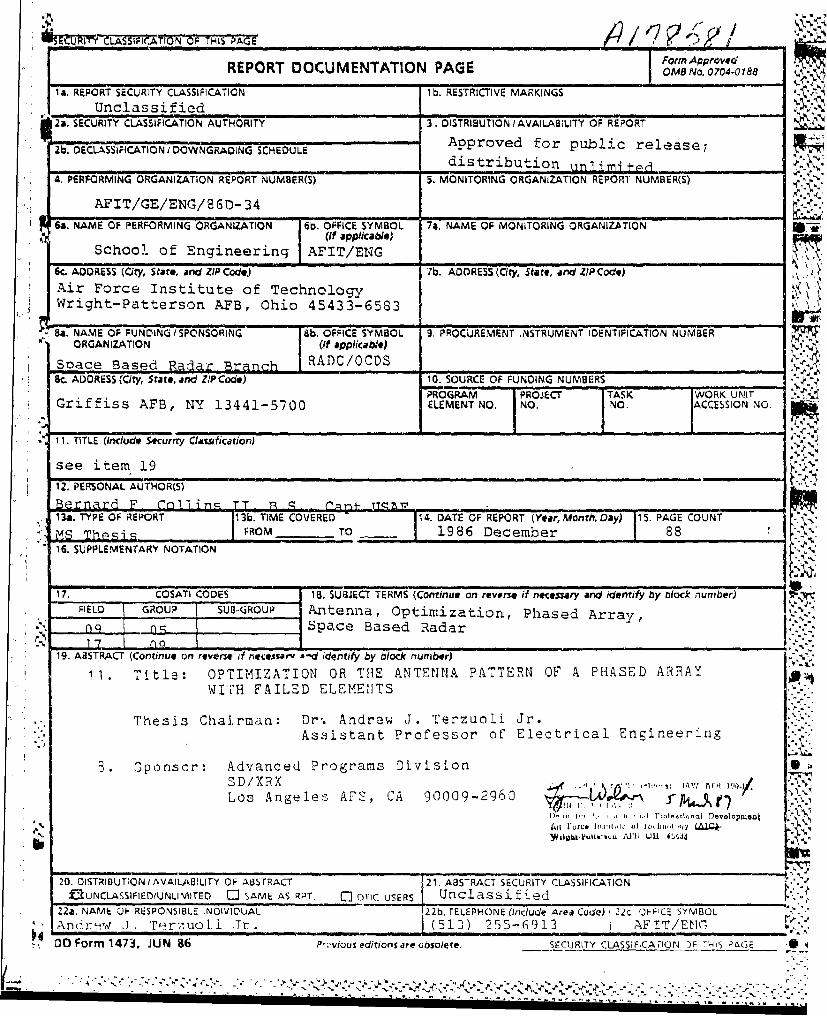
'IMSEURITY ILAS91FIC.ATION OF rT's PArE /~ K~ŽIREPORT DOCUMENTATION PAGE 08N.740188I.REPORT SECURITY CLASSIFICATION lb. RESTRICTIVE MARKINGSIl Unclassified____________ _______

2a. SECURITY CLASSIFICATION AUTHORITY 3. DISTRIBUTION IAVAIL.A8iLIY OF REPORT

2b. DECLASSIFICATION IDOWNGRADING SCHEDULE Approved for public release;______________________________ distribution_.i id

A.PERFORMING ORGANIZATION REPORT NUMBER(S) S. MONITORING ORGANIZATION REPORT NUMABER(S) .

AFIT/GE/ENG/860-34

6a. NAME OF PERFORMING ORGANIZATION 6b. OFFICE SYMBOL 7a. NAME OF MONITORING ORGANIZ-ATIONS(if applicable)

School of Engineering AFIT/ENG6.ADDRESS (Cry, State, and ZIP Code) 7b. ADDRESS (City, Start, and ZIP Cod*)Air Force Institute of Technology lAWright-Patterson AFB, Ohio 45433-6533

Ba. NAME OF FUNDING /SPC'NSORING 8b. OFrICE SYMBOL 9. PROCUREMENT NS~JTRUMENT IDENTIFICATION NUMBERORGANIZATION j(0f applicable) ~.,.

Soace Based RaTa rac RADC/OCDS8c. ADDRESS (City, Star*, and ZIP Code) 10. SOURCE OF FUNDING NUMBERS l

PROGRAM PROJECT TASK WORK UNITGrif fiss AFB, NY 13441-5700 ELEMENT NO. NO. NO. TACCE$SION NO. e

*. 11. TITLE (include Seocuri-ty Clazsication)

see item 1912. PERSONAL AUTHOR(S)

Bernard F. Coll1in-,T 1 ~(~~+-T~113a. TYPE OF REPORT 13b. TIME COVERED 14 DATE OF REPORT (Year, month, Day) 15. PAGE COUNT

ýS Thesi FROM____ -TO 198-eebr816. SUPPLEMENTARY NOTATION 1~ro

17. COSATI CODES 1B. SUBJECT TERMS (Continue on reverse if n~cesnary and identify by olock number)FIELD GROUP SUB-QROUP Antenna, Optimization, Phased Array,

nq n C;Space Based Radar

* 19. ABSTRACT (Continue on rovers@ if necostu"' x-d identify, by block nurmbor)

31. Tite: OPTI1M1IZATION OR THE ANTENNA PATTERN OF A PHASED ARRAYWIp'Mj FAILED ELEME11TS

Thesis Chairman: Dr. Andrew J. Terzuoli jr.Assistant Profezsor of Electrical Engineeri rg

3. ponsor: Advanced Programs Division -0iiSD! XR Xl', XViI

Los Angele~s AFS, CA 90009-2960 ~ ~ h~~I)" ~ JU U1 I rI lvopo

20. 0ISTRIfDUT;ON /AVAILABILITY OF ABSTRACT 21. ABSTRACT SECURITY CLASSIFICATIONf2UNCLASSIFIEDIUNLIMITED C3 SAME AS RPT. ~1OrIC USERS Unclassified

Z 2a. NAME OF RESPONSIBLE INDIVIDUAL 22b. TELEPHONE (includje Ared Codej) z22 OjFiCz SYMBOLr.-

AnciLq' LT. Ter7.ucti 7r. (513) 2 55-6 913 I AFIT/EýIC700 Form 1473, JUNJ 86 Prý'viaus editions are obsolete. -SC-CURITY C.LASSIl'iCAr[ON 01' -HIS ;)GE

19. Abstract

-' ' Using a phased array antenna on a system canadd dimensions of flexibility and control. Byvarying the phase and amplitude of the current"exciting each element, the far field antennapattern can be modified in such a way as to obtaina desired, optimal pattern. The purpose of thisthesis is to develop a rapid compensation methodfor any element failures by varying the currentsexciting the remaining elements. Although manymethods for optimizing the pattern of a full arrayare available, this work is unique because itdevelops methods of finding the optimum pattern ofan array which contains failed or missing

It elements. Optimization methods in the literature"which were investigated include thinned array"analysis, adaptive array analysis, eigenvaluemethods, null displacement techniques, andassorted iterative techniques. Another methoddiscussed in this thesis, the direc. technique,originated from the need for a quick optimizationmethod, especially when very large arrays areused.

Of the optimization methods in theliterature, only the eigenvalue method and thegradient search iterative technique weresuccessfully applied to this problem. The directmethod, a spin off from the eigenvalue method andthe gradient search technique, has been shown tobe relatively quick and accurate.

Recommendations for future study include thefunctional derivation describing the directoptimization method and including more practicalaspects of phased arrays in the propagation model.

\'.5

-. 5

?.5

2•A

.................. ...........................................