i. Definitions - The Oxford Q-Step Centre | About€¦ · Alex Williams- Q-step essay Does consensus democracy improve economic outcomes? Lijphart (2012, p295) argues that ‘consensus

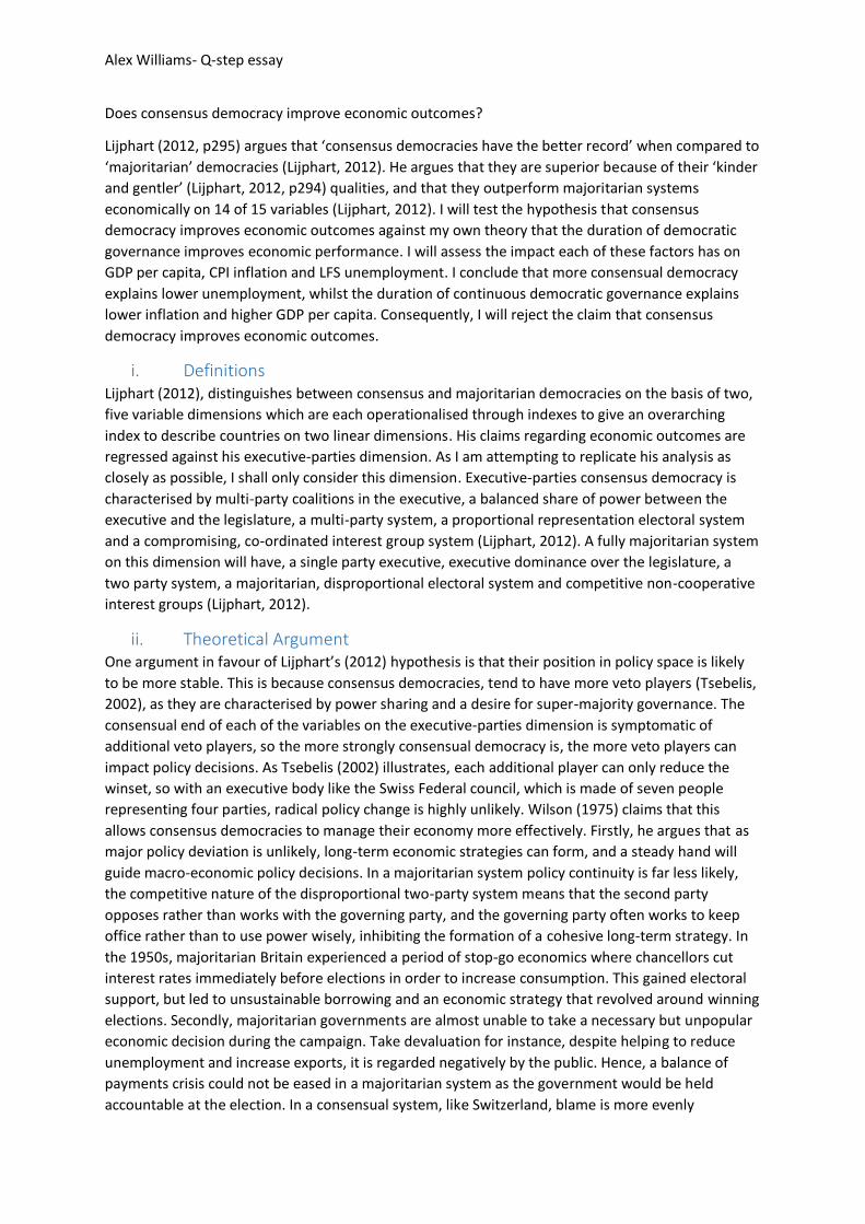
Alex Williams- Q-step essay

Does consensus democracy improve economic outcomes?

Lijphart (2012, p295) argues that ‘consensus democracies have the better record’ when compared to

‘majoritarian’ democracies (Lijphart, 2012). He argues that they are superior because of their ‘kinder

and gentler’ (Lijphart, 2012, p294) qualities, and that they outperform majoritarian systems

economically on 14 of 15 variables (Lijphart, 2012). I will test the hypothesis that consensus

democracy improves economic outcomes against my own theory that the duration of democratic

governance improves economic performance. I will assess the impact each of these factors has on

GDP per capita, CPI inflation and LFS unemployment. I conclude that more consensual democracy

explains lower unemployment, whilst the duration of continuous democratic governance explains

lower inflation and higher GDP per capita. Consequently, I will reject the claim that consensus

democracy improves economic outcomes.

i. Definitions Lijphart (2012), distinguishes between consensus and majoritarian democracies on the basis of two,

five variable dimensions which are each operationalised through indexes to give an overarching

index to describe countries on two linear dimensions. His claims regarding economic outcomes are

regressed against his executive-parties dimension. As I am attempting to replicate his analysis as

closely as possible, I shall only consider this dimension. Executive-parties consensus democracy is

characterised by multi-party coalitions in the executive, a balanced share of power between the

executive and the legislature, a multi-party system, a proportional representation electoral system

and a compromising, co-ordinated interest group system (Lijphart, 2012). A fully majoritarian system

on this dimension will have, a single party executive, executive dominance over the legislature, a

two party system, a majoritarian, disproportional electoral system and competitive non-cooperative

interest groups (Lijphart, 2012).

ii. Theoretical Argument One argument in favour of Lijphart’s (2012) hypothesis is that their position in policy space is likely

to be more stable. This is because consensus democracies, tend to have more veto players (Tsebelis,

2002), as they are characterised by power sharing and a desire for super-majority governance. The

consensual end of each of the variables on the executive-parties dimension is symptomatic of

additional veto players, so the more strongly consensual democracy is, the more veto players can

impact policy decisions. As Tsebelis (2002) illustrates, each additional player can only reduce the

winset, so with an executive body like the Swiss Federal council, which is made of seven people

representing four parties, radical policy change is highly unlikely. Wilson (1975) claims that this

allows consensus democracies to manage their economy more effectively. Firstly, he argues that as

major policy deviation is unlikely, long-term economic strategies can form, and a steady hand will

guide macro-economic policy decisions. In a majoritarian system policy continuity is far less likely,

the competitive nature of the disproportional two-party system means that the second party

opposes rather than works with the governing party, and the governing party often works to keep

office rather than to use power wisely, inhibiting the formation of a cohesive long-term strategy. In

the 1950s, majoritarian Britain experienced a period of stop-go economics where chancellors cut

interest rates immediately before elections in order to increase consumption. This gained electoral

support, but led to unsustainable borrowing and an economic strategy that revolved around winning

elections. Secondly, majoritarian governments are almost unable to take a necessary but unpopular

economic decision during the campaign. Take devaluation for instance, despite helping to reduce

unemployment and increase exports, it is regarded negatively by the public. Hence, a balance of

payments crisis could not be eased in a majoritarian system as the government would be held

accountable at the election. In a consensual system, like Switzerland, blame is more evenly


distributed so no one party risks being held accountable. It seems that having more veto players and

less direct accountability actually makes consensus democracies abler to form long term economic

plans. So Lijphart’s (2012) hypothesises is that consensus systems will have lower unemployment,

lower inflation and higher growth rates.

However, macroeconomic success may originate in states with a longer duration of democratic

government which have more experienced and embedded institutions. These systems give the

executive more past experience to draw on and also tend to see parties strategically converging on

the centre ground. For instance, Butskellism dominated British economic policy in the post-war

period as both parties endorsed similar economic policies. This means that each were close in policy

space and reduced the amount of deviation a change in governing party would bring. Thus, despite

majoritarian government, British macroeconomic policy was also characterised by stability. Whilst

Thatcher’s government represents a radical shift away from the status quo, the move right by New

Labour, led to macroeconomic continuity under Blair’s government. Thus, whilst Lijphart (2012)

claims that consensus democracies perform better on account of their stability, I argue that this

stability comes from embedded institutions that form based on the length of time a regime has been

democratic.

However, there are several major caveats to my argument. Firstly, globalisation, which works against

both my and Lijphart’s analysis, has led to greater macroeconomic interdependence between states.

Thus, domestic government policy is not the sole mechanism affecting macroeconomic

performance. Secondly, my analysis seems vulnerable to the argument that newer democracies can

draw on the historical experiences of older democracies and enact policy accordingly, so there is no

inherent advantage for older democracies. However, the political culture and sociological structure

of each state is different. One could not argue that linguistically divided Belgium could be governed

in the same manner as Britain, or learn massively from the history of Westminster democracy. Thus,

whilst this argument may have some gravity, it seems to imply that after twenty years each

democracy would be performing similarly and perusing identical policies. As this is not that case my

argument holds some validity.

iii. Empirical Evidence My empirical analysis uses the same thirty-six democracies as Lijphart’s (2012). This allows me to

test his hypothesis against mine using the same countries over the same period. Whilst Lijphart,

excludes the smallest five countries from his analysis of economic factors, I have included them. This

is because every country is vulnerable to external shocks, as the 2008 financial crisis showed, and to

maintain as much diversity as possible.

To operationalise the duration of continuous democratic rule, I have used a proxy measure based on

the year Lijphart (2012, p49) claimed a country became democratic for each country that was not

democratic before 1945. In all other cases I have used either 1945 or the year in which women

became fully enfranchised, unless the country was not independent at that point, as the point at

which the regime became democratic. So I have claimed that Finland has been democratic since

1918 when it gained independence from Russia. Likewise, the Republic of Ireland became

democratic in 1922. I then took the number of years before 2010 as my measure of the duration of

continuous democratic governance. Whilst imperfect this methodology will give an indication of

whether this is an explanatory variable.

Lijphart’s (2012) study, controls for both the logarithm of population size and the HDI when

assessing the impact of his executive-parties dimension on economic outcomes. I control for the


logarithm of population size to maintain consistency, but am unable to control for HDI as it is

strongly correlated with the age of democracy, the relationship is significant at the 0.1% level.

Inflation

Methodology

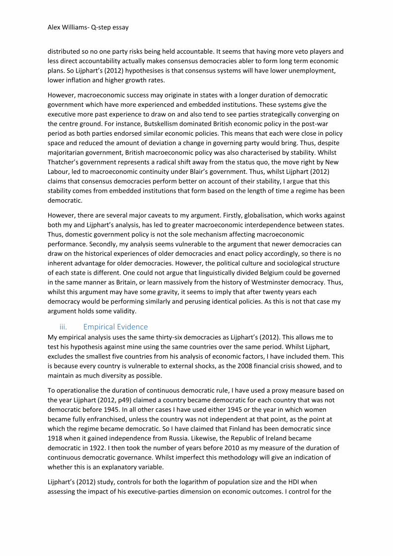
Following Lijphart’s (2012) example I have excluded Uruguay, Costa Rica and Jamaica from my

analysis of inflation as each of these countries experienced hyperinflation in this period, and are

statistical outliers. Botswana is also a statistical outlier, but as it did not experience hyper-inflation

and is included by Lijphart in his longer period, it has been included. I have compiled data from UN

data’s data base on average annual

CPI inflation and added it to

Lijphart’s (2012) dataset. This data

is given as an index where 2005 =

100, so I have taken the index

number for 2010 and divided it by

the 1991 value to produce a

number describing how much 1991

prices must be multiplied by to

reach 2010 prices.

Empirical results

Table 1: Regression between the duration of continuous democratic government up to 2010 and CPI inflation between 1991 and 2010 as measured by the UN.

Variables Executive-parties dimension 1981-2010 Duration of democratic governance Logarithm of population size Intercept N Adjusted R2

Model 1 Model 2 Model 3

Estimate (S.E)

-0.249** (0.129) 2.859 *** (0.309) 33 0.076

-0.112 (0.127) -0.014** (0.005) 2.761*** (0.329) 33 0.253

-0.111 (0.129) -0.014 ** (0.047) -0.021 (0.135) 2.845*** (0.639) 33 0.228

Level of statistical significance: p<0.001***, p<0.01**, p<0.05*

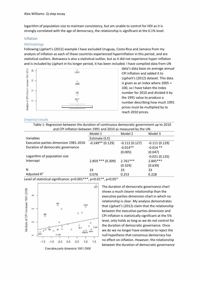
The duration of democratic governance chart

shows a much clearer relationship than the

executive parties-dimension chart in which no

relationship is clear. My analysis demonstrates

that Lijphart’s (2012) claim that the relationship

between the executive-parties dimension and

CPI inflation is statistically significant at the 5%

level, only holds as long as we do not control for

the duration of democratic governance. Once

we do we no longer have evidence to reject the

null hypothesis that consensus democracy has

no effect on inflation. However, the relationship

between the duration of democratic governance


and CPI inflation in this period is

statistically significant at the one percent

level even if we control for the logarithm

of population size. If we multiply the

regression coefficient by the standard

deviation, we find that a country that has

been democratic for an additional

standard deviation would have seen

inflation increase by a multiple of 0.381

less than a similar country that had been

democratic for one less standard

deviation. Hence, we have a regression

equation Y=2.845+-0.014X. This

relationship is significant at the 1%

level so is strong enough for us to

accept the hypothesis that the longer a regime is democratic for; the lower inflation it has.

Unemployment

Methodology

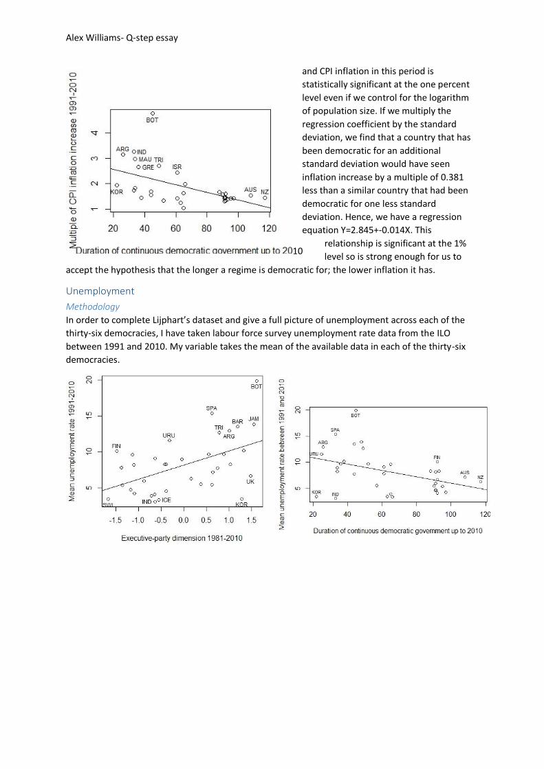
In order to complete Lijphart’s dataset and give a full picture of unemployment across each of the

thirty-six democracies, I have taken labour force survey unemployment rate data from the ILO

between 1991 and 2010. My variable takes the mean of the available data in each of the thirty-six

democracies.

10


Empirical results

Table 2: Regression between the duration of continuous democratic government up to 2010 and mean unemployment as measured by the ILO’s Labour Force Survey between 1991 and

2010.

Variables Executive-parties dimension 1981-2010 Duration of democratic governance Logarithm of population size Intercept N Adjusted R2


Estimate (S.E)

-1.974 **(0.572) 8.140*** (1.549) 36 0.237

-1.582* (0.596) -0.039 (0.022) 10.691*** (1.518) 36 0.284

-1.526* (0.593) -0.039 (0.022) -0.794 (0.643) 13.801*** (2.934) 36 0.296


Unlike my inflation data, these results suggest that there is a relationship between the executive-

parties dimension and an economic variable, when controlling for both the duration of continuous

democratic governance and the logarithm of 2009 population size. This relationship is statistically

significant at the 5% level, with the regression equation y=13.801-1.526x which is enough for us to

reject the null hypothesis that there is no relationship between the executive-parties measure of

consensus democracy and unemployment. Hence, we can conclude that there is such a relationship

and our regression coefficient of 1.526, and the standard deviation is one, we should expect

unemployment to be 1.53% lower in a country that became one standard deviation more

democratic. However, I cannot reject the null hypothesis that there is no relationship between the

length of time a regime has been democratic and unemployment, especially as several newer

democracies, like Korea, India and Botswana differ significantly from expectation as shown above.

Similarly, with the executive-parties index Botswana’s inflation is unexpectedly high and Korea’s

unexpectedly low, but the positive correlation is more evident.

GDP per capita

Methodology

As economic growth data is biased towards less developed rapidly industrialising economies, as

opposed to those already close to potential output, it is not a good variable to make long-run

economic comparisons from. Consequently, I have considered GDP per capita in 2010, which will

give a long term impression of how a regime has performed. I have sourced my data from UN stat. In

this regression I have controlled for a binary dummy variable where European countries are assigned

a one, which does not directly affect either of the outcomes of interest.

Empirical Results

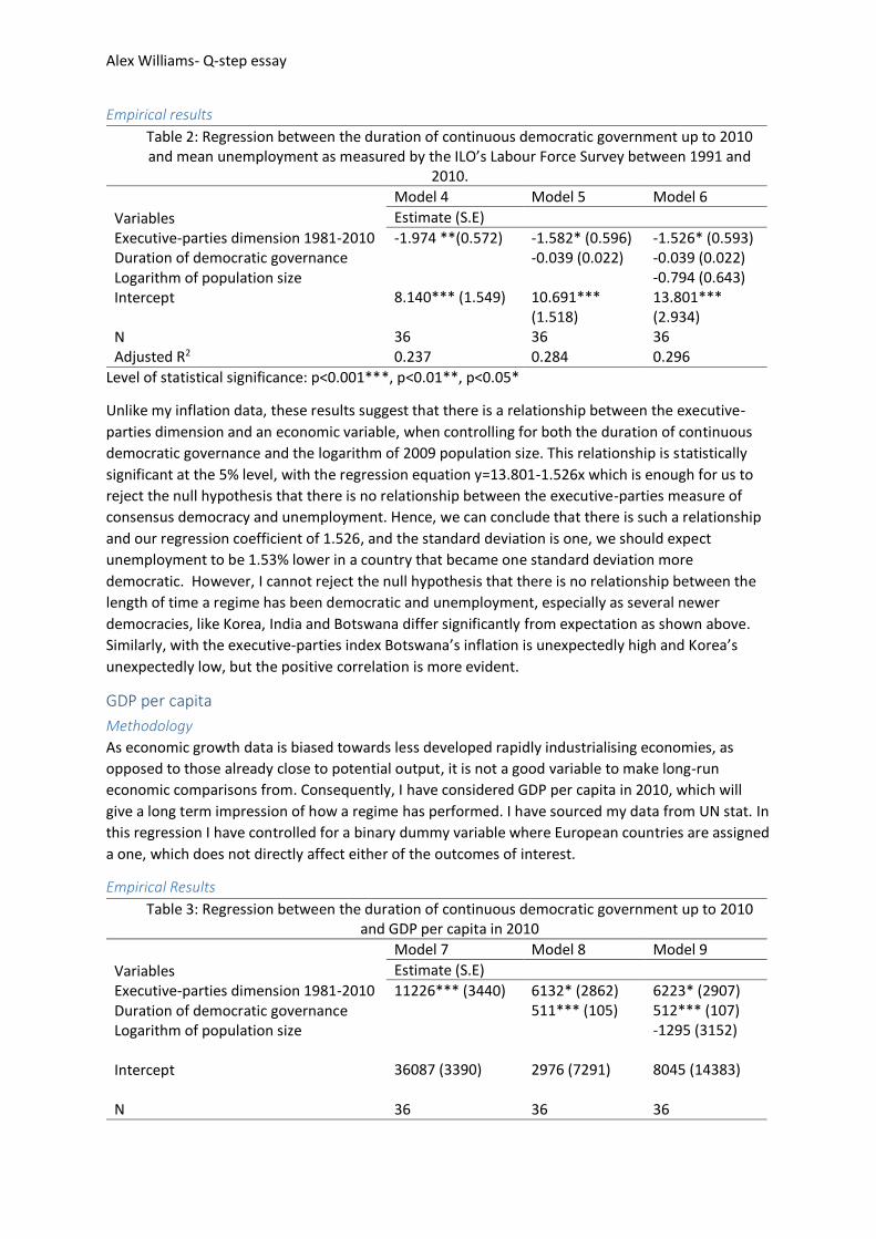
Table 3: Regression between the duration of continuous democratic government up to 2010 and GDP per capita in 2010

Variables Executive-parties dimension 1981-2010 Duration of democratic governance Logarithm of population size Intercept N


Estimate (S.E)

11226*** (3440) 36087 (3390) 36

6132* (2862) 511*** (105) 2976 (7291) 36

6223* (2907) 512*** (107) -1295 (3152) 8045 (14383) 36


Adjusted R2 0.216 0.530 0.518

Variables Executive-parties dimension 1981-2010 Duration of democratic governance Logarithm of population size Europe Intercept N Adjusted R2

Model 10

Estimate (S.E)

3235 (2999) 459*** (102) -691 (2959) 13904* (5883) 2194 (13677) 36 0.578


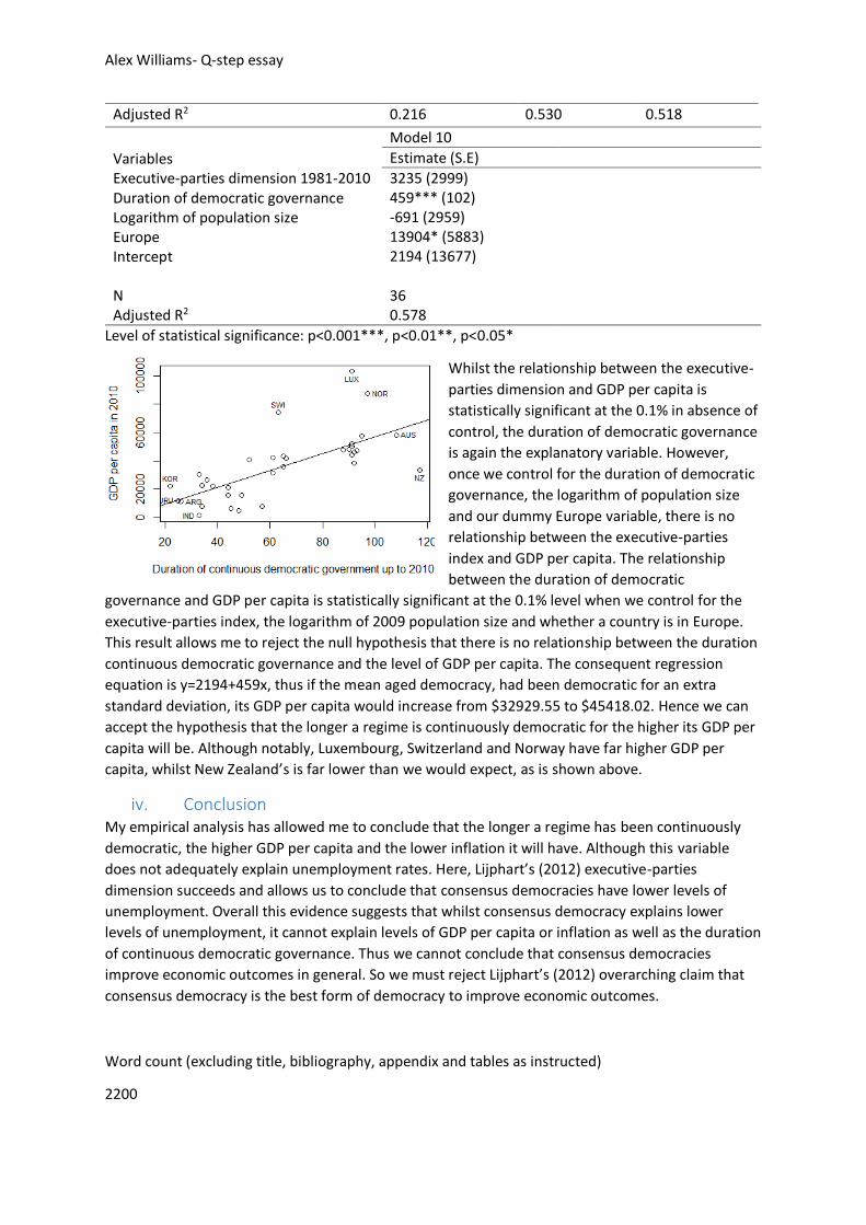
Whilst the relationship between the executive-

parties dimension and GDP per capita is

statistically significant at the 0.1% in absence of

control, the duration of democratic governance

is again the explanatory variable. However,

once we control for the duration of democratic

governance, the logarithm of population size

and our dummy Europe variable, there is no

relationship between the executive-parties

index and GDP per capita. The relationship

between the duration of democratic

governance and GDP per capita is statistically significant at the 0.1% level when we control for the

executive-parties index, the logarithm of 2009 population size and whether a country is in Europe.

This result allows me to reject the null hypothesis that there is no relationship between the duration

continuous democratic governance and the level of GDP per capita. The consequent regression

equation is y=2194+459x, thus if the mean aged democracy, had been democratic for an extra

standard deviation, its GDP per capita would increase from $32929.55 to $45418.02. Hence we can

accept the hypothesis that the longer a regime is continuously democratic for the higher its GDP per

capita will be. Although notably, Luxembourg, Switzerland and Norway have far higher GDP per

capita, whilst New Zealand’s is far lower than we would expect, as is shown above.

iv. Conclusion My empirical analysis has allowed me to conclude that the longer a regime has been continuously

democratic, the higher GDP per capita and the lower inflation it will have. Although this variable

does not adequately explain unemployment rates. Here, Lijphart’s (2012) executive-parties

dimension succeeds and allows us to conclude that consensus democracies have lower levels of

unemployment. Overall this evidence suggests that whilst consensus democracy explains lower

levels of unemployment, it cannot explain levels of GDP per capita or inflation as well as the duration

of continuous democratic governance. Thus we cannot conclude that consensus democracies

improve economic outcomes in general. So we must reject Lijphart’s (2012) overarching claim that

consensus democracy is the best form of democracy to improve economic outcomes.

Word count (excluding title, bibliography, appendix and tables as instructed)

2200


Bibliography

Lijphart, A., Patterns of Democracy: Government forms and performance in thirty-six democracies,

New Haven, 2012

Tsebelis, G., Veto Players – How Political Institutions Work, Princeton Unviersity Press, 2002.

Wilson, T., The Economic Costs of the Adversary System, printed in Finer, S.E., Adversary Politics and

Electoral Reform, 1975

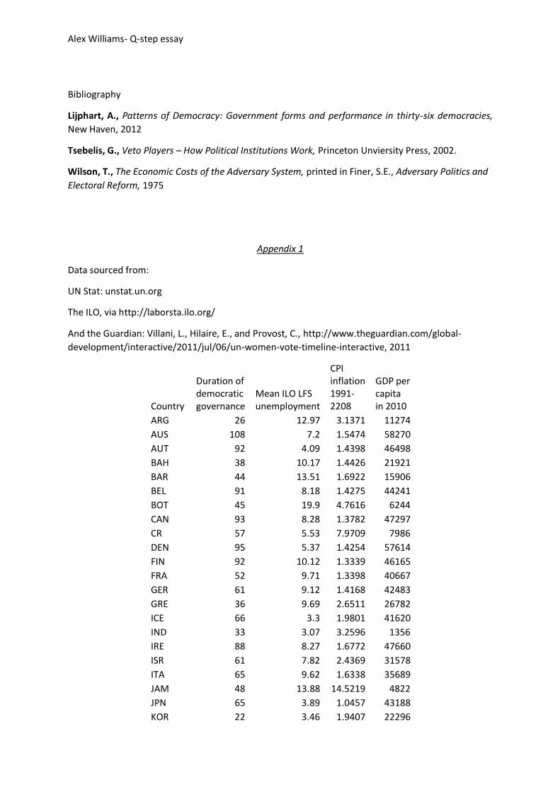
Appendix 1

Data sourced from:

UN Stat: unstat.un.org

The ILO, via http://laborsta.ilo.org/

And the Guardian: Villani, L., Hilaire, E., and Provost, C., http://www.theguardian.com/global-

development/interactive/2011/jul/06/un-women-vote-timeline-interactive, 2011

Country

Duration of democratic governance

Mean ILO LFS unemployment

CPI inflation 1991-2208

GDP per capita in 2010

ARG 26 12.97 3.1371 11274

AUS 108 7.2 1.5474 58270

AUT 92 4.09 1.4398 46498

BAH 38 10.17 1.4426 21921

BAR 44 13.51 1.6922 15906

BEL 91 8.18 1.4275 44241

BOT 45 19.9 4.7616 6244

CAN 93 8.28 1.3782 47297

CR 57 5.53 7.9709 7986

DEN 95 5.37 1.4254 57614

FIN 92 10.12 1.3339 46165

FRA 52 9.71 1.3398 40667

GER 61 9.12 1.4168 42483

GRE 36 9.69 2.6511 26782

ICE 66 3.3 1.9801 41620

IND 33 3.07 3.2596 1356

IRE 88 8.27 1.6772 47660

ISR 61 7.82 2.4369 31578

ITA 65 9.62 1.6338 35689

JAM 48 13.88 14.5219 4822

JPN 65 3.89 1.0457 43188

KOR 22 3.46 1.9407 22296


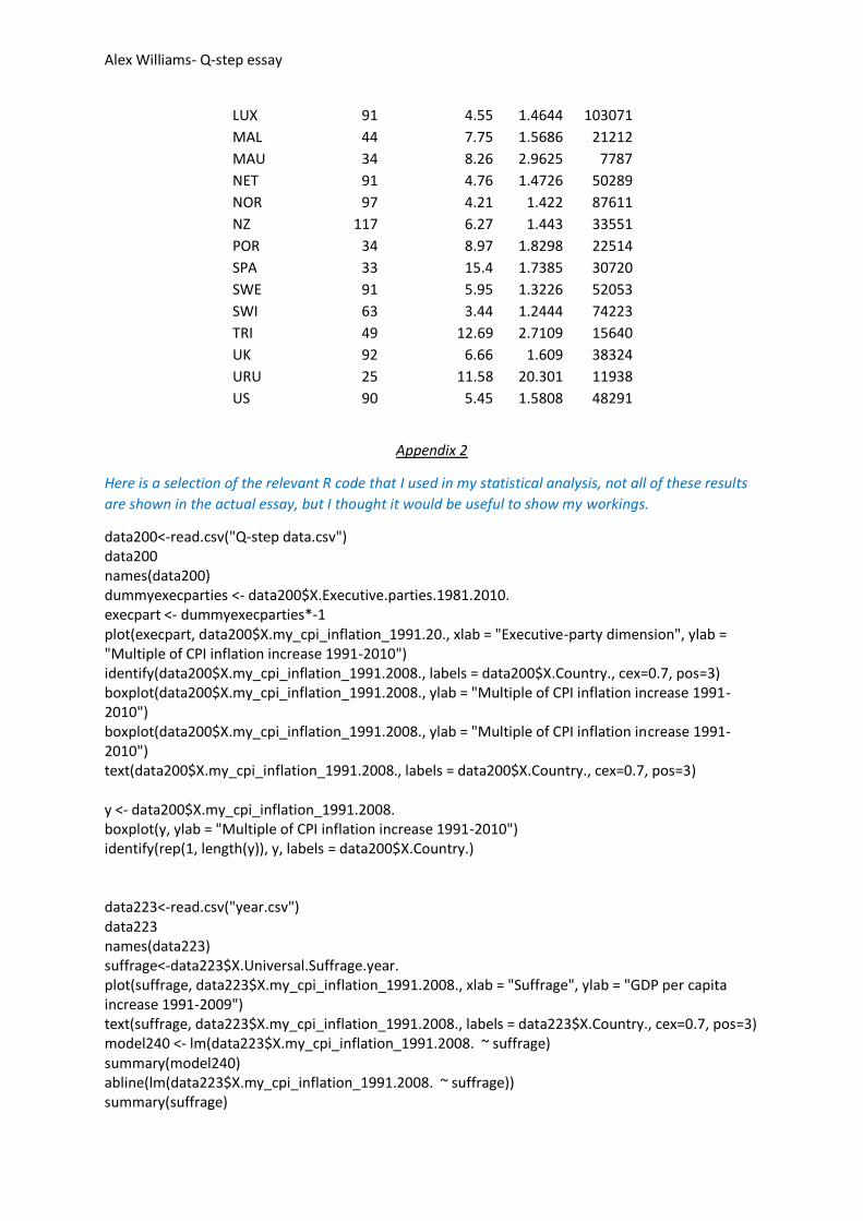
LUX 91 4.55 1.4644 103071

MAL 44 7.75 1.5686 21212

MAU 34 8.26 2.9625 7787

NET 91 4.76 1.4726 50289

NOR 97 4.21 1.422 87611

NZ 117 6.27 1.443 33551

POR 34 8.97 1.8298 22514

SPA 33 15.4 1.7385 30720

SWE 91 5.95 1.3226 52053

SWI 63 3.44 1.2444 74223

TRI 49 12.69 2.7109 15640

UK 92 6.66 1.609 38324

URU 25 11.58 20.301 11938

US 90 5.45 1.5808 48291

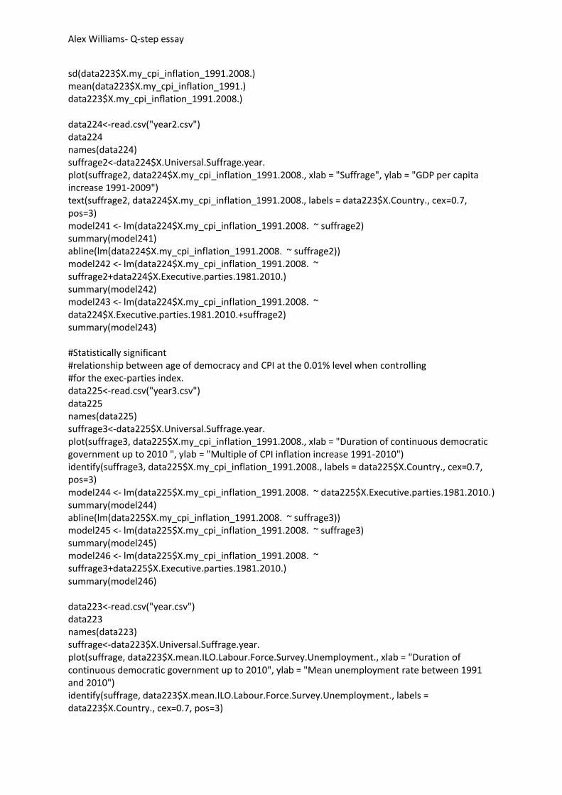
Appendix 2

Here is a selection of the relevant R code that I used in my statistical analysis, not all of these results

are shown in the actual essay, but I thought it would be useful to show my workings.

data200<-read.csv("Q-step data.csv") data200 names(data200) dummyexecparties <- data200$X.Executive.parties.1981.2010. execpart <- dummyexecparties*-1 plot(execpart, data200$X.my_cpi_inflation_1991.20., xlab = "Executive-party dimension", ylab = "Multiple of CPI inflation increase 1991-2010") identify(data200$X.my_cpi_inflation_1991.2008., labels = data200$X.Country., cex=0.7, pos=3) boxplot(data200$X.my_cpi_inflation_1991.2008., ylab = "Multiple of CPI inflation increase 1991-2010") boxplot(data200$X.my_cpi_inflation_1991.2008., ylab = "Multiple of CPI inflation increase 1991-2010") text(data200$X.my_cpi_inflation_1991.2008., labels = data200$X.Country., cex=0.7, pos=3) y <- data200$X.my_cpi_inflation_1991.2008. boxplot(y, ylab = "Multiple of CPI inflation increase 1991-2010") identify(rep(1, length(y)), y, labels = data200$X.Country.) data223<-read.csv("year.csv") data223 names(data223) suffrage<-data223$X.Universal.Suffrage.year. plot(suffrage, data223$X.my_cpi_inflation_1991.2008., xlab = "Suffrage", ylab = "GDP per capita increase 1991-2009") text(suffrage, data223$X.my_cpi_inflation_1991.2008., labels = data223$X.Country., cex=0.7, pos=3) model240 <- lm(data223$X.my_cpi_inflation_1991.2008. ~ suffrage) summary(model240) abline(lm(data223$X.my_cpi_inflation_1991.2008. ~ suffrage)) summary(suffrage)


sd(data223$X.my_cpi_inflation_1991.2008.) mean(data223$X.my_cpi_inflation_1991.) data223$X.my_cpi_inflation_1991.2008.) data224<-read.csv("year2.csv") data224 names(data224) suffrage2<-data224$X.Universal.Suffrage.year. plot(suffrage2, data224$X.my_cpi_inflation_1991.2008., xlab = "Suffrage", ylab = "GDP per capita increase 1991-2009") text(suffrage2, data224$X.my_cpi_inflation_1991.2008., labels = data223$X.Country., cex=0.7, pos=3) model241 <- lm(data224$X.my_cpi_inflation_1991.2008. ~ suffrage2) summary(model241) abline(lm(data224$X.my_cpi_inflation_1991.2008. ~ suffrage2)) model242 <- lm(data224$X.my_cpi_inflation_1991.2008. ~ suffrage2+data224$X.Executive.parties.1981.2010.) summary(model242) model243 <- lm(data224$X.my_cpi_inflation_1991.2008. ~ data224$X.Executive.parties.1981.2010.+suffrage2) summary(model243) #Statistically significant #relationship between age of democracy and CPI at the 0.01% level when controlling #for the exec-parties index. data225<-read.csv("year3.csv") data225 names(data225) suffrage3<-data225$X.Universal.Suffrage.year. plot(suffrage3, data225$X.my_cpi_inflation_1991.2008., xlab = "Duration of continuous democratic government up to 2010 ", ylab = "Multiple of CPI inflation increase 1991-2010") identify(suffrage3, data225$X.my_cpi_inflation_1991.2008., labels = data225$X.Country., cex=0.7, pos=3) model244 <- lm(data225$X.my_cpi_inflation_1991.2008. ~ data225$X.Executive.parties.1981.2010.) summary(model244) abline(lm(data225$X.my_cpi_inflation_1991.2008. ~ suffrage3)) model245 <- lm(data225$X.my_cpi_inflation_1991.2008. ~ suffrage3) summary(model245) model246 <- lm(data225$X.my_cpi_inflation_1991.2008. ~ suffrage3+data225$X.Executive.parties.1981.2010.) summary(model246) data223<-read.csv("year.csv") data223 names(data223) suffrage<-data223$X.Universal.Suffrage.year. plot(suffrage, data223$X.mean.ILO.Labour.Force.Survey.Unemployment., xlab = "Duration of continuous democratic government up to 2010", ylab = "Mean unemployment rate between 1991 and 2010") identify(suffrage, data223$X.mean.ILO.Labour.Force.Survey.Unemployment., labels = data223$X.Country., cex=0.7, pos=3)


model247 <- lm(data223$X.mean.ILO.Labour.Force.Survey.Unemployment. ~ data223$X.Executive.parties.1981.2010.) summary(model247) abline(lm(data223$X.mean.ILO.Labour.Force.Survey.Unemployment. ~ suffrage)) summary(suffrage) model248 <- lm(data223$X.mean.ILO.Labour.Force.Survey.Unemployment. ~ suffrage+data223$X.Executive.parties.1981.2010.+data223$X.Logarithm.of.2009.population.) summary(model248) model1000 <- lm(data223$X.HDI.2010.~suffrage) summary(model1000) plot(suffrage, data223$X.HDI.2010.) model271 <- lm(data223$X.mean.ILO.Labour.Force.Survey.Unemployment. ~ suffrage+data223$X.Executive.parties.1981.2010.) summary(model271) model272 <- lm(data223$X.mean.ILO.Labour.Force.Survey.Unemployment. ~ suffrage+data223$X.Executive.parties.1981.2010.+data223$X.Logarithm.of.2009.population.) summary(model272) model250 <- lm(data223$X.Executive.parties.1981.2010. ~ suffrage + data223$europe) summary(model250) data223<-read.csv("year.csv") data223 names(data223) suffrage<-data223$X.Universal.Suffrage.year. cap<-data223$X.tiger. plot(suffrage, cap, xlab = "Duration of continuous democratic government up to 2010 ", ylab = "GDP per capita in 2010") identify(suffrage, cap, labels = data223$X.Country., cex=0.7, pos=3) model250 <- lm(cap ~ data223$X.Executive.parties.1981.2010.) summary(model250) abline(lm(cap ~ suffrage)) model251 <- lm(cap ~ data223$X.Executive.parties.1981.2010. + suffrage) summary(model251) model252 <- lm(cap ~ suffrage+data223$X.Executive.parties.1981.2010.+data223$X.Logarithm.of.2009.population.) summary(model252) model252 <- lm(cap ~ suffrage+data223$X.Executive.parties.1981.2010.+data223$X.Logarithm.of.2009.population.+data223$europe) summary(model252) model252 <- lm(cap ~ suffrage+data223$X.Executive.parties.1981.2010.+data223$X.Logarithm.of.2009.population.+data223$europe+data223$X.EIU.democracy.index.) summary(model252) model252 <- lm(cap ~ suffrage+data223$X.Executive.parties.1981.2010.+data223$X.Logarithm.of.2009.population.+data223$europe+data223$X.EIU.democracy.index.) summary(model252) options(scipen = 5) summary(suffrage)


summary(lm(suffrage~data223$X.HDI.2010.)) e <- data223$X.Executive.parties.1981.2010.*-1 plot(data223$X.Executive.parties.1981.2010.*-1, cap, xlab = "Executive-party dimension 1981-2008", ylab = "GDP per capita in 2010") identify(data223$X.Executive.parties.1981.2010.*-1, cap, labels = data223$X.Country., cex=0.7, pos=3) model253 <- lm(cap~data223$X.Executive.parties.1981.2010.+data223$europe+data223$X.Logarithm.of.2009.population.) summary(model253) abline(lm(cap~e)) data223$europe = data223$X.Country. %in% c('AUT', 'BEL', 'DEN', 'FIN', 'FRA', 'GER', 'ICE', 'IRE', 'ITA', 'LUX', 'MAL', 'NET', 'NOR', 'POR', 'SPA', 'SWE', 'SWI', 'UK') data223$europe data223$medianage = data223$X.Country. %in% c('SWI', 'JPN', 'ITA', 'ICE', 'IRE', 'US', 'SWE', 'NET', 'LUX', 'BEL', 'UK', 'FIN', 'AUT', 'CAN', 'DEN', 'NOR', 'AUS', 'NZ') data223$medianage = data223$X.Country. %in% C('SWI', 'JPN', 'ITA', 'ICE', 'IRE', 'US', 'SWE', 'NET', 'LUX', 'BEL', 'UK', 'FIN', 'AUT', 'CAN', 'DEN', 'NOR', 'AUS', 'NZ') medianage <- data223$medianage model544 <- lm(cap~medianage) summary(model544) medianage model543 <- lm(cap~suffrage, data = data[!medianage,]) summary(model543) plot(cap~suffrage, data = data[!medianage,]) medianage1 = C('SWI', 'JPN', 'ITA', 'ICE', 'IRE', 'US', 'SWE', 'NET', 'LUX', 'BEL', 'UK', 'FIN', 'AUT', 'CAN', 'DEN', 'NOR', 'AUS', 'NZ') mean(suffrage) sd(suffrage) mean(data200$X.my_cpi_inflation_1991.2008.) sd(data200$X.my_cpi_inflation_1991.2008.) IQR(data200$X.my_cpi_inflation_1991.2008.) model201 <- lm(data200$X.My_GDP_1991.2009. ~ execpart) summary(model201) abline(lm(data200$X.My_GDP_1991.2009. ~ execpart)) model232 <- lm(data200$X.My_GDP_1991.2009. ~ execpart+data200$X.Logarithm.of.2009.population.) summary(model232) sd(execpart) plot(execpart, data200$X.my_cpi_inflation_1991.2008, xlab = "Executive-party dimension", ylab = "CPI inflation multiplicator") identify(execpart, data200$X.my_cpi_inflation_1991.2008, labels = data200$X.Country., cex=0.75, pos=3) model202 <- lm(data200$X.my_cpi_inflation_1991.2008 ~ execpart)


summary(model202) abline(lm(data200$X.my_cpi_inflation_1991.2008~execpart)) plot(execpart, data200$X.mean.ILO.Labour.Force.Survey.Unemployment., xlab = "Executive-party dimension 1981-2010", ylab = "Mean unemployment rate 1991-2010") identify(execpart, data200$X.mean.ILO.Labour.Force.Survey.Unemployment., labels = data200$X.Country., cex=0.75, pos=3) model203 <- lm(data200$X.mean.ILO.Labour.Force.Survey.Unemployment.~execpart+data200$X.Logarithm.of.2009.population.+data200$X.HDI.2010.) summary(model203) abline(lm(data200$X.mean.ILO.Labour.Force.Survey.Unemployment.~execpart)) #Even if we control for the log of population size and the level of development we still get a statistically significant result. model221 <- lm(data200$X.mean.ILO.Labour.Force.Survey.Unemployment.~execpart+data200$X.Logarithm.of.2009.population.) summary(model221) model222 <- lm(data200$X.mean.ILO.Labour.Force.Survey.Unemployment.~execpart) summary(model222) names(data201) plot(execpart, data201$cpi_1991_2009, xlab = "Executive-Parties Dimension", ylab = "Multiple of CPI inflation increase 1991-2009") text(execpart, data201$cpi_1991_2009, labels = data200$X.Country., cex=0.5, pos=3) model204 <- lm(data201$cpi_1991_2009~execpart+data201$pop_in_thousands_2009) summary(model204) abline(lm(data201$cpi_1991_2009~execpart)) #Dataset that excludes Uruguay, CR and Jamaica data202<-read.csv("DataminusURUJAM.csv") data202 names(data202) execpart2 <- data202$X.Executive.parties.1981.2010.*-1 plot(execpart2, data202$X.my_cpi_inflation_1991.2008, xlab = "Executive-party dimension 1981-2008", ylab = "Multiple of CPI increase 1991-2008") identify(execpart2, data202$X.my_cpi_inflation_1991.2008, labels = data202$X.Country., cex=0.7, pos=3) model205 <- lm(data202$X.my_cpi_inflation_1991.2008~execpart2+data202$X.Logarithm.of.2009.population.+data202$X.HDI.2010.) summary(model205) abline(lm(data202$X.my_cpi_inflation_1991.2008~execpart2)) model223 <- lm(data202$X.my_cpi_inflation_1991.2008~execpart2+data202$X.Logarithm.of.2009.population.) summary(model223)


model224 <- lm(data202$X.my_cpi_inflation_1991.2008~execpart2) summary(model224) data204<-read.csv("My dataset.csv") data204 plot(data204$X.Executive.parties.1981.2010., data204$X.mean.ILO.Labour.Force.Survey.Unemployment., xlab = "Plenary Agenda", ylab = "Mean unemployment") text(data204$X.Executive.parties.1981.2010., data204$X.mean.ILO.Labour.Force.Survey.Unemployment., labels = data204$X.Country., cex=0.5, pos=3) model211 <- lm(data204$X.mean.ILO.Labour.Force.Survey.Unemployment.~data204$X.Executive.parties.1981.2010.) summary(model211) abline(lm(data204$X.mean.ILO.Labour.Force.Survey.Unemployment.~data204$X.Executive.parties.1981.2010.)) data205<-read.csv("economicdata.csv") data205 names(data205) dummyexecpart6 <- data205$X.Executive.parties.1981.2010. execpart205 <- dummyexecpart6*-1 plot(execpart205, data205$X.My_GDP_1991.2009., xlab = "Executive-party dimension", ylab = "GDP per capita increase 1991-2009") text(execpart205, data205$X.My_GDP_1991.2009., labels = data205$X.Country., cex=0.5, pos=3) model212 <- lm(data205$X.My_GDP_1991.2009.~execpart205) summary(model212) abline(lm(data205$X.My_GDP_1991.2009.~execpart205)) plot(execpart205, data205$X.mean.ILO.Labour.Force.Survey.Unemployment., xlab = "Executive-party dimension", ylab = "mEAN UNEMPLOYMENT 1991-2009") text(execpart205, data205$X.mean.ILO.Labour.Force.Survey.Unemployment., labels = data205$X.Country., cex=0.5, pos=3) model213<- lm(data205$X.mean.ILO.Labour.Force.Survey.Unemployment.~execpart205) summary(model213) abline(lm(data205$X.mean.ILO.Labour.Force.Survey.Unemployment.~execpart205)) names(data200) model214<-lm(data200$X.my_cpi_inflation_1991.2008.~data200$X.Index.of.central.bank.independence.1981.1994.) summary(model214)


model2016 <- lm(data207$X.Change_in_GDP_per_capita_2008.2011.~execrisis+data207$X.Logarithm.of.2009.population.) summary(model2016) model2017 <- lm(data207$X.Change_in_GDP_per_capita_2008.2011.~execrisis+data207$X.Logarithm.of.2009.population.+data207$X.HDI.2010.) summary(model2017) lm(data200$X.mean.ILO.Labour.Force.Survey.Unemployment.~execpart+data200$X.Logarithm.of.2009.population.+data200$X.HDI.2010.)

Documents

i. Definitions - The Oxford Q-Step Centre | About€¦ · Alex Williams- Q-step essay Does consensus democracy improve economic outcomes? Lijphart (2012, p295) argues that ‘consensus