SPAAN FELLOWWorking Papersin Second or Foreign Language Assessment

MIC

H I GAN

••E

LI T E S T I N

G

VOLUME 2 2004

Spaan Fellow Working Papers in Second or Foreign Language Assessment

Volume 2

2004

Edited by

Jeff S. Johnson

Published by

English Language Institute University of Michigan

TCF Building

401 E. Liberty, Suite 350 Ann Arbor, MI 48104-2298

testpubs@umich.edu http://www.lsa.umich.edu/eli

First Printing, April, 2004 © 2004 by the English Language Institute, University of Michigan. No part of this document may be reproduced or utilized in any form or by any means, electronic or mechanical, including photocopying, recording, or by any information storage and retrieval system, without permission in writing from the publisher. The Regents of the University of Michigan: David A. Brandon, Laurence B. Deitch, Olivia P. Maynard, Rebecca McGowan, Andrea Fischer Newman, Andrew C. Richner, S. Martin Taylor, Katherine E. White, Mary Sue Coleman, ex officio

Errata    PAGE   FOR   READ  iii   Tobie  van  Dyk   Tobie  van  Dyk  &  Albert  Weideman  135   Tobie  van  Dyk   Tobie  van  Dyk  &  Albert  Weideman        Albert  Weideman  has  been  added  as  the  co-­‐author  for  the  paper  Switching  Constructs:  On  the  Selection  of  an  Appropriate  Blueprint  for  Academic  Literacy  Assessment  in  Volume  2  of  Spaan  Fellow  Working  Papers  in  Second  or  Foreign  Language  Assessment  (2004).  

Table of Contents Introduction . . . . . . . . . . . . . . . . . . . . . . . . . . . . . . . . . . . . . . . . . . . . . . . . . . . . iv Spaan Fellowship Information . . . . . . . . . . . . . . . . . . . . . . . . . . . . . . . . . . . . . vi Elvis Wagner

A Construct Validation Study of the Extended Listening Sections of the ECPE and MELAB . . . . . . . . . . . . . . . . . . . . . . . . . . . . . . . . . . . . . 1

Hong Jiao

Evaluating the Dimensionality of the Michigan English Language Assessment Battery . . . . . . . . . . . . . . . . . . . . . . . . . . . . . . . . . . . . . . . . . 27

Matthew S. Weltig Effects of Language Errors and Importance Attributed to Language

on Language and Rhetorical-Level Essay Scoring . . . . . . . . . . . . . . . . . 53 Xiaoming Xi

Investigating Language Performance on the Graph Description Task in a Semi-Direct Oral Test . . . . . . . . . . . . . . . . . . . . . . . . . . . . . . . . . . . 83

Tobie van Dyk & Albert Weideman Switching Constructs: On the Selection of an Appropriate Blueprint

for Academic Literacy Assessment . . . . . . . . . . . . . . . . . . . . . . . . . . . . 135

iii

Introduction This second issue of the Spaan Fellow Working Papers in Second or Foreign Language Assessment presents five papers written by the University of Michigan English Language Institute 2003 Spaan Fellows. Elvis Wagner tests the hypothesis that listening to extended discourse involves two measurable traits: listening for explicitly stated information and listening for implicit information. Wagner divided all the extended listening passage items from the ECPE and MELAB test batteries into explicit and implicit groups and then used exploratory factor analysis to determine if the two sets of items would load on separate factors. For both test batteries, however, both sets of items loaded together on a single factor, thus providing no evidence to support the hypothesis. Wagner then examined two-factor solutions for each of the test batteries, but the results again did not support the hypothesis, as the loadings for the explicit and implicit items were not clearly divided among the first and second factors. Wagner then examined a three-factor solution for the ECPE items and found that the items were text dependent. That is, items from each of the three extended listening texts in the test loaded on their own, separate factors. This result, while not supporting Wagner’s hypothesis, does suggest that the current practice of using a variety of fairly short extended passages is fairer, in terms of controlling for examinee background knowledge, than using a single, long passage. Hong Jiao uses Stout’s nonparametric procedure DIMTEST and principle component analysis to measure the dimensionality of the MELAB listening and GCVR sections, for the entire test populations as well as for groups based on gender, first language, and proficiency level. Jiao’s results were mixed, with the DIMTEST procedure suggesting the two MELAB test sections are not unidimensional for male examinees but are for female examinees, and for the entire test population, the listening test is not unidimensional, while the GCVR section is, and that both test sections are unidimensional for both low-proficiency and high-proficiency groups. The principle component analyses suggest the tests are both unidimensional when considering all examinees, males only, females only, Tagalog/Filipino speakers, and Korean speakers (except for the GCVR section), but not unidimensional when the examinees are divided into high- and low-proficiency groups. As Jiao points out, however, the small sample sizes require using caution before coming to conclusions based on the data used for this study. The results, nevertheless, are important and useful for the ELI to consider when creating future MELAB test items, and they help raise awareness and contribute to the understanding of dimensionality measurement. Matthew Weltig looks at the effect of language errors on raters of EFL compositions. Weltig’s experimental design includes three versions of a set of MELAB compositions: the original versions, versions with common error types inserted, and versions with errors corrected. Three MELAB composition raters then rated all the compositions on two scales, giving each a language rating and a content rating. Results show that language and mechanics errors are a significant predictor of language scores, and, to a smaller extent, also a significant iv

(but perhaps not substantial) predictor of content scores, with the verb formation error the strongest predictor of a reduction of scores for both scales. Weltig found that the error effect resulted in a greater change in language scores than in content scores for each combination of composition types (corrected vs. no change, no change vs. error inserted, and corrected vs. error inserted). Weltig also used a detailed system to classify and analyze recorded rater comments made during the composition rating sessions. Xiaoming Xi presents a detailed summary of her larger study on a special type of speaking test. Xi’s research questions have to do with the effects of graph familiarity, planning time, and the amount of visual chunks on examinee holistic and analytic scores in line and bar graph description tasks. Xi found that graph familiarity had a positive effect on the organization and content scores of examinee responses for both line and bar graphs, but not on their fluency scores. Xi also found that planning time had a positive effect on fluency, organization, and content scores on most of the task types, but not, however, on the many-chunk bar graphs, and this she attributes to the possibility that the graph did not appropriately represent a many-chunk graph. This study can help guide test construction when using information represented as graphs, in both the design of the graphs themselves, and in task administration characteristics. Tobie van Dyk’s paper discusses an academic literacy test development project at the University of Pretoria in South Africa, based not upon a theory of language as a set of speaking, listening, reading, and writing skills that can be individually taught and learned, but upon a theory of language as an instrument used to negotiate interaction in specific contexts, with a focus on the process of using language. To develop a construct for the new test, van Dyk draws from Blanton’s (1994) description of literary proficiency (including abilities to interpret texts in light of experiences, agree or disagree, link and synthesize texts, extrapolate from texts, create texts, talk about texts, and recognize audience expectations), Bachman and Palmer’s (1996) model of language ability as comprised of language knowledge and strategic competence, and Yeld et al.’s (2000) analysis and adaptation of the Bachman and Palmer model. Van Dyk uses this model of ability to develop a blueprint consisting of ten “should be able to do” statements, and, taking into account the practical restrictions (time constraints, number of examinees, etc.), uses the blueprint to develop test specifications, and from these then write items. This paper is a valuable example of the correct approach to designing language assessment instruments – defining the construct, in terms of the context and latest views of the meaning of language ability, writing a set of test item specifications, and then building a valid instrument, while still considering the practical test administration limitations. I thank the five Spaan Fellows who contributed to this volume for their excellent work and interesting research projects. I also thank Dawne Adam, Shelley Dart, Barb Dobson, Theresa Rohlck, and Mary Spaan for their assistance with this second volume of the Working Papers, the Spaan Fellowship program, and the 2003 projects. Jeff S. Johnson, Editor

v

The University of Michigan

SPAAN FELLOWSHIP FOR STUDIES IN SECOND OR FOREIGN LANGUAGE ASSESSMENT

In recognition of Mary Spaan’s contributions to the field of language assessment for more than three decades at the University of Michigan, the English Language Institute has initiated the Spaan Fellowship Fund to provide financial support for those wishing to carry out research projects related to second or foreign language assessment and evaluation. The Spaan Fellowship has been created to fund up to six annual awards, ranging from $2,000 to $4,000 each. These fellowships are offered to cover the cost of data collection and analyses, or to defray living and/or travel expenses for those who would like to make use of the English Language Institute’s resources to carry out a research project in second or foreign language assessment or evaluation. These resources include the ELI Testing and Certification Division’s extensive archival test data (ECCE, ECPE, and MELAB) and the Michigan Corpus of Academic Spoken English (MICASE). Research projects can be completed either in Ann Arbor or off-site. Applications are welcome from anyone with a research and development background related to second or foreign language assessment and evaluation, especially those interested in analyzing some aspect of the English Language Institute’s suite of tests (MELAB, ECPE, ECCE, or other ELI-Test Publications). Spaan Fellows are likely to be international second or foreign language assessment specialists or teachers who carry out test development or prepare testing-related research articles and dissertations; doctoral graduate students from one of Michigan’s universities who are studying linguistics, education, psychology, or related fields; and doctoral graduate students in foreign language assessment or psychometrics from elsewhere in the United States or abroad. For more information about the Spaan Fellowship, please visit our Web site:

http://www.lsa.umich.edu/eli/spaanfellowship.htm

Spaan Fellow Working Papers in Second or Foreign Language Assessment, Volume 1 Development of a Standardized Test for Young EFL Learners. Fleurquin, Fernando A Construct Validation Study of Emphasis Type Questions in the Michigan English Language Assessment Battery. Shin, Sang-Keun Investigating the Construct Validity of the Cloze Section in the Examination for the Certificate of Proficiency in English. Saito, Yoko An Investigation into Answer-Changing Practices on Multiple- Al-Hamly, Mashael & Choice Questions with Gulf Arab Learners in an EFL Context. Coombe, Christine vi

Spaan Fellow Working Papers in Second or Foreign Language Assessment 1 Volume 2, 2004 English Language Institute, University of Michigan

A Construct Validation Study of the Extended Listening Sections of the ECPE and MELAB

Elvis Wagner

Teachers College, Columbia University

Numerous taxonomies of second language listening ability have been created and hypothesized by researchers, yet few of these taxonomies have been empirically validated. For this study, a model of second language listening ability based on Buck’s (2001) default listening construct was developed and used to investigate the construct validity of the extended listening sections of the Michigan English Language Assessment Battery (MELAB) and the Examination for the Certificate of Proficiency in English (ECPE). Analyzing the data using internal consistency reliability analysis and exploratory factor analysis provided limited empirical evidence in support of the hypothesized model.

The testing of second language (L2) listening ability presents special problems for test developers. When assessing L2 listening ability, it is first necessary to define what exactly L2 listening ability entails. However, providing an adequate definition of L2 listening ability is no easy task, and is problematic for test developers. Numerous researchers (Buck, 1991, 2001; Buck & Tatsuoka, 1998; Dunkel, Henning & Chaudron, 1993; Richards, 1983; Rubin, 1994) have described the necessity of defining the concept of L2 listening ability, yet an adequate definition is still elusive. In fact, providing a global, comprehensive definition may be impossible, in part because so many different processes and variables are involved in L2 listening ability.

Perhaps because of the inherent difficulty in providing a comprehensive definition of L2 listening, a number of taxonomies of listening comprehension skills have been created by researchers to describe the listening process (Aitken, 1978; Lund, 1991; Peterson, 1991; Richards, 1983; Weir, 1993). While these taxonomies are important for L2 listening teachers, their utilization by researchers and test developers is somewhat limited because “few of these valuable efforts have attempted to provide clear definitions or non-redundant orderings of components in any systematic graded hierarchy” (Dunkel et al., 1993, p. 182). In fact, Buck (2001) criticized these taxonomies with his observation that what are described as sub-skills in these models are, in fact, skills. About these “sub-skills,” Buck stated that the “research seems to suggest that we are able to identify them statistically at almost any level of detail” (p. 59), while in actuality these taxonomies are essentially hypothetical in nature, since there has been little research to examine and validate them.

The lack of a global, comprehensive definition of L2 listening ability, as well as the limited usefulness of listening taxonomies, presents serious problems for L2 listening test developers in operationalizing a construct definition for their tests. Fortunately, a number of researchers have addressed this issue in order to assist test developers in creating reliable and valid assessments. Buck (2001) gave a list of recommendations to be used when creating a listening construct, which he referred to as his “default listening construct” (p. 113). This

2

default construct included focusing on the assessment of those skills that are unique to listening (e.g., phonological modification, accent, prosodic features, non-verbal signals); testing listeners using a variety of texts on a variety of topics; using longer texts that test discourse skills, pragmatic knowledge, and strategic competence; going beyond literal meaning to include inferred meanings; and including aspects dependent on linguistic knowledge, while excluding aspects that are dependent on general cognitive abilities. Buck (2001) also gave a more formal definition of his default listening construct. It is the ability to (a) process extended samples of realistic spoken language, automatically and in real time, (b) understand the linguistic information that is unequivocally included in the text, and (c) make whatever inferences are unambiguously implicated by the content of the passage (p. 114). In this default listening construct, the first component (the ability to process extended samples of realistic spoken language, automatically and in real time) refers to both text and task characteristics. The second and third components (the ability to understand explicitly stated information, and the ability to understand implied information), however, refer to different aspects of a learner’s listening ability. This idea of listening ability involving the ability to comprehend both explicit and implicit information is found throughout the L2 listening literature.

Similar to Buck (2001), Brindley (1998) also described the idea of identifiable listening skills, including lower order skills that involve understanding utterances at the literal level, and higher order skills like inferencing and critical evaluation. He stated that the testing of listening ability presents problems for the language tester, because listeners use higher and lower level processing simultaneously when interpreting a text, and thus it is difficult to attribute the listeners’ responses on a test to any one skill. In addition, Brindley questioned the feasibility of testing a listener’s ability to make inferences, since “interpretations may differ between individuals according to a multiplicity of cognitive and affective factors” (p. 173). Brindley went on to cite a number of researchers who advocated the use of items that test the ability of listeners to comprehend non-literal meanings, and stated that care needs to be taken when constructing inference items, because text interpretations are always subjective, and consequently the test developer needs to design items to constrain the possible responses.

Nissan, Devnicenzi, and Tang (1996) also found evidence for the implicit/explicit information distinction. They investigated factors that affected the difficulty of dialogue items in the listening comprehension section of the Test of English as a Foreign Language (TOEFL). They identified 17 different variables they hypothesized might affect the difficulty of listening items. In a subsequent statistical analysis of listening items, however, only five of the 17 originally hypothesized variables were found to have a statistically significant effect on item difficulty. These five variables were: utterance pattern, negative in stimulus, word frequency, inference, and role of speakers. They identified the “inference” variable as being related to “whether the information tested is explicitly or implicitly stated in the stimulus” (p. 8). Explicit items were ones in which the answer to an item was explicitly stated in the stimulus, or a close paraphrase of the answer was explicitly stated, while implicit items were those which it was “necessary to go beyond what is actually stated in the stimulus” (p. 8). They cited taxonomies by Richards (1983) and Rost (1990) that distinguished between the skills of comprehending explicit and comprehending implicitly stated information. Nissan et al. hypothesized that items that tested implicit information would be more difficult for test-takers than the items that tested explicit information because “a text with an implicit

3

proposition requires more complex processing than one in which the proposition is explicit” (p. 9). The data supported the hypothesis that testing implied information would be more difficult than testing explicit information. They hypothesized that this might be a result of “some inherent difference in the item type associated with testing inferencing” (p. 28), a hypothesis in line with other taxonomies of L2 listening ability that distinguished between these two types of processing.

Hansen and Jensen (1994) also studied the role of explicitly stated and implicit information in listening tests when they examined a listening test called the T-LAP, which included the use of two authentic academic lectures: a history and a chemistry lecture. One focus of their study was how listeners of different ability levels would be able to answer global versus detail questions. The researchers hypothesized that lower ability listeners would have more problems with global questions because of the necessity of utilizing implicit information found in the lectures. Their hypothesis was confirmed when they found that the lower ability listeners did more poorly on global questions than they did on detail questions in comparison to the higher ability group. They found evidence that lower ability level listeners relied on verbatim responses in answering their questions, perhaps because they did not have the ability to process the implicit information provided in the academic lectures.

Finally, Wagner (2002) described a model of L2 listening ability similar to Buck (2001) and Brindley (1998). Wagner created a video listening test based on a two-factor model of listening ability, with one factor corresponding to “top-down processing,” and the other factor corresponding to “bottom-up processing.” Top-down processing was operationalized with four different types of items (listening for gist, making text-based inferences, making pragmatic inferences, and deducing vocabulary through context), while bottom-up processing was operationalized with two different types of items (identifying details and facts, and recognition of supporting ideas). The test was then administered to 75 high school ESL students. Wagner used exploratory factor analysis (EFA) to examine the results of this test, and did not find evidence to support the theoretical model. Instead, he found that the items on a video listening test loaded on two factors, one factor corresponding to the ability to listen for information explicitly stated in the text, and the second factor corresponding to the ability to listen for implicit information. Wagner concluded that a two-factor model of listening ability similar to Buck’s (2001) listening construct was consistent with the data he analyzed. The interfactor correlation matrix indicated a moderate correlation of 0.515, which he concluded was not unexpected, because listening for explicitly stated information, and listening for implicit information, can be seen as two separate, but interrelated, abilities.1

While the idea of “the ability to listen for explicitly stated information” is self-defining, “the ability to listen for implicit information” requires a very wide-ranging (and consequently problematic) definition, and can include many different kinds of inferencing. Hildyard and Olson (1978) classified three different types of inferences: propositional inferences (those that follow logically from a statement in the text); enabling inferences (those related to causal relationships); and pragmatic inferences (those that rely on the non-literal

1 Another study which found evidence for this implicit/explicit information distinction was Purpura (1999), although the focus of this study was on reading ability. In studying the reading section of the First Certificate in English (FCE) Anchor Test, Purpura found that a two-factor solution for the passage comprehension section of the reading test best represented the data, with the two factors corresponding to “reading for explicit information” and “reading for inferential information.”

4

interpretations of the speakers and the text). Buck and Tatsuoka (1998) included low-level bridging inferencing, higher-level reasoning, and using background knowledge. They also described a particular type of inferencing ability as being “text-based.” Text-based inferencing mirrors the propositional and enabling inferences described by Hildyard and Olson.

Another type of inferencing ability found in the L2 literature includes the ability to make inferences about speakers’ attitudes and pragmatic meaning. This is what Hildyard and Olson (1978) referred to as pragmatic inferences, and what Buck and Tatsuoka (1998) referred to as inferencing based on background knowledge. This skill is cited as an important aspect of listening ability by other researchers as well (Aitken, 1978; Richards, 1983; Weir, 1993).

Examination for the Certificate of Proficiency in English and the

Michigan English Language Assessment Battery

This study examines the underlying construct of the extended listening sections of the Michigan English Language Assessment Battery (MELAB) and the Examination for the Certificate of Proficiency in English (ECPE). The MELAB and ECPE are two assessment instruments in the English Language Institute’s (ELI) Testing and Certification Division at the University of Michigan. Although designed for somewhat different purposes (the MELAB is intended to measure English language proficiency for admission to North American colleges and universities, while the ECPE provides test-takers with an official certificate that indicates proficiency in English for use in the examinee's home country), the two tests are similar in that they both are aimed at advanced-level learners, and are designed to measure the following language abilities: speaking, listening, writing, reading, and lexical grammar.

The listening sections of the MELAB and the ECPE are composed of similar listening tasks. The MELAB includes tasks based on listening to questions, tasks based on listening to short statements, tasks based on listening to phrases or short questions spoken with special emphasis, and tasks based on listening to a short lecture. The ECPE includes tasks based on listening to questions, tasks based on listening to short conversational exchanges, and tasks based on listening to more extended talk on different topics.

The purpose of this study is to investigate the extended listening sections of the MELAB and ECPE. Specifically, this study investigates whether the MELAB and ECPE test learners’ ability to listen for explicit stated information, and the ability to listen for implicit information, a construct that is commonly found in the L2 listening literature.

The current study addresses the following research questions: 1. To what extent do the items in the extended listening section of the MELAB

perform as a homogenous group? 2. Does the MELAB assess test-takers’ ability to listen for explicitly stated

information, and the ability to listen for implicit information? 3. To what extent do the items in the extended listening section of the ECPE perform

as a homogenous group? 4. Does the ECPE assess test-takers’ ability to listen for explicitly stated information,

and the ability to listen for implicit information?

5

Method

Participants MELAB

The data are from the 1999 administration of the MELAB, administered at approximately 40 test centers in the United States and Canada. The participants included 823 learners of English as a second language. The participants spoke more than 60 first languages, with the largest groups being native speakers of Tagalog (33.1%), Farsi/Persian (13.6%), Chinese/Cantonese/Mandarin (9.4%), Spanish (8.3%), Korean (4.6%), Russian (2.7%), Tamil (2.6%), “Other” Asian Languages (2.4%), Arabic (2.3%), English (1.3%), Portuguese (1.2%), and Serbo-Croatian (1.1%). Females made up approximately 58.7% of the examinees (N = 483), and males, 41.3% (N = 340). The mean age of the examinees was 28.0 years. ECPE

The data are from the 1999 administration of the ECPE, administered at 114 test centers throughout the world. The participants included 17,099 learners of English as a foreign language. Of these, the majority (80.2%) of the test-takers were native Greek speakers (N = 13,718). 12.8% of the test-takers spoke Portuguese as their first language (N = 2,190), 5.1% spoke Spanish as their first language (N = 870), and 0.7% spoke Arabic as their first language (N = 118).

Approximately 65.5% (N = 11,212) of the test-takers were male, while 33.5% (N = 5,726) were female, and about one percent (N = 161) of the test-takers did not report their gender. The mean age of the test-takers was 21, and the median age was 19. Over all, almost 82% of the test-takers were under 25 years of age.

The MELAB Test

The MELAB was developed by the ELI at the University of Michigan, and is intended to measure English language proficiency. Test-takers are adult learners of advanced English ability who take the test in order to meet admission requirements to North American colleges and universities, or for non-native English speakers who need to demonstrate English language proficiency for employment purposes. Test-takers have approximately 150 minutes to complete the four sections of the test: written composition; listening comprehension; grammar/cloze/vocabulary/reading; and speaking (optional). The description of the test can be seen in Table 1. Extended Listening Section of the MELAB

The listening section of the MELAB form used for this study is composed of four different sub-sections. In the first sub-section (10 items), the test-taker hears a question, and has to choose the best answer to that question. In the second sub-section (18 items), the speaker hears a statement, or a very short conversation, and the test-taker has to choose the answer which means about the same thing as the statement or conversation that was presented. The third sub-section (7 items) involves emphasis items, in which the test-taker hears a statement that is spoken in a certain way with a special emphasis. The test-taker must choose the answer that tells what the speaker would probably say next. The fourth sub-section of the listening section is composed of two parts that can be described as

6

Table 1. Description of the MELAB Section Task Type Time (minutes) Number of Items Writing 200-300 word composition 30 1 Listening MC 30 50 GCVR 75 100 Grammar MC (30) Cloze MC (20) Vocabulary MC (30) Reading MC (20) Speaking Oral Interview 10-15 1

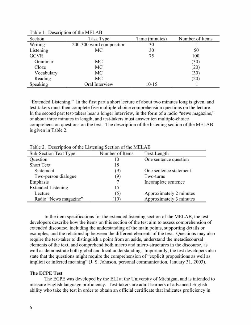
“Extended Listening.” In the first part a short lecture of about two minutes long is given, and test-takers must then complete five multiple-choice comprehension questions on the lecture. In the second part test-takers hear a longer interview, in the form of a radio “news magazine,” of about three minutes in length, and test-takers must answer ten multiple-choice comprehension questions on the text. The description of the listening section of the MELAB is given in Table 2.

Table 2. Description of the Listening Section of the MELAB Sub-Section Text Type Number of Items Text Length Question 10 One sentence question Short Text 18 Statement (9) One sentence statement Two-person dialogue (9) Two-turns Emphasis 7 Incomplete sentence Extended Listening 15 Lecture (5) Approximately 2 minutes Radio “News magazine” (10) Approximately 3 minutes

In the item specifications for the extended listening section of the MELAB, the test developers describe how the items on this section of the test aim to assess comprehension of extended discourse, including the understanding of the main points, supporting details or examples, and the relationship between the different elements of the text. Questions may also require the test-taker to distinguish a point from an aside, understand the metadiscoursal elements of the text, and comprehend both macro and micro-structures in the discourse, as well as demonstrate both global and local understanding. Importantly, the test developers also state that the questions might require the comprehension of “explicit propositions as well as implicit or inferred meaning” (J. S. Johnson, personal communication, January 31, 2003). The ECPE Test

The ECPE was developed by the ELI at the University of Michigan, and is intended to measure English language proficiency. Test-takers are adult learners of advanced English ability who take the test in order to obtain an official certificate that indicates proficiency in

7

English for use in the examinee's home country. Test-takers have approximately 155 minutes to complete the five sections of the test: speaking; written composition; listening comprehension; reading/cloze; and grammar/vocabulary/reading. The description of the test can be seen in Table 3.

Table 3. Description of the ECPE Section Task Type Time (minutes) Number of Items Speaking Oral Interview 10-15 1 Writing 200-300 word composition 30 1 Listening MC 25-30 40 Reading/Cloze MC cloze 25 40 GVR 60 100 Grammar MC (40) Vocabulary MC (40) Reading MC (20)

Extended Listening Section of the ECPE

The listening section of the ECPE is composed of three different sub-sections. In the first sub-section (17 items), the test-taker hears a question, and has to choose the best answer to that question. The second sub-section (13 items) has two different types of texts. With the first text type, the speaker hears a very short conversation of either two or three turns, and the test-taker has to choose the answer that means about the same thing as the statement or conversation that was presented. The second type of text in this section is a longer two-person conversation. For the 1999 administration, this text has seventeen turns, and five comprehension questions. The text is broken up into two parts. The first part is presented, then two comprehension questions are given. The text then continues, and three comprehension questions are given. The third sub-section of the listening section (10 items) involves longer texts. Although in these texts there is more than one speaker, it is not an interactive conversation. Rather, they are presented as a radio program, in which more than one speaker presents the information. Each of these texts has five multiple-choice comprehension items connected with it. The description of the listening section of the ECPE is given in Table 4. For the purpose of this study, the “Extended two-person dialogue” and the “Radio News magazine” text will be considered “extended listening.” Table 4. Description of the Listening Section of the ECPE Sub-Section Text Type Number of Items Text Length Question 17 One sentence question Conversation Two-person dialogue 8 Two or three turns Extended two-person dialogue 5 Approximately 20 turns Radio “News magazine” 10 Text 1 (5) Approximately 3 minutes Text 2 (5) Approximately 3 minutes

8

No item specifications were available for the ECPE, but it is assumed that since the extended listening sections of the ECPE are similar to the extended listening section of the MELAB, the item specifications described earlier for the MELAB would also apply to the ECPE.

Procedures MELAB

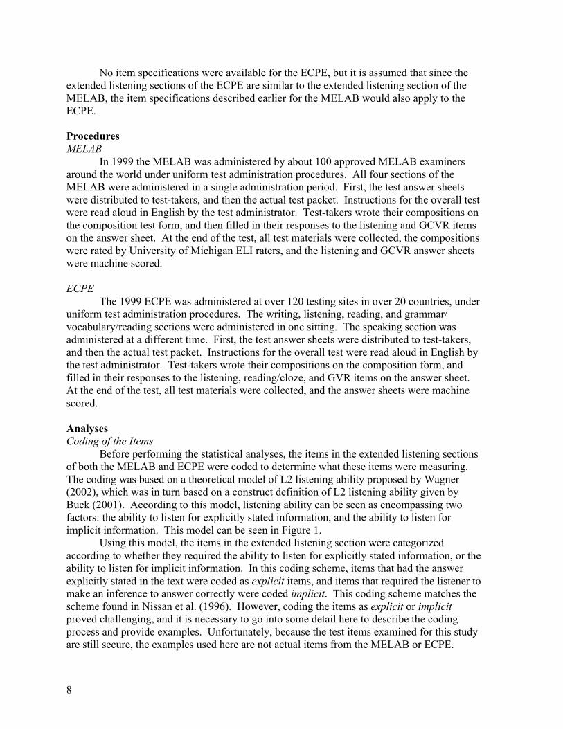
In 1999 the MELAB was administered by about 100 approved MELAB examiners around the world under uniform test administration procedures. All four sections of the MELAB were administered in a single administration period. First, the test answer sheets were distributed to test-takers, and then the actual test packet. Instructions for the overall test were read aloud in English by the test administrator. Test-takers wrote their compositions on the composition test form, and then filled in their responses to the listening and GCVR items on the answer sheet. At the end of the test, all test materials were collected, the compositions were rated by University of Michigan ELI raters, and the listening and GCVR answer sheets were machine scored. ECPE

The 1999 ECPE was administered at over 120 testing sites in over 20 countries, under uniform test administration procedures. The writing, listening, reading, and grammar/ vocabulary/reading sections were administered in one sitting. The speaking section was administered at a different time. First, the test answer sheets were distributed to test-takers, and then the actual test packet. Instructions for the overall test were read aloud in English by the test administrator. Test-takers wrote their compositions on the composition form, and filled in their responses to the listening, reading/cloze, and GVR items on the answer sheet. At the end of the test, all test materials were collected, and the answer sheets were machine scored.

Analyses Coding of the Items

Before performing the statistical analyses, the items in the extended listening sections of both the MELAB and ECPE were coded to determine what these items were measuring. The coding was based on a theoretical model of L2 listening ability proposed by Wagner (2002), which was in turn based on a construct definition of L2 listening ability given by Buck (2001). According to this model, listening ability can be seen as encompassing two factors: the ability to listen for explicitly stated information, and the ability to listen for implicit information. This model can be seen in Figure 1.

Using this model, the items in the extended listening section were categorized according to whether they required the ability to listen for explicitly stated information, or the ability to listen for implicit information. In this coding scheme, items that had the answer explicitly stated in the text were coded as explicit items, and items that required the listener to make an inference to answer correctly were coded implicit. This coding scheme matches the scheme found in Nissan et al. (1996). However, coding the items as explicit or implicit proved challenging, and it is necessary to go into some detail here to describe the coding process and provide examples. Unfortunately, because the test items examined for this study are still secure, the examples used here are not actual items from the MELAB or ECPE.

9

Figure 1. Operationalization of a Model of Second Language Listening Ability

An item coded explicit is one in which the answer to the item is explicitly stated in the text. The following item is an example:

The striped skunk is the most common type of skunk found in North America. Skunks are omnivorous mammals, about 2 feet in length. Q: A skunk is a type of _____. a. bird b. insect c. reptile d. mammal*

The correct answer, mammal, is explicitly stated in the text, and thus is coded explicit. The next example item coded explicit is less obvious:

And humans have also benefited from the presence of skunks, because skunks eat bugs like grasshoppers and insect larvae that often eat human agricultural crops. Q: Grasshoppers and larvae are examples of _____. a. different types of skunks b. agricultural pests that skunks eat* c. chemicals that cause a skunk’s odor d. predators that sometimes eat skunks

While the exact wording of the correct answer, agricultural pests that skunks eat, is not explicitly stated word for word in the text, the information found in the text (skunks eat bugs like grasshoppers and insect larvae…) is a close paraphrase or rewording of the correct answer, and thus is coded explicit. This idea of a “close paraphrase” will be examined more thoroughly after describing the coding of the implicit items.

Much of the research on listening for implicit information and making inferences in the L2 literature is based on the definitions of inferences given by Hildyard and Olson (1978).2 They described three different types of inferences that listeners must make: propositional inferences, enabling inferences, and pragmatic inferences. Propositional 2 In their study, Hildyard and Olson (1978) were describing the types of inferences that readers and listeners have to make.

Items measuring comprehension of implicit spoken information

Items measuring comprehension of explicitly stated spoken information L2 Listening

Ability

10

inferences are “those which are the necessary implications of explicit propositions” (Hildyard & Olson, 1978, p. 92), and include transitive relations or syllogisms, and comparative terms. Examples of this type of inference include the syllogism:

A is bigger than B. B is bigger than C. A is bigger than C. (Propositional inference)

Another example includes the use of comparative terms:

Alex has more than Deb. Deb has less than Alex. (Propositional inference)

Other types of propositional inferences according to Hildyard and Olson (1978) include the use of implicative verbs, and class inclusion relations. According to them, what all of these different types of propositional inferences have in common is that the inference follows from the form of the argument rather than from the content of the text.

A multiple-choice listening test item example might help to illustrate the idea of propositional inferences:

There are probably more skunks alive today than there were a thousand years ago. This is mostly because human development usually involves clearing the land of tree cover. This is fortunate for skunks, because they like to live in open areas. Q: According to the speaker, skunks have _____. a. been raised by humans as pets b. evolved in the last thousand years c. benefited from the presence of humans* d. almost gone extinct because of human development

This example can be seen as a type of syllogism. The listener hears, “Human development usually involves clearing the land of tree cover.” The listener also hears “Skunks like to live in open areas.” From these statements, the listener is able to make the inference “Skunks have benefited from human development,” which is a close paraphrase of the correct answer choice. It is important to note that with the propositional inference the listener does not need to utilize his or her world knowledge. Instead, the inference is a necessary implication drawn from the explicitly stated proposition. The inference is made from the form of the argument, rather than the content of that argument.

In contrast to propositional inferences, enabling inferences are those that allow the listener to link otherwise separate concepts in the text. They are made not as a result of an explicit, verbal proposition, but instead are made based on the listener’s knowledge of text structure (Hildyard & Olson, 1978), and these enabling inferences allow the listener to make sense out of the spoken utterances. Hildyard and Olson use the following example to illustrate (p. 94):

a. John threw the ball through the window. b. Mr. Jones came running out of the house. c. John broke the window (Enabling inference)

11

The listener’s world knowledge (that a ball can break a window, and that the owner of the house would be angry and would try to find the person responsible), and knowledge of the structure of spoken texts (that lines a and b are somehow related, and not independent) allow the listener to make the enabling inference that John had broken the window. Another multiple-choice item is given below as an example of an enabling inference:

A skunk’s odor works as a very good defense against predators. Skunks spray their musk at predators, causing a really bad smell. Q: Why is the skunk’s smell a good defense against predators? a. The predators can smell the skunks. b. Skunks use their odor to blend in to their environment. c. Skunks do not taste very good to predators because their odor is so bad. d. The predators know that if they attack the skunks, they will end up smelling

very bad.* The listener is forced to rely on his or her world knowledge to make the enabling inference required to answer the question correctly. The listener hears:

a. Skunks spray their musk at predators b. This causes a really bad smell.

From what he or she hears, the listener is able to make the following (rather extended) enabling inference to answer the question correctly:

c. The predators will end up smelling very bad if they attack the skunk. These predators will not want to smell bad, so they don’t attack skunks. Therefore, this is a good defense mechanism for the skunk.

Unlike propositional inferences, which are more or less independent of the content of the text, enabling inferences are made by listeners based on both the content and the structure of the spoken language (Hildyard & Olson, 1978).

The third type of inference described by Hildyard and Olson (1978) are pragmatic inferences. Like enabling inferences, they are made based on the listener’s world knowledge, but unlike enabling inferences, they are not essential for interpreting the basic content of the spoken text. Instead, they elaborate on the information given in the text, and allow the listener to make more subjective interpretations, based on the listener’s set of expectations about people, customs, and human behavior.

The three types of inferences described here all require the listener to utilize different knowledge sources. Hildyard and Olson (1978) summarize the three different types of inferences with the following:

Propositional inferences are the necessarily true implications of explicit propositions. Enabling inferences are inferences which must be drawn to make discourse coherent and therefore, comprehensible. Pragmatic inferences are probably true, nonessential elaborative inferences. (p. 95)

12

Using the theoretical model given above, instructions about how to code items, as well as examples of explicit and implicit coded items, four doctoral students in the Applied Linguistics program at Teachers College, Columbia University, were asked to code the 30 items examined here. Of the 30 items coded, only seven of the ECPE items were coded similarly by all four of the coders, and nine of the MELAB items were coded similarly by the four coders. In addition to these 16 items that all four coders agreed on, six of the ECPE items were coded similarly by three of the four coders, and five of the MELAB items were coded similarly by three of the four coders. With these 11 items, the researcher closely examined the items in question, and in 10 of the cases it was decided to code the items as the majority had coded them. Two of the ECPE items had an even split, with two of the coders coding them explicit, and the other two coding them implicit. Similarly, one of the MELAB items had an even split of coders. The results of the coding can be seen in Table 5. Table 5. Coding of the 30 MELAB and ECPE items Item

Initial Coding (4 raters)

Final Coding

Item

Initial Coding (4 raters)

Final Coding

MELAB 36 E E ECPE 26 I/E I MELAB 37 I I ECPE 27 I/E E MELAB 38 I/E I/E ECPE 28 I/E E MELAB 39 E E ECPE 29 I/E E MELAB 40 I/E I ECPE 30 I I MELAB 41 I/E I ECPE 31 E E MELAB 42 E E ECPE 32 E E MELAB 43 E E ECPE 33 I/E I/E MELAB 44 I I ECPE 34 I/E E MELAB 45 I/E I/E ECPE 35 I/E I MELAB 46 I I ECPE 36 E E MELAB 47 I/E E ECPE 37 I I MELAB 48 I/E E ECPE 38 I/E E MELAB 49 E E ECPE 39 I/E I/E MELAB 50 E E ECPE 40 I/E I Totals Explicit Implicit Implicit/Explicit MELAB 8 5 2 ECPE 8 5 2

The coding of the items was more difficult than anticipated, as is evidenced by the large number of disagreements between the coders. Part of this was due to the vagueness of the definitions in the literature. Deciding when an answer was implicit in the text, or if “a close paraphrase” (Nissan et al., 1996) was provided, proved difficult. Because of this, it was decided to code items 38 and 45 of the MELAB, and items 33 and 39 of the ECPE as double-coded, and to keep this double-coding in mind when examining how these items loaded on the particular factors.

13

Descriptive Statistics Descriptive statistics for each of the test items in the listening sections of the MELAB

and the ECPE were calculated and assumptions of normality were analyzed using SPSS version 10.0.5 for the PC. First, the mean, median, and standard deviation for each of the items were calculated, in order to examine the central tendencies and variability of the responses. This was done so that the appropriateness of each item in the assessments could be considered. Items with extreme means would indicate that these items might be too easy or too difficult for this population of students, and might not be suitable for the analysis. To check if the items were normally distributed, the skewness and kurtosis for each of the items were analyzed. Because the statistical analyses employed in this study assumed a normal distribution, if an item had extreme skewness or kurtosis, it was considered for deletion from further analyses.

Reliability Analysis

A series of internal consistency reliability estimates for the overall listening sections of the MELAB (50 items) and the ECPE (40 items) using Cronbach’s alpha were computed. All of these calculations were computed using SPSS version 10.0.5 for the PC. The internal consistency reliability estimates were also calculated for each of the sub-sections (including the extended listening sub-section) of the listening sections of the MELAB and the ECPE, again using Cronbach’s alpha.

For the extended listening sections (composed of 15 items for each of the tests), item-total correlations were also computed. This was done in order to investigate how each individual item performed in relation to the other items in the extended listening sections. Those items that performed poorly were examined in order to determine if they should be considered for deletion from further analysis.

Exploratory Factor Analysis

After the items were coded, a number of exploratory factor analyses (EFAs) were performed in an attempt to examine the patterns of correlations among the items in order to explore the basic underlying factors of the extended listening sections of the tests. For this study, it was theorized that the factor analysis for each of the tests would result in a two-factor solution: one factor would correspond to the ability to listen for explicitly stated information, and the second factor would correspond to the ability to listen for implicit information. The items that were coded explicit should have loaded on a factor corresponding to the ability to listen for explicitly stated information, and the items that were coded implicit should have loaded on a factor corresponding to the ability to listen for implicit information.

The data from the extended listening sections of both of the tests were based on answers scored dichotomously, and thus the variables were treated as categorical. As a result, tetrachoric correlations were required in performing the EFAs. These EFAs were performed using Mplus for Windows, version 2.02, which computes tetrachoric correlations. First, the correlation matrix was prepared, and the determinant of the matrix was examined to determine the appropriateness of the data for factor analysis.

The EFAs were then performed, using unweighted least squares analysis (which is an appropriate analysis to use with categorical data) to extract the initial factors. The eigenvalues and the scree plots for the two sections were examined as indicators of the number of factors represented by the data, and then this information was used in an attempt to

14

determine if the underlying factors represented by the data were consistent with the theoretical construct described earlier. Another EFA was then performed, using unweighted least squares analysis with a Varimax rotation to obtain an orthogonal solution, and a Promax rotation to obtain an oblique solution. To determine which rotation procedure was most appropriate for these data, the interfactor correlation matrices were examined, and meaningful interpretations were made as the final criteria for deciding the best number of factors to extract.

Results

MELAB Descriptive Statistics

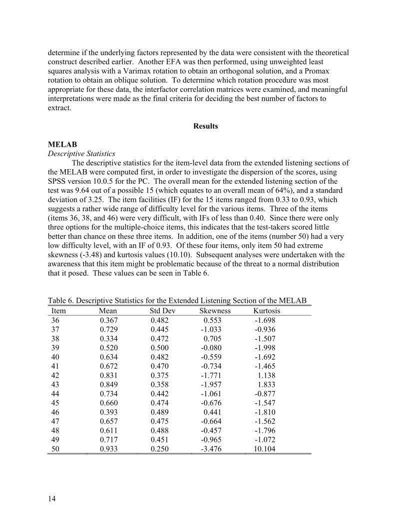
The descriptive statistics for the item-level data from the extended listening sections of the MELAB were computed first, in order to investigate the dispersion of the scores, using SPSS version 10.0.5 for the PC. The overall mean for the extended listening section of the test was 9.64 out of a possible 15 (which equates to an overall mean of 64%), and a standard deviation of 3.25. The item facilities (IF) for the 15 items ranged from 0.33 to 0.93, which suggests a rather wide range of difficulty level for the various items. Three of the items (items 36, 38, and 46) were very difficult, with IFs of less than 0.40. Since there were only three options for the multiple-choice items, this indicates that the test-takers scored little better than chance on these three items. In addition, one of the items (number 50) had a very low difficulty level, with an IF of 0.93. Of these four items, only item 50 had extreme skewness (-3.48) and kurtosis values (10.10). Subsequent analyses were undertaken with the awareness that this item might be problematic because of the threat to a normal distribution that it posed. These values can be seen in Table 6. Table 6. Descriptive Statistics for the Extended Listening Section of the MELAB Item Mean Std Dev Skewness Kurtosis 36 0.367 0.482 0.553 -1.698 37 0.729 0.445 -1.033 -0.936 38 0.334 0.472 0.705 -1.507 39 0.520 0.500 -0.080 -1.998 40 0.634 0.482 -0.559 -1.692 41 0.672 0.470 -0.734 -1.465 42 0.831 0.375 -1.771 1.138 43 0.849 0.358 -1.957 1.833 44 0.734 0.442 -1.061 -0.877 45 0.660 0.474 -0.676 -1.547 46 0.393 0.489 0.441 -1.810 47 0.657 0.475 -0.664 -1.562 48 0.611 0.488 -0.457 -1.796 49 0.717 0.451 -0.965 -1.072 50 0.933 0.250 -3.476 10.104

15

Internal Consistency Reliability An internal consistency reliability analysis was performed on the 50-item listening

section of the MELAB, in order to examine how each listening item correlated with the other listening items. The internal consistency reliability for the overall listening section was high (a = 0.901).

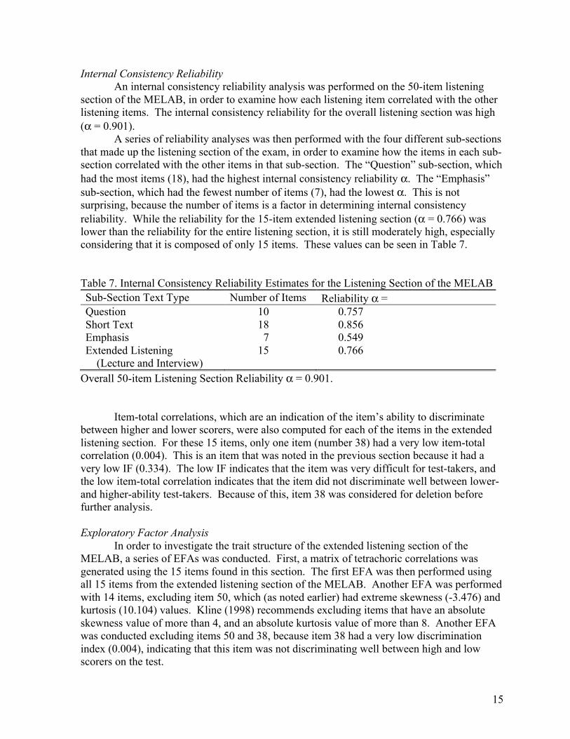
A series of reliability analyses was then performed with the four different sub-sections that made up the listening section of the exam, in order to examine how the items in each sub-section correlated with the other items in that sub-section. The “Question” sub-section, which had the most items (18), had the highest internal consistency reliability a. The “Emphasis” sub-section, which had the fewest number of items (7), had the lowest a. This is not surprising, because the number of items is a factor in determining internal consistency reliability. While the reliability for the 15-item extended listening section (a = 0.766) was lower than the reliability for the entire listening section, it is still moderately high, especially considering that it is composed of only 15 items. These values can be seen in Table 7.

Table 7. Internal Consistency Reliability Estimates for the Listening Section of the MELAB Sub-Section Text Type Number of Items Reliability a = Question 10 0.757 Short Text 18 0.856 Emphasis 7 0.549 Extended Listening 15 0.766 (Lecture and Interview)

Overall 50-item Listening Section Reliability a = 0.901.

Item-total correlations, which are an indication of the item’s ability to discriminate between higher and lower scorers, were also computed for each of the items in the extended listening section. For these 15 items, only one item (number 38) had a very low item-total correlation (0.004). This is an item that was noted in the previous section because it had a very low IF (0.334). The low IF indicates that the item was very difficult for test-takers, and the low item-total correlation indicates that the item did not discriminate well between lower- and higher-ability test-takers. Because of this, item 38 was considered for deletion before further analysis.

Exploratory Factor Analysis

In order to investigate the trait structure of the extended listening section of the MELAB, a series of EFAs was conducted. First, a matrix of tetrachoric correlations was generated using the 15 items found in this section. The first EFA was then performed using all 15 items from the extended listening section of the MELAB. Another EFA was performed with 14 items, excluding item 50, which (as noted earlier) had extreme skewness (-3.476) and kurtosis (10.104) values. Kline (1998) recommends excluding items that have an absolute skewness value of more than 4, and an absolute kurtosis value of more than 8. Another EFA was conducted excluding items 50 and 38, because item 38 had a very low discrimination index (0.004), indicating that this item was not discriminating well between high and low scorers on the test.

16

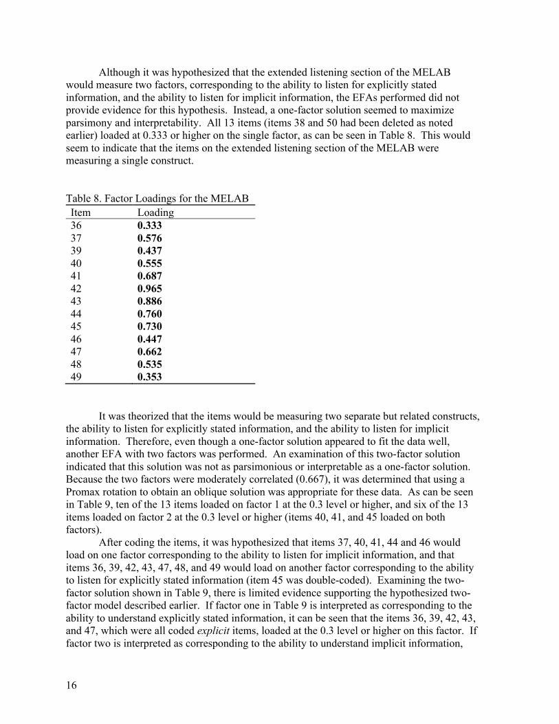
Although it was hypothesized that the extended listening section of the MELAB would measure two factors, corresponding to the ability to listen for explicitly stated information, and the ability to listen for implicit information, the EFAs performed did not provide evidence for this hypothesis. Instead, a one-factor solution seemed to maximize parsimony and interpretability. All 13 items (items 38 and 50 had been deleted as noted earlier) loaded at 0.333 or higher on the single factor, as can be seen in Table 8. This would seem to indicate that the items on the extended listening section of the MELAB were measuring a single construct.

Table 8. Factor Loadings for the MELAB Item Loading 36 0.333 37 0.576 39 0.437 40 0.555 41 0.687 42 0.965 43 0.886 44 0.760 45 0.730 46 0.447 47 0.662 48 0.535 49 0.353

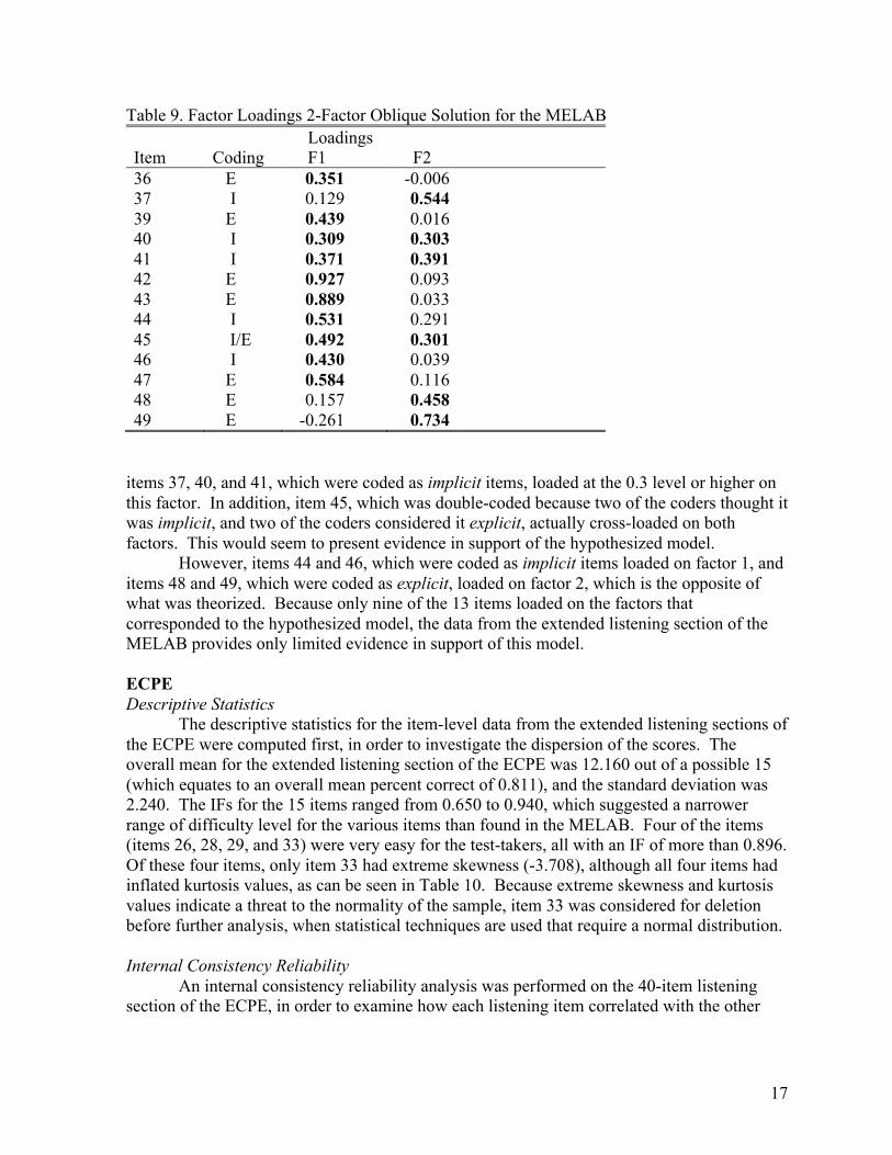
It was theorized that the items would be measuring two separate but related constructs, the ability to listen for explicitly stated information, and the ability to listen for implicit information. Therefore, even though a one-factor solution appeared to fit the data well, another EFA with two factors was performed. An examination of this two-factor solution indicated that this solution was not as parsimonious or interpretable as a one-factor solution. Because the two factors were moderately correlated (0.667), it was determined that using a Promax rotation to obtain an oblique solution was appropriate for these data. As can be seen in Table 9, ten of the 13 items loaded on factor 1 at the 0.3 level or higher, and six of the 13 items loaded on factor 2 at the 0.3 level or higher (items 40, 41, and 45 loaded on both factors).

After coding the items, it was hypothesized that items 37, 40, 41, 44 and 46 would load on one factor corresponding to the ability to listen for implicit information, and that items 36, 39, 42, 43, 47, 48, and 49 would load on another factor corresponding to the ability to listen for explicitly stated information (item 45 was double-coded). Examining the two-factor solution shown in Table 9, there is limited evidence supporting the hypothesized two-factor model described earlier. If factor one in Table 9 is interpreted as corresponding to the ability to understand explicitly stated information, it can be seen that the items 36, 39, 42, 43, and 47, which were all coded explicit items, loaded at the 0.3 level or higher on this factor. If factor two is interpreted as corresponding to the ability to understand implicit information,

17

Table 9. Factor Loadings 2-Factor Oblique Solution for the MELAB Loadings Item Coding F1 F2 36 E 0.351 -0.006 37 I 0.129 0.544 39 E 0.439 0.016 40 I 0.309 0.303 41 I 0.371 0.391 42 E 0.927 0.093 43 E 0.889 0.033 44 I 0.531 0.291 45 I/E 0.492 0.301 46 I 0.430 0.039 47 E 0.584 0.116 48 E 0.157 0.458 49 E -0.261 0.734

items 37, 40, and 41, which were coded as implicit items, loaded at the 0.3 level or higher on this factor. In addition, item 45, which was double-coded because two of the coders thought it was implicit, and two of the coders considered it explicit, actually cross-loaded on both factors. This would seem to present evidence in support of the hypothesized model.

However, items 44 and 46, which were coded as implicit items loaded on factor 1, and items 48 and 49, which were coded as explicit, loaded on factor 2, which is the opposite of what was theorized. Because only nine of the 13 items loaded on the factors that corresponded to the hypothesized model, the data from the extended listening section of the MELAB provides only limited evidence in support of this model.

ECPE Descriptive Statistics

The descriptive statistics for the item-level data from the extended listening sections of the ECPE were computed first, in order to investigate the dispersion of the scores. The overall mean for the extended listening section of the ECPE was 12.160 out of a possible 15 (which equates to an overall mean percent correct of 0.811), and the standard deviation was 2.240. The IFs for the 15 items ranged from 0.650 to 0.940, which suggested a narrower range of difficulty level for the various items than found in the MELAB. Four of the items (items 26, 28, 29, and 33) were very easy for the test-takers, all with an IF of more than 0.896. Of these four items, only item 33 had extreme skewness (-3.708), although all four items had inflated kurtosis values, as can be seen in Table 10. Because extreme skewness and kurtosis values indicate a threat to the normality of the sample, item 33 was considered for deletion before further analysis, when statistical techniques are used that require a normal distribution. Internal Consistency Reliability

An internal consistency reliability analysis was performed on the 40-item listening section of the ECPE, in order to examine how each listening item correlated with the other

18

Table 10. Descriptive Statistics for the Extended Listening Section of the ECPE Item Mean Std Dev Skewness Kurtosis 26 0.901 0.298 -2.691 5.241 27 0.871 0.335 -2.219 2.925 28 0.896 0.306 -2.587 4.692 29 0.911 0.285 -2.879 6.291 30 0.720 0.449 -0.981 -1.039 31 0.847 0.360 -1.931 1.727 32 0.830 0.376 -1.752 1.070 33 0.940 0.237 -3.708 11.750 34 0.825 0.380 -1.709 0.922 35 0.861 0.346 -2.083 2.338 36 0.697 0.460 -0.858 -1.264 37 0.723 0.447 -0.998 -1.004 38 0.650 0.477 -0.628 -1.606 39 0.777 0.416 -1.331 -0.228 40 0.712 0.453 -0.934 -1.264

listening items. The internal consistency reliability for the overall listening section was moderate (a = 0.768).

A series of reliability analyses was then performed with the three different sub-sections that made up the listening section of the exam, in order to examine how the items in each sub-section correlated with the other items in that sub-section. The “Extended Listening” sub-section had the highest internal consistency reliability a, even though it had two fewer items than the “Questions” sub-section. The “Conversation” sub-section, which had the fewest number of items (8), had the lowest a. Again, this is not surprising, because the number of items is a factor in determining internal consistency reliability. The reliability for the 15-item extended listening section (a = 0.605) was lower than the reliability for the entire listening section. These values can be seen in Table 11.

Table 11. Internal Consistency Reliability Estimates for the Listening Section of the ECPE Sub-section Text Type Number of Items Reliability a = Question 17 0.560 Conversation 8 0.539 Extended Listening3 15 0.605

Overall 40-item Listening Section Reliability a = 0.768.

Item-total correlations were also computed for each of the items in the extended listening section. For these 15 items, three items had an item-total correlation lower than 0.200. Item 33 had an item-total correlation of 0.169, item 37 had an item-total correlation of 0.168, and 3 For this analysis, the “Extended Listening” includes the “Extended two-person dialogue” sub-section, which on the test was part of the “Conversation” sub-section.

19

item 40 had an item-total correlation of 0.188. In addition, five items (28, 31, 32, 34, and 39) had item-total correlations ranging from 0.207 to 0.216. The relatively low item-total correlation values indicate that the items do not discriminate well between lower- and higher-ability test-takers, and also are responsible for the relatively low internal consistency reliability for the “Extended Listening” sub-section, and also contribute to the lower reliability for the overall listening section. Of these seven items with low item-total correlations, only items 28 and 33 were also flagged earlier for having inflated skewness and/or kurtosis values. These items had high IFs, (0.896 and 0.940, respectively), indicating that these items were relatively easy for the test-takers, which can probably account for the low item-total correlations. However, the other five items with low item-total correlations (31, 32, 37, 39, and 40) had lower IFs, ranging from 0.712 to 0.847.

Exploratory Factor Analysis

In order to investigate the trait structure of the extended listening section of the ECPE, a series of EFAs was conducted. First, a matrix of tetrachoric correlations was generated using the 15 items found in this section. The first EFA was then performed using all 15 items from the extended listening section of the ECPE. Another EFA was performed with 14 items, excluding item 33, which (as noted earlier) had extreme skewness (-3.708) and kurtosis (11.750) values.

Although it was hypothesized that the extended listening section of the ECPE would measure two factors, corresponding to the ability to listen for explicitly stated information and the ability to listen for implicit information, the EFAs performed did not provide evidence for this hypothesis. Instead, two possible solutions seemed to maximize parsimony and interpretability. Similar to the MELAB findings, a one-factor solution could be interpreted from the loadings on the EFA. Twelve of the 14 items loaded on factor 1 at a level of 0.3 or higher, and are shown in bold in Table 12. Only two of the items (37 and 40) loaded lower than 0.3 on the one-factor solution, although both of these items loaded on the factor at 0.233 or above. Table 12. Factor Loadings 1-Factor Solution for the ECPE Item Loading 26 0.755 27 0.686 28 0.474 29 0.668 30 0.518 31 0.393 32 0.348 34 0.372 35 0.420 36 0.436 37 0.233 38 0.355 39 0.324 40 0.282

20

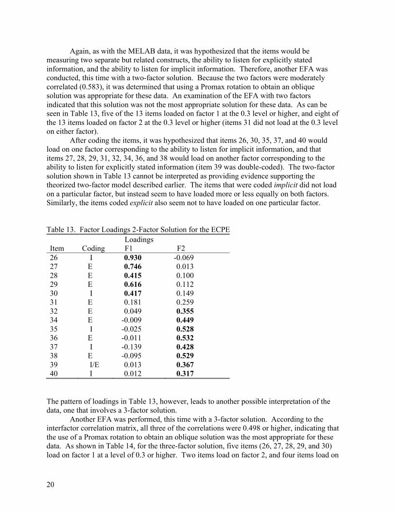
Again, as with the MELAB data, it was hypothesized that the items would be measuring two separate but related constructs, the ability to listen for explicitly stated information, and the ability to listen for implicit information. Therefore, another EFA was conducted, this time with a two-factor solution. Because the two factors were moderately correlated (0.583), it was determined that using a Promax rotation to obtain an oblique solution was appropriate for these data. An examination of the EFA with two factors indicated that this solution was not the most appropriate solution for these data. As can be seen in Table 13, five of the 13 items loaded on factor 1 at the 0.3 level or higher, and eight of the 13 items loaded on factor 2 at the 0.3 level or higher (items 31 did not load at the 0.3 level on either factor).

After coding the items, it was hypothesized that items 26, 30, 35, 37, and 40 would load on one factor corresponding to the ability to listen for implicit information, and that items 27, 28, 29, 31, 32, 34, 36, and 38 would load on another factor corresponding to the ability to listen for explicitly stated information (item 39 was double-coded). The two-factor solution shown in Table 13 cannot be interpreted as providing evidence supporting the theorized two-factor model described earlier. The items that were coded implicit did not load on a particular factor, but instead seem to have loaded more or less equally on both factors. Similarly, the items coded explicit also seem not to have loaded on one particular factor. Table 13. Factor Loadings 2-Factor Solution for the ECPE Loadings Item Coding F1 F2 26 I 0.930 -0.069 27 E 0.746 0.013 28 E 0.415 0.100 29 E 0.616 0.112 30 I 0.417 0.149 31 E 0.181 0.259 32 E 0.049 0.355 34 E -0.009 0.449 35 I -0.025 0.528 36 E -0.011 0.532 37 I -0.139 0.428 38 E -0.095 0.529 39 I/E 0.013 0.367 40 I 0.012 0.317

The pattern of loadings in Table 13, however, leads to another possible interpretation of the data, one that involves a 3-factor solution.

Another EFA was performed, this time with a 3-factor solution. According to the interfactor correlation matrix, all three of the correlations were 0.498 or higher, indicating that the use of a Promax rotation to obtain an oblique solution was the most appropriate for these data. As shown in Table 14, for the three-factor solution, five items (26, 27, 28, 29, and 30) load on factor 1 at a level of 0.3 or higher. Two items load on factor 2, and four items load on

21

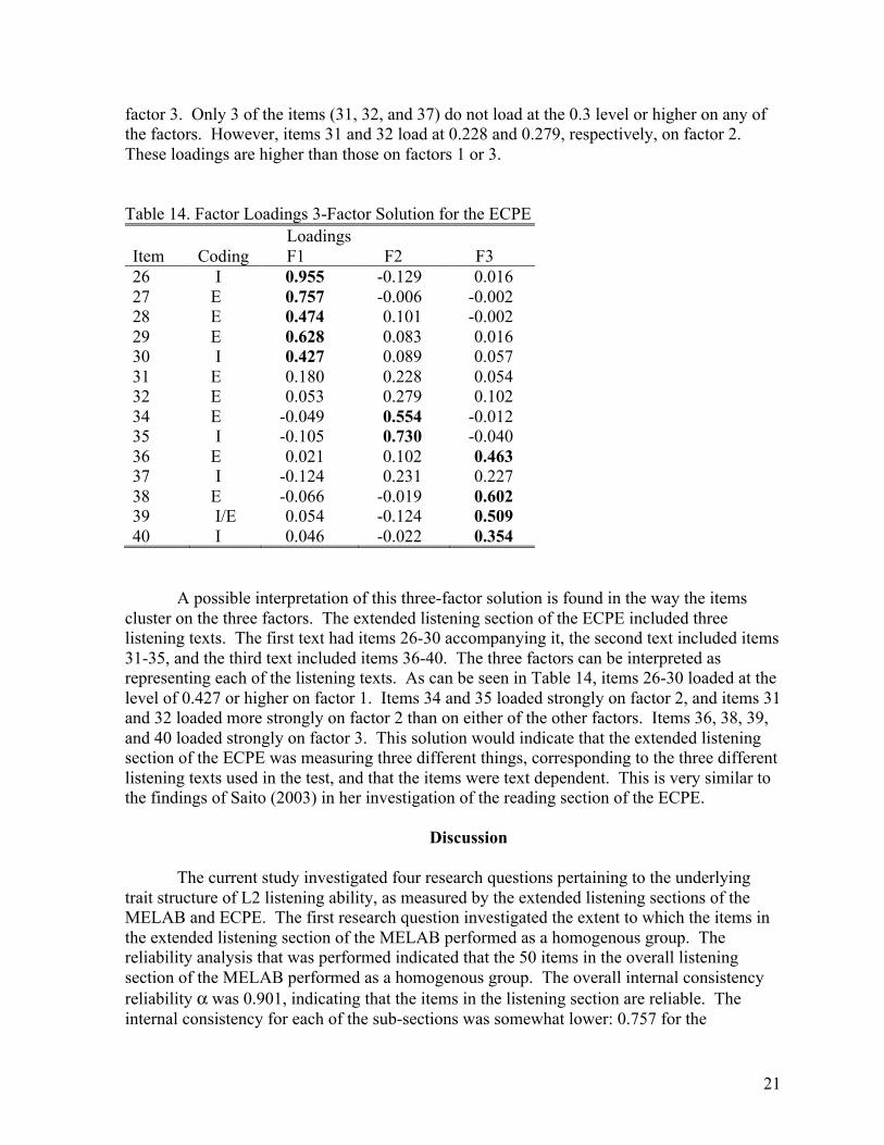
factor 3. Only 3 of the items (31, 32, and 37) do not load at the 0.3 level or higher on any of the factors. However, items 31 and 32 load at 0.228 and 0.279, respectively, on factor 2. These loadings are higher than those on factors 1 or 3.

Table 14. Factor Loadings 3-Factor Solution for the ECPE Loadings Item Coding F1 F2 F3 26 I 0.955 -0.129 0.016 27 E 0.757 -0.006 -0.002 28 E 0.474 0.101 -0.002 29 E 0.628 0.083 0.016 30 I 0.427 0.089 0.057 31 E 0.180 0.228 0.054 32 E 0.053 0.279 0.102 34 E -0.049 0.554 -0.012 35 I -0.105 0.730 -0.040 36 E 0.021 0.102 0.463 37 I -0.124 0.231 0.227 38 E -0.066 -0.019 0.602 39 I/E 0.054 -0.124 0.509 40 I 0.046 -0.022 0.354

A possible interpretation of this three-factor solution is found in the way the items cluster on the three factors. The extended listening section of the ECPE included three listening texts. The first text had items 26-30 accompanying it, the second text included items 31-35, and the third text included items 36-40. The three factors can be interpreted as representing each of the listening texts. As can be seen in Table 14, items 26-30 loaded at the level of 0.427 or higher on factor 1. Items 34 and 35 loaded strongly on factor 2, and items 31 and 32 loaded more strongly on factor 2 than on either of the other factors. Items 36, 38, 39, and 40 loaded strongly on factor 3. This solution would indicate that the extended listening section of the ECPE was measuring three different things, corresponding to the three different listening texts used in the test, and that the items were text dependent. This is very similar to the findings of Saito (2003) in her investigation of the reading section of the ECPE.

Discussion

The current study investigated four research questions pertaining to the underlying

trait structure of L2 listening ability, as measured by the extended listening sections of the MELAB and ECPE. The first research question investigated the extent to which the items in the extended listening section of the MELAB performed as a homogenous group. The reliability analysis that was performed indicated that the 50 items in the overall listening section of the MELAB performed as a homogenous group. The overall internal consistency reliability a was 0.901, indicating that the items in the listening section are reliable. The internal consistency for each of the sub-sections was somewhat lower: 0.757 for the

22

“Question” sub-section; 0.856 for the “Short Text” sub-section; 0.549 for the “Emphasis” sub-section; and 0.766 for the “Extended Listening” sub-section. This would seem to indicate that these items are measuring reliably the different components of the construct.

The second research question examined the underlying trait structure of the extended listening section of the MELAB. A model of L2 listening ability was hypothesized, and then EFA was used to investigate if the MELAB assessed test-takers’ ability to listen for explicitly stated information, and the ability to listen for implicit information. The two-factor oblique solution for the EFA that was performed seemed to present evidence in support of the hypothesized model. There seemed to be a meaningful pattern of variable loadings on the two factors: three of the five items coded implicit loaded on one factor; and five of the seven items coded explicit loaded on the other factor. In addition, the one item that was double-coded loaded on both factors. Still, four of the 13 items loaded on the opposite factor of what had been predicted.

The third research question investigated the extent to which the items in the extended listening section of the ECPE performed as a homogenous group. The reliability analysis that was performed indicated that the 40 items in the overall listening section of the ECPE performed as a fairly homogenous group. The overall internal consistency reliability a was 0.768, indicating that the items in the listening section are moderately reliable. The internal consistency measures for each of the sub-sections were somewhat lower: 0.560 for the “Question” sub-section; 0.539 for the “Conversation” sub-section; and 0.605 for the “Extended Listening” sub-section. This would seem to indicate that these items are measuring fairly reliably the different components of the construct. However, the internal consistency reliability a was markedly lower for the listening section of the ECPE than for the MELAB. Again, this may in part be due to the fact that the ECPE listening section (40 items) had ten fewer items than the MELAB listening section (50 items). It may also have to do with the fact that the sub-sections of the ECPE were somewhat different from the sub-sections of the MELAB. While both tests had a “Question” and “Extended Listening” sub-section, the ECPE also had a “Conversation” sub-section, while the MELAB had a “Short Text” and an “Emphasis” sub-section. It should also be noted that the “Question” sub-section of the ECPE had a much lower reliability a (0.560) for the ECPE compared with a 0.757 reliability a for this sub-section of the MELAB. Similarly, the a (0.605) for the “Extended Listening” section of the ECPE is lower than the reliability a (0.766) for the comparable section of the MELAB. Assuming that the item specifications for both of these tests were similar, investigating why the reliability of the corresponding sections of the two tests varied so markedly could be an informative area for further research.

The fourth research question examined the underlying trait structure of the extended listening section of the ECPE. A model of L2 listening ability was hypothesized, and then EFA was used to investigate if the ECPE assessed test-takers’ ability to listen for explicitly stated information, and the ability to listen for implicit information. The EFA that was performed, however, presented no evidence in support of the hypothesized two-factor model. Instead, a one-factor or a three-factor solution seemed more interpretable for the data. The one-factor solution would seem to indicate that the extended listening section of the ECPE was measuring a single construct. The three-factor solution seemed to indicate that the items were text dependent. For the most part, the items clustered together with the rest of the items that were measuring the same text, and each factor could be interpreted as corresponding to a particular text.

23

Although the analyses of the EFAs conducted on the data from the MELAB provided only limited evidence in support of the hypothesized model, and the data from the ECPE provided little evidence, there are many factors that might explain at least some of the lack of supporting evidence. Firstly, the measures of reliability for the extended listening sections of the test were relatively low, at 0.766 for the MELAB, and 0.605 for the ECPE. Again, this is at least in part due to the small number of items (15) in these sections. Regardless of the cause, this amount of random measurement error makes it more difficult when using factor analysis to find evidence for the hypothesized model. Also, the fact that the items in the ECPE appeared to be text dependent is another factor that probably had an effect on the results of the EFA, and the investigation of this apparent text dependency could be an area in which further research might be fruitful.

Secondly, the coding of the items was a problematic process, and even though efforts were made to systematize the coding system, the process still included a degree of personal subjectivity. Although this is probably an inevitable part of any coding process, part of this inherent subjectivity could be due to the fine gradations of definitions of what making an inference actually entails. The definitions for the coding were based largely on Hildyard and Olson’s (1978) work, in which the definitions of the three different types of inferences are thoroughly delineated, and numerous examples were given, and yet implementing these definitions in the coding process was still challenging, especially when trying to differentiate between an inference and a close paraphrase, as Nissan et al. (1996) described it. Also, the items from these tests were not operationalized on this model of listening ability. Instead, this model had been imposed on the items, and thus contributes to the difficulty of the coding process.

Thirdly, the distinction between the ability to listen for explicitly stated information and implicit information is at least to some extent an artificial one. Listeners still must be able to understand the explicitly stated words or phrases that will allow them to make the inference necessary to understand the implied information. At least on some levels, the ability to listen for implicit information cannot be separated from the ability to listen for explicitly stated information. The relatively high correlation (0.667) between the two factors in the two-factor solution of the MELAB may be an indication of how the two abilities might not be able to be truly separated. It may be that it is necessary for the listener to be listening for both explicitly stated and implicit information simultaneously, and trying to separate the two is an artificial division. Even with the difficulties mentioned above, there was some evidence supporting the hypothesized model found in the data from the EFA performed with the data from the extended listening section of the MELAB.

It must also be kept in mind that this study looked specifically at the extended listening sections of the tests. However, the listening section of the MELAB also had three other sub-sections (“Questions”, “Short Text” and “Emphasis”), and the ECPE listening section had two other sub-sections (“Questions” and “Conversation”) that were intended to test different aspects of the L2 listening process. Shin (2003) investigated the construct validity of the “Emphasis” sub-section of the MELAB, and further studies of this nature investigating the various sub-sections of the test would be useful and informative.

24

Conclusion

Buck (2001) urged that the taxonomies found in the L2 listening literature be treated with caution, because they were based on theory only, and had not been empirically validated. He also stated that there was an unspoken assumption that the sub-skills given in the taxonomies were in fact skills, and that the “research seems to suggest that we are able to identify them statistically at almost any level of detail” (p. 59). This study was an attempt to empirically validate a more general model of L2 listening ability, one that includes the ability to listen for explicitly stated information, and the ability to listen for implicit information. The results of the study mirror Buck’s warning, that identifying statistically the different abilities involved in L2 listening is not an easy task. While only limited evidence was found here in support of the hypothesized model, the proposed model warrants further research in an attempt to allow L2 listening test developers to make more reliable and valid assessments.

References

Aitken, K. (1978). Measuring listening comprehension. English as a Second Language. TEAL

Occasional Papers, 2. Vancouver: British Colombia Association of Teachers of English as an Additional Language. (ERIC Document Reproduction Service, No. ED 155 945)

Brindley, G. (1998). Assessing listening abilities. Annual Review of Applied Linguistics, 18, 171-191.

Buck, G. (1991) The test of listening comprehension: An introspective study. Language Testing, 8(1), 67-91.

Buck, G. (2001). Assessing listening. Cambridge: Cambridge University Press. Buck, G., & Tatsuoka, K. (1998). Application of the rule-space procedure to language testing:

Examining attributes of a free response listening test. Language Testing, 15(2), 119-157. Dunkel, P., Henning, G., & Chaudron, C. (1993). The assessment of an L2 listening

comprehension construct: A tentative model for test specification and development. Modern Language Journal, 77(2), 180-91.

Hansen, C., & Jensen, C. (1994). Evaluating lecture comprehension. In J. Flowerdew (Ed.), Academic listening (pp. 241-268). New York: Cambridge University Press.

Hildyard, A., & Olson, D. (1978). Memory and inference in the comprehension of oral and written discourse. Discourse Processes, 1(1), 91-107.

Kline, R. (1998). Principles and practice of structural equation modeling. New York: The Guilford Press.

Lund, R. (1991). A comparison of second language listening and reading comprehension. Modern Language Journal, 75(2), 196-204.

Nissan, S., Devnicenzi, F., & Tang, K. (1996). An analysis of factors affecting the difficulty of dialogue items in TOEFL listening comprehension (TOEFL Research Report No. 51). Princeton, NJ: Educational Testing Service.

Peterson, P. (1991). A synthesis of methods for interactive listening. In M. Celce-Murcia (Ed.), Teaching English as a second or foreign language (2nd ed.) (pp. 106-122). New York: Newbury House.

Purpura, J. (1999). Learner strategy use and performance on language tests: A structural equation modeling approach. Cambridge: Cambridge University Press.

25

Richards, J. (1983). Listening comprehension: Approach, design, procedure. TESOL Quarterly, 17(2), 219-40.

Rost, M. (1990). Listening in language learning. New York: Longman. Rubin, J. (1994). A review of second language listening comprehension research. Modern

Language Journal, 78(2), 199-221. Saito, Y. (2003). Investigating the construct validity of the cloze section in the Examination

for the Certificate of Proficiency in English. Spaan Fellow Working Papers in Second or Foreign Language Assessment, 1, 39-82. Ann Arbor, MI: University of Michigan English Language Institute.

Shin, S. (2003). A construct validation study of emphasis type questions in the Michigan English Language Assessment Battery. Spaan Fellow Working Papers in Second or Foreign Language Assessment, 1, 25-37. Ann Arbor, MI: University of Michigan English Language Institute.

Wagner, E. (2002). Video listening tests: A pilot study. Working Papers in TESOL & Applied Linguistics, Teachers College, Columbia University, 2/1, Retrieved March 31, 2003, from http://www.tc.edu/tesolalwebjournal/wagner.pdf.

Weir, C. (1993). Understanding and developing language tests. Hemel Hempstead: Prentice-Hall.

26

Spaan Fellow Working Papers in Second or Foreign Language Assessment 27 Volume 2, 2004 English Language Institute, University of Michigan

Evaluating the Dimensionality of the Michigan English Language Assessment Battery

Hong Jiao

Florida State University

This study evaluates the dimensionality of Form FF, listening and Form EE, grammar/cloze/vocabulary/reading (GCVR) in the Michigan English Language Assessment Battery (MELAB). It further investigates the influences of gender, native language, and proficiency level on the dimensionality of the listening and the GCVR sections in the MELAB. Stout’s procedure was employed to test two hypotheses; that the listening items are unidimensional, and the GCVR items are unidimensional. Principle axes factor analysis and principle component analysis both using the tetrachoric correlation matrix were applied for further exploration. The results indicate that both listening and GCVR tests were unidimensional for female and Tagalog/Filipino-speaking groups. Further, the global GCVR test was unidimensional. But for other groups, the results were inconsistent across methods regarding the unidimensionality of both forms.

Validity is an important issue in test development and evaluation according to the Standards for Educational and Psychological Testing (American Educational Research Association, American Psychological Association, & National Council on Measurement in Education, 1999), as well as fairness. Validity refers to the degree to which evidence supports the inferences based on test scores (Messick, 1989). Fairness means that all examinees are given comparable opportunities to demonstrate their abilities on the construct a test intends to measure (American Educational Research Association, et al., 1999, p.74). In examining test fairness, the researcher should address questions such as whether the test measures the same construct in all relevant populations (Wang & Witt, 2002). An investigation of the factor structure of a test can provide evidence of validity (Messick, 1995) and fairness of the test.

To make valid and fair comparisons across examinee groups, test items should be constructed to measure the same construct(s). However, test items often measure other traits in addition to the traits they intend to measure (Hambleton & Swaminathan, 1985; Reckase, 1979, 1985; Stout, 1987). Several studies (Birenbaum & Tatsuoka, 1982; Bock, Gibbons, & Muraki, 1988) indicated that item attributes and examinee characteristics could affect the dimensionality of test items. Dimensionality is a property of the test as well as of the examinees (Reckase, 1990). This is also true with language proficiency tests. Oltman and Stricker (1988) and Kok (1992) showed that examinees’ English proficiency and ethnic background affected the dimensionality of language proficiency tests. Therefore, when evaluating the dimensionality of a test, it would provide a better picture if the evaluation were done from the perspective of both the test itself and the examinees’ characteristics.

The Michigan English Language Assessment Battery (MELAB) is a test developed for college and university admission. It intends to assess the English language competence of adult non-native speakers of English who will apply to study at an English-speaking institution. The MELAB includes Part 1, writing on a prompt, Part 2, a listening

28

comprehension test, Part 3, grammar, cloze, vocabulary, and reading comprehension (GCVR) questions, and an optional speaking test. All the items in the listening and GCVR subtests are scored dichotomously.

The MELAB Technical Manual (English Language Institute, University of Michigan, 1996) reported factor analysis results, done at the component score level, of Part 2 and Part 3 in the MELAB. The Michigan English Language Assessment Battery: Technical Manual 2003 (English Language Institute, University of Michigan, 2003) reported an item factor analysis of the individual items in Part 2 and Part 3 sections of the MELAB, and principle component analysis of the testlet scores. The item-level factor analysis provided more information regarding the construct validity of Part 2 and Part 3 in the MELAB.

The purpose of this study is to evaluate the dimensionality of Part 2, listening comprehension, and Part 3, GCVR, in the MELAB separately, using item-level information. It further investigates the influences of gender, native language, and language proficiency level on the dimensionality of the listening comprehension test and the GCVR test. Two sets of hypotheses were proposed for this research. One set was that the items in Part 2 were unidimensional, globally and across subgroups of examinees. The other set was that the items in Part 3 were also unidimensional, globally and across subgroups of examinees. In short, this study intends to provide a better understanding of the dimensionality of Part 2 and Part 3 in the MELAB and to determine the consistency in dimensionality across all available examinees and the selected subgroups of examinees.

Stout’s Nonparametric Analysis of Dimensionality

Stout (1987) proposed the concept of essential unidimensionality. Essential

unidimensionality refers to the existence of exactly one dominant dimension. Van Abswoude, van der Ark, and Sijtsma (2004) suggest that DIMTEST can be used to verify unidimensionality when there is only one dominant trait in the data set and only a few items are driven by another trait. DIMTEST is a statistical assessment of whether there is one or more than one dominant dimension. Stout’s nonparametric procedure (Nandakumar & Stout, 1993; Stout, 1987) tests two statistical hypotheses. The null hypothesis states that 1=d and the alternative hypothesis is that 1>d , where d stands for the number of dimensions in a set of test items.

To test the hypothesis that a group of dichotomous items is unidimensional, DIMTEST divides all the items on the test into three subtests, two assessment subtests, and one partitioning subtest. DIMTEST selects M items from N items: the total number of items on the test. These M items are called Assessment Subtest 1, or AT1. These items are dimensionally distinct from the rest of the items and measure the same trait. AT1 items can be selected based on expert opinions or based on factor analysis results. DIMTEST can automatically choose the AT1 items through a factor analysis procedure using the tetrachoric correlation matrix. Then, another group of M items are selected from the remaining items so that the difficulty levels of these items are as similar to those of the AT1 items as possible. They are called Assessment Subtest 2, AT2. AT2 has a similar difficulty distribution as does AT1, and is dimensionally similar to the remaining items. AT2 is constructed to reduce the examinee variability bias and the item difficulty bias, which may result in false rejection of the null hypothesis. The remaining items, n = N - 2M, is the Partitioning Subtest, PT. Examinees are divided into subgroups based on their PT scores. Examinees with the same PT

29

score are assigned into the same PT subgroup. For each PT subgroup, a statistic, tLK, based on the examinees’ AT1 subtest scores, and a statistic, tBK, based on the examinees’ AT2 subtest scores are calculated (see Nandakumar & Stout, 1993; Stout, 1987, for details). The DIMTEST statistic T is obtained with the following formula:

2BL TTT =

where

TL = tLkk=1

n−1

∑ and TB = tBkk=1

n−1

∑

(k is the number of PT scores, tLk is the standardized difference between two variance estimates). The first variance estimate is actual observed variance between subgroups k number-correct scores on AT1. The second is the variance between subgroups k number-correct AT1 scores that were predicted under the unidimensional assumption. The first variance estimate will be inflated if the data is multidimensional. The measure of the amount of multidimensionality for subgroup k is tLk . If unidimensionality holds for subgroup k except for statistical error, the two within-subgroup variance estimates are approximately equal, and

0=Lkt . If multidimensionality holds, then 0>Lkt . If the test is not long enough, TL is biased even if unidimensionality holds. Thus, TB is used to correct the statistical bias in TL. It is better to apply DIMTEST for tests with the total number of items equal to or larger than 80 items. Van Abswoude, et al. (2004) indicated that DIMTEST has low power for short tests.

Consequently, Stout’s statistic, T, is compared with the upper 100(1-α ) percentile of the standard normal distribution, Za, for a desired level of significance, α . When T < Za, DIMTEST accepts the unidimensionality hypothesis. When T > Za, DIMTEST rejects the unidimensionality hypothesis. Nandakumar (1991) modified Stout’s more conservative statistic and proposed a more powerful statistic with a slightly higher but acceptable type I error rate. This study presents both Stout’s conservative statistic T and Nandakumar’s more powerful statistic T’.

Since DIMTEST uses test scores as a conditioning variable, it shows some positive bias even after correcting for the two types of bias using AT2. To further reduce bias and increase the power of the more powerful statistic T’, Stout, Goodwin Froelich, and Gao (2001) proposed a new DIMTEST procedure that uses only one AT subtest.

DIMTEST incorporates a FAC procedure that performs an unrotated principle axis factor analysis of the tetrachoric correlation matrix for the dichotomous data set with maximum interitem correlations estimating communalities. A FAC output file containing the second-factor loadings can be utilized as an input file for the ASN program in automatically selecting AT1 items. When the ASN program uses the second-factor loadings from the output of FAC program to automatically choose AT1 items, the number of AT1 items is also determined automatically to optimize the statistical power (Nandakumar & Stout, 1993). The other output file from the FAC program contains the results of the factor analysis. AT1 items can be selected subjectively based on the FAC output. Three sub-programs in DIMTEST are used in this study: FAC, ASN, and SSC. FAC implements a tetrachoric factor analysis, ASN uses the output from the FAC program to select AT1 and AT2 items, and SSC calculates the DIMTEST statistics.

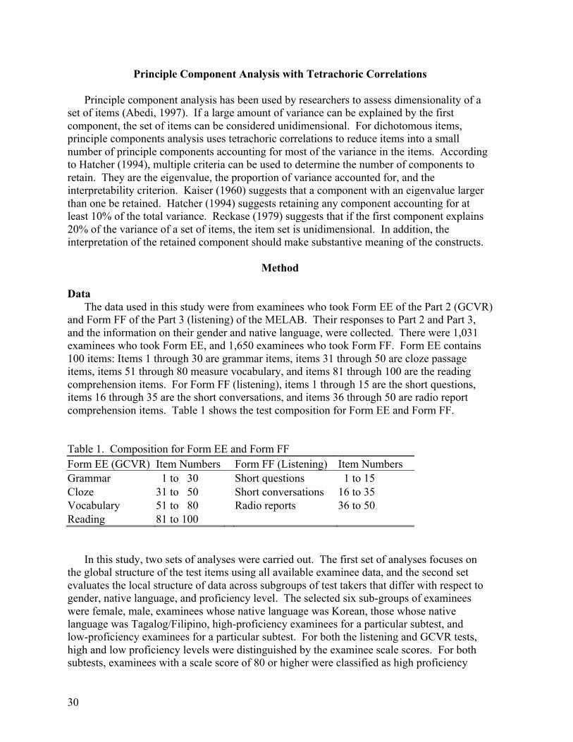
30

Principle Component Analysis with Tetrachoric Correlations Principle component analysis has been used by researchers to assess dimensionality of a

set of items (Abedi, 1997). If a large amount of variance can be explained by the first component, the set of items can be considered unidimensional. For dichotomous items, principle components analysis uses tetrachoric correlations to reduce items into a small number of principle components accounting for most of the variance in the items. According to Hatcher (1994), multiple criteria can be used to determine the number of components to retain. They are the eigenvalue, the proportion of variance accounted for, and the interpretability criterion. Kaiser (1960) suggests that a component with an eigenvalue larger than one be retained. Hatcher (1994) suggests retaining any component accounting for at least 10% of the total variance. Reckase (1979) suggests that if the first component explains 20% of the variance of a set of items, the item set is unidimensional. In addition, the interpretation of the retained component should make substantive meaning of the constructs.

Method Data

The data used in this study were from examinees who took Form EE of the Part 2 (GCVR) and Form FF of the Part 3 (listening) of the MELAB. Their responses to Part 2 and Part 3, and the information on their gender and native language, were collected. There were 1,031 examinees who took Form EE, and 1,650 examinees who took Form FF. Form EE contains 100 items: Items 1 through 30 are grammar items, items 31 through 50 are cloze passage items, items 51 through 80 measure vocabulary, and items 81 through 100 are the reading comprehension items. For Form FF (listening), items 1 through 15 are the short questions, items 16 through 35 are the short conversations, and items 36 through 50 are radio report comprehension items. Table 1 shows the test composition for Form EE and Form FF.

Table 1. Composition for Form EE and Form FF Form EE (GCVR) Item Numbers Form FF (Listening) Item Numbers Grammar 1 to 30 Short questions 1 to 15 Cloze 31 to 50 Short conversations 16 to 35 Vocabulary 51 to 80 Radio reports 36 to 50 Reading 81 to 100

In this study, two sets of analyses were carried out. The first set of analyses focuses on the global structure of the test items using all available examinee data, and the second set evaluates the local structure of data across subgroups of test takers that differ with respect to gender, native language, and proficiency level. The selected six sub-groups of examinees were female, male, examinees whose native language was Korean, those whose native language was Tagalog/Filipino, high-proficiency examinees for a particular subtest, and low-proficiency examinees for a particular subtest. For both the listening and GCVR tests, high and low proficiency levels were distinguished by the examinee scale scores. For both subtests, examinees with a scale score of 80 or higher were classified as high proficiency

31

examinees, and those with a scale score below 80 were categorized as low proficiency examinees. Due to the limited amount of data, only Tagalog/Filipino and Korean language groups were analyzed. Altogether, seven dichotomous response data sets were set up for each subtest; namely, data sets for all available examinees taking a particular subtest, female examinees, male examinees, Tagalog/Filipino speakers, Korean speakers, high-proficiency examinees, and low-proficiency examinees, resulting in 14 data sets. The number of examinees for the seven groups for each subtest is summarized in Table 2. Table 2. Number of Examinees for Each Data Set Listening Number of Examinees All examinees 1,650 Female 1,257 Male 393 Tagalog/Filipino 800 Korean 141 High listening proficiency 939 Low listening proficiency 711 GCVR All examinees 1,031 Female 787 Male 244 Tagalog/Filipino 527 Korean 123 High GCVR proficiency 528 Low GCVR proficiency 503 Procedure

After the collection of item response data, multiple procedures were adopted to appraise global and local dimensionality of the tests: Stout’s DIMTEST procedure, principle axis factoring of tetrachoric correlations, and principle components analysis with LISREL.

To calculate Stout’s statistic, test items were split into three subtests: AT1 (assessment subtest 1), AT2 (assessment subtest 2), and PT (partitioning subtest). The items in the AT1 were not specified in advance, but were identified through a principle axis factor analysis of the tetrachoric correlations by the FAC application. The FAC program first ran the tetrachoric factor analysis to calculate the second-factor loadings for the selection of AT1 subtest items set. Only part of the data was used for running FAC, while the rest of the data was used for ASN and SSC runs. The ASN program selected AT1 and AT2 items automatically based on the FAC output, and the SSC program calculated the DIMTEST statistic. SSC assessed the statistical significance of the distinctiveness of the dimensionality between two specified subtests: the Assessment Subtests and the Partitioning Subtest. DIMTSET conservative and more powerful T statistics, and their probabilities, were used as the criteria to evaluate test dimensionality, and α = 0.05 was used to determine the significance of the hypothesis test.

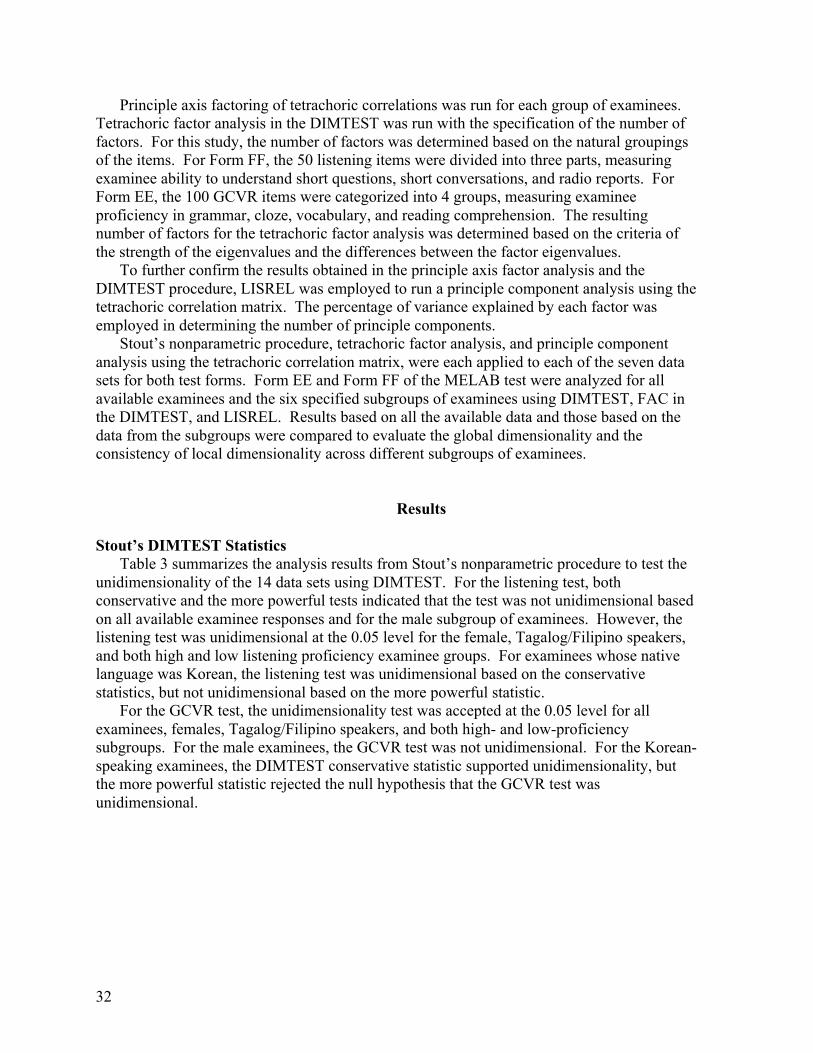
32

Principle axis factoring of tetrachoric correlations was run for each group of examinees. Tetrachoric factor analysis in the DIMTEST was run with the specification of the number of factors. For this study, the number of factors was determined based on the natural groupings of the items. For Form FF, the 50 listening items were divided into three parts, measuring examinee ability to understand short questions, short conversations, and radio reports. For Form EE, the 100 GCVR items were categorized into 4 groups, measuring examinee proficiency in grammar, cloze, vocabulary, and reading comprehension. The resulting number of factors for the tetrachoric factor analysis was determined based on the criteria of the strength of the eigenvalues and the differences between the factor eigenvalues.

To further confirm the results obtained in the principle axis factor analysis and the DIMTEST procedure, LISREL was employed to run a principle component analysis using the tetrachoric correlation matrix. The percentage of variance explained by each factor was employed in determining the number of principle components.

Stout’s nonparametric procedure, tetrachoric factor analysis, and principle component analysis using the tetrachoric correlation matrix, were each applied to each of the seven data sets for both test forms. Form EE and Form FF of the MELAB test were analyzed for all available examinees and the six specified subgroups of examinees using DIMTEST, FAC in the DIMTEST, and LISREL. Results based on all the available data and those based on the data from the subgroups were compared to evaluate the global dimensionality and the consistency of local dimensionality across different subgroups of examinees.

Results Stout’s DIMTEST Statistics

Table 3 summarizes the analysis results from Stout’s nonparametric procedure to test the unidimensionality of the 14 data sets using DIMTEST. For the listening test, both conservative and the more powerful tests indicated that the test was not unidimensional based on all available examinee responses and for the male subgroup of examinees. However, the listening test was unidimensional at the 0.05 level for the female, Tagalog/Filipino speakers, and both high and low listening proficiency examinee groups. For examinees whose native language was Korean, the listening test was unidimensional based on the conservative statistics, but not unidimensional based on the more powerful statistic.

For the GCVR test, the unidimensionality test was accepted at the 0.05 level for all examinees, females, Tagalog/Filipino speakers, and both high- and low-proficiency subgroups. For the male examinees, the GCVR test was not unidimensional. For the Korean-speaking examinees, the DIMTEST conservative statistic supported unidimensionality, but the more powerful statistic rejected the null hypothesis that the GCVR test was unidimensional.

33

Table 3. DIMTEST Results DIMTEST Statistics Conservative (T) More Powerful (T') Listening T P-value T P-value All examinees 1.991 0.023 2.254 0.012 Female 0.805 0.210 1.034 0.151 Male 2.625 0.004 3.108 0.001 Tagalog/Filipino 0.529 0.298 0.697 0.243 Korean 1.457 0.073 1.943 0.026 High listening proficiency 0.282 0.389 0.404 0.343 Low listening proficiency 0.325 0.373 0.425 0.335 GCVR All examinees -0.500 0.692 -0.473 0.682 Female 1.088 0.138 1.421 0.078 Male 1.802 0.036 2.148 0.016 Tagalog/Filipino -3.441 0.9997 -4.159 0.99998 Korean 1.288 0.099 2.176 0.015 High GCVR proficiency -0.413 0.66 -0.485 0.686 Low GCVR proficiency 0.071 0.472 -0.004 0.502 Eigenvalues and Eigenvalue Differences

The eigenvalues and the eigenvalue differences between factors for the listening test are summarized in Table 4. The eigenvalues for the first three factors were all larger than 1 for all groups. For all examinees, female, male, Tagalog/Filipino, and Korean-speaking examinee groups, the eigenvalues for the first factor were larger than 10, and the difference between the first two factors was around 10. Hattie (1985) suggests using the difference between the first factor and the second factor divided by the difference between the second and the third factor to examine the relative strength of the first factor (dubbed the Factor Difference Ratio Index (FDRI) in Johnson, Yamashiro, & Yu, 2003). If this ratio is larger than 3, the first factor is relatively strong. Based on this criterion, the data for six examinee groups: all examinees, female, male, Tagalog/Filipino speakers, Korean speakers, and low listening proficiency, satisfy this criterion. The first factor was relatively strong for these six groups of examinees. For the examinee group with high listening proficiency, the eigenvalues for the three factors were of similar strength, around 5. This data set did not meet the FDRI criterion suggested by Hattie (1985).

The eigenvalues and the eigenvalue differences between factors for the GCVR data are summarized in Table 5. The eigenvalues for the first four factors were larger than 1 for all groups. The eigenvalues for the first factor was larger than 10 for all groups, but the FDRI was greater than 3 for only all examinees, female, male, Tagalog/Filipino, and low-GCVR-proficiency examinee groups. The examinee group with high GCVR proficiency and the Korean subgroup did not satisfy Hattie’s (1985) FDRI recommendation.

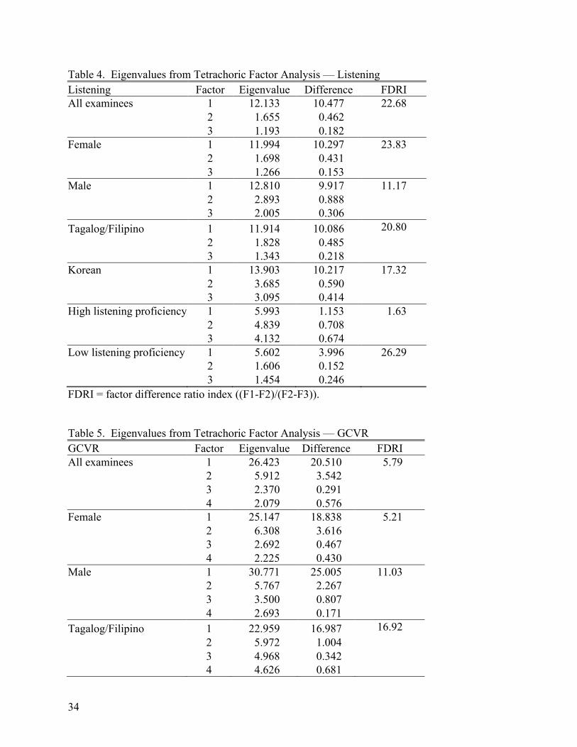
34

Table 4. Eigenvalues from Tetrachoric Factor Analysis — Listening Listening Factor Eigenvalue Difference FDRI All examinees 1 12.133 10.477 22.68 2 1.655 0.462 3 1.193 0.182 Female 1 11.994 10.297 23.83 2 1.698 0.431 3 1.266 0.153 Male 1 12.810 9.917 11.17 2 2.893 0.888 3 2.005 0.306 Tagalog/Filipino 1 11.914 10.086 20.80 2 1.828 0.485 3 1.343 0.218 Korean 1 13.903 10.217 17.32 2 3.685 0.590 3 3.095 0.414 High listening proficiency 1 5.993 1.153 1.63 2 4.839 0.708 3 4.132 0.674 Low listening proficiency 1 5.602 3.996 26.29 2 1.606 0.152 3 1.454 0.246 FDRI = factor difference ratio index ((F1-F2)/(F2-F3)). Table 5. Eigenvalues from Tetrachoric Factor Analysis — GCVR GCVR Factor Eigenvalue Difference FDRI All examinees 1 26.423 20.510 5.79 2 5.912 3.542 3 2.370 0.291 4 2.079 0.576 Female 1 25.147 18.838 5.21 2 6.308 3.616 3 2.692 0.467 4 2.225 0.430 Male 1 30.771 25.005 11.03 2 5.767 2.267 3 3.500 0.807 4 2.693 0.171 Tagalog/Filipino 1 22.959 16.987 16.92 2 5.972 1.004 3 4.968 0.342 4 4.626 0.681

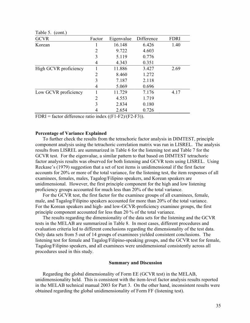
35

Table 5. (cont.) GCVR Factor Eigenvalue Difference FDRI Korean 1 16.148 6.426 1.40 2 9.722 4.603 3 5.119 0.776 4 4.343 0.351 High GCVR proficiency 1 11.886 3.427 2.69 2 8.460 1.272 3 7.187 2.118 4 5.069 0.696 Low GCVR proficiency 1 11.729 7.176 4.17 2 4.553 1.719 3 2.834 0.180 4 2.654 0.726 FDRI = factor difference ratio index ((F1-F2)/(F2-F3)). Percentage of Variance Explained

To further check the results from the tetrachoric factor analysis in DIMTEST, principle component analysis using the tetrachoric correlation matrix was run in LISREL. The analysis results from LISREL are summarized in Table 6 for the listening test and Table 7 for the GCVR test. For the eigenvalue, a similar pattern to that based on DIMTEST tetrachoric factor analysis results was observed for both listening and GCVR tests using LISREL. Using Reckase’s (1979) suggestion that a set of test items is unidimensional if the first factor accounts for 20% or more of the total variance, for the listening test, the item responses of all examinees, females, males, Tagalog/Filipino speakers, and Korean speakers are unidimensional. However, the first principle component for the high and low listening proficiency groups accounted for much less than 20% of the total variance.

For the GCVR test, the first factor for the examinee groups of all examinees, female, male, and Tagalog/Filipino speakers accounted for more than 20% of the total variance. For the Korean speakers and high- and low-GCVR-proficiency examinee groups, the first principle component accounted for less than 20 % of the total variance.

The results regarding the dimensionality of the data sets for the listening and the GCVR tests in the MELAB are summarized in Table 8. In most cases, different procedures and evaluation criteria led to different conclusions regarding the dimensionality of the test data. Only data sets from 5 out of 14 groups of examinees yielded consistent conclusions. The listening test for female and Tagalog/Filipino-speaking groups, and the GCVR test for female, Tagalog/Filipino speakers, and all examinees were unidimensional consistently across all procedures used in this study.

Summary and Discussion

Regarding the global dimensionality of Form EE (GCVR test) in the MELAB,

unidimensionality held. This is consistent with the item-level factor analysis results reported in the MELAB technical manual 2003 for Part 3. On the other hand, inconsistent results were obtained regarding the global unidimensionality of Form FF (listening test).

36

Table 6. Eigenvalues from LISREL – Listening Listening PC 1 PC 2 PC 3 All examinees Eigenvalue 12.69 2.26 1.80 % Variance 25.38 4.52 3.60 Cum. % Var 25.38 29.89 33.49 Female Eigenvalue 12.55 2.30 1.87 % Variance 25.10 4.59 3.73 Cum. % Var 25.10 29.69 33.42 Male Eigenvalue 13.24 3.03 2.24 % Variance 26.47 6.07 4.48 Cum. % Var 26.47 32.54 37.02 Tagalog/Filipino Eigenvalue 12.45 2.39 1.94 % Variance 24.90 4.79 3.88 Cum. % Var 24.90 29.69 33.57 Korean Eigenvalue 14.15 3.79 3.15 % Variance 28.30 7.58 6.31 Cum. % Var 28.30 35.89 42.19 High listening proficiency Eigenvalue 4.81 4.14 3.46 % Variance 9.62 8.28 6.39 Cum. % Var 9.62 17.91 24.83 Low listening proficiency Eigenvalue 6.18 2.33 2.18 % Variance 12.36 4.65 4.37

Cum. % Var 12.36 17.01 21.38 Table 7. Eigenvalues from LISREL — GCVR GCVR PC 1 PC 2 PC 3 PC 4 All examinees Eigenvalue 26.90 6.41 2.84 2.56 % Variance 26.90 6.41 2.84 2.56 Cum. % Var 26.90 33.32 36.15 38.72 Female Eigenvalue 25.61 6.81 3.17 2.78 % Variance 25.61 6.81 3.17 2.78 Cum. % Var 25.61 32.42 35.59 38.37 Male Eigenvalue 31.08 6.13 3.60 3.09

% Variance 31.08 6.13 3.60 3.09 Cum. % Var 31.08 37.21 40.81 43.90

Tagalog/Filipino Eigenvalue 22.03 7.57 6.39 4.35 % Variance 22.03 7.57 6.39 4.35 Cum. % Var 22.03 29.60 35.99 40.34

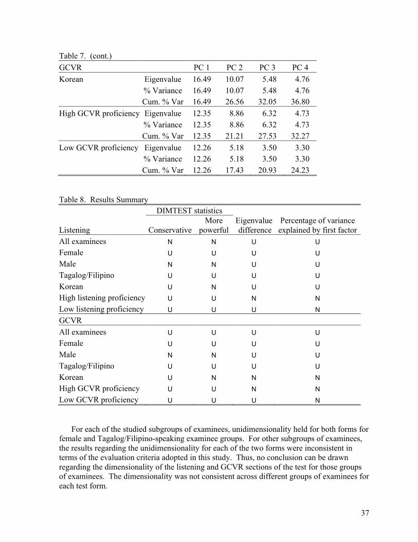
37

Table 7. (cont.) GCVR PC 1 PC 2 PC 3 PC 4 Korean Eigenvalue 16.49 10.07 5.48 4.76 % Variance 16.49 10.07 5.48 4.76 Cum. % Var 16.49 26.56 32.05 36.80 High GCVR proficiency Eigenvalue 12.35 8.86 6.32 4.73 % Variance 12.35 8.86 6.32 4.73 Cum. % Var 12.35 21.21 27.53 32.27 Low GCVR proficiency Eigenvalue 12.26 5.18 3.50 3.30

% Variance 12.26 5.18 3.50 3.30 Cum. % Var 12.26 17.43 20.93 24.23

Table 8. Results Summary

Listening

DIMTEST statistics Eigenvalue difference

Percentage of variance explained by first factor Conservative

More powerful

All examinees N N U U Female U U U U Male N N U U Tagalog/Filipino U U U U Korean U N U U High listening proficiency U U N N Low listening proficiency U U U N GCVR

All examinees U U U U Female U U U U Male N N U U Tagalog/Filipino U U U U Korean U N N N High GCVR proficiency U U N N Low GCVR proficiency U U U N

For each of the studied subgroups of examinees, unidimensionality held for both forms for

female and Tagalog/Filipino-speaking examinee groups. For other subgroups of examinees, the results regarding the unidimensionality for each of the two forms were inconsistent in terms of the evaluation criteria adopted in this study. Thus, no conclusion can be drawn regarding the dimensionality of the listening and GCVR sections of the test for those groups of examinees. The dimensionality was not consistent across different groups of examinees for each test form.

38

Several issues need attention regarding the generalizability of the study results. The first issue is related to the sample size in this study. Hatcher (1994) suggested that the minimal sample size should be 5 times the number of variables to be analyzed. Van Abswoude, et al. (2004) suggested that DIMTEST may be more effective for large sample sizes, such as n = 2,000. However, there were only data for 1,031 examinees available for the GCVR test, and 1,650 examinees for the listening test. When the subgroups of examinees were selected from these samples, much smaller samples resulted. For example, for the male and Korean groups, there were fewer than 400 cases. Sample sizes smaller than that desired may affect the analysis results.

Stout’s nonparametric procedure requires selection of the AT1 items, which was completed automatically by the program based on the second-factor loadings and other output from the FAC analysis. This study also tried to manually select AT1 items based on the tetrachoric factor analysis results. However, such selection may lead to the failure of the Wilcoxon Rank Sum Test in the ASN program. Thus, expert opinions and the factor loadings from the tetrachoric factor analysis presented in Table A.1 to Table B.7 in Appendices A and B may be combined to come up with a set of AT1 items. This may improve the DIMTEST procedure for assessing dimensionality.

In summary, the results of this study provide more information regarding the dimensionality of Part 2, listening, and Part 3, GCVR, in the MELAB. This study helps to identify the effect of the test items and of the examinees’ characteristics on the dimensionality of the MELAB sections.

Acknowledgments

I would like to express my gratitude to Dr. Shudong Wang for his insightful comments

and valuable suggestions. My thanks also go to Xueli Xu for her help on the DIMTEST program. Finally, I would like to sincerely thank Jeff Johnson for his assistance in securing the MELAB data, the information on the tests, proofreading and editing the paper.

References

Abedi, J. (1997). Dimensionality of NAEP subscale scores in mathematics (CSE Tech. Rep.

428). Los Angeles, CA: CRESST/University of California, Los Angeles. American Educational Research Association, American Psychological Association, &

National Council on Measurement in Education. (1999). Standards for educational and psychological testing. Washington, DC: American Educational Research Association.

Birenbaum, M., & Tatsuoka, K. K. (1982). On the dimensionality of achievement data. Journal of Educational Measurement, 19(4), 259-266.

Bock, R. D., Gibbons, R., & Muraki, E. (1988). Full-information item factor analysis. Applied Psychological Measurement, 12(3), 261-280.

English Language Institute, University of Michigan. (1996). MELAB technical manual. Ann Arbor, MI: English Language Institute, University of Michigan.

English Language Institute, University of Michigan. (2003). Michigan English Language Assessment Battery: Technical manual 2003. Ann Arbor, MI: English Language Institute, University of Michigan.

39

Hambleton, R. K., & Swaminathan, H. (1985). Item response theory: Principles and applications. Boston: Kluwer Nijhoff.

Hatcher, L. (1994). A step-by-step approach to using the SAS system for factor analysis and structural equation modeling. Cary, NC: SAS Institute Inc.

Hattie, J. (1985). Methodology review: Assessing unidimensionality of tests and items. Applied Psychological Measurement, 9(2), 139-164.

Johnson, J. S., Yamashiro, A., & Yu, J. (2003). ECPE annual report: 2002. Ann Arbor, MI: English Language Institute, University of Michigan.

Kaiser, H. F. (1960). The application of electronic computers to factor analysis. Educational and Psychological Measurement, 20, 141-151.

Kok, F. (1992). Differential item functioning. In L. Verhoeven, and J. H. A. L. de Jong, (Eds.), The construct of language proficiency: Applications of psychological models to language assessment (pp.115-124). Amsterdam: John Benjamins.

Messick, S. (1989). Validity. In R.L. Linn (Ed.), Educational measurement (3rd ed., pp. 13 - 103). New York: American Council on Education and Macmillan.

Messick, S. (1995). Standards-based score interpretation: Establishing valid grounds for valid inferences. In Proceedings of the joint conference on standard setting for large-scale assessments of the National Assessment Governing Board (NAGB) and the National Center for Education Statistics (NCES), Vol. II (pp. 291-305). Washington, DC: National Assessment Governing Board and National Center for Education Statistics.

Nandakumar, R. (1991). Traditional dimensionality versus essential dimensionality. Journal of Educational Measurement, 28(2), 99-118.

Nandakumar, R., & Stout, W. (1993). Refinements of Stout’s procedure for assessing latent trait unidimensionality. Journal of Educational Statistics, 18(1), 41-68.

Oltman, P. K., & Stricker, L., J. (1988, March). How native language and level of English proficiency affect the structure of the Test of English as a Foreign Language. Paper presented at the Annual Colloquium on Language Testing Research, Urbana, IL.

Reckase, M. D. (1979). Unifactor latent trait models applied to multifactor tests: Results and implications. Journal of Educational Statistics, 4(3), 207-230.

Reckase, M. D. (1985). The difficulty of test items that measure more than one ability. Applied Psychological Measurement, 9(4), 401-412.

Reckase, M. D. (1990, April). Unidimensionality data from multidimensional tests and multidimensional data from unidimensional tests. Paper presented at the Annual Meeting of the American Educational Research Association, Boston, MA.

Stout, W. F. (1987). A nonparametric approach for assessing latent trait unidimensionality. Psychometrika, 52(4), 589-617.

Stout, W. F., Goodwin Froelich, A., & Gao, F. (2001). Using resampling methods to produce an improved DIMTEST procedure. In A. Boomsma, M. A. J. van Duijin, & T. A. B. Snijders (Eds.), Essays on item response theory (pp. 357-375). New York: Springer.

van Abswoude, A. A. H., van der Ark, L. A., & Sijtsma, K. (2004). A comparative study of test data dimensionality assessment procedures under nonparametric IRT models. Applied Psychological Measurement, 28(1), 3-24.

Wang, S., & Witt, E. (2002, April). Validation and invariance of factor structure of a national licensing examination across gender and race. Paper presented at the annual meeting of the American Educational Research Association, New Orleans, LA.

40

Appendix A Factor Loadings for Form FF-Listening Table A.1. Factor Loadings for Listening- All Examinees

Item Factor Loadings

1 2 3

1 0.611 -0.078 -0.162

2 0.376 0.056 -0.199

3 0.687 -0.137 -0.122

4 0.433 0.076 0.086

5 0.435 0.024 -0.221

6 0.582 -0.161 -0.218

7 0.645 -0.088 -0.186

8 0.544 0.041 -0.101

9 0.547 0.097 -0.284

10 0.330 -0.051 -0.056

11 0.244 -0.015 -0.149

12 0.566 -0.153 0.063

13 0.386 0.104 -0.146

14 0.407 0.133 -0.080

15 0.555 0.124 -0.111

16 0.579 -0.348 0.041

17 0.686 -0.054 -0.044

18 0.484 -0.096 0.093

19 0.572 -0.153 0.187

20 0.655 -0.002 0.014

21 0.413 -0.052 -0.108

22 0.665 -0.239 0.090

23 0.737 -0.147 -0.058

24 0.530 -0.084 0.141

25 0.326 -0.153 0.219

26 0.576 -0.110 -0.024

27 0.424 0.066 -0.243

28 0.701 -0.192 0.179

29 0.696 -0.226 -0.015

30 0.368 -0.005 -0.226

31 0.481 0.070 -0.022

32 0.513 -0.216 0.134

33 0.485 0.184 -0.091

34 0.512 0.305 -0.113

35 0.312 0.048 0.063

36 0.515 -0.037 0.273

37 0.383 0.279 0.081

38 0.314 0.159 0.011

39 0.098 0.110 0.140

40 0.535 0.054 -0.095

41 0.360 0.240 0.176

42 0.339 0.280 0.145

43 0.449 0.007 0.372

44 0.515 0.163 0.215

45 0.495 0.158 0.322

46 0.259 0.502 0.012

47 0.418 0.243 0.128

48 0.270 0.166 0.118

49 0.260 0.518 -0.072

50 0.332 0.198 0.068

Table A.2. Factor Loadings for Listening-Female

Item Factor Loadings

1 2 3

1 0.620 -0.079 -0.158

2 0.393 0.006 -0.202

3 0.658 -0.176 -0.076

4 0.441 0.056 0.059

5 0.431 -0.009 -0.139

6 0.574 -0.200 -0.221

7 0.668 -0.053 -0.165

8 0.528 0.011 -0.133

9 0.517 0.049 -0.308

10 0.350 0.020 -0.036

11 0.210 -0.121 -0.168

12 0.564 -0.126 -0.011

13 0.390 0.155 -0.175

14 0.399 0.075 -0.100

15 0.547 0.074 -0.143

16 0.580 -0.365 0.122

17 0.678 -0.124 -0.019

18 0.497 -0.087 0.104

19 0.565 -0.132 0.153

20 0.611 -0.009 0.103

21 0.427 -0.004 -0.197

22 0.642 -0.190 0.043

23 0.726 -0.128 -0.064

24 0.531 -0.007 0.128

25 0.352 -0.109 0.202

26 0.605 -0.143 0.035

27 0.388 0.067 -0.248

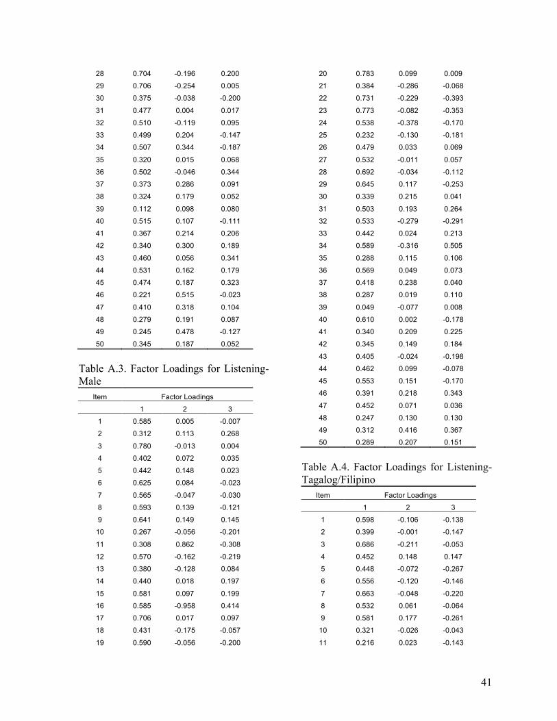
41

28 0.704 -0.196 0.200

29 0.706 -0.254 0.005

30 0.375 -0.038 -0.200

31 0.477 0.004 0.017

32 0.510 -0.119 0.095

33 0.499 0.204 -0.147

34 0.507 0.344 -0.187

35 0.320 0.015 0.068

36 0.502 -0.046 0.344

37 0.373 0.286 0.091

38 0.324 0.179 0.052

39 0.112 0.098 0.080

40 0.515 0.107 -0.111

41 0.367 0.214 0.206

42 0.340 0.300 0.189

43 0.460 0.056 0.341

44 0.531 0.162 0.179

45 0.474 0.187 0.323

46 0.221 0.515 -0.023

47 0.410 0.318 0.104

48 0.279 0.191 0.087

49 0.245 0.478 -0.127

50 0.345 0.187 0.052

Table A.3. Factor Loadings for Listening-Male

Item Factor Loadings

1 2 3

1 0.585 0.005 -0.007

2 0.312 0.113 0.268

3 0.780 -0.013 0.004

4 0.402 0.072 0.035

5 0.442 0.148 0.023

6 0.625 0.084 -0.023

7 0.565 -0.047 -0.030

8 0.593 0.139 -0.121

9 0.641 0.149 0.145

10 0.267 -0.056 -0.201

11 0.308 0.862 -0.308

12 0.570 -0.162 -0.219

13 0.380 -0.128 0.084

14 0.440 0.018 0.197

15 0.581 0.097 0.199

16 0.585 -0.958 0.414

17 0.706 0.017 0.097

18 0.431 -0.175 -0.057

19 0.590 -0.056 -0.200

20 0.783 0.099 0.009

21 0.384 -0.286 -0.068

22 0.731 -0.229 -0.393

23 0.773 -0.082 -0.353

24 0.538 -0.378 -0.170

25 0.232 -0.130 -0.181

26 0.479 0.033 0.069

27 0.532 -0.011 0.057

28 0.692 -0.034 -0.112

29 0.645 0.117 -0.253

30 0.339 0.215 0.041

31 0.503 0.193 0.264

32 0.533 -0.279 -0.291

33 0.442 0.024 0.213

34 0.589 -0.316 0.505

35 0.288 0.115 0.106

36 0.569 0.049 0.073

37 0.418 0.238 0.040

38 0.287 0.019 0.110

39 0.049 -0.077 0.008

40 0.610 0.002 -0.178

41 0.340 0.209 0.225

42 0.345 0.149 0.184

43 0.405 -0.024 -0.198

44 0.462 0.099 -0.078

45 0.553 0.151 -0.170

46 0.391 0.218 0.343

47 0.452 0.071 0.036

48 0.247 0.130 0.130

49 0.312 0.416 0.367

50 0.289 0.207 0.151

Table A.4. Factor Loadings for Listening- Tagalog/Filipino

Item Factor Loadings

1 2 3

1 0.598 -0.106 -0.138

2 0.399 -0.001 -0.147

3 0.686 -0.211 -0.053

4 0.452 0.148 0.147

5 0.448 -0.072 -0.267

6 0.556 -0.120 -0.146

7 0.663 -0.048 -0.220

8 0.532 0.061 -0.064

9 0.581 0.177 -0.261

10 0.321 -0.026 -0.043

11 0.216 0.023 -0.143

42

12 0.515 -0.121 0.122

13 0.376 0.181 -0.101

14 0.418 0.150 0.035

15 0.541 0.114 -0.139

16 0.520 -0.392 -0.020

17 0.712 -0.034 -0.019

18 0.500 -0.115 0.083

19 0.526 -0.294 0.122

20 0.592 0.030 -0.083

21 0.421 0.127 -0.111

22 0.668 -0.152 0.147

23 0.711 -0.160 -0.078

24 0.512 0.004 0.052

25 0.334 -0.291 0.266

26 0.581 -0.133 -0.120

27 0.440 0.188 -0.273

28 0.659 -0.301 0.078

29 0.693 -0.336 -0.049

30 0.345 -0.011 -0.268

31 0.505 0.093 0.087

32 0.539 -0.135 0.104

33 0.459 0.153 -0.163

34 0.514 0.385 -0.170

35 0.316 0.080 0.139

36 0.510 0.004 0.215

37 0.424 0.266 0.092

38 0.353 0.078 -0.036

39 0.097 0.146 0.237

40 0.490 0.085 -0.047

41 0.351 0.178 0.076

42 0.375 0.112 0.158

43 0.444 0.120 0.389

44 0.530 0.114 0.203

45 0.456 0.004 0.337

46 0.211 0.431 0.125

47 0.455 0.312 0.096

48 0.263 0.006 0.286

49 0.249 0.491 -0.025

50 0.376 0.207 0.182

Table A.5. Factor Loadings for Listening- Korean

Item Factor Loadings

1 2 3

1 0.639 -0.044 -0.287

2 0.370 0.242 0.105

3 0.763 0.101 0.041

4 0.473 -0.147 -0.198

5 0.501 0.130 0.163

6 0.574 0.027 -0.159

7 0.715 -0.025 -0.015

8 0.535 -0.013 -0.074

9 0.603 0.228 0.030

10 0.374 0.176 0.017

11 0.455 0.430 0.435

12 0.712 -0.162 -0.080

13 0.664 0.105 -0.206

14 0.351 0.176 0.096

15 0.607 0.096 0.139

16 0.866 -0.167 -0.786

17 0.722 -0.171 -0.110

18 0.747 -0.387 0.334

19 0.675 -0.415 0.381

20 0.719 -0.001 -0.042

21 0.459 -0.116 -0.212

22 0.480 -0.228 0.012

23 0.708 -0.062 0.031

24 0.441 0.055 -0.216

25 0.384 -0.176 0.501

26 0.566 -0.110 -0.064

27 0.001 0.660 0.534

28 0.793 -0.493 0.420

29 0.666 -0.027 0.140

30 0.322 0.128 0.191

31 0.214 0.025 -0.170

32 0.535 0.154 -0.037

33 0.468 0.362 0.157

34 0.461 0.238 -0.063

35 0.431 0.010 0.192

36 0.554 -0.086 -0.097

37 0.412 -0.048 0.010

38 0.481 0.121 -0.470

39 0.145 -0.097 -0.128

40 0.353 0.298 -0.324

41 0.333 0.429 0.339

42 0.288 0.345 0.034

43 0.530 -0.183 -0.145

44 0.507 0.091 0.126

45 0.545 0.188 -0.015

46 0.316 0.332 0.129

47 0.548 0.048 -0.006

48 -0.110 1.029 -0.467

49 0.301 0.363 0.215

50 0.322 0.140 0.024

43

Table A.6. Factor Loadings for Listening- High Proficiency

Item Factor Loadings

1 2 3

1 0.450 0.054 0.119

2 0.137 0.510 0.170

3 0.462 0.074 0.285

4 0.345 -0.144 -0.315

5 0.314 -0.057 0.407

6 0.477 -0.169 -0.004

7 0.145 0.018 0.139

8 0.128 0.175 0.067

9 0.022 0.169 -0.051

10 0.076 0.060 0.025

11 -0.026 0.586 -0.387

12 0.524 -0.489 -0.373

13 0.199 0.080 0.096

14 0.420 0.072 0.053

15 0.506 0.231 0.010

16 -1.498 0.316 -0.420

17 -0.024 0.056 -0.270

18 0.306 0.368 0.314

19 -0.133 -1.405 -0.043

20 -0.474 0.620 0.317

21 0.152 0.152 0.008

22 -0.346 -0.026 0.138

23 0.695 0.302 -0.493

24 -0.035 0.161 -0.095

25 0.282 -0.135 0.045

26 0.317 0.206 0.331

27 0.381 0.370 0.085

28 -0.179 0.059 1.388

29 0.463 0.380 -0.238

30 0.026 0.193 0.017

31 -0.034 0.459 0.066

32 0.335 -0.134 0.078

33 0.082 0.135 -0.018

34 0.133 0.188 0.188

35 0.128 -0.097 -0.009

36 -0.110 0.422 -0.451

37 -0.086 0.102 -0.008

38 0.022 0.061 -0.098

39 0.013 0.007 -0.028

40 -0.006 0.233 0.146

41 -0.154 -0.127 0.092

42 0.067 0.026 -0.028

43 -0.099 -0.075 0.238

44 -0.023 0.006 0.106

45 0.312 0.330 -0.352

46 0.087 -0.046 -0.010

47 -0.007 0.035 0.065

48 0.341 -0.027 -0.287

49 0.329 -0.109 0.146

50 -0.009 0.024 -0.014

Table A.7. Factor Loadings for Listening-Low Proficiency

Item Factor Loadings

1 2 3

1 0.398 -0.273 -0.173

2 0.056 -0.145 0.212

3 0.575 -0.169 0.204

4 0.133 0.148 -0.068

5 0.143 -0.096 0.262

6 0.425 -0.348 0.079

7 0.444 -0.264 0.009

8 0.269 0.025 0.201

9 0.165 -0.210 0.276

10 0.139 -0.141 -0.153

11 0.142 0.067 0.378

12 0.529 -0.063 -0.179

13 0.085 -0.110 -0.186

14 0.183 0.242 0.189

15 0.266 0.013 0.260

16 0.636 -0.058 0.168

17 0.524 0.036 0.180

18 0.552 0.089 0.080

19 0.473 0.035 -0.052

20 0.449 0.060 0.036

21 0.216 -0.166 -0.314

22 0.579 -0.024 -0.080

23 0.564 -0.090 0.002

24 0.316 0.173 -0.220

25 0.293 0.122 0.017

26 0.405 0.028 0.023

27 0.168 -0.074 0.124

28 0.617 0.064 -0.173

29 0.601 -0.094 0.020

30 0.134 -0.156 0.004

31 0.231 0.079 0.228

32 0.485 -0.046 -0.175

33 0.136 0.000 -0.062

34 0.064 0.093 -0.168

35 0.182 0.113 0.085

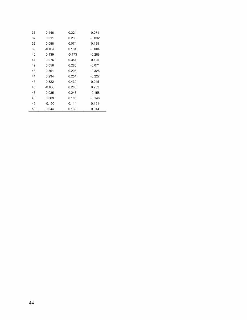
44

36 0.446 0.324 0.071

37 0.011 0.238 -0.032

38 0.088 0.074 0.139

39 -0.037 0.134 -0.004

40 0.139 -0.173 -0.288

41 0.076 0.354 0.125

42 0.056 0.288 -0.071

43 0.361 0.295 -0.325

44 0.234 0.254 -0.227

45 0.322 0.439 0.045

46 -0.066 0.268 0.202

47 0.035 0.247 -0.158

48 0.069 0.105 -0.148

49 -0.190 0.114 0.191

50 0.044 0.139 0.014

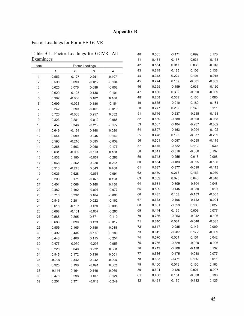
45

Appendix B Factor Loadings for Form EE-GCVR Table B.1. Factor Loadings for GCVR -All Examinees

Item Factor Loadings

1 2 3 4

1 0.553 -0.127 0.261 0.107

2 0.598 0.099 -0.012 -0.134

3 0.625 0.076 0.089 -0.002

4 0.629 -0.123 0.138 -0.101

5 0.382 -0.008 0.162 0.106

6 0.699 -0.028 0.186 -0.154

7 0.242 0.290 -0.003 -0.019

8 0.720 -0.033 0.257 0.032

9 0.323 0.281 -0.012 -0.085

10 0.457 0.346 -0.219 -0.177

11 0.649 -0.194 0.168 0.020

12 0.544 0.099 0.245 -0.140

13 0.593 -0.216 0.085 -0.032

14 0.268 0.503 0.060 -0.177

15 0.631 -0.069 -0.104 0.168

16 0.532 0.190 -0.057 -0.262

17 0.068 0.262 0.220 0.202

18 0.316 -0.243 0.343 0.488

19 0.026 0.628 -0.058 -0.091

20 0.203 0.171 -0.075 0.128

21 0.401 0.066 0.160 0.150

22 0.482 0.192 -0.007 -0.077

23 0.718 0.332 0.164 -0.080

24 0.546 0.281 0.022 -0.162

25 0.618 -0.107 0.129 -0.098

26 0.668 -0.161 -0.007 -0.265

27 0.585 0.265 0.371 -0.110

28 0.683 0.090 0.123 -0.017

29 0.559 0.165 0.188 0.015

30 0.492 0.434 -0.189 -0.183

31 0.448 0.406 0.115 -0.254

32 0.477 -0.059 -0.206 -0.055

33 0.228 0.040 0.222 0.088

34 0.545 0.172 0.136 0.001

35 -0.009 0.342 0.242 0.005

36 0.325 0.198 -0.091 0.002

37 -0.144 0.164 0.146 0.060

38 0.476 0.298 0.107 -0.124

39 0.251 0.371 -0.013 -0.249

40 0.585 -0.171 0.092 0.176

41 0.431 0.177 0.031 -0.163

42 0.554 0.017 0.038 -0.045

43 0.319 0.135 0.106 0.133

44 0.343 0.224 0.104 -0.015

45 0.274 0.189 -0.001 -0.052

46 0.365 -0.159 0.038 -0.120

47 0.430 0.309 -0.020 -0.039

48 0.258 0.369 0.130 0.085

49 0.675 -0.010 0.180 -0.164

50 0.277 0.209 0.146 0.111

51 0.716 -0.237 -0.235 -0.138

52 0.580 -0.389 -0.308 -0.088

53 0.567 -0.104 -0.257 -0.062

54 0.607 -0.163 -0.094 -0.102

55 0.478 0.193 -0.377 -0.259

56 0.501 -0.087 -0.085 -0.115

57 0.675 -0.522 0.112 0.030

58 0.641 -0.316 -0.056 0.137

59 0.743 -0.255 0.013 0.006

60 0.554 -0.183 -0.095 -0.186

61 0.637 -0.377 -0.098 -0.113

62 0.470 0.276 0.153 -0.080

63 0.382 0.070 0.046 -0.048

64 0.631 -0.309 -0.304 0.048

65 0.599 -0.145 -0.030 0.019

66 0.435 0.103 -0.153 -0.005

67 0.683 -0.196 -0.182 -0.001

68 0.651 -0.353 0.103 0.027

69 0.444 0.165 0.009 0.077

70 0.736 -0.263 -0.042 -0.106

71 0.610 0.034 -0.046 -0.085

72 0.617 -0.085 0.143 0.009

73 0.642 -0.287 0.172 -0.009

74 0.570 0.001 0.151 0.042

75 0.756 -0.329 -0.020 -0.026

76 0.719 -0.308 -0.178 0.137

77 0.566 -0.175 -0.018 0.077

78 0.633 -0.471 0.192 0.011

79 0.400 0.018 0.130 0.163

80 0.604 -0.126 0.027 -0.007

81 0.436 0.184 -0.038 0.190

82 0.421 0.160 -0.182 0.125

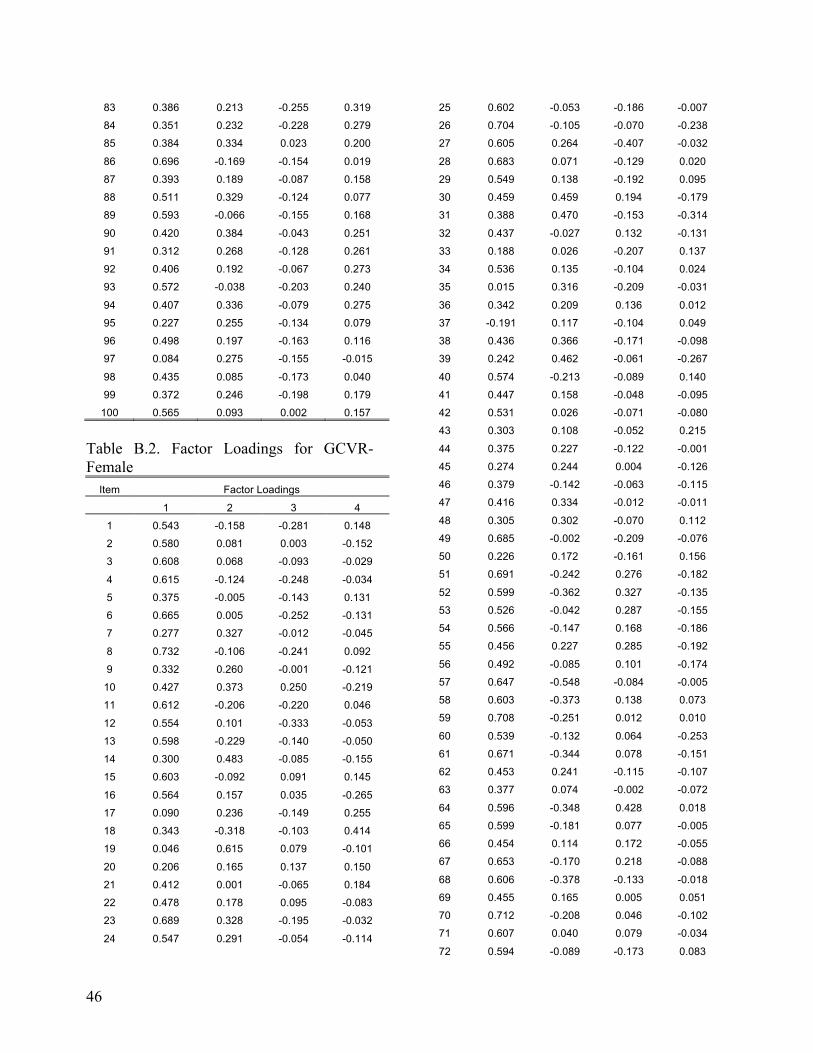
46

83 0.386 0.213 -0.255 0.319

84 0.351 0.232 -0.228 0.279

85 0.384 0.334 0.023 0.200

86 0.696 -0.169 -0.154 0.019

87 0.393 0.189 -0.087 0.158

88 0.511 0.329 -0.124 0.077

89 0.593 -0.066 -0.155 0.168

90 0.420 0.384 -0.043 0.251

91 0.312 0.268 -0.128 0.261

92 0.406 0.192 -0.067 0.273

93 0.572 -0.038 -0.203 0.240

94 0.407 0.336 -0.079 0.275

95 0.227 0.255 -0.134 0.079

96 0.498 0.197 -0.163 0.116

97 0.084 0.275 -0.155 -0.015

98 0.435 0.085 -0.173 0.040

99 0.372 0.246 -0.198 0.179

100 0.565 0.093 0.002 0.157

Table B.2. Factor Loadings for GCVR-Female

Item Factor Loadings

1 2 3 4

1 0.543 -0.158 -0.281 0.148

2 0.580 0.081 0.003 -0.152

3 0.608 0.068 -0.093 -0.029

4 0.615 -0.124 -0.248 -0.034

5 0.375 -0.005 -0.143 0.131

6 0.665 0.005 -0.252 -0.131

7 0.277 0.327 -0.012 -0.045

8 0.732 -0.106 -0.241 0.092

9 0.332 0.260 -0.001 -0.121

10 0.427 0.373 0.250 -0.219

11 0.612 -0.206 -0.220 0.046

12 0.554 0.101 -0.333 -0.053

13 0.598 -0.229 -0.140 -0.050

14 0.300 0.483 -0.085 -0.155

15 0.603 -0.092 0.091 0.145

16 0.564 0.157 0.035 -0.265

17 0.090 0.236 -0.149 0.255

18 0.343 -0.318 -0.103 0.414

19 0.046 0.615 0.079 -0.101

20 0.206 0.165 0.137 0.150

21 0.412 0.001 -0.065 0.184

22 0.478 0.178 0.095 -0.083

23 0.689 0.328 -0.195 -0.032

24 0.547 0.291 -0.054 -0.114

25 0.602 -0.053 -0.186 -0.007

26 0.704 -0.105 -0.070 -0.238

27 0.605 0.264 -0.407 -0.032

28 0.683 0.071 -0.129 0.020

29 0.549 0.138 -0.192 0.095

30 0.459 0.459 0.194 -0.179

31 0.388 0.470 -0.153 -0.314

32 0.437 -0.027 0.132 -0.131

33 0.188 0.026 -0.207 0.137

34 0.536 0.135 -0.104 0.024

35 0.015 0.316 -0.209 -0.031

36 0.342 0.209 0.136 0.012

37 -0.191 0.117 -0.104 0.049

38 0.436 0.366 -0.171 -0.098

39 0.242 0.462 -0.061 -0.267

40 0.574 -0.213 -0.089 0.140

41 0.447 0.158 -0.048 -0.095

42 0.531 0.026 -0.071 -0.080

43 0.303 0.108 -0.052 0.215

44 0.375 0.227 -0.122 -0.001

45 0.274 0.244 0.004 -0.126

46 0.379 -0.142 -0.063 -0.115

47 0.416 0.334 -0.012 -0.011

48 0.305 0.302 -0.070 0.112

49 0.685 -0.002 -0.209 -0.076

50 0.226 0.172 -0.161 0.156

51 0.691 -0.242 0.276 -0.182

52 0.599 -0.362 0.327 -0.135

53 0.526 -0.042 0.287 -0.155

54 0.566 -0.147 0.168 -0.186

55 0.456 0.227 0.285 -0.192

56 0.492 -0.085 0.101 -0.174

57 0.647 -0.548 -0.084 -0.005

58 0.603 -0.373 0.138 0.073

59 0.708 -0.251 0.012 0.010

60 0.539 -0.132 0.064 -0.253

61 0.671 -0.344 0.078 -0.151

62 0.453 0.241 -0.115 -0.107

63 0.377 0.074 -0.002 -0.072

64 0.596 -0.348 0.428 0.018

65 0.599 -0.181 0.077 -0.005

66 0.454 0.114 0.172 -0.055

67 0.653 -0.170 0.218 -0.088

68 0.606 -0.378 -0.133 -0.018

69 0.455 0.165 0.005 0.051

70 0.712 -0.208 0.046 -0.102

71 0.607 0.040 0.079 -0.034

72 0.594 -0.089 -0.173 0.083

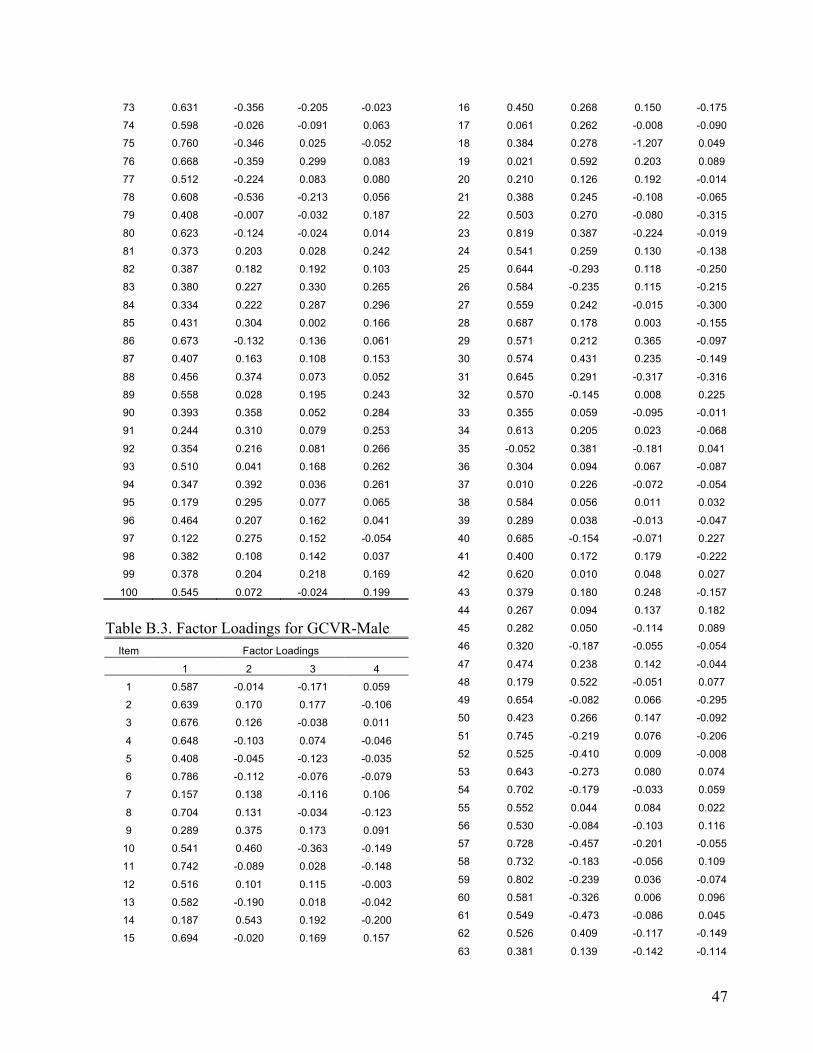
47

73 0.631 -0.356 -0.205 -0.023

74 0.598 -0.026 -0.091 0.063

75 0.760 -0.346 0.025 -0.052

76 0.668 -0.359 0.299 0.083

77 0.512 -0.224 0.083 0.080

78 0.608 -0.536 -0.213 0.056

79 0.408 -0.007 -0.032 0.187

80 0.623 -0.124 -0.024 0.014

81 0.373 0.203 0.028 0.242

82 0.387 0.182 0.192 0.103

83 0.380 0.227 0.330 0.265

84 0.334 0.222 0.287 0.296

85 0.431 0.304 0.002 0.166

86 0.673 -0.132 0.136 0.061

87 0.407 0.163 0.108 0.153

88 0.456 0.374 0.073 0.052

89 0.558 0.028 0.195 0.243

90 0.393 0.358 0.052 0.284

91 0.244 0.310 0.079 0.253

92 0.354 0.216 0.081 0.266

93 0.510 0.041 0.168 0.262

94 0.347 0.392 0.036 0.261

95 0.179 0.295 0.077 0.065

96 0.464 0.207 0.162 0.041

97 0.122 0.275 0.152 -0.054

98 0.382 0.108 0.142 0.037

99 0.378 0.204 0.218 0.169

100 0.545 0.072 -0.024 0.199

Table B.3. Factor Loadings for GCVR-Male

Item Factor Loadings

1 2 3 4

1 0.587 -0.014 -0.171 0.059

2 0.639 0.170 0.177 -0.106

3 0.676 0.126 -0.038 0.011

4 0.648 -0.103 0.074 -0.046

5 0.408 -0.045 -0.123 -0.035

6 0.786 -0.112 -0.076 -0.079

7 0.157 0.138 -0.116 0.106

8 0.704 0.131 -0.034 -0.123

9 0.289 0.375 0.173 0.091

10 0.541 0.460 -0.363 -0.149

11 0.742 -0.089 0.028 -0.148

12 0.516 0.101 0.115 -0.003

13 0.582 -0.190 0.018 -0.042

14 0.187 0.543 0.192 -0.200

15 0.694 -0.020 0.169 0.157

16 0.450 0.268 0.150 -0.175

17 0.061 0.262 -0.008 -0.090

18 0.384 0.278 -1.207 0.049

19 0.021 0.592 0.203 0.089

20 0.210 0.126 0.192 -0.014

21 0.388 0.245 -0.108 -0.065

22 0.503 0.270 -0.080 -0.315

23 0.819 0.387 -0.224 -0.019

24 0.541 0.259 0.130 -0.138

25 0.644 -0.293 0.118 -0.250

26 0.584 -0.235 0.115 -0.215

27 0.559 0.242 -0.015 -0.300

28 0.687 0.178 0.003 -0.155

29 0.571 0.212 0.365 -0.097

30 0.574 0.431 0.235 -0.149

31 0.645 0.291 -0.317 -0.316

32 0.570 -0.145 0.008 0.225

33 0.355 0.059 -0.095 -0.011

34 0.613 0.205 0.023 -0.068

35 -0.052 0.381 -0.181 0.041

36 0.304 0.094 0.067 -0.087

37 0.010 0.226 -0.072 -0.054

38 0.584 0.056 0.011 0.032

39 0.289 0.038 -0.013 -0.047

40 0.685 -0.154 -0.071 0.227

41 0.400 0.172 0.179 -0.222

42 0.620 0.010 0.048 0.027

43 0.379 0.180 0.248 -0.157

44 0.267 0.094 0.137 0.182

45 0.282 0.050 -0.114 0.089

46 0.320 -0.187 -0.055 -0.054

47 0.474 0.238 0.142 -0.044

48 0.179 0.522 -0.051 0.077

49 0.654 -0.082 0.066 -0.295

50 0.423 0.266 0.147 -0.092

51 0.745 -0.219 0.076 -0.206

52 0.525 -0.410 0.009 -0.008

53 0.643 -0.273 0.080 0.074

54 0.702 -0.179 -0.033 0.059

55 0.552 0.044 0.084 0.022

56 0.530 -0.084 -0.103 0.116

57 0.728 -0.457 -0.201 -0.055

58 0.732 -0.183 -0.056 0.109

59 0.802 -0.239 0.036 -0.074

60 0.581 -0.326 0.006 0.096

61 0.549 -0.473 -0.086 0.045

62 0.526 0.409 -0.117 -0.149

63 0.381 0.139 -0.142 -0.114

48

64 0.687 -0.175 0.095 -0.120

65 0.605 -0.026 -0.071 0.179

66 0.396 -0.063 0.206 0.137

67 0.735 -0.267 -0.194 0.173

68 0.763 -0.300 -0.091 0.118

69 0.438 0.078 -0.035 0.292

70 0.775 -0.365 0.015 -0.102

71 0.617 0.055 -0.053 -0.231

72 0.697 -0.197 0.127 -0.223

73 0.696 -0.106 0.079 -0.161

74 0.491 0.149 -0.083 -0.079

75 0.748 -0.325 -0.035 0.008

76 0.793 -0.158 0.028 0.006

77 0.676 0.034 0.062 -0.102

78 0.679 -0.322 0.017 -0.066

79 0.411 0.106 -0.456 -0.205

80 0.572 -0.248 0.049 0.031

81 0.602 0.118 0.067 -0.005

82 0.503 0.135 0.028 0.195

83 0.409 0.112 0.051 0.292

84 0.430 0.174 0.261 0.203

85 0.334 0.200 0.335 0.245

86 0.751 -0.254 0.249 0.051

87 0.374 0.190 -0.017 0.301

88 0.686 0.222 -0.259 0.270

89 0.656 -0.230 -0.232 0.034

90 0.504 0.322 0.165 0.154

91 0.471 0.181 -0.005 0.365

92 0.535 0.126 -0.081 0.329

93 0.687 -0.239 0.026 0.297

94 0.575 0.116 -0.073 0.311

95 0.349 0.191 0.069 0.160

96 0.604 0.181 -0.029 0.307

97 0.002 0.236 0.128 0.241

98 0.552 0.123 0.045 0.030

99 0.371 0.336 0.084 0.298

100 0.647 0.060 0.219 0.117

Table B.4. Factor Loadings for GCVR- Tagalog/Filipino

Item Factor Loadings

1 2 3 4

1 0.434 -0.102 0.015 -0.089

2 0.534 -0.047 -0.015 -0.048

3 0.506 -0.203 0.076 -0.051

4 0.503 -0.163 0.161 -0.094

5 0.237 0.083 0.051 -0.037

6 0.611 -0.127 0.059 -0.043

7 0.294 0.032 -0.279 -0.228

8 0.708 -0.062 0.116 -0.087

9 0.384 0.389 -0.033 -0.043

10 0.508 -0.040 -0.193 -0.458

11 0.471 -0.139 0.149 -0.012

12 0.533 -0.099 0.019 -0.054

13 0.471 -0.008 0.146 -0.234

14 0.519 0.336 -0.280 0.032

15 0.521 -0.192 0.011 -0.032

16 0.516 -0.057 -0.029 -0.053

17 0.266 0.208 0.087 0.089

18 0.357 0.066 -0.573 -1.042

19 0.348 0.377 -0.197 0.056

20 0.242 -0.010 0.186 -0.014

21 0.303 -0.004 0.091 -0.078

22 0.356 -0.147 -0.055 -0.176

23 0.927 0.025 -0.084 -0.149

24 0.685 0.183 0.016 0.018

25 0.500 -0.368 -0.345 -0.006

26 0.600 -0.152 0.148 0.052

27 0.611 -0.151 -0.014 -0.031

28 0.732 -0.206 0.111 -0.235

29 0.565 -0.194 0.041 -0.013

30 0.701 -0.055 0.106 -0.230

31 0.708 0.389 0.086 -0.079

32 0.253 -0.195 -0.337 0.371

33 0.123 0.076 -0.396 -0.232

34 0.616 -0.013 -0.045 -0.308

35 0.014 0.605 -0.204 -0.049

36 0.343 0.105 -0.070 0.228

37 -0.200 -0.001 -0.066 -0.003

38 0.594 0.216 -0.092 0.122

39 0.370 0.364 -0.132 0.169

40 0.284 0.006 0.126 0.024

41 0.504 -0.074 0.145 -0.118

42 0.468 0.074 0.032 0.250

43 0.357 0.019 0.043 0.051

44 0.385 0.107 -0.030 0.248

45 0.254 -0.082 0.121 -0.040

46 0.285 -0.201 0.064 -0.032

47 0.456 -0.164 0.075 -0.041

48 0.406 0.270 0.292 -0.234

49 0.600 -0.272 0.105 -0.079

50 0.295 0.061 0.012 0.386

51 0.524 -0.171 -0.175 0.500

52 0.298 -0.309 -0.348 0.115

53 0.351 -0.142 0.022 0.041

49

54 0.459 0.088 -0.519 0.010

55 0.475 -0.234 0.123 -0.013

56 0.349 0.159 -0.057 -0.183

57 0.654 1.131 -0.367 0.677

58 0.574 -0.103 -0.046 0.291

59 0.550 -0.285 -0.219 0.178

60 0.388 0.013 0.080 -0.152

61 0.363 -0.223 -0.602 0.211

62 0.645 0.211 -0.082 0.028

63 0.310 0.171 0.057 0.100

64 0.133 0.658 1.330 -0.104

65 0.348 0.170 0.208 -0.121

66 0.384 -0.092 0.123 0.101

67 0.510 -0.088 0.291 0.380

68 0.120 -0.047 -0.259 0.436

69 0.494 -0.153 0.071 -0.010

70 0.637 -0.323 0.158 0.073

71 0.635 -0.246 0.107 0.018

72 0.626 -0.211 -0.001 0.156

73 0.462 0.039 0.336 0.448

74 0.531 -0.286 -0.022 -0.113

75 0.485 -0.079 0.202 0.050

76 1.022 0.866 -0.188 -0.471

77 0.410 0.000 -0.012 -0.117

78 0.435 0.092 0.328 -0.355

79 0.312 0.054 -0.101 0.017

80 0.486 -0.148 0.080 0.126

81 0.371 -0.075 -0.005 0.014

82 0.366 -0.097 0.140 0.162

83 0.389 -0.050 0.008 0.154

84 0.320 -0.099 0.047 0.057

85 0.438 -0.139 0.129 0.084

86 0.516 -0.120 0.098 0.108

87 0.449 0.098 0.028 0.108

88 0.502 -0.230 -0.093 0.076

89 0.427 -0.172 0.063 0.014

90 0.689 0.052 -0.326 -0.016

91 0.395 0.072 0.033 -0.005

92 0.365 -0.146 0.053 0.027

93 0.437 -0.202 -0.002 0.145

94 0.500 -0.116 0.077 -0.249

95 0.380 0.389 -0.021 0.059

96 0.575 0.223 0.016 0.210

97 0.204 0.454 -0.076 0.023

98 0.329 -0.212 0.175 0.143

99 0.455 -0.078 0.028 -0.161

100 0.580 -0.105 0.110 0.198

Table B.5. Factor Loadings for GCVR-Korean

Item Factor Loadings

1 2 3 4

1 0.230 0.506 0.165 -0.187

2 0.644 0.022 0.131 0.145

3 0.466 0.184 -0.028 -0.240

4 0.477 0.289 0.031 0.034

5 0.137 -0.048 0.001 0.190

6 0.454 0.316 0.300 -0.020

7 0.309 0.289 -0.035 0.158

8 0.692 0.003 0.488 0.549

9 0.531 -0.053 -0.014 0.175

10 0.588 0.023 -0.101 -0.042

11 0.434 0.617 -0.108 -0.002

12 0.338 0.570 0.118 -0.118

13 0.280 0.276 -0.214 -0.211

14 0.161 0.076 -0.327 0.390

15 0.292 -0.196 0.132 0.164

16 0.354 -0.292 0.101 -0.292

17 0.020 0.084 -0.097 -0.474

18 0.121 -0.167 0.158 0.197

19 0.213 0.017 -0.095 -0.147

20 0.085 -0.517 -0.213 0.289

21 0.278 -0.328 0.037 -0.206

22 0.483 -0.187 -0.065 -0.178

23 0.249 -0.335 -0.069 0.039

24 0.524 -0.246 0.097 -0.135

25 0.316 0.415 0.097 0.055

26 0.532 0.299 0.298 0.338

27 0.307 0.706 0.463 0.149

28 0.330 -0.017 0.290 0.127

29 0.400 -0.154 0.120 -0.070

30 0.610 -0.004 0.215 -0.021

31 0.475 0.831 -0.284 -0.004

32 0.179 0.289 -0.384 0.212

33 -0.025 0.488 -0.075 -0.222

34 0.260 -0.294 0.004 -0.053

35 -0.058 -0.122 0.279 0.303

36 0.214 0.207 -0.228 0.078

37 -0.084 -0.079 -0.030 0.116

38 0.480 0.365 -0.036 -0.074

39 0.361 0.625 0.069 0.110

40 0.303 -0.095 0.019 0.268

41 0.330 0.476 0.046 -0.178

42 0.497 0.212 -0.014 0.104

43 0.252 -0.057 -0.191 0.317

50

44 0.083 -0.349 0.126 -0.129

45 0.274 0.249 0.172 -0.045

46 0.309 0.521 -0.232 -0.083

47 0.341 0.492 -0.314 0.157

48 0.278 0.146 0.052 0.128

49 0.436 0.773 -0.004 -0.027

50 -0.186 0.228 0.611 -0.212

51 0.588 -0.026 -0.229 -0.449

52 0.625 -0.505 0.101 -0.254

53 0.693 -0.431 -0.072 -0.134

54 0.439 0.246 -0.642 -0.113

55 0.540 -0.072 -0.318 -0.174

56 0.500 -0.304 0.322 -0.355

57 0.560 0.199 0.412 -0.285

58 0.357 -0.514 0.397 -0.155

59 0.454 -0.124 0.075 -0.455

60 0.543 0.078 -0.240 -0.537

61 0.559 0.301 -0.147 0.113

62 0.197 0.163 -0.082 -0.044

63 0.315 0.270 0.036 -0.043

64 0.428 -0.584 -0.188 0.038

65 0.529 -0.092 0.235 -0.098

66 0.451 -0.472 0.050 -0.199

67 0.343 -0.135 0.131 -0.081

68 0.425 -0.159 0.074 -0.095

69 0.204 -0.319 0.444 0.113

70 0.631 -0.095 0.061 0.106

71 0.451 -0.396 -0.096 -0.244

72 -0.175 -0.028 0.187 -0.019

73 0.271 -0.150 0.244 0.302

74 0.357 -0.116 -0.160 0.336

75 0.689 -0.203 0.018 0.174

76 0.365 -0.301 -0.283 0.056

77 0.352 -0.048 -0.295 -0.092

78 0.436 -0.292 0.097 -0.211

79 0.120 -0.284 0.274 -0.134

80 0.433 -0.159 0.389 -0.221

81 0.193 -0.289 -0.050 -0.040

82 0.295 0.139 0.313 0.160

83 0.214 -0.590 -0.325 0.413

84 0.474 -0.221 -0.355 0.031

85 0.233 -0.108 0.274 0.280

86 0.554 -0.202 -0.147 0.101

87 0.338 -0.148 -0.044 0.114

88 0.519 0.109 0.099 0.219

89 0.545 -0.261 -0.113 -0.044

90 0.241 -0.434 -0.272 0.333

91 0.426 -0.043 -0.434 0.217

92 0.531 -0.172 -0.234 0.012

93 0.567 0.033 -0.275 -0.029

94 0.475 0.017 0.233 0.250

95 0.242 0.272 0.148 0.267

96 0.546 -0.089 -0.022 0.170

97 0.214 0.101 -0.029 -0.042

98 0.294 0.061 -0.235 -0.008

99 0.334 -0.303 0.059 0.241

100 0.305 0.287 0.199 0.156

Table B.6. Factor Loadings for GCVR- High Proficiency

Item Factor Loadings

1 2 3 4

1 0.355 0.024 -0.346 -0.145

2 0.303 0.184 -0.123 -0.064

3 0.404 0.128 -0.348 -0.059

4 0.390 -0.307 -0.421 -0.354

5 0.153 0.179 0.133 -0.331

6 0.565 -0.224 -0.269 0.106

7 0.179 0.271 -0.084 0.095

8 0.566 -0.145 0.106 -0.087

9 0.160 0.298 0.029 0.025

10 0.309 0.368 -0.146 0.101

11 0.323 -0.263 -0.028 -0.245

12 0.534 -0.013 -0.016 0.011

13 0.416 -0.227 0.040 -0.130

14 0.359 0.526 -0.130 -0.046

15 0.304 0.141 -0.164 -0.081

16 0.417 0.255 0.348 0.002

17 0.143 0.235 -0.114 -0.075

18 0.216 -0.265 -0.246 -1.134

19 0.118 0.725 0.066 0.049

20 0.101 0.134 0.230 -0.089

21 0.294 0.134 0.101 -0.180

22 0.277 0.270 -0.122 -0.055

23 0.693 0.275 0.303 -0.193

24 0.489 0.209 0.034 -0.013

25 0.385 -0.125 -0.007 -0.208

26 0.391 -0.482 -0.170 0.258

27 0.493 0.192 -0.079 -0.188

28 0.494 -0.022 0.115 -0.057

29 0.391 0.250 0.106 -0.211

30 0.393 0.371 -0.075 0.100

31 0.307 0.372 -0.205 0.169

32 0.182 0.115 -0.279 0.479

33 0.248 0.199 -0.036 -0.182

51

34 0.457 0.090 0.153 -0.092

35 0.107 0.456 -0.033 -0.154

36 0.176 0.213 -0.102 0.158

37 -0.025 0.257 -0.114 0.007

38 0.390 0.282 -0.115 0.069

39 0.134 0.371 -0.090 0.205

40 0.336 -0.101 0.071 -0.074

41 0.380 0.181 -0.022 0.088

42 0.369 0.053 0.051 0.037

43 0.172 0.148 0.093 -0.060

44 0.310 0.167 0.053 -0.026

45 0.167 0.246 -0.394 0.123

46 0.172 -0.201 -0.079 0.070

47 0.336 0.271 -0.308 0.220

48 0.226 0.376 -0.018 -0.044

49 0.686 -0.219 -0.280 0.210

50 0.167 0.187 -0.061 -0.081

51 0.293 -0.159 -0.215 0.750

52 0.086 -0.534 0.341 0.614

53 0.320 -0.011 -0.176 0.533

54 0.293 0.060 -0.525 -0.024

55 0.137 0.311 0.007 0.118

56 0.269 -0.073 0.154 0.012

57 0.395 -0.562 -0.454 -0.374

58 0.492 -0.469 0.297 -0.195

59 0.532 -0.316 0.150 -0.190

60 0.272 -0.171 0.023 0.180

61 0.348 -0.424 0.135 0.160

62 0.475 0.165 -0.082 -0.177

63 0.324 0.221 -0.293 0.014

64 0.095 -0.211 0.595 0.296

65 0.377 -0.127 -0.438 0.048

66 0.205 -0.006 0.083 0.064

67 0.429 -0.239 0.411 0.445

68 0.389 -0.244 0.107 -0.026

69 0.507 0.108 0.407 0.031

70 0.375 -0.432 0.215 0.193

71 0.473 -0.109 0.250 0.037

72 0.568 -0.304 0.188 -0.053

73 0.565 -0.402 0.170 -0.036

74 0.503 -0.110 0.011 -0.093

75 0.477 -0.564 -0.176 0.122

76 -0.122 0.144 1.653 -0.254

77 0.453 -0.141 -0.319 0.110

78 0.576 -0.615 0.291 -0.027

79 0.326 0.096 0.019 -0.180

80 0.453 -0.141 0.224 0.152

81 0.187 0.298 0.052 -0.209

82 0.157 0.344 -0.292 0.172

83 0.108 0.386 0.180 -0.157

84 0.068 0.400 0.094 0.033

85 0.215 0.339 0.092 0.015

86 0.355 -0.200 0.209 0.093

87 0.213 0.204 0.276 0.078

88 0.283 0.417 0.080 0.071

89 0.144 0.265 0.327 0.545

90 0.304 0.431 0.347 -0.172

91 0.064 0.427 0.098 -0.042

92 0.288 0.282 0.032 -0.048

93 0.229 0.142 0.184 0.044

94 0.130 0.495 0.055 0.074

95 0.109 0.285 -0.038 0.164

96 0.181 0.307 0.110 0.030

97 -0.036 0.299 -0.049 0.154

98 0.204 0.083 0.113 0.158

99 0.206 0.354 0.131 0.021

100 0.411 0.109 0.122 0.002

Table B.7. Factor Loadings for GCVR-Low Proficiency

Item Factor Loadings

1 2 3 4

1 0.407 -0.192 0.202 0.255

2 0.266 0.257 -0.105 0.120

3 0.234 0.053 0.055 0.036

4 0.405 -0.005 0.009 0.312

5 0.184 -0.158 0.119 -0.041

6 0.305 -0.023 -0.164 0.201

7 -0.081 0.194 0.195 0.016

8 0.324 -0.122 0.298 0.333

9 0.013 0.329 -0.060 0.198

10 0.078 0.523 -0.201 -0.040

11 0.518 -0.018 0.007 0.350

12 0.087 -0.080 0.030 0.399

13 0.456 -0.124 -0.042 -0.036

14 -0.157 0.291 -0.190 -0.059

15 0.464 0.147 0.108 0.041

16 0.129 0.262 -0.442 -0.062

17 -0.157 0.020 0.453 0.212

18 0.264 -0.217 0.342 0.005

19 -0.327 0.324 -0.017 0.099

20 -0.026 0.202 0.139 -0.142

21 0.157 -0.065 0.223 0.068

22 0.205 0.299 0.036 0.196

23 -0.104 0.349 -0.287 -0.090

52

24 0.018 0.356 -0.162 0.047

25 0.366 -0.076 -0.173 0.199

26 0.441 0.114 -0.238 0.271

27 -0.019 0.083 -0.073 0.433

28 0.234 0.232 0.024 0.376

29 0.120 0.032 -0.018 0.105

30 -0.049 0.689 -0.133 0.014

31 -0.187 0.141 -0.236 0.405

32 0.377 0.134 -0.119 -0.023

33 0.116 -0.195 0.091 0.132

34 0.105 0.155 0.121 0.160

35 -0.232 -0.147 0.089 0.024

36 0.081 0.251 0.124 0.169

37 -0.190 -0.166 0.076 -0.021

38 -0.079 0.050 -0.178 0.031

39 -0.112 0.264 -0.080 0.174

40 0.467 -0.136 0.170 -0.013

41 0.074 0.128 -0.129 -0.011

42 0.284 0.005 -0.115 0.166

43 -0.003 -0.029 0.183 0.099

44 0.022 0.171 0.190 -0.048

45 0.039 0.118 0.118 0.009

46 0.228 -0.171 -0.069 0.134

47 -0.007 0.358 0.033 0.221

48 -0.154 0.177 0.242 -0.049

49 0.279 0.042 0.003 0.381

50 -0.022 0.161 0.134 0.329

51 0.687 0.158 -0.134 -0.119

52 0.638 0.084 -0.164 -0.287

53 0.444 0.156 -0.101 -0.257

54 0.524 0.070 -0.097 -0.003

55 0.229 0.433 -0.267 -0.010

56 0.317 0.002 -0.193 -0.159

57 0.764 -0.358 -0.012 -0.065

58 0.605 -0.004 0.113 -0.077

59 0.659 -0.020 -0.028 -0.006

60 0.495 0.036 -0.101 -0.103

61 0.678 -0.080 -0.097 0.068

62 -0.039 0.207 -0.059 0.032

63 0.132 -0.020 -0.096 0.036

64 0.673 0.166 -0.094 -0.127

65 0.518 0.115 0.081 0.062

66 0.176 0.360 0.092 -0.179

67 0.578 0.107 -0.004 -0.092

68 0.719 -0.205 0.012 0.079

69 -0.030 0.025 0.139 -0.140

70 0.644 0.006 -0.170 0.094

71 0.213 0.138 -0.146 -0.209

72 0.244 -0.086 -0.013 0.058

73 0.478 -0.280 -0.040 0.039

74 0.185 -0.055 0.168 -0.003

75 0.730 -0.050 -0.043 -0.045

76 0.710 0.034 0.006 -0.154

77 0.513 0.012 0.162 -0.157

78 0.622 -0.363 0.024 -0.057

79 0.220 -0.012 0.304 -0.145

80 0.432 -0.113 0.059 0.048

81 0.087 0.151 0.120 -0.033

82 0.197 0.221 0.160 -0.043

83 0.126 0.350 0.249 -0.318

84 0.154 0.402 0.325 -0.083

85 -0.032 0.272 0.331 0.125

86 0.549 0.058 0.009 -0.149

87 0.050 0.203 0.239 0.022

88 0.070 0.315 0.093 0.138

89 0.468 0.155 0.228 -0.080

90 -0.061 0.427 0.198 -0.040

91 0.041 0.257 0.214 -0.029

92 0.101 0.073 0.303 -0.301

93 0.437 0.202 0.189 -0.021

94 0.021 0.246 0.349 0.044

95 -0.021 0.216 0.104 0.149

96 0.148 0.226 0.173 -0.119

97 -0.126 0.220 -0.049 -0.066

98 0.126 0.195 -0.112 -0.045

99 0.076 0.260 0.100 -0.100

100 0.175 0.091 0.151 0.134

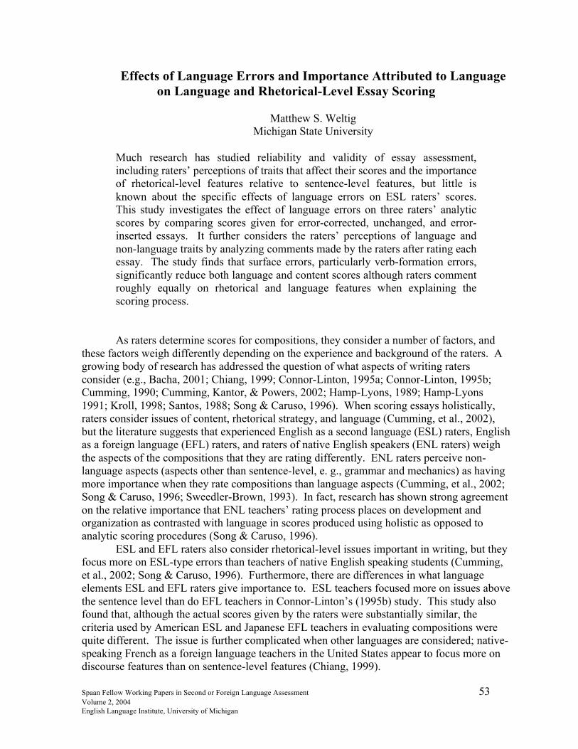
Spaan Fellow Working Papers in Second or Foreign Language Assessment 53 Volume 2, 2004 English Language Institute, University of Michigan

Effects of Language Errors and Importance Attributed to Language on Language and Rhetorical-Level Essay Scoring

Matthew S. Weltig

Michigan State University

Much research has studied reliability and validity of essay assessment, including raters’ perceptions of traits that affect their scores and the importance of rhetorical-level features relative to sentence-level features, but little is known about the specific effects of language errors on ESL raters’ scores. This study investigates the effect of language errors on three raters’ analytic scores by comparing scores given for error-corrected, unchanged, and error-inserted essays. It further considers the raters’ perceptions of language and non-language traits by analyzing comments made by the raters after rating each essay. The study finds that surface errors, particularly verb-formation errors, significantly reduce both language and content scores although raters comment roughly equally on rhetorical and language features when explaining the scoring process.

As raters determine scores for compositions, they consider a number of factors, and these factors weigh differently depending on the experience and background of the raters. A growing body of research has addressed the question of what aspects of writing raters consider (e.g., Bacha, 2001; Chiang, 1999; Connor-Linton, 1995a; Connor-Linton, 1995b; Cumming, 1990; Cumming, Kantor, & Powers, 2002; Hamp-Lyons, 1989; Hamp-Lyons 1991; Kroll, 1998; Santos, 1988; Song & Caruso, 1996). When scoring essays holistically, raters consider issues of content, rhetorical strategy, and language (Cumming, et al., 2002), but the literature suggests that experienced English as a second language (ESL) raters, English as a foreign language (EFL) raters, and raters of native English speakers (ENL raters) weigh the aspects of the compositions that they are rating differently. ENL raters perceive non-language aspects (aspects other than sentence-level, e. g., grammar and mechanics) as having more importance when they rate compositions than language aspects (Cumming, et al., 2002; Song & Caruso, 1996; Sweedler-Brown, 1993). In fact, research has shown strong agreement on the relative importance that ENL teachers’ rating process places on development and organization as contrasted with language in scores produced using holistic as opposed to analytic scoring procedures (Song & Caruso, 1996).

ESL and EFL raters also consider rhetorical-level issues important in writing, but they focus more on ESL-type errors than teachers of native English speaking students (Cumming, et al., 2002; Song & Caruso, 1996). Furthermore, there are differences in what language elements ESL and EFL raters give importance to. ESL teachers focused more on issues above the sentence level than do EFL teachers in Connor-Linton’s (1995b) study. This study also found that, although the actual scores given by the raters were substantially similar, the criteria used by American ESL and Japanese EFL teachers in evaluating compositions were quite different. The issue is further complicated when other languages are considered; native-speaking French as a foreign language teachers in the United States appear to focus more on discourse features than on sentence-level features (Chiang, 1999).

54

It is important to consider not only raters’ perceptions of the aspects of writing that affect the scores that they give but also the effect of discrete elements in the compositions. One study that addresses this issue as it relates to ENL teachers (Sweedler-Brown, 1993) found a significant difference between teachers’ perceptions of the relative importance of sentence-level grammatical errors and the holistic scores they gave. The study investigated the effects of typical ESL learners’ language errors on essays scored by having essays in which common grammatical errors were corrected and then having the corrected and uncorrected essays rated by ENL raters. Although the ENL raters agreed that “rhetorical competence,” including focus, organization, development, coherence, sense of audience, and voice, was more important than sentence-level grammatical issues, the actual holistic scores given were significantly higher for the corrected essays, and the only analytic criteria that correlated (and correlated strongly) with the holistic scores were the grammar/mechanics criteria for the uncorrected essays. In addition, for the corrected essays, grammar/mechanics and sentence structure correlated significantly, while paragraph development and organization were much less important. However, none of the raters read both the corrected and the uncorrected versions of any of the essays, so the possibility of differences among the individual raters prevents the effect of language only on the scores from being conclusively compared.

A further issue that arises is the difference in the rater’s focus when the essay is given a high rating from when it is given a low one. Cumming, et al. (2002) found that both ESL/EFL and ENL raters gave greater consideration to rhetorical skill in essays they gave a high rating to, and that the ESL/EFL raters paid more attention to language for lower scoring writers, while the ENL raters gave equal attention to language for higher and lower scoring essays. Nearly all of the essays read in Sweedler-Brown’s (1993) study were essays that were given failing scores according to the institutional guidelines when their errors were not corrected, but when the errors were corrected, nearly all were given passing grades, suggesting that those ENL raters may have graded more harshly at a lower proficiency level.

There is little research into the question of whether and how actual language and mechanics errors, as opposed to raters’ perceptions of the importance of accurate language use, interact with other traits of writing that raters consider. Sweedler-Brown’s study suggests that sentence-level errors have a very strong negative effect on raters’ judgments, whereas rhetorical features such as organization and paragraph development have very little relative effect, which is in contradiction to the criteria the raters believe they apply.

A question that arises from Sweedler-Brown’s study is whether raters are actually able to consider language elements as discrete components when rating compositions, or whether they are unable to separate language elements from the other traits they are considering. A preliminary study (Weltig, 2003) considered this question indirectly by comparing expert ESL composition teachers’ rankings of test essays that had had all of their language errors corrected to those that had not. The raters were instructed to consider only the essays’ content, not the language used, when making their rankings. The content rankings of the three raters reading corrected essays corresponded most strongly to the content rankings of the three raters reading uncorrected essays than to language or non-language scores given by the original test scorers, leading to the conclusion that expert ESL composition raters are able to consider non-language and language traits separately. However, this study did not consider the effects of the errors on the essays’ scores, but only on their relative rankings as judged by two separate groups of raters. It also did not consider error types or frequency.

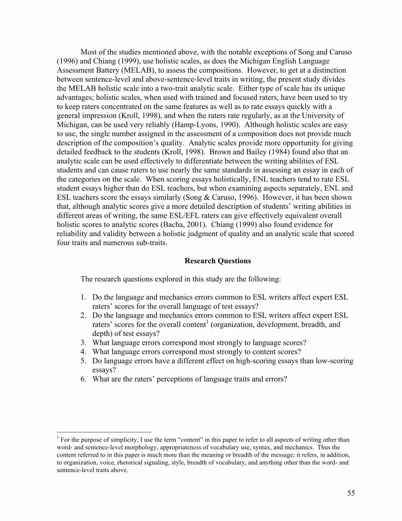
55

Most of the studies mentioned above, with the notable exceptions of Song and Caruso (1996) and Chiang (1999), use holistic scales, as does the Michigan English Language Assessment Battery (MELAB), to assess the compositions. However, to get at a distinction between sentence-level and above-sentence-level traits in writing, the present study divides the MELAB holistic scale into a two-trait analytic scale. Either type of scale has its unique advantages; holistic scales, when used with trained and focused raters, have been used to try to keep raters concentrated on the same features as well as to rate essays quickly with a general impression (Kroll, 1998), and when the raters rate regularly, as at the University of Michigan, can be used very reliably (Hamp-Lyons, 1990). Although holistic scales are easy to use, the single number assigned in the assessment of a composition does not provide much description of the composition’s quality. Analytic scales provide more opportunity for giving detailed feedback to the students (Kroll, 1998). Brown and Bailey (1984) found also that an analytic scale can be used effectively to differentiate between the writing abilities of ESL students and can cause raters to use nearly the same standards in assessing an essay in each of the categories on the scale. When scoring essays holistically, ENL teachers tend to rate ESL student essays higher than do ESL teachers, but when examining aspects separately, ENL and ESL teachers score the essays similarly (Song & Caruso, 1996). However, it has been shown that, although analytic scores give a more detailed description of students’ writing abilities in different areas of writing, the same ESL/EFL raters can give effectively equivalent overall holistic scores to analytic scores (Bacha, 2001). Chiang (1999) also found evidence for reliability and validity between a holistic judgment of quality and an analytic scale that scored four traits and numerous sub-traits.

Research Questions

The research questions explored in this study are the following: 1. Do the language and mechanics errors common to ESL writers affect expert ESL

raters’ scores for the overall language of test essays? 2. Do the language and mechanics errors common to ESL writers affect expert ESL

raters’ scores for the overall content1 (organization, development, breadth, and depth) of test essays?

3. What language errors correspond most strongly to language scores? 4. What language errors correspond most strongly to content scores? 5. Do language errors have a different effect on high-scoring essays than low-scoring

essays? 6. What are the raters’ perceptions of language traits and errors?

1 For the purpose of simplicity, I use the term “content” in this paper to refer to all aspects of writing other than word- and sentence-level morphology, appropriateness of vocabulary use, syntax, and mechanics. Thus the content referred to in this paper is much more than the meaning or breadth of the message; it refers, in addition, to organization, voice, rhetorical signaling, style, breadth of vocabulary, and anything other than the word- and sentence-level traits above.

56

Method

Essays Thirty-one essays were chosen from among 120 essays written on a single topic during

real administrations of the MELAB tests in 2001 and 2002. They had been written by hand during thirty-minute testing sessions. The examinees chose between two topics, but only essays written on a single topic were used for this project. It has been suggested that the topic of an essay may affect the student’s performance (Hamp-Lyons, 1990, 1991), which might lead to different language and non-language elements that raters have difficulty comparing. Indeed, in the preliminary study, in which the raters also taped comments as they ranked their essays, nearly half of the raters’ comments regarding how they ranked the essays had to do with the three different prompts the essays addressed (Weltig, 2003). Essays addressing a single prompt were chosen for this study so that it would be focused on the aspects of writing that influenced rating, not the student’s choice of a prompt. The writing prompt itself certainly affects the product (Hamp-Lyons, 1990; 1991), but this, as well as how students go about choosing their prompt, is a question that is addressed in other research (e.g., Polio & Glew, 1997).

The thirty-one essays were chosen for their length, variety of language proficiency and variety of content and rhetorical features. Essays with illegible handwriting were not chosen. The chosen essays were from one and one-half to two and one-half handwritten pages in length. Each essay was assigned an approximate content score and language score by the researcher for the purpose of choosing essays that would produce a variety of scores; however, because of the attempt to avoid extremely long or extremely short essays, there were no essays in which either the language score or the content score was extremely high or low.

The essays were assigned numbers for identification and typed so that the error correction and insertion would not be noticeable and in order to avoid the reduced quality of photocopies of handwriting and the effect of the quality of handwriting. The essays were typed and proofread by two experienced ESL/EFL composition teachers to ensure the original spelling, format, capitalization, and punctuation were retained. Format

Where words had been clearly stricken out by the author or erased, the words or spaces were not included in the typed version, and where arrows were clearly drawn to indicate that a word or sentence was intended for a different place, they were inserted into the intended position in the typed version. If attempts at indenting paragraphs were made, these were typed with a standard 0.5-inch indentation except for two types: if the paragraph began less than two letters to the right of the following lines, it was indicated in the typed version by a single space, and if the paragraph began approximately one-third of a page or more to the right of subsequent lines, it was typed to begin at approximately the same distance from the left margin. Where words in the original were broken at the end of a line, whether hyphenated or not, they were not broken in the typed essay.

Capitalization

Essays that were written in all capital letters were typed in all capital letters. In an essay with both capitals and lower-case letters, where a particular letter appeared to be a capital and the author used it consistently, both word-internally and word-initially, it was

57

corrected, but if it appeared at the beginnings of words, while its lower-case form appeared inside words, the word-initial capital was retained in the typed essay.

Punctuation

Where a mark appeared that looked as though it could be either a period or comma, it was typed as whichever was the more appropriate. In one essay, closing quotation marks appeared at the bottom of the line rather than the top, and the typed version attempted to imitate this position. Essay Coding

Eleven essays chosen as typical of the group were used for norming and testing inter-rater reliability. The remaining twenty essays were coded for 40 types of errors according to an adaptation of a coding system used by Sachs (2003), adapted from Polio (1997), in turn from Kroll (1990) (see Appendix A). A second reader verified the coding. Eight phrases caused initial disagreement between the readers regarding the existence of an error in the phrase. Six of these were resolved by discussion between the readers, and two were not, and so were not counted in the error totals (933 on twenty essays). Error frequencies are shown in Table 1.

Table 1. Frequency of Errors of Each Type Error code

Error

Errors per 100 words

Error code

Error

Errors per 100 words

1 aberrant clause 0.058 21 quantifier-noun agrmnt 0.000 2 subject formation 0.195 22 epenthetic pronoun 0.186 3 verb missing 0.175 23 ambiguous reference 0.215 4 verb/object complmnt 0.000 24 wrong case 0.029 5 dangling modifier 0.030 25 lexical / phrase choice 1.361 6 sentence fragment 0.369 26 idiom 0.011 7 run-on sentence 0.315 27 word form 0.317 8 parallel structure 0.068 28 noun phrase morph 0.027 9 relative clause 0.066 29 comparative formation 0.075

10 word order 0.094 30 singular for plural 1.560 11 gapping error 0.000 31 plural for singular 0.175 12 extraneous words 0.501 32 quantity words 0.070 13 missing word 0.545 33 preposition 1.920 14 wrong modal 0.101 34 genitive 0.185 15 tense / aspect 0.390 35 article 1.151 16 voice 0.178 36 deixis problem 0.063 17 verb formation 0.780 37 punctuation 2.342 18 subject-verb agree 0.353 38 negation 0.013 19 two-word verb 0.034 39 spelling 0.944 20 noun-pronoun agrmnt 0.495 40 possessive 0.082

58

Based on the initial scores assigned by the researcher, the twenty essays were roughly divided into four groups of five essays each, based on writing quality: top, upper-middle, lower-middle, and bottom. One essay was taken from each of these groups to form four new groups of five with the intention of creating four groups that were each as representative as possible of range of language and writing quality. One of these groups, the “controls” received no treatment. The other three were modified to produce three versions: unchanged essays, error-corrected essays, and error-inserted essays.

Error Correction

In error-corrected essays, all instances of errors of the seven most numerous error types (the five most numerous syntactic and semantic errors plus spelling and punctuation/mechanics) were corrected. Where consistent errors were counted as a single error, they were corrected throughout the essay. Errors of types other than those seven were unchanged (see Appendix B for examples).

Error Insertion In error-inserted essays, errors of each of the seven most numerous types were added to each essay. The average number of each type of error per hundred words in all essays was calculated (Table 1). This number was multiplied by the number of words in each essay to determine the number of errors to add, so that longer essays had more errors of each type added than shorter essays. The errors that were added were errors that appeared in the essay or were typical of other essays in the set. They were introduced into phrases in which the structure, word choice, and mechanics were target-like (see Appendix B for examples). Packet Preparation Nine packets of essays were prepared for three raters to rate three packets of essays one at a time (see Figure 1). Each packet contained 20 essays: the five control essays, five more unchanged essays, five error-corrected essays, and five error-inserted essays, as well as a scoring guide (Appendix C), and the writing prompt. The writing prompt is not reproduced here in the interest of test security.

Since raters may be influenced by the order in which they read essays, giving higher or lower scores depending on the scores of preceding essays, whether they are using a holistic or an analytic scale (Daly & Dickson-Markman, 1982; Hughes, Keeling, & Tuck, 1980), and in order to discourage the raters’ remembering how they had rated an essay with the same content previously, the essays were shuffled and renumbered so that they would be read and scored in a different order in each packet. However, to make more certain that any effects found were the effect of errors, essays with the same content were read in nearly the same order by each of the three raters for each packet. Raters

The three raters were chosen for experience rating MELAB essays, expertise in assessing ESL writing in general, and availability to work during the fall semester. Each rater was paid $150 to complete the project. Two of the raters had rated using the MELAB scale for over twelve years and the third for over a year. All of the raters also had experience rating essays using other holistic scales and analytic linguistic feature/rhetorical feature scales that were used by the University of Michigan. One of the raters had a master’s degree in TESOL

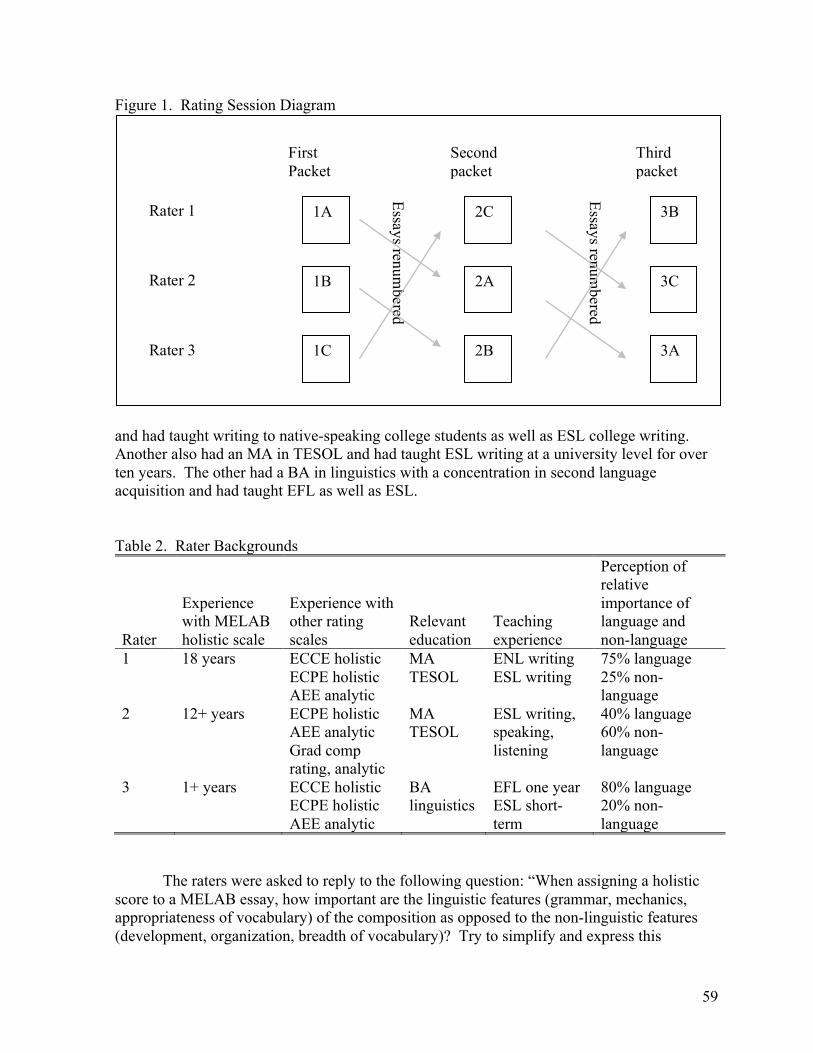
59

Figure 1. Rating Session Diagram

and had taught writing to native-speaking college students as well as ESL college writing. Another also had an MA in TESOL and had taught ESL writing at a university level for over ten years. The other had a BA in linguistics with a concentration in second language acquisition and had taught EFL as well as ESL. Table 2. Rater Backgrounds Rater

Experience with MELAB holistic scale

Experience with other rating scales

Relevant education

Teaching experience

Perception of relative importance of language and non-language

1 18 years ECCE holistic ECPE holistic AEE analytic

MA TESOL

ENL writing ESL writing

75% language 25% non-language

2 12+ years ECPE holistic AEE analytic Grad comp rating, analytic

MA TESOL

ESL writing, speaking, listening

40% language 60% non-language

3 1+ years ECCE holistic ECPE holistic AEE analytic

BA linguistics

EFL one year ESL short-term

80% language 20% non-language

The raters were asked to reply to the following question: “When assigning a holistic

score to a MELAB essay, how important are the linguistic features (grammar, mechanics, appropriateness of vocabulary) of the composition as opposed to the non-linguistic features (development, organization, breadth of vocabulary)? Try to simplify and express this

1A

1B

1C

2C 3B

2A

2B

3C

3A

Rater 2

Rater 3

First Packet

Second packet

Third packet

Rater 1

Essays renumbered

Essays renumbered

60

importance as a percentage (although deeper answers in addition are welcome).” The most experienced and the least experienced raters’ percentages were quite similar: 75% language, 25% non-language and 80% language, 20% non-language. The other rater answered 40% language and 60% non-language. One of the raters commented that non-language is much more important at the upper end of the scale. Another made a contrapositive comment that non-language is less important when control of the language starts to impede communication.

The Analytic Scale Trait descriptors for each of the ten score levels on the MELAB holistic Composition Rating Scale (English Language Institute, 1994) were divided into two categories, labeled “Content” and “Language.” Descriptors related to rhetorical features, organization, development, and cohesion were assigned to the content category, and descriptors related to syntax, morphology, and mechanics were assigned to the language category. The raters were asked to assign a score of 1-10 for content and another for language. A set of guidelines for increasing or decreasing one of these scores in cases where specific traits were particularly well or poorly expressed was also used. (Appendix C)

Although it has been noted that vocabulary can be problematic, in that some researchers consider lexical knowledge a part of pragmatic competence whereas others consider it a part of grammatical competence (Chiang, 1999), the descriptors on the MELAB rating scale divided neatly into the two categories of range and appropriate use of vocabulary. Descriptors related to range (stylistic or pragmatic features) were included in the content category, whereas descriptors related to appropriateness of vocabulary use (sentence-level features) were included in the language category. Rating

The raters met with the researcher for a ninety-minute norming session during which the raters were familiarized with the analytic scale. They were asked to consider the traits separately and not to hesitate to assign different scores for language and content. The raters read and discussed five essays so that agreement was reached on a language and content score for each essay. They were instructed to give whole-number scores, so if they felt that the language or the content of an essay lay exactly between two bands on the scale, they should round up for scores of 6-10 and down for scores of 1-5. It was noted that this system would sometimes lead to scores that would sometimes, if averaged, be different from what the raters would give on an actual MELAB test. It was also noted during this session that the fact that the essays were typed would affect their scores, since actual MELAB essays are hand-written.

Over the next two weeks, the raters rated six essays independently to check inter-rater reliability. For four of the first five essays, all three raters were within one point of each other for both content and language scores. One of the essays produced a three-point spread in content, with scores of 6, 7, and 9 given by different raters. This essay was visibly different from the others in that, as the handwritten original had been written in all capital letters, the typed version was typed in all capitals as well. A sixth essay that was typed in capitals was rated and produced the same sort of disagreement, so lower reliability was predicted for essays typed in all capital letters.

During the following five weeks, the raters rated the three packets consecutively, so that each rater rated each version of each essay (a total of 180 instances of rating, with a language and a content score for each), but (except for the control essays) each rater rated

61

each version in a different order and no rater rated the same version twice. Also, each rater recorded comments for each essay on cassette tape. The comments were taped to provide a greater quantity of more immediate comments than might be written, but a formal think-aloud protocol was not used because composition rating has been shown to be an intricate task in which numerous factors are carefully weighed (Cumming, 1990; Hamp-Lyons, 1991), and the added cognitive load of the think-aloud might have detracted from the outcome of such a complex process.

Statistical Analysis

Intra-Rater Reliability Pearson correlations of the scores assigned to the control essays for language and content were determined to check the reliability of each rater over the three rating sessions (Tables 3-8). Low numbers of scores (N = 5) resulted in several correlations that were not significant at p = 0.05, so descriptive statistics were investigated for patterns that held over the three sessions (Tables 9-14). The only clear pattern that emerged in the six sets of scores was a pattern of lower language scores assigned by rater one over time. However, the packet read last by rater one was read first by rater two, and the language scores assigned by rater two were also lower than for the other two packets, so it seems likely that the language quality of that packet was actually lower than that of the other packets. Therefore, no compensatory equations were applied to account for the separate rating sessions, and the spread among raters over the three sessions was relied upon to compensate for session differences. Table 3. Rater 1 Language Score Correlations Between Packets Language (control) Packet 2 Packet 3 Language (control) 1.000 Language packet 2 .707 1.000 Language packet 3 .866 .919* 1.000

* p < 0.05, N = 5. Table 4. Rater 2 Language Score Correlations Between Packets Language (control) Packet 2 Packet 3 Language (control) 1.000 Language packet 2 .943* 1.000 Language packet 3 .943* .786 1.000

* p < 0.05, N = 5. Table 5. Rater 3 Language Score Correlations Between Packets Language (control) Packet 2 Packet 3 Language (control) 1.000 Language packet 2 .906* 1.000 Language packet 3 .906* 1.000** 1.000

* p < 0.05, ** p < 0.01, N = 5. Table 6. Rater 1 Content Score Correlations Between Packets

62

Content (control) Packet 2 Packet 3 Content (control) 1.000 Content packet 2 .933* 1.000 Content packet 3 .933* 1.000** 1.000

* p < 0.05, ** p < 0.01, N = 5. Table 7. Rater 2 Content Score Correlations Between Packets Content (control) Packet 2 Packet 3 Content (control) 1.000 Content packet 2 .901* 1.000 Content packet 3 .824 .602 1.000

* p < 0.05, N = 5. Table 8. Rater 3 Content Score Correlations Between Packets Content (control) Packet 2 Packet 3 Content (control) 1.000 Content packet 2 .751 1.000 Content packet 3 .845 .907* 1.000

* p < 0.05, N = 5. Table 9. Rater 1 Language Score Descriptive Statistics N Minimum Maximum Mean SD Language (control) 5 3 7 5.00 1.58 Language packet 2 5 3 5 4.60 0.89 Language packet 3 5 2 5 3.80 1.10

Table 10. Rater 2 Language Score Descriptive Statistics N Minimum Maximum Mean SD Language (control) 5 2 8 4.60 2.41 Language packet 2 5 3 7 5.00 1.87 Language packet 3 5 3 8 5.00 1.87

Table 11. Rater 3 Language Score Descriptive Statistics N Minimum Maximum Mean SD Language (control) 5 3 7 5.60 1.67 Language packet 2 5 3 7 5.60 1.52 Language packet 3 5 3 7 5.60 1.52

Table 12. Rater 1 Content Score Descriptive Statistics

63

N Minimum Maximum Mean SD Content (control) 5 4 8 5.60 1.50 Content packet 2 5 4 6 5.00 0.71 Content packet 3 5 3 7 5.00 1.41

Table 13. Rater 2 Content Score Descriptive Statistics N Minimum Maximum Mean SD Content (control) 5 3 9 5.40 2.30 Content packet 2 5 3 8 5.40 2.07 Content packet 3 5 3 8 5.20 1.92

Table 14. Rater 3 Content Score Descriptive Statistics N Minimum Maximum Mean SD Content (control) 5 4 8 5.40 1.67 Content packet 2 5 3 8 5.60 1.95 Content packet 3 5 3 7 5.00 1.41

Inter-Rater Reliability Each treatment was then considered a separate instance of an essay to derive inter-rater reliability correlations at N=60 (5 control essays, 15 corrected essays, 15 unchanged essays, and 15 error-inserted essays). Pearson correlations between all pairs of raters were significant at the level of p = 0.01 for both content scores and language scores (Tables 15-16). Table 15. Inter-Rater Reliability Correlations – Language Scores Rater 1 language Rater 2 language Rater 3 language Rater 1 language 1.000 Rater 2 language .770** 1.000 Rater 3 language .746** .777** 1.000

** p < 0.01, N = 60. Table 16. Inter-Rater Reliability Correlations – Content Rater 1 content Rater 2 content Rater 3 content Rater 1 content 1.000 Rater 2 content .758** 1.000 Rater 3 content .665** .721** 1.000

** p < 0.01, N = 60. Effect of Treatment

64

To determine the effect of the treatment on the fifteen treated essays, t-tests for paired means were conducted on scores for language and content given by each rater on each treatment of the essay (corrected, uncorrected, and inserted). First, however, to ensure that scores for language and content were actually significantly different variables, a t-test for paired means was conducted on all 180 instances of rating (Table 17). The mean difference between content and language scores was 0.56, and the t-test found the difference between the content and language scores highly significant at p < 0.01. Table 17. Paired Samples Test – Content and Language

Paired Differences

Mean SD

Std. Error Mean

95% Confidence Interval of the

Difference t df Sig. (2-tailed)

Pair Lower Upper Content - Language .561 .853 .064 .436 .687 8.823 179 .000

The t-tests between original, corrected, and error-inserted essay scores indicated that correcting errors produces an average improvement in language scores of 1.067 points (out of a possible 10) and an improvement in content scores of 0.533 points, and that inserting errors produces an average reduction of 0.800 points in language scores and a reduction of 0.600 points in content scores (p < 0.01; Table 18).

Table 18. Paired Samples Test – Effect of Treatments Paired Differences

Mean SD

Std. Error Mean

95% Confidence Interval of the

Difference

t

df

Sig. (2-tailed)

Pair Lower Upper Content Corrected – No change .533 .991 .148 .236 .831 3.611 44 .001

No change – Inserted .600 .986 .147 .304 .896 4.081 44 .000

Corrected – Inserted 1.133 1.120 .167 .797 1.470 6.788 44 .000

Language Corrected – No change 1.067 .939 .140 .785 1.349 7.620 44 .000

No change – Inserted .800 1.014 .151 .495 1.105 5.295 44 .000

Corrected – Inserted 1.867 1.120 .167 1.530 2.203 11.180 44 .000

65

To test whether the presence of sentence-level errors had a greater effect on lower scores than on higher scores, the scores for treated essays were divided into three groups of fifteen by content scores. Then t-tests were conducted on the group with the highest scores and on the group with the lowest scores (Tables 19-20). Error correction had no significant effect on the high content scores, but error insertion caused an average 1.067-point drop in their content scores (p < 0.01). For the low scores, there was a significant average 0.733-point increase (p < 0.01) in content scores after error correction and an insignificant decrease in content scores after error insertion. Error correction produced a significant average language score increase in both groups (0.733 points and 1.333 points, respectively). Error insertion also caused a highly significant (p < 0.01) average decrease in language scores of 1.333 points in the top group but only a less significant (p < 0.05) 0.467-point average decrease in the language scores of the lower group. Table 19. Paired Samples Test – Top 1/3 Paired Differences

Pair Mean SD

Std. Error Mean

95% Confidence Interval of the

Difference t df Sig. (2- tailed)

Lower Upper Content Corrected – No change -.067 1.033 .267 -.639 .505 -.250 14 .806

No change – Inserted 1.067 1.163 .300 .423 1.711 3.552 14 .003

Corrected – Inserted 1.000 1.414 .365 .217 1.783 2.739 14 .016

Language Corrected – No change .733 .799 .206 .291 1.176 3.556 14 .003

No change – Inserted 1.333 .816 .211 .881 1.785 6.325 14 .000

Corrected – Inserted 2.067 1.100 .284 1.458 2.676 7.278 14 .000

66

Table 20. Paired Samples Test – Bottom 1/3 Paired Differences

Pair Mean SD

Std. Error Mean

95% Confidence Interval of the

Difference t df Sig. (2-tailed)

Lower Upper Content Corrected – No change .733 .799 .206 .291 1.176 3.556 14 .003

No change – Inserted .333 .617 .159 -.008 .675 2.092 14 .055

Corrected – Inserted 1.067 .799 .206 .624 1.509 5.172 14 .000

Language Corrected – No change 1.333 1.047 .270 .754 1.913 4.934 14 .000

No change – Inserted .467 .640 .165 .112 .821 2.824 14 .014

Corrected – Inserted 1.800 1.014 .262 1.238 2.362 6.874 14 .000

Correlations Correlations were calculated between scores (both content and language) and the other factors investigated: other (content or language) analytic score, number of words, number of errors per hundred words (error density), and error density for each type of error. (Table 21 provides the full table of correlations because, although they are outside the scope of this paper, the correlations between the errors of various types may also be of interest.) As expected, both the other analytic score and the number of words in the essay correlated strongly (p < 0.01) and positively with the content and the language scores, and the error density and density of each type of error had significant (p < 0.01) negative correlations with the scores. Therefore, a regression analysis was conducted to find out how well each factor predicted the scores.

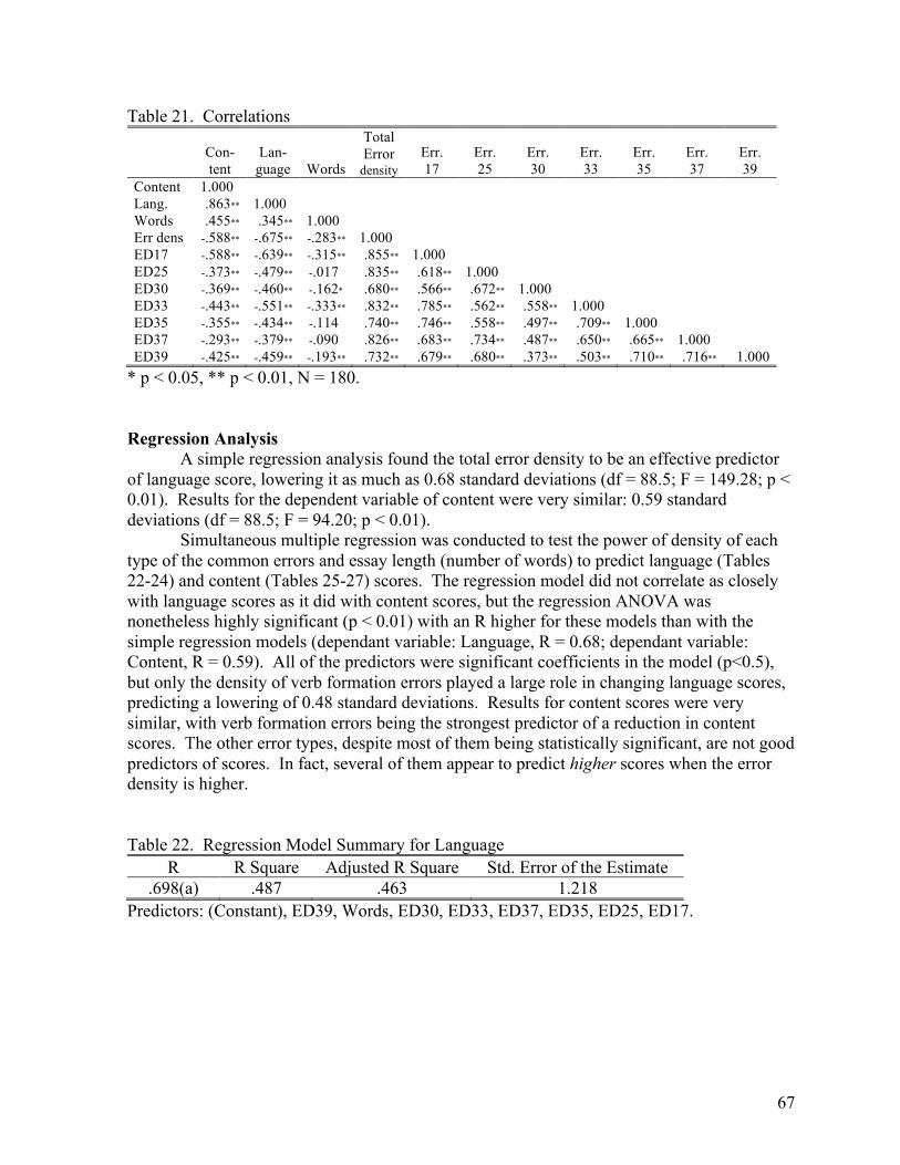
67

Table 21. Correlations

Con-tent

Lan- guage Words

Total Error

density Err. 17

Err. 25

Err. 30

Err. 33

Err. 35

Err. 37

Err. 39

Content 1.000 Lang. .863** 1.000 Words .455** .345** 1.000 Err dens -.588** -.675** -.283** 1.000 ED17 -.588** -.639** -.315** .855** 1.000 ED25 -.373** -.479** -.017 .835** .618** 1.000 ED30 -.369** -.460** -.162* .680** .566** .672** 1.000 ED33 -.443** -.551** -.333** .832** .785** .562** .558** 1.000 ED35 -.355** -.434** -.114 .740** .746** .558** .497** .709** 1.000 ED37 -.293** -.379** -.090 .826** .683** .734** .487** .650** .665** 1.000 ED39 -.425** -.459** -.193** .732** .679** .680** .373** .503** .710** .716** 1.000

* p < 0.05, ** p < 0.01, N = 180. Regression Analysis A simple regression analysis found the total error density to be an effective predictor of language score, lowering it as much as 0.68 standard deviations (df = 88.5; F = 149.28; p < 0.01). Results for the dependent variable of content were very similar: 0.59 standard deviations (df = 88.5; F = 94.20; p < 0.01). Simultaneous multiple regression was conducted to test the power of density of each type of the common errors and essay length (number of words) to predict language (Tables 22-24) and content (Tables 25-27) scores. The regression model did not correlate as closely with language scores as it did with content scores, but the regression ANOVA was nonetheless highly significant (p < 0.01) with an R higher for these models than with the simple regression models (dependant variable: Language, R = 0.68; dependant variable: Content, R = 0.59). All of the predictors were significant coefficients in the model (p<0.5), but only the density of verb formation errors played a large role in changing language scores, predicting a lowering of 0.48 standard deviations. Results for content scores were very similar, with verb formation errors being the strongest predictor of a reduction in content scores. The other error types, despite most of them being statistically significant, are not good predictors of scores. In fact, several of them appear to predict higher scores when the error density is higher. Table 22. Regression Model Summary for Language

R R Square Adjusted R Square Std. Error of the Estimate .698(a) .487 .463 1.218

Predictors: (Constant), ED39, Words, ED30, ED33, ED37, ED35, ED25, ED17.

68

Table 23. Analysis of Variance for Language Sum of Squares df Mean Square F Sig. Regression 240.658 8 30.082 20.280 .000 Residual 253.653 171 1.483 Total 494.311 179

Predictors: (Constant), ED39, Words, ED30, ED33, ED37, ED35, ED25, ED17. Table 24. Regression Analysis for Variables Predicting Language

Unstandardized

Coefficients Standardized Coefficients

B Std. Error Beta t Sig. (Constant) 5.279 .476 11.086 .000 Words .003 .001 .135 2.047 .042 ED17 -.932 .212 -.482 -4.392 .000 ED25 -.300 .149 -.221 -2.018 .045 ED30 -.081 .095 -.072 -0.859 .391 ED33 -.147 .092 -.170 -1.602 .111 ED35 .196 .157 .131 1.246 .215 ED37 .219 .077 .282 2.858 .005 ED39 -.199 .158 -.137 -1.258 .210

Table 25. Regression Summary for Content

R R Square Adjusted R

Square Std. Error of the

Estimate Durbin-Watson .892(a) .796 .784 .738 2.098

Predictors: (Constant), Language, Words, ED37, ED30, ED35, ED39, ED33, ED25, ED17, Error density. Table 26. Analysis of Variance for Content Sum of Squares df Mean Square F Sig. Regression 360.593 10 36.059 66.143 .000 Residual 92.134 169 .545 Total 452.728 179

Predictors: (Constant), Language, Words, ED37, ED30, ED35, ED39, ED33, ED25, ED17, Error density.

69

Table 27. Regression Analysis for Variables Predicting Content

Unstandardized

Coefficients Standardized Coefficients

B Std. Error Beta t Sig. (Constant) 1.478 .516 2.865 .005 Words .003 .001 .153 3.503 .001 Errordensity -.069 .027 -.413 -2.522 .013 ED17 -.231 .142 -.125 -1.621 .107 ED25 .164 .114 .126 1.440 .152 ED30 .042 .058 .039 .717 .475 ED33 .213 .064 .258 3.317 .001 ED35 .039 .096 .027 .409 .683 ED37 .108 .055 .145 1.965 .051 ED39 -.039 .096 -.028 -.405 .686 Language .694 .052 .725 13.281 .000

Comment Analysis Comments made by the raters when they rated the essays were classified according to

the “Descriptive Framework of Decision-Making Behaviors while Rating TOEFL Essays” scheme developed by Cumming, Kantor, and Powers (2002). One category of judgment strategy was added in anticipation of comments arising regarding the analytic scale: “Consider or interpret descriptors on the analytic scale.” Where a comment could be considered to be in more than one category, the more specific category was coded, unless the comment contained separate propositional content, in which case the propositions were coded separately (see Appendix E for examples). For example, the comment “It’s better than the last one” was coded as “Compare with other compositions or ‘anchors’” rather than as “Articulate general impression.” (For another example, see quote o in Appendix E. The first R11 code replaced the less specific R2.)

A total of 2,016 comments were coded for all three raters on the 180 essays: 530 by one rater, 811 by another, and 674 by the third (see Appendix D for the tallies). Because the raters were rating on an analytic scale rather than developing rating criteria to give a holistic score, and because they were recording notes rather than using a think-aloud protocol, several of the self-monitoring focus strategies outlined by Cumming, Kantor, and Powers were not found in the raters’ commentary. Also, because of the note-taking format, the raters tended to articulate each of the scores they gave (two per essay) at least once as they commented on the essay, leading to a disproportionate number of “Articulate or revise scoring decision” codes. Since the simple articulation of scores was not considered to be related to the focus of this study, the comments that simply articulated or revised scoring decisions were dropped, resulting in new totals of 1,561 total comments: 381, 675, and 505 for each rater, respectively.

The raters tended to comment slightly more on language (45.1% of the comments) than on rhetoric and ideas (40.4% of the comments). There was some variation among the raters; one rater commented on language considerably more than on rhetoric and ideas (48.8% vs. 31.8%) while the comments of the other two were more evenly balanced between focus on rhetoric and ideas (41.8% and 45.2%) and focus on language (40.4% and 48.5%).

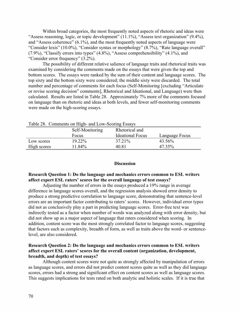
70

Within broad categories, the most frequently noted aspects of rhetoric and ideas were “Assess reasoning, logic, or topic development” (11.1%), “Assess text organization” (9.4%), and “Assess coherence” (6.1%), and the most frequently noted aspects of language were “Consider lexis” (10.0%), “Consider syntax or morphology” (8.7%), “Rate language overall” (7.9%), “Classify errors into types” (4.8%), “Assess comprehensibility” (4.1%), and “Consider error frequency” (3.2%).

The possibility of different relative salience of language traits and rhetorical traits was examined by considering the comments made on the essays that were given the top and bottom scores. The essays were ranked by the sum of their content and language scores. The top sixty and the bottom sixty were considered; the middle sixty were discarded. The total number and percentage of comments for each focus (Self-Monitoring [excluding “Articulate or revise scoring decision” comments], Rhetorical and Ideational, and Language) were then calculated. Results are listed in Table 28. Approximately 7% more of the comments focused on language than on rhetoric and ideas at both levels, and fewer self-monitoring comments were made on the high-scoring essays.

Table 28. Comments on High- and Low-Scoring Essays Self-Monitoring

Focus Rhetorical and Ideational Focus

Language Focus

Low scores 19.22% 37.21% 43.56% High scores 11.84% 40.81 47.35%

Discussion

Research Question 1: Do the language and mechanics errors common to ESL writers affect expert ESL raters’ scores for the overall language of test essays?

Adjusting the number of errors in the essays produced a 19% range in average difference in language scores overall, and the regression analysis showed error density to produce a strong predictive correlation to language score, demonstrating that sentence-level errors are an important factor contributing to raters’ scores. However, individual error types did not as conclusively play a part in predicting language scores. Error-free text was indirectly tested as a factor when number of words was analyzed along with error density, but did not show up as a major aspect of language that raters considered when scoring. In addition, content score was the most strongly correlated factor to language scores, suggesting that factors such as complexity, breadth of form, as well as traits above the word- or sentence-level, are also considered. Research Question 2: Do the language and mechanics errors common to ESL writers affect expert ESL raters’ scores for the overall content (organization, development, breadth, and depth) of test essays?

Although content scores were not quite as strongly affected by manipulation of errors as language scores, and errors did not predict content scores quite as well as they did language scores, errors had a strong and significant effect on content scores as well as language scores. This suggests implications for tests rated on both analytic and holistic scales. If it is true that

71

ESL raters “care more about” surface-level language phenomena, care should be taken to prevent them from holding back students in gate-keeping writing tests on account of surface errors. Furthermore, both for the purpose of giving appropriate feedback and in giving an honest appraisal of the skills necessary to score well on essay exams, to the degree possible without accruing deleterious psychological effects, the importance of accuracy should not be understated in a testing situation. Research Questions 3 and 4: What language errors correspond most strongly to language and content scores?

This question was not answered as conclusively, but the regression analysis suggests that errors in verb formation are more damaging to writing scores than other types of errors. Such a finding would contrast with Sweedler-Brown’s (1993) conclusion that, for ENL teachers, article errors cause the overwhelming greatest decrease in writing scores. Verb formation errors seem more likely to impede meaning and to be an important factor in communication than article errors, as well as being less persistent among very proficient second-language writers. Research Question 5: Do language errors have a different effect on high-scoring essays than low-scoring essays?

Correction of errors did not have a significant effect on the highest-scoring essays’ content scores, but error insertion did. This can be accounted for by the fact that the average number of errors per hundred words for the sample as a whole was introduced into the essays, thereby reducing the language accuracy (if defined as error-free units) of the essays. Thus naturally occurring errors would be less likely to affect content scores, as the writer would be likely to produce more accurate language. However, in cases where a writer makes persistent sentence-level errors (particularly with verb formation) despite a mastery of organization, rhetoric, and style, the essay would be expected to receive a lower content or holistic score. A similar phenomenon could be magnified for scores given for language. That is, error correction produces a strong effect on the high scoring essays, and a stronger one on the low scoring essays. Again, the slightly smaller effect at the top could be attributed to the writers’ language proficiency. However, error introduction brought about over three times the reduction in the average language scores for the high scoring essays compared to the low scoring ones.

The raters’ spoken data do not suggest that language errors have greater salience at lower proficiency levels or that rhetorical features and ideas have greater salience at higher proficiency levels. It is possible, however, considering the greater proportion of self-monitoring comments at the lower level, that raters are more confident of the scores they give for higher-level essays than lower-level essays. Research Question 6: What are the raters’ perceptions of language traits and errors?

The taped comments by the raters suggest that, when given an equal number of descriptors for content and language traits, experienced ESL raters tend to focus equally on both, with perhaps slightly more focus on language. A greater focus on language is strongly qualified, in that only two of the three raters commented more on language traits than on rhetoric and ideas and in that the analytic scale contained vocabulary descriptors in both the content and the language categories, while the categorization scheme for the comments

72

contained only one category, “Consider lexis,” which fell into the language focus area. In addition, the language section of the scale has slightly more descriptors than the content section, which also probably influenced the raters’ comments.

Rater comments most generally had corollaries on the scoring guide, suggesting that the raters were using the guide effectively to guide them in determining their scores. In particular, the three most common rhetorical and ideational focus strategies, “Assess reasoning, logic, or topic development,” “Assess text organization,” and “Assess coherence” are found repeatedly in the scoring guide, which refers to topic development, organization, and connection. Also, two of the most common language focus strategies, “Consider lexis” and “Consider syntax or morphology,” are implied by the vocabulary descriptors in both the language and content sections and the language descriptors that refer to syntactic structures and morphological control. Many of the other frequent language focus strategies also have indirect corollaries on the scoring guide: “Assess comprehensibility” is implied by descriptors referring to inhibiting communication, “Consider error frequency,” by descriptors including phrases like “nearly always” at the top of the scale and “often” at the bottom, “Rate language overall,” by descriptors referring to flexible use and simple or complex language, and “Classify errors into types,” by descriptors referring to “wide range.” It is interesting that fluency and spelling and punctuation, which are also mentioned on the scoring guide, and error gravity, which is implied by the scoring guide, are mentioned relatively infrequently.

In addition to the questions this paper was intended to address, several other questions are relevant to this study. Reasons for different context effects in different raters and how they may be controlled are issues that will aid in maintaining reliable rating of writing. Another interesting question that unexpectedly came up in this study is that of the effects of writing and typing all in capital letters on inter-rater reliability. Only one of the fifteen treated essays (and none of the controls), in addition to the two used during norming and reliability testing, was originally written in all caps, so no conclusions can be drawn from the present study. However, on that essay, the raters’ scores ranged from 2-4 in language and 4-6 in content when it was unchanged and when errors were inserted, but when the capitalization was corrected, the range was only from 4-5 in language and 5-6 in content.

Some limitations of the present study include limits to its generalizability. The reliability of the raters is sufficient to warrant conclusions about experienced MELAB raters, but since there were only three of them, it is not appropriate to generalize findings of the study to ESL composition raters in general. Also, although the manipulation of the essays in this study and the repeated rating of each version yielded large N sizes, from which valid conclusions can be drawn about errors typical of this sample, other samples might yield different types and densities of errors. In the twenty essays examined, three of the error types in the classification system did not occur. Furthermore, the prompt may have influenced the errors. For example, the nature of this prompt caused the majority of the writers to use the word “clothes” (correctly) or another lexical choice such as “dresses” incorrectly, affecting the number of lexical choice errors in this study. Further research might elucidate clearer relationships between language errors and writing prompts. Another limitation of this study might be that the effects of introducing errors into essays that scored high in non-language categories suggest the possibility of increased salience of surface errors in higher proficiency writing. A related effect concerns the unnaturalness of low-proficiency errors in high-proficiency writing. One rater noticed and commented on this (see Appendix E, quote f). Although several of the errors she mentioned as sounding unnatural were actually real learner

73

errors in an unchanged control essay, the error frequency in the error-inserted essays probably made them more salient, so that even natural errors began to sound unnatural. Because this effect was not brought up during the first two packets, its effect is probably not major. However, if future error-insertion studies are done, the effect of proficiency on error type should be considered in the experimental design. Finally, the spoken data were coded by only one person, so the reliability of the coding was not estimated. However, the brevity of comments for each essay, since these were spoken notes rather than think-aloud protocols, was such that high reliability would be anticipated.

Acknowledgments

I would like to thank Mary Spaan and the English Language Institute of the University

of Michigan for the support and materials that allowed me to undertake this project. I would especially like to thank Jeff Johnson and Mary Spaan for their suggestions and feedback on the project’s design and the three raters for their patience and toil during one of the busiest times of the academic year. In addition, I would like to thank my untiring research assistant and dear wife, Yan Wang, for all of her trips to the library, typing, essay reading, checking, and general support.

References

Bacha, N. (2001). Writing evaluation: What can analytic versus holistic essay scoring tell us?

System 29(3), 371-383. Brown, J.D., & Bailey, K.M. (1984). A categorical instrument for scoring second language

writing skills. Language Learning, 34(4), 21-42. Chiang, S.Y. (1999). Assessing grammatical and textual features in L2 writing samples: The

case of French as a foreign language. The Modern Language Journal, 83(ii), 219-232. Connor-Linton, J. (1995a). Crosscultural comparison of writing standards: American ESL and

Japanese EFL. World Englishes, 14(1), 99-115. Connor-Linton, J. (1995b). Looking behind the curtain: What do L2 composition ratings

really mean? TESOL Quarterly, 29(4), 762-765. Cumming, A. (1990). Expertise in evaluating second language compositions. Language

Testing, 7(1), 31-51. Cumming, A., Kantor, R. & Powers, D. E. (2002). Decision making while rating ESL/EFL

writing tasks: A descriptive framework. The Modern Language Journal, 86(i), 67-96. Daly, J. A., & Dickson-Markman, F. (1982). Contrast effects in evaluating essays. Journal of

Educational Measurement, 19(4), 309-316. English Language Institute, University of Michigan. (1994). MELAB technical manual. Ann

Arbor, MI: English Language Institute, University of Michigan. Hamp-Lyons, L. (1989). Raters respond to rhetoric in writing. In H. Dechert & G. Raupach

(Eds.), Interlingual processes (pp. 229-244). Turbingen, Germany: Gunter Narr Verlag.

Hamp-Lyons, L. (1990). Second language writing: Assessment issues. In B. Kroll (Ed.), Second language writing: Research insights for the classroom (pp. 69-87). Cambridge: Cambridge University Press.

74

Hamp-Lyons, L. (1991). Assessing second language writing in academic contexts. Norwood, NJ: Ablex.

Hughes, D. C., Keeling, B., & Tuck, B. F. (1980). The influence of context position and scoring method on essay scoring. Journal of Educational Measurement, 17(2), 131-135.

Kroll, B. (1990). What does time buy? ESL student performance on home versus class compositions. In B. Kroll (Ed.), Second language writing: Research insights for the classroom (pp. 140-154). Cambridge: Cambridge University Press.

Kroll, B. (1998). Assessing writing abilities. Annual Review of Applied Linguistics, 18, 219-240.

Polio, C. G. (1997). Measures of linguistic accuracy in second language writing research. Language Learning, 47(1), 101-143.

Polio, C., & Glew, M. (1996). ESL writing assessment prompts: How students choose. Journal of Second Language Writing, 5(1), 35-49.

Santos, T. (1988). Professors’ reactions to the academic writing of nonnative-speaking students. TESOL Quarterly, 22(1), 69-90.

Sachs, R. (2003). Reformulation, noticing, and second language writing. Unpublished master’s thesis, Michigan State University, East Lansing, Michigan.

Song, B., & Caruso, I. (1996). Do English and ESL faculty differ in evaluating the essays of native English-speaking and ESL students? Journal of Second Language Writing, 5(2), 163-182.

Sweedler-Brown, C.O. (1993). ESL essay evaluation: The influence of sentence-level and rhetorical features. Journal of Second Language Writing, 2(1), 3-17.

Weltig, M. (2003, March). Distinguishing content from language in essay assessment. Paper presented at the annual convention of Teachers of English to Speakers of Other Languages, Baltimore, MD.

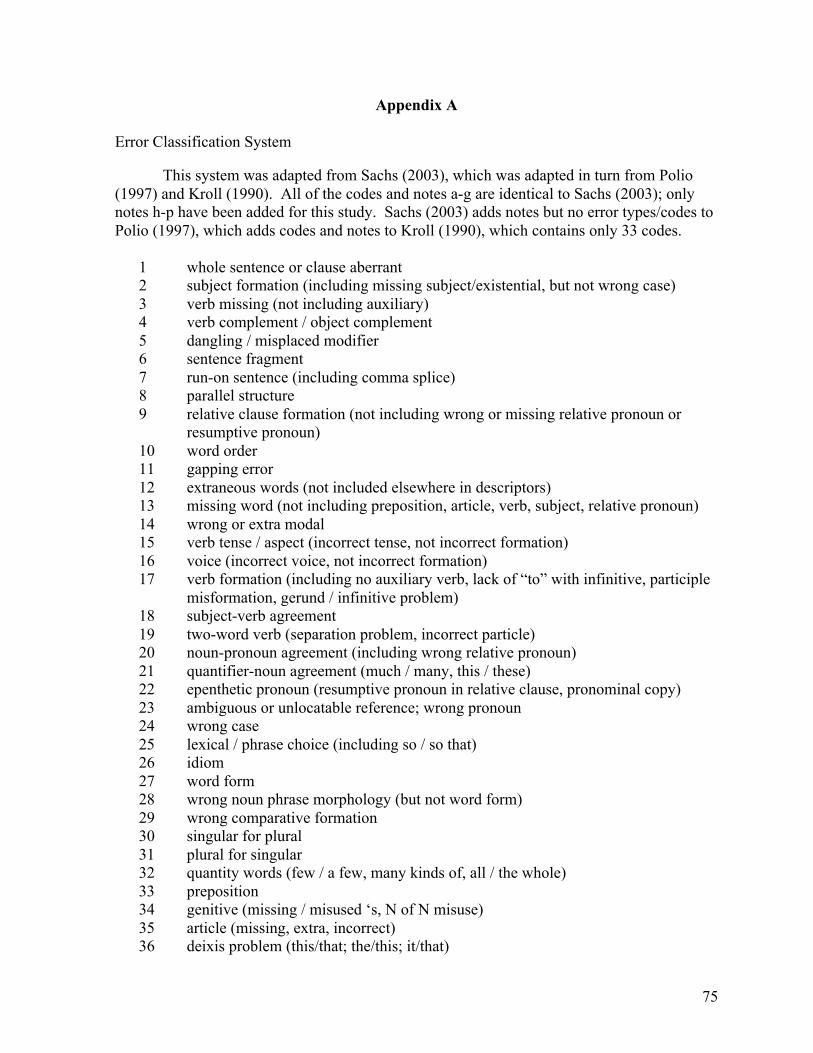
75

Appendix A Error Classification System This system was adapted from Sachs (2003), which was adapted in turn from Polio (1997) and Kroll (1990). All of the codes and notes a-g are identical to Sachs (2003); only notes h-p have been added for this study. Sachs (2003) adds notes but no error types/codes to Polio (1997), which adds codes and notes to Kroll (1990), which contains only 33 codes.

1 whole sentence or clause aberrant 2 subject formation (including missing subject/existential, but not wrong case) 3 verb missing (not including auxiliary) 4 verb complement / object complement 5 dangling / misplaced modifier 6 sentence fragment 7 run-on sentence (including comma splice) 8 parallel structure 9 relative clause formation (not including wrong or missing relative pronoun or

resumptive pronoun) 10 word order 11 gapping error 12 extraneous words (not included elsewhere in descriptors) 13 missing word (not including preposition, article, verb, subject, relative pronoun) 14 wrong or extra modal 15 verb tense / aspect (incorrect tense, not incorrect formation) 16 voice (incorrect voice, not incorrect formation) 17 verb formation (including no auxiliary verb, lack of “to” with infinitive, participle

misformation, gerund / infinitive problem) 18 subject-verb agreement 19 two-word verb (separation problem, incorrect particle) 20 noun-pronoun agreement (including wrong relative pronoun) 21 quantifier-noun agreement (much / many, this / these) 22 epenthetic pronoun (resumptive pronoun in relative clause, pronominal copy) 23 ambiguous or unlocatable reference; wrong pronoun 24 wrong case 25 lexical / phrase choice (including so / so that) 26 idiom 27 word form 28 wrong noun phrase morphology (but not word form) 29 wrong comparative formation 30 singular for plural 31 plural for singular 32 quantity words (few / a few, many kinds of, all / the whole) 33 preposition 34 genitive (missing / misused ‘s, N of N misuse) 35 article (missing, extra, incorrect) 36 deixis problem (this/that; the/this; it/that)

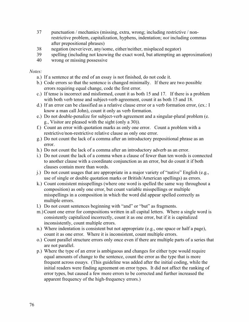
76

37 punctuation / mechanics (missing, extra, wrong; including restrictive / non-restrictive problem, capitalization, hyphens, indentation; not including commas after prepositional phrases)

38 negation (never/ever, any/some, either/neither, misplaced negator) 39 spelling (including not knowing the exact word, but attempting an approximation) 40 wrong or missing possessive

Notes:

a.) If a sentence at the end of an essay is not finished, do not code it. b.) Code errors so that the sentence is changed minimally. If there are two possible

errors requiring equal change, code the first error. c.) If tense is incorrect and misformed, count it as both 15 and 17. If there is a problem

with both verb tense and subject-verb agreement, count it as both 15 and 18. d.) If an error can be classified as a relative clause error or a verb formation error, (ex.: I

know a man call John), count it only as verb formation. e.) Do not double-penalize for subject-verb agreement and a singular-plural problem (e.

g., Visitor are pleased with the sight (only a 30)). f.) Count an error with quotation marks as only one error. Count a problem with a

restrictive/non-restrictive relative clause as only one error. g.) Do not count the lack of a comma after an introductory prepositional phrase as an

error. h.) Do not count the lack of a comma after an introductory adverb as an error. i.) Do not count the lack of a comma when a clause of fewer than ten words is connected

to another clause with a coordinate conjunction as an error, but do count it if both clauses contain more than words.

j.) Do not count usages that are appropriate in a major variety of “native” English (e.g., use of single or double quotation marks or British/American spellings) as errors.

k.) Count consistent misspellings (where one word is spelled the same way throughout a composition) as only one error, but count variable misspellings or multiple misspellings in a composition in which the word did appear spelled correctly as multiple errors.

l.) Do not count sentences beginning with “and” or “but” as fragments. m.) Count one error for compositions written in all capital letters. Where a single word is

consistently capitalized incorrectly, count it as one error, but if it is capitalized inconsistently, count multiple errors.

n.) Where indentation is consistent but not appropriate (e.g., one space or half a page), count it as one error. Where it is inconsistent, count multiple errors.

o.) Count parallel structure errors only once even if there are multiple parts of a series that are not parallel.

p.) Where the type of an error is ambiguous and changes for either type would require equal amounts of change to the sentence, count the error as the type that is more frequent across essays. (This guideline was added after the initial coding, while the initial readers were finding agreement on error types. It did not affect the ranking of error types, but caused a few more errors to be corrected and further increased the apparent frequency of the high-frequency errors.)

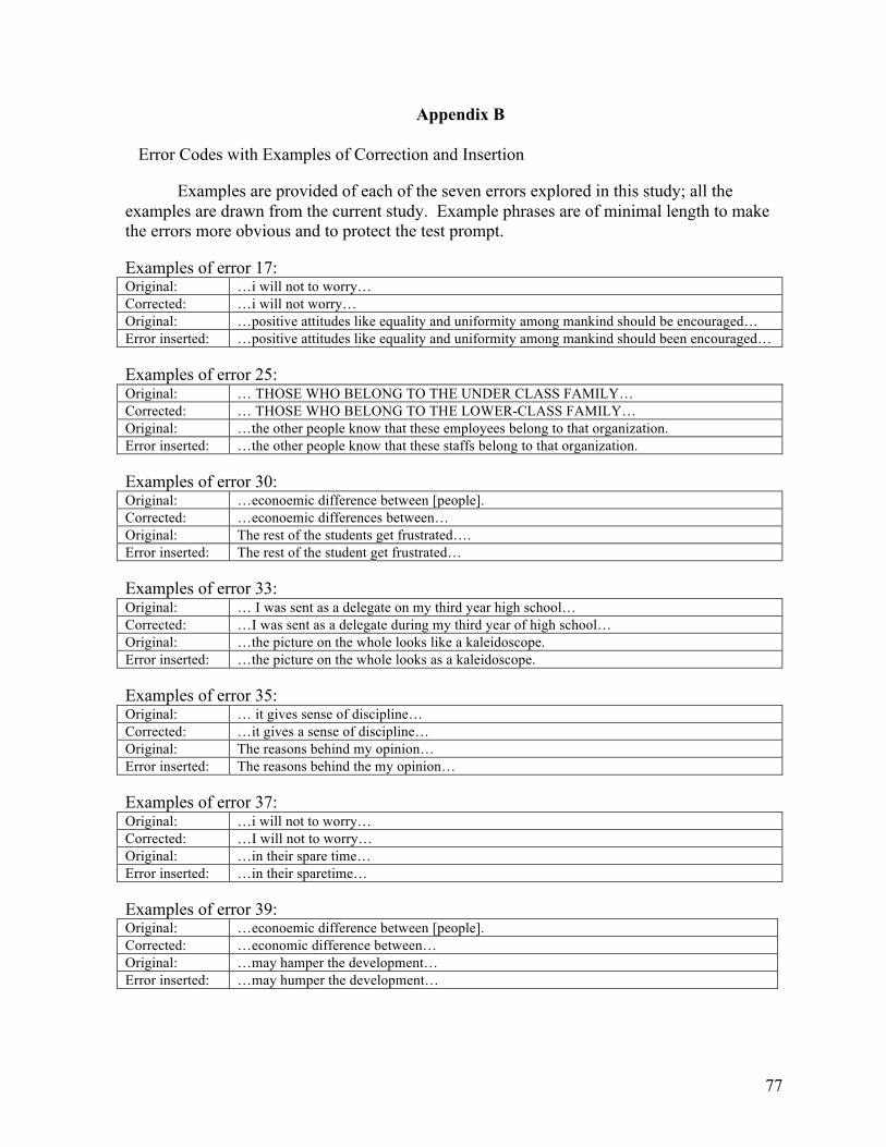
77

Appendix B Error Codes with Examples of Correction and Insertion

Examples are provided of each of the seven errors explored in this study; all the

examples are drawn from the current study. Example phrases are of minimal length to make the errors more obvious and to protect the test prompt.

Examples of error 17: Original: …i will not to worry… Corrected: …i will not worry… Original: …positive attitudes like equality and uniformity among mankind should be encouraged… Error inserted: …positive attitudes like equality and uniformity among mankind should been encouraged… Examples of error 25: Original: … THOSE WHO BELONG TO THE UNDER CLASS FAMILY… Corrected: … THOSE WHO BELONG TO THE LOWER-CLASS FAMILY… Original: …the other people know that these employees belong to that organization. Error inserted: …the other people know that these staffs belong to that organization. Examples of error 30: Original: …econoemic difference between [people]. Corrected: …econoemic differences between… Original: The rest of the students get frustrated…. Error inserted: The rest of the student get frustrated… Examples of error 33: Original: … I was sent as a delegate on my third year high school… Corrected: …I was sent as a delegate during my third year of high school… Original: …the picture on the whole looks like a kaleidoscope. Error inserted: …the picture on the whole looks as a kaleidoscope. Examples of error 35: Original: … it gives sense of discipline… Corrected: …it gives a sense of discipline… Original: The reasons behind my opinion… Error inserted: The reasons behind the my opinion… Examples of error 37: Original: …i will not to worry… Corrected: …I will not to worry… Original: …in their spare time… Error inserted: …in their sparetime… Examples of error 39: Original: …econoemic difference between [people]. Corrected: …economic difference between… Original: …may hamper the development… Error inserted: …may humper the development…

78

Appendix C Analytic Scoring Guide Adapted from English Language Institute, 1994.

Content Language 10 Topic is richly and fully developed.

Organization is appropriate and effective, and there is excellent control of connection. There is a wide range of vocabulary.

10 Flexible use of a wide range of syntactic (sentence level) structures, accurate morphological (word forms) control. Vocabulary is appropriately used. Spelling and punctuation appear error free.

9 Topic is fully and complexly developed. Organization is well controlled and appropriate to the material, and the writing is well connected. Vocabulary is broad.

9 Flexible use of a wide range of syntactic structures. Morphological control is nearly always accurate. Vocabulary is appropriately used. Spelling and punctuation errors are not distracting.

8 Topic is well developed, with acknowledgement of its complexity. Organization is controlled and generally appropriate to the material, and there are few problems with connection. Vocabulary is broad.

8 Varied syntactic structures are used with some flexibility, and there is good morphological control. Vocabulary is usually used appropriately. Spelling and punctuation errors are not distracting.

7 Topic is generally clearly and completely developed, with at least some acknowledgement of its complexity. Organization is controlled and shows some appropriateness to the material, and connection is usually adequate. Vocabulary use shows some flexibility.

7 Both simple and complex syntactic structures are generally adequately used; there is adequate morphological control. Vocabulary use is usually appropriate. Spelling and punctuation errors are sometimes distracting.

6 Topic is developed clearly but not completely and without acknowledging its complexity. Organization is generally controlled, while connection is sometimes absent or unsuccessful. Vocabulary is adequate.

6 Both simple and complex syntactic structures are present; in some "6 language" essays these are cautiously and accurately used while in others there is more fluency and less accuracy. Morphological control is inconsistent. Vocabulary may sometimes be inappropriately used. Spelling and punctuation errors are sometimes distracting.

5 Topic development is present, although limited by incompleteness, lack of clarity, or lack of focus. The topic may be treated as though it has only one dimension, or only one point of view is possible. Organization is partially controlled, while connection is often absent or unsuccessful. Vocabulary is sometimes inadequate.

5 In some "5 language" essays both simple and complex syntactic structures are present, but with many errors; others have accurate syntax but are very restricted in the range of language attempted. Morphological control is inconsistent. Vocabulary is sometimes inappropriately used. Spelling and punctuation errors are sometimes distracting.

79

4 Topic development is present but restricted, and often incomplete or unclear. Organization, when apparent, is poorly controlled, and little or no connection is apparent. Narrow and simple vocabulary usually approximates meaning.

4 Simple syntactic structures dominate, with many errors; complex syntactic structures, if present, are not controlled. Lacks morphological control. Vocabulary is often inappropriately used. Spelling and punctuation errors are often distracting.

3 Contains little sign of topic development. There is little or no organization, and no connection apparent. Vocabulary is narrow and simple.

3 Simple syntactic structures are present, but with many errors; lacks morphological control. Inappropriate vocabulary inhibits communication, and spelling and punctuation errors often cause serious interference.

2 Contains only fragmentary communication about the topic. No organization or connection are apparent. Vocabulary is highly restricted.

2 There is little syntactic or morphological control. Vocabulary is inaccurately used. Spelling is often indecipherable and punctuation is missing or appears random.

1 Communicates nothing, and is often copied directly from the prompt. No apparent organization or connection. Vocabulary is extremely restricted and repetitively used.

1 There is little sign of syntactic or morphological control. Vocabulary is inaccurately used. Spelling is often indecipherable and punctuation is missing or appears random.

The following exceptional aspects may affect the score, if the rater determines that that aspect is so well/poorly written as to add significantly to or detract significantly from the overall content or language of the essay: Increase content score by 1: • topic especially well developed • organization especially well controlled • connection especially smooth • vocabulary especially broad

Increase language score by 1: • syntactic structures especially complex • especially good morphological control

Decrease content score by 1: • topic especially poorly or incompletely

developed • organization especially uncontrolled • connection especially poor • vocabulary especially narrow • question misinterpreted or not addressed

Decrease language score by 1: • syntactic (sentence level) structures especially

simple • syntactic structures especially uncontrolled • especially poor morphological (word forms)

control • vocabulary use especially inappropriate • spelling especially inaccurate • punctuation especially inaccurate • paragraph divisions missing or apparently

random

80

Appendix D Percentage of Comments by Type

Classification scheme adapted from Cumming, Kantor, and Powers (2002). All of Cumming, Kantor, and Powers’ categories are listed, with one new Self-Monitoring Focus category, “Consider or interpret descriptors on the analytic scale,” added for this study.

Decision Making Behaviors

Percentage of total comments by all three raters of 2016 coded comments on 180 essays

Percentage of total comments by all raters of 1561 coded comments on 180 essays (Scoring decisions omitted)

Percentage of comments by rater 1 of 381 coded comments on 60 essays (Scoring decisions omitted)

Percentage of comments by rater 2 of 675 coded comments on 60 essays (Scoring decisions omitted)

Percentage of comments by rater 3 of 505 coded comments on 60 essays (Scoring decisions omitted)

Comment contain-ing example (Appen-dix E)

Classi-fication code

Self-Monitoring Focus 33.73 14.41 19.16 17.78 6.34 Interpretation Strategies Read or interpret essay prompt 0.10 0.13 0.00 0.15 0.20 a I1 Read or reread composition 3.32 4.29 6.56 5.03 1.58 b, q, w I2 Envision personal situation of the writer

0.74 0.96 0.26 0.59 1.98 c, n I3

Scan whole composition 1.49 1.92 2.10 3.26 0.00 d I4 Judgment Strategies Decide on macrostrategy for reading and rating

0.00 0.00 0.00 0.00 0.00 None J1

Consider own personal response or biases

0.45 0.58 1.31 0.30 0.40 e, f, g, s J2

Consider or interpret descriptors on the analytic scale

2.43 3.14 4.46 4.00 0.99 g, i J8

Define or revise own criteria 0.00 0.00 0.00 0.00 0.00 None J3 Compare with other compositions or "anchors"

0.84 1.09 1.57 0.89 0.99 e, v J4

Summarize, distinguish, or tally judgments collectively

0.00 0.00 0.00 0.00 0.00 None J5

Articulate general impressions 1.79 2.31 2.89 3.56 1.98 e, m J6 Articulate or revise scoring decision 22.57 X X X X h, m, q, z J7 Rhetorical and Ideational Focus 31.30 40.42 31.76 41.78 45.15 Interpret ambiguous or unclear phrases 0.25 0.32 0.26 0.59 0.00 b, w R1 Discern rhetorical structure 1.34 1.79 1.31 2.67 0.99 j, q R2 Summarize ideas or propositions 1.49 1.92 0.52 2.96 1.58 k, q R3 Assess reasoning, logic, or topic development

8.58 11.08 7.87 9.63 15.44 a, i R4

Assess task completion 0.35 0.45 0.78 0.00 0.79 l R5 Assess relevance 0.35 0.45 0.26 0.30 0.79 m R6 Assess coherence 4.71 6.09 7.35 5.48 5.94 n R7 Assess interest, originality, or creativity

0.60 0.77 0.26 1.48 0.20 o R8

Identify redundancies 0.74 0.96 1.31 0.89 0.79 p R9 Assess text organization 7.24 9.35 4.99 10.07 11.68 j, k R10 Assess style, register, or genre 2.13 2.75 2.62 3.56 1.78 q R11 Rate ideas or rhetoric 3.47 3.47 4.48 4.20 5.15 r R12 Language Focus 34.92 45.10 48.82 40.44 48.52 Observe layout 0.05 0.06 0.26 0.00 0.00 s L1 Classify errors into types 3.72 4.80 3.67 5.33 4.95 t, x L2 Edit phrases for interpretation 0.35 0.45 0.26 0.89 0.0 u L3 Assess quantity or total written production

0.40 0.51 0.79 0.30 0.59 v L4

Assess comprehensibility 3.17 4.10 7.35 2.67 3.56 w L5 Consider gravity of errors 1.98 2.56 1.31 2.52 3.56 y L6 Consider error frequency 2.48 3.20 2.62 4.30 2.18 t L7 Assess fluency 1.29 1.67 0.79 1.93 1.98 z L8 Consider lexis 7.74 9.99 9.97 9.04 11.29 t, y L9 Consider syntax or morphology 6.70 8.65 16.27 4.89 7.92 d, t L10 Consider spelling or punctuation 0.94 1.22 1.05 1.93 0.40 u L11 Rate language overall 6.10 7.88 4.46 6.67 12.08 d L12

81

Appendix E Examples of Rater Commentary, with Classification Codes

The examples below of comments taped by the raters show how comment types were classified.

Classification codes in gray correspond to the categories derived from Cumming, Kantor, and Powers (2003) as shown in Appendix D. Each classification code corresponds to one of the total of 2016 comments classified. Where the same code appears twice, two separate comments of a type were counted; where a code appears once, one instance of that category was counted. Where the rater was reading aloud from a composition, only the first three words read from the composition appear, in single quotes.

a. “I started thinking that, considering what the topic is, considering that the topic is [summary of topic]I1, I thought that it was well developed.R4”

b. “The second from the last paragraph: ‘Sometimes students are…’I2 Now I can figure out what they mean,R1 but that’s kind of one of those moments you have to decipher.L5”

c. “That, I mean it’s, maybe he ran out of time, I don’t know I3.” d. “Syntax is really bad. L10 You look at paragraph 3, sentence 1, paragraph 4, paragraph 6I4. It [the

essay]’s very weak.L12” e. “It’s getting really tough to read these.J2 These seem just like miserable essaysJ6, very much lower

than the ones I’ve been reading latelyJ4. For real.” f. “There’s just things in here—I just, it doesn’t ring true.J2 You don’t see people do this.” g. “At this point in reading, I discovered I’m having a really hard time with the content scale. I can’t tell

the difference in the descriptors of a 5 and a 6.J8 It’s, um, not the way I’m used to looking at these kinds of impromptu compositions.J2”

h. “For language, I was going back and forth between giving it a 6 and 7, a 6 and a 7.J7” i. “It [the analytic scale] saysJ8 that the topic is developed clearlyR4 but not completelyR4, and that’s

certainly the case in composition number 25162. The reasons that she gives are stated, but not developed.”

j. “It seems more or less organized.R10 There’s sort of an introduction, they develop positive things, and they mention the negative things, and then we saw a conclusion.R2”

k. “It seemed there was an organization to itR10. He kind of tried to tie in this whole idea of, you know there’s a race, and getting, if you spend all of your energy on one thing, you won’t be able to get to the academic stuffR3, so, you know, it was sort of a little bit different approachR10.”

l. “…but you know, I mean, there is an argument present here that I can seeR5.” m. “It goes off-topic in spots,R6 and the language is 2 also.J7 It’s an extremely weak essayJ6.” n. “They were kind of just used almost like the student learnedI3 you’re supposed to start your sentences

with these transition wordsR7.” o. “It’s nice to see it, the essay, to see it developed in sort of a different way…R8” p. “That’s just sort of repetitious.R9” q. “I give it a 4 for content.J7 It’s really more description than argument,R11 and a 3 for language.J7 I

guess there’s a little bit of an argumentR2: ‘One student will ….’I2 That idea that you can identify students,R3 but still it’s mostly description,R11 so I’m going to stick with that 4.J7”

r. “They do have kind of a nice exampleR12 of the college students…” s. “I’m having trouble…I’m used to reading compositions handwrittenJ2, and I’m not sure how the effect

of seeing these typedL1 is affecting my judgment of how frequent errors are in the whole picture of a composition.”

t. “There are manyL7 errors in syntaxL10, morphologyL10, vocabularyL9, unclear referenceL2 in that first paragraph…”

u. “There was a comma after the word ‘levels’ that sort of threw me L11. Without the comma, the sentence makes senseL3.”

v. “This one’s noticeably weaker than the others.J4 It seems a bit short.L4” w. “The second from the last paragraph: ‘Sometimes students are…’I2 Now I can figure out what they

mean,R1 but that’s kind of one of those moments you have to decipher.L5” x. “There’s some problems with verb tenses…L2” y. “The vocabulary seemed fineL9. ‘Cloth’ instead of ‘clothes,’ but it didn’t really get in the wayL6.” z. “This one seemed pretty straightforward 6 levelJ7…You know, rather fluentL8…”

82

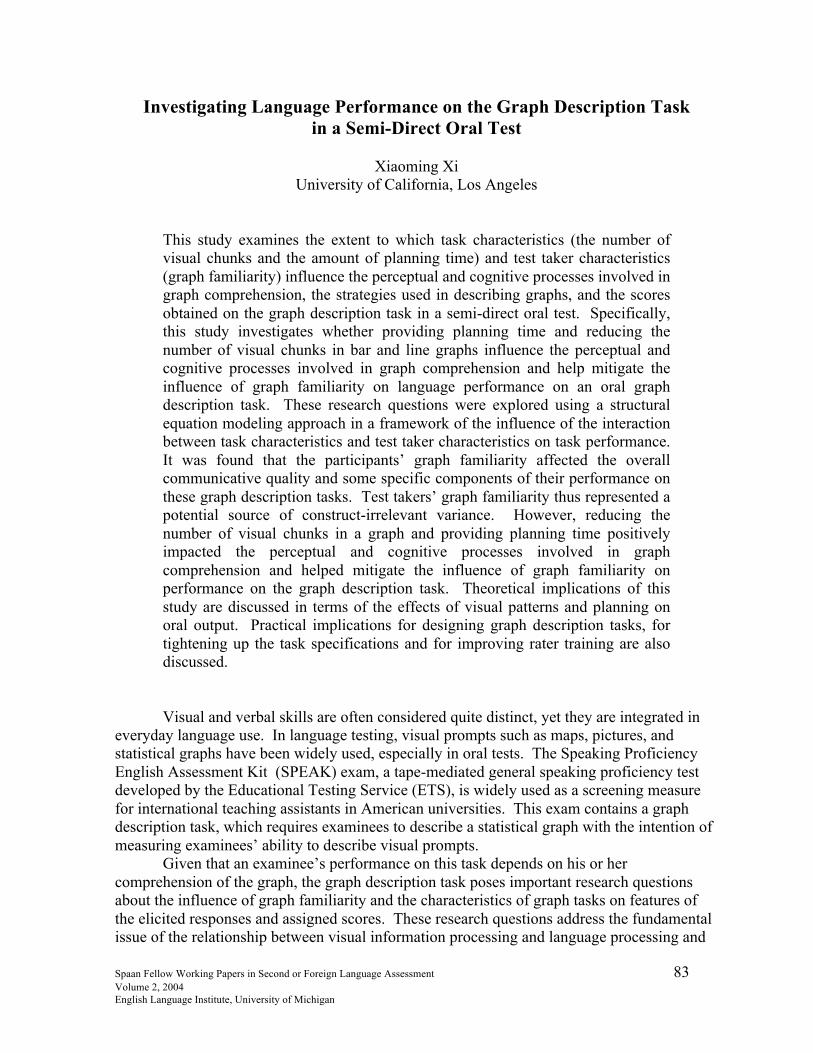
Spaan Fellow Working Papers in Second or Foreign Language Assessment 83 Volume 2, 2004 English Language Institute, University of Michigan

Investigating Language Performance on the Graph Description Task in a Semi-Direct Oral Test

Xiaoming Xi

University of California, Los Angeles This study examines the extent to which task characteristics (the number of visual chunks and the amount of planning time) and test taker characteristics (graph familiarity) influence the perceptual and cognitive processes involved in graph comprehension, the strategies used in describing graphs, and the scores obtained on the graph description task in a semi-direct oral test. Specifically, this study investigates whether providing planning time and reducing the number of visual chunks in bar and line graphs influence the perceptual and cognitive processes involved in graph comprehension and help mitigate the influence of graph familiarity on language performance on an oral graph description task. These research questions were explored using a structural equation modeling approach in a framework of the influence of the interaction between task characteristics and test taker characteristics on task performance. It was found that the participants’ graph familiarity affected the overall communicative quality and some specific components of their performance on these graph description tasks. Test takers’ graph familiarity thus represented a potential source of construct-irrelevant variance. However, reducing the number of visual chunks in a graph and providing planning time positively impacted the perceptual and cognitive processes involved in graph comprehension and helped mitigate the influence of graph familiarity on performance on the graph description task. Theoretical implications of this study are discussed in terms of the effects of visual patterns and planning on oral output. Practical implications for designing graph description tasks, for tightening up the task specifications and for improving rater training are also discussed. Visual and verbal skills are often considered quite distinct, yet they are integrated in

everyday language use. In language testing, visual prompts such as maps, pictures, and statistical graphs have been widely used, especially in oral tests. The Speaking Proficiency English Assessment Kit (SPEAK) exam, a tape-mediated general speaking proficiency test developed by the Educational Testing Service (ETS), is widely used as a screening measure for international teaching assistants in American universities. This exam contains a graph description task, which requires examinees to describe a statistical graph with the intention of measuring examinees’ ability to describe visual prompts.

Given that an examinee’s performance on this task depends on his or her comprehension of the graph, the graph description task poses important research questions about the influence of graph familiarity and the characteristics of graph tasks on features of the elicited responses and assigned scores. These research questions address the fundamental issue of the relationship between visual information processing and language processing and

84

production and the more practical issue of the validity of using visuals in language assessments. These questions can be explored in the framework of the interaction of task characteristics and test taker characteristics on test performance. However, despite the abundance of literature in language testing on how task characteristics and test taker characteristics affect test performance, there are very few studies addressing the role of visual information and the relationship between visual cues and performance in language testing (for exceptions, see Ginther, 2001; Gruba, 1997; 1999). Moreover, these studies that investigate the influence of visual information on test performance have generally been conducted in the context of listening assessments.

In recent years, there has been considerable research in cognitive psychology into how humans perceive, process and understand statistical displays, and extensive work on spontaneous verbal interpretations of graphs by native speakers of English (Carpenter & Shah, 1998; Carswell, 1993; Carswell, Bates, Pregliasco, Lonon, & Urban, 1998; Carswell & Ramzy, 1997; Kosslyn, 1989; Pinker, 1990; Peebles, Cheng & Shaboldt, 2000; Shah & Carpenter, 1995). This body of literature illuminates this study, especially in terms of the cognitive processes involved in graph comprehension and interpretation and the kinds of graph features that might influence comprehension and interpretation.

The major graph comprehension frameworks in cognitive psychology see graph comprehension as an interaction of bottom-up perceptual and top-down cognitive processes (Peebles, et al, 2000; Pinker, 1990). Therefore, both graph reading schemata (top-down) and perceptual features (bottom-up) of the graph play roles in graph comprehension.

On the cognitive side, one’s graph reading schema guides the processes of information locating, retrieving, and integration. Some people are sophisticated graph readers and some are novices. The amount of training and experience in the use of graphs may be related to the content and sophistication of the interpretation. However, graph familiarity is not defined as part of the construct of the graph description task in the SPEAK, so clearly it represents a potential source of construct-irrelevant variance.

On the perceptual side, the graph viewer has to rely solely on the visual information in the graph to comprehend and interpret it. Graphs should be designed so as to minimize the amount of integration and inference that needs to be made by the graph viewer and to facilitate interpretations based on the Gestalt principles such as proximity and continuity (Peebles, et al, 2000; Shah, Hegarty, & Mayer, 1999).

The research on visual information organization in graphs and perception and processing of graphs has been guided by the Gestalt principles (Carswell, Emery, & Lonon, 1993; Carswell, et al., 1998; Carswell & Ramzy, 1997; Shah, Hegarty & Mayer, 1999). The relevant Gestalt principles are proximity, continuity and similarity. The principle of proximity states that things close together are perceived as a chunk. The principle of continuity predicts the preference for continuous figures. The principle of similarity states that things which share visual characteristics such as shape, size, color, or texture will be seen as belonging together. Therefore, bars that are grouped together might form the visual chunks in bar graphs (Shah, et al, 1999), whereas separate lines or line segments constitute visual chunks in line graphs (Carswell, et al, 1993).

In earlier collaborative studies (Katz, Xi, Kim, Cheng, in press; Xi, 2002), we looked at how the number of visual chunks in bar graphs and the prompt type affected the communicative quality of the elicited responses to some experimental bar graph tasks, comparing examinees’ scores across bar graph tasks with varying numbers of visual chunks

85

and different prompt types. The few-chunk and many-chunk graphs were created by reversing the variables on the X axis, and the prompts included the generic prompt (“Describe the information in the graph”) and the direct and explicit prompt (“Tell us the changes from year x to year y”).

The results indicated that when the major points were packaged in relatively fewer visual chunks, more sophisticated language functions such as global comparisons and trend descriptions were produced, which in turn were perceived by the raters as more developed responses and superior performances. Another important finding was that the examinees spent significantly less time studying the few-chunk graphs and planning their responses, suggesting that few-chunk graphs might have been perceived as less complex compared to the many-chunk graphs.

This difference in performance was only seen when a graph was processed online with no planning time provided and under the one-minute response time constraint, with the examinees biased toward describing the quantitative information represented in the visual chunks. If some planning time were given, we might expect the examinees to be driven more by analytical thinking and integration of the information instead of the perceptual features, and see a difference in their choices of descriptive strategies. The planning time provided might also help mitigate the influence of one’s graph familiarity. Therefore, in this current study, the experimental bar graph items differed not only in the number of visual chunks but also in whether planning time was provided.

This additional variable of planning time is being used to explore the following questions: Overall, will the planning time provided facilitate graph comprehension and performance on the graph task? Specifically, when no specific planning time is provided, will it compensate for the amount of time spent during online processing in integrating information in the many-chunk graph and lead to interpretations of better communicative quality?

In addition to comparing performances across bar graphs, which were essentially different representations of the same data, this study also attempts to evaluate the communicative quality of spontaneous interpretations of line graphs that shared the same story line but represented different quantitative information. According to Carswell, et al. (1993), each trend change, not a data point, represents a visual chunk in a line graph. This study looks at line graphs with few and many visual chunks. It investigates whether the influence of the number of visual chunks is the same across the two most commonly used graph formats in the SPEAK exam, bar graphs, and line graphs.

The overarching research question is whether task characteristics (graph display and the amount of planning time provided) and test takers’ graph familiarity have any influence on the perceptual and cognitive processes involved in graph comprehension, graph description strategies, and performance on graph tasks. The specific research questions are stated below:

1. To what extent do examinees’ description strategies tend to differ across bar and line graph tasks with varying numbers of visual chunks and amount of planning time?

2. To what extent do examinees’ responses to bar graph and line graph tasks with different numbers of visual chunks and amount of planning time tend to get different holistic scores? Is the influence of the number of visual chunks and planning time the same across the bar and line graph tasks?

86

3. To what extent do the number of visual chunks and the amount of planning time influence examinees’ analytical scores on the bar graph and line graph tasks? Is the influence of the number of visual chunks and planning time the same across the bar and line graph tasks?

4. To what extent does examinees’ graph familiarity influence their performance on the graph tasks? Is the influence of graph familiarity the same across the bar and line graph tasks?

Literature Review

Studies on Graph Comprehension Underlying the graph comprehension work are a plethora of cognitive models which

attempt to account for the processes involved in graph comprehension and factors influencing graph comprehension, among which are the graph-reading knowledge of the person (Pinker, 1990), visual characteristics of the graph, (Carpenter & Shah, 1998; Carswell, et al, 1993; Carswell, et al., 1998; Kosslyn, 1989; Peebles, et al, 2000; Shah & Carpenter, 1995) and task features (Peebles, et al, 2000; Pinker, 1990). Cognitive Processes Involved in Graph Comprehension

Carpenter and Shah’s model (Carpenter & Shah, 1998; Shah, 1995; Shah & Carpenter, 1995) discusses three cognitive processes that graph viewers are engaged in during graph comprehension: 1) detecting and encoding the visual patterns; 2) identifying the quantitative relationships that those visual features represent; and 3) relating those quantitative relations to the variables. The first two processes are focused on during the discussion of how quantitative relationships are packaged in visual chunks. Top-Down and Bottom-Up Processes

Pinker’s (1990) cognitive framework for graph comprehension emphasizes the interaction of perceptual data-driven (bottom-up) and cognitive schema-driven (top-down) processing, with the top-down component guiding attention and perception involved in the bottom-up processing. His model specifies in great detail the knowledge structure of the graph user and how this knowledge guides graph comprehension. His model also recognizes that both the type of graph and the type of task affect graph comprehension, the former affecting the graph encoding process and the latter driving the information retrieval process. However, one of the limitations of Pinker’s model is that it discusses graph reading schemata merely in terms of graph types, ignoring the differences in graph schemata applied to graphs that are of the same type but differ in other dimensions.

Peebles, et al. (2000) propose a very comprehensive graph-based reasoning (GBR) model. This model elaborates on the variables that interact to affect the speed and accuracy of users’ problem solving behavior with a specific graph and task, and the processes involved. It defines graph comprehension as a function of the graph reading schemata of viewers, the properties of the graph such as the type of graph being used and the visual-spatial patterns present in the graph, and the specific task that the user attempts to accomplish. The GBR model also specifies three dimensions involved: the general and specific graph knowledge possessed by the user, the visual properties of the graph, and the amount of external and visual search and internal mental inference that are performed by the graph viewer. Although

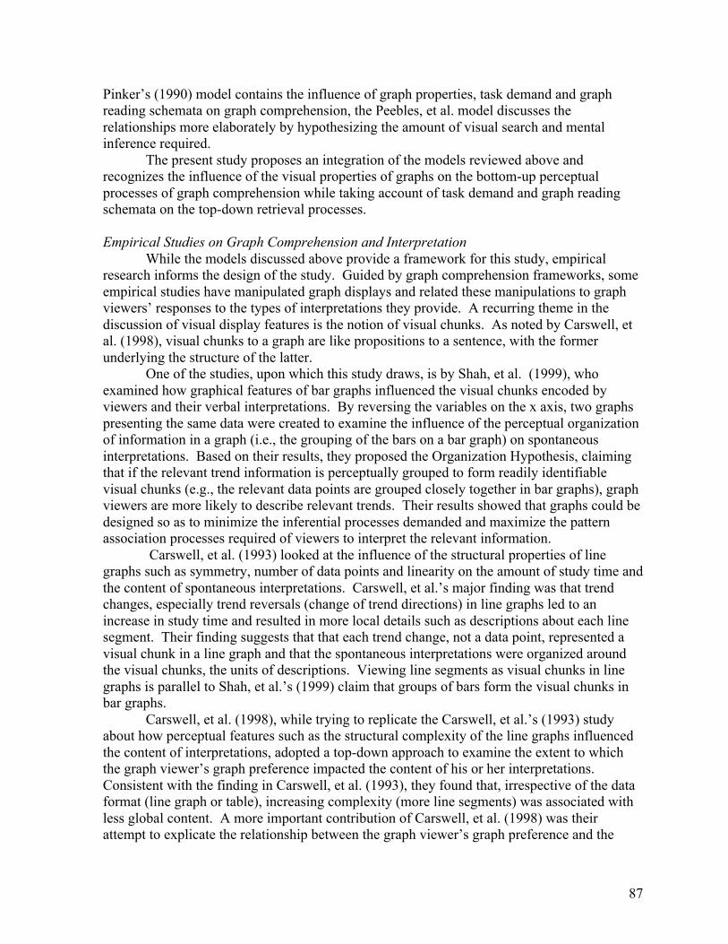
87

Pinker’s (1990) model contains the influence of graph properties, task demand and graph reading schemata on graph comprehension, the Peebles, et al. model discusses the relationships more elaborately by hypothesizing the amount of visual search and mental inference required.

The present study proposes an integration of the models reviewed above and recognizes the influence of the visual properties of graphs on the bottom-up perceptual processes of graph comprehension while taking account of task demand and graph reading schemata on the top-down retrieval processes. Empirical Studies on Graph Comprehension and Interpretation

While the models discussed above provide a framework for this study, empirical research informs the design of the study. Guided by graph comprehension frameworks, some empirical studies have manipulated graph displays and related these manipulations to graph viewers’ responses to the types of interpretations they provide. A recurring theme in the discussion of visual display features is the notion of visual chunks. As noted by Carswell, et al. (1998), visual chunks to a graph are like propositions to a sentence, with the former underlying the structure of the latter.

One of the studies, upon which this study draws, is by Shah, et al. (1999), who examined how graphical features of bar graphs influenced the visual chunks encoded by viewers and their verbal interpretations. By reversing the variables on the x axis, two graphs presenting the same data were created to examine the influence of the perceptual organization of information in a graph (i.e., the grouping of the bars on a bar graph) on spontaneous interpretations. Based on their results, they proposed the Organization Hypothesis, claiming that if the relevant trend information is perceptually grouped to form readily identifiable visual chunks (e.g., the relevant data points are grouped closely together in bar graphs), graph viewers are more likely to describe relevant trends. Their results showed that graphs could be designed so as to minimize the inferential processes demanded and maximize the pattern association processes required of viewers to interpret the relevant information.

Carswell, et al. (1993) looked at the influence of the structural properties of line graphs such as symmetry, number of data points and linearity on the amount of study time and the content of spontaneous interpretations. Carswell, et al.’s major finding was that trend changes, especially trend reversals (change of trend directions) in line graphs led to an increase in study time and resulted in more local details such as descriptions about each line segment. Their finding suggests that that each trend change, not a data point, represented a visual chunk in a line graph and that the spontaneous interpretations were organized around the visual chunks, the units of descriptions. Viewing line segments as visual chunks in line graphs is parallel to Shah, et al.’s (1999) claim that groups of bars form the visual chunks in bar graphs.

Carswell, et al. (1998), while trying to replicate the Carswell, et al.’s (1993) study about how perceptual features such as the structural complexity of the line graphs influenced the content of interpretations, adopted a top-down approach to examine the extent to which the graph viewer’s graph preference impacted the content of his or her interpretations. Consistent with the finding in Carswell, et al. (1993), they found that, irrespective of the data format (line graph or table), increasing complexity (more line segments) was associated with less global content. A more important contribution of Carswell, et al. (1998) was their attempt to explicate the relationship between the graph viewer’s graph preference and the

88

grainsize of his or her interpretation. They found that the amount of global and local content did not differ as a function of the graph viewer’s graph preference. However, they claimed that the group scoring low for graph preference tended to report more point values, despite that fact that the difference in point value reporting behavior across the two groups was not very reliable and was prone to chance, as indicated by the relevant p value (= .058) reported in their study. The results of this study seem to suggest that graph complexity was the predominant factor affecting the content of spontaneous interpretations and that the graph viewer’s graph preference had minimal influence. However, this could be due to the nature of the graph preference questionnaire used in this study. This questionnaire attempted to elicit the graph viewer’s typical reactions to graphs, which represents only one dimension of the graph-reading schema of the graph viewer. Other measures should be designed so as to form a composite measure to evaluate the graph viewer’s experience with graphs, familiarity with graphs, and ability to read graphs. This composite measure could potentially be a more sensitive measure of the graph reading background variable that the authors were interested in.

The present study draws heavily on the notion of visual chunks in bar graphs as discussed in Shah, et al. (1999), and in line graphs as examined in Carswell, et al. (1993) and Carswell, et al. (1998). The review of the studies above from a cognitive psychology perspective helps fill the vacuum in the research of using statistical graphs in oral tests and pinpoints the graph characteristics and graph viewer characteristics that might be of interest to the present study. The next section reviews studies that address the effect of planning time on qualities of elicited oral discourse in second language acquisition and testing, since planning time was a major manipulation in this study. Effect of Planning Time on Speech Production in Second Language Acquisition and Testing

Most of the studies on planning have been conducted in the context of second language (L2) variability and planning has been considered as one of the factors that might account for the variability in L2 oral production. As noted by Ellis (1994), L2 speech production is not always automatic and goes through a series of processing stages. Therefore, the oral output is likely to be affected by the amount of time available for planning. Butterworth (1980) states that planning consists of macro- and micro-planning, the former involving planning big chunks of discourse in terms of semantic and syntactic organization and the latter concerning the monitor of local functions such as word choices and clause boundary markings (p. 159). However, it remains fuzzy as to what aspects of the oral output are subject to the influence of planning.

Some studies have found that the oral discourse elicited under planning conditions showed greater complexity (Crookes, 1989; Foster & Skehan, 1996) and fluency (Foster & Skehan, 1996; Mehnert, 1998); however, there have been conflicting findings on the influence of planning on accuracy (Crookes, 1989; Ellis, 1987; Foster & Skehan, 1996; Mehnert, 1998). Skehan (1998) proposed the limited processing capacity theory to explain the conflicting findings. He argued that L2 learners cannot allocate their limited attention to all aspects of oral production and that the learners’ decision on which components to channel resources to depends on what they choose or are instructed to prioritize.

In the studies on the effect of planning time on oral output in second language acquisition, the tasks used provided ample planning time (usually ten minutes) and were not

89

contextualized in testing environments. Wigglesworth (1995) explored the necessity of providing planning time for speaking tasks in semi-direct oral tests and conducted one of the first studies that examined the impact of minimal planning time on examinee discourse in testing conditions. A major finding in this study was that examinees’ oral discourse was more accurate on the more difficult tasks under the one-minute planning time condition.

In another attempt to look at the same data, Wigglesworth (1997) compared the planned and unplanned discourse on several tasks that differed in their difficulty levels in complexity, accuracy, and fluency across the high- and low-proficiency groups. The results of the linguistic analyses revealed that high-proficiency speakers demonstrated superior oral discourse under the planned condition, as reflected by higher complexity, better fluency and increased accuracy, but the benefit of planning was manifest on only the more difficult tasks. In contrast, the low-proficiency speakers did not seem to have gained much advantage by the presence of planning time.

Motivated by Skehan’s work on factors that affect task difficulty, Wigglesworth (2001) used speaking tasks that differed in task characteristics including structure and familiarity of activity performed under planned (five minutes planning time) or unplanned test conditions. Then these task characteristics were related to the difficulty levels of the tasks. The results pointed to the conclusion that a task that represented familiar activity was easier when planning time was not available. Moreover, planning time had a negative influence on test scores on both structured and unstructured tasks. These results were counter-intuitive; however, they might be attributable to the nature of the analytic scale used, which had four components: grammar, fluency, cohesion and communicative effectiveness. Wigglesworth speculated that the planning time available encouraged the test takers to be more ambitious with the language and to produce more complex language, which in turn made them falter or hurt the accuracy of their language. These negative consequences might have been reflected in the fluency and accuracy ratings.

Planning time was also one of the performance conditions manipulated in Iwashita, McNamara, & Elder (2001), which investigated how varying task dimensions and performance conditions were related to the task difficulty of narrative tasks based on a set of pictures in a semi-direct oral test. This study attempted to operationalize the cognitive variables that affect oral task difficulty discussed in the work of Skehan and Robinson (Skehan, 1996, 1998; Robinson, 1995, 1996, 2001, and 2003). Contrary to the prediction that more planning time would make the narrative task easier, the analysis on the assigned ratings showed that planning time was not related to task difficulty significantly. The linguistic analyses also showed that the oral discourse elicited under the two planning conditions did not differ significantly in fluency, accuracy or complexity. However, as noted by the authors themselves, more planning time on more complex narrative tasks might have increased fluency and accuracy of the elicited discourse. Another explanation might be that during the planning phase, the test takers channeled their attention-related resources to other aspects of their language performance, such as content, and the effect of planning may not have been manifest in fluency or accuracy.

In this study, the planning time provided could be used for both studying the graphs and planning a certain portion of the discourse. The studies reviewed in this section are informative, but the effect of planning time might play out in somewhat different ways.

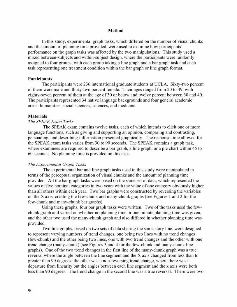
90

Method

In this study, experimental graph tasks, which differed on the number of visual chunks and the amount of planning time provided, were used to examine how participants’ performance on the graph tasks was affected by the two manipulations. This study used a mixed between-subjects and within-subject design, where the participants were randomly assigned to four groups, with each group taking a line graph and a bar graph task and each task representing one treatment condition within the bar graph or line graph format. Participants

The participants were 236 international graduate students at UCLA. Sixty-two percent of them were male and thirty-two percent female. Their ages ranged from 20 to 49, with eighty-seven percent of them at the age of 30 or below and twelve percent between 30 and 40. The participants represented 34 native language backgrounds and four general academic areas: humanities, social sciences, sciences, and medicine. Materials The SPEAK Exam Tasks

The SPEAK exam contains twelve tasks, each of which intends to elicit one or more language functions, such as giving and supporting an opinion, comparing and contrasting, persuading, and describing information presented graphically. The response time allowed for the SPEAK exam tasks varies from 30 to 90 seconds. The SPEAK contains a graph task, where examinees are required to describe a bar graph, a line graph, or a pie chart within 45 to 60 seconds. No planning time is provided on this task. The Experimental Graph Tasks

The experimental bar and line graph tasks used in this study were manipulated in terms of the perceptual organization of visual chunks and the amount of planning time provided. All the bar graph tasks were based on the same set of data, which represented the values of five nominal categories in two years with the value of one category obviously higher than all others within each year. Two bar graphs were constructed by reversing the variables on the X axis, creating the few-chunk and many-chunk graphs (see Figures 1 and 2 for the few-chunk and many-chunk bar graphs).

Using these graphs, four bar graph tasks were written. Two of the tasks used the few-chunk graph and varied on whether no planning time or one minute planning time was given, and the other two used the many-chunk graph and also differed in whether planning time was provided.

Two line graphs, based on two sets of data sharing the same story line, were designed to represent varying numbers of trend changes, one being two lines with no trend changes (few-chunk) and the other being two lines, one with two trend changes and the other with one trend change (many-chunk) (see Figures 3 and 4 for the few-chunk and many-chunk line graphs). One of the two trend changes in the first line of the many-chunk graph was a true reversal where the angle between the line segment and the X axis changed from less than to greater than 90 degrees; the other was a non-reversing trend change, where there was a departure from linearity but the angles between each line segment and the x axis were both less than 90 degrees. The trend change in the second line was a true reversal. There were two

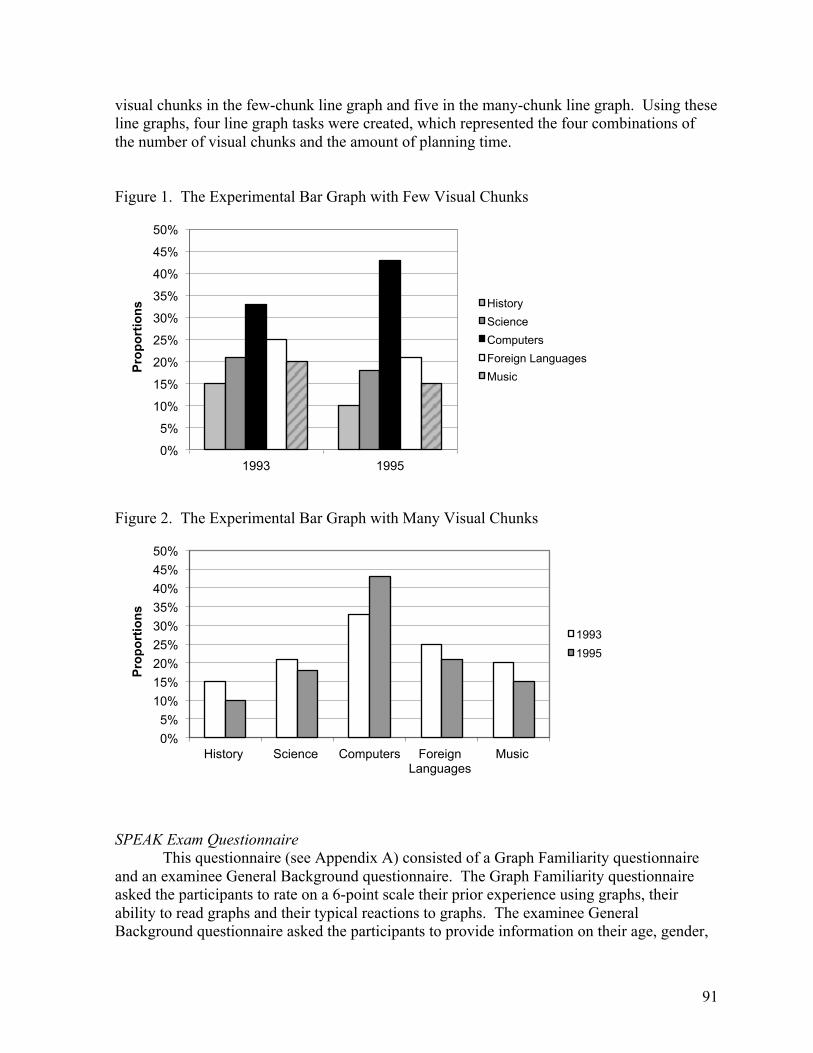
91

visual chunks in the few-chunk line graph and five in the many-chunk line graph. Using these line graphs, four line graph tasks were created, which represented the four combinations of the number of visual chunks and the amount of planning time. Figure 1. The Experimental Bar Graph with Few Visual Chunks

Figure 2. The Experimental Bar Graph with Many Visual Chunks

SPEAK Exam Questionnaire

This questionnaire (see Appendix A) consisted of a Graph Familiarity questionnaire and an examinee General Background questionnaire. The Graph Familiarity questionnaire asked the participants to rate on a 6-point scale their prior experience using graphs, their ability to read graphs and their typical reactions to graphs. The examinee General Background questionnaire asked the participants to provide information on their age, gender,

0%

5%

10%

15%

20%

25%

30%

35%

40%

45%

50%

1993 1995

Prop

ortio

ns History

Science Computers Foreign Languages Music

0% 5%

10% 15% 20% 25% 30% 35% 40% 45% 50%

History Science Computers Foreign Languages

Music

Prop

ortio

ns

1993 1995

92

native language, major (undergraduate and graduate), etc. This questionnaire was revised on the basis of the background questionnaire that was used in earlier collaborative studies (Katz, et al., in press; Xi, 2002) and the graph preference questionnaire used in Carswell, et al. (1998).

Figure 3. The Experimental Line Graph with Few Visual Chunks

Figure 4. The Experimental Line Graph with Many Visual Chunks

Procedure The experimental graph tasks were administered during three regular SPEAK exam administrations at UCLA, following the routine SPEAK exam sessions. Following human

0

1000

2000

3000

4000

5000

6000

7000

Apr. May. Jun. Jul. Aug. Sep.

# of

vis

itors

per

day

Month

average number of visitors per day in two cities

American city Australian city

0

1000

2000

3000

4000

5000

6000

7000

May

Jun. Jul. Aug. Sep. Oct.

# of

vis

itors

per

day

Month

average number of visitors per day in two cities

American city Australian city

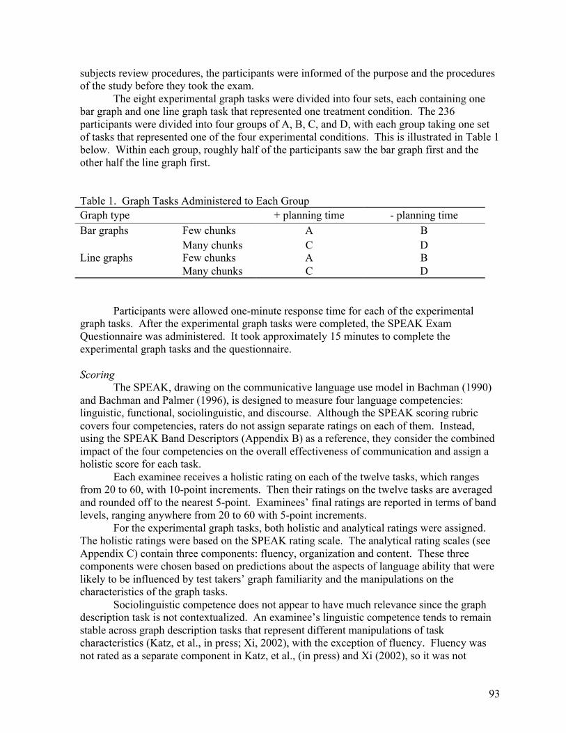
93

subjects review procedures, the participants were informed of the purpose and the procedures of the study before they took the exam.

The eight experimental graph tasks were divided into four sets, each containing one bar graph and one line graph task that represented one treatment condition. The 236 participants were divided into four groups of A, B, C, and D, with each group taking one set of tasks that represented one of the four experimental conditions. This is illustrated in Table 1 below. Within each group, roughly half of the participants saw the bar graph first and the other half the line graph first. Table 1. Graph Tasks Administered to Each Group Graph type + planning time - planning time Bar graphs Few chunks A B

Many chunks C D Line graphs Few chunks A B

Many chunks C D Participants were allowed one-minute response time for each of the experimental

graph tasks. After the experimental graph tasks were completed, the SPEAK Exam Questionnaire was administered. It took approximately 15 minutes to complete the experimental graph tasks and the questionnaire. Scoring

The SPEAK, drawing on the communicative language use model in Bachman (1990) and Bachman and Palmer (1996), is designed to measure four language competencies: linguistic, functional, sociolinguistic, and discourse. Although the SPEAK scoring rubric covers four competencies, raters do not assign separate ratings on each of them. Instead, using the SPEAK Band Descriptors (Appendix B) as a reference, they consider the combined impact of the four competencies on the overall effectiveness of communication and assign a holistic score for each task.

Each examinee receives a holistic rating on each of the twelve tasks, which ranges from 20 to 60, with 10-point increments. Then their ratings on the twelve tasks are averaged and rounded off to the nearest 5-point. Examinees’ final ratings are reported in terms of band levels, ranging anywhere from 20 to 60 with 5-point increments.

For the experimental graph tasks, both holistic and analytical ratings were assigned. The holistic ratings were based on the SPEAK rating scale. The analytical rating scales (see Appendix C) contain three components: fluency, organization and content. These three components were chosen based on predictions about the aspects of language ability that were likely to be influenced by test takers’ graph familiarity and the manipulations on the characteristics of the graph tasks.

Sociolinguistic competence does not appear to have much relevance since the graph description task is not contextualized. An examinee’s linguistic competence tends to remain stable across graph description tasks that represent different manipulations of task characteristics (Katz, et al., in press; Xi, 2002), with the exception of fluency. Fluency was not rated as a separate component in Katz, et al., (in press) and Xi (2002), so it was not

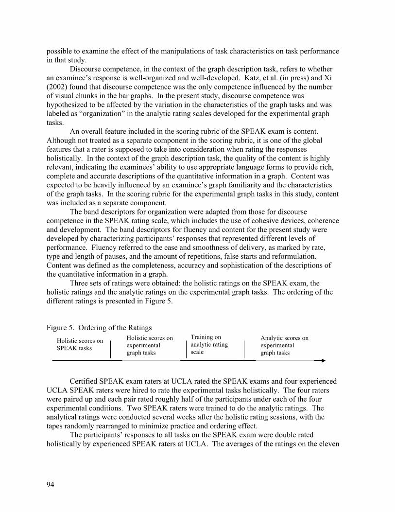
94

possible to examine the effect of the manipulations of task characteristics on task performance in that study.

Discourse competence, in the context of the graph description task, refers to whether an examinee’s response is well-organized and well-developed. Katz, et al. (in press) and Xi (2002) found that discourse competence was the only competence influenced by the number of visual chunks in the bar graphs. In the present study, discourse competence was hypothesized to be affected by the variation in the characteristics of the graph tasks and was labeled as “organization” in the analytic rating scales developed for the experimental graph tasks.

An overall feature included in the scoring rubric of the SPEAK exam is content. Although not treated as a separate component in the scoring rubric, it is one of the global features that a rater is supposed to take into consideration when rating the responses holistically. In the context of the graph description task, the quality of the content is highly relevant, indicating the examinees’ ability to use appropriate language forms to provide rich, complete and accurate descriptions of the quantitative information in a graph. Content was expected to be heavily influenced by an examinee’s graph familiarity and the characteristics of the graph tasks. In the scoring rubric for the experimental graph tasks in this study, content was included as a separate component.

The band descriptors for organization were adapted from those for discourse competence in the SPEAK rating scale, which includes the use of cohesive devices, coherence and development. The band descriptors for fluency and content for the present study were developed by characterizing participants’ responses that represented different levels of performance. Fluency referred to the ease and smoothness of delivery, as marked by rate, type and length of pauses, and the amount of repetitions, false starts and reformulation. Content was defined as the completeness, accuracy and sophistication of the descriptions of the quantitative information in a graph.

Three sets of ratings were obtained: the holistic ratings on the SPEAK exam, the holistic ratings and the analytic ratings on the experimental graph tasks. The ordering of the different ratings is presented in Figure 5. Figure 5. Ordering of the Ratings

Certified SPEAK exam raters at UCLA rated the SPEAK exams and four experienced

UCLA SPEAK raters were hired to rate the experimental tasks holistically. The four raters were paired up and each pair rated roughly half of the participants under each of the four experimental conditions. Two SPEAK raters were trained to do the analytic ratings. The analytical ratings were conducted several weeks after the holistic rating sessions, with the tapes randomly rearranged to minimize practice and ordering effect.

The participants’ responses to all tasks on the SPEAK exam were double rated holistically by experienced SPEAK raters at UCLA. The averages of the ratings on the eleven

Holistic scores on experimental graph tasks

Analytic scores on experimental graph tasks

Training on analytic rating scale

Holistic scores on SPEAK tasks

95

tasks (excluding the SPEAK graph task) on the SPEAK exam were used as indicators of participants’ general speaking proficiency.

For the experimental graph tasks, the raters assigned holistic ratings using the SPEAK Band Descriptors. The raters were asked to indicate whether a score was on the higher end, medium end or lower end of the score band they assigned by checking H, M, or L. The holistic scores, ranging from 20 to 60 in increments of 10, were converted to expanded scores based on where exactly the raters indicated the scores fell on the band, with 3.3 added to a High, 3.3 subtracted from a Low, and a Medium left unadjusted. The converted scores on the graph tasks were used as indicators of the participants’ actual performances.

The participants’ performance was also rated on a 1–5 point scale on fluency, organization, and content. Only whole numbers (1-5) were assigned on the three components. Dependability of Ratings

In order to optimize the design of the rating procedures for the experimental graph tasks and to investigate the dependability of the ratings, univariate and multivariate G studies were conducted using the GENOVA (Crick & Brennan, 1983) and mGENOVA programs (Brennan, 2001) to estimate the magnitude of different sources of variation in the SPEAK exam scores, the holistic ratings, and the analytic ratings on the graph tasks. Both G coefficients and Phi indices were reported.

The results showed that when two raters were used, the G coefficients and Phi indices were both .90 for twelve SPEAK exam tasks and .76 and .75 for one task. The high G coefficients and Phi indices for the combination of twelve tasks and two raters supported the current practice of double rating the SPEAK exam. A decision was thus made to obtain double holistic ratings for the experimental graph tasks to give adequate dependability of scores. Overall, when double ratings were used, the G coefficients and Phi indices for holistic scores on a single experimental graph task were .83 to .87, higher than those for the holistic scores on a single task in the SPEAK exam. Multivariate G studies were conducted on fully-crossed designs of two raters rating a small batch of 36 examinees to look at the dependability of the analytic ratings on the bar and line graph tasks separately and whether the raters could distinguish the three dimensions in the analytic rating scale. The results suggested that using two raters would give reasonably high dependability for the three subscales, the G coefficients for fluency, organization, and content being .83, .60, and .71, and the Phi indices being .81, .60, and .67, respectively. It was decided that double ratings should be obtained for the analytic ratings. An examination of the universe score correlations among the three subscales showed that all of them were highly correlated (see Appendix D). It suggested either that the three dimensions of fluency, organization, and content were closely related or that a rater halo effect was present. Some further training was conducted to make the raters distinguish the three dimensions better. Then the two raters rated the remaining of the tapes, and the dependability of scores on all the analytic ratings (including the first batch of ratings) was estimated. Moderately high dependability could be achieved with double ratings. When two raters were used, the G coefficients for all the analytic ratings on the bar and line graph tasks were .65 to .81 and the phi indices were .63 to .80 (see Appendix E). In summary, the results of the series of univariate and multivariate G studies supported relatively high dependability of scores with double ratings.

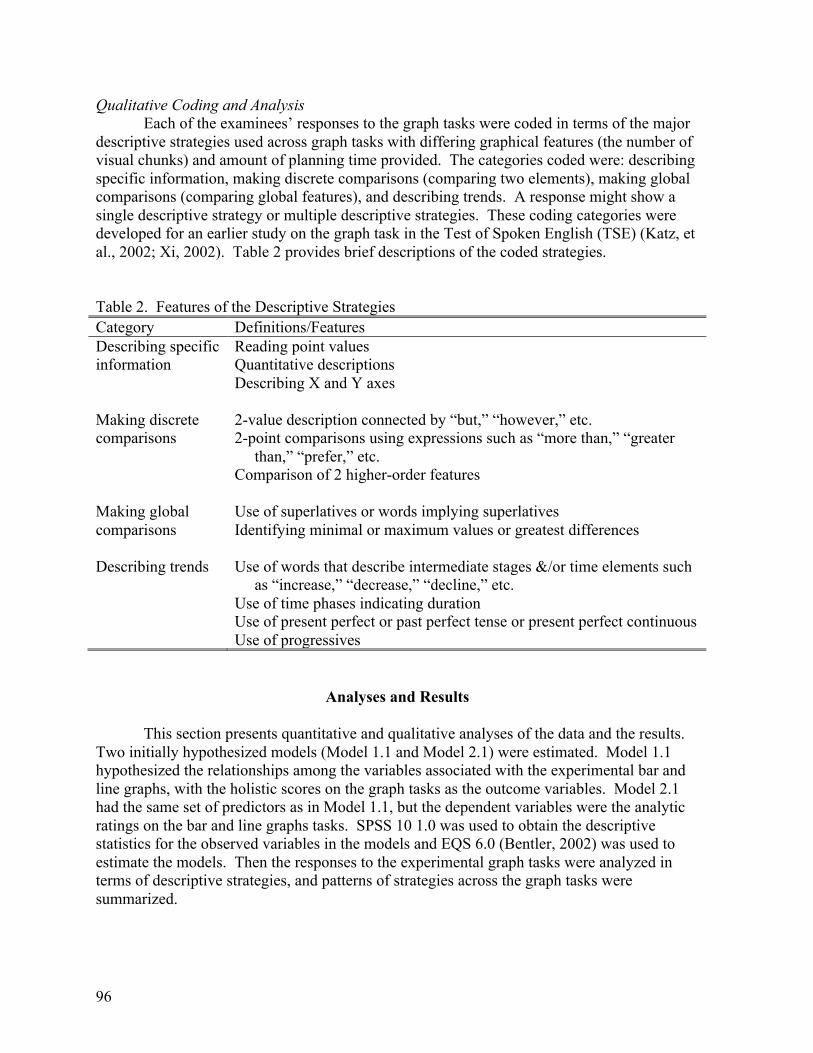
96

Qualitative Coding and Analysis Each of the examinees’ responses to the graph tasks were coded in terms of the major

descriptive strategies used across graph tasks with differing graphical features (the number of visual chunks) and amount of planning time provided. The categories coded were: describing specific information, making discrete comparisons (comparing two elements), making global comparisons (comparing global features), and describing trends. A response might show a single descriptive strategy or multiple descriptive strategies. These coding categories were developed for an earlier study on the graph task in the Test of Spoken English (TSE) (Katz, et al., 2002; Xi, 2002). Table 2 provides brief descriptions of the coded strategies. Table 2. Features of the Descriptive Strategies Category Definitions/Features Describing specific information

Reading point values Quantitative descriptions Describing X and Y axes

Making discrete comparisons

2-value description connected by “but,” “however,” etc. 2-point comparisons using expressions such as “more than,” “greater than,” “prefer,” etc. Comparison of 2 higher-order features

Making global comparisons

Use of superlatives or words implying superlatives Identifying minimal or maximum values or greatest differences

Describing trends Use of words that describe intermediate stages &/or time elements such as “increase,” “decrease,” “decline,” etc. Use of time phases indicating duration Use of present perfect or past perfect tense or present perfect continuous Use of progressives

Analyses and Results

This section presents quantitative and qualitative analyses of the data and the results. Two initially hypothesized models (Model 1.1 and Model 2.1) were estimated. Model 1.1 hypothesized the relationships among the variables associated with the experimental bar and line graphs, with the holistic scores on the graph tasks as the outcome variables. Model 2.1 had the same set of predictors as in Model 1.1, but the dependent variables were the analytic ratings on the bar and line graphs tasks. SPSS 10 1.0 was used to obtain the descriptive statistics for the observed variables in the models and EQS 6.0 (Bentler, 2002) was used to estimate the models. Then the responses to the experimental graph tasks were analyzed in terms of descriptive strategies, and patterns of strategies across the graph tasks were summarized.

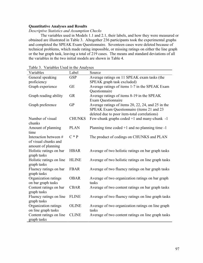
97

Quantitative Analyses and Results Descriptive Statistics and Assumption Checks

The variables used in Models 1.1 and 2.1, their labels, and how they were measured or obtained are illustrated in Table 3. Altogether 236 participants took the experimental graphs and completed the SPEAK Exam Questionnaire. Seventeen cases were deleted because of technical problems, which made rating impossible, or missing ratings on either the line graph or the bar graph task, leaving a total of 219 cases. The means and standard deviations of all the variables in the two initial models are shown in Table 4.

Table 3. Variables Used in the Analyses Variables Label Source General speaking proficiency

GSP Average ratings on 11 SPEAK exam tasks (the SPEAK graph task excluded)

Graph experience GE Average ratings of items 1-7 in the SPEAK Exam Questionnaire

Graph reading ability GR Average ratings of items 8-19 in the SPEAK Exam Questionnaire

Graph preference GP Average ratings of items 20, 22, 24, and 25 in the SPEAK Exam Questionnaire (items 21 and 23 deleted due to poor item-total correlations)

Number of visual chunks

CHUNKS Few-chunk graphs coded +1 and many-chunk -1

Amount of planning time

PLAN Planning time coded +1 and no planning time -1

Interaction between # of visual chunks and amount of planning

C * P The product of codings on CHUNKS and PLAN

Holistic ratings on bar graph tasks

HBAR Average of two holistic ratings on bar graph tasks

Holistic ratings on line graph tasks

HLINE Average of two holistic ratings on line graph tasks

Fluency ratings on bar graph tasks

FBAR Average of two fluency ratings on bar graph tasks

Organization ratings on bar graph tasks

OBAR Average of two organization ratings on bar graph tasks

Content ratings on bar graph tasks

CBAR Average of two content ratings on bar graph tasks

Fluency ratings on line graph tasks

FLINE Average of two fluency ratings on line graph tasks

Organization ratings on line graph tasks

OLINE Average of two organization ratings on line graph tasks

Content ratings on line graph tasks

CLINE Average of two content ratings on line graph tasks

98

Table 4. Descriptive Statistics for the Variables in the Two SEM Models Variable minimum maximum mean SD GSP 31.36 60.00 45.66 5.98 GE 1.00 6.00 4.01 1.11 GR 1.18 6.00 4.40 1.06 GP 2.25 6.00 4.82 0.87 HBAR 30.00 61.65 44.87 5.95 HLINE 31.65 61.65 45.31 5.93 FBAR 1.00 5.00 3.70 0.74 OBAR 2.00 5.00 3.83 0.63 CBAR 2.00 5.00 3.82 0.70 FLINE 1.00 5.00 3.80 0.72 OLINE 2.00 5.00 3.97 0.62 CLINE 2.00 5.00 3.93 0.64

N = 219.

In both models, there were two categorical variables (number of visual chunks and amount of planning time) and their interaction term (the product of them). Although it was intended to have equal numbers of participants in each of the four cells for the bar graph tasks and the line graph tasks, these turned out to be slightly different due to missing data (see Table 5). Table 5. Sample Sizes of Different Cells Graph Chunks Planning N Bar many no planning 56 planning 56 Total 112 few no planning 53 planning 54 Total 107 Total no planning 109 planning 110 Total 219 Line many no planning 56 planning 56 Total 112 few no planning 53 planning 54 Total 107 Total no planning 109 planning 110 Total 219

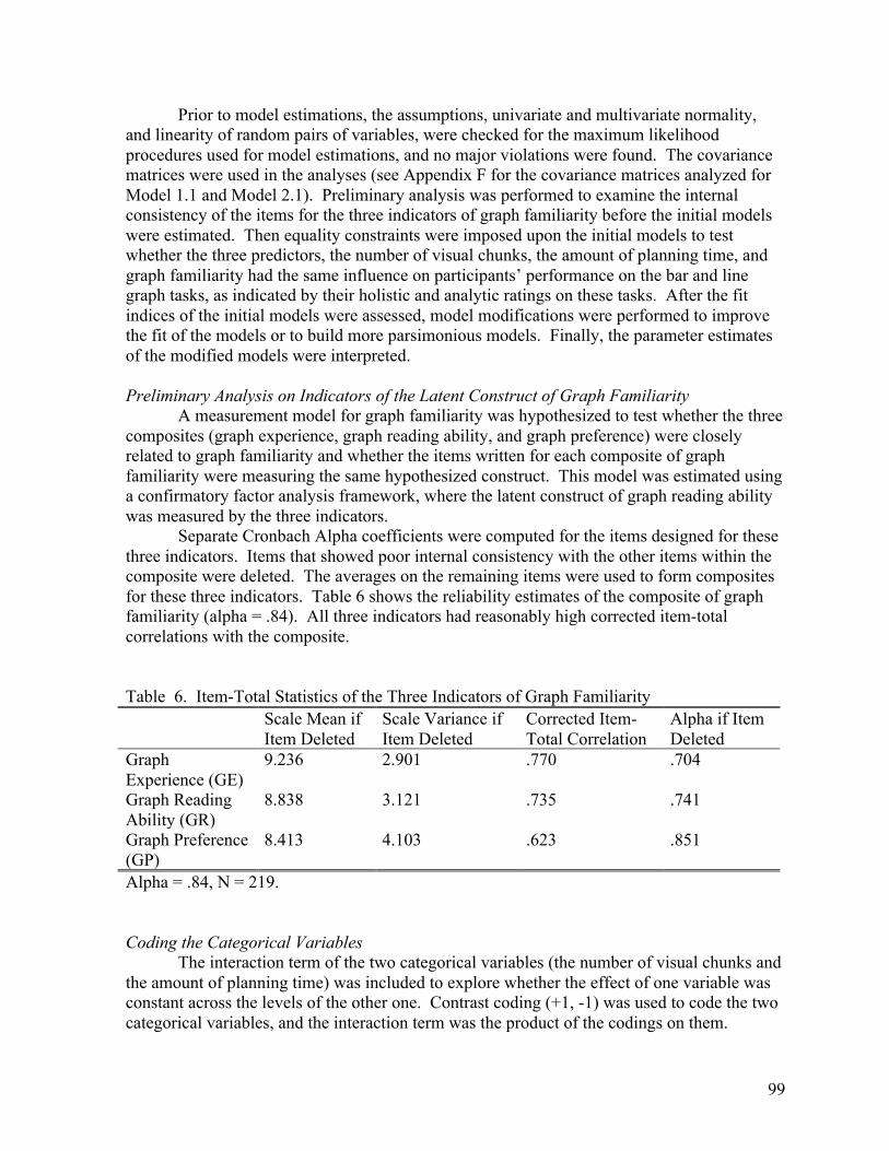
99

Prior to model estimations, the assumptions, univariate and multivariate normality, and linearity of random pairs of variables, were checked for the maximum likelihood procedures used for model estimations, and no major violations were found. The covariance matrices were used in the analyses (see Appendix F for the covariance matrices analyzed for Model 1.1 and Model 2.1). Preliminary analysis was performed to examine the internal consistency of the items for the three indicators of graph familiarity before the initial models were estimated. Then equality constraints were imposed upon the initial models to test whether the three predictors, the number of visual chunks, the amount of planning time, and graph familiarity had the same influence on participants’ performance on the bar and line graph tasks, as indicated by their holistic and analytic ratings on these tasks. After the fit indices of the initial models were assessed, model modifications were performed to improve the fit of the models or to build more parsimonious models. Finally, the parameter estimates of the modified models were interpreted. Preliminary Analysis on Indicators of the Latent Construct of Graph Familiarity

A measurement model for graph familiarity was hypothesized to test whether the three composites (graph experience, graph reading ability, and graph preference) were closely related to graph familiarity and whether the items written for each composite of graph familiarity were measuring the same hypothesized construct. This model was estimated using a confirmatory factor analysis framework, where the latent construct of graph reading ability was measured by the three indicators.

Separate Cronbach Alpha coefficients were computed for the items designed for these three indicators. Items that showed poor internal consistency with the other items within the composite were deleted. The averages on the remaining items were used to form composites for these three indicators. Table 6 shows the reliability estimates of the composite of graph familiarity (alpha = .84). All three indicators had reasonably high corrected item-total correlations with the composite. Table 6. Item-Total Statistics of the Three Indicators of Graph Familiarity Scale Mean if

Item Deleted Scale Variance if Item Deleted

Corrected Item-Total Correlation

Alpha if Item Deleted

Graph Experience (GE)

9.236 2.901 .770 .704

Graph Reading Ability (GR)

8.838 3.121 .735 .741

Graph Preference (GP)

8.413 4.103 .623 .851

Alpha = .84, N = 219. Coding the Categorical Variables

The interaction term of the two categorical variables (the number of visual chunks and the amount of planning time) was included to explore whether the effect of one variable was constant across the levels of the other one. Contrast coding (+1, -1) was used to code the two categorical variables, and the interaction term was the product of the codings on them.

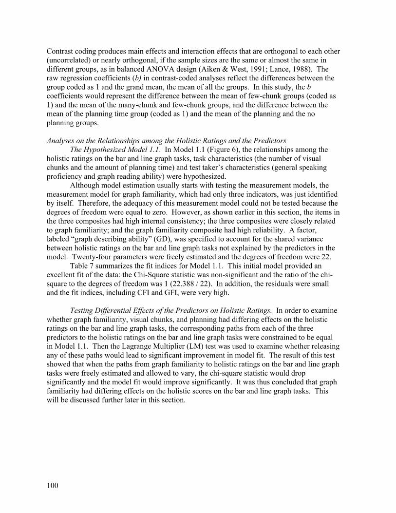
100

Contrast coding produces main effects and interaction effects that are orthogonal to each other (uncorrelated) or nearly orthogonal, if the sample sizes are the same or almost the same in different groups, as in balanced ANOVA design (Aiken & West, 1991; Lance, 1988). The raw regression coefficients (b) in contrast-coded analyses reflect the differences between the group coded as 1 and the grand mean, the mean of all the groups. In this study, the b coefficients would represent the difference between the mean of few-chunk groups (coded as 1) and the mean of the many-chunk and few-chunk groups, and the difference between the mean of the planning time group (coded as 1) and the mean of the planning and the no planning groups. Analyses on the Relationships among the Holistic Ratings and the Predictors

The Hypothesized Model 1.1. In Model 1.1 (Figure 6), the relationships among the holistic ratings on the bar and line graph tasks, task characteristics (the number of visual chunks and the amount of planning time) and test taker’s characteristics (general speaking proficiency and graph reading ability) were hypothesized.

Although model estimation usually starts with testing the measurement models, the measurement model for graph familiarity, which had only three indicators, was just identified by itself. Therefore, the adequacy of this measurement model could not be tested because the degrees of freedom were equal to zero. However, as shown earlier in this section, the items in the three composites had high internal consistency; the three composites were closely related to graph familiarity; and the graph familiarity composite had high reliability. A factor, labeled “graph describing ability” (GD), was specified to account for the shared variance between holistic ratings on the bar and line graph tasks not explained by the predictors in the model. Twenty-four parameters were freely estimated and the degrees of freedom were 22.

Table 7 summarizes the fit indices for Model 1.1. This initial model provided an excellent fit of the data: the Chi-Square statistic was non-significant and the ratio of the chi-square to the degrees of freedom was 1 (22.388 / 22). In addition, the residuals were small and the fit indices, including CFI and GFI, were very high.

Testing Differential Effects of the Predictors on Holistic Ratings. In order to examine

whether graph familiarity, visual chunks, and planning had differing effects on the holistic ratings on the bar and line graph tasks, the corresponding paths from each of the three predictors to the holistic ratings on the bar and line graph tasks were constrained to be equal in Model 1.1. Then the Lagrange Multiplier (LM) test was used to examine whether releasing any of these paths would lead to significant improvement in model fit. The result of this test showed that when the paths from graph familiarity to holistic ratings on the bar and line graph tasks were freely estimated and allowed to vary, the chi-square statistic would drop significantly and the model fit would improve significantly. It was thus concluded that graph familiarity had differing effects on the holistic scores on the bar and line graph tasks. This will be discussed further later in this section.

101

Figure 6. Initially Hypothesized Model with Holistic Ratings as Dependent Variables (Model 1.1) 1 * * * * * E5* *

a* * * a* * E6* * * *

* freely estimated 1--variance or path fixed to 1

HBAR

GF

CHUNKS

PLAN

C * P

GSP

GP

GR

GE

HLINE

GSP: General speaking proficiency GD: Graph describing ability CHUNKS: # of visual chunks GE: Graph experience PLAN: Amount of planning time GR: Graph reading ability C * P: Interaction CHUNKS & PLAN GP: Graph preference HBAR: Holistic scores on bar graph tasks GF: Graph familiarity HLINE: Holistic scores on line graph tasks

1 GD

E7*

E8*

E9*

102

Table 7. Goodness of Fit Summary for Model 1.1 Multivariate Kurtosis Mardia's Coefficient (G2,P) -2.1518 Normalized estimate -1.1315 Residuals Average absolute standardized residuals .0323 Average off-diagonal absolute standardized residuals .0403 Model CHI-SQUARE Goodness of fit summary for method ML Independence model CHI-SQUARE (df = 36) 1004.646 CHI-SQUARE (df = 22) 22.388 Probability value for the CHI-SQUARE statistic .43694 Fit Indices Comparative Fit Index (CFI) 1.000 LISREL GFI Fit Index .977

Final Model 1.2. The result of the LM test was used to see if any paths could be added to yield a better fitting model. None of the paths suggested by the LM test made any sense substantively. Therefore, no additional paths were added.

The result of the Wald test provided useful statistical information in dropping unnecessary parameters. A decision was made based on the results of the Wald test and theoretical rationales to delete the paths from the interaction term (C * P) to holistic scores on the bar graph tasks (HBAR) and from the number of visual chunks (CHUNKS) to holistic scores on the bar graph tasks (HBAR). Model 1.1 was re-estimated with the two paths dropped. The fit indices for Model 1.2 are presented in Table 8. This modified model yielded an equally excellent fit as Model 1.1, but had more degrees of freedom (df = 24 vs. df = 22). It was thus chosen as the final model for its parsimony. Table 8. Summary of Goodness of Fit Indices for Model 1.2 Residuals Average absolute standardized residuals .0316 Average off-diagonal absolute standardized residuals .0394 Model CHI-SQUARE Independence model CHI-SQUARE (df = 36) 1004.646 CHI-SQUARE (df = 24) 25.318 Probability value for the CHI-SQUARE statistic .38865 Fit Indices Comparative Fit Index (CFI) .999 LISREL GFI Fit Index .974

103

Significance of Specific Parameters in Model 1.2 (final model) The final model with significant parameters in both standardized and unstandardized forms is diagrammed in Figure 7. The standardized solutions were interpreted since the unstandardized estimates could not be compared across variables with different scales. However, the unstandardized coefficients of the paths from the number of visual chunks (CHUNKS), the amount of planning time (PLAN) and their interaction term (C * P) to the holistic scores on the bar and line graph tasks (HBAR and HLINE) were interpreted since the original metrics of these variables were meaningful.

Three variables had significant paths to holistic ratings on both bar and line graph tasks: general speaking proficiency (GSP), planning time (PLAN) and graph familiarity (GF). For example, the unstandardized path coefficient from the amount of planning time (PLAN) to the holistic scores on the bar graph tasks (HBAR) was .657. This path coefficient was equal to half of the mean differences in the scores of participants under planning and no planning conditions (Meanplanning – 1 / 2 [Meanplanning + Meannoplanning] = 1 / 2 [Meanplanning – Meannoplanning]). Thus, on average, participants who were presented the bar graph tasks with planning time received about 1.31 (.657 x 2) points higher holistic scores than those under the no planning condition.

Although the interaction term between visual chunks and planning (C * P) was an unimportant predictor of the holistic scores on the bar graph tasks (HBAR) and dropped in the model modification, it turned out to have a significant influence on the holistic scores on the line graph tasks. This indicates that the effect of planning time on the holistic scores was not constant across the many-chunk and the few-chunk line graphs. A follow-up ANCOVA analysis was conducted to examine this interaction effect and will be discussed later in this section. Since this interaction effect was significant, the effect of planning time on the holistic scores on the line graph tasks should be interpreted with caution.

With regard to the influence of graph familiarity, every standard unit increase in graph familiarity self ratings would lead to .161 standard deviation increase in the holistic scores on the bar graph tasks but only .104 standard deviation increase in the scores on the line graph tasks. This result confirmed the differing effects of graph familiarity on the bar and line graph tasks, as shown by the improved model fit when the paths from graph familiarity to the holistic scores on the bar and line graph tasks were allowed to vary. It appears that test takers’ familiarity with statistical graphs had more influence on their performance on the bar graph tasks than on the line graph tasks.

104

Figure 7. Final Model with Holistic Ratings as Dependent Variables (Model 1.2) 1 (. 890) . 901 (.832) . 592 (.675) . 976 (. 161) .626 (.104) (.273) E5 . 805 (. 811)

. 810 2.854 (. 819) (.479) . . 657 2.854 (. 111) (.481) (.276) E6 . 514 (.087) * standardized parameter estimates in parentheses

Analyses on the Relationships among the Analytic Ratings and the Predictors

Hypothesized Model 2.1 (initial model). Model 2.1 hypothesized the relationships among the predictors and the analytic ratings on the bar and line graph tasks. Prior to the estimation of the whole hypothesized Model 2.1, two alternative measurement models for the analytic ratings on the bar and line graph tasks were hypothesized and compared in terms of their model fits and interpretability. The model presented in Figure 8 was chosen because of its superior fit and better interpretability, compared to a model that specified three factors of fluency, organization, and content. The chosen model included three factors, fluency (F), topic development for bar graph tasks (TDB) and topic development for line graph tasks (TDL). Because the development of the topic was defined as part of the descriptors for both

GSP: General speaking proficiency GD: Graph describing ability CHUNKS: # of visual chunks GE: Graph experience PLAN: Amount of planning time GR: Graph reading ability C * P: Interaction CHUNKS & PLAN GP: Graph preference HBAR: Holistic scores on bar graph tasks GF: Graph familiarity HLINE: Holistic scores on line graph tasks

HBAR

GF

CHUNKS

PLAN

C * P

GSP

GP

GR

GE

HLINE

E7 (.456)*

E8 (.555)

E9 (.738)

.360 (.061)

1 GD

105

organization and content, and a high correlation between these two ratings on the same tasks was expected, it was reasonable to specify two topic development factors to explain the covariances between organization and content ratings for the bar and line graph tasks respectively. A higher-order factor, fluency and topic development (FTD), was specified to account for the covariances among these three factors.

The full initially hypothesized model is shown in Figure 9. There were 55 freely estimated parameters and the degrees of freedom were 36. The average off-diagonal standardized residual was very small (.031), showing that the hypothesized model explained the observed covariances among the variables very well. Both the CFI and GFI indices were very high (.987 and .962). The ratio of the chi-square statistic (56.031) to the degrees of freedom (36) was 1.56, which was less than two. All these fit indices provided substantial support for the initial hypothesized model.

Figure 8. The Second Measurement Model for the Analytic Ratings

1 *

* * * 1 * *

* *

1

*

FBAR

OBAR

CBAR

CLINE

OLINE

FLINE TDB

F

TDL LL

1 FTD

CFI=.981 GFI=.962

*

*

*

*

*

*

106

Figure 9. Initially Hypothesized Model with Analytic Ratings as Dependent Variables (Model 2.1) E11*

* estimated parameters 1 1 – variance or path fixed to 1 E12* * * * * * E13* D2* E5* * * * 1 * E6 * *

* D3* * 1 *

* * * * * * E7* * * * * * E8* * * * * * E9* * * D4* * * 1 * * * * E10* *

CHUNKS

PLAN

C * P

GSP

GR

GE

GF

GP

FBAR

OBAR

CBAR

FLINE

OLINE

Cline

TDB

TDL

F

1 FTD

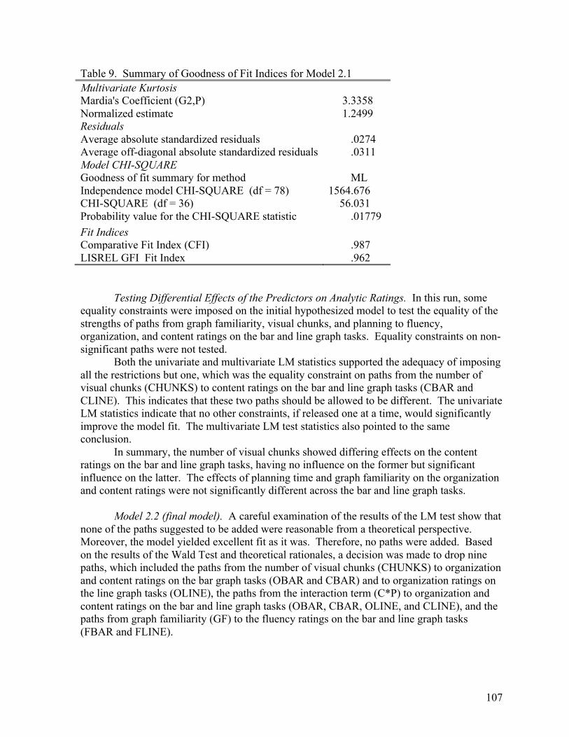
107

Table 9. Summary of Goodness of Fit Indices for Model 2.1 Multivariate Kurtosis Mardia's Coefficient (G2,P) 3.3358 Normalized estimate 1.2499 Residuals Average absolute standardized residuals .0274 Average off-diagonal absolute standardized residuals .0311 Model CHI-SQUARE Goodness of fit summary for method ML Independence model CHI-SQUARE (df = 78) 1564.676 CHI-SQUARE (df = 36) 56.031 Probability value for the CHI-SQUARE statistic .01779 Fit Indices Comparative Fit Index (CFI) .987 LISREL GFI Fit Index .962

Testing Differential Effects of the Predictors on Analytic Ratings. In this run, some equality constraints were imposed on the initial hypothesized model to test the equality of the strengths of paths from graph familiarity, visual chunks, and planning to fluency, organization, and content ratings on the bar and line graph tasks. Equality constraints on non-significant paths were not tested.

Both the univariate and multivariate LM statistics supported the adequacy of imposing all the restrictions but one, which was the equality constraint on paths from the number of visual chunks (CHUNKS) to content ratings on the bar and line graph tasks (CBAR and CLINE). This indicates that these two paths should be allowed to be different. The univariate LM statistics indicate that no other constraints, if released one at a time, would significantly improve the model fit. The multivariate LM test statistics also pointed to the same conclusion. In summary, the number of visual chunks showed differing effects on the content ratings on the bar and line graph tasks, having no influence on the former but significant influence on the latter. The effects of planning time and graph familiarity on the organization and content ratings were not significantly different across the bar and line graph tasks.

Model 2.2 (final model). A careful examination of the results of the LM test show that none of the paths suggested to be added were reasonable from a theoretical perspective. Moreover, the model yielded excellent fit as it was. Therefore, no paths were added. Based on the results of the Wald Test and theoretical rationales, a decision was made to drop nine paths, which included the paths from the number of visual chunks (CHUNKS) to organization and content ratings on the bar graph tasks (OBAR and CBAR) and to organization ratings on the line graph tasks (OLINE), the paths from the interaction term (C*P) to organization and content ratings on the bar and line graph tasks (OBAR, CBAR, OLINE, and CLINE), and the paths from graph familiarity (GF) to the fluency ratings on the bar and line graph tasks (FBAR and FLINE).

108

As can be seen in Table 10, model modifications with the nine paths deleted yielded equally excellent fit indices as in the initially hypothesized model (Model 2.1). The modified model had more degrees of freedom (df = 45) than the initial one (df =36) and was thus selected as the final model for its parsimony. Table 10. Summary of goodness of fit indices for Model 2.2 Residuals Average absolute standardized residuals .0286 Average off-diagonal absolute standardized residuals .0329 Model CHI-SQUARE Independence model CHI-SQUARE (df = 78) 1564.676 CHI-SQUARE (df = 45) 61.633 Probability value for the CHI-SQUARE statistic .38865 Fit Indices Comparative Fit Index (CFI) .989 LISREL GFI Fit Index .959

Significance of Specific Parameters in Model 2.2 (final model). The significant unstandardized parameter estimates and standardized solutions in Model 2.2 are diagrammed in Figure 10.

The first observation was that planning time (PLAN) was a significant predictor of the fluency, organization, and content ratings on both the bar and line graph tasks. Since planning time was contrast-coded, the unstandardized coefficients should be interpreted as half of the difference in the mean scores of the two contrasting experimental conditions. For example, with regard to bar graph tasks, participants under the planning condition scored .35 points (.173 x 2) higher on organization on the bar graph tasks than those who did not receive any planning time. Likewise, the content ratings of students who performed the bar graph tasks with planning time were .30 (.152 x 2) points higher.

The interaction term had a significant influence on the fluency ratings on the bar graph tasks, suggesting that the effects of planning time varied across bar graphs with many and few visual chunks. An ANCOVA analysis was performed to investigate this interaction effect and will be discussed later in this section.

The number of visual chunks (CHUNKS) did not have any influence on the analytic ratings on the bar graph tasks. However, it was a significant predictor of the content ratings of the line graph tasks (CLINE). On average, participants who took the few-chunk line graphs (coded as +1) scored .17 point (.086 x 2) higher on content than students who took the many-chunk graph tasks.

Graph familiarity (GF) was strongly related to the participants’ organization and content ratings on the bar graph tasks, the standardized coefficients being .161 and .178 respectively. However, it did not have a significant influence on their fluency ratings. It appeared that graph familiarity ratings did not have any significant influence on the analytic ratings on the line graph tasks except on content.

109

Figure 10. Final Model with Analytic Ratings as Dependent Variables (Model 2.2)

* standardized solutions in parentheses. E11 (.426)* 1(.904) E12 (.571) . 875 (.821) .101 . 124 .576 (.668) (.161) (.178) E13 (.744) D2 (.612) E5 (.353) . .069 (.108) 1 E6 (.379)

415 (.791) D3 (.714) 1.024 (.750) 1 130 (.176)

173 (.267) .325 (.700) .086 (.135) 1.067 (.712) E7 (.513) .152 (.219) .129 (.180) .163 (.266) .127 (.200) E8 (.328) .377 (.792) .066 (.088) E9 (.324) .072 (.582) D 4 (.611) .048 (.459) 1 .045 (.388) .047 (.463) 065 (.543) .968 (.721) E10 (.488) .044 (.414)

CHUNKS

PLAN

C* P

GSP

GR

GE

GF

GP

FBAR

OBAR

CBAR

FLINE

OLINE

CLINE

TDB

TDL

F

1 FTD

109

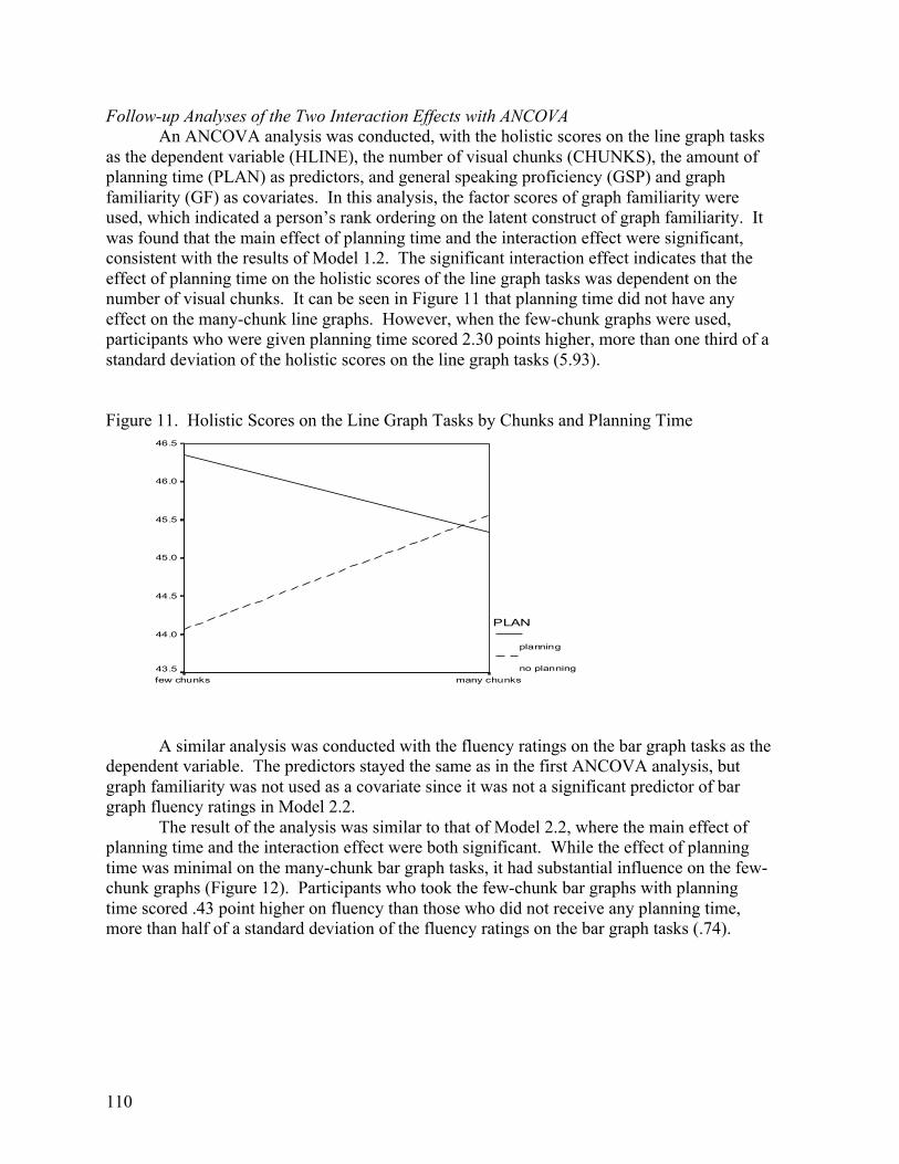
110

Follow-up Analyses of the Two Interaction Effects with ANCOVA An ANCOVA analysis was conducted, with the holistic scores on the line graph tasks

as the dependent variable (HLINE), the number of visual chunks (CHUNKS), the amount of planning time (PLAN) as predictors, and general speaking proficiency (GSP) and graph familiarity (GF) as covariates. In this analysis, the factor scores of graph familiarity were used, which indicated a person’s rank ordering on the latent construct of graph familiarity. It was found that the main effect of planning time and the interaction effect were significant, consistent with the results of Model 1.2. The significant interaction effect indicates that the effect of planning time on the holistic scores of the line graph tasks was dependent on the number of visual chunks. It can be seen in Figure 11 that planning time did not have any effect on the many-chunk line graphs. However, when the few-chunk graphs were used, participants who were given planning time scored 2.30 points higher, more than one third of a standard deviation of the holistic scores on the line graph tasks (5.93).

Figure 11. Holistic Scores on the Line Graph Tasks by Chunks and Planning Time  

A similar analysis was conducted with the fluency ratings on the bar graph tasks as the dependent variable. The predictors stayed the same as in the first ANCOVA analysis, but graph familiarity was not used as a covariate since it was not a significant predictor of bar graph fluency ratings in Model 2.2.

The result of the analysis was similar to that of Model 2.2, where the main effect of planning time and the interaction effect were both significant. While the effect of planning time was minimal on the many-chunk bar graph tasks, it had substantial influence on the few-chunk graphs (Figure 12). Participants who took the few-chunk bar graphs with planning time scored .43 point higher on fluency than those who did not receive any planning time, more than half of a standard deviation of the fluency ratings on the bar graph tasks (.74).

many chunksfew chunks

Estim

ated m

argina

l mea

ns

46.5

46.0

45.5

45.0

44.5

44.0

43.5

PLAN

planning

no planning

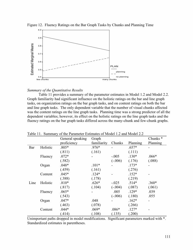
111

Figure 12. Fluency Ratings on the Bar Graph Tasks by Chunks and Planning Time

many chunks few chunks

Es

timate

d Marg

inal M

eans

4.0

3.9

3.8

3.7

3.6

3.5

3.4

PLAN

planning

no planning

Summary of the Quantitative Results Table 11 provides a summary of the parameter estimates in Model 1.2 and Model 2.2. Graph familiarity had significant influence on the holistic ratings on the bar and line graph tasks, on organization ratings on the bar graph tasks, and on content ratings on both the bar and line graph tasks. The only dependent variable that the number of visual chunks affected was the content ratings on the line graph tasks. Planning time was a strong predictor of all the dependent variables; however, its effect on the holistic ratings on the line graph tasks and the fluency ratings on the bar graph tasks differed across the many-chunk and few-chunk graphs. Table 11. Summary of the Parameter Estimates of Model 1.2 and Model 2.2 General speaking

proficiency Graph familiarity

Chunks

Planning

Chunks * Planning

Bar Holistic .805* (.811)

.976* (.161)

- .657* (.111)

-

Fluency .072* (.582)

- -.005 (-.006)

.130* (.176)

.066* (.088)

Organ .048* (.459)

.101* (.161)

- .173* (.276)

-

Content .045* (.388)

.124* (.178)

- .152* (.219)

-

Line Holistic .810* (.817)

.626* (.104)

-.025 (-.004)

.514* (.087)

.360* (.061)

Fluency .065* (.543)

- .005 (-.006)

.129* (.180)

.039

.055 Organ .047*

(.463) .048 (.078)

- .162* (.266)

-

Content .044* (.414)

.069* (.108)

.086* (.135)

.127* (.200)

-

Unimportant paths dropped in model modifications. Significant parameters marked with *. Standardized estimates in parentheses.

112

Results of the Qualitative Analyses This section summarizes the patterns of descriptive strategies that characterize the responses to graph tasks representing each of the four treatment conditions, which were: 1) few-chunk, planning (FCP), 2) few-chunk, no planning (FCNP), 3) many-chunk, planning (MCP), and 4) many-chunk, no planning (MCNP). A single descriptive strategy was used in some of the responses, whereas multiple strategies were used in others. Table 12 shows the percentages of different strategies or combinations of strategies observed in responses to each of the four bar graph tasks. When planning time was not provided, almost the same types of descriptive strategies were used in the responses to the few-chunk and the many-chunk bar graph. Compared to the many-chunk bar graph, slightly larger proportions of responses (58.5% vs. 50.0%) to the few-chunk graph used trend descriptions only or used a combination of trend descriptions and global comparisons (17.0% vs. 10.7%). However, as demonstrated in Figure 13, a greater proportion of the participants who took the many-chunk bar graph without planning time gave two descriptions of two contrasting trends (66.1% vs. 39.6%), namely, the rising enrollment in computers and the declining enrollments in all other courses.

When planning time was provided, similar patterns of descriptive strategies were observed for the many-chunk and the few-chunk bar graphs. Overall, for both graphs, responses that addressed the contrasting trends of computers versus others were predominant. Also, as can be seen in Figure 13 below, a smaller difference in the proportions of responses that discussed the contrasting trends (the differences in the proportions being 13.6% vs. 26.5%) was shown across the many-chunk and the few-chunk graph when planning time was provided. There was also about the same proportion of responses (25.0% vs. 25.9%) that combined trend descriptions and global comparisons (Table 12).

Table 12. Distribution of Descriptive Strategies across the Four Bar Graph Tasks T G DC T + GC T + DC GC + DC D Total FCNP 31 (13) 5 3 (3) 9 (4) 3 (0) 1 (1) 1 53 (21) 58.5% 9.4% 5.7% 17.0% 5.7% 1.9% 1.9% MCNP 28 (20) 6 6 (4) 6 (6) 5 (5) 2 (2) 3 56 (37) 50.0% 10.7% 10.7% 10.7% 8.9% 3.6% 5.4% FCP 28 (25) 6 3 (3) 14 (7) 2 (1) 1 (1) 0 54 (37) 51.9% 11.1% 5.6% 25.9% 3.7% 1.9% 0.0% MCP 27 (24) 4 4 (4) 14 (14) 2 (2) 2 (2) 3 56 (46) 48.2% 7.1% 7.1% 25.0% 3.6% 3.6% 5.4%

FCNP = few-chunk graph, no planning time; MCNP = many-chunk graph, no planning time; FCP = few-chunk graph, planning time; MCP = many-chunk graph, planning time. T = trend descriptions; GC = global comparisons; DC = discrete comparisons; D = descriptions. Numbers in the brackets indicate numbers of responses that addressed the contrasting trends of rising enrollment in computers and declining enrollments in others.

113

Figure 13. Proportion of Responses that Described the Two Contrasting Trends by Bar Graph Tasks

Two separate tables, Tables 13 and 14, were created to illustrate the descriptive

strategies used by participants who took the many-chunk or the few-chunk line graph tasks. As for the many-chunk line graphs, shown in Table 13, mostly trend descriptions were observed; however, the amount of quantitative information covered, defined as the number of line segments described, was different across participants under the planning and no planning conditions.

The majority of the participants who took the many-chunk line graphs with planning time (35 out of 56; 62.5%) described four or five visual chunks (information contained in four or five line segments). In contrast, when no planning time was offered to the participants, more than half of their descriptions of the line graph (29 out of 56; 51.8%) only covered three visual chunks or fewer. Overall, a much greater proportion of descriptions of the many-chunk line graph discussed five chunks when planning time was given than when the graph was processed in an online fashion, as shown in Figure 14. Table 13. Distribution of Descriptive Strategies across the Many-Chunk Line Graph Tasks T GC DC D Total 5C 4C 3C 2C 1C MCNP 11(4) 11 10 13(4) 6 3 1 1 56 (8) 19.6% 19.6% 17.9% 23.2% 10.7% 5.4% 1.8% 1.8% MCP 23(11) 12(7) 11(9) 5(2) 1(1) 0 3 1 56(30) 41.1% 21.4% 19.6% 8.9% 1.8% 0.0% 5.4% 1.8%

T = trend descriptions; 5C = 5 line segments were described (5 visual chunks), GC = global comparisons; DC = discrete comparisons; D = descriptions. Numbers in the brackets indicate the numbers of responses that discussed the overall greater number of tourists to the American city.

0.0% 10.0% 20.0% 30.0% 40.0% 50.0% 60.0% 70.0% 80.0% 90.0%

FCNP MCNP FCP MCP

prop

ortio

ns

bar graph tasks

114

Figure 14. Proportions of Responses Describing Different Amount of Information under Planning and No Planning Conditions

As for the line graph containing two lines, a noticeable difference observed was that a

larger proportion of responses of the participants who did not receive any planning time (15 out of 53; 28.3%) contained trend descriptions not supplemented by global maximum and minimum, discrete comparisons, or point value readings (see Table 14). Table 14. Distribution of Descriptive Strategies across the Few-Chunk Line Graph Tasks T DC T+D T+DC T+GC GC+D T+GC+D T+DC+D Total FCNP 15 0 20 9 4 0 0 5 53 28.3% 0.0% 37.7% 17.0% 7.5% 0.0% 0.0% 9.4% FCP 8 1 25 2 3 1 4 10 54 14.8% 1.9% 46.3% 3.7% 5.6% 1.9% 7.4% 18.5%

FCNP = few-chunk graph, no planning time; FCP = few-chunk graph, planning time; T = trend descriptions; GC = global comparisons; DC = discrete comparisons; D = descriptions.

In summary, some differences were observed in the patterns of descriptive strategies associated with the many-chunk and the few-chunk bar graph tasks, but there was a convergence of patterns when planning time was provided. With regard to the many-chunk line graph tasks, the planning time prompted the participants to process more visual chunks and describe more line segments. For participants who performed the few-chunk line graph task without any planning time, a bigger proportion of their responses contained only trend descriptions not supported by other descriptive strategies.

Discussion

This section presents the findings of this study. The four research questions, the influence of visual chunks and planning on the descriptive strategies, holistic and analytic

0.0% 5.0%

10.0% 15.0% 20.0% 25.0% 30.0% 35.0% 40.0% 45.0%

5C 4C 3C 2C 1C

prop

ortio

n

# of line segments described

MCNP

MCP

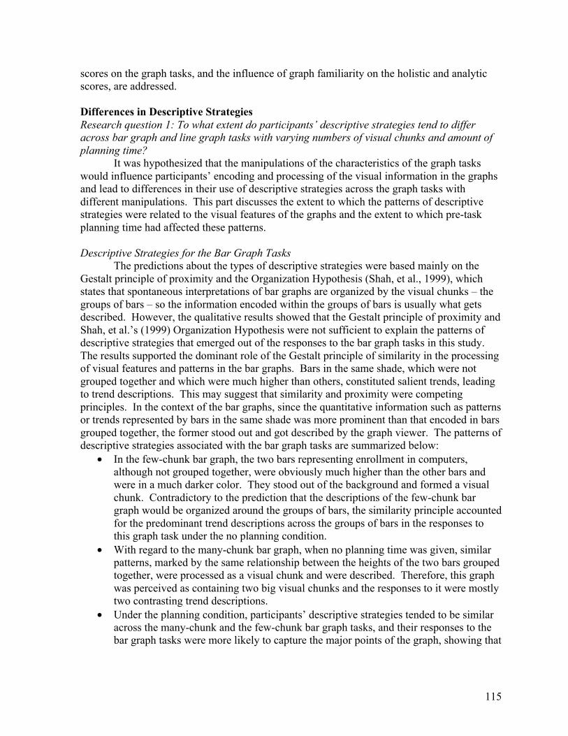
115

scores on the graph tasks, and the influence of graph familiarity on the holistic and analytic scores, are addressed. Differences in Descriptive Strategies Research question 1: To what extent do participants’ descriptive strategies tend to differ across bar graph and line graph tasks with varying numbers of visual chunks and amount of planning time?

It was hypothesized that the manipulations of the characteristics of the graph tasks would influence participants’ encoding and processing of the visual information in the graphs and lead to differences in their use of descriptive strategies across the graph tasks with different manipulations. This part discusses the extent to which the patterns of descriptive strategies were related to the visual features of the graphs and the extent to which pre-task planning time had affected these patterns. Descriptive Strategies for the Bar Graph Tasks

The predictions about the types of descriptive strategies were based mainly on the Gestalt principle of proximity and the Organization Hypothesis (Shah, et al., 1999), which states that spontaneous interpretations of bar graphs are organized by the visual chunks – the groups of bars – so the information encoded within the groups of bars is usually what gets described. However, the qualitative results showed that the Gestalt principle of proximity and Shah, et al.’s (1999) Organization Hypothesis were not sufficient to explain the patterns of descriptive strategies that emerged out of the responses to the bar graph tasks in this study. The results supported the dominant role of the Gestalt principle of similarity in the processing of visual features and patterns in the bar graphs. Bars in the same shade, which were not grouped together and which were much higher than others, constituted salient trends, leading to trend descriptions. This may suggest that similarity and proximity were competing principles. In the context of the bar graphs, since the quantitative information such as patterns or trends represented by bars in the same shade was more prominent than that encoded in bars grouped together, the former stood out and got described by the graph viewer. The patterns of descriptive strategies associated with the bar graph tasks are summarized below:

• In the few-chunk bar graph, the two bars representing enrollment in computers, although not grouped together, were obviously much higher than the other bars and were in a much darker color. They stood out of the background and formed a visual chunk. Contradictory to the prediction that the descriptions of the few-chunk bar graph would be organized around the groups of bars, the similarity principle accounted for the predominant trend descriptions across the groups of bars in the responses to this graph task under the no planning condition.

• With regard to the many-chunk bar graph, when no planning time was given, similar patterns, marked by the same relationship between the heights of the two bars grouped together, were processed as a visual chunk and were described. Therefore, this graph was perceived as containing two big visual chunks and the responses to it were mostly two contrasting trend descriptions.

• Under the planning condition, participants’ descriptive strategies tended to be similar across the many-chunk and the few-chunk bar graph tasks, and their responses to the bar graph tasks were more likely to capture the major points of the graph, showing that

116

planning time could get the participants to engage in more information integration processes.

• Carswell, et al. (1993) suggest that that each trend change represents a visual chunk in a line graph and serves as the unit of description. They also found that changes in the direction of trends formed more readily identifiable visual chunks, whereas change of rate was less noticeable. These findings were confirmed by the results of this study, for both planning and no planning conditions, since almost all the descriptions of the line graph tasks were trend descriptions. However, some differences were observed when the line graph tasks were administered with or without planning time, as discussed in the section of qualitative results.

Influence of Visual Chunks and Planning on Holistic Scores on the Graph Tasks Research question 2: To what extent do examinees’ responses to the graph tasks with different numbers of visual chunks and amounts of planning time tend to get different holistic scores? Is the influence of visual chunks and planning the same across the bar and line graph tasks?

It was found that the participants who took the bar graph tasks with planning time received higher holistic ratings than those who did not have any, which might be a combined effect of planning time on the fluency aspect of linguistic competence, discourse competence and content in the SPEAK holistic rating scale. This seems to imply that the SPEAK raters at UCLA had put more emphasis on aspects in linguistic competence such as pronunciation, grammar, and vocabulary when applying the holistic SPEAK rating scale. Since a participant’s performance on these aspects tends to stay stable across graph tasks that differ in certain dimensions (Katz, et al., in press; Xi, 2002), we would not expect to see big differences in participants’ performances reflected in holistic ratings across the bar graph tasks in this study. As will be discussed later, planning time exerted a much stronger influence on the analytic ratings such as fluency, organization and content.

For the many-chunk line graph, the planning time did not make a difference in the participants’ holistic ratings, whereas for the few-chunk line graph, it improved the participants’ holistic ratings. The many-chunk line graph contained both trend changes and rate changes. As discussed earlier, planning time prompted the participants to describe more line segments and more complex information such as the rate changes associated with the American city. Although they were more ambitious with the content, the accuracy of their language might have been hurt. The potential positive impact of planning on organization and content might have been cancelled out by its negative effect on accuracy.

On the other hand, the few-chunk line graph was processed as two visual chunks under both planning and no planning conditions. Under the planning condition, it elicited a bigger proportion of trend descriptions supported by other descriptive strategies, but this type of description did not necessarily involve using more complex language. Thus, the participants might have benefited by the presence of planning time and presented responses of better organization and content, which were rated higher holistically.

The heavy emphasis on linguistic competence by the raters when using the holistic rating scale might explain why planning time did not have a big effect on the holistic scores, since the only aspect of linguistic competence that might be positively impacted by planning time would be fluency. When fluency was combined with everything else in the holistic rating scale, its influence, if any, was perceived to be smaller.

117

Influence of Visual Chunks and Planning on Analytic Scores on the Graph Tasks Research question 3: To what extent do the number of visual chunks and the amount of planning time influence examinees’ analytic scores on the bar graph and line graph tasks? Is the influence of visual chunks and planning the same across the bar and line graph tasks?

Analytic ratings provided a better picture of how visual chunks and planning would affect the various aspects of one’s language ability, as reflected in the performance on the graph tasks.

With regard to the few-chunk bar graph tasks, the improved fluency under the planning condition suggests that the extra planning time offset the processing load of the few-chunk bar graph and prompted the participants to describe the graphs more smoothly. However, differing effects of planning time on the fluency ratings were seen across the many and few-chunk bar graph tasks since planning time did not have any influence on the fluency ratings on the many-chunk bar graph task. Because the contrasting trends of rising enrollment in computers and declining enrollments in all other courses were not encoded in readily accessible visual chunks in the few-chunk bar graph, the planning time might have helped the participants integrate information and offset the processing load that was demanded of the comprehension of the two contrasting trends. Thus, the participants might have been able to channel more attentional resources to monitor their language and thus might have sounded more fluent.

Although the bar graph with five groups of two bars was designed to be a many-chunk graph (five visual chunks), most participants were drawn to the salient contrasting trend patterns and processed two big visual chunks, driven by the similarity principle. So the effect of planning time might not have played out on this graph that demonstrated prominent contrasting trends.

Participants who were given 60 seconds planning time on the bar graph tasks also scored higher on organization than those who did not receive any planning time. This difference may be because the planning time allowed the participants to study the graph and plan out their responses so that they were more logically connected with appropriate cohesive markers. The analysis of the descriptive strategies demonstrated that when planning time was given, participants’ responses to the bar graph tasks contained more descriptions of the two contrasting trends in enrollments and global comparisons, so they may have been considered as more sophisticated in organization patterns and more developed, thus affecting the organization ratings.

The shifts in patterns of descriptive strategies used for the bar graph tasks under planning and no planning conditions could also explain the gains in participants’ content ratings on the bar graph tasks that gave planning time. When planning time was provided, more participants described the two contrasting trends of enrollments in computers and in other courses. The planning time also helped participants process the global features represented across the five bars in the same shade in the many-chunk bar graph. Overall, the planning time seems to have prompted the participants to present descriptions of the bar graphs that were of stronger content.

The participants who took the line graph tasks with planning time scored on average higher on all the three subscales, fluency, organization and content. When no planning was given, the participants had to process the information in the graphs while describing them and had to create planning time by pausing, repetition, reformulation, etc., so their fluency scores were hurt.

118

There were two reasons for the higher organization ratings on the many-chunk line graph task with planning time. To describe the five trends in this many-chunk line graph in a coherent manner would require quite complex processes involving comparing and contrasting the trends and integrating information. The planning time provided could compensate for the heavy processing load associated with the five visual chunks and allow the participants to organize their descriptions. Second, as was discussed earlier, the descriptions of the many-chunk line graph, when planning time was given, addressed information represented by more line segments and might have been considered more developed responses by the raters. These two factors might explain the more organized responses to the many-chunk line graph task with planning time.

The results of the qualitative analyses indicated that the majority of the responses to the many-chunk line graph when planning time was provided described four or five line segments (four or five visual chunks) and addressed the overall comparison that the American city was visited by more people at all times. The planning time given seems to have allowed the participants to process all the visual chunks and describe them more thoroughly and presented stronger content than those who had to describe it while trying to process the visual information.

With regard to the few-chunk line graph, participants who described it with planning time were more likely to supplement their trend descriptions with other descriptive strategies. Their responses might have been perceived as more developed than just two trend descriptions and were given higher ratings on organization and content.

The only dependent variable that the number of visual chunks had significant influence on was content ratings on the line graph tasks. Higher content ratings on the few-chunk line graph tasks were observed than on the many-chunk line graphs, probably because the many-chunk line graph had five visual chunks to be processed and was more complex than the few-chunk one. The more complex information contained in the many-chunk graph may have made it harder for the participants to describe it completely and accurately.

As for the bar graph tasks, the analytic ratings were not significantly different across the “few-chunk” and the “many-chunk” graphs, because the chunks were not processed as predicted by the proximity principle. Influence of Graph Familiarity Research question 4: To what extent does examinees’ graph reading ability influence their performance on the graph tasks? Is the influence of graph familiarity the same across the bar and line graph tasks?

The result of testing the adequacy of the equality of the paths from graph familiarity to holistic ratings on the bar and line graph tasks supported the conclusion that graph familiarity had a greater impact on participants’ overall holistic performance on the bar graph tasks than on the line graph tasks. The interpretation of bar graphs seemed to involve more complex information processing and integration processes. Visually, the line segments in the line graphs represented linear relationships and were easier to process and describe. This could be shown by the predominant trend descriptions associated with the line graph tasks. On the other hand, any discrete comparisons, global comparisons or trend descriptions of a bar graph would require comparing two or more bars and piecing together several pieces of information. When the overall effectiveness of graph interpretations was broken down into fluency, organization and content, the influence of graph familiarity on specific aspects of the

119

communicative quality could be explored. It was found that graph familiarity had a significant positive influence on the organization and content of the participants’ responses to the bar graph tasks. This suggests that participants with higher graph familiarity were probably more sophisticated in locating, retrieving and integrating information in the bar graphs, and their descriptions were thus stronger in organization and content. One’s graph familiarity, however, did not turn out to be a significant predictor of the fluency ratings on the bar and line graph tasks. This was probably because participants with low graph familiarity could still rely on various strategies to make themselves sound more fluent even when they had trouble processing some information in the graph, especially if they had strong oral skills. With regard to the analytic ratings on the line graph tasks, the only component influenced by one’s graph familiarity was content. Moreover, compared to the bar graph tasks, graph familiarity had a weaker influence on content ratings on the line graph tasks. This indicated that the line graphs in this study were easier to process than the bar graphs. The significant influence of graph familiarity on the overall holistic ratings and some of the analytic ratings posed a serious validity issue. If graph familiarity represented a source of construct-irrelevant variance for the graph description task, this task would be testing not only test takers’ speaking skills, but also their familiarity with graphs. So it would be helpful to use few-chunk graphs and provide planning time so as to mitigate the influence of graph familiarity. Meaningfulness of the Path Coefficients Although the effects of graph familiarity, number of visual chunks, and amount of planning time looked small when translated into raw score differences, these predictors were related to the holistic and analytic scores on the bar and line graph tasks significantly. In addition, the standard deviations of the analytic scores were very small (between .62 and .74), and most of those raw score differences were more than half of a standard deviation of the analytic scores, which supported the strong influences of these predictors on specific components of the participants’ performance. With the whole TSE test-taking population, which is characterized by a wider range of speaking skills and graph familiarity, we might be able to see stronger influences of these predictors as reflected in raw score differences.

Conclusion

This study used an SEM analytic approach to examine the influence of graph task

characteristics and test takers’ graph familiarity on their graph comprehension and interpretation in the context of the SPEAK/TSE exam. It examined differences in oral performance across graph tasks that differed in the way they presented visual chunks of information and across different conditions – with and without planning time. It was found that the participants’ graph familiarity affected the overall communicative quality and some specific components of their performance on these graph tasks. Test takers’ graph familiarity thus represented a potential source of construct-irrelevant variance. However, reducing the number of visual chunks in a graph and providing planning time positively impacted the cognitive processes involved in graph comprehension and helped mitigate the influence of graph familiarity. This could be seen from improved performance under the planning time condition in terms of both holistic and analytic scores and speech samples that showed better

120

comprehension of the information in the graphs, and superior performance on the few-chunk line graph tasks.

This study examined the how guided planning time impacted the quality of oral performance in a controlled setting – the participants were instructed to take one minute to study the graph and think about how they were going to describe the information in the graph. The quality of the discourse produced was compared in terms of fluency, organization, and content. It was found that the participants generally benefited from the planning time and yielded responses that flowed more smoothly, that showed superior organization patterns and more development, and that presented stronger content. From a test validity perspective, providing planning time for the graph description tasks in this study helped reduce the construct irrelevant variance that could have been caused by test takers’ differing degrees of graph familiarity, since under the planning condition, the participants’ responses to the graph tasks captured the major points of the information in the graphs better, and used more sophisticated organization patterns to integrate the information. Planning time in this study did not just function to promote optimal performance; it had the potential to make the graph description task more valid by offsetting the cognitive load involved in graph comprehension and reducing construct-irrelevant variance. Providing planning time for speaking tasks in language tests is usually considered to be at the expense of authenticity, since in real life situations, we are mainly engaged in online planning and processing of utterances and do not usually have preplanning time (Wigglesworth, 1997). However, authenticity is not compromised when planning time is provided for the graph description task, because it is not unusual for one to have some time to plan his/her descriptions of graphs in real life.

Although the manipulation of the number of visual chunks in the bar graphs did not work very well in this study, the results provided insight into the competing roles of proximity and similarity principles in the perception of visual chunks in bar graphs, and the influence of the perceptual organization of the visual information in bar graphs on graph viewers’ verbal interpretations. Practical Implications Designing Graph Tasks in Oral Tests

The results can provide useful guidelines for designing graph tasks in oral assessments. First, planning time should be provided for graph description tasks in oral tests. From a quantitative perspective, with planning time given, the participants can produce responses that are of better overall communicative quality and that are stronger in some individual competencies as well. From a qualitative perspective, planning time can prompt test takers to present more sophisticated descriptions of the quantitative information in the graphs and help elicit more sophisticated organization patterns. Even for graphs that represent the same data but differ in the organization of visual information, planning time allows test takers to use similar descriptive strategies and present similar quantitative information, thus offsetting the processing load associated with a less preferable visual display and mitigating the influence of one’s graph familiarity.

Second, if test takers are given only one minute to study the graph and describe it, we need to make sure that the major points are readily accessible in relatively few visual chunks to minimize the inferential and integration processes that test takers need to go through to understand the major points. If we want to elicit specific language functions such as global

121

comparisons and trend descriptions, we should make the relevant graph features salient in the visual chunks presented to examinees.

It appears that line graphs that have fewer line segments are easier to process and interpret than those that have many line segments. So few-chunk line graphs are recommended to be used. However, if the purpose of the task is to elicit more sophisticated trend descriptions, line graph tasks that have many chunks (preferably representing both trend changes and rates of change) can be used, if sufficient planning time is given.

Although the patterns of descriptive strategies associated with the “few-chunk” and “many-chunk” bar graphs did not support my predictions, they cast some light on the design of bar graphs tasks in speaking tests. If there are quite a few groups of bars, they should be arranged in a way that supports the emergence of salient patterns, as in the “many-chunks” bar graph used in this study. Specifications of the Graph Description Task

In the TSE test specifications, the statement of intended function of the graph description task is very general and vague. The results of the qualitative analysis should help tighten up the specifications for this task. More specific intended language functions, such as making discrete and global comparisons, describing trends and making predictions, should be given as part of the specifications for this task. Also, the question should be revised to maximize the possibility that test takers produce these functions. Rater Training The TSE raters, instead of basing their judgments on personal preferences and experiences, should be given more specific training about what types of responses accomplish the intended language functions of the graph description task and what do not. For example, a response that just describes the axes and contains point value readings should be rated lower than one that uses sophisticated language functions to describe major patterns or trends. This becomes especially relevant when an analytic rating scale is used for the graph description task, where the raters assign componential ratings such as organization and content.

Limitations and Directions for Future Research

Although there is substantial support for the two final hypothesized models in terms of goodness-of-fit indices, cross-validation studies are needed to make sure that the models hold with other samples and that model estimates are stable across samples.

The findings of this study can enrich theories of graph comprehension and interpretation and provide useful guidelines for designing speaking tasks that use graphics as visual prompts; however, the generalizations of the results of this study might be constrained by factors such as the characteristics of the participants, the methodologies used in this study, the rating scales used in this study, and the characteristics of the experimental graph tasks. Therefore, future studies are needed to explore the validity of using other kinds of visual prompts in language assessments with different populations. Also some further research is needed to explore how contextualization can activate test takers’ graph reading schema to search for visual information in the graph to present for a certain purpose and to a specific audience. They may select different information in the graphs to present and choose description strategies different from the ones purely driven by the visual features of the

122

graphs. Moreover, the topical content of the graph might have great impact on the quality of the interpretation, especially for second language speakers. This research question was not investigated in this study but deserves further exploration.

This study analyzed the speech samples to shed light on what visual features in the graphs might have affected the perceptual processes that the participants were engaged in and driven their descriptions. However, we have no way of knowing what the participants exactly attended to during the planning time. Some concurrent and retrospective verbal protocols and interviews might provide some insight into this and buttress results of the analyses on descriptive strategies.

Acknowledgments

I would like to express my sincere thanks to the English Language Institute of the

University of Michigan for funding this research project.

References Aiken, L.S., & West, S. G. (1991). Multiple regression: Testing and interpreting interactions.

Newbury Park, CA: Sage. Bachman, L. F. (1990). Fundamental considerations in language testing. Oxford: Oxford

University Press. Bachman, L. F., & Palmer, A. S. (1996). Language testing in practice. Oxford: Oxford

University Press. Bentler, P. M. (2002). EQS for Windows 6.0. [computer software]. Encino, CA: Multivariate

Software, Inc. Brennan, R. L. (2001). Manual for mGENOVA. Version 2.1. (Occasional Papers No. 50).

Iowa City, IA: Iowa Testing Programs. Butterworth, B. (1980). Some constraints on models of language production. In B.

Butterworth (Ed), Language production. Vol. 1. (pp. 423–459) New York: Academic Press.

Carpenter, P. A., & Shah, P. (1998). A model of the perceptual and conceptual processes in graph comprehension. Journal of Experimental Psychology: Applied, 4(2), 75-100.

Carswell, C. M. (1993). Stimulus complexity and information integration in the spontaneous interpretations of line graphs. Applied Cognitive Psychology, 7(4), 341-357.

Carswell, C. M., Bates, J. R., Pregliasco, N. R., Lonon, A., & Urban, J. (1998). Finding graphs useful: Linking preference to performance for one cognitive tool. Cognitive Technology, 3(1), 4-18.

Carswell, C. M., Emery, C., & Lonon, A. (1993). Stimulus complexity and information integration in the spontaneous interpretation of line graphs. Applied Cognitive Psychology, 7(4), 341-357.

Carswell, C. M., & Ramzy, C. (1997). Graphing small data sets: should we bother? Behavior & Information Technology, 16(2), 61-71.

Crick, J. E. & Brennan, R. L. (1983). Manual for GENOVA: A generalized analysis of variance system. (ACT Technical Bulletin No. 43). Iowa City, IA: ACT, Inc.

Crookes, G. (1989). Planning and interlanguage variation. Studies in Second Language Acquisition, 11(4), 367-383.

123

Educational Testing Service (2001). TSE and SPEAK Band Descriptor Chart. In TSE and SPEAK score user guide: 2001-2002 edition. Princeton, NJ: Educational Testing Service.

Ellis, R. (1987). Interlanguage variability in narrative discourse: Style shifting in the use of the past tense. Studies in Second Language Acquisition, 9(1), 1-20.

Ellis, R. (1994). The study of second language acquisition. Oxford: Oxford University Press. Foster, P., & Skehen, P. (1996). The influence of planning and task type on second langauge

performances. Studies in Second Language Acquisition, 18(3), 299-323. Ginther, A. (2001). Effects of the presence and absence of visuals on performance on TOEFL

CBT listening-comprehensive stimuli. (TOEFL Research Report No. 66). Princeton, NJ: Educational Testing Service.

Gruba, P. (1997). The role of video media in listening assessment. System, 25(3), 335- 346. Gruba, P. (1999). The role of digital media in second language listening comprehension.

Unpublished doctoral thesis, University of Melbourne, Melbourne, Australia. Iwashita, N., McNamara, T., & Elder C. (2001). Can we predict task difficulty in an oral

proficiency test? Exploring the potential of an information-processing approach to task design. Language Learning, 51(3), 401-436.

Katz, I. R., Xi, X., Kim, H., & Cheng, P. C-H. (2002). Graph structure supports graph description. Proceedings of the Twenty-fourth Annual Meeting of the Cognitive Science Society (pp. 157-162). Hillsdale, NJ: Erlbaum.

Katz, I. R., Xi, X., Kim, H., & Cheng, P. C-H. (In press). Elicited speech from graph Items on the Test of Spoken English. (TOEFL Research Report, No. 74). Princeton, NJ: Educational Testing Service.

Kosslyn, S. M. (1989). Understanding charts and graphs. Applied Cognitive Psychology, 3(3),185-225.

Lance, C. E. (1988). Residual centering, exploratory and confirmatory moderator analysis, and decomposition of effects in path models containing interaction effects. Applied Psychological Measurement, 12(2), 163-175.

Mehnert, U. (1998). The effects of different lengths of time for planning on second language performance. Studies in Second Language Acquisition, 20(1), 83-106.

Peebles, D., Cheng, P. C-H., & Shadbolt, N. (2000). Cognitive dimensions of graph-based reasonsing: The role of visual features, knowledge and search. Unpublished manuscript.

Pinker, S. (1990). A theory of graph comprehension. In R. Freedle (Ed.), Artificial intelligence and the future of testing (pp. 73–126). Mahwah, NJ: Erlbaum.

Robinson, P. (1995). Task complexity and second language narrative discourse. Language Learning, 45(1), 141-175.

Robinson, P. (1996). Introduction: Connecting tasks, cognition and syllabus design. The University of Queensland Working Papers in Language and Linguistics, 1, 1-14.

Robinson, P. (2001). Task complexity, task difficulty, and task production: exploring interactions in a componential framework. Applied Linguistics, 22(1), 27-57.

Robinson, P. (2003). Attention and memory during SLA. In C. Doughty and M. Long (Eds.), Handbook of research in second language acquisition (pp.631-678 ). Oxford: Blackwell.

Shah, P. (1995). Cognitive processes in graph comprehension.Unpublished doctoral dissertation, Carnegie Mellon University, Pittsburgh, PA.

124

Shah, P., & Carpenter, P. A. (1995). Conceptual limitations in comprehending line graphs. Journal of Experimental Psychology: General, 124, 43-61.

Shah, P., Hegarty, M., & Mayer, R. E. (1999). Graphs as aids to knowledge construction: Signaling techniques for guiding the process of graph comprehension. Journal of Educational Psychology, 91(4), 690-702.

Skehan, P. (1996). A framework for the implementation of task-based instruction. Applied Linguistics, 17(1), 38-62.

Skehan, P. (1998). A cognitive approach to language learning. Oxford: Oxford University Press.

Wigglesworth, G. (March, 1995). The effect of planning time on oral test discourse. Paper presented at the 17th Language Testing Research Colloquium, Baltimore, MD.

Wigglesworth, G. (1997). An investigation of planning time and proficinecy level on oral test disourse. Language Testing, 14 (1), 85-106.

Wigglesworth, G. (2001). Influences on performance in task-based oral assessments. In M. Bygate, P. Skehan & M. Swain. (Eds.) Researching pedagogical tasks: Second language learning, teaching and testing (pp. 186-209). Harlow: Pearson Education Limited.

Xi, X. (2002). Factors affecting graph comprehension and interpretations by non-native speakers of English. Unpublished manuscript.

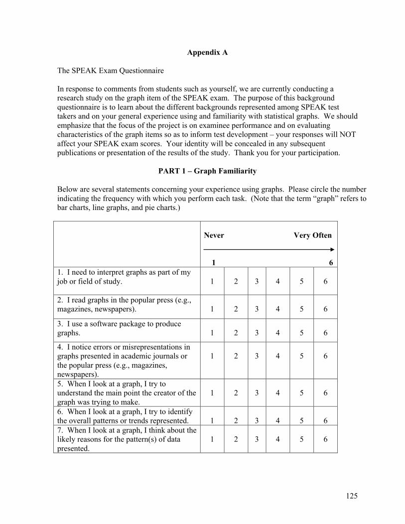
125

Appendix A

The SPEAK Exam Questionnaire

In response to comments from students such as yourself, we are currently conducting a research study on the graph item of the SPEAK exam. The purpose of this background questionnaire is to learn about the different backgrounds represented among SPEAK test takers and on your general experience using and familiarity with statistical graphs. We should emphasize that the focus of the project is on examinee performance and on evaluating characteristics of the graph items so as to inform test development – your responses will NOT affect your SPEAK exam scores. Your identity will be concealed in any subsequent publications or presentation of the results of the study. Thank you for your participation.

PART 1 – Graph Familiarity

Below are several statements concerning your experience using graphs. Please circle the number indicating the frequency with which you perform each task. (Note that the term “graph” refers to bar charts, line graphs, and pie charts.)

Never Very Often

1 6

1. I need to interpret graphs as part of my job or field of study.

1

2

3

4

5

6

2. I read graphs in the popular press (e.g., magazines, newspapers).

1

2

3

4

5

6

3. I use a software package to produce graphs.

1

2

3

4

5

6

4. I notice errors or misrepresentations in graphs presented in academic journals or the popular press (e.g., magazines, newspapers).

1

2

3

4

5

6

5. When I look at a graph, I try to understand the main point the creator of the graph was trying to make.

1

2

3

4

5

6

6. When I look at a graph, I try to identify the overall patterns or trends represented.

1

2

3

4

5

6

7. When I look at a graph, I think about the likely reasons for the pattern(s) of data presented.

1

2

3

4

5

6

126

Below are several questions concerning your graph-reading ability. Please circle the number indicating the extent to which you agree or disagree with each statement.

Strongly Strongly Disagree Agree

1 6

8. I can recognize the components of graphs (e.g., X & Y axes, legend boxes) and how these components combine to represent information.

1

2

3

4

5

6

9. I understand the relationship between a graph and the numerical data it represents.

1 2 3 4 5 6

10. I can identify and interpret complex relationships or patterns displayed in graphs.

1 2 3 4 5 6

11. I can recognize when one graph is a better representation of data than another.

1 2 3 4 5 6

12. I can translate a graph into a verbal description.

1 2 3 4 5 6

13. I can translate a verbal description of a situation (e.g., general trends) to a graph.

1 2 3 4 5 6

14. I can identify a poorly constructed graph. 1 2 3 4 5 6

15. I can revise a poorly constructed graph to improve it.

1 2 3 4 5 6

16. I am familiar with reading line graphs. 1 2 3 4 5 6

17. I am familiar with reading bar graphs. 1 2 3 4 5 6

18. I am familiar with reading pie charts, sometimes called circular charts.

1 2 3 4 5 6

19. Overall, on a scale of 1 to 6, how would you rate your ability to read graphs? 1 2 3 4 5 6 Very weak Very strong

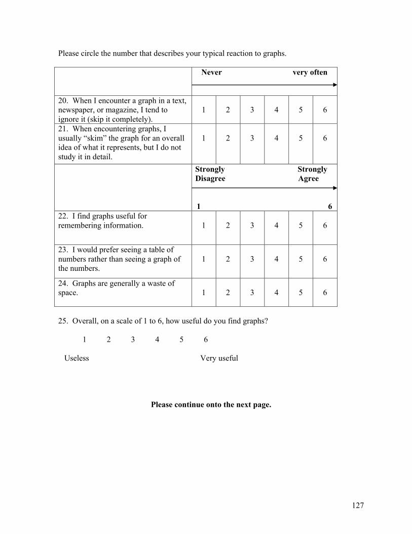
127

Please circle the number that describes your typical reaction to graphs. Never very often

20. When I encounter a graph in a text, newspaper, or magazine, I tend to ignore it (skip it completely).

1

2

3

4

5

6

21. When encountering graphs, I usually “skim” the graph for an overall idea of what it represents, but I do not study it in detail.

1

2

3

4

5

6

Strongly Strongly Disagree Agree

1 6

22. I find graphs useful for remembering information.

1

2

3

4

5

6

23. I would prefer seeing a table of numbers rather than seeing a graph of the numbers.

1

2

3

4

5

6

24. Graphs are generally a waste of space.

1

2

3

4

5

6

25. Overall, on a scale of 1 to 6, how useful do you find graphs? 1 2 3 4 5 6 Useless Very useful

Please continue onto the next page.

128

Part II – General Background 1. UCLA Student ID number _____________ 2. Age _____ 3. Gender _____Female _____Male 4. Native language(s) ________________________________________________ 5. For how many years have you been in the United States?

a. less than one year b. one to five years c. five to ten years d. more than ten years 6. What was/were your undergraduate major(s)? 7. What is/are your graduate degree specialty(ies)? 8. Please fill in your scores on the GRE. If you do not remember your exact score, please write in your best estimate. As with all of the information you provided at this testing session, all your responses will be kept strictly confidential. GRE Math _______ Analytic _________ Approx. date last taken _________ 9. Have you taken any math or statistics classes during your undergraduate and graduate studies? How many have you taken? Math ___ yes ___ no how many _______ Statistics ___ yes ___ no how many _______ 10. How many times have you taken the SPEAK exam (not counting the one you are taking today)? ________________ Please list the test dates and scores: Month/Year Score __________ __________ __________ __________ __________ __________ __________ __________ __________ __________

Thank you very much for your participation!

129

Appendix B The SPEAK Band Descriptors

SPEAK Band Descriptor Chart

Overall features to consider:

60 Communication almost always effective: task performed very competently Speaker volunteers information freely, with little or no effort, and may go beyond the task by using additional appropriate tasks. • Native-like repair strategies

• Sophisticated expressions

• Very strong content • Almost no listener effort required

50 Communication generally effective: task performed competently Speaker volunteers information, sometimes with effort; usually does not run out of time. • Linguistic

weaknesses may necessitate some repair strategies that may be slightly distracting

• Expressions sometimes awkward

• Generally strong content

• Little listener effort required

40 Communication somewhat effective; task performed somewhat competently Speaker responds with effort; sometimes provides limited speech sample and sometimes runs out of time. • Sometimes

excessive, distracting, and ineffective repair strategies used to compensate for linguistic weaknesses (e.g., vocabulary and/or grammar)

• Adequate content • Some listener

effort required

30 Communication generally not effective: task generally performed poorly Speaker responds with much effort; provides limited speech sample and often runs out of time. • Repair strategies

excessive, very distracting, and ineffective

• Much listener effort required

• Difficult to tell if task is fully performed because of linguistic weaknesses, but task can be identified

20 No effective communication; no evidence of ability to perform task Extreme speaker effort is evident; speaker may repeat prompt, give up on task, or be silent. • Attempts to

perform task end in failure

• Only isolated words or phrases intelligible, even with much listener effort

• Task cannot be identified

Function performed clearly and effectively

Task generally performed clearly and effectively

Task performed somewhat clearly and effectively

Task generally performed unclearly and ineffectively

No evidence that task was performed

Functional competence is the speaker’s ability to select functions to reasonably address the task and to select the language needed to carry out the task.

Speaker is highly skillful in selecting language to carry out intended functions that reasonably address the task.

Speaker is able to select language to carry out intended functions that reasonably address the task.

Speaker may lack skills in selecting language to carry out intended functions that reasonably address the task..

Speaker often lacks skill in selecting language to carry out intended functions that reasonably address the task.

Speaker is unable to select language to carry out the function.

Appropriate response to audience/situation

Generally appropriate response to audience/situation

Somewhat appropriate response to audience/situation

Generally inappropriate response to audience/situation

No evidence of ability to respond appropriately to audience/situation

Sociolinguistic competence is the speaker’s ability to demonstrate an awareness of audience and situation by selecting language, register (level of formality), and affective tone, that is appropriate.

Speaker almost always considers register and demonstrates audience awareness.

• Understanding of context, and strength in discourse and linguistic competence, demonstrate sophistication

Speaker generally considers register and demonstrates sense of audience awareness. Occasionally lacks extensive range, variety, and sophistication; response may be slightly unpolished

Speaker demonstrates some audience awareness, but register is not always considered. Lack of linguistic skills that would demonstrate sociolinguistic sophistication

Speaker usually does not demonstrate audience awareness since register is often not considered. Lack of linguistic skills generally masks sociolinguistic skills

Speaker is unable to demonstrate sociolinguistic skills and fails to acknowledge audience or consider register.

130

Coherent, with effective use of cohesive devices

Coherent, with effective use of cohesive devices

Somewhat coherent, with some use of cohesive devices

Generally incoherent, with little use of cohesive devices

Incoherent, with no use of cohesive devices

Discourse competence is the speaker’s ability to develop and organize information in a coherent manner and to make effective use of cohesive devices to help the listener follow the organization of the response.

Response is coherent, with logical organization and clear development. • Contains enough

relevant details to almost always be effective

• Sophisticated cohesive devices result in smooth connection of ideas

Response is generally coherent, with generally clear, logical organization and adequate development.

• Contains enough relevant details to be generally effective

• Some lack of sophistication in use of cohesive devices may detract from smooth connection of ideas

Coherence of the response is sometimes affected by lack of development and/or somewhat illogical or unclear organization, sometimes leaving the listener confused.

• May lack relevant details

• Mostly simple cohesive devices are used

• Somewhat abrupt openings and closures

Response is often incoherent; loosely organized and inadequately developed or disjointed discourse often leave the listener confused.

• Often lacks detail • Simple

conjunctions used as cohesive devices, if at all

• Abrupt openings and closures

Response is incoherent.

• Lack of linguistic competence interferes with the listener’s ability to assess discourse competence

Use of linguistic features almost always effective; communication not affected by minor errors

Use of linguistic features generally effective; communication generally not affected by errors

Use of linguistic features somewhat effective; communication sometimes affected by errors

Use of linguistic features generally poor; communication often impeded by major errors

Use of linguistic features poor; communication ineffective due to major errors

Linguistic competence is the effective selection of vocabulary, control of grammatical structures, and accurate pronunciation along with smooth delivery in order to produce intelligible speech.

• Errors not noticeable

• Accent not distracting

• Range in grammatical structures and vocabulary

• Delivery often has native-like smoothness

• Errors not unusual, but rarely major

• Accent may be slightly distracting

• Some range in vocabulary and grammatical structures, which may be slightly awkward or inaccurate

• Delivery generally smooth, with some hesitancy and pauses

• Minor and major errors present

• Accent usually distracting

• Simple structures sometimes accurate, but errors in more complex structures common

• Limited ranges in vocabulary; some inaccurate word choices

• Delivery often slow or choppy; hesitancy and pauses common

• Limited linguistic control; major errors present

• Accent very distracting

• Speech contains numerous sentence fragments and errors in simple structures

• Frequent inaccurate word choices; general lack of vocabulary for task completion

• Delivery almost always plodding, choppy, and repetitive; hesitancy and pauses very common

• Lack of linguistic control

• Accent so distracting that few words are intelligible

• Speech contains mostly sentence fragments, repetition of vocabulary, and simple phrases

• Delivery so plodding that only few words are produced

Educational Testing Service (2001).

131

Appendix C

Analytic Rating Scales for the Experimental Graph Tasks

5 very strong

4 strong

3 adequate

2 weak

1 very weak

Fluency refers to the ease and smoothness of delivery, as marked by rate, type and length of pauses, the amount of repetitions, false starts and reformulation

Ø Delivery smooth, effortless, and unhesitating

Ø Delivery generally smooth, with some hesitancy when searching for patterns and expressions Ø There are few noticeably long pauses

Ø Delivery sometimes slow or choppy Ø Some hesitancy, and pauses Ø Some false starts, repetitions and reformulation

Ø Delivery often slow or choppy Ø Hesitancy and pauses common Ø False starts, repetitions and reformulation common

Ø Delivery almost always labored, plodding, choppy, and repetitive Ø Hesitancy, and pauses very common Ø False starts, reformulation very common

Organization is the speaker’s ability to develop and organize information in a coherent manner and to make effective use of cohesive devices to help the listener follow the organization of the response

Description is coherent, with logical organization and clear development Ø Contains enough details to almost always be effective ØSophisticated cohesive devices and a variety of organization patterns result in smooth connection of ideas Ø Major points highlighted

Response is generally coherent, with generally clear, logical organization and adequate development Ø Contains enough details to be generally effective Ø Some lack of sophistication in use of cohesive devices may distract from smooth connection of ideas

Coherence of the response occasionally affected by lack of development and/or somewhat illogical or unclear organization, occasionally leaving the listener confused Ø May lack details occasionally Ø Mostly simple cohesive devices are used

Coherence of the response sometimes affected by lack of development and/or somewhat illogical or unclear organization, sometimes leaving the listener confused Ø May lack details Ø Mostly simple cohesive devices are used and some don’t mark the relationships appropriately Ø Somewhat abrupt openings and closures

Response often incoherent; loosely organized and inadequately developed; disjointed discourse often leaves the listener confused Ø Often lacks details Ø Simple conjunction used as cohesive devices, if at all Ø Abrupt openings and closures

Content refers to the completeness, accuracy, and sophistication in the descriptions of the quantitative information in a graph

Very strong content Ø Rich, complete and accurate descriptions of the quantitative information in a graph Ø Overall trends, patterns, comparisons or predictions thoroughly discussed

Generally strong content Ø Accurate descriptions of the quantitative information in a graph Ø Most of the overall trends, patterns, comparisons or predictions discussed

Adequate content Ø Generally accurate descriptions of the quantitative information in a graph Ø Some overall trends, patterns, comparisons or predictions discussed

Weak Ø Content sometimes weak Ø Sometimes descriptions of the quantitative information not accurate Ø Mostly trivial local comparisons or discrete point value reading Ø Almost no overall trends, patterns, comparisons or predictions discussed

Very weak Ø Content is generally weak Ø One or two point value readings

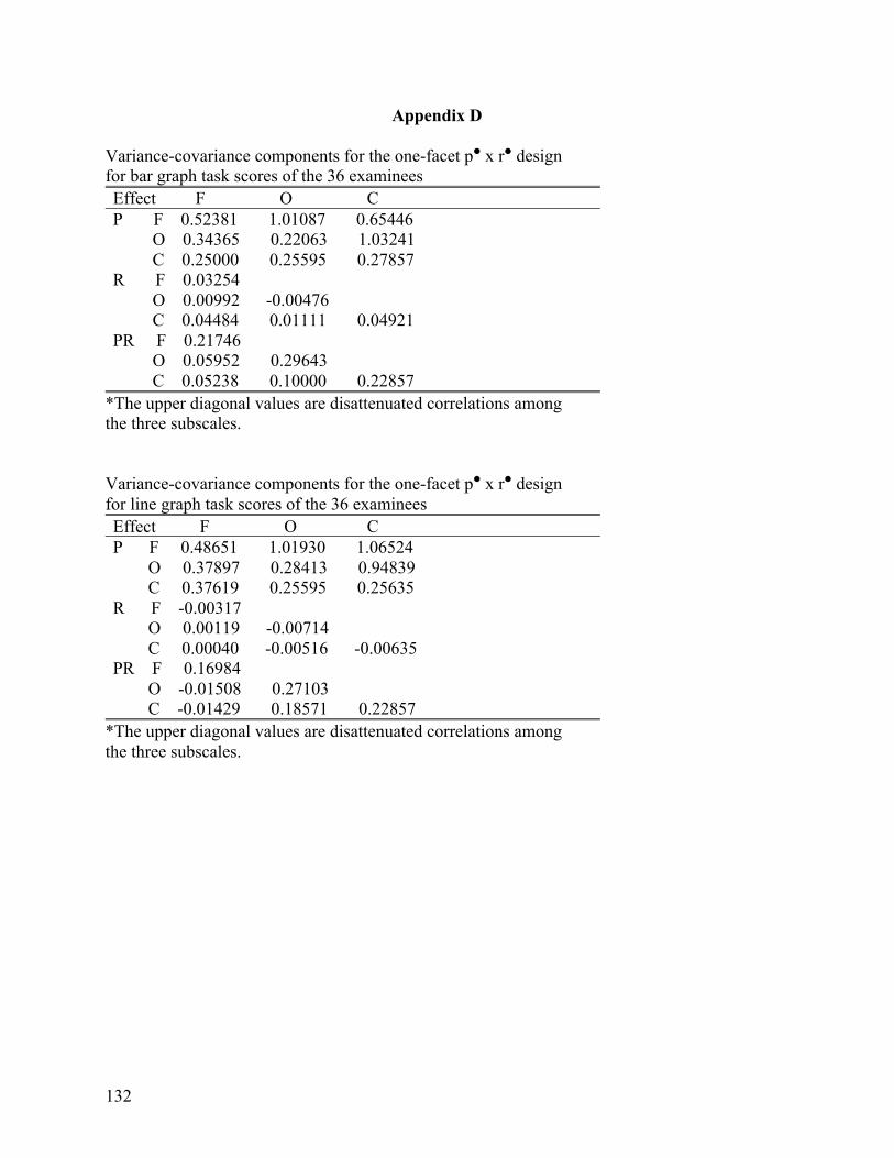
132

Appendix D Variance-covariance components for the one-facet pl x rl design for bar graph task scores of the 36 examinees Effect F O C P F 0.52381 1.01087 0.65446 O 0.34365 0.22063 1.03241 C 0.25000 0.25595 0.27857 R F 0.03254 O 0.00992 -0.00476 C 0.04484 0.01111 0.04921 PR F 0.21746 O 0.05952 0.29643 C 0.05238 0.10000 0.22857

*The upper diagonal values are disattenuated correlations among the three subscales. Variance-covariance components for the one-facet pl x rl design for line graph task scores of the 36 examinees Effect F O C P F 0.48651 1.01930 1.06524 O 0.37897 0.28413 0.94839 C 0.37619 0.25595 0.25635 R F -0.00317 O 0.00119 -0.00714 C 0.00040 -0.00516 -0.00635 PR F 0.16984 O -0.01508 0.27103 C -0.01429 0.18571 0.22857

*The upper diagonal values are disattenuated correlations among the three subscales.

133

Appendix E Results of D studies for the one-facet pl x rl design for bar graph task scores of the 219 examinees nr = 1 nr = 2 F O C F O C Univ Score Var .351 .235 .366 .351 .235 .366 Rel Error Var .162 .256 .223 .081 .128 .112 Abs Error Var .180 .273 .254 .090 .137 .127 Gen Coefficient 0.68 0.48 0.62 0.81 0.65 0.77 Phi 0.66 0.46 0.59 0.80 0.63 0.74 Composite

Gen Coefficient 0.71 0.83 Composite Phi 0.67 0.80

Results of D studies for the one-facet pl x rl design for line graph task scores of the 219 examinees nr = 1 nr = 2 F O C F O C Univ Score Var .303 .237 .286 .303 .237 .286 Rel Error Var .189 .242 .219 .090 .121 .110 Abs Error Var .193 .251 .238 .097 .126 .119 Gen Coefficient 0.61 0.50 0.57 0.76 0.66 0.72 Phi 0.61 0.49 0.55 0.76 0.65 0.71 Composite

Gen Coefficient 0.70 0.82 Composite Phi 0.68 0.81

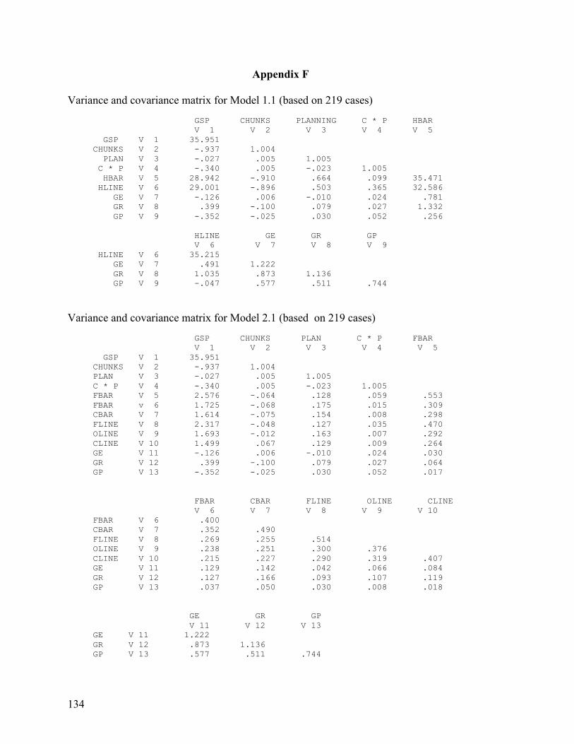
134

Appendix F Variance and covariance matrix for Model 1.1 (based on 219 cases) GSP CHUNKS PLANNING C * P HBAR V 1 V 2 V 3 V 4 V 5 GSP V 1 35.951 CHUNKS V 2 -.937 1.004 PLAN V 3 -.027 .005 1.005 C * P V 4 -.340 .005 -.023 1.005 HBAR V 5 28.942 -.910 .664 .099 35.471 HLINE V 6 29.001 -.896 .503 .365 32.586 GE V 7 -.126 .006 -.010 .024 .781 GR V 8 .399 -.100 .079 .027 1.332 GP V 9 -.352 -.025 .030 .052 .256 HLINE GE GR GP V 6 V 7 V 8 V 9 HLINE V 6 35.215 GE V 7 .491 1.222 GR V 8 1.035 .873 1.136 GP V 9 -.047 .577 .511 .744

Variance and covariance matrix for Model 2.1 (based on 219 cases) GSP CHUNKS PLAN C * P FBAR V 1 V 2 V 3 V 4 V 5 GSP V 1 35.951 CHUNKS V 2 -.937 1.004 PLAN V 3 -.027 .005 1.005 C * P V 4 -.340 .005 -.023 1.005 FBAR V 5 2.576 -.064 .128 .059 .553 FBAR v 6 1.725 -.068 .175 .015 .309 CBAR V 7 1.614 -.075 .154 .008 .298 FLINE V 8 2.317 -.048 .127 .035 .470 OLINE V 9 1.693 -.012 .163 .007 .292 CLINE V 10 1.499 .067 .129 .009 .264 GE V 11 -.126 .006 -.010 .024 .030 GR V 12 .399 -.100 .079 .027 .064 GP V 13 -.352 -.025 .030 .052 .017 FBAR CBAR FLINE OLINE CLINE V 6 V 7 V 8 V 9 V 10 FBAR V 6 .400 CBAR V 7 .352 .490 FLINE V 8 .269 .255 .514 OLINE V 9 .238 .251 .300 .376 CLINE V 10 .215 .227 .290 .319 .407 GE V 11 .129 .142 .042 .066 .084 GR V 12 .127 .166 .093 .107 .119 GP V 13 .037 .050 .030 .008 .018 GE GR GP V 11 V 12 V 13 GE V 11 1.222 GR V 12 .873 1.136 GP V 13 .577 .511 .744

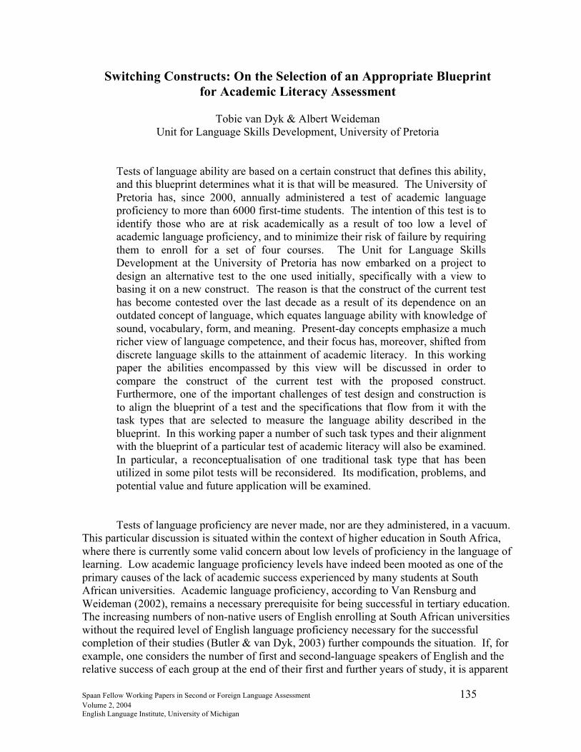
Spaan Fellow Working Papers in Second or Foreign Language Assessment 135 Volume 2, 2004 English Language Institute, University of Michigan

Switching Constructs: On the Selection of an Appropriate Blueprint for Academic Literacy Assessment

Tobie van Dyk & Albert Weideman

Unit for Language Skills Development, University of Pretoria

Tests of language ability are based on a certain construct that defines this ability, and this blueprint determines what it is that will be measured. The University of Pretoria has, since 2000, annually administered a test of academic language proficiency to more than 6000 first-time students. The intention of this test is to identify those who are at risk academically as a result of too low a level of academic language proficiency, and to minimize their risk of failure by requiring them to enroll for a set of four courses. The Unit for Language Skills Development at the University of Pretoria has now embarked on a project to design an alternative test to the one used initially, specifically with a view to basing it on a new construct. The reason is that the construct of the current test has become contested over the last decade as a result of its dependence on an outdated concept of language, which equates language ability with knowledge of sound, vocabulary, form, and meaning. Present-day concepts emphasize a much richer view of language competence, and their focus has, moreover, shifted from discrete language skills to the attainment of academic literacy. In this working paper the abilities encompassed by this view will be discussed in order to compare the construct of the current test with the proposed construct. Furthermore, one of the important challenges of test design and construction is to align the blueprint of a test and the specifications that flow from it with the task types that are selected to measure the language ability described in the blueprint. In this working paper a number of such task types and their alignment with the blueprint of a particular test of academic literacy will also be examined. In particular, a reconceptualisation of one traditional task type that has been utilized in some pilot tests will be reconsidered. Its modification, problems, and potential value and future application will be examined.

Tests of language proficiency are never made, nor are they administered, in a vacuum. This particular discussion is situated within the context of higher education in South Africa, where there is currently some valid concern about low levels of proficiency in the language of learning. Low academic language proficiency levels have indeed been mooted as one of the primary causes of the lack of academic success experienced by many students at South African universities. Academic language proficiency, according to Van Rensburg and Weideman (2002), remains a necessary prerequisite for being successful in tertiary education. The increasing numbers of non-native users of English enrolling at South African universities without the required level of English language proficiency necessary for the successful completion of their studies (Butler & van Dyk, 2003) further compounds the situation. If, for example, one considers the number of first and second-language speakers of English and the relative success of each group at the end of their first and further years of study, it is apparent

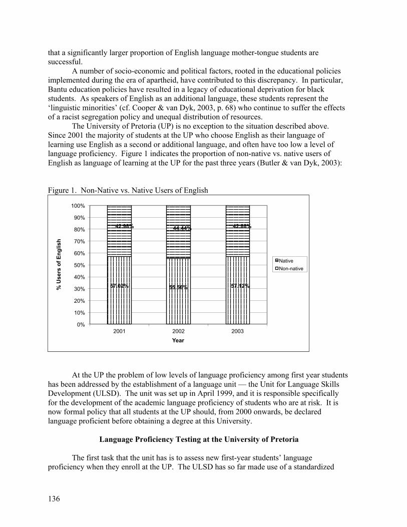
136

that a significantly larger proportion of English language mother-tongue students are successful.

A number of socio-economic and political factors, rooted in the educational policies implemented during the era of apartheid, have contributed to this discrepancy. In particular, Bantu education policies have resulted in a legacy of educational deprivation for black students. As speakers of English as an additional language, these students represent the ‘linguistic minorities’ (cf. Cooper & van Dyk, 2003, p. 68) who continue to suffer the effects of a racist segregation policy and unequal distribution of resources.

The University of Pretoria (UP) is no exception to the situation described above. Since 2001 the majority of students at the UP who choose English as their language of learning use English as a second or additional language, and often have too low a level of language proficiency. Figure 1 indicates the proportion of non-native vs. native users of English as language of learning at the UP for the past three years (Butler & van Dyk, 2003): Figure 1. Non-Native vs. Native Users of English

At the UP the problem of low levels of language proficiency among first year students has been addressed by the establishment of a language unit — the Unit for Language Skills Development (ULSD). The unit was set up in April 1999, and it is responsible specifically for the development of the academic language proficiency of students who are at risk. It is now formal policy that all students at the UP should, from 2000 onwards, be declared language proficient before obtaining a degree at this University.

Language Proficiency Testing at the University of Pretoria

The first task that the unit has is to assess new first-year students’ language

proficiency when they enroll at the UP. The ULSD has so far made use of a standardized

57.02% 55.56% 57.12%

42.98% 44.44% 42.88%

0%

10%

20%

30%

40%

50%

60%

70%

80%

90%

100%

2001 2002 2003

% U

sers

of E

nglis

h

Year

Native Non-native

137

measuring instrument, the English Literacy Skills Assessment for Tertiary Education (ELSA PLUS), that was developed jointly by the University of Pretoria and Hough and Horne Literacy Consultants, in order to determine specific levels of language proficiency. These levels are then used to ascertain whether students need language support in the form of an additional academic language development course (Butler & van Dyk, 2003; Weideman, 2003a).

The purpose of this paper is to report on a study concerning the testing of language proficiency at the University of Pretoria. It will deal first with the construct and features of the ELSA PLUS instrument, as well as the test scores for the years 2001 to 2003. Difficulties with the current construct are then highlighted and, after a consideration of the principles that support the choice of an alternative blueprint, the proposed new construct and its implications will be outlined. The next challenge addressed in this working paper is to find, from the specifications implied in this blueprint, appropriate task types that reliably measure the academic literacy of students in the test population of the UP. Test Subjects

It is compulsory for the approximately 6000 first-year students of the University of Pretoria to sit the ELSA PLUS at the beginning of every year. The test is taken during the academic information week (the week before lectures start) and the results are generally announced no later than the following week. These students form the population on which much of this study was based. Description and Construct of the ELSA PLUS

The ELSA PLUS test was designed and developed in South Africa by the Hough and Horne consultancy on the basis of their industrial and commercial test, the ELSA (English Literacy Skills Assessment) instrument. It was then refined for use at a tertiary institution in collaboration with the ULSD. In keeping with its origins, the test is designed to quantify the competency input levels and trainability of students who need to function effectively in an English language environment. The ELSA PLUS is a norm referenced placement test, where the first language user of English is used as the norm. It is a proficiency test; it is skills-based and not syllabus-based.

The ELSA PLUS consists of seven sections: • Phonics (the ability to recognize and discriminate between English sounds); • Dictation (the ability to write down spoken English and adhere to academic writing

conventions); • Basic numeracy (language use is integrated with an elementary familiarity with numbers); • Reading comprehension (at elementary and intermediate levels); • The language and grammar of spatial relations; • A cloze procedure (the ability to create a semantic whole by completing sentences

coherently); and • Vocabulary in context (the ability to extract the relevant information from a given context

to determine the meaning of certain words or phrases on a basic, academic and advanced level).

It is clear from this description that the test assumes that language ability can best be

defined in terms of its structural components: language is, in this view, a combination of

138

sound, form, and meaning. Also, it is assumed that language use can be captured in terms of a number of ‘skills’, in this case: listening, reading and writing. We return to a consideration of this below.

Some of the salient logistical and administrative features of the ELSA PLUS instrument are that:

• It is a one-hour written assessment. • The scoring is done objectively. • A diagnostic report is available for every participant after completion. • It measures both language skills and language knowledge. • It is culturally fair in that it avoids meta-language, colloquialisms, idiomatic

expressions and dialectic usage. • The test has empirical validity. • Its reliability has been calculated as high as 0.86.

Because the test is norm referenced, it is possible to quantify the language proficiency

of a student in terms of school grades, i.e., formal years of schooling. All first year students who display an inadequate level of language proficiency (Grade 10 level or below, i.e., 10 years of formal schooling) as determined by the ELSA PLUS testing instrument, are required to enroll for a compulsory, fully credit bearing language proficiency course offered by the ULSD. Performance at a Grade 11 level or above currently indicates that no additional language support needs to be undertaken. This, however, does not mean that a student’s language proficiency is perfect or that the level of language ability does not pose a risk of academic underperformance for a student. Therefore, students not required to take the ULSD courses generally choose other language modules offered by the School for Languages that are of the same credit value (12 credits) as the compulsory language proficiency course. This arrangement, however, differs from faculty to faculty, since certain faculties acknowledge different modules for credits. Test Data

Since the year 2000, the percentage of students with language proficiency at a Grade 10 level and lower has stayed consistent at between 27% and 33% as summarized in Table 1.

Table 1. Summary of Test Results since 2000 2000 2001 2002 2003 N = 4661 N = 5215 N = 5788 N = 6472 ≥ Gr.11 ≤ Gr.10 ≥ Gr.11 ≤ Gr.10 ≥ Gr.11 ≤ Gr.10 ≥ Gr.11 ≤ Gr.10 N = 3356 (72%)

N = 1305 (28%)

N = 3495 (67%)

N = 1720 (33%)

N = 4212 (73%)

N = 1576 (27%)

N = 4615 (71%)

N = 1857 (29%)

Problem Statement

There are a number of reasons why a switch from the construct of the ELSA PLUS test is appropriate. The first reason is a practical one, and lies in the logistical constraints that

139

the current instrument has: those who administer the test have to arm themselves with fairly sophisticated sound equipment, stop watches and the like, and should be prepared for a marking period that would, for this number of students, rarely be concluded in under 5 days.

The second reason is that the construct of the current test has become contested over the last decade, as a result of its dependence on an outdated concept of language, which equates language ability with knowledge of sound, vocabulary, form, and meaning. Bachman and Palmer (1996, p. 61ff.) have argued persuasively that tests should, instead, be based on an interactional perspective of language ability, which emphasizes the negotiation of meaning within specific contexts. Similarly, Blanton (1994), even in emphasizing the nature of academic discourse as one in which written language is valued as currency, notes that academically literate behavior involves interacting with texts:

Whatever else we do with L2 students to prepare them for the academic mainstream, we must foster the behaviors of ‘talking’ to texts, talking and writing about them, linking them to other texts, connecting them to their readers’ own lives and experience, and then using their experience to illuminate the text and the text to illuminate their experience. (p. 228)

To see why the view of language held by the test designer is so critical, it is necessary

to take one step back, and consider that a test is always produced for a specific purpose, and that its results inevitably influence decisions about the future of the candidates that take it. Thus, the test developers must always “be able to demonstrate how performance on that language test is related to language use in specific settings” (Bachman & Palmer, 1996, p. 61). Since language performance is interpreted as the outcome of language ability – the exact characteristic of the individual that is being tested – it follows that the definition of language ability is critical for test construction.

Definitions of language ability usually bring together two dimensions of our experience: the lingual and the formative. It is therefore not only language that is being defined, but the extent of the control that the individual has over language. The latter, formative dimension of language use is generally expressed in terms such as ability, competence, mastery and control (cf. Gee, 1998, p. 56-57), capacity, proficiency, authority, power (Blanton, 1994, p. 230), and so forth (for a review, cf. Weideman, 1981, p. 195-204). Definitions of language ability depend, in turn, on the view of language held by the test designer.

For more than thirty years now, it has been accepted that the design of a language test depends on a broader, richer perspective on language than the views held earlier. This is a perspective that goes beyond a restrictive view of language that limits it to a combination of sound, form and meaning, or, in technical linguistic terms, phonological, morphological, syntactic and semantic elements. In line with socially enriched views of language, such a broader framework for language maintains that language is not only expressive, but communicative, intended to mediate and negotiate human interaction. One may summarize the differences between a restrictive and an open view of language, and its implications for learning and testing as shown in the following Table (from Weideman, in press).

140

Table 2. Two Perspectives on Language Restrictive Open Language is composed of elements:

• sound • form, grammar • meaning

Language is a social instrument to: • mediate and • negotiate human interaction • in specific contexts

Main function: expression Main function: communication Language learning = mastery of structure Language learning = becoming competent

in communication Focus: language Focus: process of using language

The table includes, under the rubric of ‘Focus,’ a point that is important not only for teaching and learning, but also for testing. As Blanton (1994, p. 231) points out, language classes that foster academic literacy are classes where language “is not the subject of the class.” This has particular relevance for our situation: we have learnt, for example, that we cannot accept that the apparent success at school in a language subject has direct relevance to the academic literacy level of a new student. This is related, too, to a point made by Gee (1998, p. 58) that the successful acquisition of academic literacy by children in the mainstream may often happen “as a surreptitious and indirect by-product of teaching-learning.” Academic literacy, in this perspective, needs a deliberate, reformulated definition, that is simply not adequately captured by a restrictive view that limits it to form, sound and meaning.

For language teaching studies and applied linguistics, the open and richer perspective outlined here goes back at least as far as the seminal work of Hymes (1971) on communicative competence, and a tradition built on this sociolinguistic idea that encompassed the work of linguists and applied linguists such as Searle (1969), Halliday (1978, 1985), and Wilkins (1976). For a generation of linguists who have been exposed to an emphasis on syntactic analysis, it is perhaps salutary to note that this broader perspective has been present in language theory for at least 60 years. Hjelmslev (1961, p. 127) had already in 1943 noted that, after a ‘temporary restriction’ of its field of vision, linguistic theory

is led by inner necessity to recognize not merely the linguistic system … but also man and human society behind language, and all man’s sphere of knowledge through language. The third reason for a reconsideration of the current test construct is related to the

second, and concerns the criticism that has been leveled against a skills-based approach to defining language ability, and the effect that such an approach has on testing. We are in agreement with the opinion that looking at language as a composite of skills (generally listening, speaking, reading and writing) is allied to an unacceptable deficit view of language, i.e., a view that, in language teaching, easily leads to an approach that proceeds from the assumption that additional language learners have a language deficit or gap, that can merely, or even ideally, be filled by teachers ‘giving’ them the language skills that they need. Such a view stands in stark contrast to one that says that language, also academic discourse, is a competence that should be acquired. It cannot be ‘given’ to a beneficiary as an entity. What

141

is acquired, moreover, is academic literacy, as a specific (secondary) kind of discourse, in Gee’s (1998) terms.

As regards language testing, we are therefore in agreement with Bachman and Palmer’s (1996, p. 75) criticism of a definition of language ability in terms of skills. They note that one of the inadequacies of such a view is that a wide range of tasks, such as listening to a co-conversationalist, or listening to the radio, would both be classified as one activity (‘listening’). They conclude the following:

We would thus not consider language skills to be part of language ability at all, but to be the contextualized realization of the ability to use language in the performance of specific language use tasks. We would … argue that it is not useful to think in terms of ‘skills’, but to think in terms of specific activities or tasks in which language is used purposefully. (Bachman & Palmer, 1996, p. 75). If such criticism is valid, as we believe, one would at the same time think of academic

language proficiency in terms of academic discourse, and conceive of the problem of measuring that ability as a problem of measuring the level to which academic discourse has been acquired. As Blanton (1994, p. 230) notes, we

… agree that individuals whom we consider academically proficient speak and write with something we call authority; that is one characteristic — perhaps the major characteristic — of the voice of an academic reader and writer. The absence of authority is viewed as powerlessness … The main problem for a test of academic proficiency is therefore to measure levels of

academic literacy. As will become clear below, we disagree with the view that academic literacy merely encompasses skills and strategies for academic success, or that it involves only listening, reading and writing, with studying and critical thinking processes perhaps thrown in for good measure. We believe that an enriched, open view of language and of academic language ability will, once adopted as test construct, significantly improve the face validity of our new test. Below, we explore that construct and its evolution in more detail.

The Proposed New Construct Test Constructs

The test construct or blueprint defines the knowledge or abilities to be measured by that specific test. As we have noted above, a construct is usually articulated in terms of a theory, in our case a theory of language, and more specifically, a theory of academic literacy. Davies, Brown, Elder, Hill, Lumley and McNamara (1999, p. 31) define a test construct as “… an ability or set of abilities that will be reflected in test performance, and about which inferences can be made on the basis of test scores.” This definition emphasizes a general point about all tests: in order to be valid, they must measure what they set out to measure, and not something else. In line with Bachman and Palmer’s (1996, chapter 4) description of language ability, Douglas (2000, p. 111) defines a test construct as that part of a test that “makes explicit the nature of the ability we want to measure, including grammatical, textual, functional, and socio-linguistic knowledge, strategic competence, and background knowledge.” Construct validity refers, among other things, to how much the underlying theory is represented in the test (Davies, Brown, Elder, Hill, Lumley, & McNamara, p. 33).

142

Constructs of Academic Literacy What would a construct based on a theory of academic literacy look like? In order to

explore this, we considered first Blanton’s (1994, p. 226) description of what proficient academic readers and writers should be able to do; second, Bachman and Palmer’s (1996, p. 68) framework; and, third, an adaptation of this conceived of by Nan Yeld and her associates (2000) at the Alternative Admissions Research Project (AARP) at the University of Cape Town. All three of these are useful in various ways.

Blanton’s (1994, p. 226) definition, which we consider first, is important because it breaks with the notion that learning to become competent in academic language is merely learning some vocabulary and grammar. If our view of academic discourse is a communicative, interactional one, then a test of academic literacy would value the ability of students not only to know and learn new vocabulary or grammar, but also to do the following set of actions ever more competently:

1. Interpret texts in light of their own experience and their own experience in light of texts;

2. Agree or disagree with texts in light of that experience; 3. Link texts to each other; 4. Synthesize texts, and use their synthesis to build new assertions; 5. Extrapolate from texts; 6. Create their own texts, doing any or all of the above; 7. Talk and write about texts doing any or all of the above; 8. Do numbers 6 and 7 in such a way as to meet the expectations of their audience.

(Blanton 1994, p. 226)

The value of Blanton’s definition is that it is broad and inclusive. As we shall note below, it echoes many of the components of and actions associated with academic literacy that are identified in more detailed expositions of this idea. For example, the notion of the student’s own ‘voice’ comes out strongly in more than one component of Blanton’s definition. Similarly, the language functions and abilities associated with academic literacy, such as extrapolating, synthesizing and arguing, are either specifically noted here, or implied.

In the work of Bachman and Palmer (1996) we find a more detailed definition still. They define language ability (or the measuring of language ability) as standing on two pillars: language knowledge, and strategic competence (1996, p. 67), as shown in Figure 2.

This more detailed exposition, however, immediately raises a number of questions. Can one, for example, really make a distinction between rhetorical organization and functional choice? Is it possible to separate the use of language to achieve communicative goals (‘functional knowledge’) from the use of idiom, metaphor and register (that belong to ‘sociolinguistic knowledge)? How is choice of register (part of pragmatic, ‘sociolinguistic knowledge’), in turn, different from the selection by a language user of a particular organizational form, which is classified as rhetorical knowledge? Furthermore, how is topical knowledge (under ‘strategic competence’) to be distinguished from appropriate choice and use in the situation (which, presumably, are the outcomes of sociolinguistic knowledge)? And, finally, how can discursive schemata (here, presumably, part of strategic competence) be kept apart from register selection (pragmatic knowledge) and textual knowledge (language organization)?

143

Figure 2: The Bachman and Palmer Construct

This potential confusion is aptly illustrated by some of the interpretations by others of the Bachman and Palmer construct. In a recent review, for example, Brindley (2002, p. 461) associates the ability to achieve particular communicative goals with strategic, and not pragmatic, competence. As Brindley in fact also points out (2002, p. 462), the description of strategic competence is one area in which the construct has come in for criticism.

One may argue, of course, that the apparent seepage between categories in the construct does not necessarily make it less useful; indeed, Bachman and Palmer warn that, while the framework they propose may be valuable for any language testing situation, it would have to be contextualized and interpreted for every specific situation and use:

We … need to define language ability in a way that is appropriate for each particular testing situation, that is, for a specific purpose … The way we define language ability for a particular testing situation, then, becomes the basis for the kinds of inferences we can make …. (1996, p. 66) Such a reinterpretation of the original Bachman and Palmer construct for the specific

context of higher education we find in the work of the AARP at UCT (N. Yeld, A. Cliff, G. van der Ross, & A. Visser, personal communication, April, 11, 2002). While retaining the original categorization, the objections to which we noted and enumerated above, they have, importantly, added “understandings of typical academic tasks based largely on inputs from expert panels” (Yeld et al., 2000). Our understanding of Bachman and Palmer’s (1996, p. 68)

LANGUAGE ABILITY

Language knowledge Strategic competence

Organisational knowledge

Pragmatic knowledge

Grammatical

• Vocabulary • Syntax • Phonology /

Graphology

Textual

• Cohesion • Rhetorical

or other organisation

Functional knowledge

• the use of language to achieve goals

Sociolinguistic knowledge

of: • dialects • registers • idiomatic expressions • cultural references

and figures of speech

Meta-cognitive strategies, including • topical

knowledge • affective

schemata

144

construct is therefore enriched by the identification, amongst other things, of quite a number of language functions (categorized originally as being part of ‘pragmatic knowledge’) and academic literacy tasks. These include: understanding information, paraphrasing, summarizing, describing, arguing, classifying, categorizing, comparing, contrasting, and so forth.

This reinterpretation is indeed consistent with the use of this particular framework by others (for details, as well as for a wider review of its problematic aspects, cf. Brindley, 2002, p. 462). Operationalizing the Construct

Of the three constructs described and analyzed above, the most useful for our purposes appears to be that of the test of academic literacy developed by the AARP (Yeld et al. 2000). Both authors got to know this test at first hand, through our institutional collaboration with the University of Cape Town and a number of other institutions of higher education in developing tests for admission to universities all over South Africa. But in the latter, i.e., in the purpose for which the tests that we were jointly developing, also lay a potential problem: the intentions with which the test was being constructed were wholly different from the reasons why we required a test of academic literacy. In a word, the academic literacy test in the AARP suite of tests had, and has, to measure potential for academic success fairly, and has always been used as such. Since it is a test of academic potential, it must of necessity attend not only to language ability in a narrow sense, but also to cognition (especially the employment by the candidate of cognitive strategies). The measurement generally takes place the year before entry is sought by candidates to university, and the test results are employed to offer (or deny) places to such candidates at participating institutions. As such, it is a test that has immediate political implications and whose effects are potentially contentious in a higher education environment where access to opportunities for study is the watchword.

On the other hand, the University of Pretoria, by administering a test of academic literacy after a student has gained access to the university, makes the purpose of the test different (to identify students already at university who are at risk) and softens its political effect. The employment of the results of the test also differs: the AARP suite is used to gain (or be denied) access, the University of Pretoria test is used to be placed in an appropriate course that will help reduce risk of failure. In sum, the first is an admissions test, the second a placement test.

Since the former test is therefore a much higher stakes test, it warrants an extremely cautious approach. It is, therefore, generally administered as part of a larger suite of tests of academic potential (the AARP tests also include, for example, tests of maths and science comprehension and achievement). One of the effects of this is that the current language and cognition test within the AARP suite takes upwards of 2½ hours to complete, and more than 3 hours to administer. Since our purpose is different, and – given a population of more than 6000 students who have to be tested in a single day – our time is much more limited, everything pointed to a reconceptualization of how we would actually design our test.

Given the logistic and other constraints, the main challenge for us was therefore to see whether we could operationalize essentially the same construct for our proposed test of academic literacy. This operationalization further entailed developing, from the blueprints analyzed above, a set of appropriate specifications. Our experience in helping to construct a number of different versions of the AARP language and cognition test over the past two years

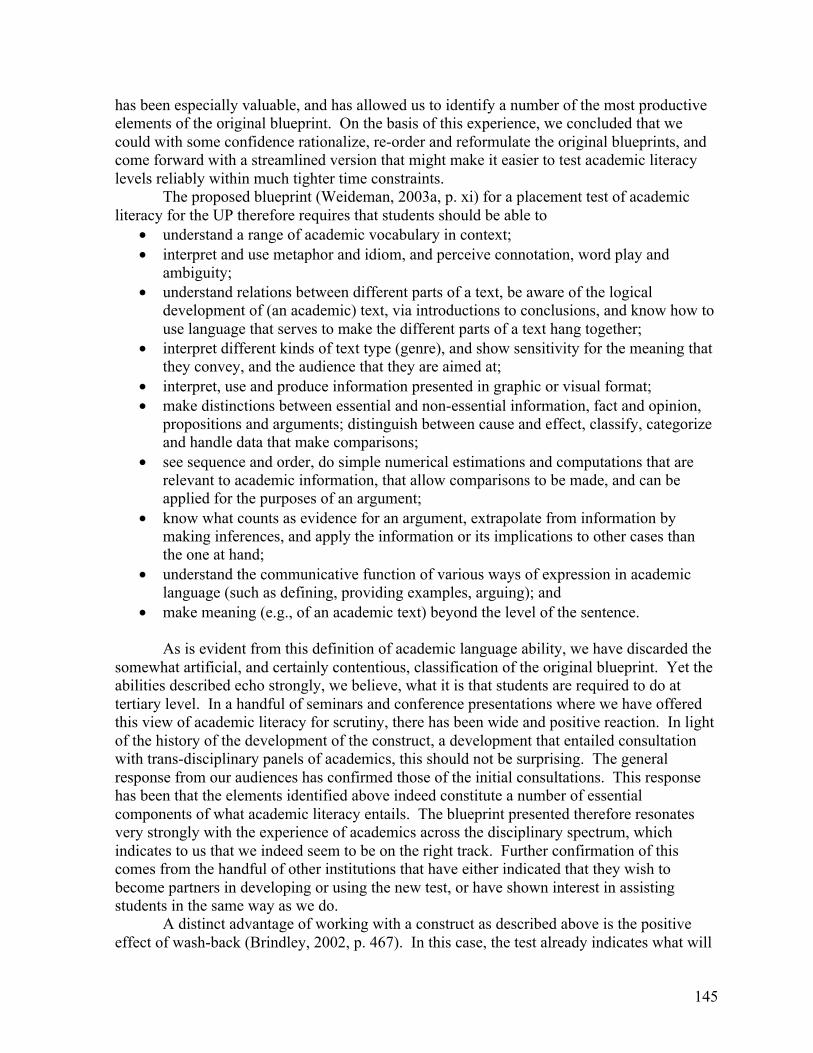
145

has been especially valuable, and has allowed us to identify a number of the most productive elements of the original blueprint. On the basis of this experience, we concluded that we could with some confidence rationalize, re-order and reformulate the original blueprints, and come forward with a streamlined version that might make it easier to test academic literacy levels reliably within much tighter time constraints.

The proposed blueprint (Weideman, 2003a, p. xi) for a placement test of academic literacy for the UP therefore requires that students should be able to

• understand a range of academic vocabulary in context; • interpret and use metaphor and idiom, and perceive connotation, word play and

ambiguity; • understand relations between different parts of a text, be aware of the logical

development of (an academic) text, via introductions to conclusions, and know how to use language that serves to make the different parts of a text hang together;

• interpret different kinds of text type (genre), and show sensitivity for the meaning that they convey, and the audience that they are aimed at;

• interpret, use and produce information presented in graphic or visual format; • make distinctions between essential and non-essential information, fact and opinion,

propositions and arguments; distinguish between cause and effect, classify, categorize and handle data that make comparisons;

• see sequence and order, do simple numerical estimations and computations that are relevant to academic information, that allow comparisons to be made, and can be applied for the purposes of an argument;

• know what counts as evidence for an argument, extrapolate from information by making inferences, and apply the information or its implications to other cases than the one at hand;

• understand the communicative function of various ways of expression in academic language (such as defining, providing examples, arguing); and

• make meaning (e.g., of an academic text) beyond the level of the sentence.

As is evident from this definition of academic language ability, we have discarded the somewhat artificial, and certainly contentious, classification of the original blueprint. Yet the abilities described echo strongly, we believe, what it is that students are required to do at tertiary level. In a handful of seminars and conference presentations where we have offered this view of academic literacy for scrutiny, there has been wide and positive reaction. In light of the history of the development of the construct, a development that entailed consultation with trans-disciplinary panels of academics, this should not be surprising. The general response from our audiences has confirmed those of the initial consultations. This response has been that the elements identified above indeed constitute a number of essential components of what academic literacy entails. The blueprint presented therefore resonates very strongly with the experience of academics across the disciplinary spectrum, which indicates to us that we indeed seem to be on the right track. Further confirmation of this comes from the handful of other institutions that have either indicated that they wish to become partners in developing or using the new test, or have shown interest in assisting students in the same way as we do.

A distinct advantage of working with a construct as described above is the positive effect of wash-back (Brindley, 2002, p. 467). In this case, the test already indicates what will

146

eventually be taught, and the course reflects the construct of the test. This in turn improves the face validity of the test. Since the construct of the test is formulated in terms of a range of outcomes, in line with the outcomes-based approach that is now the convention within higher education in South Africa, it moreover shares with such approaches a number of advantages, such as a “closer alignment between assessment and learning, greater transparency of reporting, and improved communication between stakeholders” (Brindley, 2002, p. 465). The issue of greater transparency is also the foundation of attempts aimed at making the test accountable, a concern that is now widely echoed in the testing literature, and to which we finally turn.

A next challenge is, of course, to find, from the specifications implied in the blueprint above, appropriate task types that reliably measure the academic literacy levels of students in our test population.

From Blueprint to Specification to Item Type The size of the testing populations and the urgency of making the results of the test

known in themselves point to the necessity of employing a multiple choice format (that can be marked electronically), and of exploiting to the full other economical means that may be available. The necessity of using multiple choice questions has forced us, incidentally, to abandon the knee-jerk, normally negative reaction that language educators have with regard to this kind of testing. In being forced to conceive of ways of employing this format, we have become more inventive and creative than we would otherwise have been, if we had simply succumbed to the prejudice that “one cannot test (this or that aspect of) language in this way.” The ingenuity of some of the questions has demonstrated to us that this bias is often exactly that: a prejudice that prevents us from seeking creative solutions. Take, as an example, the following question (based on a reading passage) that was employed to test understanding of metaphor:

We should understand the phrase “milk in their blood” in the first sentence to mean that both men

(a) have rare blood diseases inherited from their parents (b) are soft-spoken, mild-mannered young farmers (c) don’t like to make profit at the expense of others (d) are descended from a long line of dairy farmers

The same applies to the following question, that tests one’s understanding of idiom:

Paragraph 2 speaks of ‘hatching a plan.’ Normally, we would think of the thing that is hatched as

(a) a door (b) a loft (c) a car (d) an egg

Or consider this one, which is designed to test the knowledge of the candidate

regarding what counts as evidence:

147

In the second paragraph, we read that “milk farms have been the backbone of this country” for centuries. Which sentence in the fourth paragraph provides evidence of the claim that it has been so ‘for centuries’?

(a) The first sentence (b) The second sentence (c) The third sentence (d) None of these

As may already be evident from these few examples, the tasks that the test takers are being asked to perform belong to a set of abilities or task types that are much broader in scope than that of a test that defines academic literacy in terms of skills, or reduces it to the mastery of sound, form and meaning.

Test Specifications A first major challenge to test developers is aligning the construct of a test with the

specifications that flow from this framework. Securing this alignment is a significant initial step in ensuring that the test indeed measures what it sets out to measure, i.e., is valid. Specifications can be drawn up in terms of a predetermined format, conceived of in terms that satisfy a range of formal requirements. For example, one may wish to specify, with a view to articulating the construct validity of a test, first the construct or blueprint from which the item type or the item itself is derived. One may add to this the logistical conditions under which the task type or individual item must be administered (pencil and paper mode; electronic format; the need for a sound system or time measurement device), the format of the kind of item, or an exemplification of this format, and so forth. For examples of such specification formats, there is a detailed exposition in Davidson and Lynch’s (2002) Testcraft.

For the sake of brevity, however, and since this is not the main focus of the present discussion, we shall attend here to one aspect only of such item type specifications: that of how they align with a feature or component of the blueprint of our test of academic literacy levels. We therefore tabulate below the sub-components of the test in such a way that they can immediately be related (or not) to the item types that test each language ability specification.

Test Task Types The eventual selection of task types for a particular test depends not only on their

alignment with the blueprint of the test and the specifications that flow from it, but also on the judgment of the test developer as to the productivity of the item type. Thus, the test developer has to make a judgment, either in terms of experience and expectation, or based on some quantitative measure, or on both of these, in respect of each test task type. Broadly, test task types will be adjudged to fall into one of four categories, as shown in Figure 3: acceptable (a high degree of alignment with the test construct, but apparently not productive), unacceptable (low productivity coupled with small degree of alignment with blueprint), desirable (high alignment with construct, as well as productive), or not ideal (potentially productive, but not quite aligned with framework):

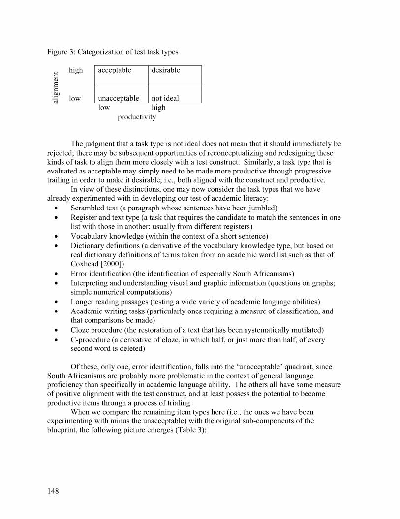
148

Figure 3: Categorization of test task types

alig

nmen

t high acceptable desirable

unacceptable not ideal low

low high productivity

The judgment that a task type is not ideal does not mean that it should immediately be rejected; there may be subsequent opportunities of reconceptualizing and redesigning these kinds of task to align them more closely with a test construct. Similarly, a task type that is evaluated as acceptable may simply need to be made more productive through progressive trailing in order to make it desirable, i.e., both aligned with the construct and productive.

In view of these distinctions, one may now consider the task types that we have already experimented with in developing our test of academic literacy:

• Scrambled text (a paragraph whose sentences have been jumbled) • Register and text type (a task that requires the candidate to match the sentences in one

list with those in another; usually from different registers) • Vocabulary knowledge (within the context of a short sentence) • Dictionary definitions (a derivative of the vocabulary knowledge type, but based on

real dictionary definitions of terms taken from an academic word list such as that of Coxhead [2000])

• Error identification (the identification of especially South Africanisms) • Interpreting and understanding visual and graphic information (questions on graphs;

simple numerical computations) • Longer reading passages (testing a wide variety of academic language abilities) • Academic writing tasks (particularly ones requiring a measure of classification, and

that comparisons be made) • Cloze procedure (the restoration of a text that has been systematically mutilated) • C-procedure (a derivative of cloze, in which half, or just more than half, of every

second word is deleted)

Of these, only one, error identification, falls into the ‘unacceptable’ quadrant, since South Africanisms are probably more problematic in the context of general language proficiency than specifically in academic language ability. The others all have some measure of positive alignment with the test construct, and at least possess the potential to become productive items through a process of trialing.

When we compare the remaining item types here (i.e., the ones we have been experimenting with minus the unacceptable) with the original sub-components of the blueprint, the following picture emerges (Table 3):

149

Table 3. Comparison of Test Specification and Task Type Specification Task type(s) Vocabulary comprehension

Vocabulary knowledge Dictionary definitions Cloze C-procedure

Understanding metaphor & idiom

Longer reading passages

Textuality (cohesion and grammar)

Scrambled text Cloze C-procedure (perhaps) Register and text type Longer reading passages Academic writing tasks

Understanding text type (genre)

Register and text type Interpreting and understanding visual & graphic information Scrambled text Cloze procedure Longer reading passages Academic writing tasks (possibly also) C-procedure

Understanding visual & graphic information

Interpreting and understanding visual & graphic information (potentially:) Longer reading passages

Distinguishing essential/ non-essential

Longer reading passages Interpreting and understanding visual & graphic information Academic writing tasks

Numerical computation

Interpreting and understanding visual & graphic information Longer reading passages

Extrapolation and application

Longer reading passages Academic writing tasks (Interpreting and understanding visual & graphic information)

Communicative function

Longer reading passages (possibly also:) Cloze, Scrambled text

Making meaning beyond the sentence

Longer reading passages Register and text type Scrambled text Interpreting and understanding visual & graphic information

150

It is evident already from this rudimentary classification and comparison of specifications with task types that some task types at least potentially measure academic literacy more productively than others. Why should one then rather not employ those that appear to satisfy more specifications than others? The answer is complex, and opens up an old debate that concerns the quest for a single measure, or at least a very few measures, of language ability, such as in the historical debate on so-called integrative forms of testing (such as cloze, and possibly dictation) versus tests of discrete abilities. The stock answer to this, no doubt, is that while a limited number of sub-tests may be ideal from a test developer’s point of view, it is generally so that the larger the number of sub-tests, the greater the chances are that the instrument will test reliably. For us, however, the reasons for not focusing exclusively on the most productive tasks type(s) are more practical: while it is evident, for example, that a longer reading passage might yield more, and a greater range of information on a candidate’s level of academic literacy, it is also the case that it takes longer for candidates to complete questions that are based on an extended text. In a test that is severely constrained by time, one has to explore other, less time consuming types of task in addition to longer reading passages. Similarly, practical and logistical constraints dictate that, while we may include an academic writing task in a test, its marking must be handled creatively. For example, if we find that the results for the various task types that can be adequately tested in multiple-choice format consistently correlate well (i.e., above 0.85) with the total marks of a test that contains both multiple choice items and others, we may have grounds for deciding to leave the marking of the academic writing task(s) for later, when decisions on borderline cases need to be made.

What we also leave undiscussed for the moment in answering the question relating to the use of more productive types of task, is the relative weight of each specification and, by implication, the test task types that give expression to a specification. We may, for example, wish to assume that in academic language proficiency the understanding of vocabulary generally deserves much greater weight in a test than, say, the understanding of how metaphor and idiom are used by academic authors. Or we might wish to emphasize the importance of distinction-making, which lies at the heart of the academic enterprise, at the expense of a demonstration of the ability to extrapolate, on the assumption that the former ability precedes the latter in the development and socialization of a new entrant into the academic world (and new entrants indeed provide the level at which our academic literacy test is pitched).

What is clear from the provisional alignment above of test task type and test specification is that we need to explore a number of further test task types to satisfy all of the specifications, and that we certainly need to consider making some of the existing test task types more productive. The remainder of this article will focus on how we have developed a format for making one of these task types, cloze procedure, more productive.

A Closer Examination of a Specific Task Type: Text Editing Our interest in this section is on cloze procedure. According to the task type-

specification alignment table in the previous section, cloze is a potentially productive task type because it may test vocabulary, grammar and cohesion, an understanding of text type, and possibly also communicative function. Initial trials that we did with multiple choice cloze (i.e., with a given choice of words that might fill the gaps), however, were disappointing. For example, of the five questions in this task type in a pilot test we ran for 1111 candidates in

151

March 2003, only one made the cut, i.e., had a discrimination index of greater than 0.3, and fitted into the acceptable facility value range we had set, of between 0.3 and 0.7. Only when we relaxed the acceptability criteria to a discrimination index upwards of 0.26 and a facility value of between 0.26 and 0.84, did three of the five items qualify.

Obviously, these values could potentially be improved by, for example, modifying the distracters. But in the meantime, through experience that we had gained in constructing another test, we began to wonder whether we could not also adjust the format of the question. We subsequently designed another task for piloting that not only omitted every 7th word, but also asked of candidates to identify the place where the word had been omitted. Candidates were, therefore, required to select, from the list given, the word that had been omitted, and to indicate its original place. Here is an example:

…The correct answers to the first four (questions 1-8) have been done for you, and are marked in bold in the second and third columns: Text Word Place In 1&2 (a)/ this (b)/ act, (c)/ the (d)/ context otherwise indicates, 3&4(a) / ‘candidate (b)/ means any (c)/ person (d) bound to serve 5&6(a)/articles (b)/of (c)/ clerkship (d)/or to 7&8 (a)/ perform (b)/community (c) / under a contract (d) / of service. It 9&10(a)/ that (b) / irregular (c)/service (d)/ as a 11&12(a)/ candidate (b)/, within (c)/ the (d)/ meaning of 13&14(a)/ the (b)/above, (c)/ is (d)/ irregular service 15&16(a)/ under articles (b)/ or a (c)/ of (d)/ service as defined.

1. (a) if (b) when (c) that (d) unless 3. (a) lawyer (b) attorney (c) conveyancer

(d) paralegal 5. (a) with (b) under

(c) his (d) regular 7. (a) regularly (b) serious (c) service (d) work 9. (a) is (b) concludes

(c) regulates (d) follows 11. (a) paralegal (b) conveyancer

(c) lawyer (d) attorney 13. (a) mentioned (b) definition

(c) construction (d) regulation 15. (a) contract (b) definition

(c) way (d) mode

2. (a)/ (b)/ (c)/ (d)/ 4. (a)/ (b)/ (c)/ (d)/ 6. (a)/ (b)/ (c)/ (d)/ 8. (a)/ (b)/ (c)/ (d)/ 10. (a)/ (b)/ (c)/ (d)/ 12. (a)/ (b)/ (c)/ (d)/ 14. (a)/ (b)/ (c)/ (d)/ 16. (a)/ (b)/ (c)/ (d)/

The results of this 50-item test were encouraging from a number of angles. In the first place, the test developer is always on the lookout for sub-tests that have a reliability measure (alpha) that is higher than that of a whole test, since this is an indication that, in general, this particular kind of test task discriminates not only more reliably, but better and more efficiently than other types of task. This original 50-item pilot on a test group of above

152

average language ability first year students (n = 43) indeed proved slightly (0.8%) more reliable than a previous pilot that also contained 50 items, but in that case spread over seven item or task types.

By eliminating some of the items within the text that did not measure within the desired parameters (i.e., either too low a discrimination value, or too easy or difficult), and by modifying some of the distracters among the remaining items that did not appear to work efficiently, we then came up with a second version of the pilot. Though it used essentially the same text, this version contained only 30 items. It was again trialed on two groups of first year students, the one (n = 21) with lower levels of academic literacy according to another test of academic language proficiency that they had written at the beginning of their studies, the other (n = 23) with higher levels of academic language proficiency according to the same test.

These results were even more encouraging. Table 4 is a comparison of the mean score, reliability (alpha), and average facility value of items (mean percentage correct) of this second version of the test for the two groups. The last column (mean item-total correlation) gives an indication of how, on average, items in the tests discriminate:

Table 4. Initial Reliability and Facility Values Version Ability Mean Alpha Mean % correct Mean item-total

First above average 64.42% 0.749 64 0.232 Second above average 66.96% 0.817 67 0.361

Second below average 58.57% 0.810 59 0.325

As is evident, the improvement of the second version on the first is marked (just in terms of reliability: 9% and 8%, respectively). These results therefore certainly seem to indicate that this particular modification of cloze procedure has promise, and that its productivity and efficiency need to be exploited further. In fact, in subsequent tests of this type, that were embedded within a longer test of academic literacy for a large group of below average ability students, the results remained equally encouraging, as shown in Table 5. There are, however, some problems that prevent us from exploiting this format fully. Table 5. Further Reliability and Facility Values Version Ability Mean Alpha Mean % correct Mean item-total

Third (English)

below average 48.34% 0.864 48 0.353

Fourth (Afrikaans)

below average 70.191% 0.828 70 0.331

153

Remaining Problems

As with any experimental format, this modified form of cloze procedure still has a number of difficulties that need ironing out before one can recommend it for wider use. Two unanswered questions that remain, simply because we have not yet had the time to experiment more widely, are how to select the right text for our audience, and how to mutilate the text (deleting every 7th word, or less or more frequently). More frequent deletion would, in our judgment, probably make a text too difficult to restore for new entrants into the academic world. Less frequent deletion would solve a number of sheer practical problems (fitting both text and questions into three narrow columns).

The most vexing problem, however, is how to write the rubric so that it is clear and intelligible. Acting on advice from some of the test administrators in our first two rounds of pilots, we have now, in a third pilot with another (probably easier) text, changed the second and third columns of the original around, and re-written the instruction, as follows: Text Editing

Some words are missing from the text below. In this task, you have to restore the text in the first column to its original form. To do so, you first select a place [marked (a)/, (b)/, (c)/ or (d)/ in the text, with the question numbers in the second column] where you think the word is missing in the text. Then you select a word [(a), (b), (c) or (d)] from those in the third column to complete the text. Mark the correct answers on your answer sheet. The unevenly numbered questions (65, 67, 69, 71, etc.) are for the place, the evenly numbered ones (66, 68, 70, 72, etc.) for the word you have selected to fill in. The correct answers to the first three have been done for you, and are marked in bold in the second and third columns.

We are not entirely convinced that the advice we took (of switching the columns) was

the best: candidates still find this too difficult, and too many in the third round of piloting asked for an explanation. If they were more familiar with the format, they would probably not have needed an additional explanation. In the meantime, however, we still need to devise a way, either by rewriting the rubric in more intelligible language, or by making another plan altogether, of really making a promising task type work. In that way, a type of task that started out, in terms of our matrix above, as ‘not ideal,’ can gravitate first towards ‘acceptable’ and, finally, the ‘desirable’ part of the quadrant.

Conclusion and the Way Forward

In this paper, the focus was on the reasons for switching constructs in the context of testing academic literacy levels, initially within one specific institution, but eventually in a good number of generally similar institutions. It represents an attempt to clarify and contextualize the conceptualisation of a test, in the spirit of Shohamy’s (2001) encouragement to language testers to examine every result of a test, and to re-appraise each foreseeable implication. In order to be accountable in any applied linguistic endeavour (Weideman,

154

2003b), as this era of greater transparency demands from all institutions that wield power, it is essential that one begins by telling the story of the main instruments of exercising that power, in this case: a test. The wide interest that the new test has already engendered among other higher education institutions in South Africa means that it will not be confined to a single, local context, and that its power to affect the lives of larger numbers of students may certainly be greater than initially envisaged. This alone should make a public (South African) description of how the test has been conceptualised essential.

The proof, however, is in the pudding. The second part of this paper was mainly devoted to an experiment focusing on cloze procedure. The task type was described and problems were outlined.

The most exciting phase still lies ahead, when the 2004 intake (approximately 7000) will sit this test of academic literacy levels in January 2004. The results will be analysed statistically and validation studies will be conducted throughout 2004. The test will also be assessed in terms of the extent to which it reflects the new construct.

Acknowledgments

I would like to extend my sincere gratitude towards the staff of the English Language Institute, University of Michigan, for their assistance and guidance especially during my visit to the ELI in April 2003. Also, I would like to thank my supervisor, Prof. Albert Weideman, for his guidance and assistance in the execution of this project.

References Bachman, L. F., & Palmer, A. S. (1996). Language testing in practice: Designing and

developing useful language tests. Oxford: Oxford University Press. Blanton, L. L. (1994). Discourse, artifacts and the Ozarks: Understanding academic literacy.

Journal of Second Language Writing, 3(1), 1-16. Brindley, G. (2002). Issues in language assessment. In R.B. Kaplan (Ed.). The Oxford

handbook of applied linguistics (pp. 459-470). Oxford: Oxford University Press. Butler, G., & van Dyk, T. (July, 2003). A language support course in academic English for

first year engineering students at the University of Pretoria. Paper presented at the 2003 Federation des Professeurs de Langues Vivantes conference, Rand Afrikaans University.

Cooper, P., & van Dyk, T. (2003). Measuring vocabulary: A look at different methods of vocabulary testing. Perspectives in Education, 21(1), 67-80.

Coxhead, A. (2000). A new academic word list. TESOL Quarterly, 34(2), 213-238. Davidson, F., & Lynch, B. K. (2002). Testcraft. New Haven, CT: Yale University Press. Davies, A., Brown A., Elder C., Hill K., Lumley T., & McNamara T. (1999). Dictionary of

language testing. Cambridge: Cambridge University Press. Douglas, D. (2000). Assessing languages for specific purposes. Cambridge: Cambridge

University Press. Gee, J. P. (1998). What is literacy? In V. Zamel & R. Spack (Eds.). Academic literacies: An

introduction to the issues (pp. 51-59). Mahwah, NJ: Lawrence Erlbaum. Halliday, M. A. K. (1978). Language as social semiotic. London: Edward Arnold.

155

Halliday, M. A. K. (1985). An introduction to functional grammar. London: Edward Arnold. Hjelmslev, L. (1961). Prolegomena to a theory of language (F.J. Whitfield, Trans.). Madison,

WI: The University of Wisconsin Press. Hymes, D. H. (1971). On communicative competence. In J. B. Pride & J. Holmes (Eds.).

Sociolinguistics: Selected readings (pp. 269-293). Harmondsworth, UK: Penguin. Searle, J. R. (1969). Speech acts: An essay in the philosophy of language. London: Cambridge

University Press. Shohamy, E. (2001). The power of tests: A critical perspective on the uses of language tests.

Harlow, Essex: Pearson Education. Van Rensburg, C., & Weideman, A. J. (2002). Language proficiency: Current strategies,

future remedies. SAALT Journal for language teaching 36(1 & 2), 152-164. Weideman, A.J. (1981). Systematic concepts in linguistics. Unpublished master’s thesis,

University of the Free State, Bloemfontein, South Africa. Weideman, A.J. (2003a). Academic literacy: Prepare to learn. Pretoria, South Africa: Van

Schaik. Weideman, A.J. (2003b). Towards accountability: A point of orientation for post-modern

applied linguistics in the third millennium. Literator, 24(1), 1-20. Weideman, A.J. (in press). Justifying course and task construction: Design considerations for

language teaching. Acta Academica. Wilkins, D.A. (1976). Notional syllabuses: A taxonomy and its relevance to foreign language

curriculum development. Oxford: Oxford University Press.

156