Planning with Continuous Actions in PartiallyObservable Environments

Matthijs T. J. Spaan and Nikos VlassisInformatics Institute, University of Amsterdam

Kruislaan 403, 1098 SJ Amsterdam, The Netherlands{mtjspaan,vlassis}@science.uva.nl

Abstract— We present a simple randomized POMDP al-gorithm for planning with continuous actions in partiallyobservable environments. Our algorithm operates on a set ofreachable belief points, sampled by letting the robot interactrandomly with the environment. We perform value iterationsteps, ensuring that in each step the value of all sampled beliefpoints is improved. The idea here is that by sampling actionsfrom a continuous action space we can quickly improve thevalue of all belief points in the set. We demonstrate theviability of our algorithm on two sets of experiments: oneinvolving an active localization task and one concerning robotnavigation in a perceptually aliased office environment.

I. INTRODUCTION

Planning is a central problem in robotics: it involvescomputing a sequence of actions that accomplish a taskas effectively as possible. Classical motion planning [1]for instance computes a series of motor commands whichwill move a robot to a desired location. In this paper wespecifically focus on planning for robots which have a con-tinuous set of actions at their disposal. Example scenariosinclude navigating to an arbitrary location, or rotating apan-and-tilt camera at any desired angle. Moreover, in thetype of domains we are considering the robot is uncertainabout the exact effect of its action; it might for instanceend up at a different location than it aimed for, because oferrors in the robot motion. Furthermore, in most realisticscenarios the robot cannot determine with full certaintythe true state of the environment with a single sensorreading, i.e., the environment is only partially observableto the robot. Not only are its sensors likely to sufferfrom noise, the robot’s environment is often “perceptuallyaliased”. This phenomenon occurs when different parts ofthe environment appear similar to the sensor system of therobot, but require different actions.

Partially observable Markov decision processes(POMDPs) provide a rich mathematical frameworkfor acting optimally in such partially observableenvironments [2]. The POMDP defines a sensor modelspecifying the probability of observing a particular sensorreading in a specific state and a stochastic transitionmodel which captures the uncertain outcome of executingan action. The robot’s task is defined by the reward itreceives at each time step, and its goal is to maximizethe discounted cumulative reward it gathers. Assuming a

discrete state space, the POMDP framework allows forcapturing all uncertainty introduced by the transition andobservation model by defining and operating on the beliefstate of a robot. A belief state is a probability distributionover all states and summarizes all information regardingthe past.

Computing optimal planning solutions for POMDPs isan intractable problem for any reasonably sized task [3],[4], calling for approximate solution techniques [5], [6]. Arecent line of research on approximate POMDP algorithmsfocuses on the use of a sampled set of belief points onwhich planning is performed [6], [7], [8], [9], [10], [11].The idea is that instead of planning over the completebelief space of the robot (which is intractable for largestate spaces), planning is carried out only on a limitedset of prototype beliefs that have been sampled by lettingthe robot interact (randomly) with the environment. Thecomputed policy generalizes over the complete belief spacevia a set of hyperplanes that cause nearby beliefs to sharethe same policy.

In previous work [10] we developed a simple random-ized point-based POMDP algorithm called PERSEUS. Weapplied it to robotic planning problems featuring large statespaces and high dimensional observations, but with discreteaction spaces. In PERSEUS we perform value iterationsteps, ensuring that in each step the value of all sampledbelief points is improved, by only updating the value and itsgradient of a randomly selected subset of points. Extendingthis scheme, we propose in this paper CA-PERSEUS, analgorithm for planning with continuous actions in partiallyobservable environments, which is particularly relevant inrobotics. Obviating the need to discretize a robot’s actionspace allows for more precise control. Most work onPOMDP solution techniques targets discrete action spaces.Exceptions include the application of a particle filter to acontinuous state and action space [12] and certain policysearch methods [13]. We report on experiments in an ab-stract active localization domain in which a robot can con-trol its range sensors to influence its localization estimate,and on results from a navigation task involving a mobilerobot with omnidirectional vision in a perceptually aliasedoffice environment. We will demonstrate that CA-PERSEUScan compute successful policies for these domains.

II. POMDP PLANNING

We start by reviewing briefly the POMDP frameworkfrom a robotic point of view, followed by techniques to(approximately) solve POMDPs. The POMDP frameworkallows one to define a task for a robot with noisy sensorsand stochastic actions. At any time step the environmentis in a state s ∈ S. A robot inhabiting this environmenttakes an action a ∈ A and receives a reward r(s, a) fromthe environment as a result of this action. The environmentswitches to a new state s′ according to a known stochastictransition model p(s′|s, a). The transition model is oftenassumed Gaussian when a is a movement action, reflectingerrors in the robot motion. The robot then perceives anobservation o ∈ O that depends on its action. This obser-vation provides the robot with information about the states′ through a known stochastic observation model p(o|s, a).The observation model captures the sensory capabilitiesof the robot. The sets S, O and A are assumed discreteand finite here, but we will generalize to continuous A inSection III.

In order for a robot to choose its actions successfullyin such a partially observable environment some form ofmemory is needed. In belief based POMDP solving wemaintain a discrete probability distribution b(s) over statess that summarizes all information about the past. Thisdistribution, or belief, is a Markovian state signal and canbe updated using Bayes’ rule each time the robot takes anaction a and receives an observation o, as follows:

boa(s′) =

p(o|s′, a)

p(o|a, b)

∑

s∈S

p(s′|s, a)b(s), (1)

where p(o|a, b) =∑

s′∈S p(o|s′, a)∑

s∈S p(s′|s, a)b(s) isa normalizing constant.

Given such a belief space, the planning task becomesone of computing an optimal policy, a mapping frombeliefs to actions that maximizes the expected discountedfuture reward of the robot E[

∑∞t γtr(st, at)], where γ is

a discount rate, 0 ≤ γ < 1. A policy can be defined bya value function, which defines the expected amount offuture discounted reward for each belief state. The valuefunction of an optimal policy is called the optimal valuefunction and is denoted by V ∗, which satisfies the Bellmanoptimality equation V ∗ = HV ∗, or

V ∗(b) = maxa∈A

[

∑

s∈S

r(s, a)b(s) + γ∑

o∈O

p(o|a, b)V ∗(boa)

]

,

(2)with bo

a given by (1), and H is the Bellman backupoperator [14]. When (2) holds for every b in the beliefspace we are ensured the solution is optimal.

A. Value iteration in POMDPs

A classical method for solving POMDPs is value iter-ation. This method iteratively builds better estimates ofV ∗ by applying the operator H to an initially piecewise

linear and convex value function V0 [15]. The intermediateestimates V1, V2, . . . will then also be piecewise linear andconvex. We will throughout assume that a value functionVn at step n is represented by a finite set of vectors(hyperplanes) {α1

n, α2n, . . .}. Additionally, with each vector

an action a(αin) ∈ A is associated, which is the optimal

one to take in the current step, assuming optimal actions areexecuted in following steps. Given a set of vectors {αi

n}|Vn|i=1

in Vn, the value of a belief b is given by

Vn(b) = max{αi

n}i

b · αin, (3)

where (·) denotes inner product. The gradient of the valuefunction at b is given by the vector αb

n = arg max{αin}i

b ·

αin, and the policy at b is given by π(b) = a(αb

n).The main idea behind many value iteration algorithms

for POMDPs is that for a given value function Vn and aparticular belief point b we can easily compute the vectorαb

n+1 of HVn such that

αbn+1 = arg max

{αin+1

}i

b · αin+1 (4)

where {αin+1}i is the (unknown) set of vectors for HVn.

We will denote this operation α = backup(b). It computesthe optimal vector for a given belief b by back-projectingall vectors in the current horizon value function one stepfrom the future and returning the vector that maximizesthe value of b. In particular, defining ra(s) = r(s, a), itis straightforward to show that combining (1), (2), and (3)gives [11]:

Vn+1(b) = maxa

[

b · ra + γ∑

o

max{gi

a,o}i

b · gia,o

]

, with (5)

gia,o(s) =

∑

s′

p(o|s′, a)p(s′|s, a)αin(s′). (6)

Applying the identity maxj b·αj = b·arg maxj b·αj in (5)twice, we can compute the vector backup(b) as follows:

backup(b) = arg max{gb

a}a∈A

b · gba, with (7)

gba = ra + γ

∑

o

arg max{gi

a,o}i

b · gia,o. (8)

Note that the backup operator in (7) requires enumeratingall actions, which is not feasible in practice when the actionspace is continuous.

Although computing the vector backup(b) for a givenb is straightforward, locating all vectors ∪bbackup(b) ofHVn typically requires linear programming and is thereforecostly in high dimensions [2]. A promising way to sidestepthis issue is to sample in advance a set of belief pointsfrom the belief simplex, and then perform value updateson these points only [5], [6], [7], [9], [10], [11]. Point-based solution techniques are justified by the fact that inmost robotic problem settings the belief simplex is sparse,in the sense that only a limited number of belief points

can ever be reached when the robot directly interacts withthe environment. In these cases, one would like to planonly for those reachable beliefs instead of planning overthe complete belief simplex.

In [10] we described PERSEUS, a simple approximatepoint-based algorithm for solving POMDPs which we haveapplied to robotic planning. The key idea is that, in eachvalue iteration step, we can improve the value of all pointsin the belief set by only updating the value and its gradientof a randomly selected subset of the points. We performedexperiments in benchmark problems from literature, andPERSEUS turns out to be very competitive to state-of-the-art methods in terms of solution quality and computationtime. We show here that this scheme of ‘partial’ valueupdates is also very well suited for handling problems withcontinuous action spaces.

III. PLANNING WITH CONTINUOUS ACTIONS

In [10] our PERSEUS POMDP algorithm assumed dis-crete action sets. Here we extend PERSEUS to handle prob-lems with continuous action spaces. Instead of consideringa finite and discrete action set A we parameterize therobot’s actions on a set of k, problem-specific parametersθ = {θ1, θ2, . . . , θk}. These parameters are real valued andcan for instance denote the angle by which the robot ro-tates. Computing a policy containing such actions requiresmodifying the backup operator defined in Section II-A,since A now contains an infinite numbers of actions (andtherefore maximization over these is not straightforward).The idea here is that instead of maximizing over all a ∈ A,we sample actions at random from A, compute their backedup vectors, and check whether one of the resulting vectorsimproves the value of the corresponding belief point. Thebackup operator as defined in (7) is replaced by a backupoperator α = backup′(b):

backup′(b) = arg max{gb

a}a∈A′

b

b · gba, with (9)

A′b = {ai : ai is drawn from A}, (10)

and gba as defined in (8). We draw at random a set A′

b fromthe continuous set A, in particular specific θ vectors whichdefine actions and which in turn define the gb

a vectors. Wecan easily incorporate such a backup operator in PERSEUSas we will show next.

We first let the robot randomly explore the environmentand collect a set B of reachable belief points. Our CA-PERSEUS algorithm performs a number of backup stages.In each backup stage, given a value function Vn, wecompute a value function Vn+1 that improves the valueof all b ∈ B. Often, a small number of vectors will besufficient to improve Vn(b) ∀b ∈ B (especially in the firststeps of value iteration), and we compute these vectorsin a randomized greedy manner by sampling from B. Weinitialize the value function V0 as a single vector with allits components equal to 1

1−γmins,a r(s, a) [16]. Starting

with V0, we perform a number of value function updatestages until convergence (which is guaranteed [11], [7]).In particular, given Vn, a backup stage is as follows:

CA-PERSEUS backup stage

1) Set Vn+1 = ∅. Initialize B = B.2) Sample a belief point b uniformly at random from B

and compute α = backup′(b).3) If b · α ≥ Vn(b) then add α to Vn+1, otherwise add

α′ = arg maxα∈Vnb · α to Vn+1.

4) Compute B = {b ∈ B : Vn+1(b) < Vn(b)} . IfB = ∅ then stop, otherwise go to 2.

The algorithm tries in each backup stage to improve thevalue of all points in B (step 4). If some points are notimproved yet (set B), one of them is selected at randomand a corresponding vector is generated (step 2). If thevector improves the value of the selected point b we add itto Vn+1 and update Vn+1(b) for all b ∈ B. If not, weignore the vector and insert a copy of the maximizingvector of b from Vn in Vn+1. Adding a vector improvesthe value of hopefully many non-improved points, and theprocess continues until all points are improved. Essentiallyour value update scheme defines an approximate Bellmanbackup operator that improves (instead of maximizes) thevalue of all belief points in each iteration, and turns out tobe very successful in practice. It is exactly this “improve-only” principle that justifies the use of the randomizedoperator backup′ (9) in step 2 of the algorithm insteadof the deterministic operator backup (7).

An alternative to sampling for handling continuousaction spaces is to discretize the action space. A com-putational advantage of reducing the action space to aset of discrete actions is the fact that when A is smallenough one can cache in advance the explicit tabularrepresentation of the transition, observation and rewardmodels for all a ∈ A. In contrast, when we sample areal-valued action we have to generate from a parametricdescription of these models their tabular representation,necessary for computing (6). However, discretization hasits limits, particularly when considering scalability. Thenumber of discrete actions grows exponentially with k,the number of dimensions of θ. For instance, consider arobotic arm with a large number of joints or, as in one ofthe experiments below, a robot which can control a numberof sensors at the same time: discretization would require anumber of bins that is exponential in the number of jointsor sensors, respectively. Furthermore, the discretization canlead to worse control performance, as demonstrated in thesecond set of experiments. Clearly, working directly withcontinuous actions allows for more precise control.

IV. EXPERIMENTS

We applied our algorithm in two domains: an abstractactive localization domain in which a robot can control its

PSfrag replacements

reward

-1

-4

-6

-8

-10

-12

-14

-16

-18

-20

0

0.2

0.4

0.5

0.6

0.8

1

1.2

1.4

1.5

1.6

1.8

2

2.5

3

3.5

4

5

8

10

20

40

50

60

80

100

120

140

150

160

200

400

500

600

800

1000

1200

1400

1500

1600

1800

2000

2500

3000

4000

6000

8000

10000

C

Vtime (s)

∆π

# of vectors

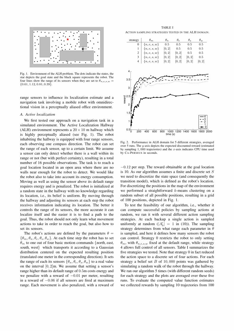
Fig. 1. Environment of the ALH problem. The dots indicate the states, thestar depicts the goal state and the black square represents the robot. Thefour lines show the range of its sensors when they are set to θn,e,s,w ={0.61, 1.12, 0.81, 0.39}.

range sensors to influence its localization estimate and anavigation task involving a mobile robot with omnidirec-tional vision in a perceptually aliased office environment.

A. Active localization

We first tested our approach on a navigation task in asimulated environment. The Active Localization Hallway(ALH) environment represents a 20× 10 m hallway whichis highly perceptually aliased (see Fig. 1). The robotinhabiting the hallway is equipped with four range sensors,each observing one compass direction. The robot can setthe range of each sensor, up to a certain limit. We assumea sensor can only detect whether there is a wall within itsrange or not (but with perfect certainty), resulting in a totalnumber of 16 possible observations. The task is to reach agoal location located in an open area where there are nowalls near enough for the robot to detect. We would likethe robot also to take into account its energy consumption.Moving as well as using the sensor above its default rangerequires energy and is penalized. The robot is initialized ata random state in the hallway with no knowledge regardingits location, i.e., its belief is uniform. By moving throughthe hallway and adjusting its sensors at each step the robotreceives information indicating its location. The better itcontrols the range of its sensors, the more accurate it canlocalize itself and the easier it is to find a path to thegoal. Thus, the robot should not only learn what movementactions to take in order to reach the goal, but also how toset its sensors.

The robot’s actions are defined by the parameters θ ={θm, θn, θe, θs, θw}. At each time step the robot has to setθm to one out of four basic motion commands {north, east,south, west} which transports it according to a Gaussiandistribution centered on the expected resulting position(translated one meter in the corresponding direction). It setsthe range of each its sensors {θn, θe, θs, θw} to a real valueon the interval [0, 2]m. We assume that setting a sensor’srange higher than its default range of 0.5m costs energy andwe penalize with a reward of −0.01 per meter, resultingin a reward of −0.06 if all sensors are fired at maximumrange. Each movement is also penalized, with a reward of

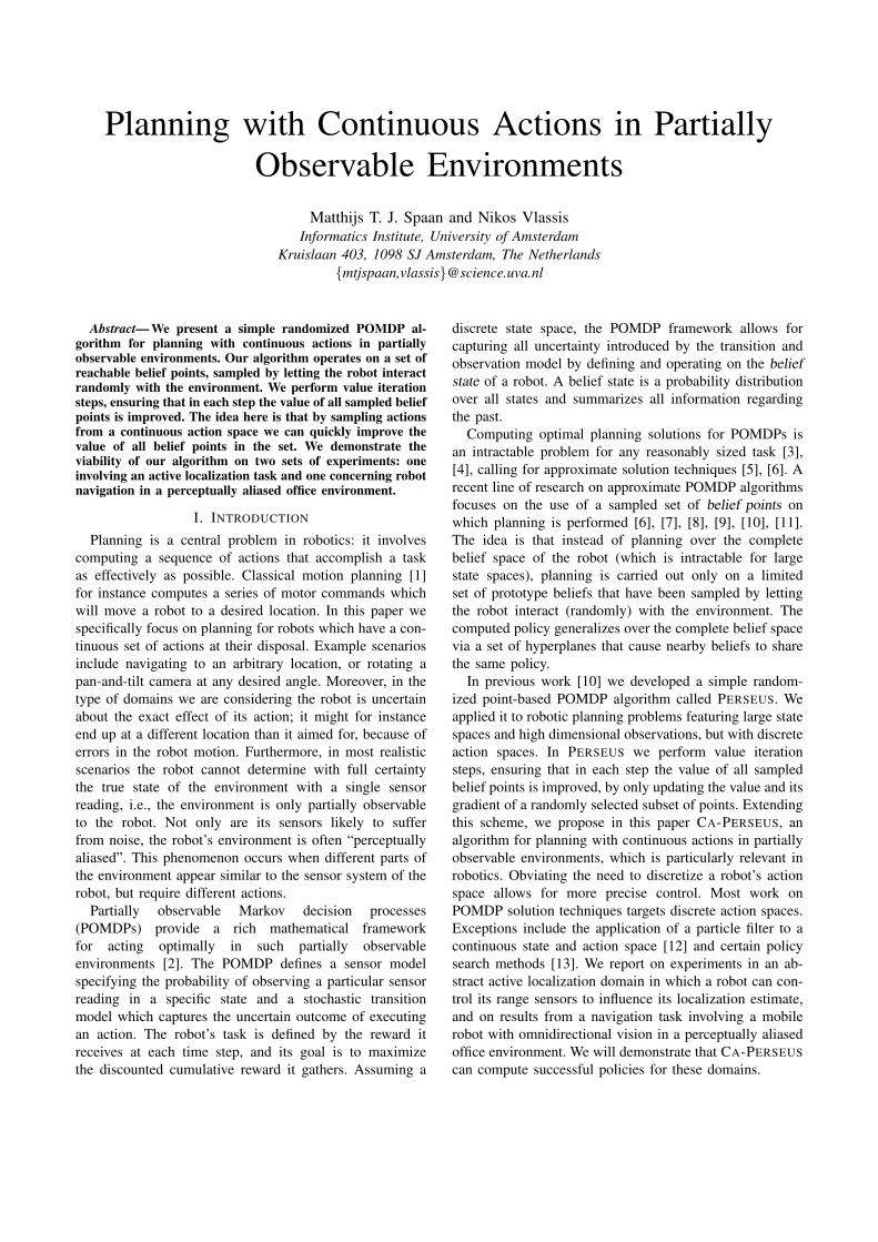
TABLE IACTION SAMPLING STRATEGIES TESTED IN THE ALH DOMAIN.

strategy θm θn θe θs θw

0 {n, e, s, w} 0.5 0.5 0.5 0.5

1 {n, e, s, w} [0, 2] 0.5 0.5 0.5

2 {n, e, s, w} [0, 2] [0, 2] 0.5 0.5

3 {n, e, s, w} [0, 2] [0, 2] [0, 2] 0.5

4 {n, e, s, w} [0, 2] [0, 2] [0, 2] [0, 2]

PSfrag replacements

rew

ard

-1

-4

-6

-8

-10

-12

-14

-16

-18

-20

0

0

0.2

0.4

0.5

0.6

0.8

1

1.2

1.4

1.5

1.6

1.8

2

2.5

3

3.5

4

5

8

10

20

40

50

60

80

100

120

140

150

160

200 400

500

600 800 1000 1200 1400

1500

1600 1800 2000

2500

3000

4000

6000

8000

10000

C

V

time (s)

∆π

# of vectors

4

4

3.5

3

3

2.5

2

2

1.5

11

0.5

Fig. 2. Performance in ALH domain for 5 different strategies, averagedover 5 runs. The y-axis depicts the expected discounted reward (estimatedby sampling 1, 000 trajectories) and the x-axis indicates CPU time usedby CA-PERSEUS in seconds.

−0.12 per step. The reward obtainable at the goal locationis 10. As our algorithm assumes a finite and discrete set S

we need to discretize the state space (and consequently thetransition model), which is defined as the robot’s location.For discretizing the positions in the map of the environmentwe performed a straightforward k-means clustering on arandom subset of all possible positions, resulting in a gridof 100 positions, depicted in Fig. 1.

To test the feasibility of our algorithm, i.e., whether itcan compute successful policies by sampling actions atrandom, we ran it with several different action samplingstrategies. At each backup a single action is sampleduniformly at random (|A′

b| = 1 in (10)). The samplingstrategy determines from what range each parameter in θ

is sampled, and here it defines how many sensors the robotcan control. Strategy 0 restricts the robot to only settingθm, with θn,e,s,w fixed at the default range, while strategy4 allows full control of all sensors. Table I summarizes thefive strategies we tested. Note that strategy 0 in fact reducedthe action space to a discrete set of four actions. For eachstrategy a belief set B of 10, 000 points was gathered bysimulating a random walk of the robot through the hallway.We ran our algorithm 5 times (with different random seeds)for each strategy and the plots are averaged over these fiveruns. To evaluate the computed value function estimateswe collected rewards by sampling 10 trajectories from 100

PSfrag replacements

reward

-1

-4

-6

-8

-10

-12

-14

-16

-18

-20

0

0.2

0.4

0.5

0.6

0.8

1

1.2

1.4

1.5

1.6

1.8

2

2.5

3

3.5

4

5

8

10

20

40

50

60

80

100

120

140

150

160

200

400

500

600

800

1000

1200

1400

1500

1600

1800

2000

2500

3000

4000

6000

8000

10000

C

Vtime (s)

∆π

# of vectors

PSfrag replacements

reward

-1

-4

-6

-8

-10

-12

-14

-16

-18

-20

0

0.2

0.4

0.5

0.6

0.8

1

1.2

1.4

1.5

1.6

1.8

2

2.5

3

3.5

4

5

8

10

20

40

50

60

80

100

120

140

150

160

200

400

500

600

800

1000

1200

1400

1500

1600

1800

2000

2500

3000

4000

6000

8000

10000

C

Vtime (s)

∆π

# of vectors

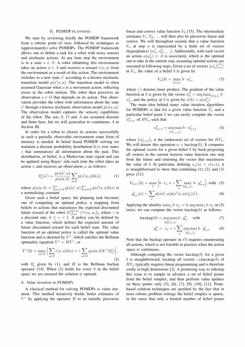
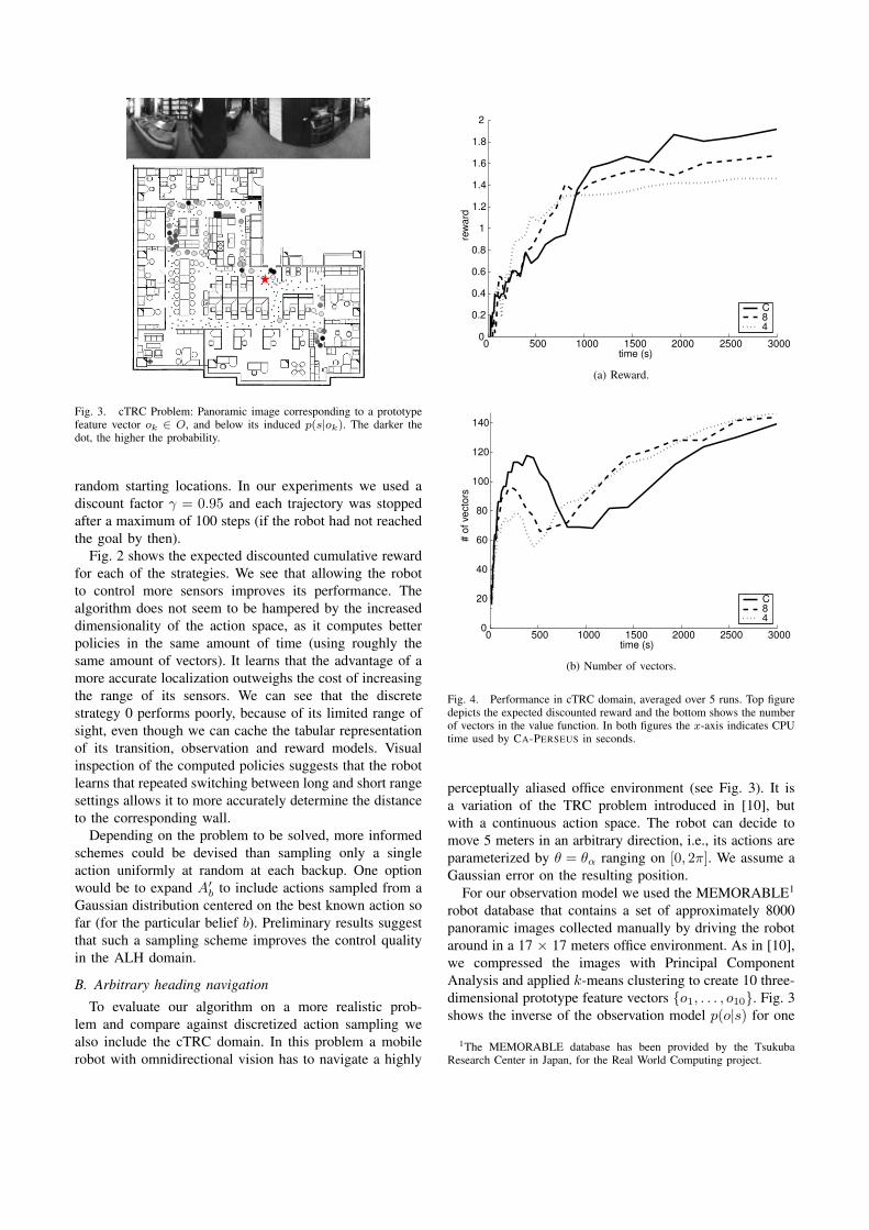
Fig. 3. cTRC Problem: Panoramic image corresponding to a prototypefeature vector ok ∈ O, and below its induced p(s|ok). The darker thedot, the higher the probability.

random starting locations. In our experiments we used adiscount factor γ = 0.95 and each trajectory was stoppedafter a maximum of 100 steps (if the robot had not reachedthe goal by then).

Fig. 2 shows the expected discounted cumulative rewardfor each of the strategies. We see that allowing the robotto control more sensors improves its performance. Thealgorithm does not seem to be hampered by the increaseddimensionality of the action space, as it computes betterpolicies in the same amount of time (using roughly thesame amount of vectors). It learns that the advantage of amore accurate localization outweighs the cost of increasingthe range of its sensors. We can see that the discretestrategy 0 performs poorly, because of its limited range ofsight, even though we can cache the tabular representationof its transition, observation and reward models. Visualinspection of the computed policies suggests that the robotlearns that repeated switching between long and short rangesettings allows it to more accurately determine the distanceto the corresponding wall.

Depending on the problem to be solved, more informedschemes could be devised than sampling only a singleaction uniformly at random at each backup. One optionwould be to expand A′

b to include actions sampled from aGaussian distribution centered on the best known action sofar (for the particular belief b). Preliminary results suggestthat such a sampling scheme improves the control qualityin the ALH domain.

B. Arbitrary heading navigation

To evaluate our algorithm on a more realistic prob-lem and compare against discretized action sampling wealso include the cTRC domain. In this problem a mobilerobot with omnidirectional vision has to navigate a highly

PSfrag replacements

rew

ard

-1

-4

-6

-8

-10

-12

-14

-16

-18

-20

0

0.2

0.4

0.5

0.6

0.8

1

1.2

1.4

1.5

1.6

1.8

2

2.5

3

3.5

4

5

8

10

20

40

50

60

80

100

120

140

150

160

200

400

500

600

800

1000

1200

1400

1500

1600

1800

2000 2500 3000

4000

6000

8000

10000

C

V

time (s)

∆π

# of vectors

2

1.8

1.6

1.4

1.2

1

0.8

0.6

0.4

0.2

00

(a) Reward.

PSfrag replacements

reward

-1

-4

-6

-8

-10

-12

-14

-16

-18

-20

0

0.2

0.4

0.5

0.6

0.8

1

1.2

1.4

1.5

1.6

1.8

2

2.5

3

3.5

4

5

8

10

20

40

50

60

80

100

120

140

150

160

200

400

500

600

800

1000

1200

1400

1500

1600

1800

2000 2500 3000

4000

6000

8000

10000

C

V

time (s)

∆π

#of

vect

ors

140

120

100

80

60

40

20

00

(b) Number of vectors.

Fig. 4. Performance in cTRC domain, averaged over 5 runs. Top figuredepicts the expected discounted reward and the bottom shows the numberof vectors in the value function. In both figures the x-axis indicates CPUtime used by CA-PERSEUS in seconds.

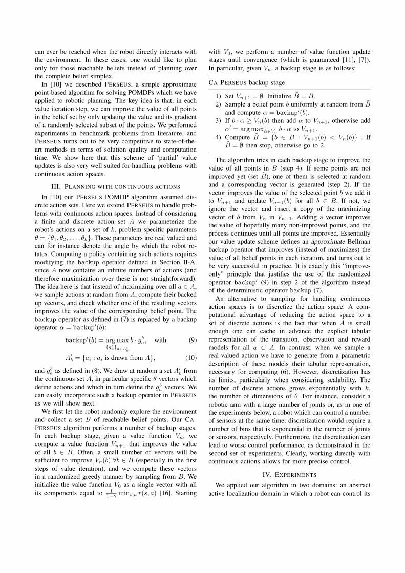
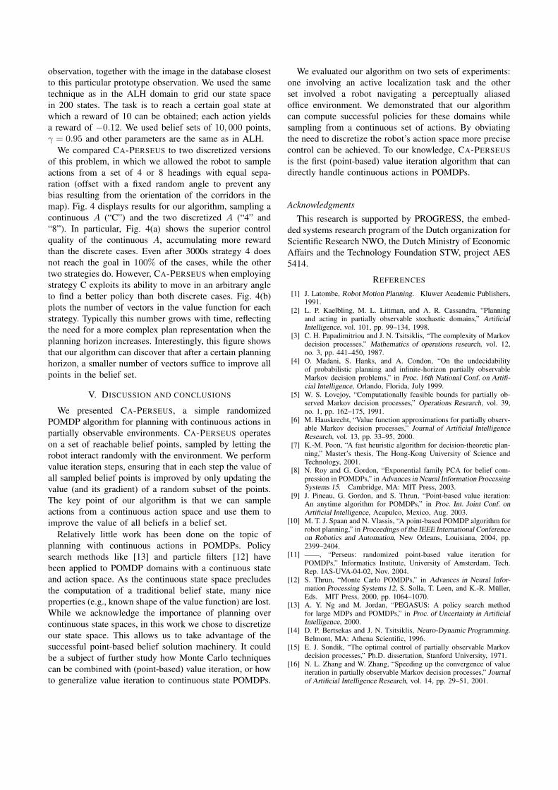
perceptually aliased office environment (see Fig. 3). It isa variation of the TRC problem introduced in [10], butwith a continuous action space. The robot can decide tomove 5 meters in an arbitrary direction, i.e., its actions areparameterized by θ = θα ranging on [0, 2π]. We assume aGaussian error on the resulting position.

For our observation model we used the MEMORABLE1

robot database that contains a set of approximately 8000panoramic images collected manually by driving the robotaround in a 17 × 17 meters office environment. As in [10],we compressed the images with Principal ComponentAnalysis and applied k-means clustering to create 10 three-dimensional prototype feature vectors {o1, . . . , o10}. Fig. 3shows the inverse of the observation model p(o|s) for one

1The MEMORABLE database has been provided by the TsukubaResearch Center in Japan, for the Real World Computing project.

observation, together with the image in the database closestto this particular prototype observation. We used the sametechnique as in the ALH domain to grid our state spacein 200 states. The task is to reach a certain goal state atwhich a reward of 10 can be obtained; each action yieldsa reward of −0.12. We used belief sets of 10, 000 points,γ = 0.95 and other parameters are the same as in ALH.

We compared CA-PERSEUS to two discretized versionsof this problem, in which we allowed the robot to sampleactions from a set of 4 or 8 headings with equal sepa-ration (offset with a fixed random angle to prevent anybias resulting from the orientation of the corridors in themap). Fig. 4 displays results for our algorithm, sampling acontinuous A (“C”) and the two discretized A (“4” and“8”). In particular, Fig. 4(a) shows the superior controlquality of the continuous A, accumulating more rewardthan the discrete cases. Even after 3000s strategy 4 doesnot reach the goal in 100% of the cases, while the othertwo strategies do. However, CA-PERSEUS when employingstrategy C exploits its ability to move in an arbitrary angleto find a better policy than both discrete cases. Fig. 4(b)plots the number of vectors in the value function for eachstrategy. Typically this number grows with time, reflectingthe need for a more complex plan representation when theplanning horizon increases. Interestingly, this figure showsthat our algorithm can discover that after a certain planninghorizon, a smaller number of vectors suffice to improve allpoints in the belief set.

V. DISCUSSION AND CONCLUSIONS

We presented CA-PERSEUS, a simple randomizedPOMDP algorithm for planning with continuous actions inpartially observable environments. CA-PERSEUS operateson a set of reachable belief points, sampled by letting therobot interact randomly with the environment. We performvalue iteration steps, ensuring that in each step the value ofall sampled belief points is improved by only updating thevalue (and its gradient) of a random subset of the points.The key point of our algorithm is that we can sampleactions from a continuous action space and use them toimprove the value of all beliefs in a belief set.

Relatively little work has been done on the topic ofplanning with continuous actions in POMDPs. Policysearch methods like [13] and particle filters [12] havebeen applied to POMDP domains with a continuous stateand action space. As the continuous state space precludesthe computation of a traditional belief state, many niceproperties (e.g., known shape of the value function) are lost.While we acknowledge the importance of planning overcontinuous state spaces, in this work we chose to discretizeour state space. This allows us to take advantage of thesuccessful point-based belief solution machinery. It couldbe a subject of further study how Monte Carlo techniquescan be combined with (point-based) value iteration, or howto generalize value iteration to continuous state POMDPs.

We evaluated our algorithm on two sets of experiments:one involving an active localization task and the otherset involved a robot navigating a perceptually aliasedoffice environment. We demonstrated that our algorithmcan compute successful policies for these domains whilesampling from a continuous set of actions. By obviatingthe need to discretize the robot’s action space more precisecontrol can be achieved. To our knowledge, CA-PERSEUSis the first (point-based) value iteration algorithm that candirectly handle continuous actions in POMDPs.

AcknowledgmentsThis research is supported by PROGRESS, the embed-

ded systems research program of the Dutch organization forScientific Research NWO, the Dutch Ministry of EconomicAffairs and the Technology Foundation STW, project AES5414.

REFERENCES

[1] J. Latombe, Robot Motion Planning. Kluwer Academic Publishers,1991.

[2] L. P. Kaelbling, M. L. Littman, and A. R. Cassandra, “Planningand acting in partially observable stochastic domains,” ArtificialIntelligence, vol. 101, pp. 99–134, 1998.

[3] C. H. Papadimitriou and J. N. Tsitsiklis, “The complexity of Markovdecision processes,” Mathematics of operations research, vol. 12,no. 3, pp. 441–450, 1987.

[4] O. Madani, S. Hanks, and A. Condon, “On the undecidabilityof probabilistic planning and infinite-horizon partially observableMarkov decision problems,” in Proc. 16th National Conf. on Artifi-cial Intelligence, Orlando, Florida, July 1999.

[5] W. S. Lovejoy, “Computationally feasible bounds for partially ob-served Markov decision processes,” Operations Research, vol. 39,no. 1, pp. 162–175, 1991.

[6] M. Hauskrecht, “Value function approximations for partially observ-able Markov decision processes,” Journal of Artificial IntelligenceResearch, vol. 13, pp. 33–95, 2000.

[7] K.-M. Poon, “A fast heuristic algorithm for decision-theoretic plan-ning,” Master’s thesis, The Hong-Kong University of Science andTechnology, 2001.

[8] N. Roy and G. Gordon, “Exponential family PCA for belief com-pression in POMDPs,” in Advances in Neural Information ProcessingSystems 15. Cambridge, MA: MIT Press, 2003.

[9] J. Pineau, G. Gordon, and S. Thrun, “Point-based value iteration:An anytime algorithm for POMDPs,” in Proc. Int. Joint Conf. onArtificial Intelligence, Acapulco, Mexico, Aug. 2003.

[10] M. T. J. Spaan and N. Vlassis, “A point-based POMDP algorithm forrobot planning,” in Proceedings of the IEEE International Conferenceon Robotics and Automation, New Orleans, Louisiana, 2004, pp.2399–2404.

[11] ——, “Perseus: randomized point-based value iteration forPOMDPs,” Informatics Institute, University of Amsterdam, Tech.Rep. IAS-UVA-04-02, Nov. 2004.

[12] S. Thrun, “Monte Carlo POMDPs,” in Advances in Neural Infor-mation Processing Systems 12, S. Solla, T. Leen, and K.-R. Muller,Eds. MIT Press, 2000, pp. 1064–1070.

[13] A. Y. Ng and M. Jordan, “PEGASUS: A policy search methodfor large MDPs and POMDPs,” in Proc. of Uncertainty in ArtificialIntelligence, 2000.

[14] D. P. Bertsekas and J. N. Tsitsiklis, Neuro-Dynamic Programming.Belmont, MA: Athena Scientific, 1996.

[15] E. J. Sondik, “The optimal control of partially observable Markovdecision processes,” Ph.D. dissertation, Stanford University, 1971.

[16] N. L. Zhang and W. Zhang, “Speeding up the convergence of valueiteration in partially observable Markov decision processes,” Journalof Artificial Intelligence Research, vol. 14, pp. 29–51, 2001.