I

I •

-

()

0 • •

, ,t

(t) rJ

r-t-~~

0 = ~

I I

The Collection X

Editor: Dr. lrene Sciriha

Assistant Editor: lan G. Walker

Department of Mathematics

Faculty of Science

University of Malta

Proceedings of Workshop held on Tuesday 16th November 2004

Contents

Foreword

The Collection X Announcement

Teaching mathematics using Excel -Mary Rose Bonello & Silvana Camilleri

A Financial Model -Domnic Cortis

Note on Approximation by Nonlinear Optimization -Dr J aroslav Sklenar

Abelian Sandpiles -Andrew Duncan

Photographs

1

3

4

9

15

24

31

The Collection X 2

Foreward

Is Mathematics a tool? If a tool means an instrument indispensable for the effective, efficient and logical optimisation of the evolution in computer science, physics, chemistry, the natural sciences and the social sciences, then it is a priceless tool to the promoted with care. "Mathematics seems to have almost magical power to predict new phenomena in modern particle physics" according to Jesper Ltzen, professor of the History of Mathematics, at the University of Copenhagen.

In his book, Proofs and Refutations, the mathematical creativity starts with a conjecture, usually suggested by natural occurrences, that need an explanation and may be shown to be UNTRUE by counter examples. This results in a new and finer conjecture after which the process of proofs and refinement is repeated, until a final conjecture is proved true. This research-type dynamic contrasts with the simple cumulative process of mathematics development and paints an essentially internal process. It is an idyllic world that injects energy and inspiration into the creative mathematician. The transfer of the creations and discoveries to the physical world usually takes decades. Why does this breed of mathematicians have in common with painters and engineers like Leonardo da Vinci and Anton Gaudi? I do not need to help the reader to reach conclusions.

Mathematics continually receives apparently insignificant impressions form the outside world that lead to a total decisive path determining the course of science and discoveries. May there be a variety of scientific mathematicians that work on the interface of mathematics and science, accelerating the process translating signals from either field into tangible prototypes.

1. Sciriha Organiser

The Collection X 3

The Collection IX

Faculty of Science

Department of Mathematics

Date: 16th November 2004

Time: 15.00 - 17.00

Venue: MP 316

A seminar/workshop is being held on Tuesday 16th November 2003 at 1500. Students and staff from the Department of Mathematics, Faculty of Science will present ideas from various fields of mathematics.

Keynote speakers:

Dr Jaroslav Sklenar Note on Approximation by Nonlinear Optimization

Mary Rose Bonello Sylvana Camilleri

Teaching Mathematics Using Excel

Andrew Duncan Abelian Sandpiles

Dominic Cortis A Financial Model

We shall end with a brief session for spontaneous problem posing. You are cordially invited to attend.

Abstracts of possible proofs or conjectures which you wish to share with us in this meeting, or in a future one, may be sent to Dr. I. Sciriha or Ms. A. Attard, Department of Mathematics, (marked The Collection), at any time of the year.

Dr. I. Sciriha

Organizer

The Collection X

Teaching Mathematics Using Excel

Mary Rose Bonello & Silvana Camilleri

Introduction

4

'Technology is essential in teaching and learning mathematics; it influences the mathematics that is taught and enhances students' learning.'

(Principles and Standards for School Mathematics-NCTM April 2000)

Aims of using Excel

• Observing patterns and creating sequences

- Sequences

• Seeing connections

- Comparing equations

• Investigating collected data

- Exerting graphs from statistical data

The Collection X 5

Observing Patterns & Creating Sequences

• Excel gives students the opportunity to explore sequences and patterns from a variety of situations

• Observing patterns

- Variables and Function Machines Program

• Creating sequences

- Sequences Program

The Collection X 6

Seeing Connections

• Spreadsheets could be used to help students explore equations and their graphical representations

• See connections between different equations

• Comparing graphs program

The Collection X

Investigating Collected Data

• Spreadsheets could be used

- to display and analyse the collected data

- to simulate randomly occurring events

• Simulf).ting dice program

Simulating the probability of scoring a number with a six-sided dice.

Scores: 532 2 5 4 6 1 1 2 554 1 424 6 1 3 2216562 4 4 3 3 2 2 5 6 1 6 6 2 3 4 522 5 344 2 5 2 5 5 3 6 6 4 2 5 1 3 5 261 1 3 6 3 4 6616466 1 3 2 6 4 541 6 6 5 5 4 5 1 3 1 142 5 5 5 5 5 631 444 4 6 1 4 5 2 2 424 4 2 5 6 5 5 6 1 2 5 4 3 2 3 651 434 6 1 2 4 641 5 1 145

Dice 35

30

25

{2O !15

10

Scores

Press F9togeta new set of throWS]

I Throwsl 150

mean 3.6467 mode 5 median 4 range 5

P(i) 0.1533 P(2) 0.1667 P(3) 0.1067 P(4J 0.2 P(5) 0.2 P(6) 0.17331

7

The Collection X 8

Conclusion

• We have briefly shown how Excel can be a powerful tool during the math­ematics lesson. Still this program cannot be used as an aid for all mathe­matics topics .

• Apart from Excel, one can find other software packages which can be used in the mathematics class, such as:

- Derive

- Cabri Geometry

- MSW Logo

The Collection X 9

A Financial Model Dominic Cortis

This short model sets out a study on a non-existent product which obeys eco­nomic norms. The number of products produced and demand are interdepen­dent in this example and they affect the cost price and selling price which in turn affect the profit. When talking about demand it is important to state the amount of products demanded in a period of time for a given price (for example: The demand for item X is 500 items per week at a selling price of Lm4). In this example, the period of time will be fixed for all cases.

e(l!)

250

200

150

100

50

100 200 300 400 x

Figure 1: Production Cost

The costs of producing an item are classified as both variable and fixed costs. In my first definition of this product I took into consideration variable costs directly related to the production of the item (no transport costs). I wanted this item to cost Lm30 if one is produced and it reaches its optimum cost price (per item) when 100 items are produced and that would be Lm5 per item. So the cost price would diminish up to when 100 items are produced but it starts to increase when producing more than this number. Obviously a quadratic graph would fit this description with its minimum being at x=100. When solving simultaneously an equation c(x) = ax2 + bx + c such that c(l) = 30, c(100) = 5 and c'(100) = 0 it was found that the equation is c(x) - ...l!L X

2 - .§QQQx+ 299005 - 9801 9801 9801 where x represents the number of items produced and c(x) represents the cost price per product. The graph representing this equation is shown in Figure 1.

The Collection X 10

As mentioned above there are also post-production costs and fixed costs -named other costs in this example. Requiring the product to have an initial such cost of Lmll and this diminishing gradually to LmlO and staying at that cost at a certain amount, it was clear that an exponential function was required to dis­play this. The function o(x) = -e1Zo + 10 where o(x) represents other costs (per item) and x represents the number of items produced, shown in Figure 2.

o(x) 11.2

11

10.8

10.6

10.4

10.2

10

9.8 IX

0 50 100 150 200 250 300

Figure 2: Post-Production Cost

There is the common notion that the cheaper an item is the greater is the demand. This is true but not in all cases since even demand has its optimum. The selling price per item changes with respect to the amount of items produced and the cost price. When not considering the cost price, the optimum selling price was to be when 200 items are produced and this would be at Lm 60. Similarly to the production cost price, a quadratic equation was needed and this was found out to be s(x) = - 40100X2 + fox + 50 where s(x) represents the selling price. The graph depicting this quadratic is shown in Figure 3 on Page 11.

The Collection X

sex) 70 60

50 40 30 20 10 o +1 ---,-------,----,-------,--------,

o 100 200 300 400 500 x

Figure 3: Selling price depending on the amount of products produced

11

The selling price was also determined to depend on the cost price such that s(x) = Bf-. So the selling price depends on the items produced and the cost price. This provides room for a 3-D diagram which would be helpful in many cases. The cost price however depends on the number of items produced and thus the above-mentioned 3-D diagram can be set to be a 2-D diagram as illustrated in Figure 4.

Sex)

120 100 80 60 --40 20 0+-----,-----,-----,----,

o 100 200 300 400

x

Figure 4: Selling price of each item depending on number of products produced and the latter's effect on the cost price

The profit per item would then be p(x) = s(x) - c(x) - o(x). The maximum profit per item is reached when 110 items are produced and the profit at this amount is Lm 42.47. The total Profit, denoted q(x), is equal to the profit per item multiplied by the number of items produced. Therefore q(x) = x x p(x). The maximum profit occurs when 153 items are produced at a profit Lm 5693.

The Collection X 12

Similarly the total cost is x x c(x) and the total sales is x x s(x). The graphs denoting these equations are shown in Figures 5 to 8.

45 40 35 30 25 20 15 10 5 0

0

6000

5000

4000

3000

2000

1000

50 100 150 200

Figure 5: Profit per item

O~ \ o 50 100 150 200

Figure 6: Total Profit

250

250

The Collection X 13

90000 80000 70000 60000 50000 40000

30000 20000 10000

0 0 100 200 300 400

Figure 7: Total Cost

25000 ,----------------------------,

20000

15000

10000

5000

o f' o 100 200 300 400

Figure 8: Total Sales

The Collection X 14

The conclusion is not necessarily obtained when the maximum profit is reached. The company that is doing this study may not necessarily have capitalist aims. It might be that it is a government company whose aim is so that the citizens have access to this particular product. Therefore in this case the company is interested in keeping the product selling price as low as possible without making a loss. In another circumstances this company could be a subsidiary and the mother company is only interested in investing a certain amount in it. Therefore it would set the total cost price at a maximum and see the maximum profit given that restriction. The conclusions and needs for this study are infinite and the use of 3-D graphing programs can be used in most cases in order to ease the reaching of a conclusion.

The Collection X

Note on Approximation by Nonlinear Optimization

J aroslav Sklenar Department of Statistics and Operations Research

University of Malta

Introduction

15

The purpose of this note is to discuss the use of nonlinear optimization tech­niques to solve approximation problems typical for example in signal identifi­cation. Different techniques based on classical and modern approaches to time series are available. The presented idea considers cases when signals are com­posed of a finite number of certain nonlinear functions distinct in their param­eter sets, and realization of an additive random error. The focus is given to the sums of parameterized trigonometric functions. As the random error prob­ability distribution is assumed unknown, the common LSQ criterion is replaced with its parameterized generalization. The obtained unconstrained non-smooth minimization problem can be solved either directly or after a smooth reformu­lation to the constrained problem. The initial values for computational pro­cedures are estimated using heuristics and suitable statistical techniques, e.g., periodograms. The ideas are illustrated by simple explanatory examples accom­panied by figures. Test results are shown for MS Excel Solver, MATLAB is used for visualization.

Problem formulation

One of important signal processing tasks is signal identification. We denote x = (Xl, ... , Xn)T a vector of time points (both equidistant and non-equidistant cases are acceptable) and y = (YI, ... , Yn)T a vector of related measurements. Various techniques developed for processing of this type of data may be found. There are approaches based on: analysis of trend and cyclic behaviour, followed by the estimate of random error distribution; analysis of auto correlation structure that leads to advanced autoregressive techniques; and harmonic analysis based on estimates of frequencies. In our case, we assume that n measurements contained in ywere obtained as realizations of the following random vector:

Tt = (Ttl, ... , Ttnf = (t A(xj,(A) + Cj) T ,

k=l j=l, ... ,n

where Cj,j = 1, ... , n denote random errors and functions ik, k = 1, ... , K are of known types, but unknown vectors of parameters i3k> k = 1, ... , K have to

The Collection X 16

be found. Note that the functions fk can be very complex, so the above addi­tive model is in fact no limitation. More complex combinations of individual functions (like product or composed functions) can always be expressed as one complex function.

Harmonic approximation

One of traditional tasks utilizing Fourier series is to identify the signal under the assumption that fk' k = 1, ... , K are trigonometric functions and proportions among unknown frequencies are rational numbers. In this case, the parameters of the following trigonometric function are estimated:

K

Y = L.Bk1 sin(.Bk2x + .Bd· k=l

As usually, we search for coefficients .B k, k = 1, ... , K in such a way to minimize a distance between measurements Y = (Yl, ... , Yn)T and predicted values y = (ih, ... , Yn)T where

K

Yj = L bkl sin(bk2 xj + bk3 )

k=l

and b k , k = 1, ... , K are estimates of unknown .Bk, k = 1, ... , K. A criterion to be minimized can be defined in different ways. We utilize a parametrized distance

n

dp(Y, y) = lIy - Yllp = ~I L IYj - YjIP, j=l

where 0 < p < 00. Therefore, we use (dp(Y, y))pas a criterion to get an uncon­strained optimization problem with unknown variables bk, k = 1, ... , K:

n I K I

P

min{~ Yj - t; bk1 sin(bk2 xj + bd }.

Classical approach to solve this problem is based on the assumption of normal distribution of stochastically independent homoskedastic random errors, and hence p = 2 is used to get the common LSQ (least square) criterion used in regression methods in statistics. An alternative is the direct use of nonlinear optimization algorithms to solve the above minimization problem. The main problem is how to find an optimal solution when the objective function is in general non-differentiable (because of absolute values) and non-convex (because of sin function).

The Collection X 17

Illustration of difficulties

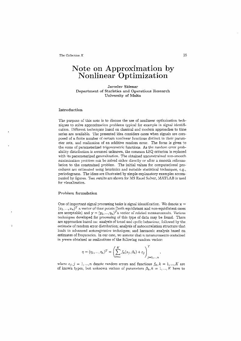
Example 1: The influence of non-convexity, and hence, the importance of suitable choice of the initial solution can be seen from the following example. Figure 1 shows the negative penalty of a harmonic function approximation. The "measurements" were computed by MATLAB [lJ by the formula: y = 0.5sin(x) + 0.2rand - 0.1 (additive uniform noise) in 30 equidistant points in the interval [O,14.5J with the step 0.5 - see the solid line in the Figure 2. The approximation function isy = bI sin(b2x). The mesh is based on a matrix with dimension 100x100 where the parameter bI changed in the interval [-l,lJ with the step 0.02 and the parameter b2 changed in the interval [-l,2J with the step 0.03. The penalty was computed for p=l as the sum of absolute errors. Figure 1 shows the negative penalty, so each peak of the "mountain range" represents one local minimum where the nonlinear programming search algorithm can end. The global minima close to the point bl =0.5, b2 =1 are the two highest peaks. The exact coordinates of the global minimum found by the Excel solver are bl =0.5157, b2=0.9894. The other global minimum is at the same but negative coordinates: sin(x) = -sin(-x). The penalty for this approximation is smaller than the penalty of the original 'ideal' function without noise. Figure 10 shows the original data and two approximations. The correct one corresponds to the global minimum, the wrong one is the left-most local minimum in Figure 9 (exact coordinates bl =0.2699, b2=-0.7081).

The Collection X

Figure 9: Penalty function of harmonic approximation

0.0

04

0.2

o

·0.2

-OA

-0.6

Global and Local minima appro~imation

Figure 10: Harmonic approximation

18

The Collection X 19

Approximation methods

The introduced problem is closely related to the well known area of regression coefficients point estimates in statistics [4]. This widely used technique has com­putational advantages but in certain cases, it is not sufficient. For example it can fail in these cases: unknown random error probability distribution, deviations vary with changing x, and periodogram analysis generally fails for signals that contain close frequencies. In these cases, modern search techniques as genetic algorithms and neural networks are often introduced. These techniques might be slow in finding improved values and their global and local convergence is not guaranteed.

Unconstrained optimization techniques

If the criterion is differentiable (p is even) then the gradient can be computed. However the obtained system of equations is nonlinear and can only exception­ally be solved analytically. Therefore, an iteration procedure based on nonlinear optimization has to be built. If the periodogram identifies one dominating fre­quency, we may decompose the problem complexity starting with K = 1 and the functiony = b1 sin(b2x + b3 ) with three unknown coefficients. In such sim­plest case, the frequency identified by the periodogram is used to initialize b2 •

Then the initial value for b3 is often set to zero and b1 is initially estimated by the LSQ algorithm. Such estimates are often "close enough" to the global opti­mal solutions. Hence, the optimum can be found by efficient locally convergent algorithms.

When p is distinct from 2 (e.g. p = 1), the specialized nonlinear optimization algorithms for LSQ problems, such as the Marquardt - Levenberg algorithm combining the advantages of gradient method robustness and Newton's method speed, cannot be used. Still, fast conjugate directions algorithms may replace them. For example, MS Excel Solver [2] used in the above-mentioned example implements both quasi-Newton and conjugate gradient methods using quadratic approximation for line search. See [3] for details of these methods. Because two choices of approximating gradients numerically are available, the solver is robust enough to successfully deal with non-smooth functions in mid-size problems.

The MS Excel Solver is easy to use, especially for novices in optimization and it supports connection of user-friendly data inputs and graphical outputs. A more experienced users may use similar sophisticated unconstrained optimiza­tion procedures using functions from MATLAB Optimization Toolbox [1].

If the decomposition is not feasible, the previous ideas can still be used for K > 1. However, the problem size and complexity increases and the initial

The Collection X 20

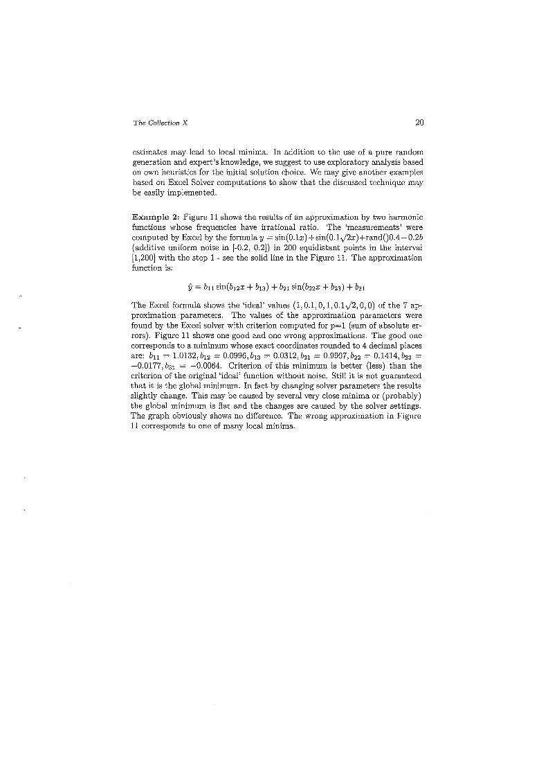
estimates may lead to local minima. In addition to the use of a pure random generation and expert's knowledge, we suggest to use exploratory analysis based on own heuristics for the initial solution choice. We may give another examples based on Excel Solver computations to show that the discussed technique may be easily implemented.

Example 2: Figure 11 shows the results of an approximation by two harmonic functions whose frequencies have irrational ratio. The 'measurements' were computed by Excel by the formula y = sin(O.lx) +sin(0.1y12x)+randOOA-0.2b (additive uniform noise in [-0.2, 0.2]) in 200 equidistant points in the interval [1,200] with the step 1 - see the solid line in the Figure 11. The approximation function is:

fj = bll sin(b12x + b13) + b21 sin(b22x + b23) + b31

The Excel formula shows the 'ideal' values (1,0.1,0,1, 0.1y12, 0, 0) of the 7 ap­proximation parameters. The values of the approximation parameters were found by the Excel solver with criterion computed for p=l (sum of absolute er­rors). Figure 11 shows one good and one wrong approximations. The good one corresponds to a minimum whose exact coordinates rounded to 4 decimal places are: bll = 1.0132, b12 = 0.0996, b13 = 0.0312, b21 = 0.9907, b22 = 0.1414, b23 = -0.0177, b31 = -0.0064. Criterion of this minimum is better (less) than the criterion of the original 'ideal' function without noise. Still it is not guaranteed that it is the global minimum. In fact by changing solver parameters the results slightly change. This may be caused by several very close minima or (probably) the global minimum is fiat and the changes are caused by the solver settings. The graph obviously shows no difference. The wrong approximation in Figure 11 corresponds to one of many local minima.

The Collection X 21

2.5

1.5

0.5

-0.5

-1

-1.5

-2

-2.5

Figure 11: Approximation by two harmonic functions with irrational ratio of frequencies

Example 3: Figure 12 shows the results of an approximation by a sum of a harmonic and a linear functions:

f) = bll sin(b12x + b13 ) + b21 + b22 X

The 'measurements' were originally computed by Excel by the formula: y = 100 sin(0.5x + 3) + 1 + 20x in 15 equidistant points in the interval [1,15] with the step 1. Then the values were manually modified without any clear pattern to simulate for example not accurate measurements - see the solid line in the Figure 4. Note that the reading for x=13 is very far from the original value that may be caused for example by a human error. The Excel formula shows the 'ideal' values (100, 0.5, 3, 1, 20) of the 5 approximation parameters. The values of the approximation parameters were found by the Excel solver. Figure 12 shows two good and one wrong approximations. Note the difference between the criterion computed for p=l (sum of absolute errors) and the criterion computed for p=2 (sum of squared errors). The sum of squares is much more sensitive to excess fluctuations than the sum of absolute errors. Again, the wrong approximation corresponds to one of many local minima.

The Collection X 22

400

350

300

250 ----- Y (p=1)

200 - - - Y (p=2)

150

100

50

0

-50

-100

Figure 12: Approximation by a sum of a harmonic and a linear functions

Unfortunately, unconstrained optimization solvers using approximations of deriva­tives cannot be used in general, as their theoretical properties (guaranteed con­vergence) and numerical behaviour (error influence) can be questionable. There­fore, something more reliable has to be implemented for large-scale problems.

Constrained optimization technique

The above unconstrained minimization problem can be reformulated as a con­strained one with 2 variables associated with each measurement:

n

o < p < 00 : min {L: (dj + djf I dj - d-: = j=l J

K Yj - L: h(Xj, bk ), dj 2: 0, dj 2: 0, j = 1, ... , n}

k=l

Using a suitable algebraic modeling language, the problem can be described using the summation-indexed-based notation.

The Collection X 23

Conclusion

There are non-linear programming software tools based on robust search algo­rithms, often with the possibility to select the one that best suits the problem solved. These tools are general enough, and hence, very flexible in comparison with specialized packages. They can be easily used and require only modest programming abilities if any. Especially, they may serve well in the preparation step when the user identifies the problem features before choosing specialized algorithms and software.

References

[1] MATLAB version 7: User's Guide, The MathWorks Inc., 2004.

[2] MS Excel: Solver's help and documentation, Microsoft, Inc., 2004.

[3] M.S. Bazaraa, H.D. Sherali, and C.M. Shetty, Nonlinear programming: The­ory and algorithms, John Wiley & Sons, 1993.

[4] R.E. Walpole and R.H. Myers, Probability and Statistics for Engineers and Scientists, Prentice Hall, 1993.

[5] R. Fletcher, Practical methods of optimization, John Wiley & Sons, 1990.

The Collection X 24

Abelian Sandpiles Andrew Duncan

• The Abelian Sand pile (AS) is a model originally introduced by physicists to simulate what is known as "self-organized complexity".

• Models exhibiting this phenomenon typically have some form of "avalanche dynamics" , where "stress" is built up until system becomes unstable. On reaching instability, the system reorganizes itself quickly to re-attain sta­bility. Examples are sandpile or avalanche.

• Although the AS is primarily a physical model, it has a very interesting algebraic structure which merits investigation.

The One Dimensional Case

Consider a large table, with n people seated along one side of it. Each person seated at the table holds at most two indistinguishable coins. At each side of the table is a bottomless bin.

Another person (not seated at table) then enters the room, and hands a coin to someone at random. Any person with> 2 coins must give one to the person on the left and one to that on the right. The people at the edges of the table must give one coin to the adjacent person, and throw one in the bin.

Example. Consider the initial configuration 22222. Giving the person on the left edge a coin:

32222 ---t 13222 ---t 21322 ---t 22132 ---t 22213 ---t 22221.

The final configuration is stable in the sense that no person has > 2 coins, thus no further transfer of coins is required.

Representing the current configuration as a mapping T) :{l, ... , n} ---t N then the updating rule can be expressed as:

T) (j) f-- T) (j) - f:.ij

The Collection X 25

where

/:"ij = 2 if i = j } . _ ( 2 -1) /:"ij = -1 if !i - j! = 1 I.e. /:,. - -1 2

The General Sandpile Model

Definition. Let V C Zd be a finite lattice, and V is simply connected. A Toppling Matrix is a !V! x !V! matrix /:,. indexed by x, yE V, with the following properties:

1. For all x, y E V, /:"xx ?::2d, /:"xy ::; 0 for x =I y

2. /:"xy = /:"yx. (Symmetry)

3. I:y/:"xy ?:: 0 (Dissipativity)

4. I:xI:y/:"xy > 0 (Strict Dissipativity)

Definition. A Height Configuration is a function 7] : V -; N where 7](x) is interpreted to be the height (number of grains) at x. Given a toppling matrix /:,., a configuration 7] : is said to be stable if 7](x) ::; /:"xx \:Ix E V. The set of all stable configurations is denoted by n. A node x is s.t.b unstable in 7] if 7] (x ) > /:"xx.

The Toppling Transformation TxO

For x E V, the toppling transformation is a transformation Tx NV -; NV, where

(Tx7])(y) = 7](Y) if x is stable (Tx 7]) (y) = 7] (y) - /:"xy if x is unstable

Due to the dissipativity properties of the toppling matrix, there is always a finite sequence Xl,.' .,xn E V, for which Txl ... Txn7] is stable. Clearly, if x and y are unstable nodes of 7], then TxTy7] = TyTx7]

The Collection X 26

Definition. The Toppling Operator is a function Y : NV -> n defined by

N

Y(7)) = TI Tx,(7)) i=l

where Xl is an unstable vertex of 7), and for any i = 2, ... , N; Xi is unstable in i-I

j[I1 Txj (7)).

Theorem The toppling operator Y is well defined.

Addition Operators

Definition. The addition operator is a map ax : n -> n defined by

aX (7)) = Y(7) + ox).

The addition operator adds a single "grain" to the node X and stabilizes the new (possibly unstable) configuration.

Property 1. ("Closure Relation")

at:.xx = IT a-t:.xy x y

X=FY

Property 2 (Abelian Property)

axay = ayax

The Collection X 27

Recurrent Configurations

There are numerous ways to define recurrent configurations which can be shown to be equivalent. We shall work with the following definition:

Definition. A configuration T) E n is called recurrent if there exist nx :2: 1 such that

IT a~~T) =T).

xEV

The set of recurrent configurations is denoted by R

Is 3t = 0? No.

Let T = I1 ax . Since the set of stable configurations is finite, there must be xEV

some tl < t2 such that TtlT) = T t 2T), and so T t2-

t lTt lT) = TtlT), and thus TtlT)

is recurrent.

Lemma 1. If T) E 3t, then axT) E 3t.

Proof. Follows from Abelian property of addition operator.

Corollary. The maximal configuration '(J, defined by'(J(x) = ~xx is recurrent.

Proof. There is at least one T) E 3t. Obtain the maximal configuration through repeated application of the addition operator. Thus maximal configuration is recurrent by previous lemma.

Define the relation rv on 3t as follows: T) rv e iff::le E NV such that I1 a~(x)T) = e. xEV

The relation is an equivalence relation on 3t, and thus divides 3t into disjoint equivalence classes. But every T) is related to '(J, the maximal configuration, 3t is partitioned into only one equivalence class.

The Collection X 28

The Group acting on ~

Lemma. For any non-empty set A of configurations which has the property axA C A\;7'x E V, A contains ~.

Let 1] E ~, then by definition, ::Inx ~ 1 such that IT a~%1] =1]. xEV

Let A be the set of configurations ~ E ~ such that IT a~% ~ =~. A is non-empty xEV

since 1] E A. Also, if ~ E A, then

IT a~%ay~ = ay( IT a~%~) = ay~, xEV xEV

and so ay~ E A. Thus by previous lemma, ~ c A. But A c ~, so A = ~.

Thus \;7'1] E ~, IT a~%1] = a; IT a;- a~%-l1] = 1], which implies that ax is in-xEV y~x

vertible and a;l = (IT a;Y)a~%-l. y:;fx

Thus the set of all possible products IT a~% forms an abelian group G under xEV

composition. This group acts on the set of recurrent configurations, R

What does G look like?

Clearly, the orbit of an element ~ E A corresponds to the equivalence class [~l of the relation defined previously. But [~l = ~. Thus by Orbit Stabilizer Theorem IGI=I~I·

However, we would like a specific value for ICI = IRI in terms of the toppling matrix.

Using the "closure relation" on ~ one obtains:

IT a~XY = e, where e is the identity element of C. y

By commutativity we get:

IT a~c,.n)% = e, for any n E NV, where (.6.n)x = By.6.xyny. x

The Collection X 29

Definition. We call a mapping m E NV a multiple of /:, if m = /:'n, for some nE NV.

Thus, we have, m is a multiple of /:, if and only if:

IT a;'x = e (*) x

Consider the mapping III : NV -. G , defined by 1lI(77) = TI a~x. Clearly, III is a

surjective homomorphism and so G ~ K =~\f!) . But by (*), Ker(llI) = /:,Nv = {/:'n: nE NV}

Thus,

which has order det(/:').

Conclusion 1

NV G ~ /:,Nv

x

From the previous result we obtain the following interesting rule:

Each coset of :;v can be associated with a unique recurrent configuration.

Thus if 77 E ~ and we add to 77 a configuration ~ (through a sequence of group actions) and 3( E ~,a E NV which satisfy:

77 + ~ - /:'a = (

then this means that: if we add to 77 according to the configuration ~, then we topple to (, and the number of topplings of node x is a x .

The Collection X

Conclusion 2

We can choose the toppling matrix as follows:

A = 2d L...l.

xx {-I !::"xy = 0

x, y are neighbours, otherwise.

30

Since the lattice has no loops, the toppling matrix corresponds to the combina­torial Laplacian of the lattice.

Considering the lattice as a graph H = (V, E), define a new graph H* by adding a new vertex v and connecting it to all the boundary vertices of H. Clearly, !::,. is a principal submatrix of the Laplacian of H*. Thus we can invoke the Matrix­Tree Theorem which states that the number of rooted (with root v) spanning trees is det(!::"). Thus we have as many recurrent configurations as spanning trees.

The Collection X 31

Photographs

The Audience

Andrew Duncan at the whiteboard Andrew Duncan and Dr. Sciriha

The Collection X 32

Mary Rose & Silvana with Dr. Sklenar in the foreground Dr Sklenar at the whiteboard

Domnic's Financial Model Domnic with Dr. Sciriha

The Collection X 33

Domnic courteously posing for us

Assistant Editor, Ian G. Walker