i_!!,ii_:i_'_:

• i _i

i_!_i!!__ ii,i

NASA/TM-1998-206288

Hydrostar Thermal and Structural

Deformation Analyses of Antenna Array

Concept

Ruth M. Amundsen and Drew J. Hope

Langley Research Center, Hampton, Virginia

National Aeronautics and

Space Administration

Langley Research Center

Hampton, Virginia 23681-2199

!iiiiiii_iiiii!iiiili_iiiii?i•

February 1998

i

.....

https://ntrs.nasa.gov/search.jsp?R=19980041470 2018-08-21T17:57:10+00:00Z

i!_i,__,_i__

'i_!_I_,II_IZ'

ii

ii_ii!_?_¸¸ :iii!_i_iiii!_._i

!i _ !ii%_: _

__!!_i_'_

ii̧

'_i'i_ii'_ i_ •

, ,_i___,!_

!ii!_ii_i_I •

_ _'i!_i_i _i _

Available from the following:

NASA Center for Aerospace Information (CASI)

800 Elkridge Landing Road

Linthicum Heights, MD 21090-2934

(301) 621-0390

National Technical Information Service (NTIS)

5285 Port Royal Road

Springfield, VA 22161-2171

(703) 487-4650

Table of Contents

ABSTRACT .............................................................................................................................................................. 1

INTRODUCTION ....................................................................................................................................................... 1

ORBITAL ANALYSIS ................................................................................................................................................. 2

PARAMETRICEVALUATIONS ..................................................................................................................................... 3

Radiative Analysis of Coatings ....................................................................................................................... 3

Thermal Analysis of Test Cases ...................................................................................................................... 7

Graphite-Epoxy Conductivity Evaluation ..................................................................................................... 11THERMAL ANALYSIS OF ARRAY ............................................................................................................................. 12

Assumptions .................................................................................................................................................. 12Case Results ................................................................................................................................................. 13

STRUCTURAL ANALYSIS ........................................................................................................................................ 17

CONCLUSIONS ....................................................................................................................................................... 21

ACRONYMS ........................................................................................................................................................... 21

Figures

Figure 1. _ Angle Variation for Several Orbit Altitudes ........................................................................................ 2

Figure 2. Shade in Orbit versus [3 Angle and Altitude ............................................................................................ 2

Figure 3. TRASYS Model for Coating Evaluation ................................................................................................. 3

Figure 4. Net Heating for Coatings (-50°C array, _ 60 and [3 90 averaged) ............................................................ 5

Figure 5. Net Heating for Coatings (0°C array) ...................................................................................................... 6

Figure 6. Heating Differences between [3 60 and [3 90 Orbits (Averaged over Orbit) .............................................. 6

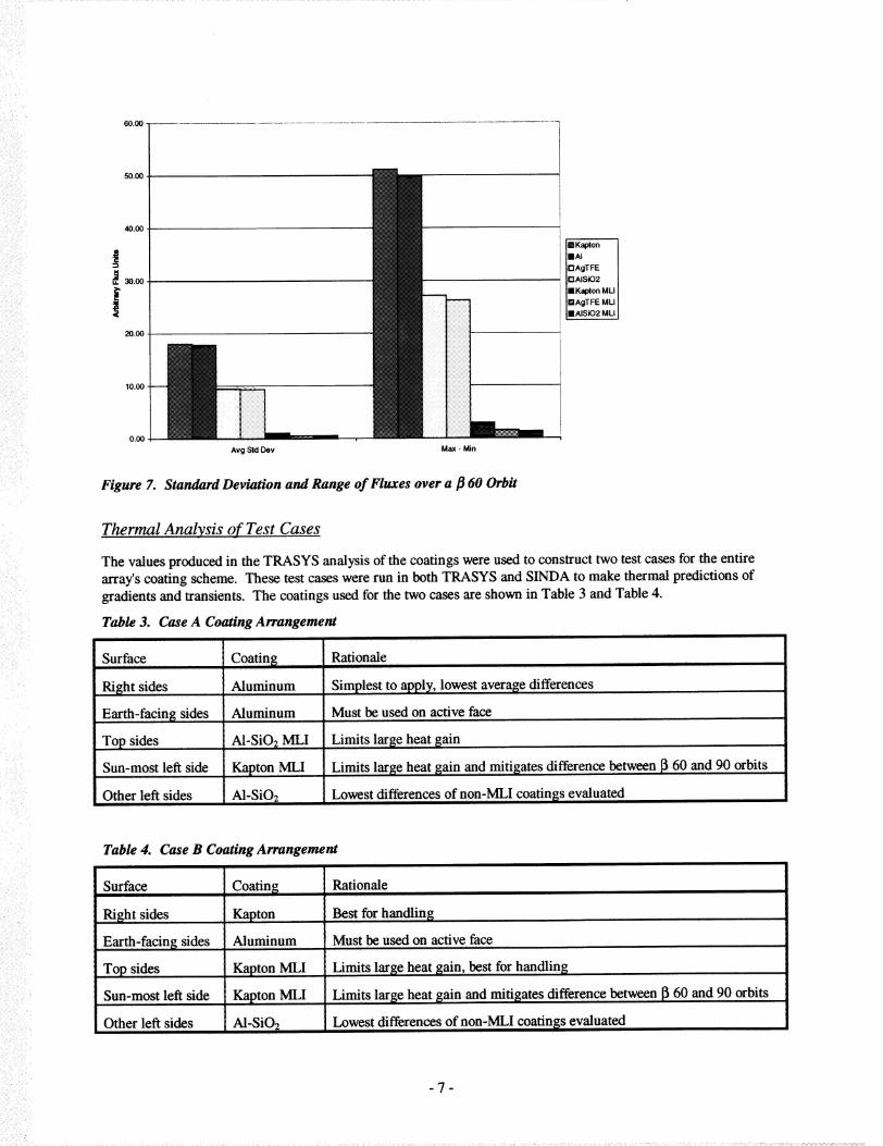
Figure 7. Standard Deviation and Range of Fluxes over a [3 60 Orbit ..................................................................... 7

Figure 8. Comparison of Cases A and B ................................................................................................................ 8

Figure 9. Maximum Waveguide Gradients for Orbit Average Cases ...................................................................... 9

Figure 10. Maximum Waveguide Gradients for Cases A and B (Transient Analysis) ........................................... 10

Figure 11. Waveguide Transients for Cases A and B ........................................................................................... 10

Figure 12. Gradients for Thermal Conductivity (k) Comparison .......................................................................... 11

Figure 13. Comparison of Performance for k Variation ....................................................................................... 11

Figure 14. Waveguide Transients for k Comparison ............................................................................................ 12

Figure 15. TRASYS Model of Array ................................................................................................................... 12

Figure 16. Orbit Average Case ([3 90) for A1 7075 ............................................................................................... 14

Figure 17. Orbit Average Case (_ 90) for T50/934 .............................................................................................. 14

Figure 18. Orbit Average Case ([3 90) for XN70 .................................................................................................. 15

Figure 19. Transient Plot for XN70 -- _ 90 Orbit ................................................................................................ 15

Figure 20. Transient Plot for XN70 -- [3 60 Orbit ................................................................................................ 16

Figure 21. Thermal Gradient for XN70 in [3 60 Transient Case (t = 0.8 hours) .................................................... 16

Figure 22. Simplified Two-waveguide Finite Element Model .............................................................................. 17

Figure 23. Detailed View of Two-waveguide Finite Element Model with Aperture Slots ...................................... 18

Figure 24. Deflections (inches) in Y-direction without Aperture Slots (A1 7075) ................................................. 18

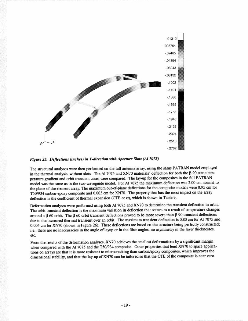
Figure 25. Deflections (inches) in Y-direction with Aperture Slots (A1 7075) ...................................................... 19

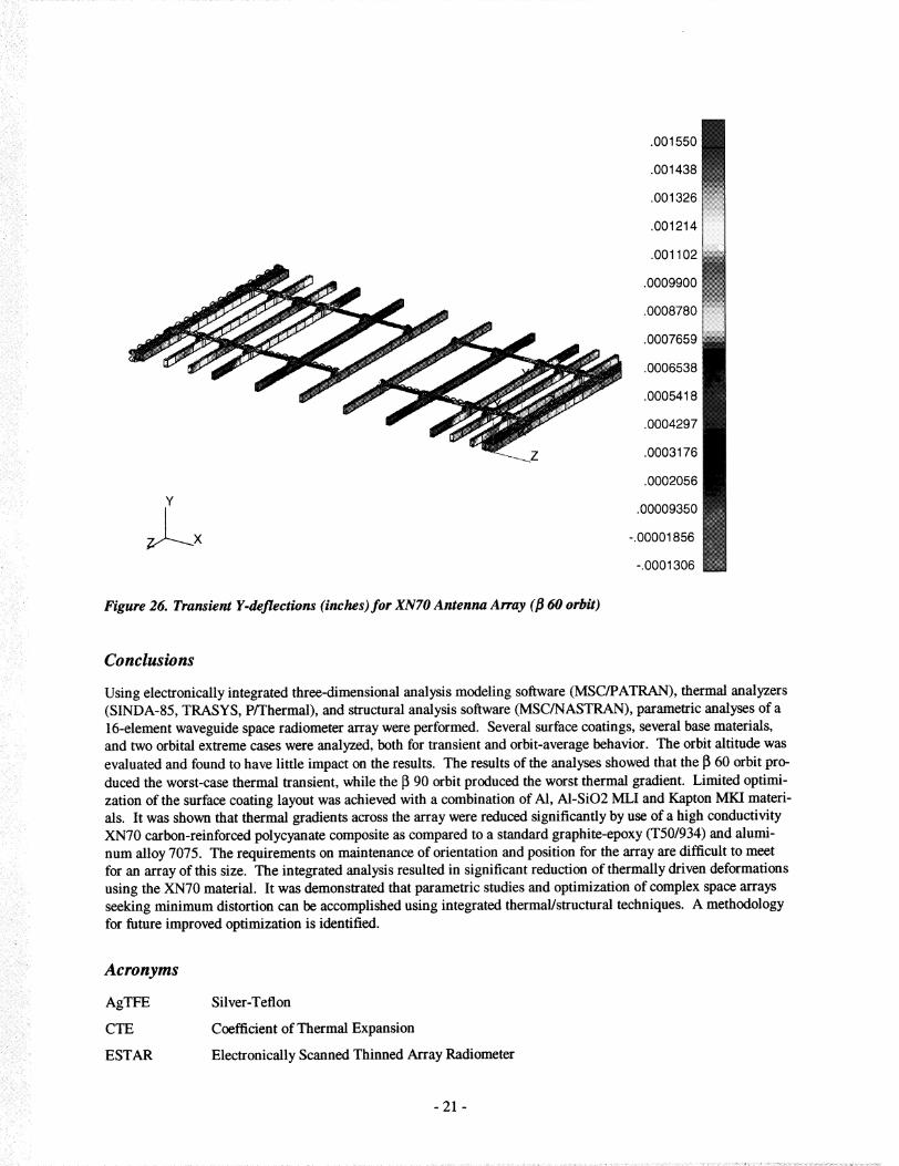
Figure 26. Transient Y-deflections (inches) for XN70 Antenna Array ([3 60 orbit) ............................................... 21

Tables

Table 1. Optical Properties Used for Thermal Coatings ......................................................................................... 3

Table 2. Example TRASYS Test Case Results ....................................................................................................... 4

Table 3. Case A Coating Arrangement .................................................................................................................. 7

Table 4. Case B Coating Arrangement .................................................................................................................. 7

Table 5. Case A and B Orbit-Average Results ....................................................................................................... 8

Table 6. Example Transient Test Case (Case A, 1_60 orbit, 420 km altitude -- all values in °C) ............................ 9Table 7. Case A and B Performance Measures ..................................................................................................... 10

Table 8. Total Array Thermal Gradient for 3 Materials ....................................................................................... 13

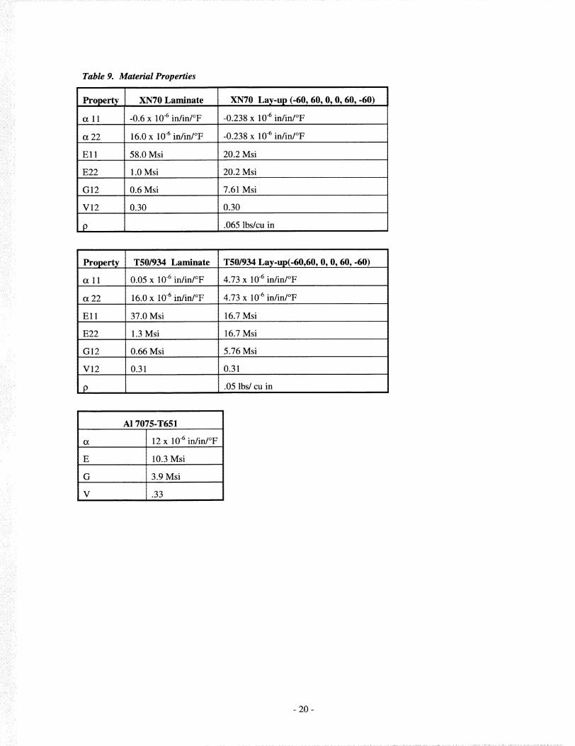
Table 9. Material Properties ................................................................................................................................ 20

1

Abstract

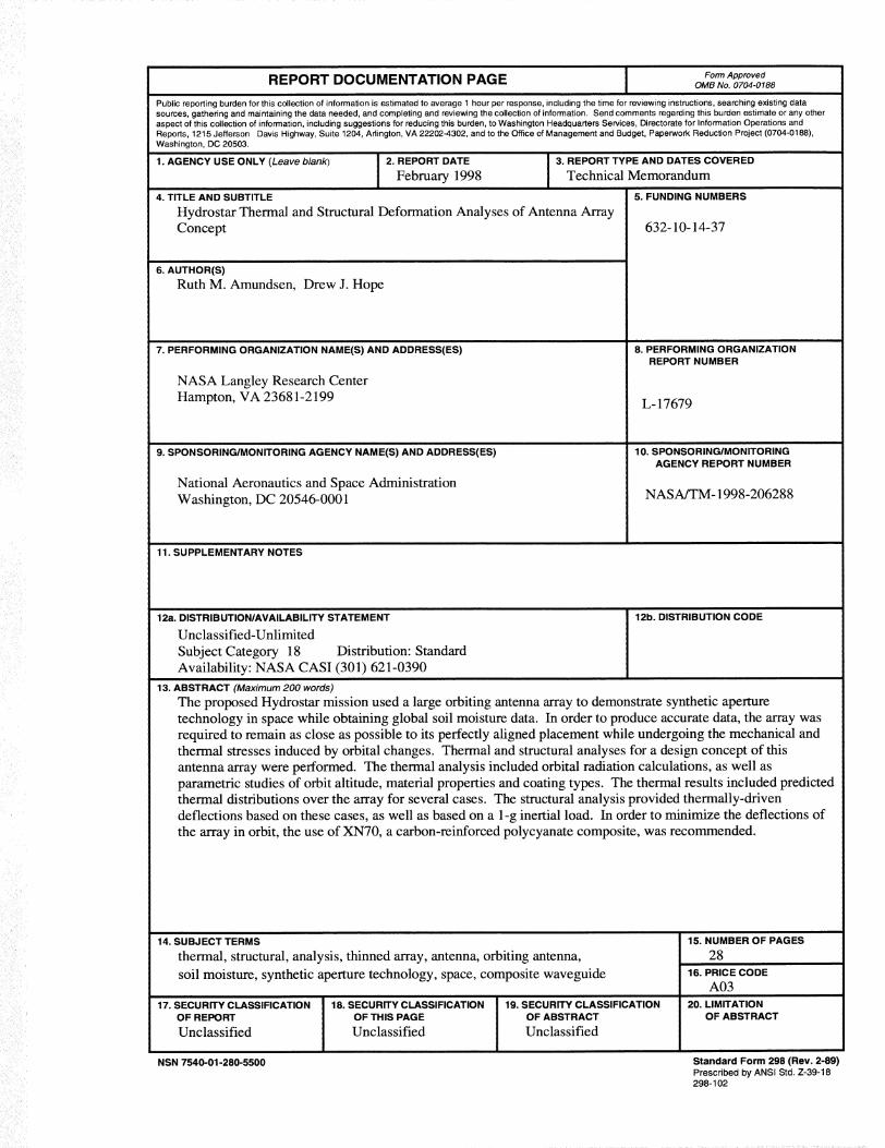
The proposed Hydrostar mission used a large orbiting antenna array to demonstrate synthetic aperture technology

in space while obtaining global soil moisture data. In order to produce accurate data, the array was required to

remain as close as possible to its perfectly aligned placement while undergoing the mechanical and thermal

stresses induced by orbital changes. Thermal and structural analyses for a design concept of this antenna array

were performed. The thermal analysis included orbital radiation calculations, as well as parametric studies of orbit

altitude, material properties and coating types. The thermal results included predicted thermal distributions over

the array for several cases. The structural analysis provided thermally-driven deflections based on these cases, as

well as based on a 1-g inertial load. In order to minimize the deflections of the array in orbit, the use of XN70, a

carbon-reinforced polycyanate composite, was recommended.

Introduction

There have recently been several programs at NASA Langley Research Center involving design of large orbiting

antenna arrays for synthetic aperture radiometer measurements 1'2'3. ICESTAR was a proposed microwave radi-

ometer array to measure and track large-scale movements of ice ridges and leads over the North Pole regions to

facilitate sailing and shipping via a polar sea route 4. ESTAR was a proposed array to measure soil moisture from a

satellite platform 5. Some detailed thermal analysis was performed for ESTAR to evaluate the stability for

waveguide-mounted electronics 6. Hydrostar was a proposal for a joint mission by NASA Goddard Space Flight

Center and NASA Langley Research Center (as well as several other industrial collaborators). The Hydrostar mis-

sion objective was to demonstrate synthetic aperture technology in space while obtaining global soil moisture data 7.

One of the most challenging requirements on any of these arrays is that, to take accurate measurements, the array

must remain planar and well aligned while in orbit. This means that the separate waveguide elements must not

move or twist in relation to each other, and must also accurately retain their own original shape. There are two

types of requirements on the array stability. The first is that the array elements must be within some tolerance of

their ground-test positions when the array is initially deployed on-orbit. This is the initial deployment accuracy,

and the stringency on this requirement will depend on how well an initial on-orbit calibration 8'9 canbe performed.

The second type of requirement is on changes over an orbit, i.e., the orbital stability. The level of this requirement

will depend on whether calibrations can be done as frequently as once per orbit, and how much motion of the

waveguides can be tolerated and still carry out a successful calibration. For each class of stability requirement,

there will be six tolerance values -- one for each axis of translation and rotation. In addition, there may be

different tolerances on the motion of waveguides close to each other (e.g., tolerance on relative motion of first to

second waveguide) as opposed to waveguides that are far apart (e.g., first to last waveguide). All of these position

requirements will also be affected by the required accuracy and measurement resolution of the array. Another

potential requirement is that the array should remain relatively stable in temperature over the course of a year, as

well as over the course of an orbit. For the Hydrostar program, these requirements were not yet completely

specified at the time the thermal and structural analyses were performed. However, an order-of-magnitude number

of less than one centimeter of motion was defined as a starting point. The angular rotation tolerance was about 1

degree. More specific values were roughly set at the following: initial deployment spacing accuracy of 2 mm for

closest waveguides and 2 cm for most distant waveguides; orbital stability out-of-plane 1 cm and in-plane 5 mm/m.

These requirements would need to be completely determined before final analysis of a flight design antenna was

performed.

The baseline Hydrostar array consisted of 16 waveguide elements that were each 5.8 meters in length. The full

array deployed to a width of 9.8 m. Each array element, or waveguide, had a hollow rectangular cross-section of

16.9 cm x 8.6 cm. The wavelength 0_) used was 10.7 cm. The large dimensions of the overall array, and the rela-

tively small sizes of the waveguide walls, led to interesting challenges in modeling, as discussed below.

Both thermal and structural analyses were performed on the baseline Hydrostar array concept to define the maxi-

mum deformations predicted as a result of thermal gradients. An orbital analysis was performed to define the or-

bital fluxes on the surfaces of the array elements and support truss. Several parametric analyses were performed in

an attempt to determine the optimum surface coating for thermal objectives. A thermal analysis was performed

using the orbital fluxes, to define the thermal gradient over the entire array and to predict the thermal transient

overthecourseofanorbit.Finally,severalstructuralanalyseswereperformedusingthepredictedtemperaturedistributions,topredicton-orbitdeflectionsduetothethermalvariations.Severaldifferentmaterialswereevalu-atedfortheirperformanceboththermallyandstructurally.

Orbital Analysis

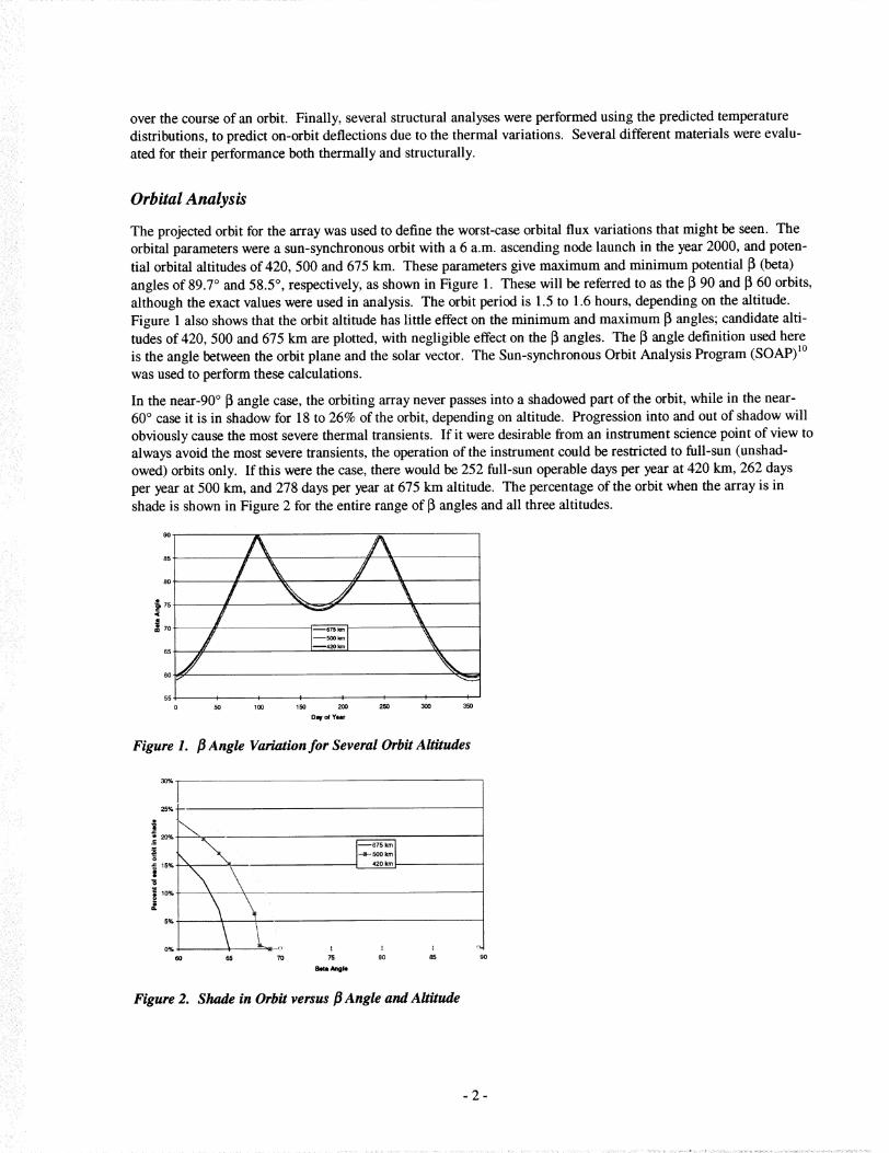
The projected orbit for the array was used to define the worst-case orbital flux variations that might be seen. The

orbital parameters were a sun-synchronous orbit with a 6 a.m. ascending node launch in the year 2000, and poten-

tial orbital altitudes of 420, 500 and 675 km. These parameters give maximum and minimum potential [_ (beta)

angles of 89.7 ° and 58.5 °, respectively, as shown in Figure 1. These will be referred to as the [3 90 and [_ 60 orbits,

although the exact values were used in analysis. The orbit period is 1.5 to 1.6 hours, depending on the altitude.

Figure 1 also shows that the orbit altitude has little effect on the minimum and maximum 13angles; candidate alti-

tudes of 420, 500 and 675 km are plotted, with negligible effect on the [_ angles. The 13angle definition used here

is the angle between the orbit plane and the solar vector. The Sun-synchronous Orbit Analysis Program (SOAP) 1°

was used to perform these calculations.

In the near-90 ° [3 angle case, the orbiting array never passes into a shadowed part of the orbit, while in the near-60 ° case it is in shadow for 18 to 26% of the orbit, depending on altitude. Progression into and out of shadow will

obviously cause the most severe thermal transients. If it were desirable from an instrument science point of view toalways avoid the most severe transients, the operation of the instrument could be restricted to full-sun (unshad-

owed) orbits only. If this were the case, there would be 252 full-sun operable days per year at 420 km, 262 days

per year at 500 km, and 278 days per year at 675 km altitude. The percentage of the orbit when the array is in

shade is shown in Figure 2 for the entire range of 13angles and all three altitudes.

A85

r_7s

1--42o k_ !65

60

55 , , , , , I

0 5o 100 150 200 250 300

Day of Year

i

35O

Figure 1. /3 Angle Variation for Several Orbit Altitudes

J \m20%

o

15%

10%-

5%

0%

6O 65 70

I--_-s00_. II 420 km

80 85

Beta Angle

9O

Figure 2. Shade in Orbit versus 1_Angle and Altitude

ParametricEvaluations

Radiative Analysis of Coatings

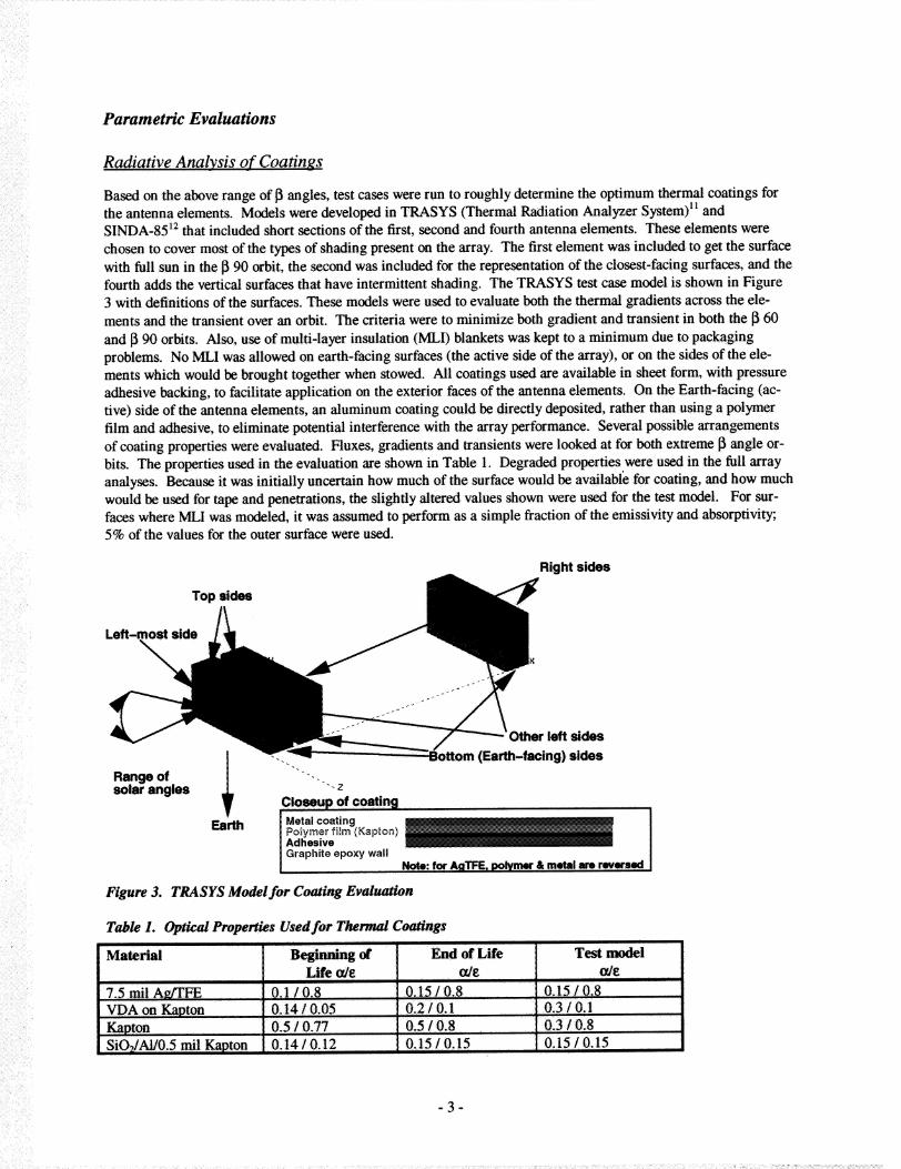
Based on the above range of 13angles, test cases were run to roughly determine the optimum thermal coatings forthe antenna elements. M_ls were developed in T_SYS (Thermal Radiation Analyzer Sy_m)11 andSINDA-85 _2 that included short sections of the first, second and fourth antenna elements. These elements were

chosen to cover most of the types of shading present on the array. The first element was included to get the surface

with full sun in the 13:90 orbit, the second was included for the representation of the closest,facing surfaces, and thefourth adds the vertical surfaces that have intermittent shading. The TRASYS test case model is shown in Figure

3 with definitions of the surfaces. These models were u_ to evaluate both the thermal gradients across the ele-

ments and the transient over an orbit. The criteria were to minimize both gradient and transient in both the [3 60

and 1390 orbits. Also,, use of multi-layer insulation (_I) blankets was kept to a minimum due to packaging

problems:. No _I w_ allowed on earth-facing surfaces (the active side of the array), or on the sides of the ele-

ments which would be brought together when stowed. All coatings used are available in sh_t form, with pressure

adhesive backing, to facilitate application on the exterior faces of the antenna elements. On the Earth-facing (ac-

tive) side of the antenna elements, an aluminum coating could be directly deposited, rather than using a polymer

film and adhesive, to eli_nate potential interference with the array performance. Several possible _angements

of coating properties were evaluated. Fluxes, gradien_ and transients were looked at for both extreme 13_gle or-

bits. The properties used in the evaluation are shown in Table 1. Degraded properties were used in the fidl arrayanalyses. Because it was initially uncertain how much of the surface would be available for coating, and how much

would be used for tape and penetrations, the slightly altered values shown were used for the test model. For sur-

faces where MLI was modeled, it was assumed to perform as a simple ft'action of the emissivity and absorptivity;5% of the values for the outer surface were used.

Top sides

Right sides

Left-most side

Range ofsolar angles 1

Earth

Other left sides

-.. (Earth-_ing) sides

Closeup of coating

Meta|coating ...............................Polymerfilm (Kapton) _AdhesiveGraphiteepoxywall

Note:for Ag_ polymer&-metalarereversed.

Figure 3. TRASYS Model for Coating Evalm_'on

Table 1. Op_al Prop--s Used for T_rmal Coaangs[ i i i

Material

VD A on Kapton

Ka_on

SiO2/_0.5 mil Kapton

Beg_ng ofLife _

' II

0.1/0.801.14 / 0.05

0.5 I0.77

0.1.4/0.12 ,

' End ofLife Test _!

:: " r i i

O.I5/0.8 O.15/0.80.210.1 0.3 / 0.1

0.5 I0.8 ..... 0.3 10.80..15 t 0..15 0.15 / 0.15

.... i i "

The TRASYS model of this test case used only one surface per side of each waveguide. This produced accurate

TRASYS radiative results. However, in the SINDA-85 and P/Thermal 13models, this assumption led to some inac-

curacy in the predicted gradients. PATRAN P/Thermal models were only developed for the full array, and not for

the test case. In the full array models, there was still only one node or surface defined across the width of each side

of the waveguide, although there were many nodes along the length. The reason the models were kept at such a

relatively coarse mesh was to stay within the TRASYS overall limit on number of surfaces. For the SINDA mod-

els, there will not be much error in the gradients, since the lumped node is in the center of each side, and thus con-

ductance and TRASYS heat input will be defined from the center of each side, and will be numerically correct.

However, in the P/Thermal models, with the version of MSC/PATRAN used in this analysis (5.0), the nodes are

defined as in a finite element model, at the corners of each element. Thus, the heat fluxes and radiation to space

are apportioned to the corners, and some of the driving forces for the gradients are lost. Basic conclusions and

trends can still be drawn from this analysis, although a more detailed model should be done if this analysis is to be

used for flight hardware design. A more detailed model can be done using this analysis method by applying the

TRASYS fluxes from a coarse mesh model to a more detailed finite element model, i.e., each TRASYS flux is ap-

plied to several finite elements. However, because of the dimensions and number of the waveguides, more finely

dividing the mesh quickly drives the model to an unwieldy size.

Seven different optical coatings were evaluated; the seven coatings consisted of the four coatings in Table 1, and

each one as the outer layer of an MLI blanket (except for the vapor deposited aluminum). First, a TRASYS model

was run for each as the sole coating on all surfaces of the test model. For each case, the heat flux input from solar,

Earth albedo and Earth IR was summed on each surface. Then the amount of heat lost to space via radiation was

subtracted, leaving the effective net power gained or lost by that surface, as an orbit average. This was done for

both 60 and 90 ° _ angle orbits. An example of this calculation is shown in Table 2.

Table 2. Example TRASYS Test Case Results

Surface Prop-

erty, tz/8Orbit

Surface

WG1 right

WG1 base

WG 1 left

WG1 top

WG2 rightWG2 base

WG2 left

WG2 top

WG3 right

WG3 base

WG3 left

WG3 top

Q input

(Btu/hr)

6.70

59.10

58.46

10.26

18.48

59.10

8.08

10.26

17.09

59.10

58.07

10.26

.15/.8

beta 60

Rk to

space

Q output

(Btu/hr)

Difference

(Btu/hr)

0.07 7.03 -0.3

0.25 24.94 34.2

0.50 49.13 9.3

0.25 24.94 -14.7

0.49 48.22 -29.7

0.25 24.94 34.2

0.07 7.03 1.1

0.25 24.94 -14.7

0.50 49.13 -32.0

0.25 24.94 34.2

0.49 48.22 9.9

0.25 24.94 -14.7

Q input

(Btu/hr)

2.25

54.00

81.24

0.04

16.52

54.00

2.26

0.04

16.43

54.00

16.96

0.04

Rk to

space

.15/.8

beta 90

Q output

(Btu/hr)

Difference

(Btu/hr)

0.07 7.03 -4.8

0.25 24.94 29.1

0.50 49.13 32.1

0.25 24.94 -24.9

0.49 48.22 -31.7

0.25 24.94 29.1

0.07 7.03 -4.8

0.25 24.94 -24.9

0.50 49.13 -32.7

0.25 24.94 29.1

0.49 48.22 -31.3

0.25 24.94 -24.9

In order to calculate the heat lost to space, a temperature for the entire array had to be assumed. This will be de-

pendent not only on the optical properties on the surfaces, but also on electronics self-heating, spacecraft tempera-

ture and operational scenarios. In fact, the decision might be made to use resistance heating to hold the array at a

warmer temperature than it would normally attain. Since the array temperature could not be known at this point,

the cases were run for several different assumed array temperatures to discern the impact that variable would have.

Four different array temperature cases were run for each surface type and each orbit case: -70 °, -50 °, -20 ° and 0°C.

Only two of these temperature cases are shown, since all led to roughly the same results.

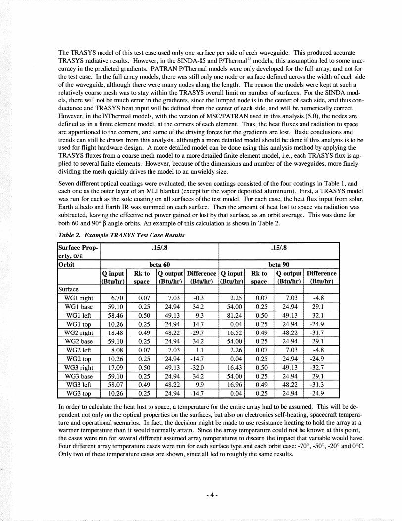
Theeffectiveheatgainedor lost by the surface (Qnet = Qin - Qou0 was averaged for the [3 60 and [3 90 orbits as a

root-mean-square [Qavg- (Qin 2 + Qout2)l/2], since some net heating values were negative. This averaging allowed

selection of a coating that is optimized over the entire range of 13angles. The number of effective surfaces was

reduced from twelve to five, by averaging together similar surfaces that would probably receive the same coating

(e.g., all top surfaces averaged). This was done since the results for same-facing surfaces were similar, and the use

of similar coatings on equivalent waveguide surfaces facilitates manufacturing and assembly. The only exception

was that the left-most surface was kept separate, as it is the only left.hand surface to receive full sun, and conse-

quently might be the only one to receive a different coating. Thus the averages are: all right sides (away from the

sun), all Earth-facing sides (bases), all tops, the sun-most (outer-most) left side, and all other left sides.

The objectives for the optimum coatings are as follows:

(1) The differences in net heating between surfaces should be as small as possible, in order to minimize the ther-

mal force driving the waveguide gradients. In other words, a coating should be selected for each surface that

results in the net heating values for all surfaces being as close to equal as possible.

(2) The change in heating rates over the course of an orbit should be as small as possible, to optimize the orbital

temperature stability.

(3) The difference in net heating between the _ 60 and _ 90 orbits should be as small as possible, to minimize the

temperature change over the year.,

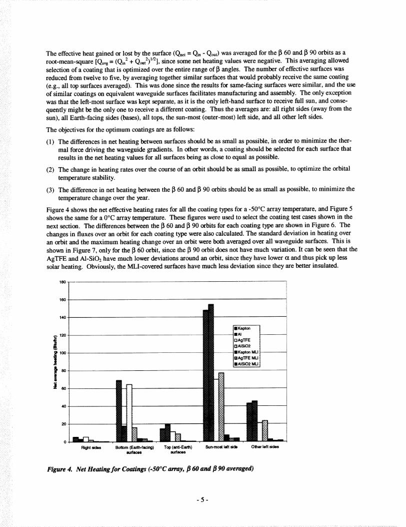
Figure 4 shows the net effective heating rates for all the coating types for a -50°C array temperature, and Figure 5shows the same for a 0°C arr_ temperature. These figures were used to select the coating test cases shown in the

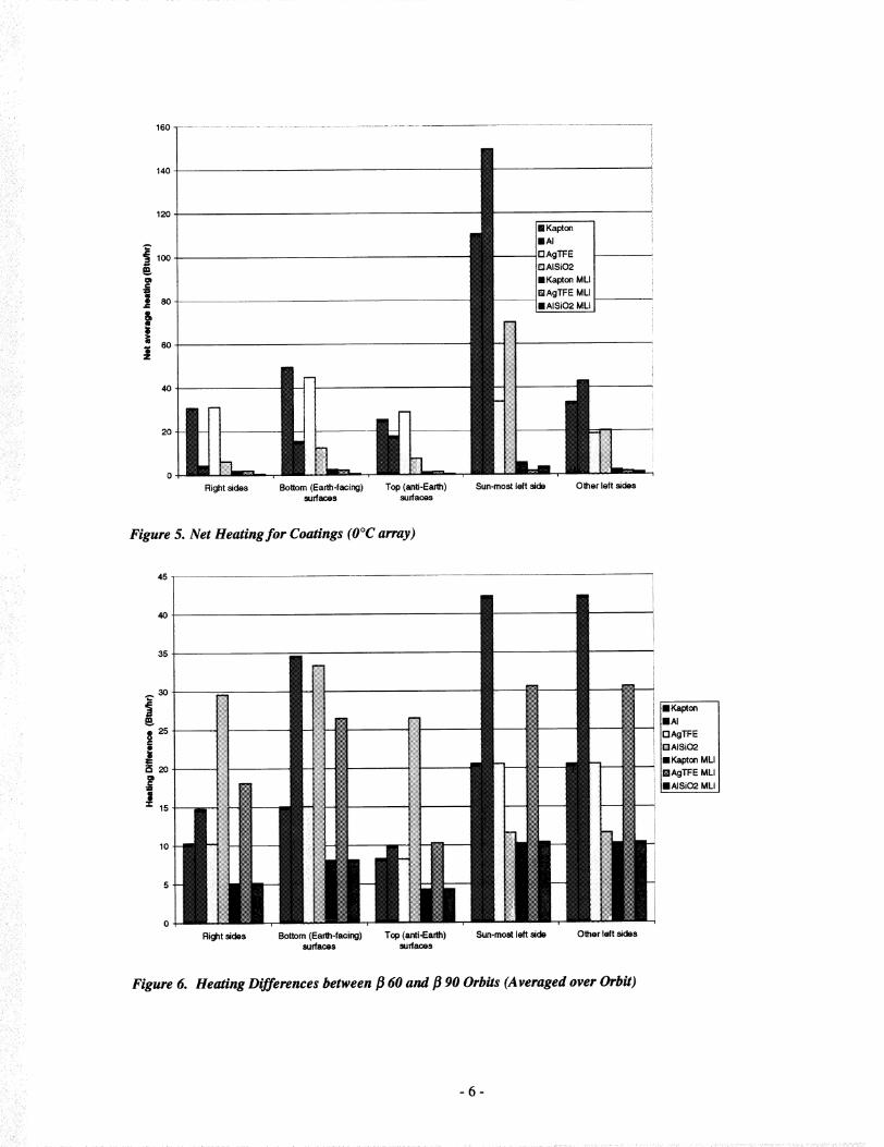
next section. The differences be_een the 1360 and 1390 orbits for each coating type are shown in Figure 6. The

changes in fluxes over an orbit for each coating type were also calculated. The standard deviation in heating over

an orbit and the maximum heating change over an orbit were both averaged over all waveguide surfaces. This is

shown in Figure 7, only for the 1360 orbit, since the 1390 orbit does not have much variation. It can be seen that the

AgTFE and A1-SiO2 have much lower deviations around an orbit, since they have lower (x and thus pick up less

solar heating. Obviously, the MLI-covered surfaces have much less deviation since they are better insulated.

180]160

140

,_ 120

||I 8o

40

Right sides

I

I m KalXonIIAI

[:]AgTFEBAISi02

lKa_on MLI

m BAg_E billIAiS*02MU

l _i))iJ

m ¸ ,

m,0 II

.........

Bottom (Eaah4acing) Top (ardi,Earlh) Sun-most left side Olher left-sidessurfaces surfaces

Figure 4. Net Heating for Co_ngs (-50°C array, fl 60 and fl 90 averaged)

i:̧ i_ii:_̧

/i,_I'_::_

/

160

140

120

1:00

el¢=

|,j= 8o

&I1

il6O

4O

2o/_ II .n0 ......

Right sides Bottom (Earth.facing) Top (_ti.Earth)surfaces surfaces

d EKapton[]At

G AgUE

I NAISiO2IIKapton MLI

[] AgTFE MLI

HI AISi02 MLI

/ iiiiiiiiii;i m

/_......il_l _iiiii._ I[I__'.......

_n-most left side Other left sides

Figure 5. Net Heating for Coatings (O°C array)

45

40

l"AI I

25 .... I ; i lQAgTFEJ i " !="_'_MLI

iiAISiO2 MLI

10 !

5

.................. . ,,,

0 .............. .........

Right sides Bottom (Ea_.facing) Top (anti.Ea_) Sun-most left side Other left sidessurfaces surfaces

Figure 6. He_ng Differences between ]3 60 and _] 90 Orbits(Averaged over Orbit)

ii!:ii/!/

!!i!ii_i,iiiii_i!:_

i:ii!!iiiiii_iiiiiiii:i

60.00

50.00

40.00

t

30.00

20.00

10.00

0.00

Avg StdDev Max - Min

Figure 7. Standard Deviation and Range of Fluxes over a [360 Orbit

!eKam°n II_U

iOAgTFE t

p,,s_2 Ii-Ka.o._UIleAgTFEMLIIt,,^ts_2MuI

Thermal Analysis of Test Cases

The values produced in the TRASYS analysis of the coatings were used to construct two test cases for the entire

array,s coating scheme. _ese test cases were run in _th TRASYS and SINDA to make thermal predictions of

gradients and transients. The coatings used for the two cases are shown in Table •3 and Table 4.

Table 3. Case A Coating Arrangement...........

Surface Coatin[[ Rationale-- .... .... ............ .... i " ....' " "

Right sides , Aluminum ..... Simplest tO apply, lowest avera[e differences ....

Earth-facin[_ sides ._luminum Must be used on active face............ " .... i .............

Top sides A1-SiO2 _I Limits lar[e heat _ain

Sun-most left side

Other left sides

i Kapton MLI i Limits larse heat _ain and _ti_ates difference between _ 60and 90 orbits ,

Al-Si02 Lowest _fferences of non-MLl coatings evaluated

Table 4. Case B Coating Arrangement

Surface . Coatin_ Rationale ,.........

_ght sides n'Kapt0n . Best for handin[[

E_thTfa_dn[_ sides n Aluminum Must be used on activeface

Top sides Kapton MLI . Limits larse heat [[ain, best for handlin[_

Sun-most le_ side

Other left sides

Kapton MLI, Li_ts large heat gain and mifif[ates difference between [$ 60 and 90 orbits

Al-SiO2 Lowest differences of non-_I coatings evaluated

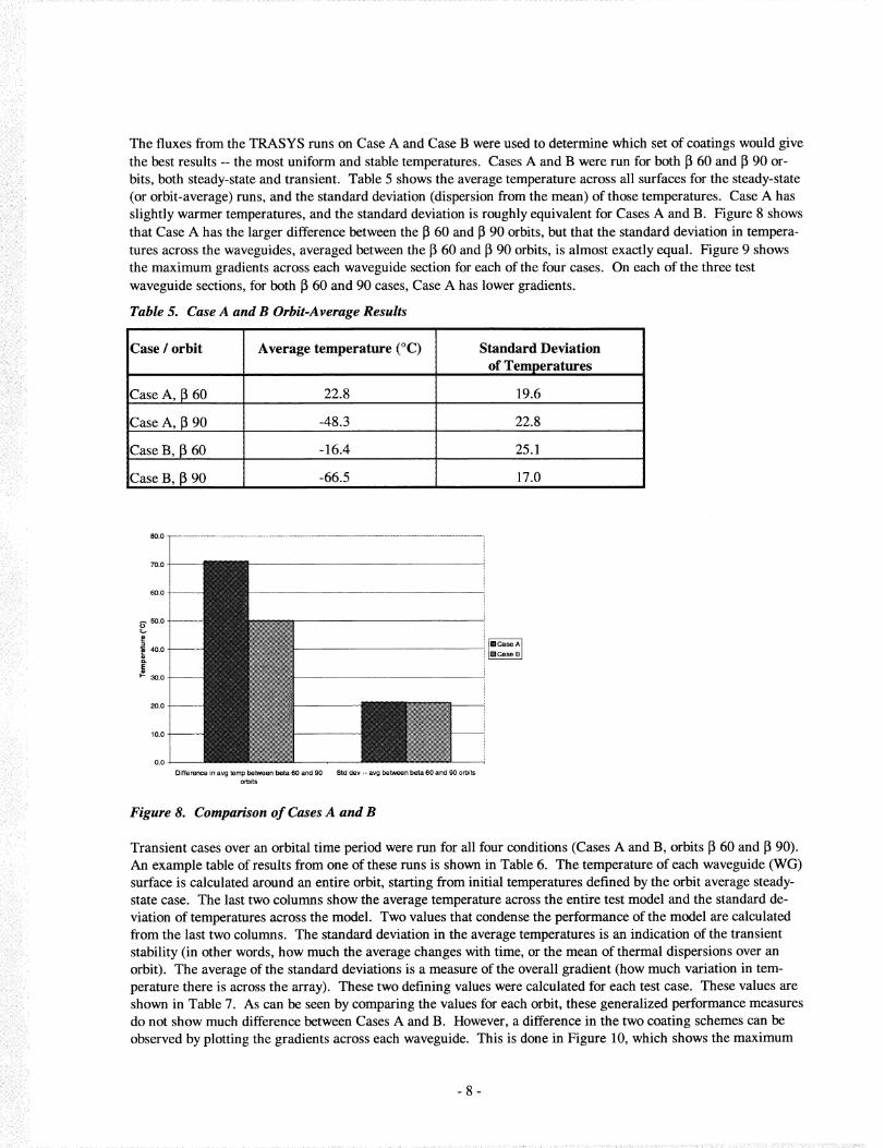
ThefluxesfromtheTRASYSrunson Case A and Case B were used to determine which set of coatings would give

the best results -- the most uniform and stable temperatures. Cases A and B were run for both 1360 and 1390 or-

bits, both steady-state and transient. Table 5 shows the average temperature across all surfaces for the steady-state

(or orbit-average) runs, and the standard deviation (dispersion from the mean) of those temperatures. Case A has

slightly warmer temperatures, and the standard deviation is roughly equivalent for Cases A and B. Figure 8 shows

that Case A has the larger difference between the 1360 and 1390 orbits, but that the standard deviation in tempera-

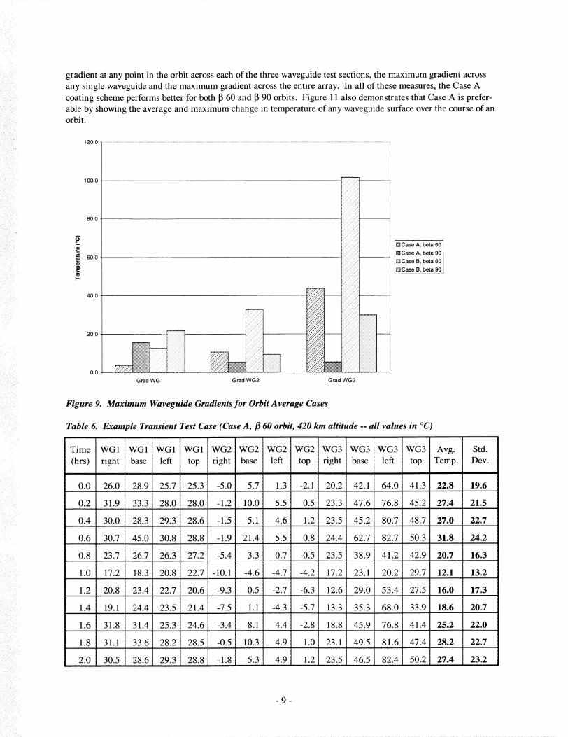
tures across the waveguides, averaged between the 1360 and 1390 orbits, is almost exactly equal. Figure 9 shows

the maximum gradients across each waveguide section for each of the four cases. On each of the three test

waveguide sections, for both 1360 and 90 cases, Case A has lower gradients.

Table 5. Case A and B Orbit-Average Results

i!ii!!!!iiiiii!!!!:iii_!_i_i_,il/

_i!! ii

Case / orbit

Case A, 1360

Case A, 1390

Case B, 1360

Case B, 1390

Average temperature (°C)

22.8

Standard Deviation

of Temperatures

19.6

22.8

25.1

17.0

70.0

60.0

6" 5o.oe.,o

40.0

I- 30.0

20.0

10.0

0.0

Difference in avg temp between beta 60 and 90 Std dev -- avg between beta 60 and 90 orbits

orbits

Figure 8. Comparison of Cases A and B

Transient cases over an orbital time period were run for all four conditions (Cases A and B, orbits 1360 and 1390).

An example table of results from one of these runs is shown in Table 6. The temperature of each waveguide (WG)

surface is calculated around an entire orbit, starting from initial temperatures defined by the orbit average steady-

state case. The last two columns show the average temperature across the entire test model and the standard de-

viation of temperatures across the model. Two values that condense the performance of the model are calculated

from the last two columns. The standard deviation in the average temperatures is an indication of the transient

stability (in other words, how much the average changes with time, or the mean of thermal dispersions over an

orbit). The average of the standard deviations is a measure of the overall gradient (how much variation in tem-

perature there is across the array). These two defining values were calculated for each test case. These values are

shown in Table 7. As can be seen by comparing the values for each orbit, these generalized performance measures

do not show much difference between Cases A and B. However, a difference in the two coating schemes can be

observed by plotting the gradients across each waveguide. This is done in Figure 10, which shows the maximum

ii i;, ::i

_ i i!_ i

il!iq_:!illi!i_!__i_i_!_iill_ii_,_:_.il

i_!!!_iiii!i!:iiiiii!iii_:iii_::_

gradient at any point in the orbit across each of the three waveguide test sections:, the maximum gradient across

any single waveguide and the maximum gradient across the entire array. In all of these measures, the Case A

coating scheme performs better for both 1360 and 1390 orbits. Figure 11 also demonstrates that Case A is prefer-

able by showing the average and maximum change in temperature of any waveguide surface over the course of anorbit.

i!ii?L

120.0 ......................................................................................................................................................................................................................................................................

100.0

80.0

t_o

60.0

40.0

20.0

0.0

Grad WG1 Grad WG2

[[]Case A, beta60

_J : :::::'":::"" I []....... ,. Case A, beta 90i_ Case B, beta 60

iN Case B, beta 90

G rad WG3

Figure 9. Maximum Waveguide Gradients for Orbit Average Cases

Table 6. Example Transient Test Case (Case A, fl 60 orbit, 420 km altitude -- all values in °C)

Time WG1

(hrs) right

WG1 WG1 WG1 WG2 WG2 WG2 WG2 WG3 WG3 WG3 WG3

base left top right base left top right base left top

0.0 26.0 28.9 25.7 25.3 -5.0 5.7 1.3 -2.1 20.2 42.1 64.0 41.3

0.2 31.9 33.3 28.0 28.0 -1.2 10.0 5.5 0.5 23.3 47.6 76.8 45.2

Avg.

Temp.

22.8

27.4

Std.

Dev.

19.6

21.5

0.4 30.0 28.3 29.3 28.6 -1.5 5.1 4.6 1.2 23.5 45.2 80.7 48.7 27.0 22.7

0.6 30.7 45.0 30.8 28.8 -1.9 21.4 5.5 0.8 24.4 62.7 82.7 50.3 31.8 24.2

20.70.8 23.7 26.7 26.3 27.2 -5.4 3.3 0.7 -0.5 23.5 38.9 41.2 42.9

1.0 17.2 18.3 20.8 22.7 -10.1 -4.6 -4.7 -4.2 17.2 23.1 20.2 29.7 12.1

16.3

13.2

1.2 20.8 23.4 22.7 20.6 -9.3 0.5 -2.7 -6.3 12.6 29.0 53.4 27.5 16.0 17.3

18.61.4 19.1 24.4 23.5 21.4 -7.5 1.1 -4.3 -5.7 13.3 35.3 68.0 33.9 20.7

1.6 31.8 31.4 25.3 24.6 -3.4 8.1 4.4 -2.8 18.8 45.9 76.8 41.4 25.2 22.0

1.8 31.1 33.6 28.2 28.5 -0.5 10.3 4.9 1.0 23.1 49.5 81.6 47.4 28.2 22.7

2.0 30.5 28.6 29.3 28.8 -1.8 5.3 4.9 1.2 23.5 46.5 82.4 50.2 27.4 23.2

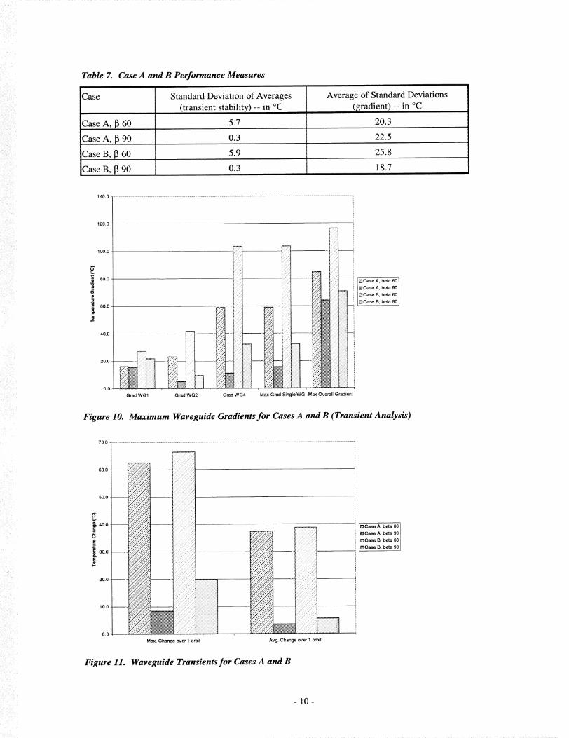
Table 7. Case A and B Performance Measures

i ¸ _ /

ilii_i_i !_i_

:_:::ii;i_: iii!•

Case Standard Deviation of Averages

(transient stability) -- in °C

Case B, 1390

Average of Standard Deviations

(gradient)-- in °C

0.3

Case A, 1360 5.7 20.3

Case A, 1390 0.3 22.5

Case B, [3 60 5.9 25.8

18.7

140.0 ....................................................................................................................................................................................................................... :

120.0

100.0

6"o

.__ 80.0

= 60.0

&E

40.0

20.0 -

0.0

Grad WG1 Grad WG2

E_ Case A, beta 601

[] Case A, beta 90

[]Case B, beta 60

[]Case B, beta 90

Figure 10. Maximum Waveguide Gradients for Cases A and B (Transient Analysis)

70.0 .............................................................................................................................................................................................................................. ,

60.0

50.0

40.0

"_ 30.0

E

20.0

10.0

0.0

•:,. :.:,..,:._,.:.....,._,:,.:_ ._<:.::.:_..!-:

::::--::: ::::\ ::::----................;.f .;:.(¢:: t;./,,:z;._,............

.... ,,,,,.,.y,,,,,.,,..,: ,:.: ,:..:< ,:..:,:::,:,

............

.....iz..z../z..z..//./.://..;z,-:/,,:;.z

/..:;/.(/';/.('5."

._ :.. 5 ¸¸:..¸......I

[iiiiiii!!ii!ii__iiiiii!i!ii:_J........ _..,.:,::?'.i...:::::!....|

_. :.,";,•:..:.-":.I

;; .';;¢..<_;.<;;¢_;,: .... ..:" ::.."..-1

, • __ _ ..................................................................

Avg. Change over 1 orbit

Figure 11. Waveguide Transients for Cases A and B

r'-lCase A, beta 60

[] Case A, beta 90

[]Case B, beta 60

[] Case B, beta 90

.........il

L i_iI,_:_i

!_i_:_iil,_ _iI

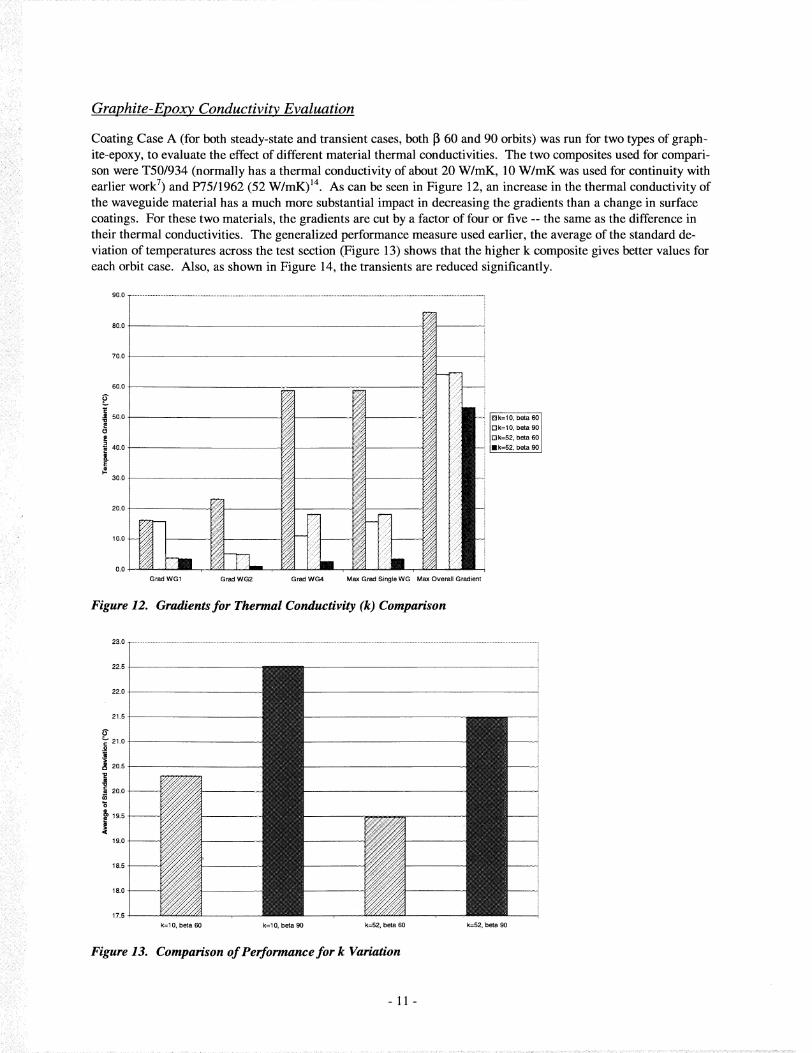
Graphite-Epoxy Conductivity Evaluation

Coating Case A (for both steady-state and transient cases, both [3 60 and 90 orbits) was run for two types of graph-

ite-epoxy, to evaluate the effect of different material thermal conductivities. The two composites used for compari-

son were T50/934 (normally has a thermal conductivity of about 20 W/mK, 10 W/mK was used for continuity with

earlier work 7) and P75/1962 (52 W/mK) 14. As can be seen in Figure 12, an increase in the thermal conductivity of

the waveguide material has a much more substantial impact in decreasing the gradients than a change in surface

coatings. For these two materials, the gradients are cut by a factor of four or five -- the same as the difference in

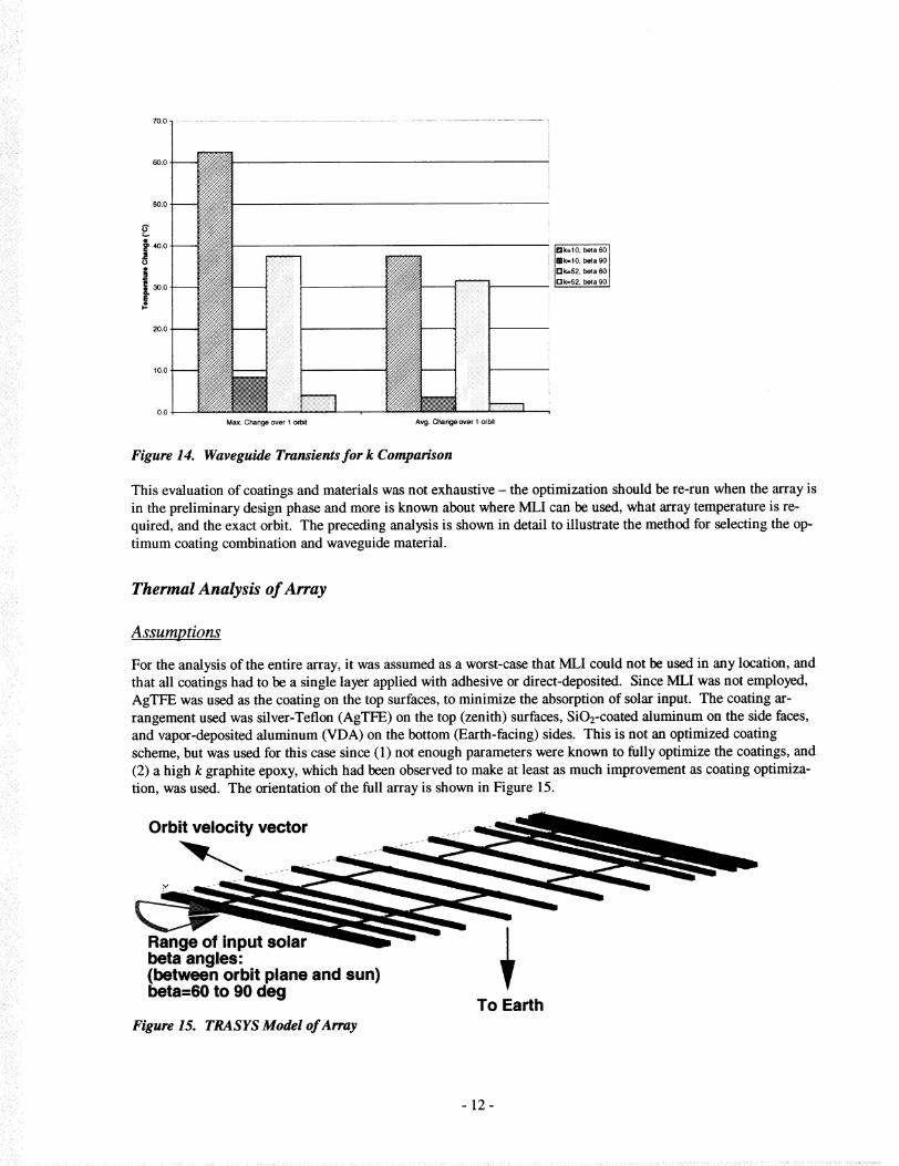
their thermal conductivities. The generalized performance measure used earlier, the average of the standard de-

viation of temperatures across the test section (Figure 13) shows that the higher k composite gives better values for

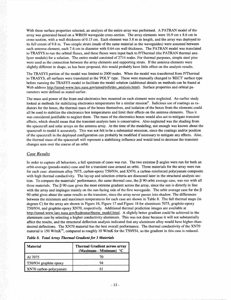
each orbit case. Also, as shown in Figure 14, the transients are reduced significantly.

90.0 ............................................................................................................................................................................................................................. i

iiZ_

80.0 _.:_ _i_:// ..... i

;...:.:;:,,-,,::

7o.o _:_........ i

.... i i::.-..-;:t

.......... _:..>-.x i/. !!;::i

..... _- .........-. :/...s./. , :;"i::!!ifi

..... ..::"i'i.<:

:;:";" iE_!:_ ×_//.. i ili:i!_!i"L" -" ,..........

30.0 ....;:.:.;,:.......... ,2Y"_........ ;"-_'_ i :: ::: :i',:

Grad WG1 Grad WG2 Grad WG4 Max Grad Single WG Max Overall Gradient

60.0.

50.0

40.0

E

Bk=10, beta 60

[] k=l 0, beta 90

[]k=52, beta 60

Ik=52, beta 90

Figure 12. Gradients for Thermal Conductivity (k) Comparison

_!i!_̧;: i _:¸i!¸i¸¸i•̧

?i _:!i_:_I_I:I_i_i

iiii!!_ilI_/%)_

_i:/i__.

ii_:iii_!ii!iiiii!!_!iiill/

; _:ii_iii_iLi,li;__

23.0 ............................................................................................................................................................................................................................................................... .:

22.5

22.0

t"/":/"//""/""//:'/":='..".-L.".*...'.-L.".<-.'/.-'-"

_ j/._./..//...×,.//..:.-.- ._-...-.-...-...-.- ._-.............. ,..,.....,...

.... : ..........:..::..:...:._,....ll....l....i/....l.,iz

.,'..-":,:..'....,:.'-",-...'...-;..,'.-_.'_.::,_!;.................

...........................

18.5 - _ %_)__:_;_)_:_).>

.................:-_:.;::f.f;:-f:;,.;.f.;:f,y.f-f-;................

k=lO, beta 60 k=l O, beta 90

21.5

6"-- 21.0t.-._o"a

20.5

20.0.

"6

19.5

19.0 -

....k=52, beta 60 k=52, beta 90

Figure 13. Comparison of Performance for k Variation

-11-

+_ i

70.0 ..........................................................................................................................................................................

60.0

50.0

v

i} ,o.o2

S

30.0

E

#.

20.0

10.0

0.0 ........

Max. Change over 1 orbit

¸

......................._lill!i!!!_¸:i_!i!_i_i_iii_i:J

Avg. Change over 1 orbit

!

t!!ii_!ii!iii!iiiii!iii!i!i!_i_!iiii!_!!__iii!:i!i:'i:!iiiii'/:!i/i!ii_

!_'_iiiiiiiiiiiiiii!iiiiI

_i!i_i!i_iiiii!i_!!iiiil!..........• ...... _,

= 10, beta 60 I

Irek= 1O, beta 90 I

l.k=52, beta 60 I

lak=52,betaooI

Figure 14. Waveguide Transients for k Comparison

This evaluation of coatings and materials was not exhaustive - the optimization should be re-run when the array is

in the preliminary design phase and more is known about where MLI can be used, what array temperature is re-quired, and the exact orbit. The preceding analysis is shown in detail to illus_ate the method for selecting the op-

timum coating combination and waveguide material.

Thermal Analysis of Array

Assumptions

For the an_ysis of the entire array, it was assumed as a worst-case that _I could not be used in any location, and

that all coatings had to _ a single layer applied with adhesive or direct-deposited. Since _I was not employed,

AgTFE was used as the coating on the top surfaces, to minimize the absorption of solar input. The coating ar-

rangement used was silver-Teflon (AgTFE) on the top (zenith) surfaces, SiO2-coated alu_num on the side faces,

and vapor-deposited aluminum (VDA) on the bottom (Earth-facing) sides. This is not an optimized coatingscheme, but was used for this case since (1) not enough parameters were known to _lly optimize the coatings, and

(2) a high k graphite epoxy, which had been observed to m_e at least as much improvement as coating optimiza-

tion, was used. The orientation of the _11 array is shown in Figure 15.

Orbit velocity vector

Range of input solarbeta angles:(between orbit plane and sun)beta=60 to 90 deg

Figure 15. TRASYS Model of Array

To Earth

i •

ii/_iii_il_i_i_

i_ii _i_i_ii/

i!!iii_

ililii!!!i!iii_!

_ _:i__

i

i/?_iiiiiii!/_!iii'

/!_iiiil!if!i!_ii_i!

With these surface properties selected, an analysis of the entire array was performed. A PATRAN model of the

array was generated based on a WR650 waveguide cross-section. The array elements were 16.9 cm x 8.6 cm in

cross-section, with a wall thickness of 0.15 cm. Each element was 5.8 m in length, and the array was deployed to

its full extent of 9.8 m. Two simple struts (made of the same material as the waveguides) were assumed between

each antenna element, each 7.6 cm in diameter with 0.64-cm wall thickness. The PATRAN model was translated

to TRASYS to run the orbital fluxes, and these fluxes were input back to P/Thermal (the PATRAN thermal ana-

lyzer module) for a solution. The entire model consisted of 2714 nodes. For thermal purposes, simple steel pins

were used as the connection between the array elements and supporting struts. If the antenna elements were

slightly different in shape, as has been proposed, this would probably have little effect on the analysis results.

The TRASYS portion of the model was limited to 2000 nodes. When the model was transferred from P/Thermal

to TRASYS, all surfaces were translated as the 'POLY' type. These were manually changed to 'RECT' surface type

before running the TRASYS model to facilitate the model solution (additional details on methods can be found at

Web address http://amsd-www.larc.nasa.gov/amsd/refs/des analysis.html). Surface properties and orbital pa-rameters were defined as stated earlier.

The mass and power of the front-end electronics box mounted on each element were neglected. An earlier study

looked at methods for stabilizing electronics temperatures for a similar mission6. Judicious use of coatings as ra-

diators for the boxes, the thermal mass of the boxes themselves, and isolation of the boxes from the elements could

all be used to stabilize the electronics box temperatures and limit their effects on the antenna elements. Thus it

was considered justifiable to neglect them. The mass of the electronics boxes would also act to mitigate transient

effects, which should mean that the transient analysis here is conservative. Also neglected was the shading from

the spacecraft and solar arrays on the antenna array. At the time of the modeling, not enough was known about the

spacecraft to model it accurately. This was not felt to be a substantial omission, since the coatings and/or position

of the spacecraft in the deployed configuration can probably be modified if necessary to mitigate any effects. Also,

the thermal mass of the spacecraft will represent a stabilizing influence and would tend to decrease the transient

changes seen over the course of an orbit.

Case Results

In order to capture all behaviors, a full spectrum of cases was run. The two extreme _l angles were run for both an

orbit-average (pseudo-static)case and for a transient case around an orbit. Three materials for the array were run

for each case: aluminum alloy 7075, carbon-epoxy T50/934, and XN70, a carbon-reinforced polycyanate composite

with high thermal conductivity. The lay-up and selection criteria are discussed later in the structural analysis sec-

tion. To compare the materials' performance, the same thermal case, the _ 90 orbit average case, was run with all

three materials. The _l 90 case gives the most extreme gradient across the array, since the sun is directly in line

with the array and impinges mainly on the sun-facing side of the first waveguide. The orbit average case for the

90 orbit gives about the same results as the transient, since the array never passes into shadow. The differences

between the minimum and maximum temperatures for each case are shown in Table 8. The full thermal maps (in

degrees C) for the array are shown in Figure 16, Figure 17 and Figure 18 for aluminum 7075, graphite-epoxy

T50/934, and graphite-epoxy XN70, respectively. Additional thermal prediction images are available at

http://amsd-www.larc.nasa.gov/hydrostar/therm model.html. A slightly better gradient could be achieved in the

aluminum case by selecting a higher conductivity aluminum. This was not done because it will not substantially

affect the results, and the structural deflection analysis indicated that any aluminum alloy would have higher-than-

desired deflections. The XN70 material has the best overall performance. The thermal conductivity of the XN70

material is 150 W/mK TM, compared to roughly 10 W/mK for the T50/934, so the gradient in this case is reduced.

Table 8. Total Array Thermal Gradient for 3 Materials

Material

A1 7075

T50/934 graphite epoxy

XN70 carbon-polycyanate

Thermal Gradient across array(Maximum- Minimum) °C

70

94

61

-13-

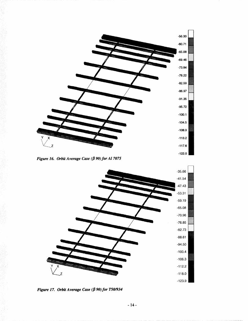
Figure 16. Orbit Average Case (fl 90)for A1 7075

/!i?iili_ii_!i/

/ii ii!iiiill

iii:iif:!_

Y X

Figure 17. Orbit Average Case (fl 90)for T50/934

-_.08

.69._

-73.:_

-78.22

-82.59

-86.97

-91 ._

-95,72

- 1_. 1

-104.5

-108.9

-113,2

-117.6

-1_,0

-35.66

-41.54

-47.43

-53.31

-59.19

-65.08

-70.96

-76.85

-82.73

-88.61

-94.50

-100.4

-106.3

-112.2

-118.0

-123.9

iiiiii!ii?iiiiiiiiiiii!!@!iiii!i:il

iiii!!!iiii!iii,,ii_!iii!ill:

!::_iii!_iiiii,

ili!!ii!:i_!i_:

:iii:!ili:iii!I::

Y X

Figure 18. Orbit Average Case (fl 90)for XN70

-61.62

-65.43

-69.25

-73.06

-76.87

-80.69

-84.50

-88.31

-92.12:

-95.94

-99.75

-103.6

-107.4

-111.2

-115.0

-118.8

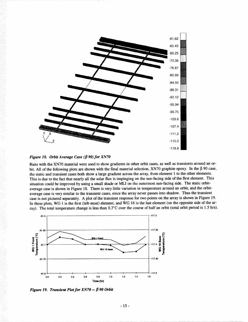
Runs _th the XNT0 material were used to show gradients in other orbit cases, as well as transients around an or-

bit. All of the following plots are shown :_th the final material selection, XN70 graphite epoxy. In the 1390 case,

the static and transient cases _th show a large gradient across the _ay, #om element I to the other elements.

This is due to the fact that nearly all the solar flux is impinging on the sun-facing side of the first element. This

situation could be improved by using a small shade or _I on the outermost sun-facing side. The static orbit-

average case is sho_ in Figure 18. There is very little variation in temperature around an orbit, and the orbit-

average case is very si_lar to the transient cases, since the _ay never passes into shadow. Thus the transientcase is not pictured separately. A plot of the transient response for two points on the _ay is shown in Figure 19.

In these plots, WG 1 is the first (le_-most) element, and WG 16 is the last element (on the opposite side of the ar-ray). The total temperature change is less than 0.3°C over the course of half an orbit (total orbit period is 1.5 hrs).

-61.6

-61.65

oo

=_"e_

tLm -61.7

,i@

I"

-61.75

-61.8

0.0

-117.3

l -117.35

I ®-117.4 _ •

Q

-117.45

I I I I I I I -117.5

0.2 0.4 0.6 0.8 1.0 1.2 1.4 1.6

Time (hr)

Figure 19. Transient Plot for XN70 -- fl 90 Orbit

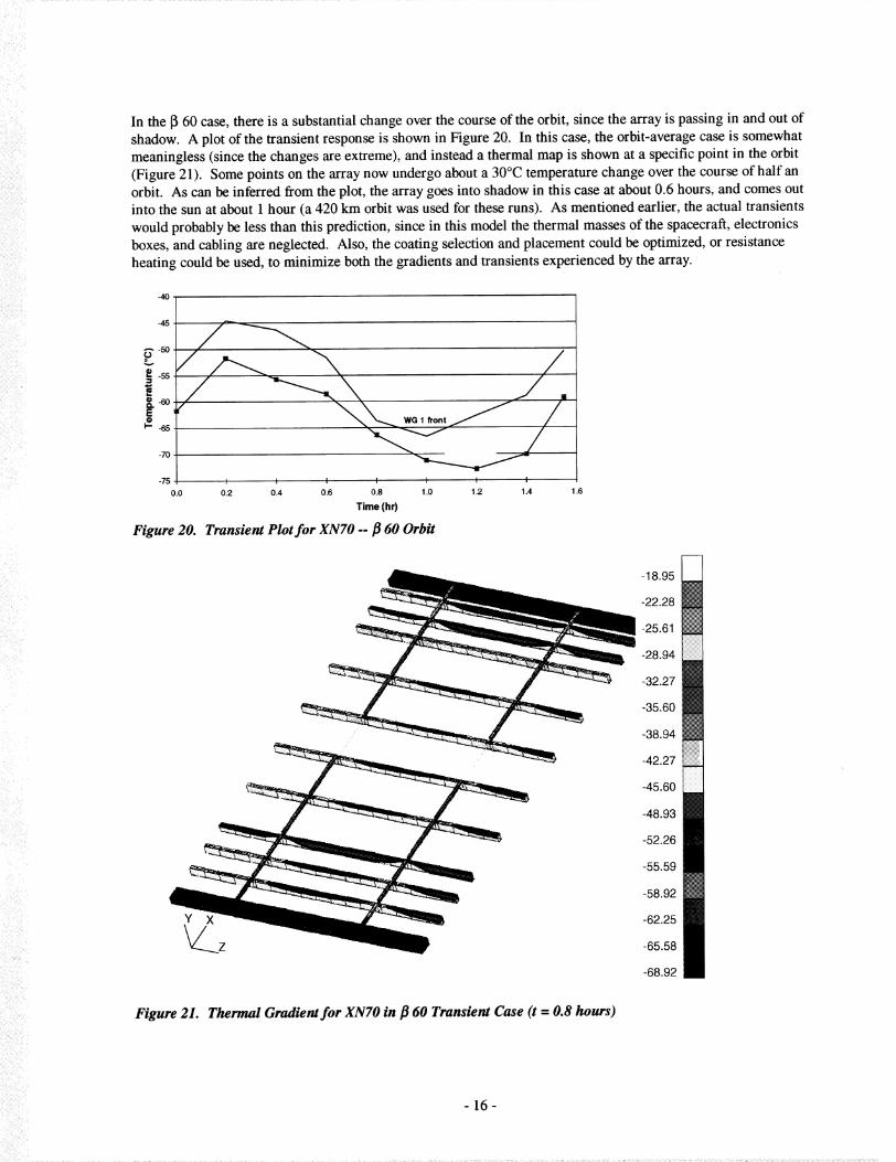
In the 13 60 case, there is a substantial change over the course of the orbit, since the array is passing in and out of

shadow. A plot of the transient response is shown in Figure 20. In this case, the orbit-average case is somewhat

meaningless (since the changes are extreme), and instead a thermal map is shown at a specific point in the orbit

(Figure 21). Some points on the array now undergo about a 30°C temperature change over the course of half an

orbit. As can be inferred from the plot, the array goes into shadow in this case at about 0.6 hours, and comes out

into the sun at about 1 hour (a 420 km orbit was used for these runs). As mentioned earlier, the actual transients

would probably be less than this prediction, since in this model the thermal masses of the spacecraft, electronics

boxes, and cabling are neglected. Also, the coating selection and placement could be optimized, or resistance

heating could be used, to minimize both the gradients and transients experienced by the array.

-40

-45

--- -50

oov

E

P" -65

-70

WG 1 front

1.2 1.4 t.6

-75

0.0 0.2 0.4 0.6 0.8 1.0

Time(hr)

Figure 20. Transient Plot for XN70 -- fl 60 Orbit

Y x

-18.95

-22.28

-25.61

-28.94

-32.27

-35.60

-38.94

-42.27

-45.60

-48.93

-52.26

-55.59

-58.92

-68.92

Figure 21. Thermal Gradient for XN70 in fl 60 Transient Case (t = 0.8 hours)

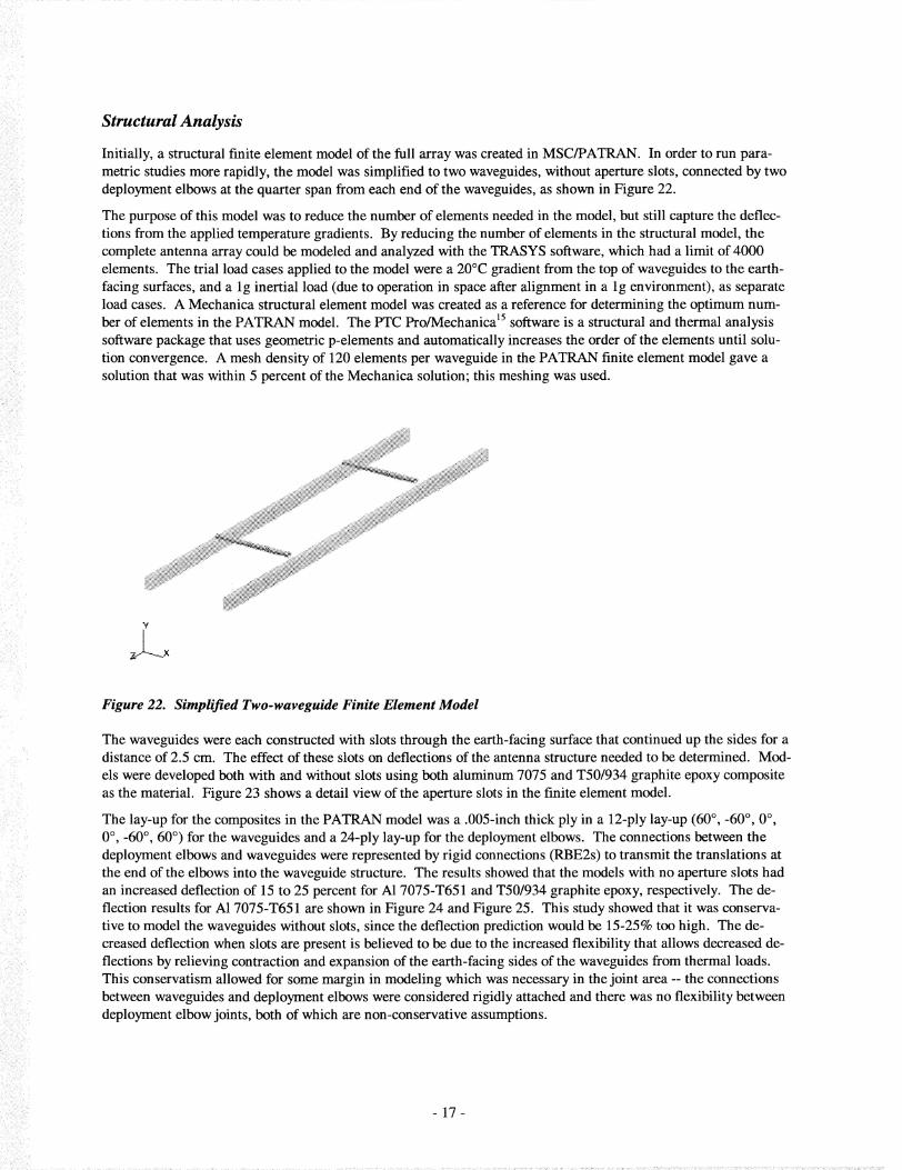
Structural Analysis

Initially, a structural finite element model of the full array was created in MSC/PATRAN. In order to run para-

metric studies more rapidly, the model was simplified to two waveguides, without aperture slots, connected by two

deployment elbows at the quarter span from each end of the waveguides, as shown in Figure 22.

The purpose of this model was to reduce the number of elements needed in the model, but still capture the deflec-

tions from the applied temperature gradients. By reducing the number of elements in the structural model, the

complete antenna array could be modeled and analyzed with the TRASYS software, which had a limit of 4000

elements. The trial load cases applied to the model were a 20°C gradient from the top of waveguides to the earth-

facing surfaces, and a lg inertial load (due to operation in space after alignment in a 1g environment), as separate

load cases. A Mechanica structural element model was created as a reference for determining the optimum num-ber of elements in the PATRAN model. The PTC Pro/Mechanica 15software is a structural and thermal analysis

software package that uses geometric p-elements and automatically increases the order of the elements until solu-

tion convergence. A mesh density of 120 elements per waveguide in the PATRAN finite element model gave a

solution that was within 5 percent of the Mechanica solution; this meshing was used.

_iiii_ii_ii__i_, .i _ ,!i!i_

ill_!!_i!il_i_ii_i_/!:i!!i_il

......_iiiiiii_iiiiiii!iii!i!__.......... ........._i_iiiiiiiiiiiiii!iiiii!ii_!_'

¥

,_.,-_---__.Y.:

Figure 22. Simplified Two-waveguide Finite Element Model

The waveguides were each constructed with slots through the earth-facing surface that continued up the sides for adistance of 2.5 cm. The effect of these slots on deflections of the antenna structure needed to be determined. Mod-

els were developed both with and without slots using both aluminum 7075 and T50/934 graphite epoxy composite

as the material. Figure 23 shows a detail view of the aperture slots in the finite element model.

The lay-up for the composites in the PATRAN model was a .005-inch thick ply in a 12-ply lay-up (60 °, -60 °, 0 °,

0 °, -60 °, 60 °) for the waveguides and a 24-ply lay-up for the deployment elbows. The connections between the

deployment elbows and waveguides were represented by rigid connections (RBE2s) to transmit the translations at

the end of the elbows into the waveguide structure. The results showed that the models with no aperture slots had

an increased deflection of 15 to 25 percent for A1 7075-T651 and T50/934 graphite epoxy, respectively. The de-

flection results for A1 7075-T651 are shown in Figure 24 and Figure 25. This study showed that it was conserva-

tive to model the waveguides without slots, since the deflection prediction would be 15-25% too high. The de-

creased deflection when slots are present is believed to be due to the increased flexibility that allows decreased de-

flections by relieving contraction and expansion of the earth-facing sides of the waveguides from thermal loads.

This conservatism allowed for some margin in modeling which was necessary in the joint area -- the connections

between waveguides and deployment elbows were considered rigidly attached and there was no flexibility between

deployment elbow joints, both of which are non-conservative assumptions.

-17-

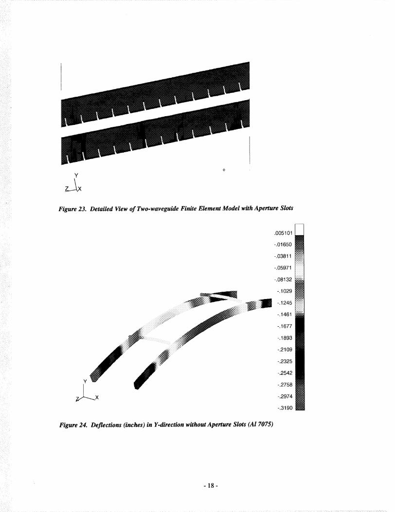
Figure 23. Detailed View of Two.waveguide Finite Element Model with Aperture S_ts

........._ i

.005101

-.01650

-.03811

-.05971

-.08132

-.1029

-.1245

-.1461

-.1677

-.1893

-.2109

-.2325

-.2542

-.2758

-.2974

-.3190

Figure 24. Deflections (inches) in Y.direction w#ho_ Aperture Slots (Al 7075)

.01312

-.005764

-.02465

-.04354

-.O6243

_i_ii!!!i__i_i,

//iiiii__i i_i:_!i

....... _i i_

!i

iiii_ii!!i_iliiiii_iiiil_i_i!!i_il/i__iiii_ii_i:_:_i_

.......iiiiii!ilil _ ii::_iii!iiiiiiiii_ iiii;iiiiiiiiiiiiiiiii........

J__x

-.08132

-.1002

-.1191

-. 1380

-.1569

-.1758

-. 1946

-.2135

-.2324

-.2513

-.2702

Figure 25. Deflections (inches) in Y.direction w#h Aperture Slots (A1 7075)

The structural analyses were then performed on the _,ll anmnna _ay, using the same PAT_ model employed

in the thermal analysis, without slots. The M 7075 and XN70 materials' deflection for _th the [_ 90 static tem-

perature gradient and orbit transient cases were compared. The lay-up for the composites in the _I1 PATRANmodel was the same as in the two-waveguide model. For A1 7075 the maximum deflection was 2.00 cm normal to

the plane of the element _ay. The maximum out-of-plane deflections for the composite models were 0.95 cm for

T50/934 carbon-epoxy composite and 0._3 cm for XN70. The property that has the most impact on the array

deflection is the c_fficient of thermal expansion (CTE or ix), which is shown in Table 9.

Deformation analyses were performed using both M 7075 and XN70 to deter_ne the transient deflection in orbit.The orbit transient deflection is the maximum variation in deflection that occurs as a result of temperature changes

around a [_ 60 orbit. The [_ 60 orbit transient deflections proved to _ more severe than [3 90 transient _flectionsdue to the increased thermal transient over an orbit. The maximum transient deflection is 0..80 cm for AI 7075 and

0.004 cm for XN70 (sho_ in Figure 26). These deflections are baseA on the structure being perfectly constructed;

i.e., there are no inaccuracies in the angle of layup or in the fiber angles, no asymmetry in the layer thic_esses,

etc.

From the results of the deformation analyses, XN70 achieves the smallest deformations by a significant margin

when compared with the M 7075 and the T50/934 composite. Other properties that lend XN70 to space applica-

tions on arrays are that it is more resis_t to _crocrac_ng than carbo_epoxy composites, which improves the

dimensional stability, and _at the lay-up of XN70 can be _lored so that the C_ of the composite is near zero.

i i_i_i

Table 9. Material Properties

Property

_11

c_22

Ell

E22

G12

V12

XN70 Laminate

-0.6 x 10 -6 in/in/°F

16.0 x 10 -6 in/in/°F

58.0 Msi

1.0 Msi

0.6 Msi

0.30

XN70 Lay-up (-60, 60, 0, 0, 60,-60)

-0.238 x 10 .6 in/in/°F

-0.238 x 10 -6 in/in/°F

20.2 Msi

20.2 Msi

7.61 Msi

0.30

.065 lbs/cu in

Property

cxll

22

Ell

E22

G12

V12

P

T50/934 Laminate

0.05 X 10 -6 in/in/°F

16.0 x 10 -6 in/in/°F

37.0 Msi

1.3 Msi

0.66 Msi

0.31

T50/934 Lay-up(-60,60, 0, 0, 60,-60)

4.73 x 10 .6 in/in/°F

4.73 x 10 -6 in/in/°F

16.7 Msi

16.7 Msi

5.76 Msi

0.31

.05 lbs/cu in

G

V

AI 7075-T651

12 x 10 -6 in/in/°F

10.3 Msi

3.9 Msi

.33

- 20-

.O01550

.001438

.001326

.001214

.001102

.0009900

.0008780

•0007659

.0006538

•0005418

•0004297

.0003176

.0002056

Y .00009350

_...x -.00001856

Figure 26. Transient Y.deflections (inches)for XN70 Antenna Array (fl 60 orbit)

-.0001306

Conclusions

Using electronically integrated three-dimensional analysis modeling software (MSC/PATRAN), thermal analyzers(SINDA-85, TRASYS, P/Thermal), and structural analysis software (MSC/NASTRAN), parametric analyses of a

16-element waveguide space radiometer array were performed. Several surface coatings, several base materials,and two orbital extreme cases were analyzed, both for transient and orbit-average behavior. The orbit altitude was

evaluated and found to have little impact on the results. The results of the analyses showed that the [3 60 orbit pro-

duced the worst-case thermal transient, while the _ 90 orbit produced the worst thermal gradient. Limited optimi-

zation of the surface coating layout was achieved with a combination of AI, A1-SiO2 MLI and Kapton MKI materi-als. It was shown that thermal gradients across the array were reduced significantly by use of a high conductivity

XN70 carbon-reinforced polycyanate composite as compared to a standard graphite-epoxy (T50/934) and alumi-

num alloy 7075. The requirements on maintenance of orientation and position for the array are difficult to meet

for an array of this size. The integrated analysis resulted in significant reduction of thermally driven deformations

using the XN70 material. It was demonstrated that parametric studies and optimization of complex space arrays

seeking minimum distortion can be accomplished using integrated thermal/structural techniques. A methodology

for future improved optimization is identified.

Acronyms

AgTFE

CTE

ESTAR

Silver-Teflon

Coefficient of Thermal Expansion

Electronically Scanned Thinned Array Radiometer

!i_iiiiiii!iiiiii_iiiiiiiiii!iii_iii_iii!i!_iii!iiiii_I!

i!i_!!!iiii!iiiii!_iiiiiii!!iiii

iiii!iii!ii!!!ii_!i!iii__

_i!iii_!i_ii_i!ii!ii__

MLI

RBE2

SOAP

VDA

WG

Multi-layer Insulation

Rigid Body Element (Form 2)

Sun-synchronous Orbit Analysis Program

Vapor deposited aluminum

Waveguide

References

LeVine, D.M., Wilheit, T.T. Jr., Murphy, R.E. ,and Swift, C.T., "A Multifrequency Microwave Radiometer of

the Future," IEEE Trans. Geosci. Remote Sensing, Vol. 27, No. 2, pp. 193-199, March 1989.

2 Jackson, T.J., et.al., "Soil Moisture and Rainfall Estimation Over a Semiarid Environment with the ESTAR Mi-

crowave Radiometer," IEEE Trans. Geosci. Remote Sensing, Vol. 31, No. 4, pp. 836-841, July 1993.

3 Fujioka, J.K. and Ely, W., Development of the SEASAT-A Satellite Scatterometer Antenna, NASA Contractor

Report 145299, February 1978.

4 LeVine, D.M., ICESTAR: A Microwave Radiometer to Support Arctic Navigation and Polar Process Studies,

NASA Goddard Space Flight Center white paper, January 1994.

Mutton, P., et. al., A Conceptual Study for a Two-Dimensional, Electronically Scanned Thinned Array Radi-

ometer, NASA TM- 109051, November, 1993.

ii_iiiii_ili_ii!!_' ii_ii!iiii!!_iiil,iiiii__i_

_i,_i,_ _ i

6 Gould, D. C., A Conceptual Thermal Design Study of an Electronically Scanned Thinned Array Radiometer,

NASA TM-110173, May 1995.

7 Birky, A.K., et.al, Hydrostar Engineering Feasibility Report, Swales and Associates for NASA GSFC, February

2, 1995.

8Le Vine, D.M. and Weissman, D.E., "Calibration of Synthetic Aperture Radiometers in Space: Antenna Effects",

Proc. IGARSS-96, Vol II, pp. 878-880, Lincoln, Nebraska, May 1996.

9 Tanner, A.., Swift, C., "Calibration of a Synthetic Aperture Radiometer," IEEE Trans. Geo. and Remote Sens.,

Vol 31, No. 1, pp. 257-267, January 1993.

10Killough, B. D., Thermal and Orbital Analysis of Earth Monitoring Sun-Synchronous Space Experiments,

NASA TM- 101630, May 1990.

/_ _i_ii_!iiii_,i_'!

_i!,_ii•i_ii!!i_il

11Thermal Radiation Analyzer System (TRASYS) User's Manual, JSC-22964, April 1988.

12 SINDA '85/FLUINT, Systems Improved Numerical Differencing Analyzer and Fluid Integrator, Version 2.3,

MCR-90-512, August 1986.

13MSC/PATRAN User Manual, MacNeal-Schwendler Corporation, Version 5.0 (March 1996) and 6.0 (August

1996).

i4 Silverman, E. M. (Compiler), Composite Structures Design Guide, NASA Contractor Report 4708, March 1996.

15Parametric Technology Corporation, Pro/Mechanica Reference Manual, 1997.

i_ ilil !•ii_!iii:iiii_:'

'ii!ii!_iii_iiiiiii!illi_i_

!i!!!i%ii__i__iiii!i_iiii!i!_iiiii_i_ii_

i_i_i!i_ii_!_iii_ili_iiii_,_!_i__i_ii!iii:i'_II_

- 22-

, _ii_:_!i_,_!:I,;?!L,_I:I_;?_,_,I!!_i_ii_iii'Lii_;_• _:_ '?_'_i.... i ii:i_;¸¸!II!_

• ,'.(_ _i__ 'i:_ _,_i_i:_; iii__i_A :_:

REPORT DOCUMENTATION PAGEForm ApprovedOMB No. 0704-0188

Public reporting burden for this collection of information is estimated to average 1 hour per response, including the time for reviewing instructions, searching existing datasources, gathering and maintaining the data needed, and completing and reviewing the collection of information. Send comments regarding this burden estimate or any otheraspect of this collection of information, including suggestions for reducing this burden, to Washington Headquarters Services, Directorate for Information Operations andReports, 1215 Jefferson Davis Highway, Suite 1204, Arlington, VA 22202-4302, and to the Office of Management and Budget, Paperwork Reduction Project (0704-0188),Washington, DC 20503.

1. AGENCY USE ONLY (Leave blank) 2. REPORT DATE

February 1998

3. REPORT TYPE AND DATES COVERED

Technical Memorandum

4. TITLE AND SUBTITLE

Hydrostar Thermal and Structural Deformation Analyses of Antenna Array

Concept

6. AUTHOR(S)

Ruth M. Amundsen, Drew J. Hope

7. PERFORMING ORGANIZATION NAME(S) AND ADDRESS(ES)

NASA Langley Research Center

Hampton, VA 23681-2199

9. SPONSORING/MONITORING AGENCY NAME(S) AND ADDRESS(ES)

National Aeronautics and Space AdministrationWashington, DC 20546-0001

5. FUNDING NUMBERS

632-10-14-37

8. PERFORMING ORGANIZATION

REPORT NUMBER

L-17679

10. SPONSORING/MONITORING

AGENCY REPORT NUMBER

NASA/TM- 1998-206288

11. SUPPLEMENTARY NOTES

12a. DISTRIBUTION/AVAILABILITY STATEMENT 12b. DISTRIBUTION CODE

Unclassified-Unlimited

Subject Category 18 Distribution: StandardAvailability: NASA CASI (301) 621-0390

13. ABSTRACT (Maximum 200 words)

The proposed Hydrostar mission used a large orbiting antenna array to demonstrate synthetic aperturetechnology in space while obtaining global soil moisture data. In order to produce accurate data, the array wasrequired to remain as close as possible to its perfectly aligned placement while undergoing the mechanical andthermal stresses induced by orbital changes. Thermal and structural analyses for a design concept of this

antenna array were performed. The thermal analysis included orbital radiation calculations, as well asparametric studies of orbit altitude, material properties and coating types. The thermal results included predictedthermal distributions over the array for several cases. The structural analysis provided thermally-drivendeflections based on these cases, as well as based on a 1-g inertial load. In order to minimize the deflections ofthe array in orbit, the use of XN70, a carbon-reinforced polycyanate composite, was recommended.

14. SUBJECT TERMS

thermal, structural, analysis, thinned array, antenna, orbiting antenna,

soil moisture, synthetic aperture technology, space, composite waveguide

17. SECURITY CLASSIFICATION

OF REPORT

Unclassified

18. SECURITY CLASSIFICATION

OF THIS PAGE

Unclassified

19. SECURITY CLASSIFICATION

OF ABSTRACT

Unclassified

15. NUMBER OF PAGES

28

16. PRICE CODE

A03

20. LIMITATION

OF ABSTRACT

NSN 7540-01-280-5500 Standard Form 298 (Rev. 2-89)

Prescribed by ANSI Std. Z-39-18298-102