Hydromorphology of an urbanizing watershed 10-26-06engineering.tufts.edu/cee/people/vogel/documents/hydromorphology... · October 26, 2006 Advances in Water Resources Under Review

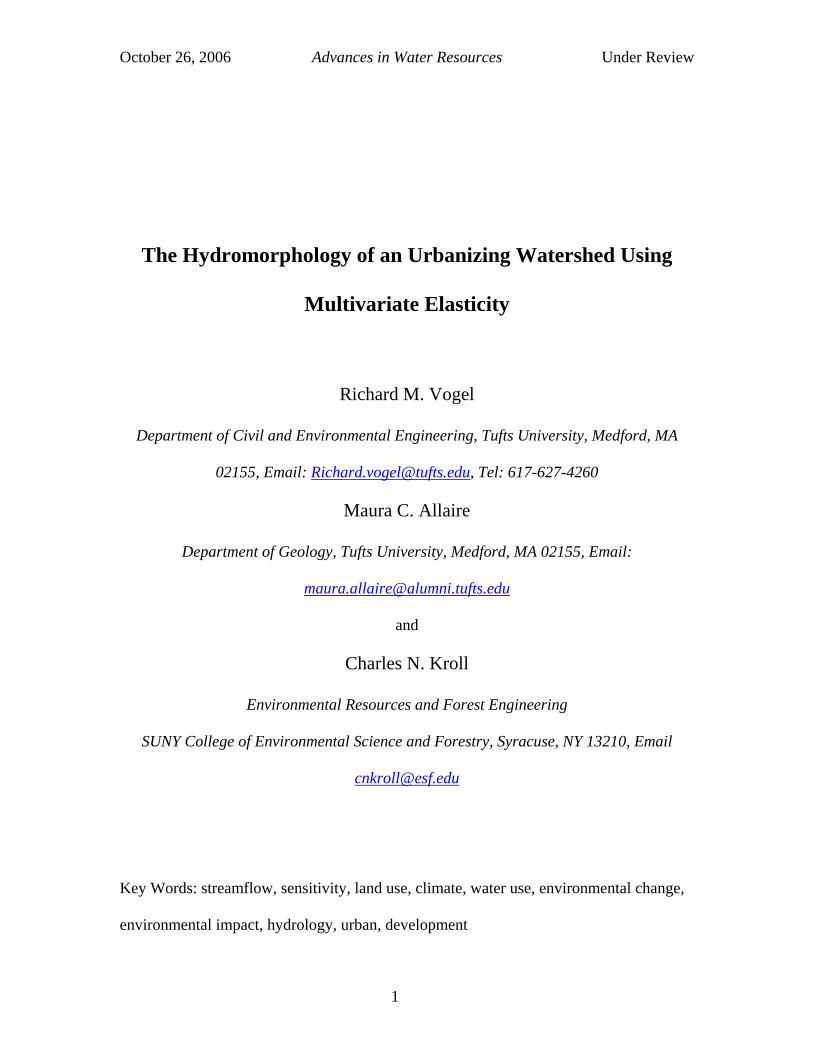
October 26, 2006 Advances in Water Resources Under Review

1

The Hydromorphology of an Urbanizing Watershed Using

Multivariate Elasticity

Richard M. Vogel

Department of Civil and Environmental Engineering, Tufts University, Medford, MA

02155, Email: [email protected], Tel: 617-627-4260

Maura C. Allaire

Department of Geology, Tufts University, Medford, MA 02155, Email:

[email protected]

and

Charles N. Kroll

Environmental Resources and Forest Engineering

SUNY College of Environmental Science and Forestry, Syracuse, NY 13210, Email

[email protected]

Key Words: streamflow, sensitivity, land use, climate, water use, environmental change,

environmental impact, hydrology, urban, development


2

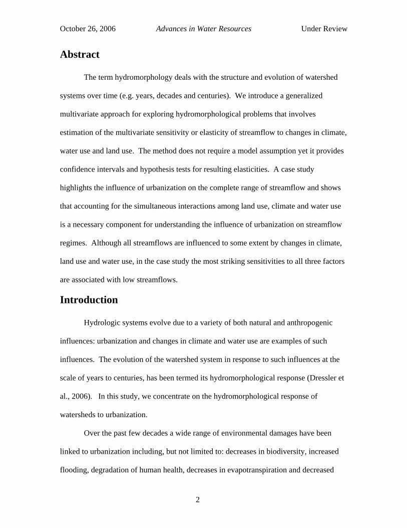
Abstract

The term hydromorphology deals with the structure and evolution of watershed

systems over time (e.g. years, decades and centuries). We introduce a generalized

multivariate approach for exploring hydromorphological problems that involves

estimation of the multivariate sensitivity or elasticity of streamflow to changes in climate,

water use and land use. The method does not require a model assumption yet it provides

confidence intervals and hypothesis tests for resulting elasticities. A case study

highlights the influence of urbanization on the complete range of streamflow and shows

that accounting for the simultaneous interactions among land use, climate and water use

is a necessary component for understanding the influence of urbanization on streamflow

regimes. Although all streamflows are influenced to some extent by changes in climate,

land use and water use, in the case study the most striking sensitivities to all three factors

are associated with low streamflows.

Introduction

Hydrologic systems evolve due to a variety of both natural and anthropogenic

influences: urbanization and changes in climate and water use are examples of such

influences. The evolution of the watershed system in response to such influences at the

scale of years to centuries, has been termed its hydromorphological response (Dressler et

al., 2006). In this study, we concentrate on the hydromorphological response of

watersheds to urbanization.

Over the past few decades a wide range of environmental damages have been

linked to urbanization including, but not limited to: decreases in biodiversity, increased

flooding, degradation of human health, decreases in evapotranspiration and decreased


3

quality of air, water and soil resources. The hydrologic effects of urbanization are

primarily a result of both continuous and abrupt land-use and infrastructure changes that

lead to changes in the land and the atmospheric component of the hydrologic cycle as

well as changes in the water use cycle. Urbanization leads to the construction of water

distribution systems, as well as an infrastructure to accommodate storm water and

sewage. All of these modifications to the landscape result in changes to the hydrologic

cycle and watershed processes. There has been a wide range of initiatives relating to

watershed management to ameliorate past damages and/or prevent future environmental

damages resulting from the urbanization of watersheds. Essentially, watershed systems

evolve due to changes in land-use, climate, and an array of other anthropogenic

influences.

There have been a variety of efforts to quantify the changes in watershed land-

use, biodiversity and other aspects of watershed evolution (Firbank et al., 2003). There is

also increased attention focused on improving our understanding of the impacts of

urbanization on stream and watershed ecosystems (Nilsson, et al., 2003) and this area will

receive increased attention in the future (DeFries and Eshleman, 2004). Most previous

evaluations of the hydrologic impact of urbanization have focused on flood hydrology

(Leopold, 1968; Brater and Sangal, 1969). For instance, Beighley et al. (2003) found that

urbanization increases both peak discharges and flood runoff volumes while decreasing

their associated variability. Choi et al. (2003) found that urbanization leads to greater

impacts on direct (flood) runoff than total (average) runoff. Similarly, Cheng and Wang

(2002) quantified the impact of imperviousness on both the flood peak magnitude and the

time of concentration. Beighley and Moglen (2002, 2003) also focus on the impact of

urbanization on flood hydrology. They developed methods for adjusting observed time-


4

series of flood peaks to enable one to estimate the frequency of floods under current land-

use conditions.

Fewer studies have focused on the impacts of urbanization on average runoff and

even fewer on low flows. Grove et al. (2002) found increases in average annual runoff of

more than 60% resulting from urbanization influences during the period 1973 to 1991 for

an urbanizing basin near Indianapolis, Indiana. Bhaduri et al. (2001) obtained similar

results. In a more comprehensive study for basins across the entire U.S., DeWalle et al.

(2000) concluded that urbanization increased mean annual streamflow in rough

proportion to average cumulative changes in population density. Dow and DeWalle

(2000) review a number of additional studies all of which concluded that the primary

response of a watershed to increasing urban land use is an increase in surface runoff.

However, Dow and DeWalle (2000) also document significant decreases in watershed

evapotranspiration that result from urbanization which is consistent with the results of

this study. Claessens et al. (2006) use a monthly water balance model to show that it is

necessary to understand the interactions among climate, land use and water use to predict

the streamflow regime in an urbanizing watershed.

Schilling and Libra (2003) found that in nearly all watersheds evaluated in Iowa;

annual baseflow, annual minimum flow and annual baseflow percentage of flow all

increased over time. They suggest that these increases may result from improved land

management and conservation practices. Snodgrass et al. (1997) and Brandes et al.

(2005) cite numerous studies which obtain conflicting results, some concluding that

urbanization increases low streamflows and others concluding that it decreases low

streamflows. On the one hand, Leopold (1968), Dunne and Leopold (1978), Klein

(1979), Shaw (1994), Barringer et al. (1994), Rose and Peters (2001), Paul et al. (2001)


5

and many others have argued that urbanization will tend to increase baseflow . On the

other hand, Hollis (1977), Snodgrass et al. (1997), Lerner (2002), Meyer (2002, 2005)

and Brandes et al. (2005) documented increases in low flows resulting from urbanization.

Meyer (2002) found that urbanization increased low flows due to leakage from water,

stormwater and sewer systems. Similarly, Lerner (2002) found that leaks from water

distribution systems led to increases in groundwater recharge and resulting low flows.

The study by Leopold (1968) is one of the most comprehensive reports on the

hydrologic impact of urbanization because it uses cited literature and actual data to arrive

at conclusions regarding the generalized impacts of urbanization on flood peaks, flood

volumes, sediment discharge, and water quality. However, that study only concentrated

on the impact of urbanization on flood hydrology, whereas this study attempts to focus on

the entire hydrologic cycle. Interestingly, Leopold (1968), Dunne and Leopold (1978),

Shaw (1994), Rose and Peters (2001) and many others have argued that urbanization, or

increasing impervious area, causes decreases in groundwater recharge and baseflow.

This is counter to the results of Hollis (1977), Snodgrass et al. (1997), Lerner (2002),

Meyer (2002, 2005), and Brandes et al. (2005) as well as the results of this study.

Study Goals:

There is a general consensus in the literature regarding some of the

hydromorphologic impacts of urbanization. It is generally agreed that urbanization will

lead to increases in direct runoff and thus increases in floods. It is not clear whether

urbanization will cause increases or decreases in baseflow and resulting low streamflows.

Increases in baseflow may result from leakage of urban water infrastructure as well as

due to decreases in evapotranspiration that result from replacing vegetation with urban

infrastructure. In addition, urbanization may produce changes in groundwater recharge


6

due to changes in the hydraulic routing of water over the landscape. Decreases in

baseflows may result from reductions in infiltration due to replacement of vegetation with

urban infrastructure and due to exfiltration of soil water into sewer and stormwater

systems. Trends in climate, land use and water use within a basin will also lead to

associated trends in streamflows. We hypothesize, as did Claessens et al. (2006), that

urbanization processes which influence low to average streamflow are extremely

complex and can result in simultaneous increases and decreases in low to average

streamflow due to the complicated interactions among climate, land use, water use and

water infrastructure. This study does not purport to provide a definitive answer to the

question of how urbanization impacts low flow. Rather, our primary goal is to inspire

others to use the methodology introduced here to examine various hypotheses relating to

the impact of both natural and anthropogenic influences on the hydrologic cycle. Further,

our goal is to demonstrate that one can only understand the interactions among land use,

climate and water use in an urban watershed if these factors are considered in an

integrated fashion.

There is clearly an increasing interest in the impacts of urbanization on the

hydrologic cycle, and it is no longer sufficient to focus solely on the impacts of

urbanization on flood events as is so common in the past. The methodology introduced

in this study is quite general and should have application to a wide range of problems in

hydrology that seek to evaluate the hydromorphological response of a watershed to both

natural and anthropogenic influences. After presenting the methodology, a case study is

introduced which evaluates the generalized hydrologic impacts of urbanization focusing

on the entire hydrologic cycle of an urbanizing watershed in the suburbs of Boston.


7

The Generalized Sensitivity or Elasticity of Streamflow to

Changes in Climate, Land Use and Water Use

Previous hydrologic investigators introduced the concept of precipitation

elasticity to examine the generalized sensitivity of streamflow to changes in precipitation

(Schaake, 1990; Sankarasubramanian et al. 2001; Chiew, 2006). The precipitation

elasticity of streamflow is defined as the proportional change in streamflow Q divided by

the proportional change in precipitation P:

QP

dPdQ

PdPQdQ

P ==ε (1)

Sankarasubramanian et al. (2001) found it useful to define elasticity at the mean value of

the climate variable so that

QP

dPdQ

P =ε (2)

The interpretation of elasticity is quite simple. For example, if εp = 2 for annual

streamflows, then a 1% change in precipitation leads to a 2% change in streamflow.

Sankarasubramanian et al. (2001) introduced a nonparametric estimator of the

precipitation elasticity that was shown to have desirable statistical properties; however, it

is only suited to determine the sensitivity of streamflow to changes in a single

explanatory variable. We desire a multivariate nonparametric estimator of elasticity to

examine the sensitivity of streamflow to changes in climate, land use and water use,

simultaneously. The following section describes a general approach to multivariate

elasticity of streamflow for use in hydromorphological studies.


8

Multivariate Climate/WaterUse/LandUse Elasticity of Streamflow

We wish to determine the generalized sensitivity of streamflow Q, to changes in

precipitation P, land use L, and water use W. Consider the total differential of

streamflow resulting from simultaneous changes in P, L, and W

WWQdL

LQdP

PQdQ ∂

∂∂

+∂∂

+∂∂

= (3)

Following the recommendation of Sankarasubramanian et al. (2001), estimation of the

differentials around the mean values of each variable in (3) leads to

( ) ( ) ( )WWWQLL

LQPP

PQQQ −

∂∂

+−∂∂

+−∂∂

=− (4)

Dividing each term in (4) by Q , and multiplying the three terms on the right hand side

by unity in the form of PP , LL and WW , respectively, results in

⎟⎟⎠

⎞⎜⎜⎝

⎛ −∂∂

+⎟⎟⎠

⎞⎜⎜⎝

⎛ −∂∂

+⎟⎟⎠

⎞⎜⎜⎝

⎛ −∂∂

=⎟⎟⎠

⎞⎜⎜⎝

⎛ −W

WWQW

WQ

LLL

QL

LQ

PPP

QP

PQ

QQQ (5)

Now defining the lower case variables, q, p, l, and w as the four respective terms in

parenthesis in (5) (i.e. the percentage of change from the mean) we obtain

wlpq WLP ⋅+⋅+⋅= εεε (6)

where

QP

PQ

P ∂∂

=ε , QL

LQ

L ∂∂

=ε and QW

WQ

W ∂∂

=ε

are the precipitation, land use and water use elasticity of streamflow, respectively. Note

that Pε in (6) is identical to the definition of Pε in (2). The idea here is to employ

ordinary least squares (OLS) regression methods to fit the multivariate linear model in (6)


9

resulting in minimum variance, unbiased estimates of the three elasticities Pε , Lε and

Wε . The advantages of this approach to elasticity estimation are:

(1) The linear multivariate model in (6) is based on the definition of the total differential

(eq. 1) which is one of the most basic concepts of differential calculus, therefore,

there is no question whether or not the model is correct.

(2) The estimation method, multivariate ordinary least squares regression, has very

attractive properties, because resulting estimates of elasticity’s are unbiased, and

standard errors and confidence intervals for elasticities are available so that

hypothesis tests can be constructed. Corrections for heteroscedasticity (Stedinger and

Tasker, 1985; Kroll and Stedinger, 1998), autocorrelated model errors (Draper and

Smith, 1981) and other violations of OLS model assumptions (Johnston, 1984) are

also possible.

(3) Any number of additional explanatory variables may be added to the analysis and a t-

test may be performed to evaluate whether or not a hypothesized elasticity is

significantly different from zero, or not. In addition, one can assess which

explanatory variables impact streamflow changes the most via an examination of the

model sum of squared error contributed by each explanatory variable.

(4) The explanatory power of the regression in (6) (i.e. value of R2) is not preeminent as

is often the case in hydrologic analyses. Instead, what matters is that the residuals of

the model in (6) are independent with a constant variance and are normally

distributed, in which case, confidence intervals and hypothesis tests regarding the

elasticities have meaning.

(5) The meaning of the model parameter estimates in (6), termed elasticities, have an

interpretable meaning. For example, if an elasticity is near 0, the variable has no


10

impact on streamflow. If elasticity is near unity, the relation is linear. Larger or

smaller values indicate greater sensitivity to streamflow. Values either lower than or

in excess of unity imply a nonlinear response.

(6) Equation (6) can be applied in both time or space. In this study we study the elasticity

of a single watershed over time; however, the same type of analysis could be

performed by replacing ‘space’ for ‘time’ as is often done in hydrology. Such an

analysis would be analogous to the development of regional hydrologic regression

models which provide an approach to estimation of regional elasticities (see Vogel et

al. 1999, pg 152).

The Hydromorphology of an Urbanizing Watershed

The following is a case study which dramatizes the hydromorphological response

of a watershed to changes in climate, land use, and water use. Our case study begins with

an exploratory data analyses to frame the problem and is followed by the application of

equation (6) to evaluate the generalized hydromorphological response of an urbanizing

watershed. The 24 square mile urbanizing watershed is defined by the U.S. Geological

Survey streamflow gage on the Aberjona River at Winchester, Massachusetts (Gage

#001102500).

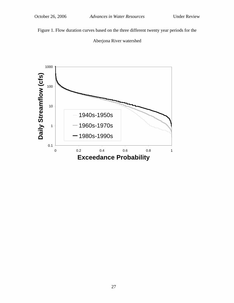
Exploratory Data Analysis: Flow duration curves (FDC’s) provide a simple,

general, graphical overview of the historical variability of streamflow in a watershed and

are useful for solving a wide range of water resource engineering problems (Vogel and

Fennessey, 1994, 1995). Figure 1 illustrates daily flow duration curves (FDC’s) for the

Aberjona River at Winchester constructed for three non-overlapping 20-year periods (1)

1940-1959, (2) 1960-1979 and (3) 1980-1999. The FDC’s in Figure 1 are developed


11

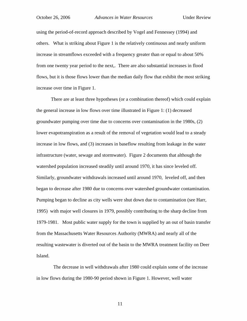
using the period-of-record approach described by Vogel and Fennessey (1994) and

others. What is striking about Figure 1 is the relatively continuous and nearly uniform

increase in streamflows exceeded with a frequency greater than or equal to about 50%

from one twenty year period to the next,. There are also substantial increases in flood

flows, but it is those flows lower than the median daily flow that exhibit the most striking

increase over time in Figure 1.

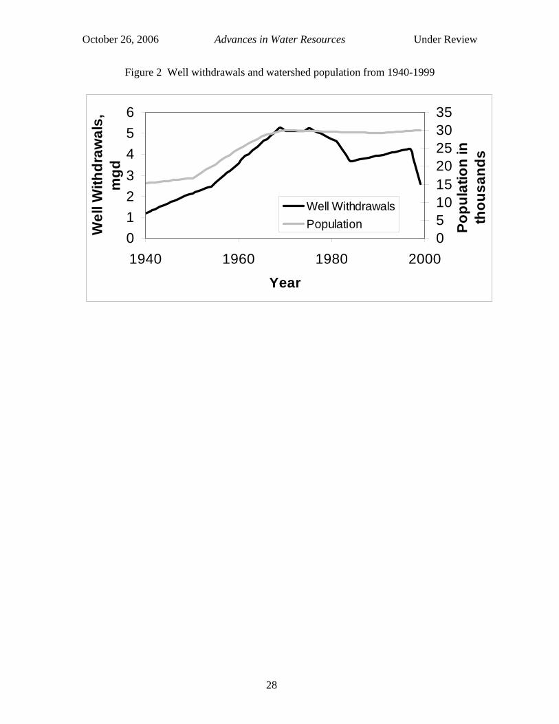
There are at least three hypotheses (or a combination thereof) which could explain

the general increase in low flows over time illustrated in Figure 1: (1) decreased

groundwater pumping over time due to concerns over contamination in the 1980s, (2)

lower evapotranspiration as a result of the removal of vegetation would lead to a steady

increase in low flows, and (3) increases in baseflow resulting from leakage in the water

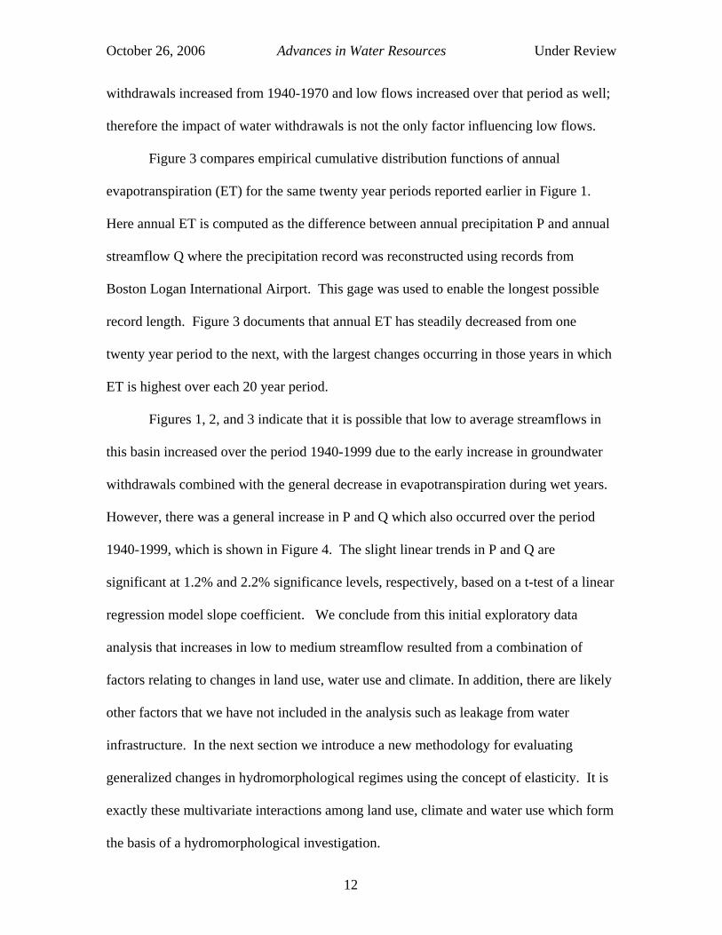
infrastructure (water, sewage and stormwater). Figure 2 documents that although the

watershed population increased steadily until around 1970, it has since leveled off.

Similarly, groundwater withdrawals increased until around 1970, leveled off, and then

began to decrease after 1980 due to concerns over watershed groundwater contamination.

Pumping began to decline as city wells were shut down due to contamination (see Harr,

1995) with major well closures in 1979, possibly contributing to the sharp decline from

1979-1981. Most public water supply for the town is supplied by an out of basin transfer

from the Massachusetts Water Resources Authority (MWRA) and nearly all of the

resulting wastewater is diverted out of the basin to the MWRA treatment facility on Deer

Island.

The decrease in well withdrawals after 1980 could explain some of the increase

in low flows during the 1980-90 period shown in Figure 1. However, well water


12

withdrawals increased from 1940-1970 and low flows increased over that period as well;

therefore the impact of water withdrawals is not the only factor influencing low flows.

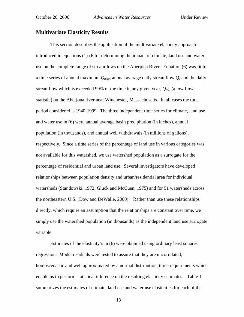
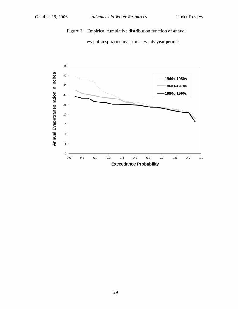
Figure 3 compares empirical cumulative distribution functions of annual

evapotranspiration (ET) for the same twenty year periods reported earlier in Figure 1.

Here annual ET is computed as the difference between annual precipitation P and annual

streamflow Q where the precipitation record was reconstructed using records from

Boston Logan International Airport. This gage was used to enable the longest possible

record length. Figure 3 documents that annual ET has steadily decreased from one

twenty year period to the next, with the largest changes occurring in those years in which

ET is highest over each 20 year period.

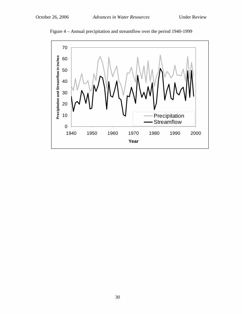
Figures 1, 2, and 3 indicate that it is possible that low to average streamflows in

this basin increased over the period 1940-1999 due to the early increase in groundwater

withdrawals combined with the general decrease in evapotranspiration during wet years.

However, there was a general increase in P and Q which also occurred over the period

1940-1999, which is shown in Figure 4. The slight linear trends in P and Q are

significant at 1.2% and 2.2% significance levels, respectively, based on a t-test of a linear

regression model slope coefficient. We conclude from this initial exploratory data

analysis that increases in low to medium streamflow resulted from a combination of

factors relating to changes in land use, water use and climate. In addition, there are likely

other factors that we have not included in the analysis such as leakage from water

infrastructure. In the next section we introduce a new methodology for evaluating

generalized changes in hydromorphological regimes using the concept of elasticity. It is

exactly these multivariate interactions among land use, climate and water use which form

the basis of a hydromorphological investigation.


13

Multivariate Elasticity Results This section describes the application of the multivariate elasticity approach

introduced in equations (1)-(6 for determining the impact of climate, land use and water

use on the complete range of streamflows on the Aberjona River. Equation (6) was fit to

a time series of annual maximum Qmax, annual average daily streamflow Q, and the daily

streamflow which is exceeded 99% of the time in any given year, Q99, (a low flow

statistic) on the Aberjona river near Winchester, Massachusetts. In all cases the time

period considered is 1940-1999. The three independent time series for climate, land use

and water use in (6) were annual average basin precipitation (in inches), annual

population (in thousands), and annual well withdrawals (in millions of gallons),

respectively. Since a time series of the percentage of land use in various categories was

not available for this watershed, we use watershed population as a surrogate for the

percentage of residential and urban land use. Several investigators have developed

relationships between population density and urban/residential area for individual

watersheds (Standowski, 1972; Gluck and McCuen, 1975) and for 51 watersheds across

the northeastern U.S. (Dow and DeWalle, 2000). Rather than use these relationships

directly, which require an assumption that the relationships are constant over time, we

simply use the watershed population (in thousands) as the independent land use surrogate

variable.

Estimates of the elasticity’s in (6) were obtained using ordinary least squares

regression. Model residuals were tested to assure that they are uncorrelated,

homoscedastic and well approximated by a normal distribution, three requirements which

enable us to perform statistical inference on the resulting elasticity estimates. Table 1

summarizes the estimates of climate, land use and water use elasticities for each of the


14

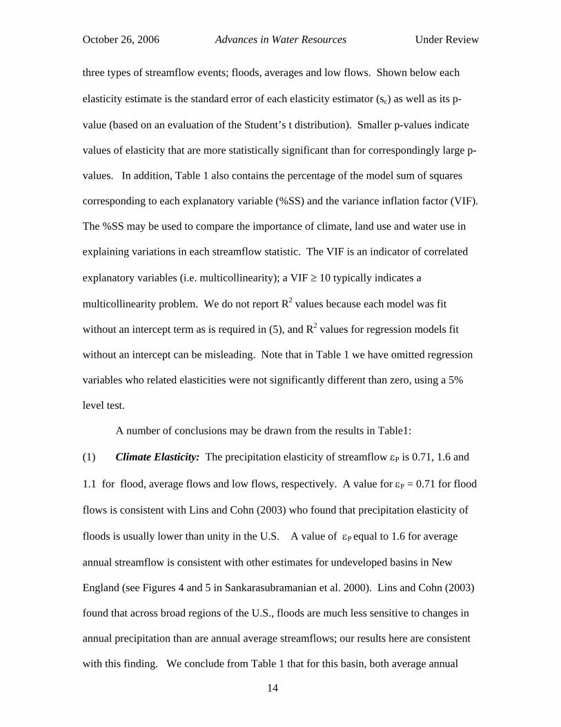
three types of streamflow events; floods, averages and low flows. Shown below each

elasticity estimate is the standard error of each elasticity estimator (sε) as well as its p-

value (based on an evaluation of the Student’s t distribution). Smaller p-values indicate

values of elasticity that are more statistically significant than for correspondingly large p-

values. In addition, Table 1 also contains the percentage of the model sum of squares

corresponding to each explanatory variable (%SS) and the variance inflation factor (VIF).

The %SS may be used to compare the importance of climate, land use and water use in

explaining variations in each streamflow statistic. The VIF is an indicator of correlated

explanatory variables (i.e. multicollinearity); a VIF ≥ 10 typically indicates a

multicollinearity problem. We do not report R2 values because each model was fit

without an intercept term as is required in (5), and R2 values for regression models fit

without an intercept can be misleading. Note that in Table 1 we have omitted regression

variables who related elasticities were not significantly different than zero, using a 5%

level test.

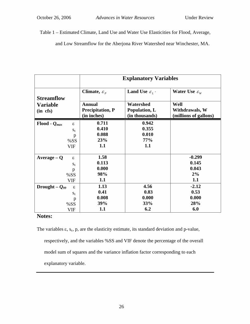
A number of conclusions may be drawn from the results in Table1:

(1) Climate Elasticity: The precipitation elasticity of streamflow εP is 0.71, 1.6 and

1.1 for flood, average flows and low flows, respectively. A value for εP = 0.71 for flood

flows is consistent with Lins and Cohn (2003) who found that precipitation elasticity of

floods is usually lower than unity in the U.S. A value of εP equal to 1.6 for average

annual streamflow is consistent with other estimates for undeveloped basins in New

England (see Figures 4 and 5 in Sankarasubramanian et al. 2000). Lins and Cohn (2003)

found that across broad regions of the U.S., floods are much less sensitive to changes in

annual precipitation than are annual average streamflows; our results here are consistent

with this finding. We conclude from Table 1 that for this basin, both average annual


15

flows and low flows are more sensitive to changes in annual rainfall than flood

discharges. These results imply that for this basin, future changes in precipitation will

tend to exacerbate average annual streamflows and droughts more than floods.

(2) Land Use Elasticity: The population (residential land use) elasticity of streamflow

εL is 0.94 and 4.6 for flood flows and low flows, respectively. The value of εL

associated with average flows was not significantly different from zero, hence we did not

report it in Table 1. Apparently, for this basin, changes in residential land use, as

evidenced by population growth, have had their greatest impact on low flows and floods,

with the greatest impact on low flows. It is common knowledge that increases in

residential land use tends to exacerbate floods, however to our knowledge, the extremely

large positive sensitivity of low flows to changes in land use shown in Table 1 has never

been shown before. While we are unable to say definitively why low flows are so

sensitive to urbanization, we are confident that climate, land use and water use all play

key roles, due to the relatively equal fractions of model sum of squares explained by each

of these explanatory variables. Further studies for a much wider class of basins and

urbanization levels are needed to support and generalize these findings.

(3) Water Use Elasticity: The water use elasticity of streamflow εW is -0.3, and -2.1 for

average flows and low flows, respectively. Water use elasticity of flood flows were not

significantly different from zero hence it is not reported in Table 1. As expected, well

withdrawals lead to decreases in streamflows. Once again, low flows are much more

sensitive to changes in water use than either floods or average flows.

(4) Variability of Elasticity Estimates: The relative variability of an elasticity estimate

can be measured by its coefficient of variation Cv, which is the inverse of the t-ratio from


16

which the p-value reported in Table 1 is derived. All the models are fit using the same

number of samples, in which case smaller p-values indicate model coefficients with low

variability (i.e. low p-values correspond to high t-ratios which implies low Cv associated

with model coefficients). Interestingly, the variability of all elasticity estimates in Table

1 are proportional to their associated elasticity values. In other words, the higher

elasticity values always had lower p-values and thus less variability (lower coefficient of

variation) than the lower values of elasticty. Thus, as streamflow sensitivity to climate,

land use and water use increases, so does our confidence in the results!

(5) Streamflow Sensitivity: The most statistically significant elasticity’s (smallest p-

values) and the largest values of elasticity were generally obtained for the low flow

statistic Q99. This implies that all three factors: climate, land use and water use have a

tremendous and highly significant impact on low flows. For example, an increase in

population of 1% will lead to a 4.56% increase in low flow. Similarly, a 1% annual

increase in well withdrawals will lead to 2.12% decrease in low flow. This is also

consistent with the results of recent trend studies which have shown that low flows tend

to exhibit the most consistent trends due to changes in climate than any other flow

statistic (Small et al., 2006).

(6) Multivariate Elasticity: Perhaps the most important conclusion arising from Table 1

is the fact that streamflow is sensitive to changes in climate, land use and water use, and

that all three of these effects must be considered simultaneously to fully understand the

hydromorphology of this watershed. To highlight this point, elasticity’s were computed

for Q99, based on simple regressions between each explanatory variable, separately. In

other words, the elasticities were estimated from the following three bivariate equations

pq P ⋅= ε , lq L ⋅= ε and wq W ⋅= ε individually, instead of the single multivariate


17

expression in (6). The resulting estimates of Pε , Lε and Wε for Q99 were 1.11, 1.15 and

0.526, respectively, compared to the values of 1.13, 4.56, and -2.12, respectively,

reported in Table 1. It makes little sense for the value of Wε to be greater than zero

because this would imply that an increase in water withdrawals leads to an increase in

low flow. We conclude, as did Claessens et al. (2006), that it is necessary to account for

the multivariate interactions among land use, climate and water use to fully understand

their impacts on streamflow.

Conclusions

Hydromorphology is defined as the structure and evolution of hydrologic systems.

Hydrologic systems tend to evolve in response to anthropogenic and climatic influences

which they are subject to, and as a result, nearly all hydrologic processes are

nonstationary. Traditionally the field of hydrology has treated nearly all hydrologic

processes as stationary. This is certainly not the first hydromorphological study; there

have been thousands of previous studies which have dealt with the nonstationary

structure and evolution of hydrologic systems. This is simply the first study to identify

this class of problems as a new subfield of hydrology which we term hydromorphology.

To address hydromorphological problems, a new approach was introduced. A

generalized multivariate method was introduced for evaluating the sensitivity of

streamflow to changes in climate, land use, water use and other explanatory variables if

available. The methodology has a number of important advantages including: (1) no

model assumptions are required yet exact confidence intervals and hypothesis tests are

available, (2) any number of explanatory variables may be included in the analysis and

both their relative and absolute impacts on streamflow can be assessed, and perhaps most


18

importantly (3) the analysis can be applied in both space and time, depending on data

availability, so that it provides a useful tool in future studies which seek to evaluate the

hydromorphological response of a single watershed (over time) or a system of watersheds

(in space). The multivariate elasticity approach introduced here in equation (6) was very

simple to apply to an urbanizing watershed (the Aberjona River in Massachusetts) and

led to a surprisingly rich array of conclusions for this basin:

(1) We found that for this basin, both average annual flows and low flows are more

sensitive to changes in annual rainfall than are flood discharges. These results imply that

future changes in precipitation for this basin will tend to exacerbate average annual

streamflows and droughts more than floods. Our findings regarding the sensitivity

(elasticity) of streamflow to changes in precipitation are consistent with the results of

both Lins and Cohn (2003) and Sankarasubramanian et al. (2000).

(2) Our results indicate that low flows for this basin were extremely sensitive to

changes in residential land use measured by watershed population, and that there was a

general increase in average to low streamflow over the period 1940-1998 which resulted

from the complex interactions among water use, land use and climate. In addition there

was also a general decrease in evapotranspiration over this period (see Fig 3). Note that

we are not claiming from this analysis a particular physical mechanism which led to the

general decrease in evapotranspiration, since there are a number of other urban processes,

such as leakage from storm water, sewer systems, and water distribution systems which

were not quantified in this study. It is common knowledge that increases in residential

land use tends to exacerbate floods; however, the extremely large positive sensitivity of

low flows to changes in land use shown in Table 1 conflicts with the results of a number


19

of other studies (see for example Brandes et al. 2005). Further studies for a much wider

class of basins are needed to support and generalize this new result.

(3) As expected, well withdrawals led to decreases in streamflows over all flow regimes

and low flows are much more sensitive to changes in water use than either floods or

average flows in this basin. The higher elasticity values always had lower p-values and

thus lower coefficients of variations. Thus, as streamflow sensitivity to climate, land use

and water use increases, so does our confidence in the results.

(4) Of the three factors considered for their impact on streamflow regimes, climate,

land use and water use all have a tremendous and highly significant impact on low flows.

This result is consistent with the results of recent trend studies which have shown that

low flows tend to exhibit the most consistent trends due to changes in climate than any

other flow statistic (Small et al., 2006).

(6) Perhaps the most important conclusion arising from this study is the fact that

streamflow is sensitive to changes in climate, land use and water use, and that all three of

these effects must be considered simultaneously to fully understand the hydromorphology

of this watershed. It is our hope that future studies will extend our methodology to a

much wider and richer cross section of watersheds.


20

References

Barringer, T.H., R.G. Reiser, and C.V. Price, (1994), Potential effects of development on

flow characteristics of two New Jersey streams, Water Resources Bulletin, 30,

283-295.

Bhaduri B, Minner M, Tatalovich S, Harbor J , (2001), Long-term hydrologic impact of

urbanization: A tale of two models, Jour. of Water Resources Planning and

Management, 127 (1): 13-19.

Beighley, R.E. and G.E. Moglen, (2002), Trend assessment in rainfall-runoff behavior in

urbanizing watersheds, Journal of Hydrologic Engineering, 7(1), 27-34.

Beighley, R.E. and G.E. Moglen, (2003), Adjusting measured peak discharges from an

urbanizing watershed to reflect a stationary land use signal, Water Resources

Research, 39(4), doi:10.1029/2002/WR001846.

Beighley, R.E., J.M. Melack and T. Dunne, (2003), Impacts of California’s climatic

regimes and coastal land use change on streamflow characteristics, Journal of the

American Water Resources Association, 39(6), 1419-1433.

Brandes, D., G.J. Cavallo and M.L. Nilson, (2005), Baseflow trends in urbanizing

watersheds of the Delaware river basin, Journal of the American Water Resources

Association, 41(6), 1377-1391.

Brater, E.F. and Suresh Sangal. (1969) Effects of Urbanization on Peak Flows, in Effects

of Watershed Changes on Streamflow. Ed. Walter L. Moore and Carl W. Morgan,

Univ. of Texas Press, Austin: 1969. pg. 201-214.

Cheng, S.J., and R.Y. Wang, (2002), An approach for evaluating the hydrological effects

of urbanization and its application, Hydrological Processes, 16 (7): 1403-1418.


21

Chiew, F.H.S. (2006) Estimation of rainfall elasticity of streamflow in Australia, Hydrol.

Sci. J., in press.

Choi J.Y., Engel B.A., Muthukrishnan S., Harbor J., (2003), GIS based long term

hydrologic impact evaluation for watershed urbanization, Journal of the American

Water Resources Association, 39 (3): 623-635.

Claessens, L., C. Hopkinson, E. Rastetter and J. Vallino, (2006), Effect of historical

changes in land use and climate on the water budget of an urbanizing watershed,

Water Resources Research, 42, doi:10.1029/2005WR004131.

DeFries R., Eshleman N.K., (2004). Land-use change and hydrologic processes: a major

focus for the future, Hydrological Processes, 18 (11): 2183-2186.

DeWalle, D.R., B.R. Swistock, T.E. Johnson, and K.J. McGuire, (2000). Potential effects

of climate change and urbanization on mean annual streamflow in the United

States, Water Resources Research, 36(9), 2655-2664.

Dow, C.L., and D.R. DeWalle, (2000), Trends in evaporation and Bowen ratio on

urbanizing watersheds in eastern United States, Water Resources Research, 36(7),

1835-1843.

Draper, N.R., and H. Smith, (1981), Applied Regression Analysis, John Wiley, New

York.

Dressler, K., C. Duffy, U. Lall, J. Salas, M. Sivapalan, J.R. Stedinger and R.M. Vogel,

(2006), Hydromorphology: Structure and Evolution of Hydrologic Systems at the

Scale of Years to Centuries, Borland Lecture by Upmanu Lall, March 20, 2006,

Colorado State University, Fort Collins, CO.

Dunne, T. and L.B. Leopold, (1978), Water in environmental planning, Freeman, New

York.


22

Firbank L.G., Barr C.J., Bunce R.G.H., Furse M.T., Haines-Young R., Hornung M.,

Howard D.C., Sheail J., Sier A., Smart S.M., (2003). Assessing stock and change

in land cover and biodiversity in GB: an introduction to Countryside Survey 2000,

Journal of Environmental Management, 67 (3): 207-218.

Gluck, W.R. and R.H. McCuen, (1975), Estimating land use characteristics for

hydrologic models, Water Resources Research, 11(1), 177-179, 1975.

Grove M, Harbor J, Engel B, Muthukrishnan S, (2001). Impacts of urbanization on

surface hydrology, Little Eagle Creek, Indiana, and analysis of LTHIA model

sensitivity to data resolution, Physical Geography, 22 (2): 135-153.

Harr, J., (1995), A Civil Action, Random House Inc., New York.

Hollis, G.E., (1977), Water yield changes after urbanization of the Canons Brook

catchment, Harlow England, Hydrological Sciences Bulletin, 22, 61-75.

Johnston, J, (1984). Econometric Methods, McGraw-Hill, New York.

Klein, R.D., (1979), Urbanization and stream quality impairment, Water Resources

Bulletin, 15, 948-963.

Kroll, C.N., and J.R. Stedinger, (1998). Regional hydrologic analysis: Ordinary and

generalized least squares revisited, Water Resources Research, 34(1), 121-128.

Leopold, L.B., (1968). Hydrology for urban land planning – A guidebook on the

hydrologic effects of urban land use, USGS Circular 554, 18 pp.

Lerner, D.N., (2002), Identifying and quantifying urban recharge: A review,

Hydrogeology Journal, 10: 143-152.

Lins, H.F. and T.A. Cohn, 2003, Floods in the greenhouse: spinning the right tale, in:

Paleofloods, Historical Floods and Climatic Variability: Applications in Flood

Risk Assessment, eds: V.R. Thorndycraft, G. Benito, M. Barriendos and M.C.


23

Llasat, Proceedings of the PHEFRA Workshop, Barcelona, 16-19th October,

2002.

Meyer, S.C., (2002), Investigation of impacts of urbanization on baseflow and recharge

rates, Northeastern Illinois, Proceedings of the Annual Illinois Groundwater

Consortium Conference, Illinois Groundwater Consortium, Carbondale, Illinois.

Nilsson C, Pizzuto JE, Moglen GE, Palmer MA, Stanley EH, Bockstael NE, Thompson

LC, (2003), Ecological forecasting and the urbanization of stream ecosystems:

Challenges for economists, hydrologists, geomorphologists, and ecologists,

Ecosystems, 6 (7): 659-674.

Paul, M., J. Meyer, and L. Judy, (2001), Streams in the urban landscape, Annual Rev.

Ecol. Syst., 32, 333-365.

Rose, S., and N.E. Peters, (2001), Effects of urbanization on streamflow in the Atlanta

area (Georgia, USA): A comparative hydrological approach, Hydrological

Processes, 15, 1441-1457, DOI: 10.1002/hyp.218.

Sankarasubramanian A., R.M.Vogel, and J.F. Limbrunner, Climate Elasticity of

Streamflow in the United States, Water Resources Research, 37(6): 1771-1781,

2001.

Schaake, J.C., (1990) From Climate to Flow, Chapter 8 in Climate Change and U.S.

Water Resources, edited by P.E. Waggoner, John Wiley & Sons, Inc.


24

Schilling, K.E. and R.D. Libra, (2003), Increased baseflow in Iowa over the second half

of the 20th Century, Journal of the American Water Resources Association, 39(4),

851-860.

Shaw, E.M., (1994), Hydrology in Practice, 3rd Edition, Chapman & Hall, London 569p.

Small, D., Islam, S., and R.M. Vogel, (2006), Trends in Precipitation and Streamflow in

the Eastern U.S.: Paradox or Perception, Geophysical Research Letters, 33,

doi:10.1029/2005GL024995.

Snodgrass, W.J., B.W. Kilgour, M. Jones, J. Parish and K. Reid, (1997), Can

Environmental Impacts of Watershed Development be measured. Effects of

Watershed Development and Management on Aquatic Ecosystems. Ed. Larry A.

Roesner. American Society of Civil Engineers. New York. pp. 351-378.

Stankowski, S.J., (1972), Population density as an indirect indicator of urban and

suburban land-surface modifications, U.S. Geol. Surv. Prof. Pap., 800-B, 219-

224.

Stedinger, J.R., and G.D. Tasker (1985). Regional Hydrologic Analysis, 1, Ordinary,

weighted, and generalized least squares compared, Water Resources Research,

21(9), 1421-1432.

Vogel, R.M. and N. M. Fennessey, (1994). Flow Duration Curves I: A New

Interpretation and Confidence Intervals, Journal of Water Resources Planning

and Management, 120(4), 485-504.

Vogel, R.M. and N.M. Fennessey, (1995). Flow Duration Curves II: A Review of

Applications in Water Resources Planning, Water Resources Bulletin, 31(6) 1029-

1039.


25

Vogel, R.M., I. Wilson and C. Daly (1999), Regional Regression Models of Annual

Streamflow for the United States, Journal of Irrigation and Drainage

Engineering, ASCE, 125(3), 148-157.


26

Table 1 – Estimated Climate, Land Use and Water Use Elasticities for Flood, Average,

and Low Streamflow for the Aberjona River Watershed near Winchester, MA.

Explanatory Variables

Climate, Pε Land Use ⋅Lε Water Use Wε Streamflow Variable (in cfs)

Annual Precipitation, P (in inches)

Watershed Population, L (in thousands)

Well Withdrawals, W (millions of gallons)

Flood - Qmax ε

sε p %SS VIF

0.711 0.410 0.088 23% 1.1

0.942 0.355 0.010 77% 1.1

Average – Q ε

sε p %SS VIF

1.58 0.113 0.000 98% 1.1

-0.299 0.145 0.043 2% 1.1

Drought – Q99 ε

sε p %SS VIF

1.13 0.41 0.008 39% 1.1

4.56 0.83 0.000 33% 6.2

-2.12 0.53 0.000 28% 6.0

Notes:

The variables ε, sε, p, are the elasticity estimate, its standard deviation and p-value,

respectively, and the variables %SS and VIF denote the percentage of the overall

model sum of squares and the variance inflation factor corresponding to each

explanatory variable.


27

Figure 1. Flow duration curves based on the three different twenty year periods for the

Aberjona River watershed

0.1

1

10

100

1000

0 0.2 0.4 0.6 0.8 1

Exceedance Probability

Dai

ly S

trea

mflo

w (c

fs)

1940s-1950s

1960s-1970s

1980s-1990s


28

Figure 2 Well withdrawals and watershed population from 1940-1999

0123456

1940 1960 1980 2000

Year

Wel

l With

draw

als,

m

gd

05101520253035

Popu

latio

n in

th

ousa

nds

Well WithdrawalsPopulation


29

Figure 3 – Empirical cumulative distribution function of annual

evapotranspiration over three twenty year periods

0

5

10

15

20

25

30

35

40

45

0.0 0.1 0.2 0.3 0.4 0.5 0.6 0.7 0.8 0.9 1.0

Exceedance Probability

Ann

ual E

vapo

tran

spira

tion

in in

ches

1940s-1950s

1960s-1970s

1980s-1990s


30

Figure 4 – Annual precipitation and streamflow over the period 1940-1999

0

10

20

30

40

50

60

70

1940 1950 1960 1970 1980 1990 2000

Year

Prec

ipita

tion

and

Stre

amflo

w in

inch

es

PrecipitationStreamflow

Documents

Hydromorphology of an urbanizing watershed 10-26-06engineering.tufts.edu/cee/people/vogel/documents/hydromorphology... · October 26, 2006 Advances in Water Resources Under Review