b

Hydrodynamic response of a semi-submersible floating offshore wind turbine: Numerical modelling and validation Shining Zhang , Takeshi Ishihara The University of Tokyo 2016/11/01

1

/14

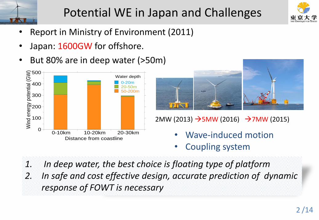
• Report in Ministry of Environment (2011)

• Japan: 1600GW for offshore.

• But 80% are in deep water (>50m)

Potential WE in Japan and Challenges

2

0

100

200

300

400

500

0-10km 10-20km 20-30km

0-20m20-50m50-200m

Win

d e

nerg

y po

ten

tial (

GW

)

Distance from coastline

Water depth

2MW (2013) 5MW (2016) 7MW (2015)

• Wave-induced motion • Coupling system

1. In deep water, the best choice is floating type of platform 2. In safe and cost effective design, accurate prediction of dynamic

response of FOWT is necessary

/14 3

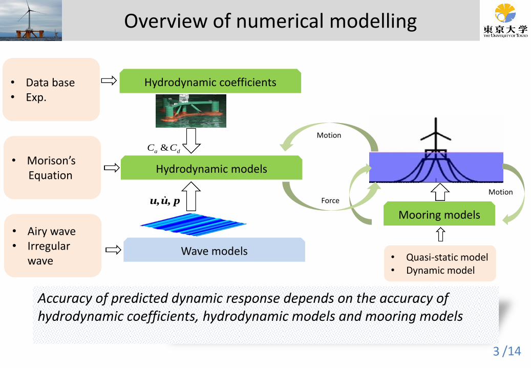
Overview of numerical modelling

&a dC C

Force

Motion

Accuracy of predicted dynamic response depends on the accuracy of hydrodynamic coefficients, hydrodynamic models and mooring models

u,u, p

• Morison’s Equation

• Airy wave • Irregular

wave

• Data base • Exp.

Hydrodynamic coefficients

Hydrodynamic models

Wave models

Mooring models

Motion

• Quasi-static model • Dynamic model

/14 4

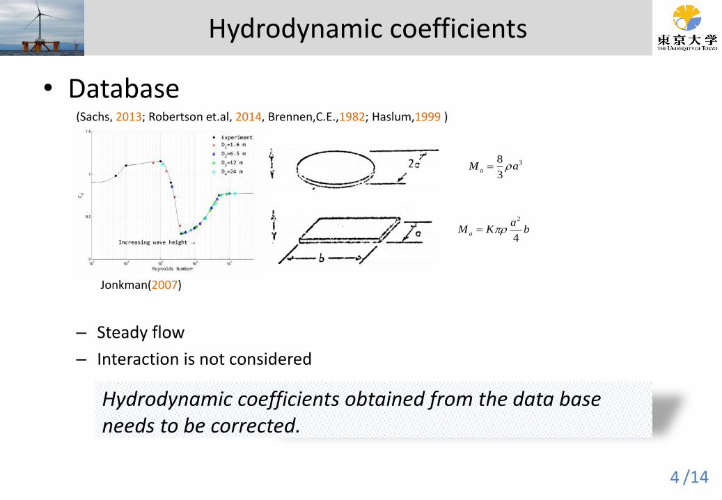
Hydrodynamic coefficients

• Database (Sachs, 2013; Robertson et.al, 2014, Brennen,C.E.,1982; Haslum,1999 )

– Steady flow

– Interaction is not considered

Hydrodynamic coefficients obtained from the data base needs to be corrected.

Jonkman(2007)

2

4a

aM K b

38

3aM a

/14 5

Hydrodynamic models

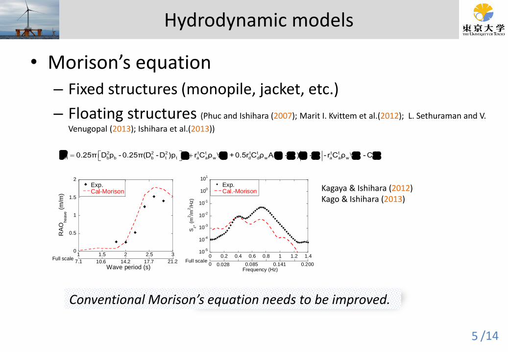
• Morison’s equation – Fixed structures (monopile, jacket, etc.)

– Floating structures (Phuc and Ishihara (2007); Marit I. Kvittem et al.(2012); L. Sethuraman and V.

Venugopal (2013); Ishihara et al.(2013))

Conventional Morison’s equation needs to be improved.

0

0.5

1

1.5

2

1 1.5 2 2.5 3

Exp.Cal-Morison

RA

Oheave (

m/m

)

Wave period (s)7.1 10.6 14.2 17.7 21.2

Full scale

Kagaya & Ishihara (2012) Kago & Ishihara (2013)

10-5

10-4

10-3

10-2

10-1

100

101

0 0.2 0.4 0.6 0.8 1 1.2 1.4

Exp.Cal.-Morison

Sz* (

m2/m

2/H

z)

Frequency (Hz)0 0.028 0.085 0.141 0.200

Full scale

F n u u x u x x xt 2 2 2 t t t t t t t t t t t t t t

H b b b t t a a w d d w a a w r0.25π D p -0.25π(D -D )p r C ρ ∀ +0.5r C ρ A( - ) - - r C ρ ∀ -C

/14 6

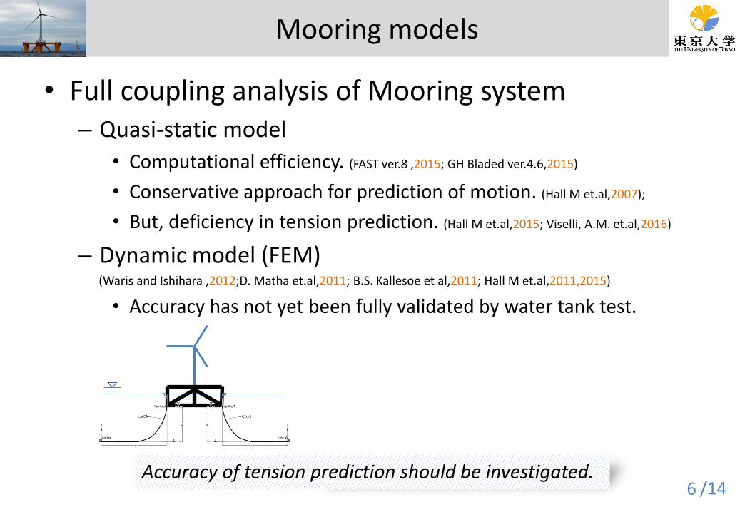
Mooring models

• Full coupling analysis of Mooring system – Quasi-static model

• Computational efficiency. (FAST ver.8 ,2015; GH Bladed ver.4.6,2015)

• Conservative approach for prediction of motion. (Hall M et.al,2007);

• But, deficiency in tension prediction. (Hall M et.al,2015; Viselli, A.M. et.al,2016)

– Dynamic model (FEM) (Waris and Ishihara ,2012;D. Matha et.al,2011; B.S. Kallesoe et al,2011; Hall M et.al,2011,2015)

• Accuracy has not yet been fully validated by water tank test.

Accuracy of tension prediction should be investigated.

/14 7

1. Propose correction factors to modify the hydrodynamic coefficients obtained from database.

2. Investigate and improve Morison’s equation to predict dynamic response of FOWT with a favorable accuracy.

3. Clarify effects of dynamic behavior of mooring system on tension prediction.

Objectives

/14 8

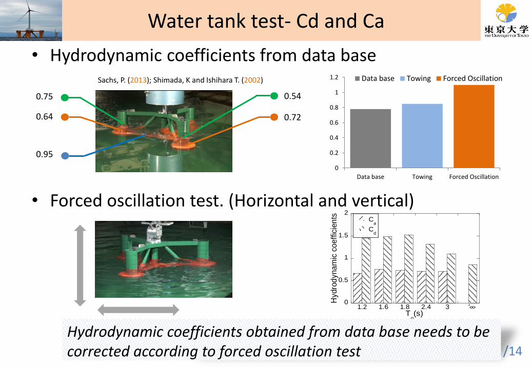
• Hydrodynamic coefficients from data base

• Forced oscillation test. (Horizontal and vertical)

0.54

0.72

0.75

0.64

0.95

Sachs, P. (2013); Shimada, K and Ishihara T. (2002)

0

0.5

1

1.5

2

1.2 1.6 1.8 2.4 3 4

Ca

Cd

Hydro

dyna

mic

co

eff

icie

nts

To(s)

Hydrodynamic coefficients obtained from data base needs to be corrected according to forced oscillation test

0

0.2

0.4

0.6

0.8

1

1.2

Data base Towing Forced Oscillation

Data base Towing

Water tank test- Cd and Ca

0

0.2

0.4

0.6

0.8

1

1.2

Data base Towing Forced Oscillation

Data base Towing Forced Oscillation

/14 9

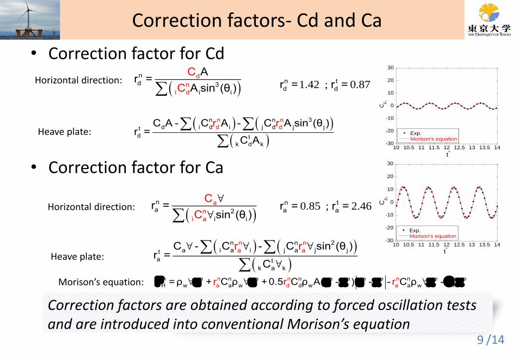
• Correction factor for Cd

• Correction factor for Ca

Correction factors- Cd and Ca

Horizontal direction:

Heave plate:

dn

d

i

n 3

i id

Ar =

A sin (θC )

C

n nn n

d d

3

d i d i j d j jt

d t

k d k

C A - C A - C A sin (θ )r =

C A

r r

1.42 ; 0.87n t

d dr = r =

an

a

i

n 2

i ia

∀r =

∀ sin (θC )

C

n nn n

a a

2

a i a i j a j jt

a t

k a k

C ∀ - C ∀ - C ∀ sin (θ )r =

C ∀

r r

Horizontal direction:

Heave plate:

0.85 ; 2.46n t

a ar = r =

-30

-20

-10

0

10

20

30

10 10.5 11 11.5 12 12.5 13 13.5 14

Exp.Morison's equation

CF

x

t*

-30

-20

-10

0

10

20

30

10 10.5 11 11.5 12 12.5 13 13.5 14

Exp.Morison's equation

CF

z

t*

F u u u x u x x C xn nn n n n n n n

a d a

n n n n n n n

H w a w d w a w r=ρ ∀ + C ρ ∀ +0.5 C ρ A( - ) - - ∀ -r C ρr rMorison’s equation:

Correction factors are obtained according to forced oscillation tests and are introduced into conventional Morison’s equation

/14 10

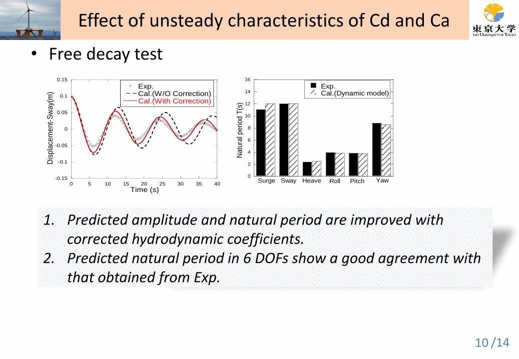
• Free decay test

Effect of unsteady characteristics of Cd and Ca

-0.15

-0.1

-0.05

0

0.05

0.1

0.15

0 5 10 15 20 25 30 35 40

Exp.Cal.(W/O Correction)

Dis

pla

cem

en

t-S

wa

y(m

)

Time (s)

0

2

4

6

8

10

12

14

16

Exp.Cal.(Dynamic model)

Natu

ral p

eriod

T(s

)

Surge HeaveSway Roll Pitch Yaw

1. Predicted amplitude and natural period are improved with corrected hydrodynamic coefficients.

2. Predicted natural period in 6 DOFs show a good agreement with that obtained from Exp.

-0.15

-0.1

-0.05

0

0.05

0.1

0.15

0 5 10 15 20 25 30 35 40

Exp.Cal.(W/O Correction)Cal.(With Correction)

Dis

pla

cem

ent-

Sw

ay(

m)

Time (s)

/14 11

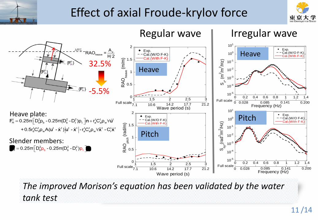
Regular wave Irregular wave

-5.5%

10-5

10-4

10-3

10-2

10-1

100

101

0 0.2 0.4 0.6 0.8 1 1.2 1.4

Exp.Cal.(W/O F-K)Cal.(With F-K)

Sy*

(ra

d2/m

2/H

z)

Frequency (Hz)0 0.028 0.085 0.141 0.200

Full scale

Pitch

The improved Morison’s equation has been validated by the water tank test

32.5%

zheave

ARAO =

H 2

0

0.5

1

1.5

2

1 1.5 2 2.5 3

Exp.Cal.(W/O F-K)

RA

Oheave

(m

/m)

Wave period (s)7.1 10.6 14.2 17.7 21.2

Full scale

0

0.5

1

1.5

2

1 1.5 2 2.5 3

Exp.Cal.(W/O F-K)Cal.(With F-K)

RA

Oheave

(m

/m)

Wave period (s)7.1 10.6 14.2 17.7 21.2

Full scale

0

0.5

1

1.5

2

1 1.5 2 2.5 3

Exp.Cal.(W/O F-K)

RA

Opitc

h (

rad/m

)

Wave period (s)

7.1 10.6 14.2 17.7 21.2Full scale

0

0.5

1

1.5

2

1 1.5 2 2.5 3

Exp.Cal.(W/O F-K)Cal.(With F-K)

RA

Opitc

h (

rad/m

)

Wave period (s)

7.1 10.6 14.2 17.7 21.2Full scale

10-5

10-4

10-3

10-2

10-1

100

101

0 0.2 0.4 0.6 0.8 1 1.2 1.4

Exp.Cal.(W/O F-K)Cal.(With F-K)

Sz*

(m

2/m

2/H

z)

Frequency (Hz)0 0.028 0.085 0.141 0.200

Full scale

Heave

Pitch

Heave

F n u

u x u x x x

t 2 2 2 t t t

H b b b t t a a w

t t t t t t t t t t t

d d w a a w r

0.25π D p -0.25π(D -D )p r C ρ ∀

+0.5r C ρ A( - ) - - r C ρ ∀ -C

Heave plate:

F nb

t 2 2 2

H b t tb0.25π D -0.25 )pπ(D -Dp

Slender members:

Effect of axial Froude-krylov force

/14 12

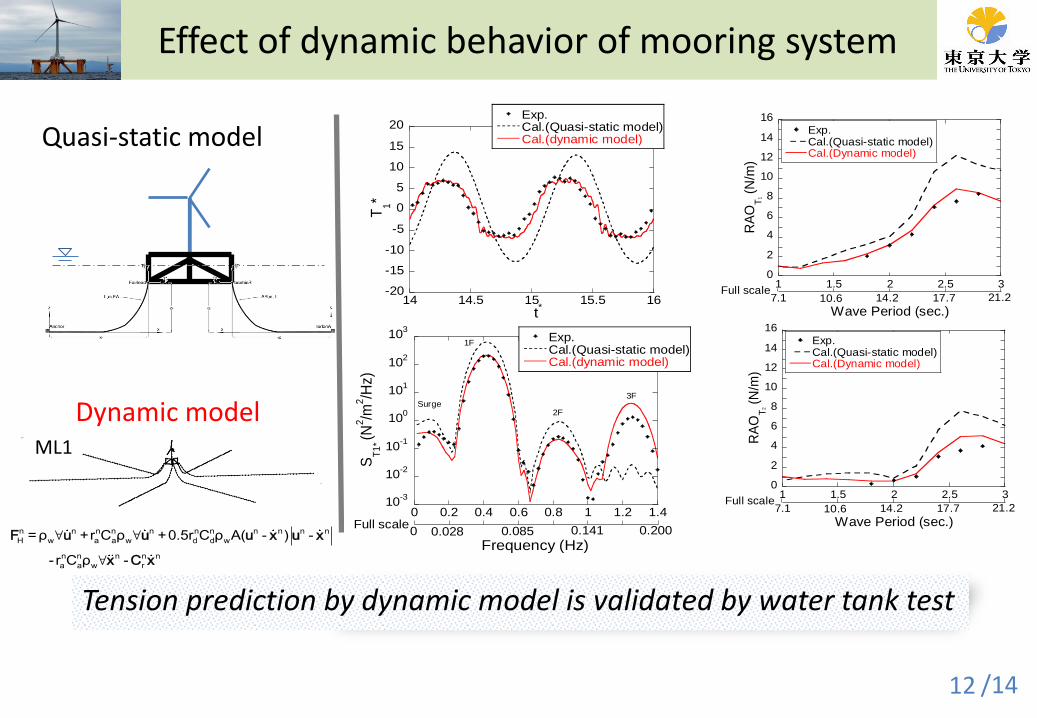
Effect of dynamic behavior of mooring system

Quasi-static model

Dynamic model ML1

0

2

4

6

8

10

12

14

16

1 1.5 2 2.5 3

Exp.Cal.(Quasi-static model)Cal.(Dynamic model)

RA

OT

1 (N

/m)

Wave Period (sec.)

Full scale7.1 10.6 14.2 17.7 21.2

Tension prediction by dynamic model is validated by water tank test

-20

-15

-10

-5

0

5

10

15

20

14 14.5 15 15.5 16

Exp.Cal.(Quasi-static model)

t*

T1*

-20

-15

-10

-5

0

5

10

15

20

14 14.5 15 15.5 16

Exp.Cal.(Quasi-static model)Cal.(dynamic model)

t*

T1*

10-3

10-2

10-1

100

101

102

103

0 0.2 0.4 0.6 0.8 1 1.2 1.4

Exp.Cal.(Quasi-static model)

Frequency (Hz)

ST

1* (N

2/m

2/H

z)

1F

2F

3FSurge

Full scale0 0.028 0.141 0.2000.085

10-3

10-2

10-1

100

101

102

103

0 0.2 0.4 0.6 0.8 1 1.2 1.4

Exp.Cal.(Quasi-static model)Cal.(dynamic model)

Frequency (Hz)

ST

1* (N

2/m

2/H

z)

1F

2F

3FSurge

Full scale0 0.028 0.141 0.2000.085

0

2

4

6

8

10

12

14

16

1 1.5 2 2.5 3

Exp.Cal.(Quasi-static model)Cal.(Dynamic model)

RA

OT

2 (N

/m)

Wave Period (sec.)

Full scale7.1 10.6 14.2 17.7 21.2

n n n n n n n n n n n

H w a a w d d w

n n n n n

a a w r

=ρ ∀ +r C ρ ∀ +0.5r C ρ A( - ) -

- r C ρ ∀ -

F u u u x u x

x C x

/14

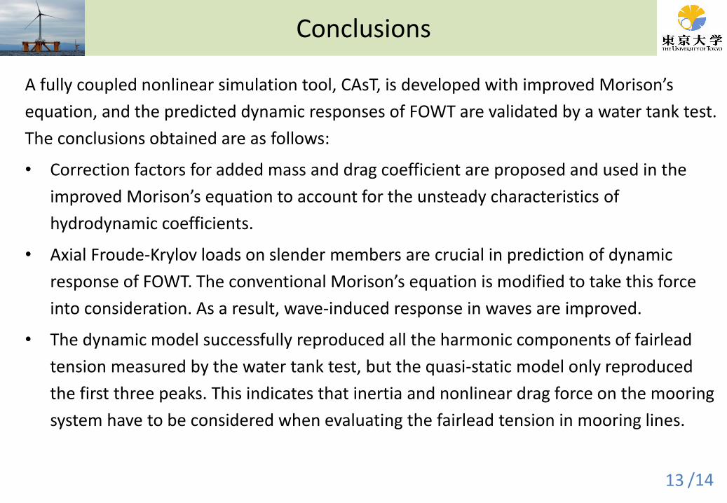
A fully coupled nonlinear simulation tool, CAsT, is developed with improved Morison’s

equation, and the predicted dynamic responses of FOWT are validated by a water tank test.

The conclusions obtained are as follows:

• Correction factors for added mass and drag coefficient are proposed and used in the

improved Morison’s equation to account for the unsteady characteristics of

hydrodynamic coefficients.

• Axial Froude-Krylov loads on slender members are crucial in prediction of dynamic

response of FOWT. The conventional Morison’s equation is modified to take this force

into consideration. As a result, wave-induced response in waves are improved.

• The dynamic model successfully reproduced all the harmonic components of fairlead

tension measured by the water tank test, but the quasi-static model only reproduced

the first three peaks. This indicates that inertia and nonlinear drag force on the mooring

system have to be considered when evaluating the fairlead tension in mooring lines.

13

Conclusions

/14 14

Thanks for your attention

Acknowledgment: This research is funded by Ministry of Economy, Trade and Industry, Japan. I wish to express my deepest gratitude to the concerned parties for their assistance and contribution in this research.