Hydrodynamic and Transport Module Short Descriptionnaturstyrelsen.dk/media/nst/65583/54335_BlueReef_ActionA2_Hyd... · DHI Software 2004 DHI Water & Environment MIKE 3/21 FLOW MODEL

DHI Software 2004

DHI Water & Environment

MIKE 3/21 FLOW MODEL FMHydrodynamic and Transport Module

Short Description

DHI Software 2004


DHI Water & EnvironmentAgern Allé 5DK-2970 HørsholmDenmark

Tel: +45 4516 9200Fax: +45 4516 9292E-mail: [email protected]: www.dhi.dk

2004-07-13/M321_FM_SHORTDESCRIPTION.DOC/OSP/HKH/MSD0407.lsm


PLEASE NOTE

COPYRIGHT This document refers to proprietary computer software,which is protected by copyright. All rights are reserved.Copying or other reproduction of this manual or the relatedprograms is prohibited without prior written consent of DHIWater & Environment (DHI). For details please refer toyour 'DHI Software Licence Agreement'.

LIMITED LIABILITY The liability of DHI is limited as specified in Section III ofyour 'DHI Software Licence Agreement':

'IN NO EVENT SHALL DHI OR ITS REPRESENTA-TIVES (AGENTS AND SUPPLIERS) BE LIABLE FORANY DAMAGES WHATSOEVER INCLUDING,WITHOUT LIMITATION, SPECIAL, INDIRECT,INCIDENTAL OR CONSEQUENTIAL DAMAGES ORDAMAGES FOR LOSS OF BUSINESS PROFITS ORSAVINGS, BUSINESS INTERRUPTION, LOSS OFBUSINESS INFORMATION OR OTHER PECUNIARYLOSS ARISING OUT OF THE USE OF OR THEINABILITY TO USE THIS DHI SOFTWARE PRODUCT,EVEN IF DHI HAS BEEN ADVISED OF THEPOSSIBILITY OF SUCH DAMAGES. THISLIMITATION SHALL APPLY TO CLAIMS OFPERSONAL INJURY TO THE EXTENT PERMITTEDBY LAW. SOME COUNTRIES OR STATES DO NOTALLOW THE EXCLUSION OR LIMITATION OFLIABILITY FOR CONSEQUENTIAL, SPECIAL,INDIRECT, INCIDENTAL DAMAGES AND,ACCORDINGLY, SOME PORTIONS OF THESELIMITATIONS MAY NOT APPLY TO YOU. BY YOUROPENING OF THIS SEALED PACKAGE ORINSTALLING OR USING THE SOFTWARE, YOUHAVE ACCEPTED THAT THE ABOVE LIMITATIONSOR THE MAXIMUM LEGALLY APPLICABLE SUBSETOF THESE LIMITATIONS APPLY TO YOURPURCHASE OF THIS SOFTWARE.'

PRINTING HISTORY July 2003............................................................Edition 2002June 2003...........................................................Edition 2003

September 2004 ................................................Edition 2004


i


CONTENTS

MIKE 3/21 FLOW MODEL FMSHORT DESCRIPTION

1 INTRODUCTION..............................................................................................1

2 GOVERNING EQUATIONS ............................................................................32.1 Shallow Water Equations........................................................................................................32.2 Transport Equations for Salt and Temperature .......................................................................42.3 Turbulence Model ...................................................................................................................4

3 NUMERICAL SOLUTION ...............................................................................73.1 Spatial Discretization ..............................................................................................................73.2 Time Integration......................................................................................................................7

4 BOUNDARY CONDITIONS............................................................................94.1 Closed Boundaries ..................................................................................................................94.2 Open Boundaries .....................................................................................................................94.3 Flooding and Drying ...............................................................................................................94.4 Resistance................................................................................................................................94.5 Wind Friction ........................................................................................................................10

5 REFERENCES.................................................................................................11

INTRODUCTION

Short Description 1


1 INTRODUCTION

The MIKE 3/21 Flow Model FM is a general hydrodynamic flowmodelling system aimed at applications within oceanographic, coastaland estuarine environments. The system comprises both two-dimensional vertically averaged equations (MIKE 21) and three-dimensional hydrostatic equations (MIKE 3).

The discretization in solution domain is performed using a finitevolume method on an unstructured mesh.

This note provides the mathematical and numerical background forMIKE 3/21 Flow Model FM1.

1 The finite volume option in MIKE 3/21 will be release in September 2004

2 MIKE 3/21 FLOW MODEL FM


GOVERNING EQUATIONS

Short Description 3


2 GOVERNING EQUATIONS

2.1 Shallow Water Equations

The model is based on the solution of the three-dimensionalincompressible Reynolds averaged Navier-Stokes equations, subject tothe assumptions of Boussinesq and of a hydrostatic pressure. Theequations are solved using a vertical σ-transformation where thetransformation ( ) /z Dσ η= −

The local continuity equation is written as

0Du Dvt x yη ω

σ∂ ∂ ∂ ∂+ + + =∂ ∂ ∂ ∂

(2.1)

and the two horizontal momentum equations for the x- and y-component, respectively

2

( / ) ( )A o T X X

Du Du Dvu ut x y

ugD p fDV A Bx x

ωσ

η ρ νσ σ

∂ ∂ ∂ ∂+ + + =∂ ∂ ∂ ∂

∂ ∂ ∂ ∂− − + + + −∂ ∂ ∂ ∂

(2.2)

2

( / ) ( )A T Y Y

Dv Duv Dv vt x y

vgD D p fDU A By y

ωσ

η ρ νσ σ

∂ ∂ ∂ ∂+ + + =∂ ∂ ∂ ∂

∂ ∂ ∂ ∂− − − + + −∂ ∂ ∂ ∂

(2.3)

whereη : elevation above mean sea level

wvu ,, : velocities in x,y,z directionsσ : vertical transformed co-ordinateD : total water depthρ : densityg : acceleration due to gravityf : Coriolis parameter

tυ : turbulent eddy viscositypA : atmospheric pressureAX,AY : horizontal stress termsBX,BY : baroclinic pressure gradients



The horizontal stress terms are described using a gradient-stressrelation, which is simplified to

( ) ( )X XY XYu uA DK DK

x x y y∂ ∂ ∂ ∂= +∂ ∂ ∂ ∂

(2.4)

and similarly for AY where KXY is an eddy viscosity.

Depth averaging of the local equations reads for the continuityequation

0=∂

∂+∂

∂+∂∂

yVH

xUH

tη

(2.5)

The transport equations for salt, temperature and turbulence are solvedafter the free surface and the velocity field.

2.2 Transport Equations for Salt and Temperature

The transports of salt or temperature follow the general transport-diffusion equations as

( )

XY XY

Z

Dc Duc Dvc ct x y

c D c c D cD Dx x x y y y

c S

ωσ

σ σσ σ

σ σ

∂ ∂ ∂ ∂+ + +∂ ∂ ∂ ∂

∂ ∂ ∂ ∂ ∂ ∂ ∂ ∂ = Γ − + Γ − ∂ ∂ ∂ ∂ ∂ ∂ ∂ ∂ ∂ ∂+ Γ +

∂ ∂

(2.6)

where c can be salinity or temperature, ΓXY and ΓZ are the diffusivityin horizontal and vertical directions and S are additional source terms,e.g. point sources, heat exchange with the atmosphere or contributionsfrom precipitation.

The temperature and salinity variations are linked to the hydrodyna-mics using an equation of state, here the UNESCO equation is used.

2.3 Turbulence Model

The turbulence is modelled assuming isotropic turbulence following agradient-stress or gradient-flux relation. Several options as constantviscosity or vertically parabolic viscosity exist, the most completebeing a standard k-ε model (Rodi, 1984), where the eddy-viscosity isderived from turbulence parameters k and ε as

GOVERNING EQUATIONS

Short Description 5


εν ν /2kCT = (2.7)

The turbulent kinetic energy k is estimated from a transport equationas

2 2( ) ( / / )kXY Z T T

Dk Duk Dvk kt x y

kA S D N D

ωσ

ν σ εσ σ

∂ ∂ ∂ ∂+ + +∂ ∂ ∂ ∂

∂ ∂= + Γ + + −∂ ∂

(2.8)

and the dissipation of TKE from

2 21 3 2( ) ( ( / / ) )XY Z T T

D Du Dvt x y

A C S D C N C Dk

εε ε ε

ε ε ε ωεσ

ε ε ν σ εσ σ

∂ ∂ ∂ ∂+ + +∂ ∂ ∂ ∂

∂ ∂= + Γ + + −∂ ∂

(2.9)

where σT is a turbulent Prandtl number, AXY are horizontal dispersionterms and S is the vertical shear, which can be written in tensornotation as

2 22 u vS

dσ σ∂ ∂ = + ∂

(2.10)

and N2 the Brunt-Vaisala frequency

2 gN ρρ σ

∂=∂

(2.11)

For the horizontal stress terms, can be used a Smagorinsky sub-gridscale eddy coefficient, which is calculated as

SlcK sXY2= (2.12)

where cs is a constant and l is the linear extent of the element.



NUMERICAL SOLUTION

Short Description 7


3 NUMERICAL SOLUTION

3.1 Spatial Discretization

The discretization in solution domain is performed using a cell-centered finite volume method. In the horizontal domain, anunstructured mesh is used. The spatial domain is discretized bysubdivision of the continuum into non-overlapping elements. Theelements can be of arbitrarily shaped polygons, however, here onlytriangles and quadrilateral elements are considered. In the verticaldomain a layered mesh is applied (see Figure 3.1). The dependentvariables of the system are represented as piecewise constants withineach element.

The convective fluxes are calculated using Roe's approximativeRiemann solver.

Figure 3.1 Principle of meshing

3.2 Time Integration

The time marching is semi-implicit using a procedure where horizontalterms are treated explicitly and vertical terms treated implicitly.



BOUNDARY CONDITIONS

Short Description 9


4 BOUNDARY CONDITIONS

4.1 Closed Boundaries

Along closed boundaries (land boundaries) normal fluxes are forced tozero for all variables. For the momentum equations this leads to full-slip along land boundaries.

4.2 Open Boundaries

The open boundary conditions can be specified either in form of a unitdischarge or as the surface elevation for the hydrodynamic equations.For transport equations either a specified value or a specified gradientcan be given.

4.3 Flooding and Drying

The approach for treatment of the moving boundaries (flooding anddrying fronts) problem is based on the work by Zhao et al. (1994) andSleigh et al. (1998). When the depths are small the problem isreformulated and only when the depths are very small the elements areremoved from the calculation. The reformulation is made by settingthe momentum fluxes to zero and only taking the mass fluxes intoconsideration.

4.4 Resistance

Several options exist for parameterization of the bed friction:

• Constant linear drag where B B BC Uτ ρ=• Quadratic drag 2

B B BC Uτ ρ=

• Chezy's formula 22z

B Bg U

Cτ =

• Manning's formula 22 4 /3B B

g UM D

ρτ =

• Bed roughness height, using the logarithmic law of the wall toderive the resistance

Here UB is the velocity in the lowermost element, CB is a dragcoefficient, CZ is the Chezy number and M is the Manning number.



4.5 Wind Friction

Drag forces from wind on the surface are related to the standard windspeed 10 m above the ground using an empirical relation

210W AIR WC Wτ ρ= (4.1)

where ρAIR is the density of air, W10 is the wind speed 10 m above theground and CW is a drag coefficient, which depends on the wind speedas

1 1

2 1 2 1 1 1 2

2 2

( ) /( )( )W

W

W

C C W WC C C W W W W W W WC C W W

= <= − − − < <= <

(4.2)

where C1, C2, W1 and W2 are empirical factors.

REFERENCES

Short Description 11


5 REFERENCES

Rodi, W. (1984), Turbulence models and their applications inhydraulics, IAHR, Delft, the Netherlands.

Sleigh, P.A., Gaskell, P.H., Bersins, M. and Wright, N.G. (1998), Anunstructured finite-volume algorithm for predicting flow in rivers andesturies, Computers & Fluids, Vol. 27, No. 4, 479-508.

Zhao, D.H., Shen, H.W., Tabios, G.Q., Tan, W.Y. and Lai, J.S. (1994),Finite-volume 2-dimensional unsteady-flow model for river basins,Journal of Hydraulic Engineering, ASCE, 1994, 120, No. 7, 863-833.



MIKE 21 & MIKE 3 FLOW MODEL FM Hydrodynamic Module

Short Description

MIKE 21 & MIKE 3 FLOW MODEL FM

Hydrodynamic Module


Agern Allé 5

DK-2970 Hørsholm

Denmark

Tel: +45 4516 9200

Fax: +45 4516 9292

E-mail: [email protected]

Web: www.dhi.dk

MIKE213_FM_Short_Descrption.doc/HKJ/AJS/BHM/MSD0602.lsm – 2006-02-10

Application Areas

MIKE 21 & MIKE 3 Flow Model FM

The Flow Model FM is a new comprehensive modelling system for two- and three-dimensional water modelling developed by DHI Water & Environment. The new 2D and 3D models carry the same names as the classic DHI model versions MIKE 21 & MIKE 3 with an ‘FM’added that refers to the type of model grid - Flexible Mesh.

The modelling system has been developed for complex applications within oceanographic, coastal and estuarine environments. However, being a general modelling system for 2D and 3D free-surface flows it may also be applied for studies of inland surface waters, e.g. overland flooding and lakes or reservoirs.

MIKE 21 & MIKE 3 Flow Model FM is a new general hydrodynamic flow modelling system based on a finite volume method on an unstructured mesh

DHI’s new Flexible Mesh (FM) series includes the following:

Flow Model FM modules: • Hydrodynamic Module, HD • Transport Module, TR • Ecology and water quality Module, ECO Lab • Sand Transport Module, ST • Mud Transport Module, MT Wave module: • Spectral Wave Module, SW

The FM Series meets the increasing demand for realistic representations of nature, both with regard to ‘look alike’ and to its capability to model coupled processes, e.g. coupling between currents,

waves and sediments. Coupling of modules is managed in the Coupled Model FM.

All modules are supported by new advanced user interfaces including efficient and sophisticated tools for mesh generation, data management, 2D/3D visualization, etc. In combination with comprehensive documentation and support, the new FM series forms a unique professional software tool for consultancy services related to design, operation and maintenance tasks within the marine environment.

An unstructured grid provides an optimal degree of flexibility in the representation of complex geometries and enables smooth representations of boundaries. Small elements may be used in areas where more detail is desired, and larger elements used where less detail is needed, optimising information for a given amount of computational time.

The spatial discretisation of the governing equations is performed using a cell-centred finite volume method. In the horizontal plane an unstructured grid is used while a structured mesh is used in the vertical domain (3D).

This document provides a short description of the Hydrodynamic Module included in MIKE 21 & MIKE 3 Flow Model FM.

Example of computational mesh for Tamar Estuary, UK

Short Description Page 1


MIKE 21 & MIKE 3 FLOW MODEL FM supports both Cartesian and spherical coordinates. Spherical coordinates are usually applied for regional and global sea circulation applications. The chart shows the computational mesh and bathymetry for the planet Earth generated by the MIKE Zero Mesh Generator

MIKE 21 & MIKE 3 Flow Model FM - Hydrodynamic Module

The Hydrodynamic Module provides the basis for computations performed in many other modules, but can also be used alone. It simulates the water level variations and flows in response to a variety of forcing functions on flood plains, in lakes, estuaries and coastal areas.

Application Areas The Hydrodynamic Module included in MIKE 21 & MIKE 3 Flow Model FM simulates unsteady flow taking into account density variations, bathymetry and external forcings.

The choice between 2D and 3D model depends on a number of factors. For example, in shallow waters, wind and tidal current are often sufficient to keep the water column well-mixed, i.e. homogeneous in salinity and temperature. In such cases a 2D model can be used. In water bodies with stratification, either by density or by species (ecology), a 3D model should be used. This is also the case for enclosed or semi-enclosed waters where wind-driven circulation occurs.

Typical application areas are

• Assessment of hydrographic conditions for design, construction and operation of structures and plants in stratified and non-stratified waters

• Environmental impact assessment studies • Coastal and oceanographic circulation studies • Optimization of port and coastal protection

infrastructures • Lake and reservoir hydrodynamics • Cooling water, recirculation and desalination • Coastal flooding and storm surge • Inland flooding and overland flow modelling • Forecast and warning systems

Example of a global tide application of MIKE 21 Flow Model FM. Results from such a model can be used as boundary conditions for regional scale forecast or hindcast models

Page 2 Hydrodynamic Module

Application Areas

The MIKE 21 & MIKE 3 Flow Model FM also support spherical coordinates, which makes both models particularly applicable for global and regional sea scale applications.

Example of a flow field in Tampa Bay, FL, simulated by MIKE 21 Flow Model FM

Study of thermal recirculation

Typical applications with the MIKE 21 & MIKE 3 Flow Model FM include cooling water recirculation and ecological impact assessment (eutrophication)

The Hydrodynamic Module is together with the Transport Module (TR) used to simulate the spreading and fate of dissolved and suspended substances. This module combination is applied in tracer simulations, flushing and simple water quality studies.

Tracer simulation of single component from outlet in the Adriatic, simulated by MIKE 21 Flow Model FM HD+TR

Prediction of ecosystem behaviour using the MIKE 21 & MIKE 3 Flow Model FM together with ECO Lab



The Hydrodynamic Module can be coupled to the Ecological Module (ECO Lab) to form the basis for environmental water quality studies comprising multiple components.

Furthermore, the Hydrodynamic Module can be coupled to sediment models for the calculation of sediment transport. The Sand Transport Module and Mud Transport Module can be applied to simulate transport of non-cohesive and cohesive sediments, respectively.

In the coastal zone the transport is mainly determined by wave conditions and associated wave-induced currents. The wave-induced currents are generated by the gradients in radiation stresses that occur in the surf zone. The Spectral Wave Module can be used to calculate the wave conditions and associated radiation stresses.

Model bathymetry of Taravao Bay, Tahiti

Coastal application (morphology) with coupled MIKE 21 HD, SW and ST, Torsminde harbour Denmark

Example of Cross reef currents in Taravao Bay, Tahiti simulated with MIKE 3 Flow Model FM. The circulation and renewal of water inside the reef is dependent on the tides, the meteorological conditions and the cross reef currents, thus the circulation model includes the effects of wave induced cross reef currents


Computational Features

Computational Features The main features and effects included in simulations with the MIKE 21 & MIKE 3 Flow Model FM – Hydrodynamic Module are the following:

• Flooding and drying • Momentum dispersion • Bottom shear stress • Coriolis force • Wind shear stress • Barometric pressure gradients • Ice coverage • Tidal potential • Precipitation/evaporation • Wave radiation stresses • Sources and sinks

Model Equations The modelling system is based on the numerical solution of the two/three-dimensional incompress-ible Reynolds averaged Navier-Stokes equations subject to the the assumptions of Boussinesq and of hydrostatic pressure. Thus, the model consists of continuity, momentum, temperature, salinity and density equations and it is closed by a turbulent closure scheme. The density does not depend on the pressure, but only on the temperature and the salinity.

For the 3D model, the free surface is taken into account using a sigma-coordinate transformation approach.

Below the governing equations are presented using Cartesian coordinates.

The local continuity equation is written as

Szw

yv

xu

=∂∂

+∂∂

+∂∂

and the two horizontal momentum equations for the x- and y-component, respectively

Suzu

zFdz

xg

xp

xgfv

zwu

yvu

xu

tu

stuza +⎟

⎠⎞

⎜⎝⎛

∂∂

∂∂

++∂∂

−∂∂

−∂∂

−=∂∂

+∂∂

+∂∂

+∂∂

∫ νρρρ

η

η

00

2

1

Svzv

zFdz

yg

yp

ygfu

zwv

xuv

yv

tv

stvza +⎟

⎠⎞

⎜⎝⎛

∂∂

∂∂

++∂∂

−∂∂

−∂∂

−−=∂∂

+∂∂

+∂∂

+∂∂

∫ νρρρ

η

η

00

2

1

Temperature and salinity In the Hydrodynamic Module, calculations of the transports of temperature, T, and salinity, s follow the general transport-diffusion equations as

STHzTD

zF

zwT

yvT

xuT

tT

svT ++⎟⎠⎞

⎜⎝⎛

∂∂

∂∂

+=∂∂

+∂∂

+∂∂

+∂∂

SszsD

zF

zws

yvs

xus

ts

svs +⎟⎠⎞

⎜⎝⎛

∂∂

∂∂

+=∂∂

+∂∂

+∂∂

+∂∂

Unstructured mesh technique gives the maximum degree of flexibility, for example: 1) Control of node distribution allows for optimal usage of nodes 2) Adoption of mesh resolution to the relevant physical scales 3) Depth-adaptive and boundary-fitted mesh. Below is shown an example from Ho Bay Denmark with the approach channel to the Port of Esbjerg



The horizontal diffusion terms are defined by

( ) ( )sTy

Dyx

Dx

FF hhsT ,, ⎥⎦

⎤⎢⎣

⎡⎟⎟⎠

⎞⎜⎜⎝

⎛∂∂

∂∂

+⎟⎠⎞

⎜⎝⎛

∂∂

∂∂

=

The equations for two-dimensional flow are obtained by integration of the equations over depth.

Heat exchange with the atmosphere is also included.


Symbol list

t time

x, y, z: Cartesian coordinates

u, v, w: flow velocity components

T, s: temperature and salinity

Dv : vertical turbulent (eddy) diffusion coefficient

H : source term due to heat exchange with atmosphere

S: magnitude of discharge due to point sources

Ts, ss : temperature and salinity of source

FT, Fs, Fc : horizontal diffusion terms

Dh : horizontal diffusion coefficient

h : depth

Solution Technique The spatial discretisation of the primitive equations is performed using a cell-centred finite volume method. The spatial domain is discretised by subdivision of the continuum into non-overlapping elements/cells.

Principle of 3D mesh

In the horizontal plane an unstructured mesh is used while a structured mesh is used in the vertical domain of the 3D model. In the 2D model the elements can be triangles or quadrilateral elements. In the 3D model the elements can be prisms or bricks whose horizontal faces are triangles and quadrilateral elements, respectively.

Model Input Input data can be divided into the following groups:

• Domain and time parameters: − computational mesh (the coordinate type is

defined in the computational mesh file) and bathymetry

− simulation length and overall time step

• Calibration factors − bed resistance − momentum dispersion coefficients − wind friction factors

• Initial conditions − water surface level − velocity components

• Boundary conditions − closed − water level − discharge

• Other driving forces − wind speed and direction − tide − source/sink discharge − wave radiation stresses

View button on all the GUIs in MIKE 21 & MIKE 3 FM HD for graphical view of input and output files

Model Input

The Mesh Generator is an efficient MIKE Zero tool for the generation and handling of unstructured meshes, including the definition and editing of boundaries

Providing MIKE 21 & MIKE 3 Flow Model FM with a suitable mesh is essential for obtaining reliable results from the models. Setting up the mesh includes the appropriate selection of the area to be modelled, adequate resolution of the bathymetry, flow, wind and wave fields under consideration and definition of codes for defining boundaries.


2D visualization of a computational mesh (Odense Estuary)

Bathymetric values for the mesh generation can e.g. be obtained from the DHI Software product MIKE C-Map. MIKE C-Map is an efficient tool for extracting depth data and predicted tidal elevation from the world-wide Electronic Chart Database CM-93 Edition 3.0 from C-Map Norway.

3D visualization of a computational mesh

If wind data is not available from an atmospheric meteorological model, the wind fields (e.g. cyclones) can be determined by using the wind-generating programs available in MIKE 21 Toolbox.

Global winds (pressure & wind data) can be downloaded for immediate use in your simulation. The sources of data are from GFS courtesy of NCEP, NOAA. By specifying the location, orientation and grid dimensions, the data is returned to you in the correct format as a spatial varying grid series or a time series. The link is: www.dhisoftware.com/mikemarine/onlinedata

The chart shows a hindcast wind field in the North Sea and Baltic Sea as wind speed and wind direction

http://www.dhisoftware.com/mikemarine/onlinedata


Model Output Computed output results at each mesh element and for each time step consist of:

• Basic variables − water depth and surface elevation − flux densities in main directions − velocities in main directions − densities, temperatures and salinities

• Additional variables − Current speed and direction − Wind velocities − Air pressure − Drag coefficient − Precipitation/evaporation − Courant/CFL number − Eddy viscosity

The output results can be saved in defined points, lines and areas. In the case of 3D calculations the results are saved in a selection of layers.

Output from MIKE 21 & MIKE 3 Flow Model FM is typically post-processed using the Data Viewer available in the common MIKE Zero shell. The Data Viewer is a tool for analysis and visualization of unstructured data, e.g. to view meshes, spectra, bathymetries, results files of different format with graphical extraction of time series and line series from plan view and import of graphical overlays.

The Data Viewer in MIKE Zero – an efficient tool for analysis and visualization of unstructured data including processing of animations. Above screen dump shows surface elevations from a model setup covering Port of Copenhagen

Vector and contour plot of current speed at a vertical profile defined along a line in Data Viewer in MIKE Zero

Validation Before the first release of MIKE 21 & MIKE 3 Flow Model FM the model was successfully applied to a number of rather basic idealized situations for which the results can be compared with analytical solutions or information from the literature.

The domain is a channel with a parabola-shaped bump in the middle. The upstream (western) boundary is a constant flux and the downstream (eastern) boundary is a constant elevation. Below: the total depths for the stationary hydraulic jump at convergence. Red line: 2D setup, green line: 3D setup, black line: analytical solution


Validation

A dam-break flow in an L-shaped channel (a, b, c):

a) Outline of model setup showing the location of gauging

points

b) Comparison between simulated and measured water

levels at the six gauge locations. (Blue) coarse mesh (black) fine mesh and (red) measurements

The model has also been applied and tested in more natural geophysical conditions; ocean scale, inner shelves, estuaries, lakes and overland, which are more realistic and complicated than academic and laboratory tests.


c) Contour plots of the surface elevation at T = 1.6 s (top)

and T = 4.8 s (bottom)

Example from Ho Bay, a tidal estuary (barrier island coast) in South-West Denmark with access channel to the Port of Esbjerg. Below: Comparison between measured and simulated water levels



The user interface of the MIKE 21 and MIKE 3 Flow Model FM (Hydrodynamic Module), including an example of the extensive Online Help system

Graphical User Interface

The MIKE 21 & MIKE 3 Flow Model FM are operated through a fully Windows integrated graphical user interface (GUI). Support is provided at each stage by an Online Help system.

The common MIKE Zero shell provides entries for common data file editors, plotting facilities and a toolbox for/utilities as the Mesh Generator and Data Viewer.

Overview of the common MIKE Zero utilities

Hardware and Operating System Requirements

Hardware and Operating System Requirements The MIKE 21 & MIKE 3 Flow Model FM are available for PCs with Microsoft Windows XP Professional Edition, Microsoft Windows 2000 and Microsoft Windows XP Professional x64 Edition. Microsoft Internet Explorer (IE) is required for network license management as well as for accessing the Online Help.

The recommended minimum hardware requirements for executing MIKE 21 & MIKE 3 Flow Model FM are:


Processor: Pentium, AMD or compatible processor; 2 GHz (or higher)

Memory (RAM): 512 MB (or higher)

Hard disk: 20 GB (or higher)

Monitor: SVGA, resolution 1024x768

Graphic card: 32 MB RAM (or higher), 24 bit true colour

CD-ROM/DVD drive: for installation of software

Support News about new features, applications, papers, updates, patches, etc. are available at the MIKE 21 Website located at:

http://www.dhisoftware.com/mike21

For further information please contact your local DHI Software agent or the Software Support Centre at DHI:

DHI Software Support Centre DHI Water & Environment Agern Allé 5 DK-2970 Hørsholm Denmark

Tel: +4545169333 Fax: +4545169292 Web: www.dhisoftware.com E-mail: [email protected]

References The MIKE 21 & MIKE 3 Flow Model FM are provided with comprehensive user guides, online help, scientific documentation, application examples and step-by-step training examples.

The MIKE 21 & MIKE 3 Flow Model FM have been, and are, extensively used in DHI consultancy services (some 50 studies in 20 different countries) and in several research projects.

Petersen, N.H., Rasch, P. “Modelling of the Asian Tsunami off the Coast of Northern Sumatra”, presented at the 3rd Asia-Pacific DHI Software Conference in Kuala Lumpur, Malaysia, 21-22 February, 2005

French, B. and Kerper, D. Salinity Control as a Mitigation Strategy for Habitat Improvement of Impacted Estuaries. 7th Annual EPA Wetlands Workshop, NJ, USA 2004.


http://www.dhisoftware.com/

mailto:[email protected]



DHI Note, “Flood Plain Modelling using unstructured Finite Volume Technique” January 2004 – download from http://www.dhisoftware.com/mike21/Download/Papers_Docs/M21FM_Floodplain.pdf

http://www.dhisoftware.com/mike21/Download/Papers_Docs/M21FM_Floodplain.pdf

http://www.dhisoftware.com/mike21/Download/Papers_Docs/M21FM_Floodplain.pdf

MIKE 21 WAVE MODELLINGMIKE 21 SW - Spectral Waves FM

Short Description

MIKE 21 WAVE MODELLING


Agern Allé 5

DK-2970 Hørsholm

Denmark

Tel: +45 4516 9200

Fax: +45 4516 9292

E-mail: [email protected]

Web: www.dhi.dk

MIKE21_SW_FM_Short_Description.doc/HKH/MSD0412.lsm - 2004-12-16

Computational Features


MIKE 21 SW - SPECTRAL WAVEMODEL FM

MIKE 21 SW is a state-of-the-art third generationspectral wind-wave model developed by DHIWater & Environment. The model simulates thegrowth, decay and transformation of wind-generated waves and swell in offshore and coastalareas.

MIKE 21 SW includes two different formulations:

• Fully spectral formulation• Directional decoupled parametric formulation

The fully spectral formulation is based on thewave action conservation equation, as described ine.g. Komen et al (1994) and Young (1999). Thedirectional decoupled parametric formulation isbased on a parameterisation of the wave actionconservation equation. The parameterisation ismade in the frequency domain by introducing thezeroth and first moment of the wave actionspectrum. The basic conservation equations areformulated in either Cartesian co-ordinates forsmall-scale applications and polar spherical co-ordinates for large-scale applications.

The fully spectral model includes the followingphysical phenomena:

• Wave growth by action of wind• Non-linear wave-wave interaction• Dissipation due to white-capping• Dissipation due to bottom friction

• Dissipation due to depth-induced wavebreaking

• Refraction and shoaling due to depthvariations

• Wave-current interaction• Effect of time-varying water depth• Effect of ice coverage on the wave field

The discretisation of the governing equation ingeographical and spectral space is performedusing cell-centred finite volume method. In thegeographical domain, an unstructured meshtechnique is used. The time integration isperformed using a fractional step approach wherea multi-sequence explicit method is applied for thepropagation of wave action.

MIKE 21 SW is a state-of-the-art numerical modelling toolfor prediction and analysis of wave climates in offshoreand coastal areas. BIOFOTO/Klaus K. Bentzen

A MIKE 21 SW forecast application in the North Sea and Baltic Sea. The chart shows a wave field (from the NSBS model)illustrated by the significant wave height in top of the computational mesh. See also www.waterforecast.com

http://www.waterforecast.com/


Page 2 MIKE 21 SW - Spectral Waves FM

Computational FeaturesThe main computational features of MIKE 21 SW- Spectral Wave Model FM are as follows:

• Fully spectral and directionally decoupledparametric formulations

• Source functions based on state-of-the-art 3rdgeneration formulations

• Instationary and quasi-stationary solutions• Optimal degree of flexibility in describing

bathymetry and ambient flow conditions usingdepth-adaptive and boundary-fittedunstructured mesh

• Coupling with hydrodynamic flow model formodelling of wave-current interaction andtime-varying water depth

• Flooding and drying in connection with time-varying water depths

• Cell-centred finite volume technique• Fractional step time-integration with an multi-

sequence explicit method for the propagation• Extensive range of model output parameters

(wave, swell, air-sea interaction parameters,radiation stress tensor, spectra, etc.)

Application AreasMIKE 21 SW is used for the assessment of waveclimates in offshore and coastal areas - in hindcastand forecast mode.

A major application area is the design of offshore,coastal and port structures where accurateassessment of wave loads is of utmost importanceto the safe and economic design of thesestructures.

Illustrations of typical application areas of DHIs MIKE 21SW Spectral Wave Model FM

Measured data are often not available duringperiods long enough to allow for the establishmentof sufficiently accurate estimates of extreme seastates. In this case, the measured data can then be

supplemented with hindcast data through thesimulation of wave conditions during historicalstorms using MIKE 21 SW.

Example of a global application of MIKE 21 SW. Theupper panel shows the bathymetry. Results from such amodel (cf. lower panel) can be used as boundaryconditions for regional scale forecast or hindcast models.See http://www.waterforecast.com for more details onregional and global modelling

MIKE 21 SW is particularly applicable forsimultaneous wave prediction and analysis onregional scale and local scale. Coarse spatial andtemporal resolution is used for the regional part ofthe mesh and a high-resolution boundary anddepth-adaptive mesh is describing the shallowwater environment at the coastline.

Example of a computational mesh used for transformationof offshore wave statistics using the directionallydecoupled parametric formulation

http://www.waterforecast.com/

Application Areas


MIKE 21 SW is also used for the calculation ofthe sediment transport, which for a large part isdetermined by wave conditions and associatedwave-induced currents. The wave-induced currentis generated by the gradients in radiation stressesthat occur in the surf zone. MIKE 21 SW can beused to calculate the wave conditions andassociated radiation stresses. The long-shorecurrents and sediment transport are then calculatedusing the flow and sediment transport modelsavailable in the MIKE 21 package. For such typeof applications, the directional decoupledparametric formulation of MIKE 21 SW is anexcellent compromise between the computationaleffort and accuracy.

Bathymetry (upper) and computational mesh (lower) usedin a MIKE 21 SW application on wave induced currents inGellen Bay, Germany

Map of significant wave height (upper), current field(middle) and vector field (lower). The flow field is simulatedby DHIs MIKE 21 Flow Model FM, which is dynamicallycoupled to MIKE 21 SW



Model EquationsIn MIKE 21 SW, the wind waves are representedby the wave action density spectrum ),( θσN . Theindependent phase parameters have been chosenas the relative (intrinsic) angular frequency, σ =2πf and the direction of wave propagation, θ. Therelation between the relative angular frequencyand the absolute angular frequency, ω, is given bythe linear dispersion relationship

Ukkdgk ⋅−== ωσ )tanh(

where g is the acceleration of gravity, d is thewater depth and U is the current velocity vectorand k is the wave number vector with magnitudek and direction θ. The action density, ),( θσN , isrelated to the energy density ),( θσE by

σEN =

Fully Spectral FormulationThe governing equation in MIKE 21 SW is thewave action balance equation formulated in eitherCartesian or spherical co-ordinates. In horizontalCartesian co-ordinates, the conservation equationfor wave action reads

σSNv

tN =⋅∇+

∂∂ )(

where ),,,( txN θσ is the action density, t is thetime, ),( yxx = is the Cartesian co-ordinates,

),,,( θσ ccccv yx= is the propagation velocity of awave group in the four-dimensional phase spacex , σ and θ. S is the source term for energybalance equation. ∇ is the four-dimensionaldifferential operator in the x , σ, θ-space. Thecharacteristic propagation speeds are given by thelinear kinematic relationships

Ukkd

kdUcdtxdcc gyx +

+=+== σ

)2sinh(21

21),(

sUkcdU

td

ddtdc gx ∂

∂⋅−

∇⋅+

∂∂

∂∂== σσ

σ

∂∂⋅+

∂∂

∂∂−==

mUk

md

dkdtdc σθ

θ1

Here, s is the space co-ordinate in wave directionθ and m is a co-ordinate perpendicular to s. x∇ isthe two-dimensional differential operator in thex -space.

Source FunctionsThe source function term, S, on the right hand sideof the wave action conservation equation is givenby

surfbotdsnlin SSSSSS ++++=

Here Sin represents the momentum transfer ofwind energy to wave generation, Snl the energytransfer due non-linear wave-wave interaction, Sdsthe dissipation of wave energy due to white-capping (deep water wave breaking), Sbot thedissipation due to bottom friction and Ssurf thedissipation of wave energy due to depth-inducedbreaking.

The default source functions Sin, Snl and Sds inMIKE 21 SW are similar to the source functionsimplemented in the WAM Cycle 4 model, seeKomen et al (1994).

The wind input is based on Janssen's (1989, 1991)quasi-linear theory of wind-wave generation,where the momentum transfer from the wind tothe sea not only depends on the wind stress, butalso the sea state itself. The non-linear energytransfer (through the resonant four-waveinteraction) is approximated by the DIA approach,Hasselmann et al (1985). The source functiondescribing the dissipation due to white-capping isbased on the theory of Hasselmann (1974) andJanssen (1989). The bottom friction dissipation ismodelled using the approach by Johnson andKofoed-Hansen (2000), which depends on thewave and sediment properties. The sourcefunction describing the bottom-induced wavebreaking is based on the well-proven approach ofBattjes and Janssen (1978) and Eldeberky andBattjes (1996).

A detailed description of the various sourcefunctions is available in Komen et al (1994) andSørensen et al (2003), which also includes thereferences listed above.

Numerical Methods


Directional Decoupled Parametric FormulationThe directionally decoupled parametricformulation is based on a parameterisation of thewave action conservation equation. FollowingHolthuijsen et al (1989), the parameterisation ismade in the frequency domain by introducing thezeroth and first moment of the wave actionspectrum as dependent variables.

A similar formulation is used in the MIKE 21NSW Near-shore Spectral Wind-Wave Model,which is one of the most popular models for wavetransformation in coastal and shallow waterenvironment. However, with MIKE 21 SW it isnot necessary to set up a number of differentorientated bathymetries to cover varying wind andwave directions.

The parameterisation leads to the followingcoupled equations

11111

00000

)()()()(

)()()()(

Tmc

ymc

xmc

tm

Tmc

ymc

xmc

tm

yx

yx

=∂

∂+

∂∂

+∂

∂+

∂∂

=∂

∂+

∂∂

+∂

∂+

∂∂

θ

θ

θ

θ

where m0 (x, y, θ) and m1 (x, y, θ) are the zerothand first moment of the action spectrum N(x, y, σ,θ), respectively. T0 (x, y, θ) and T1 (x, y, θ) aresource functions based on the action spectrum.The moments mn (x, y, θ) are defined as

ωθωωθ dyxNyxm nn ),,,(),,(

0∫∞

=

The source functions T0 and T1 take into accountthe effect of local wind generation (stationarysolution mode only) and energy dissipation due tobottom friction and wave breaking. The effects ofwave-current interaction are also included. Thesource functions for the local wind generation arederived from empirical growth relations, seeJohnson (1998) for details.

Numerical MethodsThe frequency spectrum (fully spectral modelonly) is split into a prognostic part for frequencieslower than a cut-off frequency σmax and ananalytical diagnostic tail for the high-frequencypart of the spectrum

( ) ( )m

EE−

=

maxmax ,,

σσθσθσ

where m is a constant (= 5) as proposed by Komenet al (1994).

The directional decoupled parametric formulation in MIKE21 SW is used extensively for calculation of the wavetransformation from deep-water to the shoreline and forwind-wave generation in local areas

Space DiscretisationThe discretisation in geographical and spectralspace is performed using cell-centred finitevolume method. In the geographical domain anunstructured mesh is used. The spatial domain isdiscretised by subdivision of the continuum intonon-overlapping elements. Triangle andquadrilateral shaped polygons are presentlysupported in MIKE 21 SW. The action density,N(σ,θ) is represented as a piecewise constant overthe elements and stored at the geometric centres.

In frequency space either an equidistant or a log-arithmic discretisation is used. In the directionalspace, an equidistant discretisation is used for bothtypes of models. The action density is representedas piecewise constant over the discrete intervals,∆σ and ∆θ, in the frequency and directional space.



Integrating the wave action conservation over anarea Ai, the frequency interval ∆σl and the direc-tional interval ∆θm gives

∫∫∫∫∫∫∫∫∫

Ω⋅∇=

Ω−Ω∂∂

∆∆

∆∆∆∆

ilm

ilmilm

A

AA

dddNv

dddSddNdt

θσ

θσσ

θσ

σθ

σθσθ

)(

where Ω is the integration variable defined on Ai.Using the divergence theorem and introducing theconvective flux NvF = , we obtain

( )

[ ]

[ ]l

mlimlimli

m

mlimlil

NE

ppmlpn

i

mli

SFF

FF

lFAt

N

σθ∆

σ∆

∆

θθ

σσ

,,2/1,,2/1,,

,2/1,,2/1,

1,,

,,

)()(1

)()(1

1

+−−

−−

−=

∂∂

−+

−+

=∑

where NE is the total number of edges in the cell,mlpyyxxmlpn nFnFF ,,,, )()( += is the normal flux

trough the edge p in geographical space withlength ∆lp. mliF ,2/1,)( +σ and 2/1,,)( +mliFθ is theflux through the face in the frequency anddirectional space, respectively.

The convective flux is derived using a first-orderupwinding scheme. In that

−−+= )(

21)(

21

jijinn NNccNNcF

where cn is the propagation speed normal to theelement cell face.

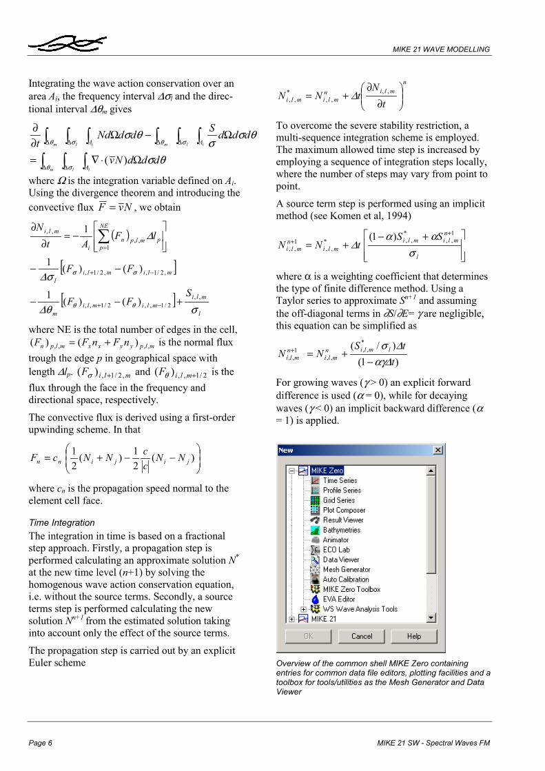
Time IntegrationThe integration in time is based on a fractionalstep approach. Firstly, a propagation step isperformed calculating an approximate solution N*

at the new time level (n+1) by solving thehomogenous wave action conservation equation,i.e. without the source terms. Secondly, a sourceterms step is performed calculating the newsolution Nn+1 from the estimated solution takinginto account only the effect of the source terms.

The propagation step is carried out by an explicitEuler scheme

nmlin

mlimli tN

tNN

∂

∂+= ,,

,,*

,, ∆

To overcome the severe stability restriction, amulti-sequence integration scheme is employed.The maximum allowed time step is increased byemploying a sequence of integration steps locally,where the number of steps may vary from point topoint.

A source term step is performed using an implicitmethod (see Komen et al, 1994)

+−+=

++

l

nmlimli

mlin

mli

SStNN

σαα

∆1,,

*,,*

,,1,,

)1(

where α is a weighting coefficient that determinesthe type of finite difference method. Using aTaylor series to approximate Sn+1 and assumingthe off-diagonal terms in ∂S/∂E= γ are negligible,this equation can be simplified as

)1()/( *

,,,,

1,, t

tSNN lmlin

mlin

mli ∆αγ∆σ

−+=+

For growing waves (γ > 0) an explicit forwarddifference is used (α = 0), while for decayingwaves (γ < 0) an implicit backward difference (α= 1) is applied.

Overview of the common shell MIKE Zero containingentries for common data file editors, plotting facilities and atoolbox for tools/utilities as the Mesh Generator and DataViewer

Model Input


Model InputThe necessary input data can be divided intofollowing groups:

• Domain and time parameters:− computational mesh− co-ordinate type (Cartesian or spherical)− simulation length and overall time step

• Equations, discretisation and solutiontechnique− formulation type− frequency and directional discretisation− number of time step groups− number of source time steps

• Forcing parameters− water level data− current data− wind data− ice data

• Source function parameters− non-linear energy transfer− wave breaking (shallow water)− bottom friction− white capping

• Initial conditions− zero-spectrum (cold-start)− empirical data− data file

• Boundary conditions− closed boundaries− open boundaries (data format and type)

Providing MIKE 21 SW with a suitable mesh isessential for obtaining reliable results from themodel. Setting up the mesh includes theappropriate selection of the area to be modelled,adequate resolution of the bathymetry, flow, windand wave fields under consideration and definitionof codes for essential and land boundaries.

Furthermore, the resolution in the geographicalspace must also be selected with respect tostability considerations.

As the wind is the main driving force in MIKE 21SW, accurate hindcast or forecast wind fields areof utmost importance for the wave prediction.

The Mesh Generator is an efficient MIKE Zero tool for thegeneration and handling of unstructured meshes, includingthe definition and editing of boundaries

3D visualisation of a computational mesh

If wind data is not available from an atmosphericmeteorological model, the wind fields (e.g.cyclones) can be determined by using the wind-generating programs available in MIKE 21Toolbox.

The chart shows an example of a wind field covering theNorth Sea and Baltic Sea as wind speed and winddirection. This is used as input to MIKE 21 SW in forecastand hindcast mode



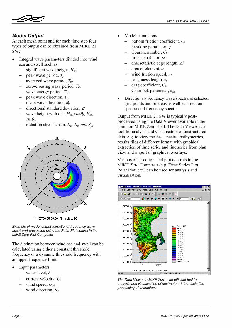
Model OutputAt each mesh point and for each time step fourtypes of output can be obtained from MIKE 21SW:

• Integral wave parameters divided into windsea and swell such as− significant wave height, Hm0− peak wave period, Tp− averaged wave period, T01− zero-crossing wave period, T02− wave energy period, T-10

− peak wave direction, θp− mean wave direction, θm

− directional standard deviation, σ− wave height with dir., Hm0 cosθm, Hm0

sinθm− radiation stress tensor, Sxx, Sxy and Syy

Example of model output (directional-frequency wavespectrum) processed using the Polar Plot control in theMIKE Zero Plot Composer

The distinction between wind-sea and swell can becalculated using either a constant thresholdfrequency or a dynamic threshold frequency withan upper frequency limit.

• Input parameters− water level, h− current velocity, U− wind speed, U10− wind direction, θw

• Model parameters− bottom friction coefficient, Cf

− breaking parameter, γ− Courant number, Cr− time step factor, α− characteristic edge length, ∆l− area of element, a− wind friction speed, u*− roughness length, z0− drag coefficient, CD− Charnock parameter, zch

• Directional-frequency wave spectra at selectedgrid points and or areas as well as directionspectra and frequency spectra

Output from MIKE 21 SW is typically post-processed using the Data Viewer available in thecommon MIKE Zero shell. The Data Viewer is atool for analysis and visualisation of unstructureddata, e.g. to view meshes, spectra, bathymetries,results files of different format with graphicalextraction of time series and line series from planview and import of graphical overlays.

Various other editors and plot controls in theMIKE Zero Composer (e.g. Time Series Plot,Polar Plot, etc.) can be used for analysis andvisualisation.

The Data Viewer in MIKE Zero an efficient tool foranalysis and visualisation of unstructured data includingprocessing of animations

Validation


ValidationThe model has successfully been applied to anumber of rather basic idealised situations forwhich the results can be compared with analyticalsolutions or information from the literature. Thebasic tests covered fundamental processes such aswave propagation, depth-induced and current-induced shoaling and refraction, wind-wavegeneration and dissipation.

Comparison between measured and simulated significantwave height, peak wave period and mean wave period atthe Ekofisk offshore platform (water depth 70 m) in theNorth Sea). () calculations and () measurements

A major application area of MIKE 21 SW is in connectionwith design and maintenance of offshore structures

The model has also been tested in naturalgeophysical conditions (e.g. in the North Sea, theDanish West Coast and the Baltic Sea), which aremore realistic and complicated than the academictest and laboratory tests mentioned above.

Comparison between measured and simulated significantwave height, peak wave period and mean wave period atFjaltring located at the Danish west coast (water depth17.5 m).() calculations and (o) measurements



The Fjaltring directional wave rider buoy is locatedoffshore relative to the depicted arrow

MIKE 21 SW is used for prediction of the waveconditions at the complex Horns Rev (reef) in thesoutheastern part of the North Sea. At this site, a168 MW offshore wind farm with 80 turbines hasbeen established in water depths between 6.5 and13.5 m.

Comparison of frequency spectra at Fjaltring. ()calculations and (-)measurements

The upper panels show the Horns Rev offshore wind farmand MIKE C-map chart. 'The middle panel shows a close-up of the mesh near the Horns Rev S wave rider buoy (t3,10 m water depth. The lower panel shows a comparisonbetween measured and simulated significant wave heightat Horns Rev S, () calculations including tide and surgeand (-) calculations excluding including tide and surge,(o) measurements

Validation


The predicted nearshore wave climate along theisland of Hiddensee and the coastline of Zingstlocated in the microtidal Gellen Bay, Germanyhave been compared to field measurements(Sørensen et al, 2004) provided by the MORWINproject. From the illustrations it can be seen thatthe wave conditions are well reproduced bothoffshore and in more shallow water near the shore.The RMS values (on significant wave height) areless than 0.25m at all five stations.

A MIKE 21 SW hindcast application in the Baltic Sea. Theupper chart shows the bathymetry and the middle andlower charts show the computational mesh. The lowerchart indicates the location of the measurement stations

Time series of significant wave height, Hm0, peak waveperiod, Tp , and mean wave direction, MWD, at Darss sill(Offshore, depth 20.5 m). () Calculation and (o)measurements. The RMS value on Hm0 is approximately0.2 m

Time series of significant wave height, Hm0, at Gellen(upper, depth 8.3m) and Bock (lower, depth 5.5 m). ()Calculation and (o) measurements. The RMS value on Hm0is approximately 0.15 m



The graphical user interface of the MIKE 21 SW model, including an example of the extensive Online Help system

Graphical User InterfaceMIKE 21 SW is operated through a fullyWindows integrated Graphical User Interface(GUI). Support is provided at each stage by anOnline Help system.

FEMA approval of the MIKE 21 package

Hardware and Operating SystemRequirementsThe module supports 2000/XP. Microsoft InternetExplorer 4.0 (or higher) is required for networklicense management as well as for accessing theOnline Help.

The recommended minimum hardwarerequirements for executing MIKE 21SW are:

Processor: Pentium, AMD orcompatible processor;2 GHz (or higher)

Memory (RAM): 512 MB (or higher)Hard disk: 20 GB (or higher)Monitor: SVGA, resolution 1024x768Graphic card: 32 MB RAM (or higher),

24 bit true colourCD-ROM/DVD drive: for installation of software

Support


SupportNews about new features, applications, papers,updates, patches, etc. are available at the MIKE 21Website located at:


For further information on MIKE 21 SW, pleasecontact your local DHI Software agent orSoftware Support Centre at DHI:

DHI Software Support CentreDHI Water & EnvironmentAgern Allé 5DK-2970 HørsholmDenmark

Tel: +4545169333Fax: +4545169292Web: www.dhisoftware.comE-mail: [email protected]

ReferencesSørensen, O. R., Kofoed-Hansen, H., Rugbjerg,M. and Sørensen, L.S., 2004: A Third GenerationSpectral Wave Model Using an UnstructuredFinite Volume Technique. In Proceedings of the29th International Conference of CoastalEngineering, 19-24 September 2004, Lisbon,Portugal.

Johnson, H.K., and Kofoed-Hansen, H., (2000).Influence of bottom friction on sea surfaceroughness and its impact on shallow water windwave modelling. J. Phys. Oceanog., 30, 1743-1756.

Johnson, H.K., Vested, H.J., Hersbach, H.Højstrup, J. and Larsen, S.E., (1999). On thecoupling between wind and waves in the WAMmodel. J. Atmos. Oceanic Technol., 16, 1780-1790.

Johnson, H.K. (1998). On modeling wind-wavesin shallow and fetch limited areas using themethod of Holthuijsen, Booij and Herbers. J.Coastal Research, 14, 3, 917-932.

Young, I.R., (1999). Wind generated ocean waves,in Elsevier Ocean Engineering Book Series,Volume 2, Eds. R. Bhattacharyya and M.E.McCormick, Elsevier.

Komen, G.J., Cavaleri, L., Doneland, M.,Hasselmann, K., Hasselmann S. and Janssen,P.A.E.M., (1994). Dynamics and modelling of

ocean waves. Cambridge University Press, UK,560 pp.

Holthuijsen, L.H, Booij, N. and Herbers, T.H.C.(1989). A prediction model for stationary, short-crested waves in shallow water with ambientcurrents, Coastal Engr., 13, 23-54.

References on ApplicationsKofoed-Hansen, H., Johnson, H.K., Højstrup, J.and Lange, B., (1998). Wind-wave modelling inwaters with restricted fetches. In: Proc of 5th

International Workshop on Wave Hindcasting andForecasting, 27-30 January 1998, Melbourne, FL,USA, pp. 113-127.

Kofoed-Hansen, H, Johnson, H.K., Astrup, P. andLarsen, J., (2001). Prediction of waves and seasurface roughness in restricted coastal waters. In:Proc of 27th International Conference of CoastalEngineering, pp.1169-1182.

Al-Mashouk, M.A., Kerper, D.R. and Jacobsen,V., (1998). Red Sea Hindcast study: Developmentof a sea state design database for the Red Sea.. JSaudi Aramco Technology, 1, 10 pp.

Rugbjerg, M., Nielsen, K., Christensen, J.H. andJacobsen, V., (2001). Wave energy in the Danishpart of the North Sea. In: Proc of 4th EuropeanWave Energy Conference, 8 pp.

MIKE 21 SW is also applied for wave forecasts in shiproute planning and improved service for conventional andfast ferry operators


http://www.dhisoftware.com/

mailto:[email protected]



Documents

Hydrodynamic and Transport Module Short Descriptionnaturstyrelsen.dk/media/nst/65583/54335_BlueReef_ActionA2_Hyd... · DHI Software 2004 DHI Water & Environment MIKE 3/21 FLOW MODEL