69    

Chapter 4

Sediment re-suspension and advection associated with residual flows in the Belgian coastal zone*

*to be submitted for publication in Journal of Marine Systems (Elsevier) M. Baeye processed and interpreted the datasets, wrote the manuscript and made all figures. N. Kumar (Coastal Processes – Sediment Dynamics lab, University of South Carolina, USA) helped in processing and interpreting the BM-ADCP datasets. V. Van Lancker and M. Fettweis are thanked for their constructive comments.

70    

Abstract Residual (e.g. wind-driven) sediment fluxes have been studied using a combination of in-situ bottom-mounted sensors (ADCP, tripod) allowing measuring over the entire water column. Flow profiles, SPM concentration and near-bed sediment dynamics are discussed, and a vertical mixing parameter is introduced in order to evaluate when suspended sediments are well-mixed in the water column. The northeast-directed flow regime exhibits strong hydrodynamics, resulting in a good mixing. Although the southwest-directed regime is also characterized by a good mixing, there is no real link with bed shear stresses (hydrodynamics). Therefore, it is suggested that the nature of particles in suspension also must be regarded. The finer, soft (cohesive) sediments are likely to be suspended more or longer compared to the more sandy sediments, which will settle more easily. These results allowed a separation and recognition of processes that control the variability of SPM concentration and that can be used as an attempt for understanding the long-term evolution of the system. Keywords: SPM Fluxes; bottom-ADCP; benthic tripod; vertical mixing

71    

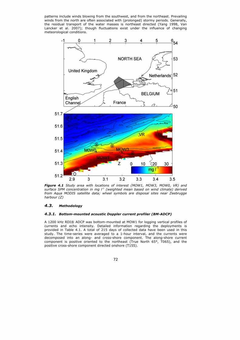
4.1. Introduction Wind stress is an important forcing mechanism for generation of flows in the inner-shelf, while in oceans, where the Coriolis acceleration dominates over other acceleration terms, geostrophic flows occur (Lentz et al. 1999, Guttierez et al. 2006, Fewings and Lentz 2009). Besides tides and density gradients, flows on the continental shelf can also be generated from bathymetric variations (Sanay et al. 2007) or from pressure gradients associated with cape-attached shoals (McNinch and Luettich 2000). Wind induced currents will change the residual transport of water masses and the residual currents (Verlaan and Groenendijk 1993, Yang 1998); they have a significant influence on the transport of particulate and dissolved substances in the water column. The importance of wind forcing on sediment transport has been discussed in various studies (e.g. Grant and Madsen 1986, Lentz 1995, Gutierrez et al. 2005). The fine-grained sediment dynamics in the southern North Sea and especially the occurrence of a turbidity maximum zone in the Belgian-Dutch coastal zone have been subject to many studies (Van Veen 1936, Nihoul 1975, Gullentops et al. 1976, Delhez and Carabin 2001, Van den Eynde 2004). The mud in the Belgian part of the North Sea partly owes its origin to the import of suspended particulate matter (SPM) from through the Dover Strait and partly to the erosion of local Holocene mud deposits (Fettweis et al. 2007, Zeelmaeckers 2011). Based on hydrodynamic data, Fettweis and Van den Eynde (2003) concluded that the decreasing residual water transport, the shallowness of the area and the difference in magnitude between neap and spring tidal currents and their effect on the erosion and transport capacity are responsible for the presence of the turbidity maximum area. The geographical variability of the turbidity maximum was investigated in Chapter 3 using satellite images and could be linked to wind forcing and direction. Measuring mean patterns of surface SPM concentration from space has become common practice (Stanev et al. 2009, Pietrzak et al. 2011). However, SPM concentration from satellite images represents a data set biased towards good weather conditions (Fettweis and Nechad 2011) and provides only near surface data. The aim of the present study is therefore to identify residual (e.g. wind-driven) sediment fluxes using in-situ bottom-mounted sensors (ADCP, tripod) that can measure over the entire water column. ADCP and multi-parametric tripods have been successfully used to measure current profiles, SPM concentration and/or near-bed sediment dynamics in shelf seas (e.g. Lynch et al. 1997, Hoitink and Hoekstra 2005). The results allow a separation and recognition of processes that control the variability of SPM concentration and can be used for understanding the long-term evolution of the system. 4.2. Study area background The measuring site MOW1 is located in the Belgian near-shore area in the vicinity of the port of Zeebrugge (Z, Fig 4.1). At this location, acoustic and optical instruments have been deployed at a water depth of about 9 m MLLWS (mean lowest low water at spring tide) (Fettweis et al. 2010, Van Lancker et al. 2007). The area is characterised by a bottom sediment composition varying from pure sand to pure mud (Verfaillie et al. 2006) and the presence of a coastal turbidity maximum (CTM) extending between Ostend (O) and the mouth of the Westerscheldt. Near-shore SPM concentration ranges between 0.02–0.07 g l–1 and reaches 0.1 to >3 g l–1 near the bed (Fettweis et al. 2010). Anthropogenic activities such as dredging and disposal influence the bed composition and the SPM concentration in the water column (Du Four and Van Lancker 2008, Lauwaert et al. 2009). The tidal regime is semi-diurnal, and the mean tidal range at Zeebrugge is 4.3 and 2.8 m at spring and neap tide, respectively. The tidal current ellipses are elongated in the near-shore area and become gradually more semi-circular towards the offshore. The current velocities near Zeebrugge (near-shore) vary from 0.2–1.5 m s–1 during spring tide and 0.2–0.6 m s–1 during neap tide. Ebb currents are directed towards the southwest and flood currents towards the northeast. The water is well mixed throughout the entire year and stratification due to salinity or temperature gradients is not occurring (de Ruijter et al. 1987). The freshwater discharge of the Westerscheldt is low (long-term annual mean is about 100 m³ s-1) and as a consequence, residual flows are mainly governed by tidal asymmetry and wind forcing (Yang 1998). Dominant wind

72    

patterns include winds blowing from the southwest, and from the northeast. Prevailing winds from the north are often associated with (prolonged) stormy periods. Generally, the residual transport of the water masses is northeast directed (Yang 1998, Van Lancker et al. 2007); though fluctuations exist under the influence of changing meteorological conditions.

Figure 4.1 Study area with locations of interest (MOW1, MOW3, MOW0, VR) and surface SPM concentration in mg l-1 (weighted mean based on wind climate) derived from Aqua MODIS satellite data; wheel symbols are disposal sites near Zeebrugge harbour (Z) 4.3. Methodology 4.3.1. Bottom-mounted acoustic Doppler current profiler (BM-ADCP) A 1200 kHz RDI® ADCP was bottom-mounted at MOW1 for logging vertical profiles of currents and echo intensity. Detailed information regarding the deployments is provided in Table 4.1. A total of 215 days of collected data have been used in this study. The time-series were averaged to a 1-hour interval, and the currents were decomposed into an along- and cross-shore component. The along-shore current component is positive oriented to the northeast (True North 65°, T065), and the positive cross-shore component directed onshore (T155).

73    

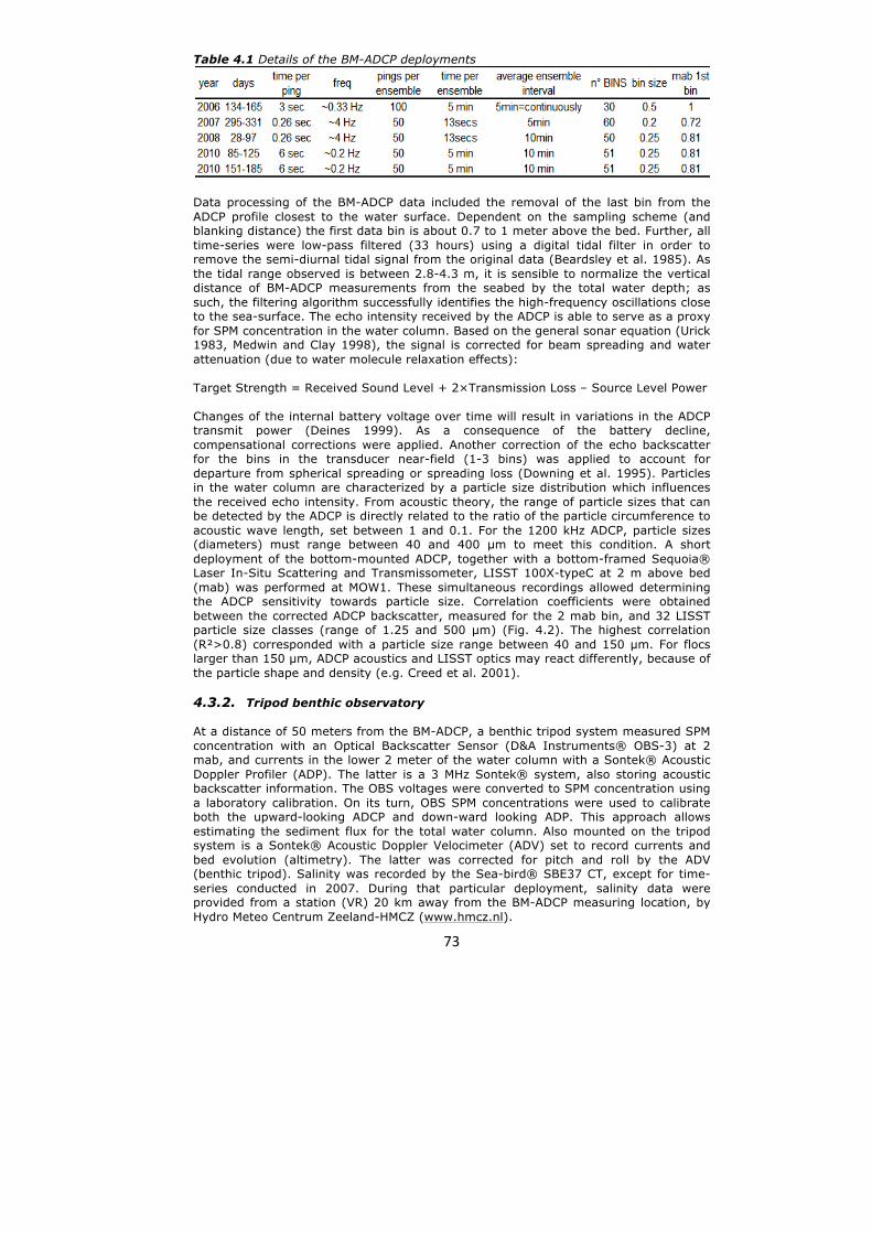
Table 4.1 Details of the BM-ADCP deployments

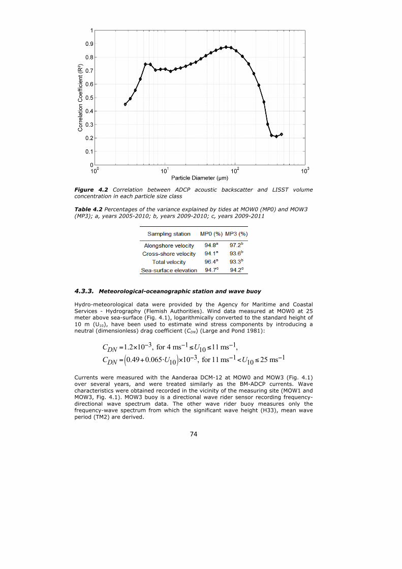
Data processing of the BM-ADCP data included the removal of the last bin from the ADCP profile closest to the water surface. Dependent on the sampling scheme (and blanking distance) the first data bin is about 0.7 to 1 meter above the bed. Further, all time-series were low-pass filtered (33 hours) using a digital tidal filter in order to remove the semi-diurnal tidal signal from the original data (Beardsley et al. 1985). As the tidal range observed is between 2.8-4.3 m, it is sensible to normalize the vertical distance of BM-ADCP measurements from the seabed by the total water depth; as such, the filtering algorithm successfully identifies the high-frequency oscillations close to the sea-surface. The echo intensity received by the ADCP is able to serve as a proxy for SPM concentration in the water column. Based on the general sonar equation (Urick 1983, Medwin and Clay 1998), the signal is corrected for beam spreading and water attenuation (due to water molecule relaxation effects): Target Strength = Received Sound Level + 2×Transmission Loss – Source Level Power Changes of the internal battery voltage over time will result in variations in the ADCP transmit power (Deines 1999). As a consequence of the battery decline, compensational corrections were applied. Another correction of the echo backscatter for the bins in the transducer near-field (1-3 bins) was applied to account for departure from spherical spreading or spreading loss (Downing et al. 1995). Particles in the water column are characterized by a particle size distribution which influences the received echo intensity. From acoustic theory, the range of particle sizes that can be detected by the ADCP is directly related to the ratio of the particle circumference to acoustic wave length, set between 1 and 0.1. For the 1200 kHz ADCP, particle sizes (diameters) must range between 40 and 400 µm to meet this condition. A short deployment of the bottom-mounted ADCP, together with a bottom-framed Sequoia® Laser In-Situ Scattering and Transmissometer, LISST 100X-typeC at 2 m above bed (mab) was performed at MOW1. These simultaneous recordings allowed determining the ADCP sensitivity towards particle size. Correlation coefficients were obtained between the corrected ADCP backscatter, measured for the 2 mab bin, and 32 LISST particle size classes (range of 1.25 and 500 µm) (Fig. 4.2). The highest correlation (R²>0.8) corresponded with a particle size range between 40 and 150 µm. For flocs larger than 150 µm, ADCP acoustics and LISST optics may react differently, because of the particle shape and density (e.g. Creed et al. 2001). 4.3.2. Tripod benthic observatory At a distance of 50 meters from the BM-ADCP, a benthic tripod system measured SPM concentration with an Optical Backscatter Sensor (D&A Instruments® OBS-3) at 2 mab, and currents in the lower 2 meter of the water column with a Sontek® Acoustic Doppler Profiler (ADP). The latter is a 3 MHz Sontek® system, also storing acoustic backscatter information. The OBS voltages were converted to SPM concentration using a laboratory calibration. On its turn, OBS SPM concentrations were used to calibrate both the upward-looking ADCP and down-ward looking ADP. This approach allows estimating the sediment flux for the total water column. Also mounted on the tripod system is a Sontek® Acoustic Doppler Velocimeter (ADV) set to record currents and bed evolution (altimetry). The latter was corrected for pitch and roll by the ADV (benthic tripod). Salinity was recorded by the Sea-bird® SBE37 CT, except for time-series conducted in 2007. During that particular deployment, salinity data were provided from a station (VR) 20 km away from the BM-ADCP measuring location, by Hydro Meteo Centrum Zeeland-HMCZ (www.hmcz.nl).

74    

Figure 4.2 Correlation between ADCP acoustic backscatter and LISST volume concentration in each particle size class Table 4.2 Percentages of the variance explained by tides at MOW0 (MP0) and MOW3 (MP3); a, years 2005-2010; b, years 2009-2010; c, years 2009-2011

4.3.3. Meteorological-oceanographic station and wave buoy Hydro-meteorological data were provided by the Agency for Maritime and Coastal Services - Hydrography (Flemish Authorities). Wind data measured at MOW0 at 25 meter above sea-surface (Fig. 4.1), logarithmically converted to the standard height of 10 m (U10), have been used to estimate wind stress components by introducing a neutral (dimensionless) drag coefficient (CDN) (Large and Pond 1981):

( )3 1 1

103 1 1

10 10

1.2 10 , for 4 ms 11 ms ,

0.49 0.065 10 , for 11 ms 25 msDN

DN

C U

C U U

− − −

− − −

= × ≤ ≤

= + ⋅ × < ≤

Currents were measured with the Aanderaa DCM-12 at MOW0 and MOW3 (Fig. 4.1) over several years, and were treated similarly as the BM-ADCP currents. Wave characteristics were obtained recorded in the vicinity of the measuring site (MOW1 and MOW3, Fig. 4.1). MOW3 buoy is a directional wave rider sensor recording frequency-directional wave spectrum data. The other wave rider buoy measures only the frequency-wave spectrum from which the significant wave height (H33), mean wave period (TM2) are derived.

75    

4.3.4. Bottom shear stress estimates BM-ADCP currents were also used for estimating bottom shear stress in the constant stress layer. This can be obtained using the law of the wall. A hydraulic bed roughness length (zo) of 0.2 mm for muddy seabeds and the ADCP first bin height (z) were used

in the following logarithmic relationship (Soulsby 1983, Wright 1989): 0* lnu zu zκ

⎛ ⎞⎜ ⎟⎜ ⎟⎝ ⎠

= ⋅ with

k, Von Karman’s constant (~0.4); u, current measured in ADCP’s first bin. Further, u*,

shear velocity is related to the current-induced bottom stress, τc, by: *2

c uτ ρ= ⋅ (ρ=1030 kg m-3 is the density of seawater). The combined shear stress was further calculated taking into account the wave oscillatory motion. Orbital velocities were obtained through solution of the linear dispersion relationship for surface gravity waves using friction factor, fw (for sediment grain size of 65 µm) in order to obtain the

wave induced shear stress: 2

8 bw

wf uρτ = ⋅

(Grasmeijer and Kleinhans 2004). The combined or total (current and waves) shear stress was calculated as follows (Nielsen

1986): ( ) ( )2 2cos sincw m w wφ φτ τ τ τ+ ⋅ + ⋅=

taking into account, Φ, the angle between wave propagation and current direction, and maximum shear stress, τm (following

Soulsby 1997):

3.21 1.2 w

m cc w

ττ τ τ τ⎡ ⎤⎛ ⎞⎢ ⎥⋅ + ⋅ ⎜ ⎟⎜ ⎟⎢ ⎥+⎝ ⎠⎢ ⎥⎣ ⎦

=.

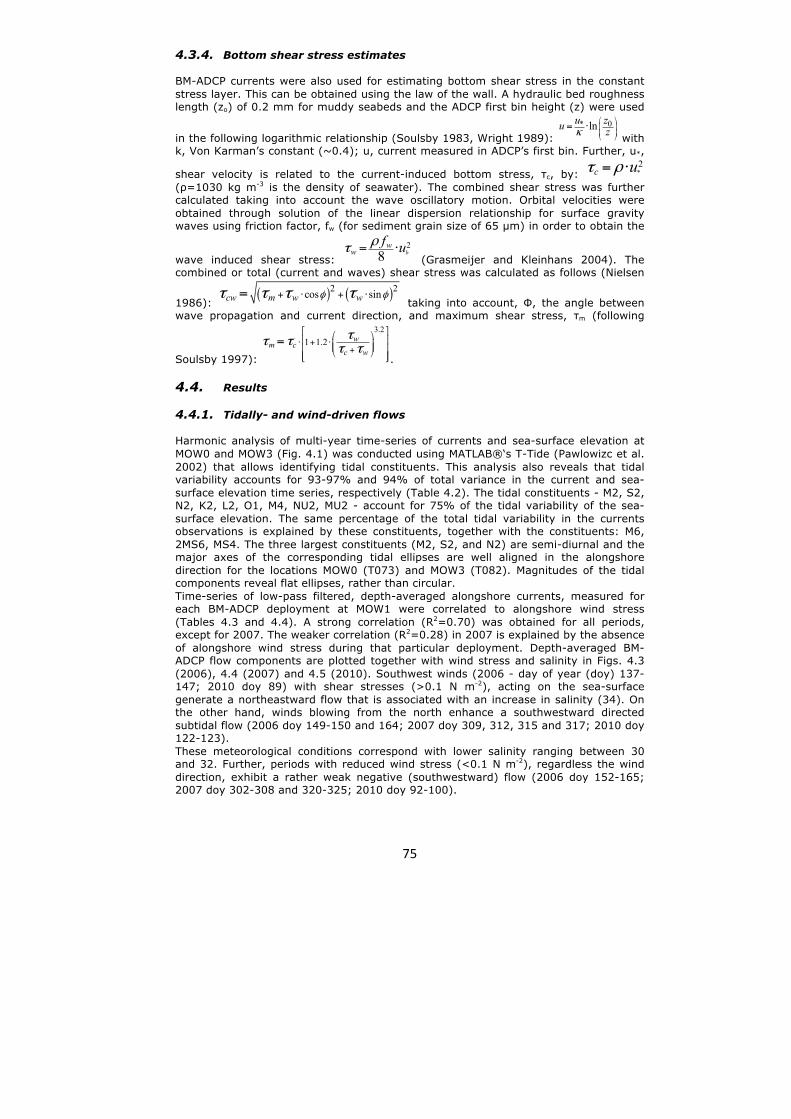
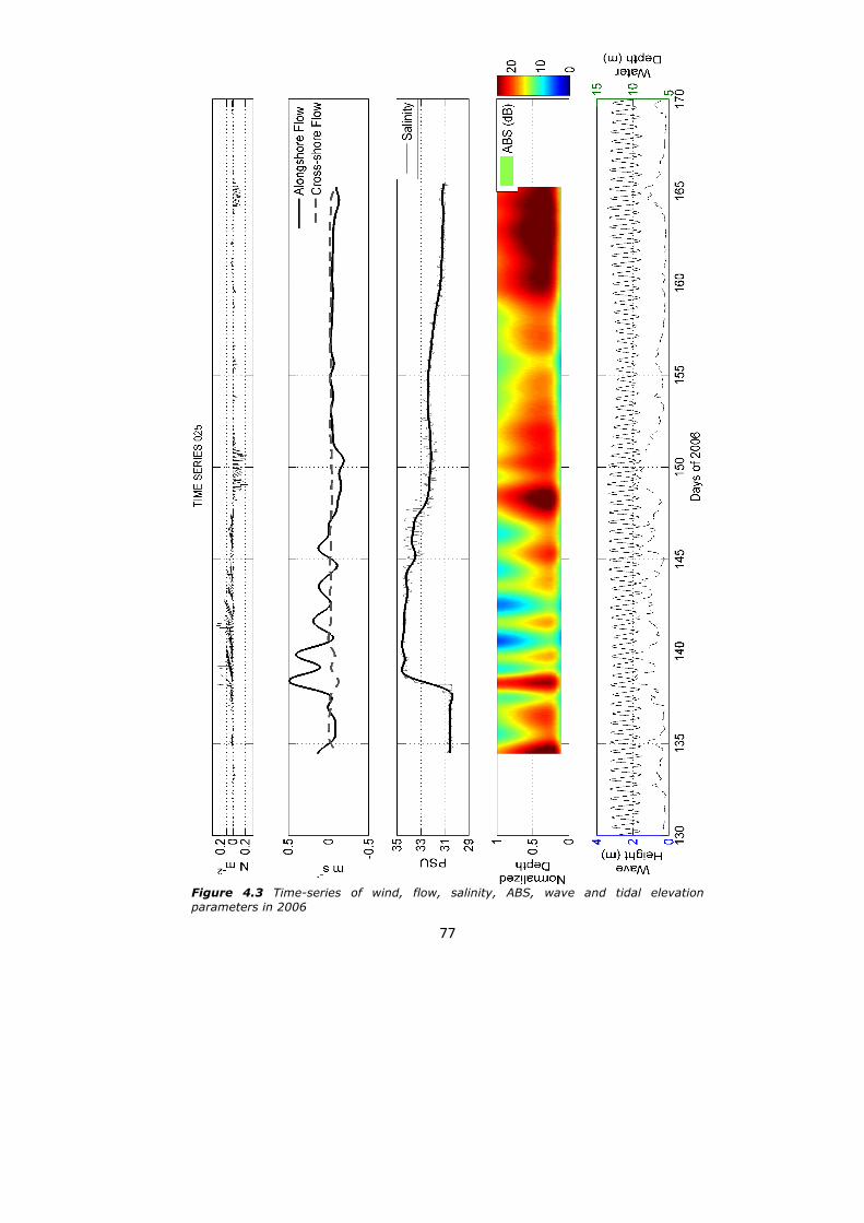
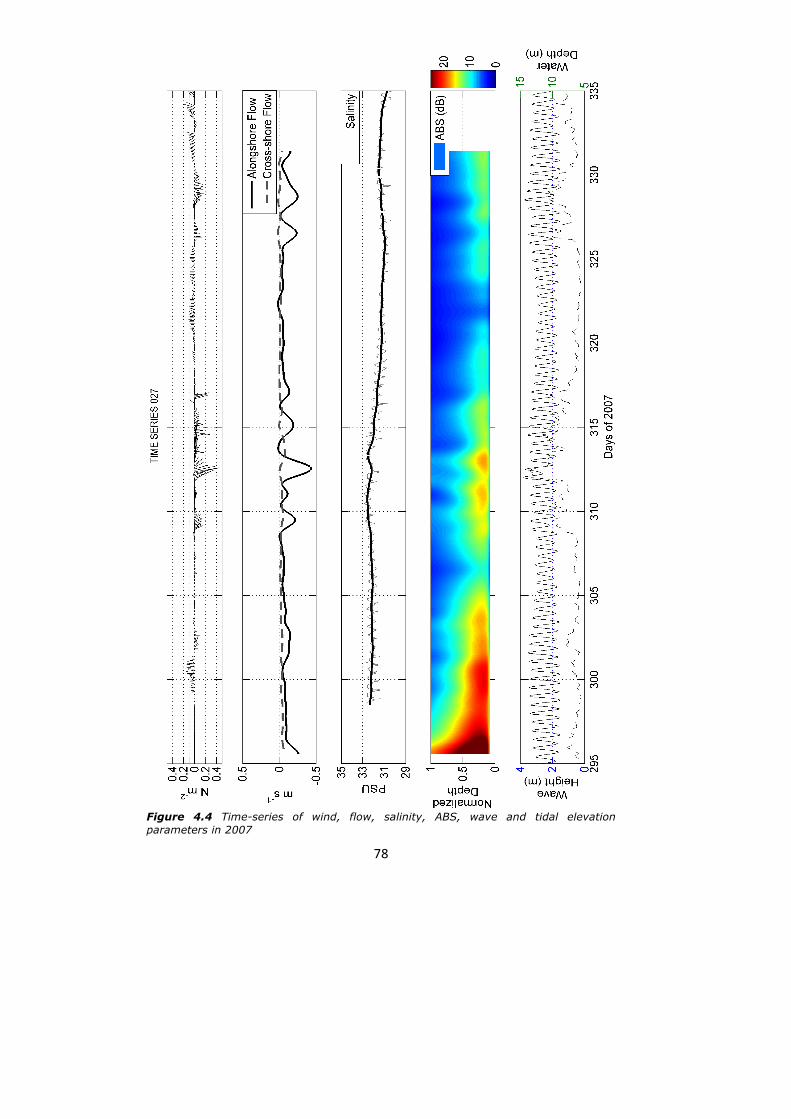
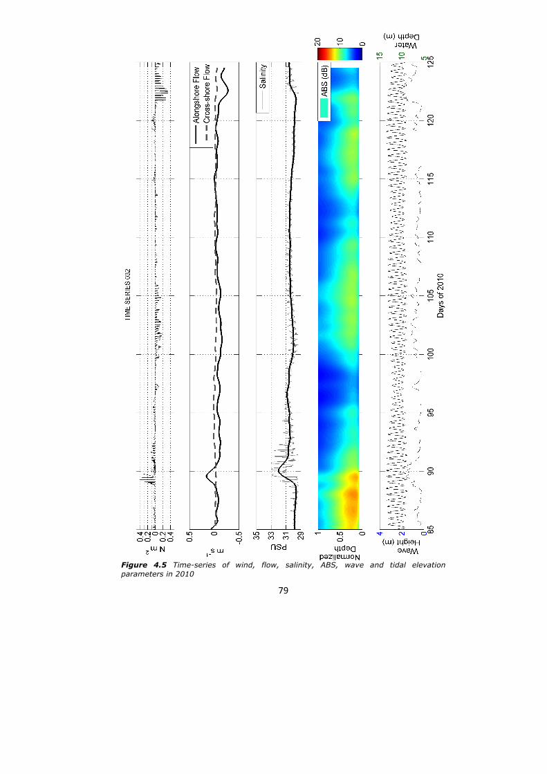
4.4. Results 4.4.1. Tidally- and wind-driven flows Harmonic analysis of multi-year time-series of currents and sea-surface elevation at MOW0 and MOW3 (Fig. 4.1) was conducted using MATLAB®‘s T-Tide (Pawlowizc et al. 2002) that allows identifying tidal constituents. This analysis also reveals that tidal variability accounts for 93-97% and 94% of total variance in the current and sea-surface elevation time series, respectively (Table 4.2). The tidal constituents - M2, S2, N2, K2, L2, O1, M4, NU2, MU2 - account for 75% of the tidal variability of the sea-surface elevation. The same percentage of the total tidal variability in the currents observations is explained by these constituents, together with the constituents: M6, 2MS6, MS4. The three largest constituents (M2, S2, and N2) are semi-diurnal and the major axes of the corresponding tidal ellipses are well aligned in the alongshore direction for the locations MOW0 (T073) and MOW3 (T082). Magnitudes of the tidal components reveal flat ellipses, rather than circular. Time-series of low-pass filtered, depth-averaged alongshore currents, measured for each BM-ADCP deployment at MOW1 were correlated to alongshore wind stress (Tables 4.3 and 4.4). A strong correlation (R2=0.70) was obtained for all periods, except for 2007. The weaker correlation (R2=0.28) in 2007 is explained by the absence of alongshore wind stress during that particular deployment. Depth-averaged BM-ADCP flow components are plotted together with wind stress and salinity in Figs. 4.3 (2006), 4.4 (2007) and 4.5 (2010). Southwest winds (2006 - day of year (doy) 137-147; 2010 doy 89) with shear stresses (>0.1 N m-2), acting on the sea-surface generate a northeastward flow that is associated with an increase in salinity (34). On the other hand, winds blowing from the north enhance a southwestward directed subtidal flow (2006 doy 149-150 and 164; 2007 doy 309, 312, 315 and 317; 2010 doy 122-123). These meteorological conditions correspond with lower salinity ranging between 30 and 32. Further, periods with reduced wind stress (<0.1 N m-2), regardless the wind direction, exhibit a rather weak negative (southwestward) flow (2006 doy 152-165; 2007 doy 302-308 and 320-325; 2010 doy 92-100).

76    

Table 4.3 Relation between wind and currents at M0W0 station, R²

Table 4.4 Relation between wind and currents for the BM-ADCP deployments, R²

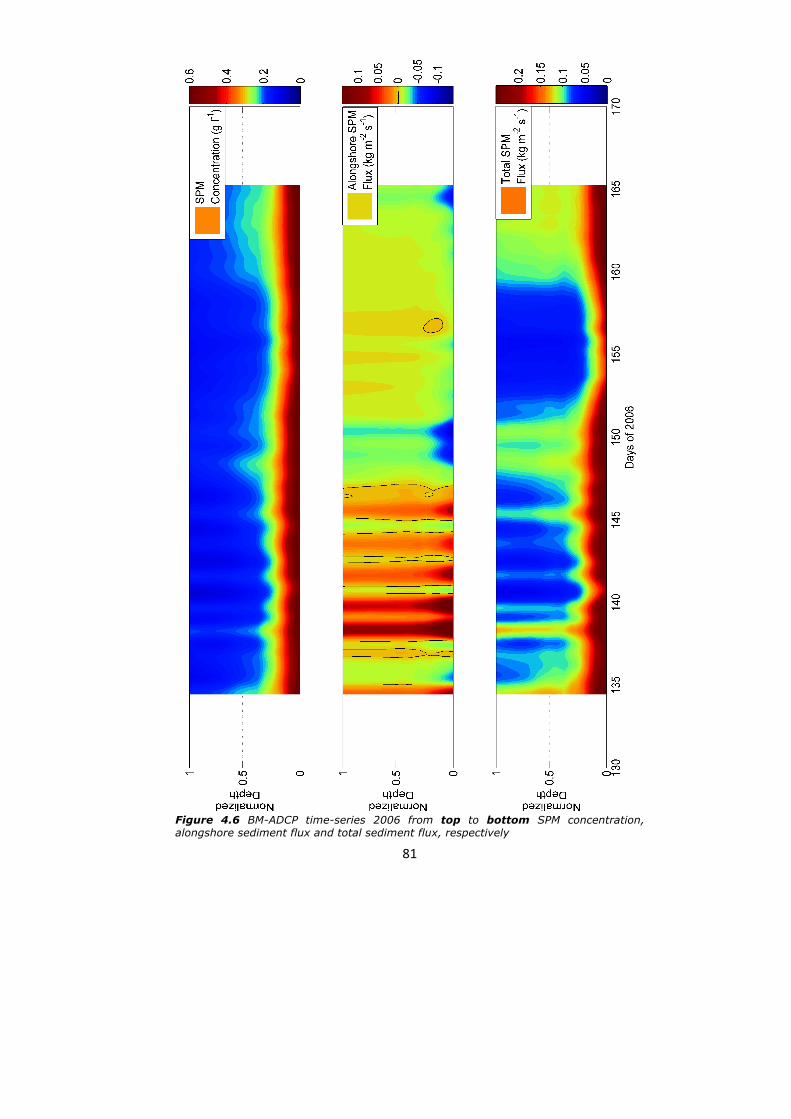
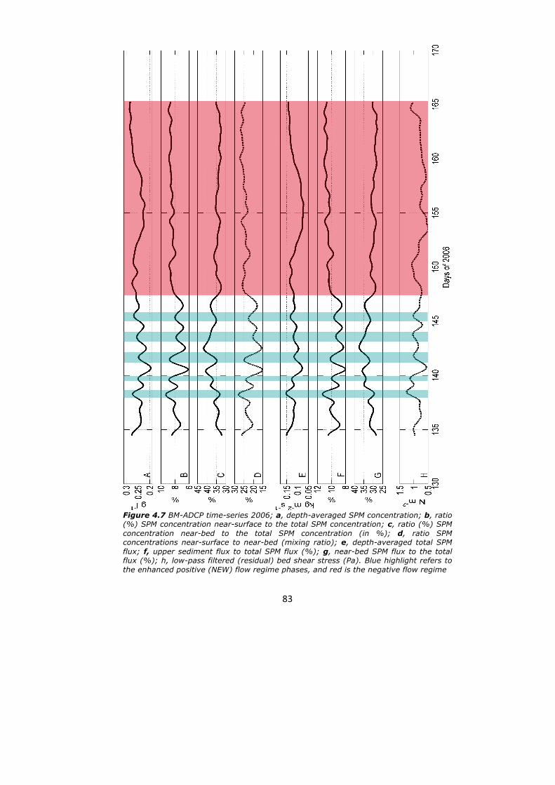
4.4.2. SPM transport (Figs. 4.3, 4.4, 4.5, 4.6) Acoustic Backscatter Signal (ABS) measured by acoustic current meters can be used as a proxy for SPM concentration. During spring tide conditions, strong tidal currents increase mixing and turbulence, leading to an increase in ABS. Superimposed on the spring-neap variation, significant meteorological events (e.g. southwesterly winds) have also an impact on the ABS due to increase of the SPM concentration. On the other hand, phases of increased ABS also exist without any relation to hydro-meteorological forcing (2006 doy 136, 157; 2010 doy 95, 111). The SPM concentration profiles derived from ADCP and ADP ABS have been combined in order to obtain profiles covering almost the entire water column (this was only done for times-series 2006) for which it was attempted to calculate the SPM fluxes (Fig. 4.6). The low-pass filtered SPM concentration exhibits low-frequency (wind-induced and spring-neap) variations. Maximum near-bed (between 0 and 1.5 mab) residual concentrations are about 0.6 g l-1. Depth-averaged SPM concentrations vary between 0.2 and 0.3 g l-1 (Fig. 4.7 a). The figures show that alongshore SPM fluxes, at that location, coincide with southwestern or northern wind events. The total SPM flux is shown in Fig. 4.7 e; one can clearly see the lower flux during neap tides (2006 doy 152-158), and the higher one (about twice) during spring tide (2006 doy 159-165). The spring-neap tidal variation in the first half (2006 doy 135-150) of the deployment is generally characterized by strong positive alongshore flows alternating with short periods of reduced or negative alongshore flow due to the prevailing meteorological conditions. Maximum depth-averaged SPM transport of 0.15 kg m-2 s-1 occurs during spring tides. On average, the lower 1.5 m of the water column accounts for 35 % of the total sediment flux (Fig. 4.7 g). 4.4.3. Wind sea waves and sediment re-suspension Wave characteristics were available during the entire time span of MODIS data image collection (about 7.5 years between 2002 and 2009; MODIS-Aqua SPM Retrieval: see Chapter 4), and each variable was assigned to each MODIS overpass (12:00-13:00 GMT) resulting in a time series of 2539 data points (i.e. number of processed MODIS SPM images). The wave population of waves travelling from the north (T315-T360 and T000-T045) and with heights >1.5m was involved for group-averaging MODIS SPM concentration maps. This resulted in a data set of 76 MODIS-SPM images. Wind direction, measured at the meteorological station MOW0, was gathered based on the time of MODIS-Aqua overpass. Waves start to become important in re-suspension of bed sediments when significant wave heights exceed 1.5 m at the measuring site (Fettweis and Nechad 2011). The increase in SPM concentration is visible along the coast, see Fig. 4.8 where the SPM concentration in the area is shown derived from

77    

Figure 4.3 Time-series of wind, flow, salinity, ABS, wave and tidal elevation parameters in 2006

78    

Figure 4.4 Time-series of wind, flow, salinity, ABS, wave and tidal elevation parameters in 2007

79    

Figure 4.5 Time-series of wind, flow, salinity, ABS, wave and tidal elevation parameters in 2010

80    

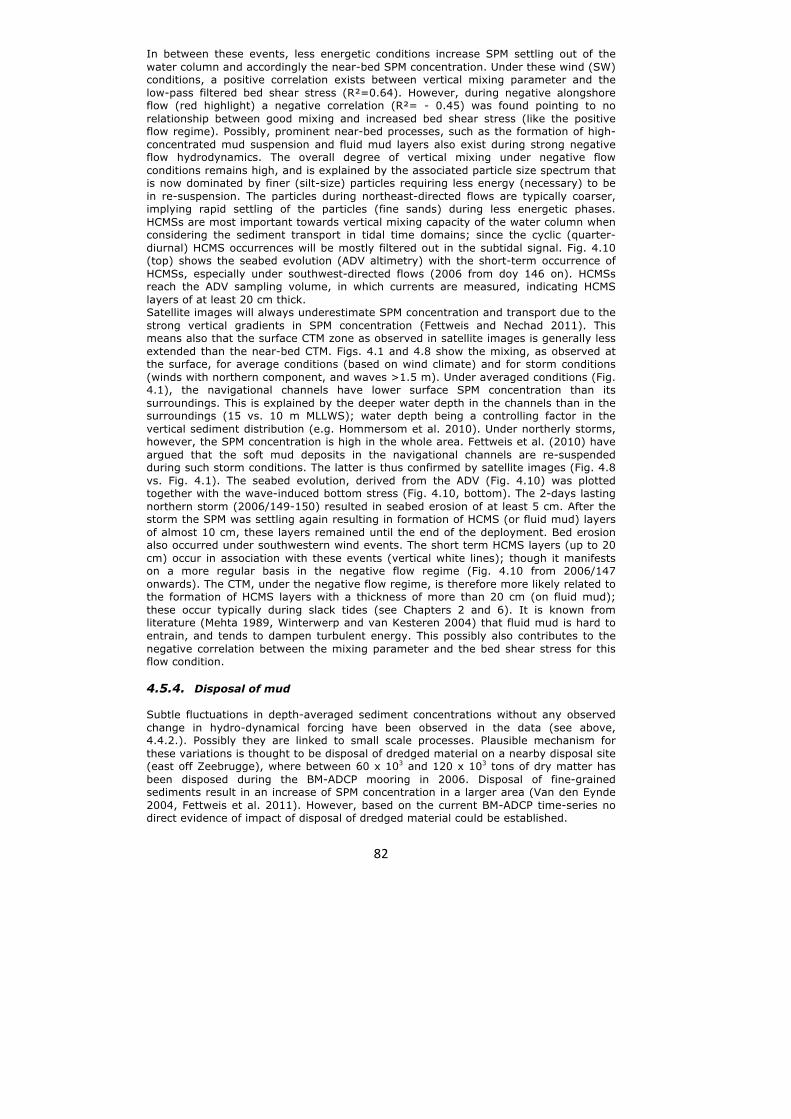
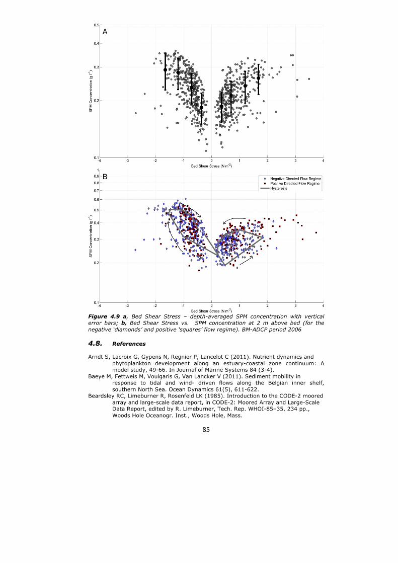
MODIS images. The coastal turbidity has an average SPM concentration at MOW1 of about 50 mg l-1, which is significantly higher than the 30 mg l-1 found in the yearly averaged image (Fig. 4.1). 4.5. Discussion 4.5.1. Subtidal flows At the measuring location (MOW1), tidal residual flows are always directed towards the southwest under weak (<0.1 N m-2) wind stress conditions. Evidence from hydrodynamic modelling shows that the measuring site is influenced by the Westerscheldt estuary, counterbalancing the northeast-directed residual transport which is generally found in the coastal zone of the southern Bight (Lacroix et al 2004, Fettweis et al. 2007). Our data confirm thus the significant influence of the Westerscheldt estuary on the hydrodynamic circulation up to at least Zeebrugge and MOW1. During weak SW wind periods, there is inertia against this circulation, directed to the SW (e.g. 2007/300-301 and 2010/119-120). However, a north-northeast wind enhances these flows. 4.5.2. Transport of sediment suspensions Bottom stress under the influence of currents and waves was computed, and correlated with depth-averaged SPM concentration from BM-ADCP deployment of 2006. SPM concentrations during the ebb are slightly higher than during flood (Fig. 4.9 a). A good correlation between bottom shear stress and SPM concentration should be expected if SPM concentration is mainly due to re-suspension by bottom shear stress. This is not the case (R²=0.50) pointing to other influencing factors such as the availability and consolidation degree of the cohesive sediments and the fluctuations in horizontal advective flux of fine sediments (e.g. Dyer 1994). In this perspective, the alongshore advection is considered (Fig. 4.9 b). Ebb coincides with higher SPM concentrations for both positive and negative subtidal flow regimes. The observed hysteresis is due to sediment entrainment and settling, and the advection of the sediment concentration gradient. The correlation between the depth-averaged, low-pass filtered SPM concentration and bed shear stress yields a good positive relationship regarding the negative flow regime (R²=0.74) since the spring-neap variation is not really overprinted by meteorological forcing, unlike the positive flow regime case (R²=0.40). Periods with stronger low-pass filtered negative flow are correlated with higher SPM concentration due to local re-suspension and advection. The tidally- and wind-driven motion of coastal waters is reflected in the salinity. Under southwest winds, the oceanic saline water is pushed through the Strait of Dover into the Belgian coastal zone. On the other hand, northern winds tend to spread out riverine, freshwater from the Scheldt-Rhine-Meuse estuaries along the Belgian coast (Yang 1998, Lacroix et al. 2004, Arndt et al. 2011). It is suggested that the negative flow will also advect sediments from the estuary towards the southwest, explaining R²=0.74. Since sediments present in the lower Scheldt are marine (Verlaan and Spanhoff 2000), an episodic buffering of sediments under prolonged periods of southwest winds was suggested (Terwindt 1977, Van Alphen 1990, Baeye et al. 2011). SPM will then subsequently be released under changing hydro-meteorological conditions (N and NE winds). In addition, the freshwater discharge (measured at 50 km upstream) was evaluated during the ADCP deployments, and continuous but low discharging (~80 m³ s-1) indicate that riverine SPM output events were not likely to be measured in the BM-ADCP time-series. 4.5.3. Vertical mixing of suspended sediments Meteorological conditions have also an influence on the vertical mixing of SPM in the water column; this depends on the settling velocities and on the vertical mixing processes (Pleskachevsky et al. 2011). Vertical mixing is calculated as the ratio between near-surface to near-bed SPM concentrations (Fig. 4.7 d). The data show that a good vertical mixing (high ratio) is associated with the major southwest wind events occurring in the first part of the 2006 time-series (blue highlights).

81    

Figure 4.6 BM-ADCP time-series 2006 from top to bottom SPM concentration, alongshore sediment flux and total sediment flux, respectively

82    

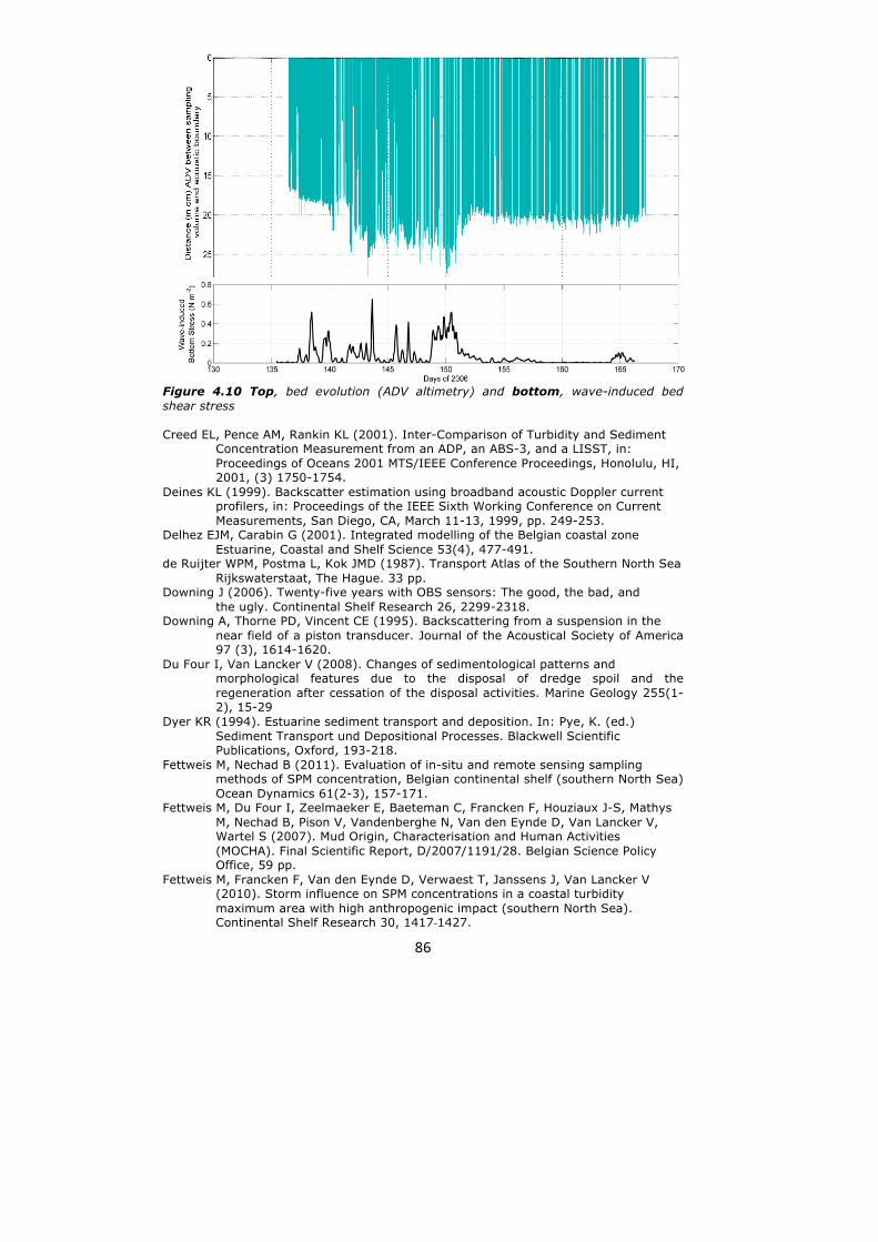
In between these events, less energetic conditions increase SPM settling out of the water column and accordingly the near-bed SPM concentration. Under these wind (SW) conditions, a positive correlation exists between vertical mixing parameter and the low-pass filtered bed shear stress (R²=0.64). However, during negative alongshore flow (red highlight) a negative correlation (R²= - 0.45) was found pointing to no relationship between good mixing and increased bed shear stress (like the positive flow regime). Possibly, prominent near-bed processes, such as the formation of high-concentrated mud suspension and fluid mud layers also exist during strong negative flow hydrodynamics. The overall degree of vertical mixing under negative flow conditions remains high, and is explained by the associated particle size spectrum that is now dominated by finer (silt-size) particles requiring less energy (necessary) to be in re-suspension. The particles during northeast-directed flows are typically coarser, implying rapid settling of the particles (fine sands) during less energetic phases. HCMSs are most important towards vertical mixing capacity of the water column when considering the sediment transport in tidal time domains; since the cyclic (quarter-diurnal) HCMS occurrences will be mostly filtered out in the subtidal signal. Fig. 4.10 (top) shows the seabed evolution (ADV altimetry) with the short-term occurrence of HCMSs, especially under southwest-directed flows (2006 from doy 146 on). HCMSs reach the ADV sampling volume, in which currents are measured, indicating HCMS layers of at least 20 cm thick. Satellite images will always underestimate SPM concentration and transport due to the strong vertical gradients in SPM concentration (Fettweis and Nechad 2011). This means also that the surface CTM zone as observed in satellite images is generally less extended than the near-bed CTM. Figs. 4.1 and 4.8 show the mixing, as observed at the surface, for average conditions (based on wind climate) and for storm conditions (winds with northern component, and waves >1.5 m). Under averaged conditions (Fig. 4.1), the navigational channels have lower surface SPM concentration than its surroundings. This is explained by the deeper water depth in the channels than in the surroundings (15 vs. 10 m MLLWS); water depth being a controlling factor in the vertical sediment distribution (e.g. Hommersom et al. 2010). Under northerly storms, however, the SPM concentration is high in the whole area. Fettweis et al. (2010) have argued that the soft mud deposits in the navigational channels are re-suspended during such storm conditions. The latter is thus confirmed by satellite images (Fig. 4.8 vs. Fig. 4.1). The seabed evolution, derived from the ADV (Fig. 4.10) was plotted together with the wave-induced bottom stress (Fig. 4.10, bottom). The 2-days lasting northern storm (2006/149-150) resulted in seabed erosion of at least 5 cm. After the storm the SPM was settling again resulting in formation of HCMS (or fluid mud) layers of almost 10 cm, these layers remained until the end of the deployment. Bed erosion also occurred under southwestern wind events. The short term HCMS layers (up to 20 cm) occur in association with these events (vertical white lines); though it manifests on a more regular basis in the negative flow regime (Fig. 4.10 from 2006/147 onwards). The CTM, under the negative flow regime, is therefore more likely related to the formation of HCMS layers with a thickness of more than 20 cm (on fluid mud); these occur typically during slack tides (see Chapters 2 and 6). It is known from literature (Mehta 1989, Winterwerp and van Kesteren 2004) that fluid mud is hard to entrain, and tends to dampen turbulent energy. This possibly also contributes to the negative correlation between the mixing parameter and the bed shear stress for this flow condition. 4.5.4. Disposal of mud Subtle fluctuations in depth-averaged sediment concentrations without any observed change in hydro-dynamical forcing have been observed in the data (see above, 4.4.2.). Possibly they are linked to small scale processes. Plausible mechanism for these variations is thought to be disposal of dredged material on a nearby disposal site (east off Zeebrugge), where between 60 x 103 and 120 x 103 tons of dry matter has been disposed during the BM-ADCP mooring in 2006. Disposal of fine-grained sediments result in an increase of SPM concentration in a larger area (Van den Eynde 2004, Fettweis et al. 2011). However, based on the current BM-ADCP time-series no direct evidence of impact of disposal of dredged material could be established.

83    

Figure 4.7 BM-ADCP time-series 2006; a, depth-averaged SPM concentration; b, ratio (%) SPM concentration near-surface to the total SPM concentration; c, ratio (%) SPM concentration near-bed to the total SPM concentration (in %); d, ratio SPM concentrations near-surface to near-bed (mixing ratio); e, depth-averaged total SPM flux; f, upper sediment flux to total SPM flux (%); g, near-bed SPM flux to the total flux (%); h, low-pass filtered (residual) bed shear stress (Pa). Blue highlight refers to the enhanced positive (NEW) flow regime phases, and red is the negative flow regime

84    

Figure 4.8 SPM concentration composite maps derived from MODIS Aqua satellite during northern storm wave conditions (winds with north component and significant wave height >1.5 m). A2 and BvH are MOW1 and MOW3, respectively. Vertical and horizontal axes are latitude and longitude (in degree), respectively 4.6. Conclusions Wind-driven flows were quantitatively investigated, and considered to be important in the study area. Time-series (40 days each) of BM-ADCP current profiles, as well as acoustic backscatter data were studied in terms of sediment transport (fluxes). An approximation of full water column SPM fluxes through combined use of ADP and BM-ADCP was realised. Based on the alongshore flow direction, two flow regimes were characterised in terms of sediment flux and vertical mixing. The negative flow regime (SWW Case; towards France) corresponds to decreased salinity and increased turbidity (higher SPM concentration). The nature of SPM is cohesive and the water column is vertical mixed; however, this mixing is not hydrodynamically controlled. Linked to this flow direction, storm waves (from the north) result in the largest extent of the coastal turbidity maximum as observed at water surface. Enhanced erosion of the seabed and mixing capacity are the main responsible mechanisms. The positive flow regime (NEW Case; towards the Netherlands) readily shows increased salinity, but decreased turbidity. This regime is characterized by vertical mixing of the water column, and high SPM fluxes. The long-term evolution of the system is therefore dependent on the mutual occurrence of the flow regimes, and thus on the wind climate. 4.7. Acknowledgements I want to acknowledge the crew of RV Belgica, Zeearend and Zeehond for their skilful mooring and recuperation of the tripod and BM-ADCP. Measurements would not have been possible without technical assistance of A. Pollentier, J-P. De Blauwe, and J. Backers (Measuring Service of MUMM, Oostende).

85    

Figure 4.9 a, Bed Shear Stress – depth-averaged SPM concentration with vertical error bars; b, Bed Shear Stress vs. SPM concentration at 2 m above bed (for the negative ‘diamonds’ and positive ‘squares’ flow regime). BM-ADCP period 2006 4.8. References Arndt S, Lacroix G, Gypens N, Regnier P, Lancelot C (2011). Nutrient dynamics and

phytoplankton development along an estuary-coastal zone continuum: A model study, 49-66. In Journal of Marine Systems 84 (3-4).

Baeye M, Fettweis M, Voulgaris G, Van Lancker V (2011). Sediment mobility in response to tidal and wind- driven flows along the Belgian inner shelf, southern North Sea. Ocean Dynamics 61(5), 611-622.

Beardsley RC, Limeburner R, Rosenfeld LK (1985). Introduction to the CODE-2 moored array and large-scale data report, in CODE-2: Moored Array and Large-Scale Data Report, edited by R. Limeburner, Tech. Rep. WHOI-85–35, 234 pp., Woods Hole Oceanogr. Inst., Woods Hole, Mass.

86    

Figure 4.10 Top, bed evolution (ADV altimetry) and bottom, wave-induced bed shear stress Creed EL, Pence AM, Rankin KL (2001). Inter-Comparison of Turbidity and Sediment

Concentration Measurement from an ADP, an ABS-3, and a LISST, in: Proceedings of Oceans 2001 MTS/IEEE Conference Proceedings, Honolulu, HI, 2001, (3) 1750-1754.

Deines KL (1999). Backscatter estimation using broadband acoustic Doppler current profilers, in: Proceedings of the IEEE Sixth Working Conference on Current Measurements, San Diego, CA, March 11-13, 1999, pp. 249-253.

Delhez EJM, Carabin G (2001). Integrated modelling of the Belgian coastal zone Estuarine, Coastal and Shelf Science 53(4), 477-491.

de Ruijter WPM, Postma L, Kok JMD (1987). Transport Atlas of the Southern North Sea Rijkswaterstaat, The Hague. 33 pp.

Downing J (2006). Twenty-five years with OBS sensors: The good, the bad, and the ugly. Continental Shelf Research 26, 2299-2318.

Downing A, Thorne PD, Vincent CE (1995). Backscattering from a suspension in the near field of a piston transducer. Journal of the Acoustical Society of America 97 (3), 1614-1620.

Du Four I, Van Lancker V (2008). Changes of sedimentological patterns and morphological features due to the disposal of dredge spoil and the regeneration after cessation of the disposal activities. Marine Geology 255(1-2), 15-29

Dyer KR (1994). Estuarine sediment transport and deposition. In: Pye, K. (ed.) Sediment Transport und Depositional Processes. Blackwell Scientific Publications, Oxford, 193-218.

Fettweis M, Nechad B (2011). Evaluation of in-situ and remote sensing sampling methods of SPM concentration, Belgian continental shelf (southern North Sea) Ocean Dynamics 61(2-3), 157-171.

Fettweis M, Du Four I, Zeelmaeker E, Baeteman C, Francken F, Houziaux J-S, Mathys M, Nechad B, Pison V, Vandenberghe N, Van den Eynde D, Van Lancker V, Wartel S (2007). Mud Origin, Characterisation and Human Activities (MOCHA). Final Scientific Report, D/2007/1191/28. Belgian Science Policy Office, 59 pp.

Fettweis M, Francken F, Van den Eynde D, Verwaest T, Janssens J, Van Lancker V (2010). Storm influence on SPM concentrations in a coastal turbidity maximum area with high anthropogenic impact (southern North Sea). Continental Shelf Research 30, 1417-­‐1427.

87    

Fettweis M, Van den Eynde D (2003). The mud deposits and the high turbidity in the Belgian-Dutch coastal zone, Southern bight of the North Sea. Continental Shelf Research, 23, 669-691.

Fewings MR, Lentz SJ (2009). A momentum budget for the inner continental shelf south of Massachusetts. Journal of Geophysical Research 115 C12.

Grasmeijer BT, Kleinhans MG (2004). Observed and predicted bed forms and their effect on suspended sand concentrations. Coastal Engineering 51, 351-371.

Gullentops F, Moens M, Ringele A, Sengier R (1976). Geologische kenmerken van de suspensie en de sedimenten. In: Nihoul, J., Gullentops, F. (Eds.), Project Zee- Projet Mer., vol. 4. Science Policy Office, Brussels, Belgium, pp. 1–137.

Gutierrez BT, Voulgaris G, Work PA (2006). Cross-shore variation of wind-driven flows on the inner shelf in Long Bay, South Carolina, United States, Journal of Geophysical Research 111, C03015.

Gutierrez BT, Voulgaris G, Thieler ER (2005). Exploring the persistence of sorted bedforms on the inner-shelf of Wrightsville Beach, North Carolina: Continental Shelf Research 25 (1), 65-99.

Grant WD, Madsen OS (1986). The Continental-Shelf Bottom Boundary Layer Annual Review of Fluid Mechanics 18, 265-305.

Hoitink AJF, Hoekstra P (2005). Observations of suspended sediment from ADCP and OBS measurements in a mud-dominated environment. Coastal Engineering 52(2), 103-118.

Hommersom A, Wernand MR, Peters S, Boer de J (2010). A review on substances and processes relevant for optical remote sensing of extremely turbid marine areas, with a focus on the Wadden Sea. Helgoland Marine Research 64(2), 75-92.

Lacroix G, Ruddick KG, Ozer J, Lancelot C (2004). Modelling the impact of the Scheldt and Rhine/Meuse plumes on the salinity distribution in Belgian waters (southern North Sea). Journal of Sea Research 52, 149-163.

Large WG, Pond S (1981). Open Ocean Momentum Flux Measurements in Moderate to Strong Winds. Journal of Physical Oceanography 11, 13.

Lauwaert B, Bekaert K, Berteloot M, De Backer A, Derweduwen J, Dujardin A, Fettweis M, Hillewaert H, Hoffman S, Hostens K, Ides S, Janssens J, Martens C, Michielsen T, Parmentier K, Van Hoey G, Verwaest T (2009). Synthesis report on the effects of dredged material disposal on the marine environment (licensing period 2008-2009). Report by BMM, ILVO, CD, aMT and WL BL/2009/01. 73 pp.

Lentz (1995). The Amazone River Plume during AMASSEDS: Subtidal current variability and the importance of wind forcing: Journal of Geophysical Research 100 C2, 2377-2390.

Lentz SJ, Guza RT, Elgar S, Feddersen F, Herbers THC (1999). Momentum balances on the North Carolina inner shelf. Journal of Geophysical Research 104, 18205–18226.

Lynch JF, Gross TF, Sherwood CR, JD Irish, Brumley BH (1997). Acoustical and optical backscatter measurements of sediment transport in the 1988-1989 STRESS experiment Continental Shelf Research 17 (4), 337-366.

Medwin H, Clay CS (1998). Fundamentals of Acoustical Oceanography, Academic Press. 712 pp.

McNinch JE, Luettich RA (2000). Physical processes around a cuspate foreland headland: implications to the evolution and long-term maintenance of a cape- associated shoal. Continental Shelf Research, 20 (17), 2367-2389.

Mehta AJ (1989). On estuarine cohesive sediment suspension behavior. Journal of Geophysical Research 94 C10, 14303-14314.

Nihoul J (1975). Effect of tidal stress on residual circulation and mud deposition in the southern Bight of the North Sea. Review of Pure and Applied Geophysics 113, 577–591.

Nielsen P (1986). Suspended sediment concentrations under waves. Coastal Engineering 10, 23–31.

Pawlowicz R, Beardsley B, Lentz S (2002). Classical tidal harmonic analysis with errors in matlab using t-tide. Computers & Geosciences 28, 929–937.

88    

Pietrzak JD, de Boer GJ, Eleveld MA (2011). Mechanisms controlling the intra-annual mesoscale variability of SST and SPM in the southern North Sea. Continental Shelf Research 31(6), 594-610.

Pleskachevsky A, Dobrynin M, Babanin A, Günther H, Stanev E (2011). Turbulent mixing due to surface waves indicated by remote sensing of suspended particulate matter and its implementation into coupled modelling of waves, turbulence, and circulation. Journal of Physical Oceanography 41, 708–724.

Sanay R, Voulgaris G, Warner JC (2007). Tidal asymmetry and residual circulation over linear sandbanks and their implication on sediment transport: A process-oriented numerical study, Journal of Geophysical Research 112, C12015 15 pp.

Stanev EV, Dobrynin M, Pleskachevsky A, Grayek S, Günther H (2009). Bed shear stress in the southern North Sea as an important driver for suspended sediment dynamics. Ocean Dynamics 59(2), 183-194.

Soulsby RL (1983). The bottom boundary layer of shelf seas. In Physical Oceanography of Coastal and Shelf Seas, ed. B. Johns, pp. 189-266. Amsterdam: Elsevier. 470 pp.

Soulsby (1997). Dynamics of Marine Sands, Thomas Telford, London, pp. 249. Terwindt JHJ (1977). Mud in the Dutch Delta area. Geologie en Mijnbouw 56 (3), 203-

210. Urick RJ (1983). Principles of underwater sound, 3rd ed. New York: McGraw-Hill 423

pp. Verlaan PAJ, Groenendijk FC (1993). Long term pressure gradients along the Belgian

and Dutch coast. MAST G8M report DGW-93.045, Rijkswaterstaat Tidal Waters Division.

Van Veen J (1936). Onderzoekingen in de Hoofden in verband met de gesteldheid der Nederlandse Kust, Nieuwe Verhandelingen van het Bataafse Genootschap voor Proefondervindelijke Wijsbegeerte te Rotterdam, 2e reeks, IIe deel, 252 pp.

Van Lancker V, Du Four I, Verfaillie E, Deleu S, Schelfaut K, Fettweis M, Van den Eynde D, Francken F, Monbaliu J, Giardino A, Portilla J, Lanckneus J, Moerkerke G, Degraer S (2007). Management, Research and Budgetting of Aggregates in Shelf Seas related to End-users (Marebasse). Belgian Science Policy: Brussels, 139 pp.

Van Alphen JS (1990). A mud balance for Belgian–Dutch coastal waters between 1969 and 1986. Netherlands Journal of Sea Research 25, 19–30.

Verfaillie E, Van Lancker V, Van Meirvenne M (2006). Multi-variate geostatistics for the predictive modelling of the surficial sand distribution in shelf seas Continental Shelf Research 26(19), 2454-2468.

Van den Eynde D (2004). Interpretation of tracer experiments with fine-grained dredging material at the Belgian Continental Shelf by the use of numerical models. Journal of Marine Systems 48, 171-189.

Verlaan PAJ, Spanhoff R (2000). Massive sedimentation events at the mouth of the Rotterdam waterway. Journal of Coastal Research 16, 458-­‐469.

Winterwerp JC, Van Kesteren WGM (2004). Introduction to the physics of cohesive sediment in the marine environment. Developments in Sedimentology 56, (Elsevier, Amsterdam). 576 pp.

Wright LD (1989). Benthic boundary layers of estuarine and coastal environments. Reviews in Aquatic Sciences 1(1), 75-95.

Yang L (1998). Modelling of hydrodynamic processes in the Belgian Coastal Zone, Applied Mathematics. Catholic University of Louvain, Leuven, pp. 204.

Zeelmaekers E (2011). Computerized qualitative and quantitative clay mineralogy: introduction and application to known geological cases. PhD Thesis. Katholieke Universiteit Leuven. Groep Wetenschap en Technologie: Heverlee. ISBN 978-90-8649-414-9. XII, 397 pp.