Huygens’ principle in electromagnetics

I.V.Lindell

Indexing terms: Huygens ’ principle, Electromagnetic theory, Transmission-line theory

I 1 Abstract: A simple way of deriving Huygens’ principle in electromagnetic and transmission- line theory is given without recourse to Green’s functions and Green’s formulas.

I I

1 Introduction

Christiaan Huygens (1629 - 1695) was a Dutch scientist who preferred the wave theory of light first proposed by Robert Hooke (1635 - 1703) to the corpuscular the- ory of Isaac Newton (1642 - 1727). Huygens imagined light analogous to sound, whose source excites motion in the particles of the surrounding medium, which transfer the motion forward. This led him to formulate what has since been known as Huygens’ principle: [ 1, 21

‘There is a further consideration in the emanation of these waves, that each particle of matter in which a wave spreads, ought not to communicate its motion only to the next particle which is in the straight line drawn from the luminous point, but that it also imparts some of it necessarily to all others which touch it and oppose themselves to its monement. So it arises that around each particle there is made a wave of which that particle is the centre.’

This principle implies that all points of a wavefront can be understood as source points creating a second- ary wavefront. In other words, the original source of the wavefront can be ignored and the wavefront itself is considered as a source for all further wavefronts.

The principle stated by Huygens was not expressed in mathematical form until Gustav Kirchhoff formulated it for scalar fields in 1882, and Stratton and Chu for vector fields in 1939 [3, 41 [Note I]. The full vector the- ory has taken a standard form in textbooks, assuming an isotropic medium and invoking the Green’s function of the medium, which, together with the derivation of Green’s integal formulas, takes quite a few pages, see, for example, [5-91. In another form, the same principle is presented as an equivalent source method, [lo-121. However, Huygens’ principle itself does not depend on Green’s functions and can be formulated very simply, as is seen below [13]. Because we do not need the Green’s function of the medium, Huygens’ principle is valid also in media for which we do not know the Green’s functions, for example anisotropic or nonlin- ear. 0 IEE, 1996 IEE Proceedings online no. 19960218 Paper first received 5th September and in revised form 4th December 1995 The author is with the Helsinki University of Technology, Electromagnet- ics Laboratory, Otakaari SA, Espoo 02150, Finland

In the present paper, Huygens’ principle is derived for the electromagnetic fields simply by truncating Maxwell’s equations. The same is done for the voltage and current in a transmission line by truncating the telegrapher’s equations. Some simple consequences are also discussed.

2 Electromagnetic field

Let us consider a closed surface S in the physical space and define one of the two regions it bounds by V. Let us further define a pulse function (or a step function) P(r) so that it has the value 1 when the vector r is in V and 0 when it is outside I/:

P(r) = 1 r E V P(r) = 0 r $ V (1) Denoting at = a/&, the electromagnetic-field problem can be defined through Maxwell‘s equations

V x E + & B = - J , (2) V x H - &D = J (3) V . B = p r n (4)

V - D = p ( 5 ) Here, we have assumed both electric and magnetic cur- rents and charges J, p and J,, pm, which may also be equivalent ones replacing some physical sources. In the conventional notation, E and H denote the electric and magnetic fields while D and B denote the electric and magnetic flux densities.

To obtain Huygens’ priciple for computing fields in V, we multiply Maxwell’s equations (eqns. 2-5) by the function P(r) and note that P(r)V F(r) = V * {P(r)F(r)} - {VP(r)} * F(r) (6) where * denotes either dot or cross product. If we adopt the notation

for an arbitrary vector function F(r) truncated to its value inside V, Maxwell’s equations become

Fv = P(r)F(r) (7)

(8)

(9)

(10)

(11)

V x E v + &Bv = -J,v + [VP] x E

V x Hv - &Dv = J v + [VP] x H

V - B v = pmv + [VP] - B

0. Dv = pv + [VP] * D These equations express Huygens’ principle: The field vectors are equal to the original ones inside V and zero outside V. The sources of these kinds of fields are the original sources truncated to the volume V plus certain Huygens’ sources, the last terms of the equations. Thus, Huygens’ sources are equivalent to the parts of the original sources left out from the region outside V. Note 1: The Stratton-Chu theory was first published in Phys. Rev., 1939, 56, p.99

IEE Proc-Sci. Meas. Technol., Vol. 143, No. 2, March 1996 103

Huygens’ sources are denoted by J,H = -[VI‘] x E

JH = [VP] x H PmH = [PPI . B P H = [VI‘] . D

(12)

(13) (14)

(15) Because V P is zero inside and outside V, Huygens’ sources are nonzero only on the surface S. In fact, V P(r) is a vector-valued surface-delta function whose direction is normal to S pointing into the region V.

There are conditions of continuity on the surface S for the Huygens’ sources. In fact, taking the divergence operation of eqn. 13, we can write V . JH = - (VP) V x H = -8, {(VP) . D} - ( V P ) . J

= -&pH - (VP) J (16) and, similarly,

These can be interpreted so that the sources of the Huygens surface currents are the normal components of the original volume currents terminating at the sur- face S plus time changes of the surface charge densities.

To see what VP(r) stands for, let us first assume that P(r) is zero outside a finite region. Taking an arbitrary function f(r) we can expand the following integral over the whole space as

V J ~ N = -&p,H - ( V P ) . J, (17)

/PP(r j l f ( r )dV =l’V[P(.)f(r)ldV - .I P(4[Vf ( r ) l f l

= - 1 Vf(r)dV = f nf(r)dS (18)

Rere, we have twice applied Gauss’s integration theo- rem to turn volume integrals to surface integrals. The second integral expression vanishes because it equals a surface integral in infinity of a function zero in infinity. The final integral is over the boundary of the pulse function, which may go into infinity as a limit. Thus, we can symbolically write

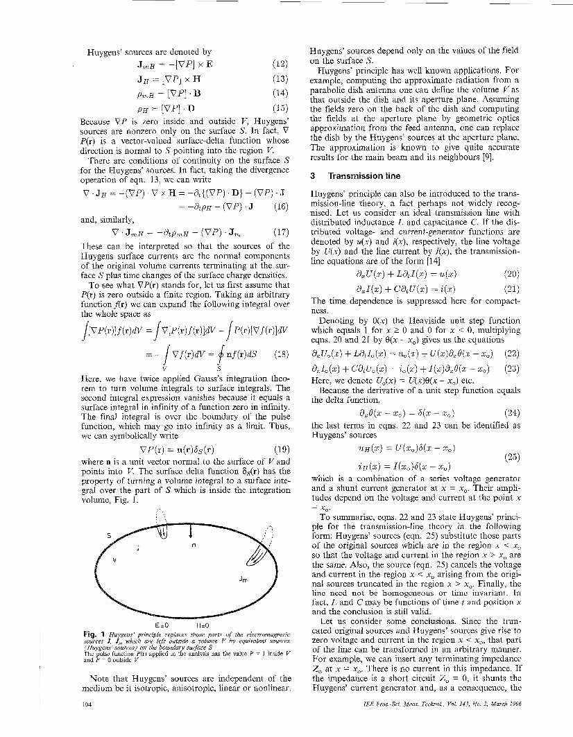
where n is a unit vector normal to the surface of V and points into V. The surface delta function 6&) has the property of turning a volume integral to a surface inte- gral over the part of S which is inside the integration volume, Fig. 1.

V S

VP(r) = n(r)ds(r) (19)

. .

E-0 H :O ig. 1 Huygens’ principle replaces those parts of the electromagnetic

sources J, J, which are left outside a volume V by equivalent sources (Huygem’ sources) on the boundary surface S The pulse functlon P(r) applied in the analysis has the value P = 1 inside V and P = 0 outside V

Note that Huygens’ sources are independent of the medium be it isotropic, anisotropic, linear or nonlinear.

Huygens’ sources depend only on the values of the field on the surface S.

Huygens’ principle has well known applications. For example, computing the approximate radiation from a parabolic dish antenna one can define the volume V as that outside the dish and its aperture plane. Assuming the fields zero on the back of the dish and computing the fields at the aperture plane by geometric optics approximation from the feed antenna, one can replace the dish by the Huygens’ sources at the aperture plane. The approximation is known to give quite accurate results for the main beam and its neighbours [9].

3 Transmission line

Huygens’ principle can also be introduced to the trans- mission-line theory, a fact perhaps not widely recog- nised. Let us consider an ideal transmission line with distributed inductance L and capacitance C. If the dis- tributed voltage- and current-generator functions are denoted by u(x) and i(x), respectively, the line voltage by U(x) and the line current by I(x), the transmission- line equations are of the form [14]

a,u(xc> + LaJ(5) = U(..)

a,I(z) + C&U(X) = i ( 2 ) (20)

(21) The time dependence is suppressed here for compact- ness.

Denoting by 8(x) the Heaviside unit step function which equals 1 for x 2 0 and 0 for x < 0, multiplying eqns. 20 and 21 by 8(x - x,) gives us the equations

a,u,(2) + La,Io(2) = U,(Z) + U(Z)d,O(Z - z,) (22)

&I,(X) + C&UO(z) = io(.) + I ( z ) d z Q ( ~ - ~ 0 ) (23)

Because the derivative of a unit step function equals Here, we denote U,(x) = U(x)e(x - x,) etc.

the delta function,

the last terms in eqns. 22 and 23 can be identified as Huygens’ sources

d,8(2 - z,) = 6 ( 2 - 2,) (24)

( 2 5 ) \- I

i H ( 2 ) = I(Zo)6(Z - 20)

which is a combination of a series voltage generator and a shunt current generator at x = x,. Their ampli- tudes depend on the voltage and current at the point x - x,.

To summarise, eqns. 22 and 23 state Huygens’ princi- ple for the transmission-line theory in the following form: Huygens’ sources (eqn. 25) substitute those parts of the original sources which are in the region x i x, so that the voltage and current in the region x > x, are the same. Also, the sowce (eqn. 25) cancels the voltage and current in the region x < x, arising from the origi- nal sources truncated in the region x > x,. Finally, the line need not be homogeneous or time invariant In fact, L and C may be functions of time t and position x and the conclusion is still valid.

Let us consider some conclusions. Since the trun- cated original sources and Wuygens’ sources give rise to zero voltage and current in the region x < xor that part of the line can be transformed in an arbitrary manner. For example, we can insert any terminating impedance Z, at x = x,. There is no current in this impedance. If the impedance is a short circuit Z, = 0, it shunts the Huygens’ current generator and, as a consequence, the

-

104 IEE Proc -Sei Meus Technol, Vol. 143, No 2, Mmch 1996

two Huygens’ sources can be replaced by the voltage source alone and a short circuit without changing the voltage and current in the section x 55 x,. Further, this arrangement can be replaced by replacing the short cir- cuit by an extension of the line to - and adding the negative image of the voltage generator, which equals the original voltage generator. Because these two gener- ators are at the same point x = 0, they can be added to a generator of double the original voltage giving the original same voltages and currents in x > x,. In this case, the voltage and current in the section x < x, are no longer zero but negative images of those in the sec- tion x > x,.

4 Time-dependent electromagnetics

The same principle can be extended to electromagnetic field problems where the Huygens’ sources are not sta- tionary. In this case, the pulse function P is a function of both space and time. For example, if the boundary of a region is moving in space with the velocity v, we may write

Proceeding as before, we obtain the Huygens’ sources P(r, t ) = P(r - vt) (26)

J H = [VP] x H - [&P]D (27)

J,H = -[VP] x E - [&P]B (28)

P H = [VP] . D (29)

P m H = [VPJ * B (30) The vector Huygens’ sources are seen to include vol- ume sources as well, because the last terms of eqns. 27 and 28 are nonzero in the volume of the pulse function P(r, t), unless d,P = 0.

As an example, let us consider moving Huygens’ sources on a transmission line by considering the unit step function of the form O(x - vt). In this case, the Huygens’ sources are U f f ( 2 ) t ) = azo(, - wt)U(z, t ) + L&d(x - wt)l(z, t )

= S(z - vt){U(z, t ) - -21Ll(z, t ) }

= S(z - ut){& t ) - vCU(z, t ) }

(31)

(32)

i H ( 2 , t ) zr &d(z - Vt) l (x , t ) + c&d(z - vt)U(z, t )

If the original point source at x = 0 is turned on at t = 0, the corresponding voltage and current functions are of the form

U0 I(z,t) = - f (z - et) (33) CL U ( z , t ) = U o f ( z - et)

where c = l/d(LC) is the velocity of the signal on the line andf(x - ct) is zero for x > ct from causality. In this case, Huygens’ sources are

(35) e-v

i H ( Z ) t ) = S(x - ut)-U,f(s - ct) c2 L

It is seen that, for v > c, these sources are zero. The reason is that they move ahead of the wave. In the region x > vt there is no signal at all. For v < c there is the region vt < x < ct of nonzero voltage and current produced by the Huygens’ sources eqns. 34 and 35, while in the region x < vt the voltage and current are zero.

Another interesting special case is obtained when the pulse function P(r, t ) depends on time only: P(t) = 1 tl < t < tl P ( t ) = 0 otherwise (36) In this case we obtain fields and sources nonzero only for the time interval tl ._. t2 if we add Huygens’ sources nonzero only at the time instants t , and t2:

(37) J H = -[&P]D = { 6 ( t - t 2 ) - S ( t - tl)}D

J,H = {6 ( t - t 2 ) - 6( t - tl)}B (38)

PH = 0 (39) P m H = o (40)

Huygens’ sources fill now the whole space at two time instants. They act at t = t l giving correct initial values for the fields which then will be sustained by the vol- ume sources. At t = t2 the volume sources are switched off and, simultaneously, Huygens’ sources act again to kill the remaining fields.

5

1

2

3

4

5

6

7

8

9

10

11

12

13

14

References

HUYGENS, C.: ‘Traite de la lumiere’ (Leyden, 1690); English translation by S.P. Thompson, London 1912; reprinted by Uni- versity of Chicago Press ELLIOTT, R.S.: ‘Electromagnetics: history, theory and applica- tions’ (IEEE Press, 1993), p.9 BAKER, B.B., and COPSON, E.T.: ‘The mathematical theory of Huygens’ principle’ (Cambridge University Press, 1939) STRATTON, J.A.: ‘Electromagnetic theory’ (McGraw-Hill, New York, 1941), Section 8.13 KONG, J.A.: ‘Electromagnetic wave theory’ (Wiley, New York, 1986), pp. 376385 CHEW, W.C.: ‘Waves and fields in inhomogeneous media’ (Van Nostrand Reinhold, New York, 1990). m. 29-32 TAI, C.-T. ‘Dyadic Green functions (IEEE Press, 1994), pp. 270-274, 315

electromagnetic theory’

CHAMBERS, LL.G.- ‘Extensions of the Stratton-Chu formulae of electromagnetic theory to initial value problems’, J. Electro- rnugn. Wuves Appl., 1992, 6, (8), pp. 1031-1042 ISHIMARU, A.: ‘Electromagnetic wave propagation, radiation and scattering’ (Prentice-Hall, 1991), pp. 149-176 SCHELKUNOFF, SA.: ‘Some equivalence theorems and their application to radiation problems’, Bell Syst. Tech. J., 1936, 15,

HARRINGTON, R.F.: ‘Time-harmonic electromagnetic fields’ (McGraw-Hill, New York, 1961), pp. 106116 BALANIS, C.A.: ‘Advanced engineering electromagnetics’ (Wiley, New York, 1989), pp. 329-346 LINDELL, I.V.: ‘Methods for electromagnetic field analysis’ (Clarendon Press, Oxford, 1992), Section 6.4 RAMO, S., WHINNERY, J.R., AND VAN DUZER, T.: ‘Fields and waves in communication electronics’ (Wiley, New York, 1994), 3rd edn, Chap. 5

pp. 92-112

IEE Proc.-Sci. Meas. Technol., Vol. 143, No. 2, March 1996 105