Embed Size (px)
DESCRIPTION
textbook
Citation preview

This book focuses on the rapidly growing research field of imperfectcompetition, asymmetric information and other market imperfections in amacroeconomic context. It brings together leading researchers from theUSA and Europe to examine the implications for macroeconomic policyof imperfections in output, labour and financial markets. The contribu-tions include state-of-the-art research at the frontier of the discipline, aswell as several general surveys and expository chapters which synthesizethe large literature. This is the first volume of previously unpublished re-search papers to focus exclusively on this literature. It should be a valuableresource for graduate students and researchers in macroeconomics.


The new macroeconomics: imperfect markets andpolicy effectiveness


The new macroeconomics:imperfect markets and policyeffectiveness
EDITED BYHUW DAVID DIXONUniversity of York
andNEIL RANKINUniversity of Warwick
CAMBRIDGEUNIVERSITY PRESS

Published by the Press Syndicate of the University of CambridgeThe Pitt Building, Trumpington Street, Cambridge CB2 1RP40 West 20th Street, New York, NY 10011-4211, USA10 Stamford Road, Oakleigh, Melbourne 3166, Australia
© Cambridge University Press 1995
First published 1995
A catalogue record for this book is available from the British Library
Library of Congress cataloguing in publication data
The new macroeconomics: imperfect markets and policy effectiveness /edited by Huw Dixon and Neil Rankin.
p. cm.'This book arose out of the seventeenth Summer Workshop held at
Warwick University on 12-30 July 1993, with the same title as thisvolume' - CIP pref.
ISBN 0 521 47416 7. - ISBN 0 521 47947 9 (pbk.)1. Competition, imperfect. 2. Economic policy.
3. Macroeconomics. I. Dixon, Huw. II. Rankin, Neil.HB238.N485 1995339-dc20 94-37308 CIP
ISBN 0 521 47416 7 hardbackISBN 0 521 47947 9 paperback
Transferred to digital printing 2004
SE

Contents
List of contributors PaEe lx
Preface xiAcknowledgements xiii
IntroductionHuw David Dixon and Neil Rankin 1
Part I Overviews and perspectives
1 Classical and Keynesian features in macroeconomic modelswith imperfect competitionJean-Pascal Benassy 15
2 Imperfect competition and macroeconomics: a surveyHuw David Dixon and Neil Rankin 34
3 Notes on imperfect competition and New Keynesian economicsRichard Startz 63
Part II Goods market imperfections
4 Optimal labour contracts and imperfect competition: aframework for analysisRussell Cooper 81
5 Market power, coordination failures and endogenousfluctuationsClaude d'Aspremont, Rodolphe Dos Santos Ferreira andLouis-Andre Gerard- Varet 94
6 Macroeconomic externalitiesAndrew John 139

viii Contents
Part III Labour market imperfections
7 Demand uncertainty and unemployment in a monopoly unionmodelOmar Licandro 173
8 Efficiency wages as a persistence mechanismGilles Saint-Paul 186
9 Efficiency, enforceability and acyclical wagesChristian Schultz 206
10 Business fluctuations, worker moral hazard and optimalenvironmental policyJon Strand 214
Part IV Financial market imperfections
11 The stock market and equilibrium recessionsJeff Frank 237
12 Asymmetric information, investment finance and real businesscyclesBrian Hillier and Tim Worrall 245
Part V Nominal rigidities and bounded rationality
13 Hedging, multiple equilibria and nominal contractsDaron Acemoglu 275
14 Information acquisition and nominal price adjustmentTorben M. Andersen and Morten Hviid 293
15 Expectation calculation, hyperinflation and currency collapseGeorge W. Evans and Garey Ramey 307
16 Menu costs and aggregate price dynamicsAlan Sutherland 337
Bibliography 360Index of authors 379Index of subjects 383

Contributors
Daron Acemoglu, Department of Economics, Massachusetts Institute ofTechnology, Cambridge, MA 02139-4307, USA
Torben Andersen, Institute of Economics, Universiteit van Aarhus,Universitetsparken, 8000 Aarhus C, Denmark
Jean-Pascal Benassy, CEPREMAP, 142 Rue du Chevaleret, 75013 Paris,France
Russell Cooper, Department of Economics, Boston University, 270 BayState Road, Boston, MA 02215, USA
Claude d'Aspremont, CORE, Universite Catholique de Louvain, 34 Voie duRoman Pays, 1348 Louvain-la-Neuve, Belgium
Huw David Dixon, Department of Economics, University of York, Hesl-ington, York YO1 5DD, UKE-mail: [email protected]
Rodolphe Dos Santos Ferreira, BETA, Faculte des Sciences Economiques etde Gestion, Universite Louis Pasteur, 67000 Strasbourg, France
George Evans, Department of Economics, University of Oregon, Eugene,OR 97403, USA
Jeff Frank, Royal Holloway, University of London, Egham, Surrey, TW200EX, UK
Louis-Andre Gerard-Varet, GREQAM, Centre de la Vieille Charite, 2 Ruede la Charite, 13002 Marseille, France
Brian Hillier, Department of Economics, University of Liverpool, PO Box147, Liverpool L69 3BX, UK
Morten Hviid, Department of Economics, University of Warwick,Coventry CV4 7AL, UK
Andrew John, Department of Economics, 114 Rouss Hall, University ofVirginia, Charlottesville, VA 22901, USA
Omar Licandro, FEDEA, Calle Jorge Juan 46, 28001 Madrid, SpainGarey Ramey, Dept of Economics, University of California at San Diego,
9500 Gilman Drive, La Jolla, CA 92093-0508, USA

x List of contributors
Neil Rankin, Department of Economics, University of Warwick, CoventryCV4 7AL, UKE-mail: [email protected]
Gilles Saint-Paul, DELTA, Ecole Normale Superieure, 48 BoulevardJourdan, 75014 Paris, France
Christian Schultz, Institute of Economics, University of Copenhagen,Studiestraede 6, DK-1455, Copenhagen-K, Denmark
Richard Startz, Department of Economics, University of Washington,Seattle, WA 98195, USA
Jon Strand, Department of Economics, University of Oslo, Box 1095,Blindern, 0317 Oslo, Norway
Alan Sutherland, Department of Economics, University of York, Hes-lington, York YO1 5DD, UK
77m Worrall, Department of Economics, University of Liverpool, P.O. Box147, Liverpool L69 3BX, UK

Preface
This book arose out of the seventeenth Summer Workshop held atWarwick University on 12-30 July 1993, with the same title as this volume.We had felt for some time that there was a need for a conference to bringtogether some of the people involved in the study of various 'marketimperfections' and their implications for macroeconomics. We had becomeaware of the rapidly burgeoning literature in the particular area ofimperfect competition and macroeconomics in the course of writing oursurvey (Chapter 2 in this volume) over the period 1988-91. We wanted toorganize a conference that would explore this along with other topics:financial market imperfections, bounded rationality, and menu costs, toname but a few. The idea coalesced with some encouragement andprodding from Marcus Miller, and our idea was generously funded by theEconomic and Social Research Council of the UK, and by the HumanCapital and Mobility Programme of the EU Commission.
The workshop was a great success, and we would like to thank all thosewho came for making it so. All of the contributors to this volume attendedthe workshop. The papers appearing here were either given at the work-shop, or were 'commissioned' there specially for the volume, with theexception of two reprints (Chapters 2 and 4) which are included becausethey particularly complement the general theme. We would like to thank allthe authors for their discipline and goodwill in enabling us to send the finalmanuscript off to the Press by July 1994, only twelve months after theworkshop.
The Warwick conference was to be the first of several exploring thethemes in this book. In January 1994, the CNRS and French Ministry ofFinance organized a conference on 'Recent Developments in the Macro-economics of Imperfect Competition', and in July 1994 a conference fundedby the EU Human Capital and Mobility Programme (and others) was heldat Carlos III University, Madrid, on 'Alternative Approaches to Macro-economies'. These three conferences together have served to create a

xii Preface
momentum and sense of common purpose amongst economists from bothsides of the Atlantic working in these areas. We very much hope that thisvolume captures some of the excitement and atmosphere of these confer-ences (the proceedings of the Paris conference are to be published in aspecial edition of the Annales d'Economie et de Statistique).
Lastly, we would like to thank the various people who have helped us,both in organizing the workshop, and in putting together the book. AtWarwick these include Marcus Miller, the workshop chairman, and MandyEaton, the invaluable secretary to many Warwick workshops; also theEconomics Department chairman Nick Crafts, organizing committeemember Jonathan Thomas, and members of the Economics Departmentsecretariat who helped out during the three-week event. At York Univer-sity, Marta Aloi and Michele Santoni very efficiently prepared the index. AtCambridge University Press we are very grateful to Patrick McCartan forhis help and encouragement along the path to publication.

Acknowledgements
We would like to record our deepest thanks to the Economic and SocialResearch Council of the UK (grant no. H50126501293) and to the HumanCapital and Mobility Programme of the EU Commission (contract no.ERB-CHEC-CT-92-0051), who funded in equal part the 1993 WarwickSummer Workshop out of which this book arises. We also warmly thankOxford University Press for permission to reprint Dixon and Rankin'sarticle from Oxford Economic Papers, and the University of Toronto Pressfor permission to reprint Cooper's article from the Canadian Journal ofEconomics.
E - S - R - CECONOMIC& S O C I A LRESEARCHC O U N C I L


Introduction
Huw David Dixon and Neil Rankin
A landing on the non-Walrasian continent has been made. Whateverfurther exploration may reveal, it has been a mind-expanding trip: we need
never go back to — = cc(D — S) and q = min (S, D)atE.S. Phelps and S.G. Winter, in Phelps et al (1970, p.337)
There have always been many streams of thought in macroeconomics. Inthis volume we have brought together what seem to us to be severalconvergent streams which deserve the title The New Macroeconomics'.This title is chosen to be consonant with the terms 'New I.O.' and 'NewInternational Trade Theory'. In each case, the adjective 'new' has referredto the transformation of an existing area of economics by a shift ofapproach, the introduction of new microeconomic theory. In the case of theNew I.O. in the early 1980s, this was the first field of economics to apply(and develop) the then recent developments in game theory in the late1970s. In the case of the New International Trade Theory, it was a shiftaway from the Walrasian paradigm of price-taking agents in competitivemarkets towards the Brave New World of imperfectly competitive firms in astrategic environment. It is indeed a Brave New World, if only because it isless familiar and more heterodox.
One of the main themes in the New Macroeconomics has been the shifttowards a macroeconomics based on microfoundations with market imper-fections of one kind or another. As in International Trade Theory, this hasprimarily led to a focus on imperfect competition itself, either in labour orproduct markets (or both). However, the emphasis has also been onintegrating imperfections in financial and labour markets based on imper-fect/asymmetric information in these markets. Most recently, there hasbeen a growing interest in the issue of bounded rationality in macroecon-omics (see for example Sargent, 1993, for an excellent summary). Whilst wewould subsume all of the 'New Keynesian' literature under this umbrella,
1

2 Hun David Dixon and Neil Rankin
we have avoided the term here, and opted for a more general concept. Thereason for this is that we do not believe that the New Macroeconomics isnecessarily or inevitably 'Keynesian' in its flavour. Whilst the title of thisvolume indicates that we might have a prior that market imperfections maytend to lead to policy effectiveness, we certainly do not believe this to be ageneral truth. The functioning of imperfect markets is of necessity morediverse than 'perfect' markets, and hence can sustain a wide variety ofmacroeconomic properties.
This volume aims to provide a snapshot of what to us are some of themore interesting developments in the New Macroeconomics.1 There arethree sorts of studies in this volume. First, there are overviews and surveysof the area. These are in part I: our own survey (chapter 2) focuses on thekey macroeconomic issues of the positive and welfare effects of monetaryand fiscal policy; Benassy's chapter 1 investigates whether imperfectlycompetitive macromodels have properties of a more 'classical' or 'Keynes-ian' nature; Dick Startz in chapter 3 provides a very lucid perspective onimperfect competition and specifically 'New Keynesian' economics.Secondly, there are three specially commissioned chapters written in'handbook' style, concentrating on a clear exposition of the main ideas,suitable for graduate students and non-specialists in the area. These areHillier and Worrall's chapter 12 on the macroeconomic implications offinancial market imperfections, Alan Sutherland's chapter 16 on themacroeconomic implications of menu costs on the micro level, and AndrewJohn's chapter 6 on externalities. Thirdly, there are ten original researchpapers at the forefront of the discipline (chapters 4,5,7-11,13-15). We thushope that there is something in this volume for everyone, and that it willprovide a useful resource for those interested in new developments inmacroeconomics, from graduate students upwards.
The volume is divided into five parts. Part I contains the overviews andperspectives on the general field. The subsequent parts collect together thestudies on specific market imperfections: goods market imperfections inPart II, labour market imperfections in Part III, financial market imperfec-tions in Part IV, and lastly the themes of bounded rationality and nominalrigidities in Part V. In this Introduction, we will discuss the main ideas and alittle of their history and timing. We are not historians of economicthought, but we believe that the discipline needs some historical perspec-tive, and so provide a sketch of the ideas. This is very much a personalperspective, and should not be taken as a definitive piece of scholarship.
Imperfect competition and macroeconomics: a brief history
Whilst the idea that imperfect competition might be important for macro-economics is as old as macroeconomics (dating back to Kalecki), the

Introduction 3
formalization of this idea had to wait until the late 1970s.2 The microecon-omics of a monetary Walrasian economy (by which we mean one in whichprices clear markets so that supply equals demand) was well developed inthe 1950s, most notably with Don Patinkin's Money, Interest and Prices,which laid the foundation for the Neoclassical synthesis.3 Several writers(notably Clower, 1965 and Leijonhufvud, 1968 and including to someextent Patinkin himself) saw the foundations of macroeconomics as basedon something different from the Walrasian equilibrium model.
The first full formalization of this 'non-market-clearing' approach in amacroeconomic context was Barro and Grossman (1971, 1976). Theyformulated a simple general equilibrium model which kept the Walrasianassumption of price-taking by firms and households, but assumed thatprices were exogenously given at non-market-clearing levels (the Walrasianmarket-clearing outcome was a special case). It was Jean-Pascal Benassy'sPh.D. thesis at Berkeley under Gerard Debreu (Benassy, 1973),4 which fullyintegrated this non-market-clearing approach to macroeconomics withtraditional microeconomics. The advantage of this non-market-clearingapproach was that it enabled us to understand the phenomena of effectivedemand, the multiplier and involuntary unemployment which were (andare) seen by some as central to understanding macroeconomic phenomena.This approach became known as the fix-price approach (after John Hicks'distinction between fix and flex price models), and was popularized byEdmond Malinvaud in his The Theory of Unemployment Reconsidered(1977).
The obvious problem with the fix-price approach is that it treats prices asexogenous. Apart from the analysis of the then centrally plannedeconomies,5 this assumption really only applies to a transitory state, a'temporary equilibrium' (as is clear in Benassy's work). The key questionnaturally arose of how you make prices endogenous. This is an issue forWalrasian as well as fix-price models. Whilst it is straightforward to treatprices as endogenous in a mathematical sense in a supply and demandmodel, it is very difficult to model it as the outcome of an economic process.Arrow (1959) pinpointed the problem in his paradox: the model of perfectcompetition is based on the assumption that all agents act as price-takers,yet it requires someone to make the prices, ensuring that prices adjust tobring supply and demand into balance. The microfoundations of perfectcompetition are an obscure and difficult subject.
One obvious solution to the problem of how to make prices endogenousis to introduce price-setting6 agents into the macroeconomic system.Essentially, this means introducing an alternative equilibrium concept tothe common Walrasian one. There had been some attempt to do this in amicroeconomic general equilibrium setting (most importantly Negishi,1961; Arrow and Hahn, 1971, pp. 151-68; Marshak and Selten, 1974).

4 Huw David Dixon and Neil Rankin
However, the integration of price-setting into a macroeconomic settingoccurred in the mid-1970s with a series of studies (Benassy, 1976, 1978;Grandmont and Laroque, 1976; Negishi, 1978, 1979). All of these studiesadopted the 'subjective demand curve' approach. In essence, the firm had aconjectured demand curve, which was tied down only by the 'Bushaw-Clower condition' that it passed through the actual price-quantity pair.This literature never prospered: the dynamics of the models rested on theway firms updated their subjective demand curves, and hence were to someextent arbitrary. Hahn (1978) tried to tie down the subjective conjectures bysome notion of 'rationality', but his solution produced a multiplicity ofequilibria, and was shown to rest crucially on an arbitrary property of non-differentiability in conjectures (see the comment by Gale, 1978).
The breakthrough that was to pave the way for subsequent work wasOliver Hart's study (1982), which was first circulated in an earlier version(1980). In this, Hart introduced and made operational the notion of anobjective demand curve in a general equilibrium setting (see Hart, (1985b)for a full discussion). The basic idea was to define the demand curve facingthe agents (in Hart's case Cournot oligopolists and quantity-setting unions)in terms of the actual consumer demand under certain well specifiedassumptions about what was constant as agents varied their quantities (e.g.consumer incomes, prices in other markets). The term 'objective' is perhapsa little extreme, as there is an essential arbitrariness in the assumptionsmade to derive the demand curve. However, the degree of arbitrarinessseemed much smaller than with subjective demand curves, and the conceptvery rapidly caught on.
Introducing imperfect competition into the macroeconomic model hadpowerful implications. Just as monopoly or trade unions restrict outputand employment in microeconomic models, so they might in the macrocon-text. However, one of the most important differences is in welfare analysis:imperfectly competitive equilibria are of their nature usually sociallyinefficient. Hence the monopolist will set its price in excess of marginal cost,and the union will restrict employment in order to raise wages above the(marginal) disutility of labour. This inefficiency stands in stark contrast tothe Walrasian equilibrium, which is in general Pareto optimal (from theFirst Fundamental Theorem of Welfare Economics). This inefficiency cantake the form of involuntary unemployment. Furthermore, the socialinefficiency of equilibrium gives rise to the exciting possibility that ifmonetary or fiscal policy is able to raise output and employment, it maygive rise to an increase in welfare. Some of these possibilities were realized inOliver Hart's study, which thus had as part of its title '.. .with KeynesianFeatures', the Keynesian Features being a multiplier and involuntaryunemployment.

Introduction 5
The development after Hart's study was rapid. There are several differentstrands of analysis. We shall deal with them in turn (we do not mean tosuggest any priority by our order). The first strand concerned monopolisticcompetition and menu costs - the so-called PAYM model after Parkin(1986), Akerlof and Yellen (1985a), and Mankiw (1985). In essence, thesemodels used menu costs/bounded rationality to provide some nominalprice (wage) rigidity using the fact that a price- (wage)-setting firm wouldset prices (wages) at an optimal level.7 The second set of studies wasconcerned with the issue of the effect of imperfect competition on the size ofthe fiscal multiplier in an economy with a competitive labour market(Dixon, 1987; Mankiw, 1988; Startz, 19898). These models all came up withthe profit-multiplier relationship, that is the notion that imperfect compe-tition in the output market leads to a higher multiplier because imperfectcompetition leads to higher profit margins, profits increase with output,and hence a feedback multiplier occurs. These results are, however, verysensitive to assumptions about technology and preferences (see Dixon andLawler, 1993), and open to different interpretations (Dixon describes thismultiplier as Walrasian since welfare is decreasing with output, whilstMankiw and Startz interpret it as Keynesian).
The menu cost and multiplier studies had concentrated on imperfectcompetition in output markets only. It was Snower (1983), d'Aspremont etal. (1984), Benassy (1987), Blanchard and Kiyotaki (1987)9 and Dixon(1988) who developed the implications of imperfect competition in aunionizedeconomy. In this setting, there is explicitly involuntary unemploy-ment, and output increases can in principle generate welfare increases dueto this. However, all of the studies with competitive or unionized labourmarkets agree that monetary policy is neutral (see Benassy, 1987 for themost general statement here) without some feature overriding the underly-ing homogeneity of demand equations.
In parallel with the preceding developments, and largely separate from it,was Hall's work on imperfect competition in response to the Real BusinessCycle (RBC) movement. Hall (1986, 1988) pointed out that fluctuations inthe 'Solow residual' are not exclusively attributable to productivity onceprice exceeds marginal cost, thus weakening a key part of the empirical casein favour of RBC theory (the mainstream RBC literature was exclusivelyWalrasian in its assumptions - see Plosser, 1989, for a survey). However, itis only recently that imperfect competition has become common in RBCmodels (for example, Rotemberg and Woodford 1992; Horstein, 1993).
This is as far as we will go: the scene is set for our survey below to go intothe details of some of these and subsequent developments in imperfectcompetition. The chapters in Part II of the volume, and Omar Licandro'schapter 7 in Part III are examples of the current state of play in this area.

6 Huw David Dixon and Neil Rankin
Contract theory
The response of mainstream Keynesian macroeconomists to the NewClassical Policy Ineffectiveness propositions of the mid-1970s was thetheory of overlapping wage contracts. Gray (1976), Fischer (1977), Taylor(1979) and others put forward variants of this story. However, their modelslacked serious microfoundations, and did not offer rigorous explanationsof the form of contract, or how its level was arrived at. A second type ofliterature on contracts which developed slightly earlier was the 'implicitcontract' approach initiated by Baily (1974) and Azariadis (1975). Implicitcontract models aimed to explain the rigidity of real wages and hence theexistence of an equilibrium level of unemployment. The argument wasbased on the assumption that workers are more risk-averse than firms, andso optimal risk sharing dictates that the firm insures the workers by keepingwages fixed over the business cycle. The difficulty with this from themacroeconomists' perspective was that unless there is some restriction onthe form of contract or asymmetric information (on the latter, see Gross-man and Hart, 1981), the employment level is first best, notwithstandingany wage rigidity. Furthermore, all of the early implicit contract modelswere microeconomic and essentially partial equilibrium.
Much work has been done on the theory of contracts since the initialstudies, and the notion of implicit or explicit contracts is central to severalchapters in this volume. Chapters 4 and 9 by Cooper and by Schultz makeuse of 'efficient' contracts in the labour market, and in Schultz's case theanalysis rests on the characterization of self-enforcing contracts. Acemoglu(chapter 13) looks at the role of contracts in creating nominal rigidities, byconsidering agents' choices between nominal and real contracts motivatedby the desire to hedge against price fluctuations. Contracts in financemarkets (debt contracts) also lie behind the theories of the business cyclesurveyed in Hillier and Worrall's chapter 12.
Efficiency wagesThe theory of efficiency wages has its origins in the analysis of labourmarkets in Less Developed Countries (see, for example, Leibenstein, 1957;Stiglitz, 1976). The efficiency wage model belongs to the general class ofmonopsony labour market models, and provides an equilibrium derivedunder the assumption that firms set wages under conditions of asymmetricinformation, turnover costs and so on. The first application of the theory ofefficiency wages to a macroeconomic context in developed countries camelater: Solow (1979), Weiss (1980), Shapiro and Stiglitz (1984). The commonthread of all of the efficiency wage stories is that the firm may choose to set a

Introduction 7
wage which results in unemployment (a queue for employment). The basicintuition for this is that there is a positive relationship between the wageoffered and the 'quality' of labour (this 'quality' can be productivity, effort,or propensity to quit). Offering a lower wage may therefore lead to a lower'quality', and this may mean that despite queues for jobs ('involuntaryunemployment'), firms may not wish to lower the wage (and hence thequality) paid to workers.
The difference between this literature and the standard 'imperfectcompetition' work is that it has tended to focus almost entirely on thelabour market and adopted a partial equilibrium framework. For atreatment that integrates efficiency wages with the temporary equilibriumapproach, see Picard (1993, chs. 6-8), and for the explicit implications ofefficiency wages for the business cycle see Danthine and Donaldson (1990)and Strand (1992a). Chapter 8 by Gilles Saint-Paul extends this literatureby showing how an efficiency wage mechanism can affect not only the leveland variability of unemployment, but also account for its persistence. JonStrand's chapter 10 explores the issue of the timing of environmental policyintervention in the business cycle. Efficiency wage theory remains one of themain theories of unemployment, and its full potential in an explicitlygeneral equilibrium macroeconomic framework is yet to be realized.
Credit market imperfections
That financial factors such as bankruptcies and indebtedness play a majorrole in economic fluctuations is a truism amongst non-economists. How-ever, it was not until the 1980s that satisfactory formal models weredeveloped to explore these factors (as opposed to the merely 'monetary'models). This is not to belittle the important contributions of manyeconomists earlier in the century, most notably Irving Fisher (1933) and hiswork on debt deflation, but such work was not central to mainstreameconomics.10 Indeed, much of the formal finance literature stressed theirrelevance of financial factors for real decisions such as investment: mostnotably the Modigliani-Miller Theorem (1958). The rapid development ofthe literature on asymmetric information in the 1980s opened up this field,as in the case of efficiency wages.
If lenders cannot costlessly observe the relevant characteristics ofborrowers, banks might choose to set an interest rate which results in anexcess demand for credit (Stiglitz and Weiss, 1981). This of course has anexplicitly monetary flavour, and can be given a directly macroeconomiccontext: see, for example, Greenwald and Stiglitz (1993), Stiglitz (1992). Inthese circumstances the borrower's net worth becomes a key determinant ofnet investment and hence future net worth. This provides a key mechanism
8 Huw David Dixon and Neil Rankin
for the propagation of shocks through time. The non-linearities created byasymmetric information also make multiple equilibria and cycles likely, sothat fluctuations can be self-sustaining.
Coordination failures
The concept of coordination failures is in some ways an old one: it is clearlypresent in Leijonhufvud's reappraisal of Keynes, for example (Leijonhuf-vud, 1968). However, the concept was first formalized by Cooper and John(1988),11 using the concept of strategic complementarity developed byBulow et al. (1985). The basic idea is simple: if the activities of agents arestrategic complements, then the individual level of activity is an increasingfunction of the aggregate level of activity. If we add to this the feature of a'spillover' or 'externality' (we will not enter the debate about how thesewords should be used!), then multiple Pareto-ranked equilibria arepossible.12 Although this idea was formalized in the late 1980s, it has provena powerful tool for understanding previous work: in particular, the multipleequilibria in Diamond's coconut model of search (Diamond, 1982).13
Andrew John's chapter 6 provides a very useful classification of types ofexternalities and the similarities and differences between externalities inmodels of imperfect competition and search models. d'Aspremont et al. inchapter 5 also explore the issue of coordination failure in the context of anoverlapping-generations model of imperfect competition.
New Classical and New Keynesian economics
All of the strands we have identified above have been designated 'NewKeynesian' by Greg Mankiw and David Romer (1991). The adjective 'NewKeynesian' has in fact had a variety of interpretations (see Gordon, 1990;Ball et al., 1988; Frank, 1986). Just as the New Classical school is based in afew US economics departments, so the 'New Keynesians' are based in a fewdepartments, mostly on the east coast (Massachusetts in particular).However, as should be clear from the foregoing analysis, the 'Keynesian'concerns have been continuous in Europe and elsewhere, due to the lesserdominance of New Classical thought. In particular, due to obviousempirical and institutional differences, the study of imperfect competition(particularly in labour markets) has always had a higher prominence inEuropean countries: the assumption of perfect competition seems moreunpalatable and irrelevant. Just as in the 1970s Benassy described his ownwork on temporary fix-price equilibria as 'neo-Keynesian', since it wasbringing new microeconomic theory to traditional Keynesian concerns, the

Introduction 9
term 'New Keynesian' is a useful catch-all term for some of the develop-ments we have discussed above.
Of course, the developments we are considering were occurring alongsidethe RBC phase of the New Classical school.14 This shared the desire formicroeconomic foundations, but found them in the intertemporal micro-economics of perfect competition: the macroeconomics of perfect markets.It is worth noting that the New Classical School has been primarily a USphenomenon, and a fresh-water one at that. Whilst it certainly caught on asthe macroeconomic aspect of the free market ideology of some majorgovernmental and international bodies, it was never popular amongstactive academic researchers in Europe.
There was a clear contradistinction between New Classical and NewKeynesian analysis in the 1980s. First, they used different microeconomictheories. The New Classical school put the emphasis on the competitive, theintertemporal and the more dynamic; the New Keynesian put the emphasison the imperfectly competitive and more static. Second, they came up withdifferent views about the working of the market: the New Classicaleconomists saw fluctuations as efficient, resulting from the optimal res-ponse of consumers and firms to taste and technology shocks; the NewKeynesians saw the level and size of fluctuations as resulting from marketfailure, and hence not efficient.
Towards a New Macroeconomics
If we put together these developments in macroeconomics during the 1980s,we believe that there is a clear movement towards the exploration of marketimperfections and their macroeconomic implications. The seeds of thismove were clearly sown sometime in the past: our whistlestop guide has noteven had time to mention Phelps et al.'s influential The MicroeconomicFoundations of Macroeconomics (1970) which has inspired many econ-omists of differing persuasions. However, some time in the early to mid-1980s, economists (established researchers and Ph.D. students) started toexplore some of these ideas in a formal and coherent way. The coherence ofthe New Macroeconomics stems from its integration of microeconomicsinto macroeconomic theory, and a willingness to try out new ideas.
The New Macroeconomics has a genuine transatlantic and indeed world-wide base. Insofar as macroeconomists are interested in the propereconomic analysis of phenomena, rather than judging theory on its policyconclusions, the differences and classifications based on policy (Keynesianand Classical) will become increasingly blurred. To some extent this isalready happening. RBC theory can be written with imperfectly competi-

10 Him David Dixon and Neil Rankin
tive foundations (see, for example, Hairault and Portier, 1993), andcompetitive models can be written with boundedly rational agents (seeEvans and Ramey's chapter 15 in this volume) or other imperfections. Therecent explosion of interest in endogenous growth models is an obvious casein point. It has aspects of the 'New Classical' (the dynamic and intertem-poral), and the 'New Keynesian' (market failure, externality, increasingreturns, imperfect competition) approach. The leading researchers in thisfield have included economists who are (were?) New Classical (RobertLucas and Robert Barro, for example), and more Keynesian economists(Larry Summers, for example). It seems to us that the boundary betweenthe two schools of the 1980s is rapidly disappearing in the 1990s.
Ever since Keynes 'invented' macroeconomics as a discipline, there havealways been attempts to integrate the macroeconomic with the microecon-omic. This process has been accelerating over the last two decades, and webelieve that the exploration of imperfect markets will lie at the heart of theenterprise in the years to come. This volume provides a snapshot of some ofthe more interesting work being done in this area. We very much hope thatmacroeconomic theorists will prove willing to explore this Brave NewWorld in all its diversity. It has taken longer than anticipated by EdmundPhelps and Sydney Winter, but a quarter of a century after their prophecy,it is clear that the trip continues to expand minds.
Notes1. The most obvious omissions are endogenous growth theory and the policy
games literature. We felt that these were well covered elsewhere.2. Although there are some exceptions: see, for example, Ball and Bodkin (1963)
who introduced an imperfectly competitive labour demand curve into anotherwise standard aggregate supply function.
3. For a discussion of the tremendous impact of this book on the macroeconomicsof the subsequent 25 years see Dixon (1994c).
4. Benassy (1975, 1976 and 1978) all arose out of his thesis.5. See John Bennett (1990) for an excellent exposition of the treatment of centrally
planned economies using the fix-price approach. On the issue of transitionaleconomies, see Bennett and Dixon (1993).
6. We use the term 'price-setting' here as a shorthand for wage- and price-setting.7. Alan Sutherland (chapter 16) reviews the link between menu costs and nominal
rigidity at the microeconomic level with aggregate price dynamics. As Caplinand Spulber (1987) showed, aggregation is a crucial issue here.
8. Note that the eventual publication dates are a trifle misleading due to refereeingand publication lags. Dixon's study was first published as Birkbeck CollegeDiscussion Paper, 186 in April 1986, and was based on lectures given at

Introduction 11
Birkbeck in March 1985. Startz was circulating as a mimeo in 1985. Mankiw'sstudy was an NBER Discussion Paper in 1987.
9. Blanchard and Kiyotaki arose out of Chapter 1 of Kiyotaki's Ph.D. Disser-tation 'Macroeconomics of Monopolistic Competition' (Harvard University,May 1985) and a separate unpublished paper by Olivier Blanchard (who wasthe supervisor). It was Nobuhiro Kiyotaki's thesis which developed theapplication of the Dixit-Stiglitz model of monopolistic competition with CESpreferences in a general equilibrium macroeconomic framework.
10. There is also the work by writers such as Paul Davidson (1972) and HymanMinsky (1976), which can be broadly characterized as 'post-Keynesian' and,although largely informal, focused on these issues.
11. This was first written up as Cowles Foundation Discussion Paper, 745 (April1985).
12. There has also been empirical work which supports the existence of multipleequilibria in the UK economy (Manning, 1990, 1992).
13. It also underlies Weitzman's notion of multiple underemployment equilibria(Weitzman, 1982), which inspired Solow (1986) and Pagano (1990).
14. In fact the model of the real business cycle with reasonably complete micro-foundations was Kydland and Prescott (1982). Earlier studies were largely adhoc and incomplete (although of course the seed of the idea goes back to Lucasand Rapping, 1969). The full intertemporal competitive general equilibriummacromodel was developed in the mid-1980s (for example, Prescott, 1986, andsee Sargent, 1987 for a full exposition).


Parti
Overviews and perspectives


1 Classical and Keynesian features inmacroeconomic models withimperfect competition
Jean-Pascal Benassy
Introduction
Recent years have seen a rapidly growing development of macroeconomicmodels based on imperfect competition. A strong point of these models isthat they are able to generate inefficient macroeconomic equilibria,obviously an important characteristic nowadays, while maintaining rigor-ous microfoundations. Indeed in these models both price and quantitydecisions are made rationally by maximizing agents internal to the system,which thus differentiates them from Keynesian models, where the priceformation process is a priori given, and also from classical (i.e. Walrasian)models, where the job of price-making is left to the implicit auctioneer.
Since for many years the macroeconomic debate has been dominated bythe 'classical versus Keynesian' opposition, a question often posed byvarious authors, both inside and outside the domain, is whether thesemacroeconomic models with imperfect competition have more 'classical' or'Keynesian' properties. The debate on this issue has sometimes becomerather muddled and the purpose of this chapter is to give a few basicanswers in a simple and expository way. This we shall do not by reviewingall contributions to the subject (there are already two excellent reviewarticles, by Dixon and Rankin, 1994 and Silvestre, 1993), but by construct-ing a simple 'prototype' model with rigorous microfoundations, includingnotably rational expectations and objective demand curves, and examininghow its various properties relate to those of Keynesian and classical models.Before that we shall make a very quick historical sketch of how thesemodels developed in relation to the 'classical versus Keynesian' strands ofliterature.
A brief history
The initial results derived from macromodels with imperfect competitionhad a distinct Keynesian flavour, perhaps because the first models started
15

16 Jean-Pascal Benassy
from the desire to give rigorous microfoundations to models generatingunderemployment of resources. Negishi (1978) showed how under kinkeddemand curves some Keynesian-type equilibria could be supported asimperfect competition equilibria. Benassy (1978) showed that non-Walras-ian fix-price allocations could be generated as imperfect competitionequilibria with explicit price-setters. It was shown in particular thatgeneralized excess supply states of the Keynesian type, with all the ensuinginefficiency properties, would obtain if firms were setting the prices andworkers the wages.
Policy considerations were brought in by Hart (1982), who constructed aCournotian model with objective demand curves, which displayed 'Keynes-ian' responses to some policy experiments. These intriguing Keynesianresults stirred much interest in the field, but soon after researchers began torealize that the most 'Keynesian' policy results were due to somewhatspecific assumptions, and the next generation of studies showed that policyresponses were of a much more 'classical' nature: Snower (1983) and Dixon(1987) showed that fiscal policies had crowding-out effects fairly similar tothose arising in classical Walrasian models. Benassy (1987), Blanchard andKiyotaki (1987) and Dixon (1987) showed that money had the sameneutrality properties as in Walrasian models. Although normative policieswere seen to differ from classical ones (Benassy 1991a, 1991b), we shall seebelow that this was not in a Keynesian manner.
As of now the common wisdom (although not a unanimously sharedone), seems to be that standard imperfect competition models generateoutcomes which display inefficiency properties of a 'Keynesian' nature, butreact to policy in a more 'classical' way. If one wants to obtain less 'classical'results, one has to add other 'imperfections' than imperfect competition,such as imperfect information or costly price changes, to quote only two.Since the initial venture by Hart in this direction, many different modelshave been proposed. Because space is scarce and opinions as to which is themost relevant imperfection are highly divergent, we shall not deal at all withthese issues, which are aptly surveyed in Dixon and Rankin (1994) andSilvestre (1993), and turn to the description of our simple prototype modeland its properties, which will confirm and expand the 'common wisdom'briefly outlined above.
The model
In order to have a simple intertemporal structure, we shall study anoverlapping-generations model with fiat money. Agents in the economy arehouseholds living two periods each and indexed by i = 1,...,«, firms indexedbyj =!,. . . ,« , and the government. 1

Classical and Keynesian features 17
There are three types of goods: money which is the numeraire, medium ofexchange and unique store of value, different types of labour, indexed by/= 1,...,«, and consumption goods indexed by7= 1,...,«. Household / isthe only one to supply labour of type /, and sets its money wage w(. Firmy isthe only one to produce goody and sets its price/?,. We shall denote by P andW the price and wage vectors:
P={Pj\j=l9 ...,/i}W={wi\i=l,...,n}
Firmy produces output yj using quantities of labour £ij9 i= 1,...,« underthe production function:
where F is strictly concave and £p a scalar, is deduced from the £(js via anaggregator function A:
£rA(£{,...Jnj). (2)
We shall assume that A is symmetric and homogeneous of degree one inits arguments. Although all developments that follow will be valid withgeneral aggregator functions (see the appendix) in order to simplify theexposition we shall use in the main text the traditional CES one:2
\I^- 1 / £ (3)
We may already note that to this aggregator function is naturallyassociated by duality theory an aggregate wage index w:
F./(F.-\)
•
Firm/s objective is to maximize profits:
Household / consumes quantities ctj and c'tj of goody during the first andsecond period of its life, and receives from the government an amount gtj ofgoody in the first period. Also in the first period household / sets the wage wiand works a total quantity tt given by:

18 Jean-Pascal Benassy
where £0 is each houthe utility function:where £0 is each household's endowment of labour. Household /maximizes
t/(c,c;,4-4s/) (6)where ct, c\ and gt are scalar indexes given by:
Ci=V(cn,...,cin) (7)
c ; = K ( c i , . . . , O (8)
gi=V(gn,...,gin) (9)
We assume that the function Kis symmetric and homogeneous of degreeone in its arguments. We may note that we use the same aggregator functionfor private and government spending so that our results will not depend, forexample, on the difference between elasticities of the corresponding func-tions. Again for simplicity of exposition we shall use in the main text thetraditional CES aggregator:
(10)
to which is associated by duality the aggregate price index p:
We shall assume that U is strictly concave and separable in (ci9 cJ), £0 — £tand gt. We shall further assume that the isoutility curves in the {ct, c\) planeare homothetic and that the disutility of work becomes so high near £0 thatconstraint (5) is never binding. Household /has two budget constraints, onefor each period of its life:
n
*£+n-P*i (12)
where mt is the quantity of money transferred to the second period assavings, p'j is the price of goody in this future period, xt is taxes paid to thegovernment in real terms and ni household f s profit income, equal to:

Classical and Keynesian features 19
The government purchases goods on the market and gives quantities gipj = 1,...,«to household i, allowing it to reach a satisfaction index gt given by(9) above. It also taxes T, from household i, and we assume at this stage thatthese taxes are lump sum, in order not to add any distortion to the imperfectcompetition one.
Finally we shall denote by mt the quantity of money that old household iowns at the outset of the period studied (which corresponds of course to itssavings of the period just before).
Because the model so far is fully symmetric, we shall further assume:
gt = g T,.= T mt = m Vi. (15)
The imperfect competition equilibrium
As we indicated above, firm j sets pricey, young household / sets wage wt.Each does so taking all other prices and wages as given. The equilibrium isthus a Nash equilibrium in prices and wages. A central element in theconstruction of this equilibrium is the set of objective demand curves facedby price- and wage-setters, to which we now turn.
Objective demand curves
Deriving rigorously objective demand curves in such a setting obviouslyrequires a general equilibrium argument (Benassy, 1988, 1990). Calcula-tions, which are carried out in the appendix, show that the objectivedemands for goody and labour / respectively are given by:
(17.
where y = y(p f/p) is the propensity to consume out of current income and p'is tomorrow's price index. As an example, if the subutility in (ci9 c •) is of theform a log c,+ (1 - a) log c\ (which we shall use below), then y(p'/p) = a.
To make notation a little more compact, we shall denote functionally theabove objective demand functions as:
Yj=Yj(P,W,m,g, x,p') (18)
L ^ L X i ^ m . g , !,/>')• (19)
We should note for what follows that these functions are homogeneousof degree zero in P, W,fh and/;'.

20 Jean-Pascal Benassy
Optimal plans
Consider first firmy. To determine its optimal plan, and notably the price/?,it will set, it will solve the following program (Aj):
n
^w&j s.t.
(A)9m,g,T9p').
We shall assume that this program has a unique solution, which thusyields the optimal price as:
(20)
where/>_,-=Consider now young household i. Its optimal plan, and notably the wage
wt it will set, will be given by the following program (At):
s.t.
which, assuming again a unique solution, yields the optimal wage w,:
wi=\l/i(W_i9P,m9g9T9p') (21)
where W_t={wk\k^i}.
Equilibrium
We can now define our imperfect competition equilibrium as a Nashequilibrium in prices and wages:
Definition: An equilibrium is characterized by prices and wages pfand wf such that:
All quantities in this equilibrium are those corresponding to the fix-priceequilibrium associated to P* and W*. Alternatively they are also given by

Classical and Keynesian features 21
the solutions to programs (At) and (A/) on p.20, replacing P and Why theirequilibrium values P* and W*.
Characterization and example
We shall assume that the equilibrium is unique. It is thus symmetric, in viewof all the symmetry assumptions made. We shall have:
t.= l y. = y p. = p V/£t=£ ct=c c't=c' gt = g wt=w Vi
£,= £ c=- c'=- g.=g- v/yYl Yl ft ft
Before studying the properties of our equilibrium, we shall derive a set ofequations characterizing it, and give an example.
Characterizing the equilibriumIn order to derive the equations determining the imperfectly competitiveequilibrium, we shall first use the optimality conditions corresponding tothe above optimization programs of firms and households.
Consider first the program (Aj) of a representative finny. At a symmetricpoint the Kuhn-Tucker conditions (recall that the objective demand curvehas, assuming n is large, an elasticity of — rj) yield:
(22)p \ n;
and the production function:
(23)Consider similarly the program (Af) of a young representative house-
hold. At the symmetric equilibrium, calling X the marginal utility of income,the Kuhn-Tucker conditions yield:
dU dUTo'** I?-**' (24)
du Wir, (25)d(£0-£)
and the budget constraint of this young household is written:pc+p'c' = wt+n—pz—p(y — T) (26)

22 Jean-Pascal Benassy
We finally have the physical balance equation on the goods market:
c + c' + g = y (27)and the budget constraint of the representative old household:
pc' = m (28)(22)-(28) describe the equilibrium. Before moving to the various proper-
ties of this equilibrium, we shall give a simple illustrative example.
An exampleWe shall now fully compute the equilibrium for the following Cobb-Douglas utility function:
U=OL log c+ (1 - a ) log c' +j3 log (£0~ €) + v(g). (29)
Solving first (24)-(26) we obtain the following relation characterizing thequantity of labour supplied by the young household:
^ ^ T ) (30)
which together with (22) and (23) allows us to compute the equilibriumquantity of labour l\
(31)
Once I is known, all other values are easily deduced from it:y = F(£) (32)
(34)(35)
Keynesian inefficiencies
Quite evidently the equilibrium obtained above is not a Pareto optimum,but we shall now further see that the nature of the allocation and its

Classical and Keynesian features 23
inefficiency properties look very much like those encountered in traditionalKeynesian equilibria.
The first common point is that we indeed observe at our equilibrium apotential excess supply of both goods and labour. (22) shows that marginalcost is strictly below price for every firm, and thus that firms would bewilling to produce and sell more at the equilibrium price and wage,provided the demand was forthcoming. Similarly (25) shows that thehouseholds would be willing to sell more labour at the given price and wage,if there were extra demand for it. We are thus, in terms of the terminology offix-price equilibria, in the general excess supply zone.
Secondly, (16) and (17), which yield the levels of output and employmentfor given prices and wages, are extremely similar to those of a traditionalKeynesian fix-price-fix-wage model. In fact (16) and (17) are a multisectorgeneralization of the traditional one-sector Keynesian equations. Let usindeed take all prices equal to p, all wages equal to w. We obtainimmediately:
1 Vfh
a most traditional 'Keynesian multiplier' formula.We shall finally see that our equilibrium has a strong inefficiency
property which is characteristic of multiplier equilibria (see, for example,Benassy, 1978, 1990), namely that it is possible to find additional trans-actions which, at the given prices and wages, will increase all firms' profitsand all consumers' utilities.
To be more precise, let us assume that all young households work anextra amount d£, equally shared between all firms. The extra production isshared equally between all young households so that each one sees itscurrent consumption index increase by:
dc = dy = F\£)dt (37)
Considering first the representative firm, we see that, using (22), itsprofits in real terms will increase by:
O. (38,
Consider now the representative young household. The net increment inits utility is:

24 Jean-Pascal Benassy
which, using (22), (24) and (25) yields:
(38) and (39) show that the increment in activity leads clearly to a Paretoimprovement.
All the above characterizations point to the same direction: at ourequilibrium activity is blocked at too low a level, and it would be desirableto implement policies which do increase this level of activity. The tra-ditional Keynesian prescription would be to use expansionary demandpolicies, such as monetary or fiscal expansions. (16) and (17) show us that, ifprices and wages remained fixed, these expansionary policies would indeedbe successful in increasing output and employment. But - and this is whereresemblance with Keynesian theory stops - government policies will bringabout price and wage changes which will completely change their impact.We shall now turn to this.
The impact of government policies
We shall now study the impact of two traditional Keynesian expansionarypolicies, monetary and fiscal policies, and show that, because of the priceand wage movements which they induce, they will have 'classical' effectsquite similar to those which would occur in the corresponding Walrasianmodel. One may get a quick intuitive understanding of such results bylooking at (22)-(28) defining the equilibrium, and noticing that thecorresponding Walrasian equilibrium would be defined by exactly the sameequations, with e and rj both infinite. The similarity of the first orderconditions explains why policy responses will be similar.
The neutrality of monetary policy
We shall now consider a first type of expansionary policy, a proportionalexpansion of the money stock which is multiplied by a quantity fi > 1. This isimplemented here by endowing all old households with a quantity of moneyfim instead of m. Although the analysis of this case may seem fully trivial atfirst sight in view of the homogeneity properties of the various functions,one must realize that all equilibrium values in the current period depend notonly on the current government policy parameters m, g and T, but also on/?',the future level of prices, and therefore on all future policy actions as well.To keep things simple at this stage, we will assume that the government willmaintain constant fiscal policy parameters g and T through time, and that

Classical and Keynesian features 25
the economy settles in a stationary state with constant real variables andinflation. In that case we have the following relation between/? and/?':
Combining (22)-(28) and (40), we find that an expansion of m by a factorH will multiply /?, w and /?' by the same factor \i, leaving all quantitiesunchanged. Money is thus neutral, as it would be in the correspondingWalrasian model.
Fiscal policy and crowding-out
We shall now study the effects of other traditional Keynesian policies, i.e.government spending g and taxes T. In order to avoid complexities arisingwhen the current equilibrium depends on future prices, we shall discuss theexample on p.22, where the current equilibrium depends only on currentpolicies.
Although (31)—(36) allow us to deal with the unbalanced budget case aswell, we shall concentrate here on balanced budget policies g = t, whichhave been the most studied in the literature. Let us recall (31), giving theequilibrium level of employment:
^ ^ T]. (31)o 1 fj 1
Taking x = g and differentiating it we obtain:
dy/>0. (42)Sg
(41) indicates that the balanced budget multiplier is smaller than one, andtherefore that there is crowding-out of private consumption, just as inWalrasian models.
(42) has been the source of much confusion, leading some authors tobelieve that they had found there some underpinnings to the 'Keynesiancross'-multiplier (see, for example, Mankiw, 1988). Clearly the mechanismat work here has nothing to do with a Keynesian demand multiplier, butgoes through the labour supply behaviour of the household: paying taxes tofinance government spending makes the household poorer, and sinceleisure is a normal good here, the income effect will naturally lead the
26 Jean-Pascal Benassy
household, other things being equal, to work more, thus increasing activity.We should note that this effect would also be present in the Walrasianmodel and is thus fully 'classical', as was pointed out by Dixon (1987).
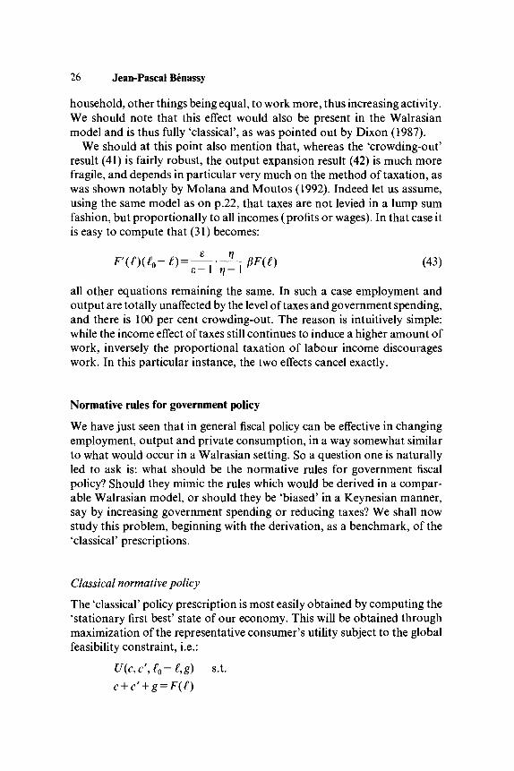
We should at this point also mention that, whereas the 'crowding-out'result (41) is fairly robust, the output expansion result (42) is much morefragile, and depends in particular very much on the method of taxation, aswas shown notably by Molana and Moutos (1992). Indeed let us assume,using the same model as on p.22, that taxes are not levied in a lump sumfashion, but proportionally to all incomes (profits or wages). In that case itis easy to compute that (31) becomes:
(43)
all other equations remaining the same. In such a case employment andoutput are totally unaffected by the level of taxes and government spending,and there is 100 per cent crowding-out. The reason is intuitively simple:while the income effect of taxes still continues to induce a higher amount ofwork, inversely the proportional taxation of labour income discourageswork. In this particular instance, the two effects cancel exactly.
Normative rules for government policy
We have just seen that in general fiscal policy can be effective in changingemployment, output and private consumption, in a way somewhat similarto what would occur in a Walrasian setting. So a question one is naturallyled to ask is: what should be the normative rules for government fiscalpolicy? Should they mimic the rules which would be derived in a compar-able Walrasian model, or should they be 'biased' in a Keynesian manner,say by increasing government spending or reducing taxes? We shall nowstudy this problem, beginning with the derivation, as a benchmark, of the'classical' prescriptions.
Classical normative policy
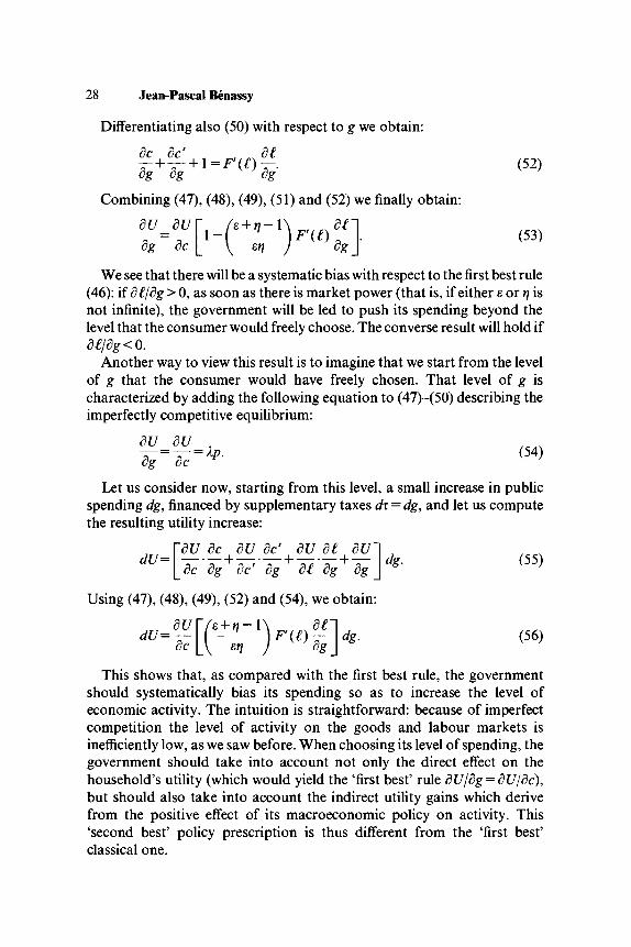
The 'classical' policy prescription is most easily obtained by computing the'stationary first best' state of our economy. This will be obtained throughmaximization of the representative consumer's utility subject to the globalfeasibility constraint, i.e.:
U(c,c'J0-£,g) s.t.

Classical and Keynesian features 27
which yields the conditions:
8U dU dU 1 dUdc dc' dg F(£)d(£0-£)'
(44)
It is easy to verify that this first best solution can be obtained as astationary Walrasian equilibrium, corresponding to (22)-(28) taking both1/6 and l/rj equal to zero, provided the government adopts the followingrules:
g = T (45)
eg dc
(45) simply tells us that the government's budget should be balanced. (46)tells us that the government should push public spending to the point whereits marginal utility is equal to that of private consumption. In other wordsthe government should act as a 'veil' and pick exactly the level of g thehousehold would have chosen if it was not taxed and could purchasedirectly government goods.
Normative policy under imperfect competition
We shall now derive the optimal rule for the government under imperfectcompetition. In order to simplify analysis, we shall study only the balancedbudget case g = T.3 In that case, prices are constant in time and equations(22)-(28) simplify to:
"(£) (47)
(49)
g=y = F(£). (50)
All equilibrium values depend on the level of g chosen by the govern-ment. To find its optimal value, let us differentiate U(c,c',£Q—£,g) withrespect to g:
dU dc dU dc' dU dl dU_
28 Jean-Pascal Benassy
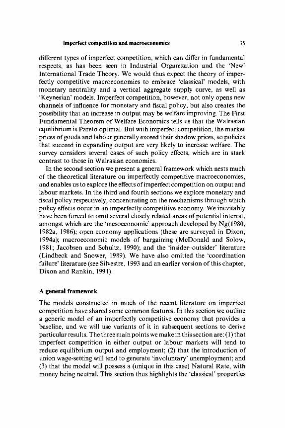
Differentiating also (50) with respect to g we obtain:
p ? f S < ( 5 2 )g
Combining (47), (48), (49), (51) and (52) we finally obtain:dU dUV /e + w - r (53)
We see that there will be a systematic bias with respect to the first best rule(46): if d£/dg> 0, as soon as there is market power (that is, if either s or rj isnot infinite), the government will be led to push its spending beyond thelevel that the consumer would freely choose. The converse result will hold ifd£/dg<0.
Another way to view this result is to imagine that we start from the levelof g that the consumer would have freely chosen. That level of g ischaracterized by adding the following equation to (47)-(50) describing theimperfectly competitive equilibrium:
Let us consider now, starting from this level, a small increase in publicspending dg, financed by supplementary taxes dx = dg, and let us computethe resulting utility increase:
VdU dc dU dc1 dU dl dUldU==\ lT-lT + ^ - X - f T 7 ' ^ r + T-[_dc dg dc dg dl dg dg J
Using (47), (48), (49), (52) and (54), we obtain:
This shows that, as compared with the first best rule, the governmentshould systematically bias its spending so as to increase the level ofeconomic activity. The intuition is straightforward: because of imperfectcompetition the level of activity on the goods and labour markets isinefficiently low, as we saw before. When choosing its level of spending, thegovernment should take into account not only the direct effect on thehousehold's utility (which would yield the 'first best' rule dU/dg = dU/dc),but should also take into account the indirect utility gains which derivefrom the positive effect of its macroeconomic policy on activity. This'second best' policy prescription is thus different from the 'first best'classical one.

Classical and Keynesian features 29
Should one, however, believe that the normative policy is biased in a'Keynesian' manner? This is not the case, at least for two reasons. First,even when d-E/dg is positive, what leads to the activity increase is notgovernment spending per se via a 'Keynesian' demand multiplier, butrather the taxes levied to finance them via a 'classical' labour supply effect.Normative analysis would then somehow call for higher taxes, hardly aKeynesian prescription. Secondly, the magnitude and even the sign of df/dgdepends enormously on the method of taxation, making the direction of thebias extremely difficult to assess. Using again the example on pp.22 and 26,under proportional taxation the government should use exactly the 'classi-cal' prescription. So whatever bias exists in the normative prescriptions, it isdefinitely not of a Keynesian type.
Conclusions
We constructed in this chapter a simple prototype model of imperfectcompetition with rational expectations and objective demand curves,studied its various properties, and compared them with those of the basic'classical' and 'Keynesian' models.
We may first note that this model of imperfect competition clearlygeneralizes the corresponding Walrasian one, which can be obtained as alimit case by making the parameters rj and a go to infinity.
As for the 'positive' properties of the model, we saw that they standsomehow halfway between the Keynesian and classical ones: the inef-ficiency properties very much resemble those of a Keynesian fix-price-fix-wage model. On the other hand, the response to government policy, fiscal ormonetary, is very much of a 'classical' nature.
The normative implications of such models for government action arealso very important, and we saw that they were neither Keynesian norclassical. Moreover simple variations on the above model show that theywill depend crucially on the nature of rigidities in the price system. It is thusquite urgent to develop models with more sophisticated rigidities than thosearising from simple market power and to explore their positive andnormative properties. This should be the object of further research.
Appendix
We shall in this appendix derive, under a more general form, the objectivedemand curves used in the text (cf. notably (16) and (17)), and show how allthe results extend without modification to general aggregator functions Aand V.

30 Jean-Pascal Benassy
The objective demand curves
When computing the objective demand curve for the product he sells, eachprice-maker has to forecast the demand forthcoming to him for any valueof (1) the price or wage he determines and (2) prices and wages set by otheragents. Following the methodology developed in Benassy (1988, 1990), wesee that the natural definition of objective demand at a price-wage vector(P, W) is simply the demand forthcoming at a fix-price equilibriumcorresponding to (P, W), which we shall now compute.
We may note before actually starting computations that, according to atraditional result in imperfect competition, each agent will set the price ofthe good he controls at a level high enough for him to be willing to serve alldemand forthcoming, and actually even more. We are thus, in 'fix-price'terminology, in a situation of generalized excess supply where each agent isconstrained in his supply (but unconstrained in his demand) and thus takesthe level of his sales as a constraint.
Consider first firmy. For given prices and wages its optimization programis:
s.t.
where y}is determined by the demand of other agents and thus exogenous tofirm/ The solution in ltj to this program is:
£ij=(j>i{W)F-\yj) (Al)
where <t>i(W), a function associated to A by duality, is homogeneous ofdegree zero in its arguments. As an example, if A is the CES function (3),then
J(lf (A2)
where w is the aggregate wage index given by (4) in the text.Consider now old household /. It owns a quantity of money mt and seeks
to maximize its second-period consumption index c\ (8) under the budgetconstraint:
7=1

Classical and Keynesian features 31
The result of this maximization is:
c',= <t>j(P)^ (A3)
where </>//>)> associated by duality to F, is homogeneous of degree zero inall prices, and/? is the aggregate price index associated to F, given by:
A (A4)
As an example again, if Fis the CES function (10), then:
• ( A 5 )
Consider now the government and assume it has chosen a level gt for thelevel of public consumption index attributed to household /. The govern-ment will choose the specific gtJs to minimize the cost of doing so, and willthus solve the program:
7=1
which yields the solution in gtj:
(A6)
where <t>j(P) is the same as in (A3). The cost to the government is pgt.Let us finally consider young household /. Merging its two budget
constraints (12) and (13) into a single one, we find that it will determine itscurrent consumptions ctj through the following maximization program:
max Uic^c-Jo-^gt) s.t.
where the right-hand side (and notably the quantity tt of labour sold) isexogenous to household /. Given the assumptions on U (separability,homotheticity), the solution will be such that the value of current consump-tions is given by:
n
£i + n-pti) (A7)

32 Jean-Pascal Benassy
where y(p'/p) is the propensity to consume. Maximizing ct under budgetconstraint (A7) yields the current consumptions ctj:
cv=<l>j(P)y(p'lp)M+n-ini)- (A8)We have now determined all components of the demand for goods.
Output yj will be equal to the sum of demands for goody, i.e.:
which, using (A3), (A6) and (A7) yields:
1=1
G=£gl M=£mi e=£r, (A10)1 = 1 / = 1 1 = 1
We shall use the global incomes identity:
X(w^.+7r,0=Z/y> (All)i=i j=\
Combining (A4), (A 10) and (Al 1) we obtain the final expression for theobjective demand addressed to firm j :
M
If the number n of producers is large, /?, p' and thus y are taken asexogenous to firm 7 and the elasticity of Yf with respect to pf is that of thefunction (j>r
We can now compute the objective demand for type / labour by addingthe Ifij = 1,...,« given by (A1) and replacing y^ by the objective demand Yjjust derived, which yields:
j (A13)7=1
where the Yj are given by (A 12). Again with large n, the elasticity of Lt withrespect to wt is equal to that of 0f( W).
Now formulas (16) and (17) in the text are simply obtained by replacing0,( W) and (j)j(P) by the specific forms (A2) and (A5), and using the fact thatthe values of AW,-, gt and T, are the same for all n households.

Classical and Keynesian features 33
General aggregator functions
We shall now show that all results derived in the text with the specific CESaggregator functions (3) and (10) are valid as well with general forms for Aand V, and notably that the crucial (22) and (25) hold unchanged.
Indeed the first order conditions for programs (Aj) and (A() are in thegeneral case:
H'-*yi <A14)PlTT / 1\
(A15)
where r\j and e, are the absolute values of the elasticities of the functions Y,and Lt. Looking at formulas (A 12) and (A 13), we see that for large n theseelasticities are actually those of the functions <f>j and (/>,-, so that:
rir-d log <t>j(P)/d log Pj=Yij{P) (A16)
£,= - a log <t>t(W)ld log w^e^W) (A17)
Because of the homogeneity and symmetry properties of the originalfunctions A and V these elasticities are the same at all symmetric points, andwe denote them as rj and s:
flj(j>9...,p) = ri V/7,V7 (A18)
8/(w,...,w) = e Vw,W. (A 19)
Combining (A 14), (A 15), (A 18) and (A 19) at a symmetric equilibrium,we obtain (22) and (25).
Notes
I wish to thank Huw Dixon and Neil Rankin for their comments on a first version ofthis chapter. The usual disclaimer applies fully here.1. Of course all the concepts that follow would be valid with a different number of
households and firms, but using the same number n will simplify notation at alater stage.
2. These were initially introduced in the macrosetting by Weitzman (1985).3. The case of an unbalanced budget g¥"c is studied in Benassy (1991b).

2 Imperfect competition andmacroeconomics: a survey
Huw David Dixon and Neil Rankin
Introduction
The importance of imperfect competition has long been recognized in manyareas of economics, perhaps most obviously in industrial economics and inthe labour economics of trade unions. Despite the clear divergence ofoutput and labour markets from the competitive paradigm in mostcountries, macroeconomics where it has used microfoundations has tendedto stick to the Walrasian market-clearing approach. However, over the lastdecade a shift has begun away from a concentration on the Walrasian price-taker towards a world where firms, unions and governments may bestrategic agents. This chapter takes stock of this burgeoning literature,focusing on the macroeconomic policy and welfare implications of imper-fect competition, and contrasting them with those of Walrasian models.
We seek to answer three fundamental questions. (1) What is the nature ofmacroeconomic equilibrium with imperfect competition in output andlabour markets? With monopoly power in the output market causing priceto exceed marginal cost, and union power leading to the real wageexceeding the disutility of labour, we would expect imperfectly competitivemacroeconomics to have lower levels of output and employment thanWalrasian economies, a Pareto inefficient allocation of resources, and thepossibility of involuntary unemployment. Few would disagree that devi-ations from perfect competition will probably have undesirable conse-quences. (2) To what extent can macroeconomic policy be used to raiseoutput and employment in an imperfectly competitive macroeconomy? (3)If policy can raise output and employment, what will be the effect on thewelfare of agents?
Whilst there may be fairly general agreement over the answer to (1), webelieve that there are no truly general answers to (2) and (3). In Walrasianmodels there is only one basic equilibrium concept employed: prices adjustto equate demand and supply in each market. There are, however, many
34
Imperfect competition and macroeconomics 35
different types of imperfect competition, which can differ in fundamentalrespects, as has been seen in Industrial Organization and the 'New'International Trade Theory. We would thus expect the theory of imper-fectly competitive macroeconomics to embrace 'classical' models, withmonetary neutrality and a vertical aggregate supply curve, as well as'Keynesian' models. Imperfect competition, however, not only opens newchannels of influence for monetary and fiscal policy, but also creates thepossibility that an increase in output may be welfare improving. The FirstFundamental Theorem of Welfare Economics tells us that the Walrasianequilibrium is Pareto optimal. But with imperfect competition, the marketprices of goods and labour generally exceed their shadow prices, so policiesthat succeed in expanding output are very likely to increase welfare. Thesurvey considers several cases of such policy effects, which are in starkcontrast to those in Walrasian economies.
In the second section we present a general framework which nests muchof the theoretical literature on imperfectly competitive macroeconomics,and enables us to explore the effects of imperfect competition on output andlabour markets. In the third and fourth sections we explore monetary andfiscal policy respectively, concentrating on the mechanisms through whichpolicy effects occur in an imperfectly competitive economy. We inevitablyhave been forced to omit several closely related areas of potential interest,amongst which are the 'mesoeconomic' approach developed by Ng(1980,1982a, 1986); open economy applications (these are surveyed in Dixon,1994a); macroeconomic models of bargaining (McDonald and Solow,1981; Jacobsen and Schultz, 1990); and the 'insider-outsider' literature(Lindbeck and Snower, 1989). We have also omitted the 'coordinationfailure' literature (see Silvestre, 1993 and an earlier version of this chapter,Dixon and Rankin, 1991).
A general framework
The models constructed in much of the recent literature on imperfectcompetition have shared some common features. In this section we outlinea generic model of an imperfectly competitive economy that provides abaseline, and we will use variants of it in subsequent sections to deriveparticular results. The three main points we make in this section are: (1) thatimperfect competition in either output or labour markets will tend toreduce equilibrium output and employment; (2) that the introduction ofunion wage-setting will tend to generate 'involuntary' unemployment; and(3) that the model will possess a (unique in this case) Natural Rate, withmoney being neutral. This section thus highlights the 'classical' properties

36 Huw David Dixon and Neil Rankin
of imperfect competition, as a prelude to subsequent sections which willextend the framework to models with less classical effects for monetary andfiscal policy.
There are n produced outputs Xi,i=l,...,n. Households' utility functiontakes the form
[u(Xl,...,Xn)]c[M/P\l~c-0Ne 0 < c < l , e > l (1)where u is a degree-one homogeneous subutility function, P is the cost-of-living index for u, M is nominal money holdings, and 9Ne is the disutility ofsupplying N units of labour, N<H. Since preferences are homothetic overconsumption and real balances we can aggregate and deal with one'representative' household. Most studies further simplify (1). First, aspecific functional form is assumed for u(-) - notably Cobb-Douglas orCES. Second, the labour supply decision may be made a [0,1] decision - towork or not to work for each individual household. We can represent thisfor our aggregated household by setting e= 1, so that 6 is the disutility ofwork. Most models of imperfect competition incorporate money using thestandard temporary equilibrium framework (see Grandmont, 1983, for anexposition) by including end-of-period balances in the household's utilityfunction. Whether it should be deflated by the current price level as in (1)depends on the elasticity of price expectations, as we discuss on p.47 below.As regards firms, we assume there are F firms in sector /, each with aloglinear technology
XirB~xN« f a<\. (2)
The special case of constant returns where a= 1 is widely used.1We have now to add the macroeconomic framework. Turning first to
aggregate income-expenditure identities, income in each sector must equalexpenditure Yt on that sector, and national income must equal totalexpenditure Y. We will introduce fiscal policy in the fourth section. In thissection, the government merely chooses the total money supply Mo. Inaggregate, the household's total budget consists of the flow component Yand the stock of money Mo. Given (1), households will choose to spend aproportion c of this on producer output, and to save a proportion 1 — c toaccumulate money balances M? Hence the income-expenditure identitiescoupled with (1) imply that in aggregate:
Y=c[M0+Y] or Y=-^-cM0. (3)
Given total expenditure, households allocate expenditure across the pro-duced goods. Since preferences are homothetic, the budget share of output

Imperfect competition and macroeconomics 37
z, a,, depends only on relative prices. Hence total expenditure on sector /, Yi9is given by
PiXi=Yi = *i(Pl9...,PJY (4)where oct is homogeneous of degree zero in Pu...,Pn. We will assumesymmetric preferences, so that if all prices of outputs are the same then
How are wages and prices determined? As a benchmark let us considerthe Walrasian economy with price-taking households and firms. Further-more, let us assume perfect mobility of labour across sectors, so that there isa single economy-wide market and wage W. The labour supply from (1) isthen
NS(W/P)= [6e]m]~e][W/P]l/[e~l\ (5)The additive separability combined with degree-one homogeneity of (1)rules out any wealth effect on labour supply, so that only real wages matter.Assume a single, representative, price-taking firm per sector.3 Then sectorfs labour demand takes the form
N\WjPi)= [a/BY^-^W/P;]-^1-^. (6)In a symmetric equilibrium where Pt= P, (5)-(6) determine equilibrium realwages, employment and output in the representative sector. Equilibriumsector output X* is given by B~l[N*]a. Under symmetry a,= l/n in (4) sothat the nominal price level is
p ( 7 )1-cnX* {)
Nominal wages and prices adjust to equate aggregate demand withequilibrium output. This is an entirely 'classical' model with full employ-ment and neutral money.
What difference does the introduction of imperfect competition make?Let us assume that each output is monopolized by a sole producer (F= 1)and that there are many sectors. The large '«' means that the monopolisttreats the general price index P as exogenous when it makes its decisions.Before we proceed, it should be noted that the elasticity of demandfi/(jPi,..., Pn) = — [31niydlnPJPconst from (4) is homogeneous of degree zeroin prices, due to homotheticity. In a symmetric equilibrium ei(Pl,...,Pn)will thus take the same value irrespective of the price level: s* = ( 1 , . . . , 1). Wewill assume gross substitutability in general, so that e* > 1. If the individualfirm maximizes its profits treating the general price level as given, then itslabour demand is easily obtained as

38 Huw David Dixon and Neil Rankin
W/P
Nm Nc N
Figure 2.1 Equilibrium with and without monopolistic firms
Ndm(w/pi)= [i - (8)
Since e* > 1 and a < 1, labour demand is smaller for any given real wage, aswe would expect. Equilibrium under symmetry is depicted in figure 2.1. Fora given supply curve, in a symmetric equilibrium the effect of monopolisticcompetition is simply to reduce sectoral employment (and hence output)from Nc to Nm. Note that money will still be neutral, since (5) and (8) areboth homogeneous of degree zero in (W,P). The degree of monopoly \i isI/a*. So the less elastic is demand when prices are all equal, the higher themarking up of price over marginal cost and the lower equilibrium output.Imperfect competition in the output market has thus reduced total outputand employment, although (since the labour market is competitive) house-holds are on their labour supply curve Ns.
How will the introduction of unions alter matters? To take the simplestcase, consider an economy-wide monopoly union that has the unilateralpower to set the nominal wage. The union predicts, given the wage it has set,what prices will be set by firms and the resultant level of employment.4 Atthe aggregate level, the trade-off between real wages and employment facedby unions in symmetric equilibrium is given by (8) multiplied by the numberof sectors n. Several assumptions may be made about union preferences (seeOswald, 1985). Here we will simply assume that the union's objectivefunction is to maximize the total surplus, or wage revenue less disutility,earned by employed workers.5 If we let e=l, then there is a constantmarginal disutility of labour 6. Each employed worker earns W/P-6 assurplus. The union's problem is thus
max[ W/P- 6]Ndm(JV/P). (9)
Since the elasticity of labour demand with respect to W/P is constant in (8),

Imperfect competition and macroeconomics 39
W/P
(w/py
Nu N
Figure 2.2 Equilibrium with an economy-wide union
the solution to (9) has the property that the union chooses the real wage as aconstant mark-up over 6
W/P = 0/a. (10)This is depicted in figure 2.2, where we show the union's maximum utilityindifference curve U*. The less elastic is the demand for labour (the lower a),the higher is the wage set by the union. Since the monopolistic andcompetitive firms have the same real wage elasticity of labour demand, thereal wage chosen by the union is the same, though employment is lower withmonopolistic firms. Again, since (10) is homogeneous of degree zero in(W, P), money is neutral. This model illustrates the point that the introduc-tion of wage-setting unions leads to involuntary unemployment. Since theunion marks up the wage over the disutility of labour (from (10)), theunemployed households are worse off than the employed, and furthermorethe employed would be willing to work more for less.
Turning to the case of sectoral unions, wages in each sector may nowdiffer. The union is assumed to control entry into employment in thatindustry so that employed 'insiders' are isolated from the potential compe-tition of'outsiders' (see Lindbeck and Snower, 1989, for a discussion). In alarge economy with many sectors, each individual union will take thegeneral price level of goods consumed by its members as given (in contrastto the centralized union) and in a non-cooperative Nash framework it willalso treat other sectoral unions' wages as given. However, each union willtake into account the effects of its wages on its own sector's price Pt andhence on output and demand for labour in its sector. The sectoral labourdemand curve is thus essentially a relation between nominal wages Wt andemployment, because the firm bases its employment on the own-productwage WJPi9 in contrast to the union's objective function which depends onthe real consumption wage WJP.6

40 Him David Dixon and Neil Rankin
Consider the elasticity of the sectoral unions' demand for labour withrespect to Wt. The labour-demand equation stems from the price-costequation which equates the own-product wage to the marginal revenueproduct of labour
^=—aB-lNtrV-°\ (lla)
If we take logs and differentiate Nt with respect to Wh taking into accountthat P/depends upon Xxwhich depends upon Ni9 we obtain the money-wageelasticity of labour demand as
iy]/c V '
where rj is the elasticity of [e— l]/e with respect to Pi9 which captures theeffect of a rise in Wt (and hence Pt) on the mark-up of price over marginalcost, e/[e—\]. This can take either sign, although it is perhaps morereasonable to assume that de/dPt>0 (demand becomes more elastic as youraise price), so that rj > 0 (the mark-up falls as Wxrises). If the sectoral unionmaximizes its surplus with respect to Wh subject to the labour demandimplicitly defined by (11), the equilibrium real wage given symmetry acrosssectors is
This is a higher real wage than with the centralized union (cf. (10)) so long asrj < 1. If utility is CES then s(Pl9...,Pn) is equal to the constant elasticity ofsubstitution, so rj = 0 and the comparison of (12) with (10) is unambiguous.
The sectoral union thus tends to set a higher nominal wage, with aconsequent lower level of employment, despite the fact that the money-wage elasticity of its labour demand is likely to be higher than for acentralized union.7 The reason is that it sees no effect of its own behaviouron the general price level P at which its members consume. A centralizedunion takes the general rise in P which it causes into account, and sorestrains its wage pressure. This can also be seen as an example ofexternalities: the price rise caused by a sectoral union is mostly borne bymembers of other unions. For a detailed discussion of the effect of differentunion structures on wage determination, see Calmfors and Driffill (1988).
An alternative to sectoral unions - which are organized by industry - arecraft unions, which are organized by labour skills. Blanchard and Kiyotaki(1987) use these. Each union sells a different type of labour, some of which isrequired by every firm. The number of labour types is assumed large, soeach Wh has a negligible effect on the general index of wages W and no

Imperfect competition and macroeconomics 41
W/PN*
Nd
Nm Nm N
Figure 2.3 Equilibrium with craft unions and monopolistic firms
union sees itself as affecting any firm's output. Firm fs demand for type hlabour, which is obtained by minimizing the cost of producing a givenoutput Xh is
Nih = kn[WJWr°Xt/a *„ = const (13)
where a(> 1) is the constant elasticity of technical substitution betweenlabour types. Blanchard and Kiyotaki further assume increasing marginaldisutility of work, i.e. e> 1 in (1), so that the union's surplus is8
[Wh/P]Nh-6Neh. (14)
Maximizing (14) subject to (13) (aggregated over all /) taking W andXi9..., Xn as given, union h chooses the level of labour sales
n=[\-l/a]l/[e-l]Ns(Wh/P).Nst (15)
Since a>\, labour sales are smaller for any given real wage than in thecompetitive case (5), as we would expect. Combining (15) with (8) deter-mines equilibrium under symmetry amongst firms and unions, as in figure2.3. Whether the employment level is higher or lower than with sectoralunions depends on technological substitutability between labour types.With rj = O and e = 1, employment is lower ifcr<l/[l — a[\ — 1 /e]]. Money isclearly still neutral.
In this section we have presented a simple general framework thatcaptures some common features of much of the recent work on imperfectcompetition and macroeconomics. We will now proceed to see howextensions of this general framework yield less orthodox results.
Monetary policy
Imperfect competition by itself does not create monetary non-neutrality, aswe have seen.9 It is the combination of imperfect competition with some

42 Him David Dixon and Neil Rankin
other distortion10 which generates the potential for real effects. The natureof this other distortion provides us with a natural method for classifyingmodels of monetary policy effectiveness. First, the largest part of theliterature combines imperfect competition with small lump sum costs ofadjusting prices ('menu' costs), which are intended to represent theadministrative costs of printing new price lists, etc. Examples of thisapproach are Mankiw (1985), Akerlof and Yellen (1985a), Blanchard andKiyotaki (1987), Benassy (1987), Caplin and Spulber (1987), Ball andRomer (1989a, 1990, 1991). A second group of studies may be interpretedas taking the same general framework of imperfect competition in amonetary temporary equilibrium, but as relaxing an implicit assumptionoften unconsciously made there: namely, that of unit-elastic expectations offuture with respect to current prices. These include the seminal study ofHart (1982) and applications and extensions by Dehez (1985), d'Aspremontet al (1989a, 1990), Silvestre (1990) and Rankin (1992, 1993). Thirdly,studies by Dixon (1990b, 1992), Fender and Yip (1993), and Moutos (1991)look at the imperfect competition combined with a small nominal rigidity insome sector of the economy. Common to all three approaches is that thesame distortions in the presence of perfect competition would not causemonetary policy to affect output significantly. It is the interaction betweenminor, and perhaps intrinsically uninteresting, distortions and imperfectcompetition which generates major departures from neutrality. This can beviewed as an instance of the theory of the second best at work: monetarypolicy is not capable of causing Pareto improvements given either imperfectcompetition or the other distortion on its own, but given both together, it is.
Menu costsWe take Blanchard and Kiyotaki's (1987) model for our illustration,though the central ideas appear first in Mankiw (1985) and Akerlof andYellen (1985a). Very similar points were simultaneously made by Benassy(1987), and Parkin's (1986) study also has strong parallels. That thisapproach has also been influential outside the realm of pure theory is shownby Layard and Nickell's adoption of the Blanchard-Kiyotaki frameworkfor their widely known empirical studies of UK unemployment (Layardand Nickell, 1985,1986; Layard, Nickell and Jackman, 1991). The model inthe absence of menu costs has already been described. Suppose now that theprice- and wage-setting agents face administrative costs of changing pricesand wages (e.g. for a restaurant, the cost of reprinting its menus). Such costsare lump sum in nature: they do not depend on the size of the price or wagechange. If they are large enough to outweigh the forgone profits or utility ofnot adjusting a price or a wage when an increase in the money supply
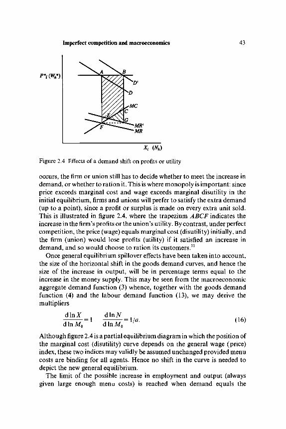
Imperfect competition and macroeconomics 43
P*i(Wh*)
Figure 2.4 Effects of a demand shift on profits or utility
occurs, the firm or union still has to decide whether to meet the increase indemand, or whether to ration it. This is where monopoly is important: sinceprice exceeds marginal cost and wage exceeds marginal disutility in theinitial equilibrium, firms and unions will prefer to satisfy the extra demand(up to a point), since a profit or surplus is made on every extra unit sold.This is illustrated in figure 2.4, where the trapezium ABCF indicates theincrease in the firm's profits or the union's utility. By contrast, under perfectcompetition, the price (wage) equals marginal cost (disutility) initially, andthe firm (union) would lose profits (utility) if it satisfied an increase indemand, and so would choose to ration its customers.11
Once general equilibrium spillover effects have been taken into account,the size of the horizontal shift in the goods demand curves, and hence thesize of the increase in output, will be in percentage terms equal to theincrease in the money supply. This may be seen from the macroeconomicaggregate demand function (3) whence, together with the goods demandfunction (4) and the labour demand function (13), we may derive themultipliers
dlnM1 d l n N 1/;=1 d^rlla- (16)
Although figure 2.4 is a partial equilibrium diagram in which the position ofthe marginal cost (disutility) curve depends on the general wage (price)index, these two indices may validly be assumed unchanged provided menucosts are binding for all agents. Hence no shift in the curve is needed todepict the new general equilibrium.
The limit of the possible increase in employment and output (alwaysgiven large enough menu costs) is reached when demand equals the

44 Huw David Dixon and Neil Rankin
competitive supply in either market. Beyond this, even monopolistic agentswill choose to ration any further increase. Whether the limit is first hit in thegoods or labour market depends whether the real wage is above or below itsWalrasian level (respectively). In figure 2.3, for example, the maximumemployment level as Mo is increased occurs at Nm\ where the supplyconstraint in the labour market becomes binding. This brings out theformal similarity between the menu cost models and the 'disequilibrium'models of the 1970s (Barro and Grossman, 1971; Benassy, 1975; Malin-vaud, 1977 - see Benassy, 1990 for a more recent survey). Within the class ofequilibria for which menu costs bind, the economy behaves exactly as if itwere in a quantity-constrained equilibrium.12 In particular, within theneighbourhood of the initial frictionless equilibrium, it behaves as if in aregime of generalized excess supply, or 'Keynesian unemployment'. Bigincreases in the money supply will shift it into a regime of 'repressedinflation' (as happens in figure 2.3) or 'classical unemployment', dependingon whether labour or goods supply constraints are reached first. Thissimilarity between excess supply and monopoly was first exploited byBenassy (1976, 1978) and Negishi (1979) as a means to 'endogenize' pricesin disequilibrium models. Their models, however, use the concept of'subjective' demands, introduced by Negishi (1961), rather than the 'objec-tive' demands used here.
Note that the increase in output also constitutes a Pareto improvement.This is for three reasons: first, the shift in demand for labour brings a utilitygain to the household equal to the area ABCF in figure 2.4; second,households receive an increase in profits from firms; and third, real moneybalances increase, which increases households' utility directly. An interest-ing interpretation of the Pareto suboptimality of the initial monopolisticequilibrium is to view it as resulting from a lack of cooperation amongstprice-setting agents. Benassy (1987) and Blanchard and Kiyotaki (1987)both point out that an agreement by all firms and households simulta-neously to lower their prices and wages by x per cent would produce exactlythe same real reallocation as a money supply increase of x per cent in thepresence of binding menu costs. In either case real balances, and thus realdemand and output, rise by x per cent, with no relative price changes.Monetary policy can thus be seen as a substitute for a cooperativeagreement to lower prices. The failure to lower prices when actingindependently is explained by Blanchard and Kiyotaki as due to an'aggregate demand externality':13 a lowering of one agent's price benefits allothers to the extent that it slightly reduces the general price index and soraises real money balances and aggregate demand.14 However, the privategain to the price-cutter is outweighed by the private loss due to the too-lowrelative price which would result. The monopolistically competitive equili-

Imperfect competition and macroeconomics 45
brium is therefore a form of economy-wide 'Prisoner's Dilemma'. In theabsence of menu costs, when to expand the money supply would have nobeneficial effect, a welfare-enhancing measure would be to impose an all-round wage and price cut by a prices and incomes policy.
Before the menu cost model can be taken seriously, it must tackle theobvious objection that in practice administrative costs of price and wageadjustment are very small. Because such costs are lump sum, once they aredominated by the forgone profits or utility of not re-optimizing in the faceof a money supply increase, they will have no effect at all: an agent who hasdecided to adjust her price will adjust it to the same level as in the absence ofmenu costs, since the cost depends on the fact of the adjustment and not onits size. A large part of the research into menu costs has been concerned withovercoming this objection. The key observation is provided by Akerlof andYellen (1985a) and Mankiw (1985), who point out that the opportunity costof non-adjustment is second order in the size of the money supply shock.That is, if we take a Taylor approximation to firm /'s forgone profits of notincreasing Pi9 or to union h's forgone utility of not increasing Wh, it willcontain no term in AM0, only in (AM0)2 and higher powers of AMQ. Weexplain why below. By comparison, the increase in output is first order, i.e.proportional to AM0, as is clear from (16). Thus, as AMQ tends to zero, theratio of the size of menu cost necessary for non-adjustment to the change inoutput which it sustains also tends to zero. For non-infinitesimal but smallchanges in the money supply, it follows that only a very small menu cost willbe required in order to sustain non-adjustment. For instance, Blanchardand Kiyotaki's calculations show that with a 5 per cent money supplyincrease and 0 = 0-= 5, e=\.6 and # = 0.8, the minimum menu cost forhouseholds to prefer non-adjustment is equal to only 0.112 per cent ofGDP, and for firms to only 0.018 per cent of GDP.
To see why the opportunity cost is second order, consider again figure2.4. (We have deliberately magnified the diagram in the neighbourhood ofequilibrium, which permits us to approximate curves as straight lines.) Ifthe price were to be adjusted following the shift in demand, the new outputwould be determined by the intersection E. Since output under noadjustment is greater than this, the forgone profits (utility) of not adjustingare measured by the cumulated surplus of MC over MR', given by triangleCGE. As the size of AM0, and thus of the demand shift AB, is squeezedtowards zero, the area of this triangle clearly falls with the square of AB,and thus with the square of AM0 (note that distance BG always equals AFsince demand elasticity is a constant). Intuitively, the reason why the cost isonly second order is that 'objective functions are flat on top': in theneighbourhood of a maximum the slope is close to zero, so that the lossfrom being only slightly away from the optimum is also very close to zero.

46 Hun David Dixon and Neil Rankin
Several extensions of this basic analysis are made by Ball and Romer. Intheir (1989a) study, they show that if the money supply is stochastic then thewelfare cost of price rigidity, as measured by the fall in expected utility,becomes second rather than first order, i.e. proportional to the variance ofthe money supply. Despite this, parameter values exist which will drive theratio of second order menu costs to second order welfare losses to zero.15 Intheir 1991 study, Ball and Romer show that for a given money supplyincrease, there exists an intermediate range of values for the menu cost suchthat two equilibria coexist: one with no and one with full price adjustment.For menu costs in this range it can thus be argued that if the outcome is noadjustment, price rigidity is due to a coordination failure: if each agentexpected the others to adjust, she would want to adjust too. In yet a thirdstudy, Ball and Romer (1990) address the problem for the basic menu costmodel that, although theoretically acceptable parameter values exist whichkeep rigidity-sustaining menu costs small, these values are still unrealisticempirically. The lowest value of competitive labour supply elasticity(l/[e - 1]) used in Blanchard and Kiyotaki's numerical illustrations is If (asin the cited example), which is much higher than most econometricestimates. Ball and Romer suggest a solution by showing that rigidities innominal prices are made more likely if there are also rigidities in real - orrelative - prices. Their general argument is as follows. Suppose agent / hasthe indirect utility function
Ut=W(MJP9PJP). (17)
Agents in the model are 'farmers'.16 fs optimum relative price is clearlydetermined from the first order condition W2(M0/P,P?/P) = 0 (the subs-cript denoting a partial derivative), whence
d(P*/P)/d(MQ/P)= - Wn\W12 (EETT, say). (18)(+) (-)
If a change in aggregate demand causes only a small change in fs desiredrelative price, real rigidity is said to be 'high', so n is an inverse measure of it.The second order approximation to /'s private utility cost of not adjustingPt after a change AM0, given that others do not adjust, is
PCK[-{Wn)2l2W12\[AM0]2=\nWu[AM,]2. (19)
Thus the smaller is n, i.e. the greater the real rigidity, the smaller is the menucost needed to ensure that / does not adjust his price. Ball and Romer fleshout this simple framework with two explicit models of real rigidities: a'customer market' model in which firms face kinked demand curves due toignorance by their customers of prices elsewhere; and a model with an'efficiency wage' in the labour market.17 Hence by combining three 'distor-

Imperfect competition and macroeconomics 47
tions' - imperfect competition, menu costs and real rigidities - an empiri-cally plausible model of non-neutrality can be obtained.18
Are the results modified in a dynamic setting? Caplin and Spulber (1987)and Caplin and Leahy (1991) examine this question. Rules for optimalprice- and wage-setting over time when subject to menu costs take an 'Ss'form: when the deviation of Pt from its no-menu cost optimum, P* whichfollows a stochastic process determined by the process for the moneysupply, hits a ceiling S or a floor s9 an adjustment is made to Pi9 bringingPf— Pt back to some 'return point'. Caplin and Spulber show that when themoney supply process involves only non-negative shocks to the moneystock, money - rather surprisingly - turns out to be neutral in the aggregate.However when the process is symmetric, allowing negative as well aspositive shocks, shocks do affect aggregate output, as shown in Caplin andLeahy.19 Although these models are dynamic, the firm's optimizationproblem is treated as static. Dixit (1991), in a partial equilibrium analysis,shows that with dynamic optimization menu costs as small as fourth ordercan sustain price rigidities. The considerable difficulties of aggregatingacross agents with different initial situations have, however, so far discour-aged the rapid development of this branch of the literature.
Non-unit-elastic price expectations
Hart (1982) was the first to show that imperfect competition could generatepolicy effectiveness. The 'policy' he considers, however, is not strictlymonetary policy at all: it is an increase in the stock of a 'non-produced'good. Although Hart is reluctant to interpret this as 'money', we can validlydo so if we view Hart's framework as one of temporary monetaryequilibrium in the manner of Patinkin (1965) and Grandmont (1983). Inthis case the key assumption necessary for monetary policy effectiveness isthat - implicitly or explicitly - agents' expectations of future prices are 'non-unit-elastic' in current prices. We present here a simple version of Hart'smodel under this monetary reinterpretation. We also examine anotherquestion debated in the literature for which Hart's model has been theframework: whether imperfect competition in the goods market can causeunemployment even at a zero wage.
Relative to the second section we slightly modify the household'sproblem, to
ma.xu(X,M/Pe) subj to MQ+Y=PX+M. (20)
Pe is the subjective expectation of next period's price level, so M/Pe isexpected future consumption (taking the simplest possible case, in whichthe household has no future income).20 Our earlier utility function (1) is just

48 Huw David Dixon and Neil Rankin
the special case of this in which price expectations are unit-elastic in currentprices: Pe = klP. Hart's (1982) utility function is the special case of it inwhich expectations are zero-elastic: Pe = k2. Here we posit an arbitraryexpectations function, Pe = <j)(P). If preferences are homothetic, the result-ing consumption demand function then takes the form
^ ^ (21)
where a ' ( ) could take either sign. From this we have the price elasticity
~ H n J h £ ( P ) = 1" [l-e+(P)MP/<KF)) (22)where ea, e^ are the elasticities of the functions a(-), </>(*)•
Now assume a competitive goods market, and constant returns to laboursuch that X= N. Then P= W, and the demand for labour is just (21) with TVreplacing Xand W replacing P. This is the function faced by the r unions ina typical local labour market.21 With no utility of leisure and equalrationing of its members, the appropriate maximand for the typical union isjust its money wage revenue. Cournot competition amongst unions thenrequires that at an interior (unemployment) solution, where each unionsupplies (l/r)th of the market, we have
s(W)=l/r. (23)
This equation (if it has a solution) defines W, and thus P, independently ofMo. We thus have complete price rigidity, and consequently a standardKeynesian-type multiplier of money on output, as is easily shown by settingY= PX in (21) and solving for X.
What is the role of non-unit-elastic expectations? This may be seen from(22): with a unit elasticity (e^= 1), s(P) equals 1, a constant. Clearly, it isthen the case that no value of Wean satisfy (23). It would be easy to showthat here the equilibrium must be a full employment one, if we wereexplicitly to take into account the upper bound on a union's labour salesimposed by its exogenous labour endowment. However at full employment,monetary policy cannot affect output. Full employment would also be theoutcome, whatever the elasticity of expectations, under perfect competitionin the labour market, which highlights how imperfect competition isessential for the policy effectiveness result.22 Rankin (1995) shows that if wetake a more general production technology, then given a sufficient degree ofconcavity, unemployment will result even with unit-elastic expectations. Inthis case any divergence of the expectations elasticity from unity, above orbelow, turns out to cause a positive effect of money on output. Thus, since

Imperfect competition and macroeconomics 49
the expectations elasticity is an arbitrary subjective parameter, money willalmost always affect output positively. Such robustness substantiallystrengthens Hart's original findings.
However, are non-unit-elastic expectations 'irrational'? An overlapping-generations extension of the model in which this can be investigated isprovided in Rankin (1995). The very concept of an expectations elasticity,of course, implies that an element of learning is involved in expectationsformation: under the extremely strong assumption of fully 'forward-looking' expectations, money is - unsurprisingly - neutral. But if ourcriterion of rationality is the more moderate one that expectations shouldconverge on the truth, then we can show that any expectations elasticity isconsistent with this. Moreover, a unit elasticity does not guarantee a correctshort-run forecast: this will only be the case for 'step' increases in the moneysupply.23
Dehez (1985), d'Aspremont et al (1989a, 1990), Silvestre (1990) andSchultz (1992) all consider models similar to Hart's but in which imperfectcompetition is in the goods market, and a competitive labour market isassumed. This is in order to consider whether goods market imperfectcompetition can cause a situation in which labour demand is boundedabove, such that even at a zero wage, demand falls short of the economy'slabour endowment. Assuming no utility of leisure, the market-clearingwage is then zero. Although such unemployment is formally 'voluntary',the situation is clearly one in which an extreme degree of wage flexibility isrequired, and only the smallest degree of inflexibility would in practicecause true involuntary unemployment.
The necessary condition for this type of unemployment is that a firm'smarginal revenue should turn negative at some finite output level. This maybe illustrated as follows. Assuming Cournot competition amongst Fidentical firms, in equilibrium we must have 'MR = MC\ i.e.
P[l-l/Fs(P)]=W. (24)
By relating P back to X/F(the output of a typical firm) through the demandfunction, we may plot MR in the usual way as in figure 2.5. Here we havedrawn MR as cutting the horizontal axis at some output level XJF, which isassumed to be less than the full employment one H/F. Silvestre (1990)shows that this can happen if, for example, the expectations elasticity is zeroand utility is CES with an elasticity of substitution less than \/F. In this caseas W, and thus MC, is lowered towards zero, output and employment cango no higher than XJF: unemployment exists even at zero wage. A non-unitexpectations elasticity is clearly necessary for this to occur: if e^ = 1 thenfrom (22) e(P) = 1, so by (24) MR is positive for all P (and thus for all X)2A

50 Huw David Dixon and Neil Rankin
•A/C = W
Figure 2.5 Negative marginal revenue at high output
Small nominal rigidities
There are in an economy many possible sources of nominal rigidity, whichmay occur in only a small part of the economy, but which may in thepresence of imperfect competition cause significant non-neutrality ofmoney. As is implied in the work of Ball and Romer (1990) and Halti-wanger and Waldman (1989), the relationship of strategic complementaritybetween the nominal choices of agents in general means that small nominalrigidities anywhere can induce some aggregate price rigidity (see alsoDixon, 1994b). The origin of the nominal rigidity may be outside thedomestic private sector - for example, for a small country with a fixedexchange rate, in the nominal price of tradeables: Dixon (1990a) andRivera-Campos (1991) study this case. Prices, subsidies, welfare paymentsand taxes set by the government are also often 'rigid' in the sense of being setin nominal terms for a given period. One of the most significant of suchnominal rigidities is unemployment benefit. Dixon (1990b), Fender and Yip(1993), and Moutos (1991) focus on this. The presence of such nominalrigidities can have very different implications in a unionized economy fromthose in a Walrasian economy. We will briefly look at the example ofunemployment benefits.
Unemployment benefits are set in nominal terms by governments, andrevised at regular intervals (in the UK, at the annual budget). In betweenrevisions they are fixed. The level of unemployment benefits is important ina unionized economy because it alters the marginal trade-off betweenemployment and unemployment for union members. If we take the baselinemodel and assume Cobb-Douglas preferences, no utility of leisure (e = 0),constant returns to scale (a = B=l) and a perfectly competitive outputmarket, then the market-clearing wage is (as depicted in figure 2.6)

Imperfect competition and macroeconomics 51
W
A
B
b
N*i HIN Nt
Figure 2.6 Equilibrium with the wage as a mark-up on unemployment benefits
c Mo
\-c nH' (25)
The presence of unemployment benefits whose nominal level is fixed at bwill not influence the level of wages so long as b < Wc, which means that it isworthwhile working (the replacement ratio is below unity). Except for thefact that benefits provide a floor for wages, money is neutral in theWalrasian case.
With unions, however, things may be different. Suppose that householdsare grouped into r unions in each sector who behave as Cournot quantity-setters. If union k seeks to maximize the 'surplus' [Wt — b]Nik earned by itsmembers, treating the general price level P as fixed then, as is shown inDixon (1990b), the equilibrium nominal wage becomes a mark-up over thebenefit level
{W-bWW^Xlr (26)
so long as Wt> Wc. This is depicted in figure 2.6. The important point tonote here is that in a unionized economy the nominal wage becomes tied tothe benefit level. Furthermore even levels of benefit below the competitivewage can lead to involuntary unemployment, depending on the level of themoney supply. So Wt> Wc>b, and employed households earn more thanthe unemployed, as at point A. Otherwise employment is always at B. Thiscontrasts with the Walrasian economy, in which benefits can cause unem-ployment only if they are above the market-clearing wage. As a result of thenominal rigidity introduced by unemployment benefits, with a unionizedlabour market there will be standard Keynesian multiplier effects. Again,this contrasts with the Walrasian economy in which there will be fullemployment and a zero multiplier so long as b < Wc.

52 Huw David Dixon and Neil Rankin
Fiscal policy
The same set of factors which make monetary policy effective on output willgenerally also make fiscal policy effective. This should not surprise us, sinceas just seen these factors work by endogenously producing some form ofprice stickiness, and we have long been familiar with the idea that pricestickiness makes any policy that influences aggregate demand effective.However unlike in the case of monetary policy, imperfect competition byitself is in general enough to cause significant effects of fiscal policy onoutput. This is for several reasons. First, it is of the essence of price andwage determination in imperfectly competitive markets that elasticity ofdemand matters. Government policies which influence the elasticity ofdemand therefore have the potential to alter relative prices in a way that isabsent in a price-taking economy. Second, imperfect competitioninfluences the distribution of income between wages and profits. Whereincome distribution affects equilibrium, such as where there are incomeeffects on labour supply, the degree of competition can alter the impact ofgovernment spending. A third reason is that in practice fiscal policy is notgenerally symmetric: governments tend to concentrate spending on parti-cular areas. The exact microeconomic mix of expenditures turns out to havea significant macroeconomic influence which is much greater than in aWalrasian environment. Finally fiscal policy affects activity by inducingentry and exit of firms to and from the economy. Imperfect competition ishere generally combined with increasing returns in production. In order tosee the operation of these mechanisms clearly, in this section we abstractfrom the factors of the previous section which gave rise to monetarynon-neutrality.25
Elasticity effects of the spending mixWhen the demand for output has two components, private and public, itsprice elasticity is simply the weighted average of the individual elasticities.An increase in government spending, by increasing the share of publicexpenditure in the total, shifts the elasticity of demand towards that ofpublic spending. If the latter is higher (lower) than the elasticity of privatespending, overall demand elasticity rises (falls), and consequently thedegree of monopoly tends to decrease (increase). Given the general findingthat raising monopoly power lowers output, output could be expected torise (fall).
This mechanism has been formalized and emphasized by numerousauthors.26 In practice it seems reasonable to argue that public spending is

Imperfect competition and macroeconomics 53
less price-elastic than private spending for most economies. This is obviousif the government fixes its spending, and its allocation between sectors, inreal terms (zero elasticity), but it is also true if it fixes spending in nominalterms (unit elasticity). Such an argument implies a negative impact of anincrease in spending on output. In general terms, governments oftenconceive of policies as affecting the trade-off faced by market participants.For example, in 1957 the British Chancellor of the Exchequer Thorneycroftargued that 'if... money national income was pegged... wages could pushup prices only at the expense of employment: the onus of choice was, as itwere, placed on the unions' (Dow, 1964, p. 101). It is also possible to viewone reason for the shift from volume planning to cash planning of UKpublic spending in the 1970s, and for the general attempt to reduce the scaleof public spending in the 1980s, as being the desire to weaken monopoly(particularly labour monopoly) power, with the aim of countering the trendrise in unemployment.
Income effects on labour supplyEven in a Walrasian economy, one way in which fiscal policy may affectoutput is through the labour supply. A balanced budget increase ingovernment spending will have a positive effect on output if leisure is a'normal' good in households' preferences, by virtue of the higher taxburden which causes a lower demand for leisure and thus stimulates laboursupply. Up to now we have deliberately excluded income effects on laboursupply by the use of the utility function (1). Now we relax this assumptionand show how imperfect competition strengthens such an effect, since itleads to a higher proportion of income entering the household's budgetconstraint in the form of profits.
The following simple example is taken from Mankiw (1988); othermodels exhibiting the same transmission mechanism are constructed byDixon (1987) and Startz (1989). The representative household in a bartereconomy has Cobb-Douglas utility over goods and leisure
(27)
This implies that the price elasticity of private sector demand for each goodis unity. To abstract from the 'elasticity' effects discussed above, govern-ment spending in each sector is taken to be fixed at Gt in nominal terms, sothat real government spending, g/=G!
//PI-, is also unit-elastic. On theproduction side we assume there are constant returns to scale (Xj = N;)9 and
54 Huw David Dixon and Neil Rankin
thus marginal cost equals the wage, W. Given F firms per sector, the unitelasticity of demand implies that under Cournot-Nash equilibrium therewill be a fixed mark-up of the price over the wage, with
P - W W_ ^ _ = M = 1 / F = > = 1 - ^ . (28)
Firms' nominal and real profits in sector / are
IIN, (29)
Profits are immediately distributed and government spending is financed bylump sum taxation, so the household has the budget constraint
tpC,+ W[H-N]=WH+ £ n- £G, (30)1 = 1 1 = 1 1 = 1
Since Cobb-Douglas utility implies constant expenditure shares, we canimmediately write down the households' spending on leisure as
(31)
The macroeconomic system is completed by assuming a symmetric goodsmarket equilibrium with a competitive, clearing labour market. Using (28)and (29) in (31) yields an equation for N
^ (32)
We now have, differentiating (32), the following balanced budget spend-ing multiplier
£1=1 03)dg l-cfi
As the degree of monopoly, /i, increases from zero to one, we see that themultiplier rises from l — cto unity. Thus it approaches the macro textbookmultiplier for a high degree of monopoly. This may be understood in eitherof two ways. First, a higher mark-up increases the profit feedback fromfirms to households per unit increase in output. This boosts consumptionspending and so the multiplier. Alternatively viewed, a higher \x lowers thereal wage, 1 - \i. The income effect on labour supply of the increasedtaxation is thereby strengthened, as may be seen from the term \—\im (32).This is because the 'propensity to spend on leisure' is a constant, 1 — c: alower real wage means more leisure is consumed per unit increase in

Imperfect competition and macroeconomics 55
exogenous income. The mechanism demonstrated here is not specific to abarter economy: Dixon (1987) obtains essentially the same outcome in amonetary economy with money-financed expenditure (see also Molana andMoutos, 1992, for a discussion of taxation in this model).
Effects of sectoral spending asymmetries
One of the most important ways that fiscal policy differs from monetarypolicy is in its inherently microeconomic content. This is obvious in the caseof taxation: most taxes levied by governments alter supply-side incentives.It is, however, also true in the case of government expenditure: thegovernment decides not just how much to spend, but also on what to spendit. The issue of how to allocate government expenditure is given muchconsideration by politicians, and quite rightly is seen by many as havingimportant economic consequences. Some of these stem from the intrinsicvalue of government expenditure - on health, education and so on.However, in this section we will rather consider the case where governmentexpenditure is 'waste'. We will also assume that apart from possiblydifferent levels of government expenditure the 'fundamentals' of eachmarket are the same - technology, the number of firms, union andconsumer preferences. This rules out fairly obvious reasons for expendituredecisions based on differential employment effects due to capital intensity,import content and so on. By what mechanism can the allocation ofgovernment expenditure influence aggregate employment?
In an economy with perfect labour mobility and a competitive labourmarket, there can only be a single market-clearing wage in the economy.Whilst fiscal (or monetary) policy might influence this, it cannot influencerelative wages. However, if there are sectoral unions, then these can inprinciple determine wages in their own sectors, and relative wages can thenvary. In effect the union can be seen as an institution which limits labourmobility: the employed union 'insiders' are protected from the competitionof 'outsiders', who may either be unemployed or employed in otherindustries. Since relative wages can then differ across sectors, the allocationof government expenditure amongst sectors has a foothold from which toinfluence aggregate output and employment.
In order to illustrate this, we outline the approach in Dixon (1988,1991).In each of n sectors, there is a monopoly union which sets the nominal wageWt in that sector, according to a Stone-Geary utility function (as iscommonly used in empirical work - see Pencavel, 1984; Dertouzos andPencavel, 1984). Each union sets its wage treating the general price level asgiven. Households have Cobb-Douglas preferences, there is no disutility oflabour (0 = 0), and constant returns to labour. Dixon derives a 'reaction

56 Him David Dixon and Neil Rankin
N2
H
2NB
- (NBfH Nx
Figure 2.7 Sectoral and aggregate employment levels
function' for the sectoral union which states the nominal wage it wishes toset given the level of demand in its sector and the cost of living. The demandin that sector is determined by the sector-specific level of governmentexpenditure (fixed in nominal terms) and the level of nominal nationalincome. Given that prices are a mark-up on costs (determined by Cournotoligopoly), we can solve for the equilibrium nominal wage and employmentin each sector for a given government policy.
The equilibrium employment equation is given by
Nt = NByl/n (34)
where NB is a constant (determined by union preferences and the degree ofmonopoly in the product market), and yt is the ratio of nominal expenditurein sector / (Yl) to the geometric average of sectoral expenditures([n?=1 Yt]xln). This yields the fundamental Natural Range property
(35)
That is, the product of sectoral employment levels is constant, defining arectangular hyperbola in employment space. We can thus graph thecombinations of possible equilibrium employment levels when n = 2 as infigure 2.7. Total isoemployment isoquants are represented by negatively-sloped 45° lines, Nx + N2 = N. The total employment constraint is set by theaggregate labour supply, H. There is then a range of feasible aggregateemployment levels: with a symmetric fiscal policy, aggregate employment isminimized at A with TV = 2NB\ as we move away from the positively-sloped45° line total employment increases up to full employment at H. For anygiven government policy, there is a unique equilibrium on the rectangularhyperbola NYN2 = (NB)2. By altering the mix of government expenditure

Imperfect competition and macroeconomics 57
across sectors, the economy is made to move along the hyperbola, with theresultant change in aggregate employment.
Thus, in the unionized multisector economy the government's allocationof expenditure across sectors determines aggregate employment. Thisstands in total contrast to the Walrasian economy. In this case, perfectmobility of labour ensures that there is a single wage Wfor all workers, andfurthermore that so long as W> 0 there will be full employment at H (since9 = 0). Switching expenditure from one sector to another merely serves tocause exactly offsetting changes in employment to maintain full employ-ment. The reason for the difference with imperfect competition is that thepresence of unions means that wages may differ across sectors, and that asdemand shifts across sectors relative wages alter, and thus changes insectoral employment need not cancel out. The particular functional formsgive rise to the specific 'natural range' result found in these studies, but theexistence of a natural range in general does not depend upon them (seeDixon, 1988, Theorems 1 and 2).
Given that the government can increase total employment within thenatural range, will it want to? Recall that we are treating governmentexpenditure as waste. It can be shown that the real government expendituremultiplier in this model is less than unity (higher prices crowd out privateexpenditure - see Dixon, 1991, Proposition 6). However, despite this,government policy that increases total employment will increase the totalutility of households (Dixon, 1991, Theorem 2). This is an interesting andpossibly counterintuitive result. In unionized (as opposed to Walrasian)labour markets the real wage will usually exceed the marginal disutility oflabour. Each employed worker thus earns a 'surplus': as total employmentgoes up, there is an increase in the total surplus as unemployed peoplebecome employed.
Fiscal effects on entry and exit
All the imperfectly competitive economies considered so far have treatedthe number of firms as fixed. In this sense they are 'short-run' analyses. Onestrand of the literature, beginning with Weitzman (1982) and developedfurther by Snower (1983), Solow (1986), Pagano (1990), and Green andWeale (1990), focuses on entry and exit of firms as the explanation ofunemployment and the effects of fiscal policy. In simple terms, policy whichinduces entry will tend to increase competition in the market.27 Thusfluctuations in the number of firms can influence output, with more firmsleading to higher output.
Increasing returns in production are an essential feature of these models,

58 Huw David Dixon and Neil Rankin
and the ultimate source of the imperfect competition. Weitzman (1982)claimed to have explained involuntary unemployment on the basis ofincreasing returns and goods market imperfect competition alone, but hismodel, and the very similar one by Solow (1986), lack any treatment of thesupply side of the labour market. Pagano (1990) builds an overlapping-generations version of the Weitzman model, completing it with a Walrasianlabour market. This eliminates involuntary unemployment, but permitsemployment to fluctuate by allowing a variable labour supply. Fiscal policyin the form of a tax cut financed by bond issues is shown to reduce outputand employment in his framework: the tax cut raises the interest rate andcauses capital decumulation, reducing long-run output. The basic mechan-ism is the same as in Diamond's (1965) growth model, where the continuousbirth of new households implies that 'Ricardian equivalence' fails to hold.However imperfect competition here reinforces the negative impact,because as firms are driven out of business the degree of monopolyincreases, tightening the monopolistic restriction of output.
A further role for fiscal policy arises owing to the possible existence ofmultiple equilibria, which are a common feature of models with increasingreturns. Pagano shows that there may be situations in which by changingtaxation the government can eliminate a low output, Pareto dominatedequilibrium, forcing an economy which has settled there to move to asuperior one. (For other examples of multiple equilibria, see Cooper andJohn, 1988; Kiyotaki, 1988; Frank, 1900, and the rest of the 'coordinationfailure' literature described in Dixon and Rankin, 1991.)
Conclusions
What has imperfect competition added to the macroeconomic interest ofthe Walrasian model? First, it generates a suboptimally low level of outputand employment, which is an apparently pervasive feature of real econ-omies. This is suggested by any partial equilibrium model of imperfectcompetition, but the macromodels in addition enable us to see howinefficiently low output results from coordination failure amongst imper-fectly competitive agents. Second, closely associated with low output,imperfectly competitive economies typically generate unemployment.When there is imperfect competition in the labour market, such unemploy-ment is involuntary in the sense that there are individuals who would preferto work more at the prevailing wage. Even where it is voluntary, as when thelabour market is competitive, it is above the Pareto efficient level ofunemployment.
Our focus has been on policy effectiveness. As regards fiscal policy,imperfect competition adds several important new mechanisms whereby

Imperfect competition and macroeconomics 59
policy can affect output, and modifies others. It is notable that, so long asmoney remains neutral, there is no general presumption in favour of apositive rather than a negative effect of a fiscal expansion on output. Thetransmission mechanisms are different from those of the Keynesian multi-plier, and the sign of the effect depends on features of little importance in aWalrasian economy, such as relative price elasticities of private and publicsector demands, or the sectoral allocation of spending. We may be temptedto think of these as 'supply-side' mechanisms, but this would be incorrect,since they work mainly via demand. Imperfect competition tends toundermine the textbook demand-side/supply-side dichotomy. However,the most critical difference between fiscal policy in Walrasian and imper-fectly competitive economies is on the welfare side. Since output andemployment are inefficiently low, it is much more likely that a fiscal policychange which increases output will bring about an increase in welfare (evenif not necessarily a Pareto improvement). This is never true in Walrasianmodels, where if government expenditure is pure 'waste', an increase willalways reduce welfare, irrespective of the change in employment.
As regards monetary policy, we emphasized from the start that we needsome second distortion in addition to imperfect competition to generatereal effects. The importance of imperfect competition is that without it thedistortion would cause no, or only negligible, non-neutralities. Monetarypolicy, unlike fiscal policy, almost never has a negative effect on output, andwhere money is non-neutral the general behaviour of the economy is muchcloser to that of traditional macroeconomic theory. The reason is that thereis then some form of endogenous nominal rigidity, i.e. a tendency of pricesand wages to respond only weakly to aggregate demand. The study ofimperfectly competitive macroeconomics thus tends to reinforce the view -which is still not especially widespread - that to generate some type ofnominal rigidity is an essential part of any explanation of traditionalmacroeconomic policy effects.
What are the promising directions for future research? Two relativelyunexplored areas are extensions to the open economy and to dynamicmodels. Work on the former exists primarily in the shape of studies ofexchange rate pass-through, by Dornbusch (1987), Giovannini (1988),Froot and Klemperer (1989) and others (see the survey by Dixon, 1994a).This could profitably be merged with studies of policy effectiveness in theopen economy such as Dixon (1990a): an example of this is Rivera-Campos(1991). Work on dynamic models exists in the studies by, amongst others,Caplin and Spulber (1987), Caplin and Leahy (1991), Pagano (1990), andRankin (1992) and Jacobsen and Schultz (1994). This is still a disparate setof contributions: in particular, the complex strategic issues which poten-tially arise in the intertemporal setting have yet to be incorporated into
60 Huw David Dixon and Neil Rankin
macroeconomics. Other macroeconomic areas in which imperfect compe-tition has been and will continue to be widely applied, but which we havenot attempted to cover here, are the recent theory of endogenous growth(see, for example, Grossman and Helpman, 1991), and the theory ofeconomic development (Murphy et al.9 1989). In view of the importance ofnominal rigidities to traditional short-run macroeconomic questions, muchfuture work is likely to focus on models which generate these. Seriousquestions remain for the dominant menu cost approach, such as whether itis reasonable that for a sufficiently large monetary shock neutrality willprevail. A difficult but potentially rewarding sequel would be to model notthe direct administrative costs of price adjustment, but the indirect costsresulting from uncertainty and asymmetric information: some macro-economic implications of these have begun to be explored by, for example,Andersen and Hviid (1990).
Notes
This chapter was originally published in Oxford Economic Papers (1994), pp.171—95; we would like to thank Oxford University Press for their kind permission toreproduce it here. We also acknowledge the very helpful comments of three referees,and of many seminar and conference participants.
1. A quite common simplification of the above separate treatment of householdsand firms is to assume a single type of agent (the 'farmer') who produces outputusing only his own labour as an input. This is used for example in Blanchard andFischer (1989, ch. 8) and Ball and Romer (1989a, 1990, 1991), and has theadvantage that the model reduces to one in a single type of market - namely forgoods, with the labour market being suppressed.
2. Replacing the Cobb-Douglas form for subutility over aggregate consumptionand money by a more general homothetic form makes no difference to theconstancy of c, unless a different deflator for Mis used. This becomes importantin models with non-unit-elastic expectations, see p.47.
3. So formally F= 1 but perfect competition is imposed by the assumption ofprice-taking: this enables a comparison with the monopoly case below which isnot distorted by different numbers of production units.
4. When there is a centralized union, we assume that firms' profits are received by aseparate rentier class of household which entirely consumes them. If the unionreceived them, it would effectively control the whole economy and so wouldobviously choose the first best, competitive outcome.
5. This is consistent with the maximization of household's utility (1) if there isequal rationing of workers. With, instead, all-or-nothing rationing and randomselection of workers, it is consistent with expected utility maximization if e = 1,since (1) then exhibits risk-neutrality.
6. However, one of the best known models with sectoral unions does not fit thispattern. In Hart (1982) consumers are able to buy output only in one sector, so

Imperfect competition and macroeconomics 61
one sector's output is neither a gross complement nor a gross substitute foranother's and the money-wage elasticity of labour demand is not affected byhaving sectoral rather than centralized unions.
7. If goods are gross substitutes a rise in Wt and thus Pt will cause consumers toswitch to other goodsy, something which would not happen if all goods' pricesrose together.
8. This objective function still derives directly from the household's utilityfunction (1): we should think of each household as now constituting a separateunion.
9. This point was not recognized in some early literature, which tended to regardany situation in which agents face downward-sloping demand curves asgenerating ipso facto demand management effectiveness. A simple fallacy is toargue that a money supply increase shifts outwards agents' demand curvescausing them to raise output, forgetting that in a general equilibrium contextcost curves will shift up by an exactly offsetting amount. In several studies Ng(1980, 1982a, 1982b, 1986) claims that imperfect competition breaks theclassical dichotomy despite this, but his argument also rests on proving theexistence of a local continuum of equilibria: see the interchange with Hillier etal. (1982). The clearest statement of the need for distortions in addition toimperfect competition is in Blanchard and Kiyotaki (1987).
10. 'Distortion' is not an ideal term because not all the extra factors we consider arenecessarily sources of failure to achieve Pareto optimality in a competitiveeconomy, although they could be.
11. Jones and Stock (1987) claim that imperfect competition is not necessary for theresult. They assume 'near rationality', as introduced by Akerlof and Yellen(1985a, 1985b). Behaviour is 'near-rational' if the forgone utility or profits isless than some small fixed amount. If the failure of rationality is a failure toadjust prices optimally, then this is formally equivalent to menu costs.However, Jones and Stock assume it takes the form of a 'rule of thumb' in whichcompetitive firms increase output whenever demand increases, which is clearlydifferent from the notion of menu costs.
12. The formal similarities are explored in depth in Madden and Silvestre (1991,1992).
13. Clearly a 'pecuniary' rather than a 'technological' externality. The term'externality' is misleading in so far as pecuniary externalities are not usuallyheld to cause market failure: the underlying source of the market failure here isof course just the imperfect competition itself.
14. The total effect of a fall in Pt on firm/s profits is negative to the extent that it isundercut by a rival, but these relative price effects cancel out when all prices andwages are reduced.
15. It would seem to be a limitation of Ball and Romer's analysis that risk-aversionis present in their model only incidentally. They use the utility function fromBlanchard and Kiyotaki's deterministic model without any modification: thereis no separate risk-aversion parameter; risk-aversion simply happens to bepresent in the utility function due to the assumption of increasing marginaldisutility of work (e> 1).

62 Huw David Dixon and Neil Rankin
16. See n. 1 above.17. This is almost identical to Akerlof and Yellen (1985a), who however do not
comment on the help which their efficiency wage assumption provides inkeeping opportunity costs small.
18. Again, 'distortion' may be a misleading label for certain kinds of'real rigidities',since on Ball and Romer's definition they could consist of no more than, forexample, highly elastic labour supply; yet it is clearly appropriate for thosewhich derive from, for example, imperfect information.
19. Blanchard and Fischer (1989, ch. 8) provide intuitive explanations for theseresults.
20. As does Hart, we now assume that consumption is a scalar and that there is nodisutility of work.
21. To allow us to assume that unions take their firms' customers' incomes (Y) andtheir members' consumption prices as given, Hart postulates many (identical)locations, each with its own labour and goods market, such that workers at onelocation are dispersed, qua consumers, amongst other locations.
22. It is true, as Patinkin (1965) showed, that non-unit-elastic expectations bythemselves make money non-neutral. But here we are concerned with some-thing stronger than mere non-neutrality: we are looking for a positive effect ofmoney on output. Under perfect competition money is here non-neutral in thata change in Mo affects real balances MJP - but this is an uninterestingnon-neutrality.
23. In Rankin (1992) it is shown that with imperfect competition the assumptionthat expectations are validated does not tie down a unique long-run equili-brium. This still depends on the expectations elasticity, unlike in Walrasianmodels, and consequently so does the response to monetary growth.
24. Schultz (1992) however challenges the robustness of the zero-wage unemploy-ment result. Extending the model to include overlapping generations ofconsumers, he shows that MR is always positive in such a world.
25. For an analysis where monetary non-neutrality and fiscal policy are combined,see, for example, Rankin (1993).
26. Amongst others, Solow (1986), Svensson (1986), Dixon (1990a), Thomas(1990), Rankin (1993), Jacobsen and Schultz (1994).
27. It is worth noting that this does not hold with the Dixit-Stiglitz (1977) CESversion of monopolistic competition universally used in the menu cost literature(see Hart, 1985a, for a discussion of this fundamental microeconomic issue).Consequently most of the models with entry use Salop's (1979) 'competition ona circle' model.

3 Notes on imperfect competition andNew Keynesian economics
Richard Startz
Introduction
New Keynesian economics is a counter-revolution against the ascendancyof the 'rational expectations' and 'new classical' schools which dominatedmacroeconomic research through much of the late 1970s and the 1980s. TheNew Keynesian approach uses the standard tools of microtheory; that isNew Keynesians model consumers, workers, and firms as rational, maxi-mizing agents. Further, markets clear. Thus, the 'modelling techniques' ofthe New Keynesians have much in common with those of the new classicalschool. The output of New Keynesian models, in contrast, follows alongtraditional Keynesian lines. Three broad, interrelated results emerge. First,the aggregate economy has multipliers, so an initial shock in the supply ordemand for goods will be magnified in general equilibrium. Second,economic fluctuations are frequently not Pareto optimal. Recessionsinvolve real welfare losses that, in principle, are avoidable. Third, govern-ment policy can be effective in manipulating output and can be welfareimproving in so doing.
New Keynesian models invariably involve market failure, almost alwayssome form of imperfect competition, and usually monopolistic compe-tition. Why the link between New Keynesian models and imperfectcompetition? To illustrate the problem with the assumption of perfectcompetition, consider the following question for a hypothetical graduateschool qualifying exam.
In this economy, consumers maximize utility and firms maximize profits. Marketsare complete and perfectly competitive for all products and across all time periods.Assume any regularity conditions necessary to ensure an Arrow-Debreuequilibrium.
Specifically, the endowments, tastes, and technologies of the economy are asdescribed in the following 666 equations.
Question 1: Describe the dynamic path of the optimal government intervention in
63

64 Richard Startz
the face of a temporary, one-unit shock to endowments as described in equation111. (Ignore any role of income distribution in the social welfare function.)
The answer, of course, is that the government ought not intervene. All666 equations above are just a red herring. If the conditions of the economyensure Pareto optimality, then there is no (non-redistributive) role forgovernment. I take Robert Lucas' oft-quoted advice that a good modeldoesn't leave $20 bills lying on the sidewalk as a shorthand reminder of thisfact.
One way to summarize the 'Keynesian' research programme in the 40years following the General Theory, is as the work of macroeconomistscollectively flunking the just-stated exam question. The paradigm of theearly postwar period rested on simple general equilibrium models, Hicks'ISLM diagram and Samuelson's multiplier/accelerator model. Thesemodels had only loose underpinnings in maximizing behaviour. While eachsector of the economy was modelled assuming rational, and usuallycompetitive, behaviour on the part of agents, general equilibrium predic-tions seemed to suggest unexploited and unexplained profit opportunities.Nonetheless, both theoretical models and the very successful programme ofbuilding econometric forecasting models went along merrily producing'policy recommendations'. It was this contradiction between the wellknown results of mathematical general equilibrium theory and the practiceof applied macroeconomic model building that led macroeconomics intoscientific disrepute in the 1970s and 1980s.
The new classical economists accuse the Keynesians of being unscientificfor making the claim that there are specific macroeconomic policies forimproving social welfare - the $20 bill on the sidewalk being opportunitiesleft unexploited by the private sector. The Keynesians, in turn, point to therecessions of the 1930s and early 1980s as periods of great social inef-ficiency. They claim these episodes disprove the classical theories. Goodscience would not lead society to fall flat on its face - having tripped over a$20 bill in plain sight - because theory 'proved' the impediment could notexist. In other words, the new classical economists maintain a Bayesianprior that agents 'behave rationally' and the Keynesians' prior is that theempirical behaviour of the economy is very different from what would begenerated by atomistically competitive rational agents. Neither side isinclined to allow evidence to move their posterior.
New Keynesian economists, like the new classicals, build models inwhich agents behave rationally.1 Like the Keynesians, they believe that thereal economy departs in important ways from an Arrow-Debreu equili-brium. In a sense, New Keynesians believe we do observe $20 bills, and seekto explain their presence.

Imperfect competition and New Keynesian economics 65
New Keynesian economists study that very narrow subset of non-Arrow-Debreu equilibria in which aggregate externalities and positivefeedback play an important role.2 The models are necessarily built onincomplete markets or imperfect competition. The most common failure ofperfect markets has been monopolistic competition. In part, this choiceresults from the belief that monopolistic competition is pervasive in amodern economy. In part, the choice reflects technological improvementswhich have made these models easy to manipulate, specifically the inven-tion of the Dixit-Stiglitz model of product variety. Even studies whichemploy essentially identical models of monopolistic competition do so fordisparate purposes. Rather than a simple linkage, there are many differentties between imperfect competition and the New Keynesian economics.
New Keynesian work has a mostly macroeconomic-modelling appear-ance. It is nonetheless useful to consider the microeconomic mechanismswhich cause a departure from the usual perfect equilibrium. There areseveral. One important mechanism is to put a wedge between private andsocial costs so that the economy operates always inside the omniscient-central-planner-production-possibility-frontier (OCPPPF). Demand fluc-tuations move equilibrium around inside the frontier. Blanchard andKiyotaki (1987), Bryant (1983), Diamond (1982), Dixon (1987), Hart(1982), Mankiw (1988) and Startz (1989) fall in this genre. A secondmechanism has scale fluctuations causing endogenous reallocation of inputfactors across production technologies of differing productivity. Shleiferand Vishny (1988) is one such. Finally, one ought to consider the role ofimperfect competition in explaining endogenous movement of theOCPPPF. This is the realm of 'New Growth Theory,' Romer (1986) andmany others.
The strands of New Keynesian economics
For purposes of exposition, I divide the work of the New Keynesians intofour strands: real models of monopolistic competition and aggregatedemand, real models of aggregate demand and search equilibrium, nominalmodels of monopolistic competition and rigid prices,3 and aggregatedemand and multiple equilibria. Finally, I will comment on some work thatdoes not quite fit in any of these categories. While I reference a number ofstudies in what follows, nothing here should be construed to be a literaturereview. There are now four long - and excellent - survey papers. SeeBenassy (1993), Dixon and Rankin (chapter 2 in this volume), Gordon(1990), and Silvestre (1993). The Winter 1993 Journal of Economic Perspec-tives symposium on 'Keynesian Economics Today' provides competingviews on the value of the New Keynesian agenda. Matsuyama (1992) nicely

66 Richard Startz
exposits much of the intuition connecting monopolistic competition andcomplementarity.
Monopolistic competition and aggregate demand
The models of Hart (1982), Dixon (1987), Mankiw (1988) and Startz (1984,1989, 1990) present models of imperfect competition which can be used asfoundations for the Keynesian cross. There are several ways of thinkingabout what monopolistic competition buys you. The first is that the socialreturn to labour is above the private return. Since part of production goes toprofits rather than to factor inputs, less labour is sold than would beoptimal. Something which expands the economy has the potential to movethe economy closer to a first best. The second way to think about the natureof equilibrium is that monopoly profits create an externality that generatesa positive feedback through aggregate demand. An increase in demandgenerates economic profits which are returned to the firms' owners. Theowners, whose wealth has increased, increase their demand, further increas-ing output and profit. Thus, a 'Keynesian' multiplier results.
To illustrate, consider a slightly changed version of Mankiw (1988) withsome elements of Startz (1989) thrown in. Suppose that the representativeconsumer has a utility function defined over two goods, C and G, andleisure, L. Utility is given by
U = a log C + p log G + (1 - a - P) log L
where 0 < a , j3, a + j3< 1.The agent sells part of her labour endowment, a>, at a real wage rate w. C
and G are produced with identical technologies so the price of each is 1. Real(per capita) profits, if any, are U and lump sum taxes are T. Suppose thatthe consumer's allocation of G is supplied by the government. Thus theconsumer's budget constraint is
C=w(co-L) + n-T
and the government's budget constraint is G= T.Taking G, T, and 77 as exogenous, the representative consumer will
demand
Imposing the government budget constraint, GNP and welfare are
Y = C + G = -r^-z [wco + II] + a O
P [G] (aggregate demand)1 - p \-p
Imperfect competition and New Keynesian economics 67
U= (I-p)log C+p log G + kx
where kx is an unimportant constant. If the government sets G to maximizewelfare, the economy ends up at
C=(x[wco + n]U =\
Suppose that the economy is competitive, or at least that 77 is exogenousto the economy as well as to the individual agent. Then this equilibrium isthe same as agents would have chosen for themselves if G were providedprivately rather than by the government. In other words, the government isreplicating a laissez-faire equilibrium. What happens if the governmentdecides to undertake 'expansionary' policy and increase G one unit? Byinspection of the GNP equation, GNP rises,
although by less than one, as consumption of the good named C is partiallycrowded out. Since G had been set to maximize welfare, the increase in Gnecessarily reduces welfare. This is very much the new classical result.Government policy that moves the economy away from laissez-faire maybe 'effective', in that output rises, but it is clearly undesirable.
Now introduce imperfect competition. Skipping a careful specification ofthe industrial structure, assume producers mark up prices over marginalcost by the factor \i. Marginal real profit from sale of an additional unit ofoutput is dII/dY= (ji— l)//i. Combining this relation with the aggregatedemand equation gives
dY= -^— n [WOJ + d77] + —T^-T— [dG ] (aggregate demand)1-jS \-p
dU = dY (aggregate profit)
where dlJ enters the aggregate demand equation via income in theconsumption function. From inspection of the two equations, the balancedbudget government spending multiplier is
dY _ 1 l - a - j 8 1-a-ff dYdG~ _ a ii-\ l-p ' \-p ~a7G< '
This New Keynesian multiplier is larger than the effect of governmentspending in the competitive version. At the macroeconomic level, the
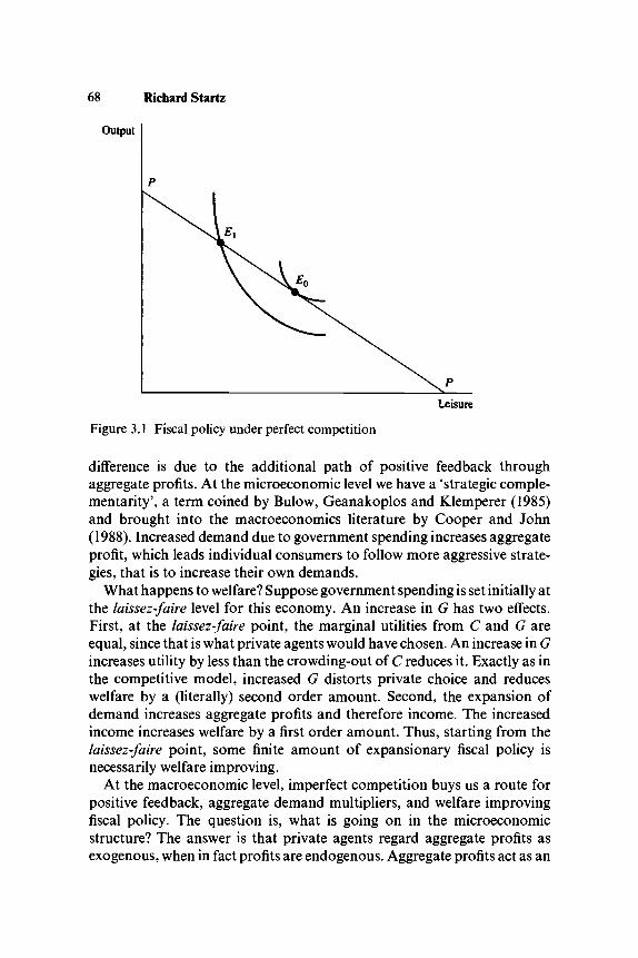
68 Richard Startz
Output
Leisure
Figure 3.1 Fiscal policy under perfect competition
difference is due to the additional path of positive feedback throughaggregate profits. At the microeconomic level we have a 'strategic comple-mentarity', a term coined by Bulow, Geanakoplos and Klemperer (1985)and brought into the macroeconomics literature by Cooper and John(1988). Increased demand due to government spending increases aggregateprofit, which leads individual consumers to follow more aggressive strate-gies, that is to increase their own demands.
What happens to welfare? Suppose government spending is set initially atthe laissez-faire level for this economy. An increase in G has two effects.First, at the laissez-faire point, the marginal utilities from C and G areequal, since that is what private agents would have chosen. An increase in Gincreases utility by less than the crowding-out of C reduces it. Exactly as inthe competitive model, increased G distorts private choice and reduceswelfare by a (literally) second order amount. Second, the expansion ofdemand increases aggregate profits and therefore income. The increasedincome increases welfare by a first order amount. Thus, starting from thelaissez-faire point, some finite amount of expansionary fiscal policy isnecessarily welfare improving.
At the macroeconomic level, imperfect competition buys us a route forpositive feedback, aggregate demand multipliers, and welfare improvingfiscal policy. The question is, what is going on in the microeconomicstructure? The answer is that private agents regard aggregate profits asexogenous, when in fact profits are endogenous. Aggregate profits act as an

Imperfect competition and New Keynesian economics 69
Output
Figure 3.2 Fiscal policy under imperfect competitionLeisure
externality. Atomistic decisions do not lead to a first best solution. This isan example of what we call a 'coordination failure'. It is not surprising thatsocial policy which moves the equilibrium closer to the first best is welfareimproving.
All this has a very 'macroeconomic' look. What might an intermediate-micro diagram look like? In figure 3.1, we show indifference curves betweenoutput (C and G combined) and leisure. Production exhibits constantmarginal product and takes place under a regime of perfect competition.The PP line is the production possibility set and coincides with theconsumer's budget line. Under laissez-faire, equilibrium is at Eo. Supposethe government introduces a lump sum tax and uses the revenue to transferG to agents. Equilibrium moves to a point like Ev (The budget line is nottangent to the indifference curve because the consumer is being forced totake more G and less leisure than she would choose privately.) While fiscalpolicy is expansionary, it is also, obviously, a bad idea.
In figure 3.2, the production function PP has constant marginal cost plusa fixed cost component. Because of the monopolistic mark-up, the con-sumer's budget line, BB, is more shallow than the production function.Assume that equilibrium is initially at zero profits and that this is reflectedin the height of the budget line. The consumer chooses point E2. The verticaldistance between Yx and Y2 is the producer's marginal profit, which is justenough to cover the fixed cost, leaving zero total profit. Suppose we repeatthe earlier exercise. The consumer, taking profits to be exogenous, 'initially'

70 Richard Startz
moves to E3.4 But at this point profits have risen because the BB line is flatterthan the PP line. As a result each consumer's budget line rises, furtherincreasing demand and thus further increasing profits. In general equili-brium, the budget line rises, say to something like BxBl9 a segment of whichis shown, and the economy moves to EA. (The income expansion path giventhe constrained goods/leisure choice runs through E3 and £4.) Not only isoutput up but, as drawn, so is welfare. This last result depends on thebalance between the leftward movement of E3 reducing welfare and theupward movement to E4 increasing welfare. (With Cobb-Douglas prefer-ences, it turns out that a small intervention is always good and a large one isalways bad.)
All this relied on the social production function, PP, not moving. So theanalysis given assumes away any changes in the strategic games played byproducers. As the most simple illustration of this limitation, the movementshown in figure 3.2 holds constant the number of firms even though in thepresence of fixed costs, average costs may be lower at EA than at E2. Since apoint like E4 has positive aggregate profits, the final long-run equilibriumought to involve some further movement of the PP curve. In Startz (1989),free entry increases the number of firms until the aggregate fixed costs arehigh enough to eliminate profits. In that model the movement of the PPcurve is just enough to return output to its prefiscal policy level.
The model as stated is really incomplete, because the productiontechnology and market structure are unspecified. A number of models usemonopolistic competition to support an increasing average returns to scaletechnology. With the Chamberlinian large numbers assumption, eachproducer takes her competitor's actions as fixed. The Dixit-Stiglitz modelmakes it particularly easy to compute the monopoly mark-up, as each firmfaces a constant elasticity demand curve. What is necessary at the microlevel is for there to be support for an aggregate positive feedback loop which'disappears' at the atomistic level. Monopolistic competition provides sucha structure, but it is not the only way to get there. Hart (1982) and others useCournot-Nash equilibria.
Aggregate demand and search equilibrium
Diamond (1982) and Diamond and Fudenberg (1989) produce a coordina-tion failure in a model of probabilistic search for trading partners. Agentscan enjoy the fruits of their labour only by exchanging their produce with atrading partner. The more likely an agent is to find a trading partner, thegreater the ex ante value of working. If more agents choose to work, thenany given agent is more likely to find a trading partner. Thus the decision to

Imperfect competition and New Keynesian economics 71
Figure 3.3 Strategic complementarity in Diamond's model
produce increases the probability of success for all other traders, acting inthis manner as an aggregate demand externality.
To illustrate, consider a much simplified variant of Diamond (1982).Each agent owns a coconut palm. Climbing the tree costs disutility c < 1. Ifthe tree is climbed, the agent harvests one coconut which is either sold,returning one util, or rots. The equilibrium probability of selling thecoconut is p. Maximizing expected utility, the agent climbs her tree if/? • 1 + (1 - /?) • 0 > c. Assume that c is distributed among agents uniformly onthe unit interval. The number of coconuts picked, y, is then p. (The first bestsolution is y = 1.) Think of this as giving the aggregate supply of coconuts.
Aggregate demand is written as the probability of finding a buyer as afunction of the number of agents searching, p(y). The function increasesmonotonically from/?(0) = 0, with the exact form depending on the searchtechnology. This is the source of strategic complementarity. Figure 3.3shows one possibility.
As drawn, there are several rational expectations equilibria, none ofwhich is a first best. The equilibria alternate between stable and unstable.To see this, suppose agents mistakenly believe that the probability of a saleis given by the point iO\ where aggregate supply is above aggregate demand.Producing at point'°' they will go to market and find too few buyers andtherefore will reduce output. The choice of equilibrium depends on anexogenous self-fulfilling prophecy as to the level of p. In other words, theeconomy can be moved from one static equilibrium to another byKeynesian 'animal spirits'.
Now add a government to the model which engages in taxes and

72 Richard Startz
Figure 3.4 Increase in aggregate demand
purchases, thus increasing the level of market activity at any level of output.Aggregate demand is increased, as shown in figure 3.4.
The stable equilibria move to higher levels of output. Since more outputis always better in this model, fiscal policy improves welfare as well asincreasing output.
The level of market activity acts as a public good and increasedgovernment provides more of it. One ought to ask why the government canprovide something private agents can not. In the previous section, fiscalpolicy distorted private choice so no individual agent would voluntarilyundertake the kinds of trades imposed by the government. In this section,we might assume some transaction cost of trading with the government.Every agent wants there to be expansionary fiscal policy in order to increasep, but no agent will voluntarily accept the transactions cost.
Imperfect markets enter in that no price clears the goods market - there isno auctioneer. (Monopolistic competition is not used in this model.) Thepositive feedback loop operates through increases in demand increasing theprobability of making a sale, which increases output and thus demand.Atomistic agents treat p as exogenous, even though p is endogenouslydetermined at the aggregate level.
Monopolistic competition and rigid prices
The greatest intellectual problem in macroeconomics is to understand therole of nominal prices. Economic theory is clear that only relative pricesmatter and use of a fiat numeraire is a mere bookkeeping convenience.5

Imperfect competition and New Keynesian economics 73
Most Keynesian economists, at least in the USA, believe that as anempirical matter changes in the real money supply move real GNP and thatin the short run nominal prices are rigid. The nominal money supply istherefore an effective tool to manage output.
The development of the menu cost literature as an underpinning for rigidnominal prices is the first serious theoretical development in this area. Theseminal works are Akerlof and Yellen (1985b), Blanchard and Kiyotaki(1987), Kiyotaki (1985) and Mankiw (1985). There is also a growingmodern body of work examining rigid prices per se (see Ball, Mankiw, andRomer, 1988, Rotemberg, 1987). Chapter 8 in Blanchard and Fischer'sLectures on Macroeconomics is devoted to this topic. Gordon's excellentsurvey in the Journal of Economic Literature (1990) 'sifts and criticizes' adecade's work in this area.
The best exposition of the menu cost literature is Mankiw (1985). Whatfollows is a variant of that model and of Blanchard and Kiyotaki (1987).Suppose all firms are price-setters, that aggregate demand depends on thereal money supply, and that a firm's market share depends on its pricerelative to the nominal price level. The profit function6 of the /th firm isni=n(Pi/P>M/p). Initially, there is some set of prices and correspondingquantity allocations which are privately optimal given the nominal moneysupply.
Suppose the nominal money supply is now increased A per cent. In theabsence of transaction costs, all nominal prices will rise by A per cent.Relative prices are the ratio of two nominal prices and therefore remainunchanged. The real money supply, profits, and quantity allocations will beas before.
Suppose instead there is a very small cost c to changing the nominal price,a 'menu cost'. If the gain from changing price is less than c, prices willremain at their initial levels. The gain from changing prices is dn/dpfKl+ A)pi—p i]/p. The initial optimum was found by setting dnldpt equal tozero, so for small A, d%ldpt is approximately zero. In other words, in theneighbourhood of the optimum, the rate of change in the objective functionis second order small. Even though menu costs are first order small, thepotential gain from changing prices is smaller and each firm will leave pricesfixed. As a result, relative prices remain unchanged, but the real moneysupply rises by A and aggregate demand increases. Further, if the level ofoutput was below first best, as is likely under imperfect competition, welfarerises.
The key insight is not that transaction prices might lead to sticky prices,but that very small transaction costs might lead to sticky prices. Imperfectcompetition is essential here. The more elastic the demand faced by firms,

74 Richard Startz
the greater the profit loss from having prices a given distance away from theoptimum. Under perfect competition, demand is infinitely elastic andtransaction costs will never cause sticky prices.
Aggregate demand and multiple equilibria
One form of early (pre-New) Keynesian theory created a set of equationswith multiple equilibria as solutions and suggested that economic fluctua-tions might be the economy's jumping from one equilibrium to another.Obviously one wants a theory that says more than that a set of non-linearequations has more than one solution. In particular, multiple solutions aremuch more interesting when they can be ranked (by a weak Paretocriterion, for example). One such theory is the 'sunspot' literature, in whichagents agree on some inherently irrelevant signal as a coordination device.Elements of the New Keynesian literature give aggregate demand a centralrole in coordination. It is natural to combine the question of coordinationwith imperfect competition. Perfect competition may result in multipleequilibria, but aggregate signals are irrelevant to atomistic perfect competi-tors once they have conditioned on the price vector. In contrast, imperfectcompetitors do care about quantities. The Diamond model discussed aboveis one example where aggregate demand matters to individual agents sothat changes in expectations of aggregate demand can move the economyfrom one equilibrium to another.
Kiyotaki (1988) presents a model of multiple expectational equilibriacentred around the investment sector. The production function exhibitsincreasing returns to scale. The role of monopolistic competition is tosupport an increasing returns to scale equilibrium. If firms are optimisticabout the future, they invest heavily now. The capital stock is large andtherefore output and demand are high, justifying the optimistic expec-tations. If instead, expectations are pessimistic, a low level equilibrium isreached.
Shleifer (1986) and Shleifer and Vishny (1988) present models whichspecifically emphasize aggregate demand spillovers. In Shleifer (1986),firms receive cost-reducing inventions at various times. However, they mayend up innovating, putting the inventions to work, in a coordinatedfashion. Innovation reveals the invention, which can be copied by otherfirms after a lag. To extract the maximum rent from the invention, firmswish to innovate during periods of temporarily high demand. Innovationitself raises demand. Shleifer demonstrates how endogenous cycles canresult.7
In Shleifer and Vishny (1988), each industrial sector has a high fixed cost/low marginal cost monopolist and a competitive fringe. If demand is low, it

Imperfect competition and New Keynesian economics 75
does not pay for the monopolist to operate. If demand is high, themonopolist produces. Since the monopolist has a high marginal product,aggregate output rises, calling forth monopolists in other sectors. Effec-tively, positive feedback operates through a market structure in whichsociety shifts to a higher production possibility frontier during good times.
In a slightly simplified version of the model, each consumer spendsy = n + L on each commodity, where n is aggregate profits and L isinelastically supplied labour. Fringe firms transmute one unit of labour intoone unit of output. The monopolist, if it operates, buys a cost-reducingtechnology at cost F which allows it to produce a > 1 units of output per unitof labour. The monopoly price is a scintilla under unity, capturing the entiremarket. The monopolist operates if its profit, n = y — y/<x — F, is positive.Suppose F is distributed according to H ( ) , which is uniform on [0,Hmax].Let F* be the breakeven cost. Equilibrium is defined by two equations inincome; the first defines the breakeven point; the second gives aggregatedemand.
• y 1
p* = y (breakeven)
y= I y — F\ dH( ) + L. (aggregate demand)
o
Together, the equations give the multiplier relation
dy _ 1dZ~ 1 /a - IV '1 J
The multiplier is greater than 1, but decreases monotonically as the size ofthe economy grows relative to costs of better technology (>>/Hmax). Notethat higher aggregate income is associated with more extensive imperfectcompetition and moving closer to the first best. The high fixed cost/lowmarginal cost technology assumed in this model does not permit compe-tition to support an efficient equilibrium.
The illustrative model here demonstrates positive feedback and has aunique equilibrium. The actual model in Shleifer and Vishny adds informa-tional considerations to produce multiple equilibria.
Related work
The primary work on abstract New Keynesian theory is Cooper and John(1988). The authors introduce the term 'strategic complementarity' to

76 Richard Startz
macroeconomics, emphasizing the importance of positive feedback, andgive examples using both game theory and imperfect competition. Weknow that for a single individual facing a competitive market there is a sensein which 'most' goods are substitutes rather than complements.8 Theauthors argue that understanding complementarity is central to under-standing the macroeconomy. Akerlof and Yellen (1985a, 1985b) serve asunderpinnings for the menu cost literature. In addition, the authors explainwhy small deviations from perfectly competitive behaviour on the part ofindividual agents can yield large and persisting deviations from the first bestat the aggregate level. While not yet greatly exploited in the literature, thismay provide a basis for a better understanding of inefficient business cyclefluctuations without requiring enormous departures from the competitiveparadigm. Finally, while not a New Keynesian model per se, the work byDe Long, et al. (1990), on 'noise traders', presents a related model ofpositive feedback in an efficient market.
Conclusions
The New Keynesian economics is too incomplete, and this is too incompletea review, to provide a final word on the literature. However, severalelements stand out. First, the New Keynesian economics is about thestrategic coordination of decision-making through aggregate demand. Forthis, perfect competition is a non-starter. Second, New Keynesians searchfor paths of positive feedback and strategic complementarity. Finally,imperfect competition in general and monopolistic competition specificallyare endemic in New Keynesian economics. However, the literature is toonew for there to be any agreement on how they should be used.
NotesThis chapter originated as background material for Robin Marris' ReconstructingKeynesian Economics with Imperfect Competition: A Desk-Top Simulation (1991).This version was revised for the University of Warwick Macroeconomics Work-shop (July 1993). I have benefited from discussion with Jean-Pascal Benassy, RussCooper, Huw Dixon, and others, but the usual disclaimer of assignation of blameapplies most strongly. The chapter is intended to give a personal view of the ongoingdevelopment of the 'New Keynesian economies'. The view is my own and I have notattempted to paint a picture shared by the profession as a whole. Because someimportant work is not discussed here, this is just not a valid literature review, butassuming the reader understands the context, I will proceed without furtherapology.1. Not all New Keynesians believe economic agents are rational, but agents ought
to be modelled as if they were. As a matter of history of thought, optimizing
Imperfect competition and New Keynesian economics 77
models drive out non-optimizing models. To quote Gordon (1990), 'Anyattempt to build a model based on irrational behaviour or submaximizingbehaviour is viewed as cheating'.
To be more careful, both New Keynesian and new classical economistssometimes consider carefully controlled departures from the economist's defini-tion of 'rationality'. Both groups are interested in topics such as 'boundedrationality' and 'adaptive learning' under uncertainty.
2. As a rule of thumb, the number of definitions of 'New Keynesian economics' isapproximately equal to the number of New Keynesian economists. (This rule ofthumb may sound circular, but is in fact resolved in general equilibrium.) Theterm 'New Keynesian' seems to have become a marketing rubric for ideas inopposition to the new classical school, rather than a single school centred aroundwhat Keynes said. The benefit of this is broad inclusion. The cost is that wemuddy the history of thought.
3. Gordon (1990) tells us: 'The task of new-Keynesian economics is to explain whychanges in the aggregate price level are sticky...' I emphasize here real, as well asnominal, models. If polled, I suspect the majority of macroeconomists wouldpick Gordon's definition.
4. Remember that there were no profits in figure 3.1, so the analysis ended here.5. The inflation rate is a relative price. But the serious disputes between classicals
and Keynesians lie in the failure of neutrality, not super-neutrality.6. Assume the function to obey any necessary regularity conditions, in particular,
to be differentiable in both its arguments. This is a substantive assumption, notjust one of convenience. Perfect competitors face infinitely elastic demand andtherefore their profit functions are not differentiable in their own-price.
7. Interestingly, stabilization policy can be harmful in such a model. If there arefixed costs of innovation, smoothing the business cycle may eliminate thetemporary rents needed to draw forth innovation.
8. Note also that proofs about the uniqueness of Arrow-Debreu equilibria passthrough much more easily if all goods are gross substitutes.


Part II
Goods market imperfections


4 Optimal labour contracts andimperfect competition: a frameworkfor analysis
Russell Cooper
Introduction
This chapter investigates the importance of labour market relations to themacroeconomic inefficiencies associated with imperfectly competitive pro-duct markets. Hart (1982) argues that models of imperfect competition arecapable of generating macroeconomic results such as an underemploymentequilibrium, multiplier effects and so forth.1 Related results on coordina-tion failures, i.e. the existence of Pareto ordered Nash equilibria, for thisclass of models are reported by Heller (1986), Kiyotaki (1988), Roberts(1987, 1988) and Cooper (1987).2
Some, but not all, of the studies on the macroeconomic implications ofimperfectly competitive product markets appear to rest on employmentrelations between firms and workers which are privately suboptimal. Forexample, Hart (1982) stresses the importance of market power by thesuppliers of labour in his study of imperfectly competitive economies.3 The'contracts' between workers and firms in Hart's model are not privatelyoptimal in that the allocation does not lie on a contract curve between thecontractants.
Another example of this point arises in Weitzman's (1983, 1985) studiesadvocating share contracts. Weitzman supposes that a 'wage system', inwhich the wage is predetermined and employment is demand determined,exists for the trading of labour services. He then contrasts the welfareproperties of this system with alternative compensation schemes assumingthat product markets are imperfectly competitive. Cooper (1988a) showsthat an imperfectly competitive economy with this structure of labourcontracts will generate underemployment equilibria and multiplier effectsusing a model similar to that of Hart (1982). That contracts such as theseproduce socially suboptimal behaviour is not surprising since these con-tracts are generally not even privately optimal. Hence, an important aspectof Weitzman's argument for the introduction of a share system appears to
81

82 Russell Cooper
rest on the assumption that agents trade labour services in a privatelysuboptimal fashion.
An important issue in this line of research is thus the role of labourmarkets in coordinating the activities of firms in the product market. Ifthere is an underemployment equilibrium, why are there no forces operat-ing in the labour markets to remedy the situation? Are the inefficiencies andother Keynesian features reported in these studies merely a consequence ofsome form of suboptimal labour arrangement which limits the coordina-tion of activities? To the extent that the implications of imperfect compe-tition reported are a consequence of the assumed contractual structure,imperfectly competitive product markets seem less important. As a conse-quence, this approach is subject to the criticism that the 'Keynesianfeatures' are simply a product of an arbitrary contracting structure.
There are two approaches to addressing this concern. First, one mightargue that these contracts are empirically relevant. Second, one can study amodel with imperfectly competitive product markets and privately optimallabour contracts. This chapter takes the second approach by introducingprivately optimal labour contracts into a simple general equilibrium modelof imperfect competition. The results indicate that economies with imper-fectly competitive product markets can experience underemploymentequilibria even in the presence of optimal labour contracts. In contrast toHart (1982), this underemployment reflects the product market power ofthe firm-union coalition and not the bargaining power of the union in itsrelationship with the firm. The framework can then be used to study thecomparative static properties of these models, as well as their policyimplications.
Overview of the model
Before delving into the details of the model, it is useful to begin with aninformal overview of the basic approach to this problem. The model hastwo key components. First is the design of a labour contract between agroup of workers and a firm. Second is the interaction of this coalition ofworkers and a firm with other such coalitions in the determination of aproduct market equilibrium.
Figure 4.1 displays the interactions between a single firm, the group ofworkers it contracts with and the product market in which it sells. Labourcontracts are negotiated prior to the determination of the state of theeconomy so that the maximal gains to risk sharing are possible. The state isfully described by the level of endowment of a non-produced good,preferences and technology.

Optimal labour contracts and imperfect competition 83
Figure 4.1 Interactions between the firm, its workers and its product market
Assume that both the firm and the workers costlessly observe the state sothat contingent compensation and employment rules are feasible. Note thatthe contractants negotiate both compensation and employment rulesrather than granting the firm the latitude to select employment expost givenwages. This is in keeping with the literature on optimal labour contracts.4Any inefficiencies in the equilibrium allocations will not be the consequenceof direct restrictions on the contracts. Following the specification of thelabour contracts, the random endowments, preferences and technology ofthe agents in the economy are determined and the product markets open.
The economy is composed of a number of sectors producing differentproducts. Demands in the economy are structured to highlight the specifi-city of production relative to consumption. In particular, workers and firmsare assumed to consume all products in the economy except for the outputthey produce. This structure of demands is common to models of coordina-tion failures and imperfect competition.5
In each sector, there are a small number of firms who act as oligopolists.The output of these firms is determined, on a state-contingent basis, in theirlabour contract. In designing this contract, the workers and the firmrecognize the market power of their coalition in the product markets. Inequilibrium, there is no incentive for a given worker-firm pair to changeoutput given the actions of other worker-firm coalitions.
The model of imperfect competition explored here has as a key featurethe underutilization of labour resources. As a consequence, increases indemand can be met by expanding output without the need to induceworkers to supply more labour by increasing real wages.6 In addition,wages do not decentralize employment decisions due to the presence ofoptimal labour contracts and prices do not decentralize product marketbehaviour because of imperfect competition. Evidence that wages andprices fluctuate little relative to quantities is consistent with this class ofmodels.
84 Russell Cooper
Structure of the economy and a characterization of equilibrium
Consider an economy composed of S sectors indexed by s = 1,2,..., S. Ineach sector there are F identical firms producing a homogeneous product.Firms in each of the S sectors produce a distinct commodity so that thereare S produced goods in the economy. There are TV workers per firm in eachsector who provide labour services to their respective firms. This allocationof workers to firms is not really a restriction given the symmetry in themodel. For simplicity we will often term a group of N workers, a union, andview contracts as negotiated between a union and a firm.
There is a non-produced good in the economy which is the endowment ofthe outsiders.1 These outsiders trade their endowments for the goodsproduced in each of the S sectors.
Preferences
In models of this genre, identical homothetic preferences are often used toavoid aggregation problems and distribution effects. These preferencesimply that demand curves are linear in income which eases the characteriza-tion of the Nash equilibrium in the product markets. We take a step furtherand assume that all workers and firms have Cobb-Douglas preferencesover the commodities they consume. This yields a closed form characteriza-tion of the equilibrium which is useful for expositional purposes andtractability.8 As noted above, agents do not consume the commodity theyare active in producing. Hence, workers and firms in sector s consume thegoods produced in the other sectors and the non-produced good. Relaxingthis assumption would lead firms to recognize that output expansionswould influence the position of their demand curves so that the underem-ployment effects would be weakened.
Workers in sector s have preferences given by
U(c.s,m,n)=U(nk^s(ckrm^-m) (1)where n equals one if the worker is employed and zero if the worker isunemployed and ck denotes consumption of the good produced in sector k.The consumption of the non-produced good is denoted by m. The disutilityof work equals r where 0 < r < l . Assume that (S— l)a + /?= 1, so thatpreferences are homothetic and that t / ( ) is strictly increasing and strictlyconcave so that workers are risk-averse. The demands generated by thesepreferences are
ct = {otlPi)Yfor zVs and m = PY (2)
where Fis the worker's income.
Optimal labour contracts and imperfect competition 85
Firms (i.e. a technology which is wholly owned by an agent in thiseconomy) in sector s spend the proceeds from their production activities oncommodities other than their output and the non-produced good. Firms'(shareholders') preferences are given by
V(c_s,m)=V(nk^s(ckrmp) (3)
where V{) is increasing and concave. Since firms and workers in the samesector have identical ordinal preferences, firms' demands are given by (2)with income equal to the profit level per firm, n. Firms' attitudes towardsrisk are characterized by V{).
The outsiders split their demands evenly across the S sectors andconsume the non-produced good as well. Their preferences are Cobb-Douglas with demands given by
ck= (*//>*Wf°r k= 1,2,...,5 and m= (1 -Sx)M (4)
where M is the aggregate endowment of the outsiders.
Technology
The presence of imperfect competition in product markets derives fromsome element in the industry which prevents the free entry and exit of firms.These barriers to entry are certainly important in understanding the long-run behaviour of a particular industry. Here, the model is very short-run innature so that these barriers will not be explicitly introduced into theanalysis. That is, we will simply assume that there are Ffirms per sector andnot model the source of this market power. An extension of this frameworkto study dynamics of entry and exit is provided in Chatterjee and Cooper(1989).
The technology will simply be a proportional relationship betweenoutput and labour input with one unit of labour producing 0 units ofoutput. Variations in (9, i.e. productivity shocks at the sectoral or aggregatelevel, can then be studied.
Assume that work sharing is not feasible so that workers are eitheremployed or unemployed. This may reflect features of technology whichmake hours and people imperfect substitutes. This structure is imposed sothat the model will generate employment fluctuations rather than varia-tions in hours, and allows us to investigate the role of unemploymentinsurance. See the related discussion in Hansen (1985).
Optimal labour contracts
We focus on the contracting problem between an arbitrary firm/of sector sand a group of N workers who form a union. The structure of unions and

86 Russell Cooper
the size of their membership is taken as exogenous for this exercise. Sincethe economy is symmetric, we focus on symmetric Nash equilibria. Thecontract devised for this firm and group of workers will therefore beoptimal for all other union-firm pairs in a symmetric equilibrium.
The exogenous variables, which are unknown to workers and firms whencontracts are negotiated, include: the endowments of the outsiders, (M),the preferences of the outsiders, (T), the preferences of the workers andfirms, (a, jS), and technology, (6). Denote by F the vector of these para-meters describing the state of the economy. In addition to the variablesincluded in T, payoffs to the worker-firm coalition depend on the ex postquantity decisions of other coalitions in the economy. These variables areconjectured, on a state-by-state basis, by the contractants when negotiatinga contract ex ante. In equilibrium, these conjectures are correct. So a labourcontract will be written contingent on the realization of the randomvariables in the economy, given conjectures about the ex post quantitydecisions of other coalitions in the economy. All expectations used indescribing the contracting problem will be relative to the distribution of F9which is common knowledge.
The optimal contract between firm/of sector s and that firm's N workersis characterized by three schedules: we(T), w"(T), and L(F). The firstschedule is the state-contingent wage paid to employed workers, the secondis the state-contingent level of severance pay and the third is the employ-ment rule contingent on F as well. To simplify notation, denote a contractby S and eliminate the superscripts and subscripts. The union-firm choose 3to maximize
E{V(zn) + a[(L/N)U(zwe - r)+ (N~ L/N)U(zwu)]} (5)
subj to: L(F)<N and
we,wu,L non-negative for all F.
In the objective function, a represents the bargaining weight attached toworkers' expected utility. The ratio LIN is the probability that a givenworker is employed if L workers are employed under the optimal contractin some state. The firm's utility function depends on the product of thefirm's profit n and a variable z (which is defined below and also appears inthe workers' payoffs). The profit level is
n = R{L,F)~ weL -wu(N- L). (6)
The function R(L, F) is the firm's revenue if it employs L workers in state F.The variable z appears in the payoffs of both the firm and the workers and
is a price deflator for the market basket of goods generated by the Cobb-Douglas preferences. For later reference,
Optimal labour contracts and imperfect competition 87
(*ipky. (7)Assuming for the moment that the constraint on the employment level
not exceeding N does not bind, the first order conditions for the problemcan be summarized by
U'(wez-r)a/N= U'(wuz)a/N= V'(zn) and (8)RL(L,F) = r/z for MF (9)
where RL is the derivative of R(L,F) with respect to L?(8) implies that risks are shared efficiently between the firm and its
workers. Because of the strict concavity of U( •), (8) implies that workers areindifferent between the states of employment and unemployment, i.e. thelevel of severance pay compensates the unemployed worker for the lostwage income less the utility of leisure (r). As a consequence, workers'welfare is independent of employment status. Note though that as long asthe firm is not risk-neutral, the utility level of workers will depend on thelevel of economic activity in the economy.
(9) represents the employment rule in the optimal contract. Since workersare indifferent between employment and unemployment, the only cost tothe firm of employing an additional worker is the value of that worker'sleisure in terms of the consumer basket, r/z. The gain to employing anotherworker is the marginal revenue gained from selling an extra unit of output.If the constraint that L < N binds, then employment is set at N and (9) doesnot hold with equality.
The important element about (9) is that once F is determined, thisexpression determines the firm's action in the ex post product market game.The union and the firm act as a coalition in this product market game withtheir strategy determined in the ex ante labour contract. In contrast to Hart(1982), the employment decision reflects the joint market power of theunion-firm coalition in product markets and not the labour market powerof the union per se. That is, the employment rule is independent of a. Thereare no pressures to force the economy to full employment: the optimalcontract allows some workers to remain unemployed as a means ofobtaining the largest surplus possible given the market power of the firm.
Of course, the level of wages does depend on o as this parameterdetermines how the surplus from the market game will be shared. Thisseparation of employment and compensation arises from the structure ofpreferences (i.e. no income effects) for the contractants.10 The decisions ofthe union-firm in the product market game are thus equivalent to that of afirm facing a marginal cost of labour (in terms of the numeraire) of r/z.
(8) and (9) completely specify the employment, wage and severance payschedules in an optimal contract between firm / in sector s and its N

88 Russell Cooper
workers. Recall that we have omitted any notation regarding the identity ofthis firm or its sector of operation. Given the symmetry of the problem, theconditions describing this optimal contract also characterize that for otherunion-firm pairs in other sectors. The only change that is necessary is todefine z to correspond to the sector of interest. Given this optimal contract,we are able to compute the Nash equilibrium in the product market.
Goods market equilibrium
To complete our characterization of an equilibrium, we need to model theinteraction of firms in product markets, ex post. We will concentrate onsymmetric Nash equilibria for this economy. The labour contracts nego-tiated ex ante with their unions, specify an employment rule for a firmcontingent on the realization of random variables in the economy. Theinteractions of these employment rules will then determine the equilibrium.The revenues earned by firm / o f sector s are:
R(Lir)=psq{=(EJQs)q{ (10)
where q{= L{6 for a l l / and Qs is the total output in sector s.The Cobb-Douglas preferences imply that each commodity has a
constant budget share for each of the consuming agents in this economy.Hence, the price in sector s is simply the total expenditure in that sector, Es,divided by the total output in sector s, Qs.
Denote by qs the level of output for each firm in sector s if they are allproducing at the same level. Since the expenditure on sector s is indepen-dent of qs, we can solve for the symmetric partial equilibrium in sector s byfinding that level of output per firm in that sector which is a best response tothe output levels chosen by the other firms in that sector given the level ofexpenditure on that sector. To do so, use (10) to solve (9) yielding
rlzs (11)
where r\ is defined as (l — l/F). Note that (11) holds only when theconstraint that L<Nis not binding.11 The variable rj will serve as a usefulmeasure of the market power of firms in the economy. As F-> oo, rj-> 1 whilerj-*O as the industry approaches monopoly. Recall that the sectors aresymmetric so that rj is not indexed by the sector. Using (11), the price insector s is simply
ps = r/(rjdzs). (12)
It is important to note that z depends on prices in other sectors as well asparameters of preferences so that, in (11) and (12), we index it by s.
To characterize the symmetric Nash equilibrium for this economy, note
Optimal labour contracts and imperfect competition 89
that (11) and (12) hold for all s. Since zs depends on the prices in othersectors, we can solve for the output price, common to all sectors, using (7).This will be
p=(rMe)l/fi/^l-^p (13)
where 6 is a productivity shock (assumed for now to be) common acrossfirms and sectors. Note that prices can be determined independent ofoutput levels as long as L<N. This is a feature of homothetic preferencesand constant marginal costs. This implies that variations in the endow-ments of outsiders will cause output but not prices to change.
To determine the output level of an arbitrary firm in sector s (given thatall firms are producing the same level of output in the partial Nashequilibrium), we need to specify the level of expenditure on sector s. Usingthe Cobb-Douglas preferences, this is given by
E^aFZ^sP^ + xM. (14)
Again note that the summation here is over sectors other than s. Using (12),in a symmetric Nash equilibrium, (14) can be rewritten as
E=Fp[*Zk*Ak + x*M] (15)
where <P=\/Fp = Orjz/Fr.This expression implies that the total expenditure on sector s depends on
the level of economic activity in all the other sectors and is proportional tothe endowment of the outsiders. This is similar to a simple model of incomedetermination in which there are autonomous expenditures and an expen-diture term which depends on the level of economic activity.
Inserting (15) into (11) implies
qs = aZk^sqk + T&M= aZk^sqk + xMIFp. (16)
So the per firm level of output in sector s is a linear function of the aggregatelevel of activity in other sectors and the per firm endowments of theoutsiders (in terms of the produced commodity). For S large enough (sothat each sector is small), (16) implies that the level of output per firm insector s is a linear function of the aggregate output level in the economy.
Figure 4.2 displays a 'reaction curve' for sector s for a given level ofactivity in other sectors. Note that this is not literally a 'reaction curve' for aparticular firm but rather an expression for the sector-specific Nashequilibrium output level for given output levels of other firms. The interceptof this 'reaction curve' is the sector-specific level of autonomousexpenditures.
As the output levels in other sectors increase, all of the firms in sector swill expand as well. So even though the firms in a given sector are producing

90 Russell Cooper
A = xMIFp
Sector s 'reaction curve*
Slope = a < 1
Figure 4.2 A reaction curve for sector s
perfect substitutes, positive interactions (strategic complementarities) arepresent between firms across sectors in a symmetric Nash equilibrium.
Since (16) holds for all s, we can use it to compute the output level per firmin each sector in a symmetric Nash equilibrium. This output level is given by
zM/Fp\-(S-\)a~ (17)
where A is the level of autonomous expenditure on the produced good.Recall that /? is the budget share of the numeraire good and represents theshare of income that leaks out of the income stream connecting the firms inthe economy.
To guarantee that this level of output is feasible, we need to check thatq<N0 since each firm had available only N workers. This inequality issatisfied as long as M is not too large and p not too small. We will use (17) asan equation for the equilibrium level of output even though it contains theprice in it. From (13), we know that the equilibrium price level isindependent of output.
When the level of output given in (17) exceeds ON, then the economy is atfull employment and the expressions derived in this section will not apply.Each firm will then simply employ all TV workers and prices in each sectorwill adjust so that markets clear at full employment.
Finally, and perhaps most importantly, note that the equilibrium levelsof output, employment and prices are actually independent of a number oflabour market variables in this economy: the number of workers N and the
Optimal labour contracts and imperfect competition 91
bargaining weight a. This independence of the equilibrium of the number ofworkers is also a property of many efficiency wage models (see, for exampleWeiss, 1980 and Yellen, 1984). If the level of per firm output satisfying (17)is less than N, we have an underemployment equilibrium. Furthermore,increasing the number of workers in this economy (assuming that they alljoin a union) will only increase the unemployment rate and will not alter theform of the optimal contract between the union and the firm. Again, theoptimal contract specifies employment to obtain the maximal amount ofpayoffs for the coalition of workers and the firm, and this decision rule isindependent of the number of workers N and the bargaining weight. Thiseconomy therefore has the property that there are no forces at work toreduce the rate of unemployment since the agents in the economy have noincentive to employ the excess labour force.
Overall, the equilibrium for this economy is quite similar to thatdescribed by Hart and others, although here the labour relations are theconsequence of a privately optimal contract. Hart (1982) provides adiscussion of multiplier effects and the presence of a balanced budgetmultiplier for his economy. Those types of comparative static results can beobtained for this economy as well.12 (17) can be used directly to evaluate theeffects of variations in M as long as the economy operates in an underem-ployment region. (13) and (17) can be used to evaluate the effects of changesin aggregate productivity.13 Moreover, though this economy had a uniqueequilibrium, it is possible to construct economies with multiple equilibria,along the lines of Heller (1986) and/or Kiyotaki (1988), in which labourservices are traded with labour contracts. We thus see that the mainconclusions of the previous work on the implications of imperfect compe-tition are robust to the introduction of privately optimal labour contracts.
Conclusions
The goal of this chapter has been to provide a framework of analysis forcoordination failures in imperfectly competitive economies. In contrast toother studies this area, this chapter includes a representation of labourmarkets through a contracting framework. This approach provides someperspective on the manner in which adjustments in the labour marketinfluence the operation of product markets. To the extent that labourcontracts bind workers and firms into a coalition that seeks to gain its shareof surplus, there are no forces at work in labour markets to move theeconomy towards an efficient outcome. The model can then be used in astraightforward manner to derive some comparative static properties ofimperfectly competitive economies and to conduct some policyexperiments.

92 Russell Cooper
This framework is intended as a basis for other research on theimplications of macroeconomic imperfect competition.14 One can amendthe model to study a number of dynamic issues such as the role of entry andexit. Further, the contracting problem can be made more interesting byintroducing asymmetric information, and the aggregate implications of thisdistortion can be investigated.15 Finally, the framework may be useful instudying the interaction between the organization of labour relations (forexample, the nature and extent of unionization) and aggregate behaviour.
Notes
This is a revised version of Cooper (1986). Much of this research was conductedwhile I was a Visiting Scholar at the Board of Governors of the Federal ReserveSystem. I am very grateful to that institution for its support. Seminar participants atthe 1986 NBER Summer Institute, the University of Delaware, the University ofIowa, the University of Pennsylvania, the University of Western Ontario and the1987 NBER Conference on Labor Markets and the Macroeconomy providednumerous helpful comments and suggestions. Dale Mortensen provided an excel-lent presentation of the original paper at the 1987 NBER Conference on LaborMarkets and the Macroeconomy which helped considerably in this revision.Comments from Robin Boadway, Randy Wright, Jon Strand and Peter Howitt andtwo anonymous referees are also appreciated. Financial support from the NationalScience Foundation, NSF No. SES86-05302, is gratefully acknowledged. Thischapter previously appeared in the Canadian Journal of Economics (1990), pp. 509-22, and we would like to thank Toronto University Press for their kind permissionto reproduce it here.
1. Related results on multipliers in similar models are reported by Startz (1989)and Mankiw (1988). The term 'underemployment equilibrium' refers to thepossibility that labour may not be fully employed in equilibrium. This is notnecessarily an inefficient outcome as it could arise in an Arrow-Debreueconomy as well. However, underemployment equilibria are more likely toarise in models with imperfect competition.
2. Cooper and John (1988) discusses the relation of these results to othercoordination models associated with trading externalities (Diamond, 1982 andHowitt, 1985) and production externalities (Bryant, 1983).
3. Hart (1982) notes that these results are also dependent on the inelastic laboursupply of workers. Dixon (1987, 1988) adopts a similar model of unionbehaviour.
4. For a review of that literature, see Cooper (1987) and Rosen (1986).5. See, for example, Cooper and John (1988) and Heller (1986).6. This implication of imperfect competition is exploited by Hall (1987) and
Cooper and Haltiwanger (1990) as well.7. In dynamic models of imperfect competition, this outside good is often treated
as fiat money. See, for example, Chatterjee and Cooper (1989).

Optimal labour contracts and imperfect competition 93
8. An earlier version of this chapter described the implications of relaxing thesestrong assumptions.
9. These conditions are obtained by differentiating (5) on a state-by-state basissince there are no terms involving the rate of change in the state F.
10. If there were income effects and employment was not {0,1}, then market powerwould influence the level of employment through the disutility of work. In thiscase, the results would be quite sensitive to the specification of preferences. Inaddition, this specification implies that workers are indifferent between beingemployed and unemployed.
11. When L = N, the economy is at full employment and prices must vary to clearmarkets.
12. See Cooper (1986) for a characterization of these comparative statics.13. Sector-specific productivity shocks can be shown to lead to economy wide
fluctuations through changes in relative prices, see Cooper (1986).14. Cooper (1986) spells out these applications in more detail.15. See Kahn and Mookerjee (1988) for work in this direction.

5 Market power, coordination failuresand endogenous fluctuations
Claude d'Aspremont, Rodolphe Dos Santos Ferreiraand Louis-Andre Gerard- Varet
Introduction
Imperfect competition has become one of the main ingredients of theso-called 'New Keynesian economics'.1 Much recent work has emphasizedKeynesian features of imperfectly competitive macroeconomic models,2belonging either to the Cournotian tradition, as in Hart (1982), or to one ofthe monopolistic competition brands, corresponding to the Chamberlinianframework of Dixit and Stiglitz (1977) (Weitzman, 1985; Blanchard andKiyotaki, 1987), or to Hotelling's spatial model (Weitzman, 1982). Asomewhat paradoxical aspect of part of this literature is that it actuallyappears quite unkeynesian, not so much because Keynes himself paid littleattention to imperfect competition, but essentially because some of itsresults, concerning in particular unemployment or the response to aggre-gate demand shocks, depend either on union power,3 or on small adjust-ment costs ('menu costs')4 and 'nearly rational' behaviour of price-settingagents,5 and thus in a sense come back to 'classical' explanations, in terms ofwage and price rigidities or frictional phenomena.
We do not want to deny the relevance of such explanations. We proposeto explore in this chapter only some consequences of firms' monopolypower, in a context of full rationality, complete price flexibility, withoutadjustment costs and in the absence of exogenous shocks. Since we conformto the Keynesian priority given to the product market relatively to thelabour market, and since it is the output market power that we want toemphasize, we shall (unrealistically) assume perfect competition in ahomogeneous labour market. And, as an attempt to unify the theoreticalframework, facilitating comparisons, we shall use a model of 'Cournotianmonopolistic competition',6 which generalizes and extends both the Cour-notian and the Chamberlinian approaches to imperfect competition. Themodel involves several goods, each produced by several firms, and includespure Cournot oligopoly and pure monopolistic competition as particularcases. When making a decision, the producer of a good is supposed to take
94

Market power, coordination failures and endogenous fluctuations 95
as given the total quantity of that good produced by other firms and theprices of the other goods, while knowing the 'objective' demand, that is,acting on the basis of rational conjectures about consumers' behaviour.
The model further extends early imperfectly competitive models byassuming overlapping generations of consumers. This is of course aconvenient step towards the dynamic analysis of intertemporal equilibria,involving in particular the study of the conditions in which endogenousfluctuations occur. Besides, coexistence of two generations of young andold consumers allows us to incorporate not only individual income andsubstitution effects on the demand elasticity, and hence on the firms' marketpower (and the case where the former dominates the latter, the complemen-tarity case, will turn out to be interesting), but also redistributional effects,between the young and the old. Such effects may account for a significantvariability of such market power, induced by changes in demand elasticityas the output price varies.
It is this variability, more than the existence of a strong market power initself, that drives interesting effects.7 Indeed, alone or in conjunction withdecreasing marginal cost8 (compatible with equilibrium because of imper-fect competition), mark-up variability may be responsible for a reversal ofthe slope of the adequately defined 'oligopolistic labour demand' curve.This reversal, by having that curve cut the labour supply curve more thanonce, can naturally lead to a multiplicity of temporary equilibria in thismodel where, on the contrary, a unique equilibrium would have resultedfrom non-increasing returns together with weak mark-up variability (asunder nearly competitive conditions or under substitutability). Multipletemporary equilibria, corresponding to different employment levels, mayeven be Pareto-ranked, giving rise to a situation of 'coordination failure'9which cannot occur under perfect competition (as we well know from theFirst Fundamental Theorem of Welfare Economics).
The same factors, increasing returns and variability of market power,that account for a multiplicity of temporary equilibria, also favour,through their influence on the form and movements of the oligopolisticlabour demand curve, emergence of endogenous fluctuations. Givenenough complementarity, such fluctuations can occur in a perfectly compe-titive world.10 But we will show that if, in an extreme form of market powervariability, marginal revenue becomes negative11 when prices are notexpected to change much in the next period (a condition which excludes theexistence of a stationary equilibrium), and if returns are increasing (acondition that further excludes in our model the existence of a monotonicequilibrium), then all equilibria are characterized by persistent endogenousfluctuations in prices and output.
The chapter is organized as follows. In the second section we describe the

96 Claude d'Aspremont et al
model of Cournotian monopolistic competition and define the equilibriumconcepts that we will use. The third section exhibits a multiplicity of Paretoranked (temporary or stationary) equilibria, under increasing returns orunder significantly variable market power. More complex intertemporalequilibria, generating endogenous fluctuations, are analysed in the fourthsection. We then conclude.
The model
We use an overlapping-generations model in discrete time. In each periodr = 0,1,2,..., there are ra + 2 commodities: m produced goods (ra>2),labour and money, which is both the unit of account and the only storablegood. The economy is endowed with a constant stock of money M.
We consider two types of agents: consumers and firms. Each consumerlives for two periods, works and earns income when young, but consumesthe produced goods both when old and when young. At each period and forevery good k= l,...,m, there are n firms producing good k. The labourmarket is assumed competitive. However, in the produced good markets weassume Cournotian monopolistic competition, in the sense that each pro-ducer of good k maximizes his profit, facing the 'true' demand for good k,net of the total quantity produced by the others and given the prices of theother produced goods.12 In this section we shall first derive the demandfunctions from consumers' behaviour, then present the firm's problem andintroduce both a temporary and an intertemporal concept of Cournotianmonopolistic competition equilibrium. Finally we compare our model toothers in the literature.
Consumers' behaviour and demand functions
In each period t= — 1,0,1,..., a continuum of consumers of mass L is born.Each individual lives for two periods and receives, while young, an income(profit or wage). Preferences of young consumers, identical for all indivi-duals, are homothetic and separable, represented by the function
U[u(c)M£)]~vl, (1)where c e &™ and c e &™ denote respectively present and future consump-tion baskets, /e{0,l} is an (indivisible) labour supply and v is the (non-negative) disutility of work. The function U is twice-differentiable, stronglyquasi-concave, increasing, homogeneous of degree one, and such that theindifference curves do not cut the axes. The function u is a symmetric CESfunction. We assume that the preferences of old consumers are representedby this same function u.

Market power, coordination failures and endogenous fluctuations 97
Consumers know and take as given the current prices/? e 0tm+ + and, whenyoung and hence in the labour market, the current wage w e ^ + . Also,young consumers are assumed to have identical rigid point expectationsabout future prices p e $"l +.
Separability of preferences entails the following convenient procedurefor utility maximization of the young consumer:
1. Optimal consumption baskets are first chosen for each period,assuming given expenditure levels. Let
( \s/(s-\)
-lctl)/s) = C9 (2)mk=\ )where se$+ + \{\} is the elasticity of intersectoral substitution.13 Notice
that the CES function u can be seen as defining an index for totalconsumption C, since the expression for C/m in (2) is just a mean of thequantities in the consumption basket. If the mean price is defined by theformula
( 1 m \ 1/(1-5)
»1Hthen c£, the A:th element of the optimal consumption basket for anexpenditure x in the first period of consumer's life, can be expressed as
so that YjPkct^PC = x' Clearly, similar expressions hold for the optimalk
consumption of an old consumer as well as for c£ the future consumption ofa young consumer (as a function of the future price/^ and the future meanprice P).
2. An optimal intertemporal consumption decision is then taken, given atotal income /. By homogeneity of the function U, we get
C* = h(P/P)i/P and C* = [1 - (P/P)h(P/P)]i/P, (5)
where h is a twice-differentiable, decreasing function. We shall hence-forward denote:
6 = P/P the real interest factor, anda(0) = 6h(6) the propensity to consume.
Notice that O<a(0)< 1, since the indifference curves of U do not cut theaxes. The optimal intertemporal consumption structure

98 Claude d'Aspremont et al
C* h(d) OL(0)
C* 1-0A(0) 0 l -(6)
is a twice-differentiable, decreasing function of the real interest factor. Weshall denote:
a(6)= -H'(9)6/H(6) the elasticity of intertemporal substitution.A simple calculation shows that a(6) = 1 - (a'(0)0)/(a(0)[l - a(0)]), so thata is increasing (resp. decreasing) in the case of intertemporal complemen-tarity, i.e. if G< 1 (resp. substitutability, i.e. if a> 1). The utility derivedfrom optimal consumption
U(C*9 C*) = tf (a(0), 0[1 - a(0)])i/P= U*(0)i/P (?)is linear in the real income i/P and increasing in the real interest factor 6.Indeed, using the first order condition U\ = U'2O, and Euler's identityU= U\*+ U'2e(\ - a ) , we have:
U*'g= (U[- U'28)(x'e+ Uf26(\-(x)=U*(l-(x)>0. (8)
3. Finally, the consumer chooses to work (resp. not to work) if U* (6)w/P- v > 0 (resp. < 0). Indifference prevails in the case of an equality. Thus,
is the real reservation wage, equal to the ratio of labour disutility to utilityof optimal consumption.
Since demand is the same linear function of income for all youngconsumers, income distribution is immaterial (notice that we do not assumethat shares of firms are uniformly distributed), so that aggregate demandby the young is a linear function of aggregate income /. In the same way, thedistribution of cash balances among the old is also immaterial, and theiraggregate demand is a linear function of the money stock M. Moreprecisely, first notice that the aggregate expenditure Xis given by the sum ofthe money stock, which is completely spent by the old, and of the aggregateincome multiplied by the propensity to consume, corresponding to what theyoung spend:
X=a(PIP)I+M. (10)Thus, as / = Z i n equilibrium, we obtain the following expression for theaggregate demand:

Market power, coordination failures and endogenous fluctuations 99
which is the familiar product of the Keynesian multiplier and the auton-omous demand. Since demand has the same structure for all consumers,whether young or old, given by (4), we then get the sectoral demand forgood k:
p^) = -iP-i\ SD(P9P). (12)
By symmetry, the function d is the same for all produced goods, so that anindex k is not required.
If we now refer to the elasticity of aggregate demand D(,P):
dD P
and using:d^p,dpkP' m\Py
we can easily compute the elasticity of sectoral demand for good k:d
Hence, the sectoral demand elasticity S appears as a weighted average of theelasticity of intersectoral substitution s and of the aggregate demandelasticity A, itself a weighted average of the elasticity of intertemporalsubstitution a and of unity (corresponding to the spending behaviour of theyoung and the old, respectively). It is necessarily positive.
Producers' behaviour
Every good k = 1,..., m is produced by the same number n of firms (n > 1),with identical increasing, but not necessarily convex, isoelastic cost func-tions: y^ (with /? > 0), giving the labour quantity required by output y.
Each producer/ of good k takes as given the wage w in the labour market,while acting as a Cournot oligopolist in the market for the produced good k,on the basis of the 'true' residual demand for his output, contingent on thesupply of the other firms in the same sector:
d{Pk,P(Pk,p_klP)- Yk_p with Yij^Zvtf.

100 Claude d' Aspremont et al
We assume that producer j knows the common mean price expectation P,and conjectures (correctly at equilibrium) the vector p_k of other commod-ity prices and the output Y_j of good k produced by the other firms. Theseconjectures are essential for our notion of Cournotian monopolisticcompetition. The function d(.,P(.9p_k),P) being strictly decreasing inpk,we may introduce the inverse demand function xj/ for the output of firm j ,which is:
_k)J)- Yk_j. (16)Then, for any given Y,p, P and w, the typical 'producer's problem' is the
following profit maximization problem:
max 7r(x) = max *A(.y + Y,p,P)y — wyp (17)
(for simplicity of notation, we omit the indices y and k). An optimal positiveoutput y must satisfy the first order condition (with ij/(y) standing for
which is the familiar equality of marginal revenue and marginal cost. Itmust also entail a non-negative profit: ij/(y)y>wyp (otherwise it would bedominated by a zero output), so that (using (18)):
Lemma 1 and Lemma 2 in the appendix introduce restrictions (on thefunction E and on the elasticity 8 of sectoral demand, respectively), ensuringthat the ratio of marginal revenue to marginal cost is decreasing whenevercondition (19) is verified and the marginal revenue is non-negative. Thenconditions (18) and (19) are sufficient for a global maximum of the profitfunction (unique in the positive domain), although that function may fail tobe quasi-concave. Based on these lemmata, the following propositions givesimple assumptions on s and a implying that the first order conditiontogether with the non-negative profit condition are necessary and sufficientfor profit maximization at a positive level of output. We stick to two typicalcases: overall (both intertemporal and intersectoral) complementarity andoverall substitutability.
Proposition 1 (complementarity): Assume intersectoral comple-mentarity: s< 1. Also, assume that the elasticity of intertemporal substitu-tion a satisfies, for any 6e$+ +,

Market power, coordination failures and endogenous fluctuations 101
(T(6)< 1 and °^> ~ [1 ~(7(9)] (20)a(U)
or, equivalently, that the intertemporal expenditure structure 6H(6) is anincreasing and concave function of 6. Then, the first order and non-negativevalue condition:
wherep = \j/(y+ Y,p,P)as defined in (16), is necessary and sufficient for y tobe the unique positive solution to the producer's problem (17).
Proof: See appendix.
Proposition 2 (substitutability): Assume intersectoral substitut-ability: s > 1. Also, assume that the elasticity of intertemporal substitution asatisfies, for any 6 e 01+ +,
I <(j(6)<min{s,l + p} and a'(6)>0. (22)
Then, the first order and non-negative value condition (21) is necessary andsufficient for y to be the unique positive solution to the producer's problem(17) ( Y>0 and hence n> 1, is required in condition (21) if 5= 1).
Proof: See appendix.
Temporary and intertemporal Cournotian monopolistic competitionequilibria
Two concepts of equilibrium are successively considered: temporary andintertemporal equilibrium. Temporary equilibrium imposes compatibilityof optimal consumers' and producers' decisions in the particular periodwhich is considered, but price expectations remain exogenous and arearbitrarily given:
Definition 1 (temporary equilibrium): A temporary equilibriumassociated with the expected mean price P is a vector with componentsy*j>0 (the outputs chosen by each firm j=l,...,n in each sector k= l , . . . ,m), p*>0 (the product prices, with k= l , . . . ,m), and w*>0 (thewage), such that:
1. for any firm j in any sector k,
max ifr (y + Ya y*i>P^/o P) y ~ w*y^

102 Claude d'Aspremont et al.
with the sectoral inverse demand function \\i as defined in (16),2. for any sector k, £ y%= di<P* p*> ?)> w i t h P* = p(P*>P-k)>
j3- Z Z y*f = L and w*/P> v/U*(P*/P) (full employment) or
f and w*/P= v/U*(P*/P) (underemployment).
Conditions 1 and 2 characterize a Cournotian monopolistic competitionequilibrium in the product markets: every producer maximizes his profit,knowing the 'true' consumers' demand function and their expectation ofthe mean price in the next period, acting as a Cournot oligopolist in his ownmarket, and taking as given the wage and the other products prices.Condition 3 defines the competitive equilibrium of the labour market by theequality of supply and demand, but taking into account the possibility thatonly part of the labour force is employed. In this case, since we assumeperfect wage flexibility and no rationing, the wage must be equal to itsreservation value.
It can be checked that all equilibria are necessarily symmetric inquantities, inside each sector, relatively to active firms (see Lemma 3 in theappendix). But the possibility that only a number n* <n of firms be active inequilibrium cannot be excluded when returns are increasing (/?< 1). Also,symmetry is not always warranted in prices, and correspondingly inquantities across sectors, unless we strengthen the assumptions hithertoformulated.14 For simplicity we shall however simply ignore asymmetricequilibria, and the kind of multiplicity they may introduce.
It will be appropriate to refer to a symmetric temporary equilibrium by atriplet (y*,p*, w*) characterized, under the assumptions of either Proposi-tion 1 or Proposition 2, by:
1. the first order and non-negative value condition:
w * / ^ ~ ' ( 2 3 )
with S as given by (15) and (13),2. the product market equilibrium condition:
1 M( 2 4 )
3. and the labour market equilibrium condition:
mny*p = L and w*/p*>v/U*(p*/P) (full employment)or mny*^<L and w*/p* = v/U*(p*/P) (underemployment)

Market power, coordination failures and endogenous fluctuations 103
The characterization of symmetric temporary equilibria can be furthersimplified by referring to just the equilibrium price p*9 which may bedetermined using workers' and firms' reservation wages. Let us first definethe symmetric marginal revenue function
( 2 6 )
such that 1 — p(p;P)/p = l/nd(\,p/P) is Lerner's index of monopoly power.Then the firms' reservation wage15 is constructed from the first ordercondition (23) and is equal to the product of the marginal productivity bythe marginal revenue. In a symmetric product market equilibrium, usingcondition (24), this is simply the following function of the price p (con-ditional on a given price expectation P)\
a}'ip;P)=~B(~^T) p{p;Py (27)
The function cof has elasticity:
"("7P- (28)
Similarly the workers' (nominal) reservation wage is constructed from(25) as a function of the same variables:
( 2 9 )
with elasticity (for v>0, and using (8)):
°^ (30)
The following proposition summarizes all the simplifications comingfrom symmetry:
Proposition 3 (symmetric temporary equilibria): An underemploy-ment symmetric equilibrium is determined by equalizing both reservationwages, and verifying that a solution p* to the equation cOf(p;P) = cDt (p',P)satisfies:
L>(mny~pD(p*,PY and Pp*>p(p*;P). (31)
A full employment symmetric equilibrium is given by the solutionp** to theequation L= {mn)l~^D (/?**,/>/, whenever this solution satisfies:

104 Claude d'Aspremont et al.
tp**^) and Pp**>p(p**;P). (32)
We finally give the definition of an intertemporal equilibrium which, inaddition to the compatibility of optimal consumers' and producers'decisions in every period, imposes the fulfilment of price expectations.
Definition 2 (intertemporal equilibrium): An intertemporal equili-brium is a sequence of temporary equilibria, one for each periodt = 0,1,2,..., associated with an expected mean price Pn characterized by amean price Pf and such that, for any
Clearly, as we restrict ourselves to symmetric equilibria, an intertemporalequilibrium is completely described by a sequence of triplets(y*>P**w*)tejr- As suggested by the simplified characterization of sym-metric temporary equilibrium given in Proposition 3, a symmetric intertem-poral equilibrium can also be simply identified to a sequence of positiveprices (p*)tBjr.
Comparison with the literatureIt is useful at this stage to compare our model, and its associate temporaryequilibrium concept, with the two main classes of imperfectly competitivemacroeconomic models: the one introduced by Hart (1982) and relying on aCournotian approach, and the one following the Dixit and Stiglitz (1977)Chamberlinian framework, and popularized by Weitzman (1985) andBlanchard and Kiyotaki (1987).16 Some important differences immediatelyappear. Contrary to ours, these models attach importance to labour marketimperfections,17 keep intertemporal decisions implicit,18 and (with theexception of Weitzman, 1985) neglect the so-called Ford effects19 that leadproducers to refer to a demand function incorporating a multiplier, such asthe one given by (11). Also they do not exhibit an overlapping-generationsstructure, and hence ignore in particular the related distributional effects ondemand.20 It is however easy to capture the meaningful features of these twoclasses of models, at least from the point of view of product markets, byassociating them with two special cases of our own model, assuming aunitary elasticity of, respectively, intersectoral and intertemporalsubstitution.
Unitary elasticity of intersectoral substitution or pure Cournotoligopoly
Hart (1982) uses a single produced good and assumes thatconsumers only spend in one sector. The significant point is however that

Market power, coordination failures and endogenous fluctuations 105
cross-price effects do not play any role in his model. Such is also the casewhen consumers spend a constant sum in each sector, as a result of a Cobb-Douglas intersectoral subutility function u, with unit elasticity. Indeed, asone can easily check from (15), with s = 1 the sectoral demand elasticity hasthe real interest factor 6 = P/P as its sole argument, and becomes indepen-dent of the relative price p/P:
(5=1 + - A(6)= 1 + - a(0)[<7(0)- 1]. (33)
Notice that d>\ — \/m>\/n (for «>1, and recalling that m>2, byassumption), so that the marginal revenue is necessarily positive, asassumedby Hart. As it already appears from the analysis in Heller (1986),this is a crucial restriction, making in particular less likely the emergence ofmultiple Pareto ranked equilibria (as we shall see on pp.lO6ff.). Suchrestriction also excludes the cases of economies in which all intertemporalequilibria are inflationary and converge to the autarkical state (d'Aspre-mont et al, 1991a) or are non-monotonic in prices and output (pp.l23ff.).
Unitary elasticity of intertemporal substitution and puremonopolistic competitionComparison with pure monopolistic competition models, in the
line of Dixit and Stiglitz (1977), supposes a single firm in each sector: n = 1.Also, neglecting, as these authors and their followers systematically do, anyindirect individual price effects (through the mean price), amounts toassuming an infinite number of sectors (ra=oo), leading to a sectoraldemand elasticity equal to the elasticity of intersectoral substitution: S = s.Indeed, we know that the mean price P is a function of pk9 the individualprice of good k, given by (3). The elasticity of this function, given by (14),becomes negligible if m is very large,21 which is precisely the reason putforward by Dixit and Stiglitz for taking P as (approximately) constantwhen determining the demand elasticity for good k (see d'Aspremont et al.,1994). If we look beyond the simplifying role of such an assumption, we cansee that it leads to the important consequence that the sectoral demandelasticity is constant and larger than one (otherwise no equilibrium wouldexist), thus excluding again the possibility of a negative marginal revenueand, more fundamentally, ruling out any change in market power.
This limitation remains, even without resorting to an infinite number ofsectors (and to a sole producer of each good), as long as we assume, withWeitzman (1985) and Blanchard and Kiyotaki (1987), but contrary to Dixitand Stiglitz (1977), that the intertemporal utility function t/is restricted tobeing of the Cobb-Douglas type, i.e. that the corresponding elasticity of

106 Claude d'Aspremont et al.
substitution is equal to one. Indeed, with a(6)= I, the sectoral demandelasticity becomes a weighted average of s and 1:
(34)
With symmetry in prices, this elasticity is equal to (1 — l/m)s+ 1/m, aconstant, necessarily larger than \\n for an equilibrium to exist. As aconsequence, the symmetric marginal revenue is always positive and, moresignificantly, market power (or mark-up over marginal cost) is constant, sothat both multiple temporary equilibria (pp.lO6ff.) and endogenous fluc-tuations (pp.lO6ff.) are less likely to occur.
Multiplicity of Pareto ranked equilibria
We first examine the static properties of our model and study how imperfectcompetition may contribute to the emergence of multiple Pareto rankedequilibria. These static properties will be useful both to analyse temporaryequilibria and, under stationarity, intertemporal equilibria.
Temporary equilibriaWe have seen that underemployment equilibria are determined by equaliz-ing the firms' and the workers' reservation wage functions, cof and CD{respectively, and that a full employment equilibrium requires the value ofajyat the full employment price/?** to be at least as large as the value of co,.This is illustrated in figure 5.1. Existence of at most one equilibrium is thusclearly ensured if the graph of cof can only cut the graph of cot from below.
That condition is satisfied if (using (28) and (30))
—/?=(p-l)zH—p>a — — p (35)
for any price higher than the full employment one. In particular this isafforded by the assumption of non-increasing returns (/?> 1), together withthe restriction: p'p/p>tx, for any admissible/?. Multiple temporary equili-bria can thus never arise in our model when competition is perfect(requiring both non-increasing returns and equality of price and marginalrevenue, so that p fp/p = 1 > a). Multiple equilibria are also impossible in themodels of Weitzman (1985) and Blanchard and Kiyotaki (1987), once weexclude fixed costs and 'menu' costs, since the demand elasticity is constant,entailing as in the pure competition case a unitary elasticity of p, themarginal revenue function. More generally, non-increasing returns rule out

Market power, coordination failures and endogenous fluctuations 107
Figure 5.1 Unique equilibria(a) Full employment (b) Underemployment
equilibrium multiplicity in the substitutability case,22 where (as stated inLemma 4 in the appendix) p'p/p is always larger than a:
Proposition 4 (uniqueness): In the substitutability case, with non-increasing returns, and under the assumptions of Proposition 2, there is atmost one symmetric temporary equilibrium.
There are however cases of multiple equilibria. The proposition suggeststhat we consider the case of increasing returns and the case ofcomplementarity.
Increasing returnsThat increasing returns are a possible source of multiplicity of
symmetric temporary equilibria should be obvious from the precedingdiscussion. In order to focus on the specific role of increasing returns, let usneglect changes in market power, by resorting to the quite simple case of aCobb-Douglas intertemporal utility function (leading to A = 1 and p'p/p = 1). We assume that the (constant) propensity to consume a is larger thanthe elasticity of the cost function ft, so that
CO,(36)
The equality of the firms' and workers' reservation wages cof=Bp^ = Apa
= coi (where A and B denote constant factors23) is thus satisfied at a uniqueprice/?*, characterizing an underemployment equilibrium if conditions (31)are satisfied, that is:

108 Claude d'Aspremont et al.
1.4
L2
1
0.8
0.6
0.4
0.20.2 0.4 0.6 0.8 1 1.2 1.4
Figure 5.2 Coexisting full- and underemployment equilibria
n * = -11—a
=/?**andj?>l-m/n
(m—(37)
In fact, as shown in figure 5.2, when these conditions hold, there is, besidesthe underemployment equilibrium, a full employment equilibrium corres-ponding to a price/?**(we have Bp**^> Ap***, so that conditions (32) arealso verified).24 Otherwise, except in the singular case/?* =/?**, or in the casev = 0 (implying A = 0), where the full employment equilibrium is unique, noequilibrium exists.
Multiplicity of equilibria does not in general imply that the equilibria arePareto ranked. An old consumer obviously prefers the lowest price, here thefull employment price /?**. A young consumer, as a worker, is unable tochoose among underemployment equilibria: in any such equilibrium, theutility he derives from working is U* (p/P) w/p — v = 0, which is the utility hegets when not working and not receiving any non-wage income. On theother hand, he definitely prefers, as a worker, a full employment equili-brium, if the wage is higher than its reservation value. The difficulty comesfrom his position as a shareholder, receiving a given fraction of total profits77. So, in order to assert that /?** Pareto dominates /?*, one has to checkwhether
\^<U* p**\ 77**** 'P
(38)
Since U* (p/P)/p is decreasing (by (29) and (30), it has elasticity - a), thisinequality holds if 77 is a non-increasing function of p, which is true in

Market power, coordination failures and endogenous fluctuations 109
this example, since pD(p,P) = M/(l-(x\ so that n=pD{p,P)~ (mn)xfi
BppD(p,Py is in fact constant.Multiple equilibria are thus Pareto ranked in this simple example with
increasing returns and constant market power, giving rise to a coordinationfailure.25
Complementarity and significant variability of market powerWe will now consider the complementarity case, putting aside
increasing returns. For simplicity, we stick again to a straightforward classof examples,26 assuming that the symmetric marginal revenue function p ispositive over some price range but, as the price increases, eventuallybecomes negative since:27
lim 5 ( 1 , 0 ) = ( l - l / > ( / ( /0->oo 0->oo (39)
<(1 - l/m>+ l/w = lim 5(1,0).0->O
An example is given by a CES function U, with a<m/n — (m — l)s< 1.In this class of examples, because of intertemporal complementarity
(dominance of the income effect over the substitution effect), a higher priceleads to a higher expenditure by the young consumers, thus increasing theweight of the generation with the lowest demand elasticity. So marketpower increases with price, and the firms' reservation wage correspondinglydecreases (if marginal productivity does not increase too sharply withdiminishing output). Since the firms' reservation wage function eventuallybecomes negative, it must indeed be decreasing for high prices. But it isincreasing for low prices since, by (27), it converges to zero, as the pricetends to zero. As a matter of fact, except in singular cases, it is this property,and not the fact that the function eventually takes negative values, thatrules out equilibrium uniqueness. As shown in figure 5.3, if the marginalrevenue is positive at the full employment price, there will be, for a labourdisutility v sufficiently weak to ensure existence of an equilibrium, and bycontinuity of the reservation wage functions, at least two intersections oftheir graphs, and hence two equilibria. Notice that, contrary to the simplecase of a unitary elasticity of intertemporal substitution with increasingreturns, this case may entail, and indeed does entail in the example of figure5.3, two underemployment equilibria.28 Also, multiplicity of equilibria iscompatible in the present case with the absence of labour disutility.
Are such equilibria Pareto ranked? From the discussion about theincreasing returns case, in order to establish that lower price equilibriaPareto dominate higher price ones, it is sufficient to show that the utilityderived from the profit income U*n/p is non-increasing in price in the

110 Claude d'Aspremont et al.
0.025
0.005
0 0.5 1 15 2
Figure 5.3 Multiple underemployment equilibria
relevant range. As the elasticity of this function is equal, by (8), to - a plusthe elasticity of the function
\ (40)1-l + l/n5(l,plF)]9
(41)
this amounts to showing that:
enPdp n =
d'2e/s
By referring to (13) and (15), and using A'9> — A(\ — A) (implied by theassumption of Proposition I),29 together with the fact that nd> 1 in therelevant range, we indeed obtain:
1
(42)
The last inequality is satisfied if we assume: a (6) > 1/[1 + /?(1 + (m - \)s)] forthe relevant values of 0 (those which lead to d(\, 6) > \/n). A simple exampleof existence of multiple Pareto ranked temporary equilibria based on theCES utility function (as in the example of figure 5.3) is thus obtained forvalues of a such that:
1<a<m/n— (m — (43)

Market power, coordination failures and endogenous fluctuations 111
Stationary equilibria
Under temporary equilibria, expectations are exogenous and arbitrary, andone may always wonder whether the multiplicity of equilibria obtainedshould not be traced back to the degree of freedom thus allowed to themodel-maker. Considering intertemporal equilibria, such degree of free-dom is lost since expectations, even though rigid and devoid of cognitivefoundations, are required to be fulfilled.
The study of intertemporal equilibria is often limited to stationaryequilibria, allowing us to remove the arbitrariness of expectations withoutgiving up the simplicity of the static analysis. Imposing stationarity may,however, be misleading. Indeed, in the symmetric temporary equilibriumcontext, it shares with the assumption of a unitary elasticity of intertem-poral substitution the property that demand elasticity, and hence marketpower, is constant (since 0t= 1 for all t). As a result, we obtain, as in perfectcompetition, a unitary elasticity of the symmetric marginal revenue func-tion. Thus, we should not be surprised to find that non-decreasing returnsper se exclude (generically) the possibility of multiple stationary equilibria,independently of the characteristics of intertemporal substitution. Bycontrast, given existence, increasing returns necessarily entail such amultiplicity (except in a singular case).
The analysis of stationary equilibria is straightforward. Reservationwage functions take quite simple forms when the real interest factor is fixedat unity:
= Ap and cof (/?;/?) = Bpfi, (44)
with A = v/U* (1) and B= [1 - \/nd(l,\)](\/P)[M/(mn(l -a(l)))]1"^. IfA > 0 and B > 0, and except in the case of constant returns 08=1), there is aunique price, say/?*, at which the two reservation wages are equal. Underdecreasing returns (/?> 1), if this price is larger than the full employmentprice /?**, it sustains an underemployment stationary equilibrium. Other-wise the only stationary equilibrium has full employment. Under increasingreturns (j8< 1), bothp* and/?** are stationary equilibrium prices if/?* >/?**and if the non-negative profit condition is satisfied. Otherwise no stationaryequilibrium exists. Equality of/?* and /?** corresponds to a degree v oflabour disutility satisfying:
v= U*(\)Bp**p~l= U*(l)[l ~ l/nS(l,l)](l/P)(L/mn)w-K (45)
We can use v to summarize the preceding remarks in a proposition.
Proposition 5 (stationary equilibria): Under the assumptions ofeither Proposition 1 or Proposition 2, and referring to v as defined in (45),

112 Claude d' Aspremont et al
• if returns are decreasing (/?> 1), there exists a unique stationary equili-brium, with full employment if 0<v<v (one inequality strict), or withunderemployment if 0 < v < v; in the singular case in which v = v = 0, thereexist multiple stationary equilibria, one with full employment and acontinuum with underemployment, corresponding to any price higherthan the full employment price; and, if v<0<v, no stationary equili-brium exists;
• if returns are constant (/? = 1), there exists a unique stationary equilibriumwith full employment if v < v; there exist multiple stationary equilibria,one with full employment and a continuum with underemployment,corresponding to any price higher than the full employment price, in thesingular case in which v = v; and no stationary equilibrium exists if v < v;
• if returns are increasing (jS< 1) and if j5> 1 — \/nS(\,\), there exist twostationary equilibria, one of each type, if 0<v<v, and only onestationary full employment equilibrium in the singular cases in which0<v=vorO = v<v; there exist multiple stationary equilibria, one withfull employment and a continuum with underemployment, correspond-ing to any price higher than the full employment price, in the singular casein which 0 = v=v; and no stationary equilibrium exists if v<v or if
Are multiple stationary equilibria Pareto ranked? Because of stationarityand the associated constancy of both expenditure and market power, theanswer is based on the same argument as in the context of temporaryequilibria when the elasticity of intertemporal substitution is equal to one.Lower price equilibria are obviously preferred by all generations when old,and are at least no less desired by young consumers as wage earners (theutility derived from their worker's status is zero in any underemploymentequilibrium and may be greater at full employment) and also as profitearners (with a constant real interest factor, the utility derived from theshareholder's status is proportional to real profits, and nominal profits areconstant in this case).
Endogenous fluctuations
By its very simplicity, the study of stationary equilibria is both appealingand delusive. Indeed, stationary equilibria are but a special type ofintertemporal equilibria, and should be viewed as such in a genuinedynamic analysis. Non-stationary equilibria may be quite complex, and it isin particular possible to find, along an equilibrium sequence, both under-employment and full employment phases. For the sake of simplicity, weshall however emphasize the two 'pure' dynamic regimes, corresponding to

Market power, coordination failures and endogenous fluctuations 113
the full employment and the underemployment regimes. These two regimeswill be successively examined in the next subsection. Then, in the followingsubsection, monotonicity of all equilibrium trajectories will be establishedfor the substitutability case with non-increasing returns. In the tworemaining subsections, we will then show how imperfect competition maycontribute to the emergence of endogenous fluctuations, by allowingincreasing returns on the one hand, and through variability of marketpower on the other.
Two regimes of dynamics
Full employmentThe first significant feature of full employment intertemporal
equilibria, whether stationary or not, is that stationarity prevails at least inoutput, given symmetry and the constancy of labour supply and producti-vity. Thus, the demand must satisfy, for any t = 0,1,2,...,
£>(pt,pt+l) = D(pt+l,pt+2). (46)
The second important feature of full employment intertemporal equili-bria is that they are determined quite independently of market structure,according to a dynamic system which is the same, whether competition isperfect or imperfect. It is only through the two admissibility conditions, ofnon-negative profits and proper ranking of the reservation wages, thatmarket power may have an influence, by ruling out inadmissibletrajectories.
Because of homogeneity (of degree — 1) of the demand function, thedifference equation of order 2 given by (46) can be transformed into adifference equation of order 1 in the variable 0t=pt/pt+l:
lM (47)or equivalent^, since [1 -(x(6t)]6t = M/D (0,,1) by (11):
[l-a(0,)]0,= l -a(0,+ 1). (48)
The left-hand side of (48) is an increasing function of 0, (with elasticityzl(0,)), so that (48) always has, for any 0,+ 1 in some interval of £+ + (ingeneral 2+ + itself), a unique solution in 6n and thus characterizeswell-defined backward dynamics in the real interest factor.
In the simple cases that we are considering, the substitutability and thecomplementarity cases, a is a monotonic function. So it becomes possible toconsider also well-defined forward dynamics: 0t+l = $FE{9t) on some inter-val of 01+ +. As a(0) < 1 for any positive 0, the only fixed point of <PFE is

114 Claude d'Aspremont et al.
(a) 6<+1 • *
Figure 5.4 Dynamics in the full-employment regime(a) Substitutability case (b) Complementarity case
clearly 1. Moreover, since &FE is increasing in the case of intertemporalsubstitutability (a decreasing), decreasing in the case of intertemporalcomplementarity (a increasing), the dynamics are monotonic (both in 6tand in/?,) in the first case, alternating (in both variables) in the second case30
(see figure 5.4). Stability of the stationary equilibrium can be assessed byreferring to the absolute value of <P'FE at 9t = 1, with
de,t+\
de,(49)
When investigating existence of non-stationary intertemporal equilibria,one can of course use the dynamic system described by <PFE, keeping in mindthat any sequence (8t)te r derived from an initial value 00 by successiveiterations of <PFE, characterizes an equilibrium only if profits are non-negative and reservation wages are properly ranked in all periods, i.e. if, forany t,
(50)
UnderemploymentUnderemployment equilibria must satisfy, for any t = 0,1,2,..., the
equality of the two reservation wages:
t + l ) , (51)
(52)
i.e., using homogeneity (of degree /? for ajyand 1 for a>,):
As can be seen from (52), the dynamics in 9t degenerate if the returns are

Market power, coordination failures and endogenous fluctuations 115
constant (/? = 1), or if labour has no disutility (i.e. if v = 0, leading to &>,=0).Any underemployment equilibrium is then constant in the real interestfactor, hence quasi-stationary. Deflationary equilibria are excluded, sincedemand would be unbounded along the equilibrium path. Thus, in each oneof those two situations (except in the singular case in which 1 is a solution to(52)), any equilibrium must be inflationary and declining: prices and thenominal wage increase at the same constant rate 1/0—1, with outputsdecreasing at rate 1 — 0.
If P^ 1 and v#0, one can divide both sides of (52) by the correspondingsides of the same equation, applying to the next period, to get a differenceequation of order 1 in the variable 0,:
1). (53)
Any solution to this equation characterizes an underemployment intertem-poral equilibrium, provided the non-negativity condition on profits and thelabour availability constraint are satisfied in each period t. Since the outputderived from the equality of the two reservation wage functions is given by:
yt=\ir t/*(0,)(i-1/^(1,0,))T"1, (54)
the two admissibility conditions are respectively:
j»> 1 - \/nS(h9t) and ^ > |~^ <7*(0,)(1 - l/n5(l,0t))\~\ (55)
Using (28) and (30), elasticities of the left-hand and of the right-handsides of (53) with respect to 9t and 0/+1 are respectively:
^ - ; 0 , = (/J-l)J+^0,-a (56)
and
(57)
Neither of these elasticities has a well determined sign, the same for allpossible cases, or even, in some cases, the same for all values of 0, or 9t+x.Thus, contrary to the full employment difference equation (48), (53) doesnot necessarily lead to well defined dynamics, either backwards or for-wards. However, putting together equality (56) and inequality (35), one seesthat the condition entailing uniqueness of temporary equilibrium (that the

116 Claude d' Aspremont et al
elasticity of the firms' reservation wage be larger than the elasticity of theworkers' reservation wage) naturally leads to well defined backwardunderemployment dynamics (since/is an increasing function in that case).As we have seen, that condition is in particular satisfied when competition isperfect, so that increasing returns are excluded (hence j8> 1) and marginalrevenue is equal to price (hence p'6/p = 1).
Also, in the substitutability case, we know from Lemma 4 in the appendixthat the elasticity of the symmetric marginal revenue function p is alwayslarger than the propensity to consume a. We can then conclude that, forf}> 1, both sides of (53) are increasing. Thus, both the forward and thebackward dynamics are well defined in this case. We can in particularconsider a function <PUE, defined on some interval of M+ +, and describingthe forward dynamics characterized by (53): 0t+x = <PUE(8t). The function<PUE is increasing, with a derivative larger than 1 at 1, its unique fixed point:
~ ^ w dOt
(58)
Before we show how imperfect competition can contribute to endoge-nous fluctuations, let us consider this particularly simple case, in whichfluctuations are precisely excluded.
The substitutability case with non-increasing returns
Assume first decreasing returns (j8>l). The two dynamics are thenessentially the same: they can both be defined forwards by explicit functions<PFE and <PUE (in full employment and underemployment, respectively),which are increasing, have 1 as their unique fixed point, with derivativeslarger than 1 at this point (see (49) and (58)). So, the stationary equilibriumis always unstable. If 0O > 1,0, would indefinitely increase, implying that theprice would converge to zero. But this is impossible, since demand wouldthen tend to infinity whereas production is bounded. Thus, besides thestationary equilibrium, only equilibria with explosive inflation (such that 0,converges to 0) can exist. As a matter of fact, there generally exists acontinuum of them, for any 0O< 1, as we will see.
In order to assert existence of such equilibria, we must take theadmissibility conditions (50) and (55) into account. Let us define, as afunction of the degree of labour disutility, the value 0(v) of the real interestfactor that leads to equality of firms' and workers' reservation wages at fullemployment:
1 [1 - Iln5(l,ff(v))] = v/U*(S(y)). (59)

Market power, coordination failures and endogenous fluctuations 117
Figure 5.5 Dynamics with possible shift of regime
As p '0/p > oc when substitutability prevails, the elasticity with respect to 6 ofthe left-hand side of this equation is larger than the one of the right-handside, so that a solution 6(v) is uniquely determined. A positive solutionexists if v > v, with
0 - 0l/nd(\,0)]U*(0)}. (60)
Also, notice that S is increasing and that, taking v as defined in (45), weobtain S(y)=\. Finally, since by (54) output yt increases with the realinterest factor 0,, any value of 0t will be associated with underemployment if0t < S(v) and compatible with full employment if 0t > ff(v).
Two cases must now be considered. If v < v, full employment results fromany positive value of the real interest factor, so that a sequence starting withany 0oe]O,l[ and determined by successive iterations of the function <PFEcharacterizes a full employment equilibrium (see figure 5.4a), providedthose iterations can go on forever, that is provided lim a(0) = 1 (a condition
ooo-oimplied by lim a(0)> I).31 This also applies to the constant returns case
o-o(/?= 1), since full employment dynamics are not affected by technologicalcharacteristics.
If v > v, we can associate with any 60 e ]0,0(v) [ a sequence determined bysuccessive iterations of the function &UE (we show in the appendix that thisfunction is indeed defined on the whole interval ]0,^(v)[), a sequencecharacterizing an underemployment equilibrium (see figure 5.5). But, ifv < v and hence 0(v) < 1, we can also take a sequence starting at 00 e [5(v), 1 [,which will characterize an equilibrium with full employment in a finite

118 Claude d'Aspremont et al.
number of periods and underemployment thereafter. As long as 6t belongsto the interval [$FE(8(v))Ah dynamics are, as we know, described by thefunction &FE. However, if 6tE[S(v),0EE
x (fl(v))[ equilibrium involves atransition from the full employment to the underemployment regime. Weshow in the proof of Proposition 6, in the appendix, that such transition isdescribed by an increasing function <PT which continuously extends both<PUE and <PFE, so that the dynamics are essentially the same in this case as inthe pure regimes.
In the constant returns case, there is a single possible real interest factor6t= 6(v), but there still exists a continuum of underemployment equilibria,associated with any initial price larger than the full employment price (theprice corresponding to #(v)), as soon as S(v)< 1, i.e. v< v. Of course, nodeflationary equilibrium can exist, so that 6(v) > 1 leads to the inexistence ofan intertemporal equilibrium. We thus obtain the following proposition:
Proposition 6 (monotonicity): Consider the substitutability case, ascharacterized by Proposition 2, and assume non-increasing returns. Referto v, v and 9(v) as defined by (60), (45) and (59), respectively.• If 0 < v < v, there only exist full employment intertemporal equilibria, the
stationary one and, provided lim a (6) = 1, a continuum of equilibria with
explosive inflation associated with any #0e]0,l[.• If v < v < v, there is a stationary full employment equilibrium and, for
p > 1 or v < v a continuum of inflationary equilibria with eventuallydeclining output. If /?> 1, those equilibria, associated with any #0e]0,l[,are characterized by explosive inflation. If /?= 1, those equilibria haveconstant inflation at the rate l/0(v)-l, and are associated with anyinitial price at least as large as the full employment price correspondingto 0(v).
• If v < v and /? > 1, there only exist underemployment intertemporalequilibria, the stationary one and, associated with any 0oe]O,l[, acontinuum of equilibria with explosive inflation and declining output.No equilibrium exists if v < v and fl = 1.
Proof: See appendix.It is again quite easy to establish that monotonic equilibria are Pareto
ranked, at least if the aggregate demand elasticity A is a decreasing function(for instance, if U is CES). Indeed, real wage costs per unit of output arethen a decreasing function of the real interest factor, since market power ispositively related to this variable. Besides, U* and, if returns are decreasing,underemployment equilibrium output are increasing functions of the realinterest factor 8. Thus young consumers, as shareholders, unambiguously

Market power, coordination failures and endogenous fluctuations 119
prefer in both regimes higher values of 6. As we know, they are indifferent,as workers, among underemployment equilibria, and prefer in full employ-ment higher values of 0, since the favourable effect of an increase of the realinterest factor on U* (given by the elasticity 1—a) dominates, whensubstitutability prevails, the negative effect through market power of thatincrease on the real wage (given by the elasticity p'6/p— 1). Finally, oldconsumers would object to lower values of 9. Indeed, the Keynesianmultiplier is in this case a decreasing function of 6, so that higher pricesmust compensate for lower values of the real interest factor and higherassociated values of the multiplier, if demand is to be kept at its fullemployment level. As for underemployment equilibria, the same relationprevails between prices and values of 0, as can be seen from (52). Thus, andbecause of monotonicity, equilibria in the decreasing returns case arepositively related (according to the Pareto criterion) to the initial values ofthe real interest factor. The preceding argument also applies to the constantreturns case, except that underemployment equilibria are negatively relatedto initial prices.
As we see, the multiplicity of Pareto ranked intertemporal equilibria mayoccur even in the substitutability case under non-increasing returns, asituation which excludes the multiplicity of temporary equilibria. Thisconclusion is however by no means related to market power, and is quitecompatible with perfect competition. It is the overlapping-generationsstructure together with an infinite horizon of the economy, and not theimperfectly competitive nature of its markets, that explains the equilibriumindeterminacy, through the indeterminacy of potentially harmful yet self-fulfilling expectations, leading to Pareto inferior intertemporal equilibria.
Increasing returns
Substitutability and non-increasing returns together lead to monotonicityof intertemporal equilibria. A continuum of inflationary and decliningequilibria may then exist, but fluctuations are excluded. This is no longerthe case under increasing returns. Of course, as soon as multiple equilibriaare non-monotonic, they will in general not be Pareto ranked. In any case, itis the possibility of occurrence of endogenous fluctuations in itself that will,from now on, hold our attention.
In order to focus on the role of increasing returns as a source ofendogenous fluctuations, we shall first stick to the substitutability case (thecombined influence of increasing returns and complementarity will beconsidered in the next subsection). No difference arises from the assump-tion of increasing returns in full employment dynamics, which are indepen-dent of technological specifications, because of stationarity in output. As

120 Claude d' Aspremont et al
for underemployment dynamics, by (56) and (57), the elasticities of both theleft- and right-hand sides of the difference equation (53) will in general takenegative values for 9 close to 0, and positive values for 9 large enough.Indeed, if we exclude the singular case in which lim <J(9)=\ (so that
0-0
lim a(0) = 1) and taking into account the fact that, by (A20) and (A29) in the0-0
appendix, lim p'(9)9/p(6)= 1), we obtain:0-0
l i m ^ 0= (J3-1) lim <r(0)<O,0-0 j(p) 0-0
l i m ^/
= G 8 - !> l
and, as lim a(0) = Oand lim p'(fl)fl/p(8)=l,0—oo 0—oo
0-oo j(u) 0-oo
The functions/and g are thus non-monotonic, and the dynamics generatedby (53) are not uniquely defined, either forwards or backwards.
To keep things straightforward, let us concentrate on the existence of a 2-cycle, the simplest form of persistent endogenous fluctuations. We look fora pair (0*,0**) of two different positive values of the real interest factorverifying the difference equation (53), with 9t = 9t+2 = 9* and 0,+ 1 = 0**.Since this equation has the form
(63)
we obtain:
f(9*)=f(9**)9**l~fi=[f(9*)9*l-p]9**l-li
and, since/takes only positive values, we get: 0** = 1/9* > 1 (without loss ofgenerality). Thus, the difference equation (63) admits a 2-cycle as a solutionif and only if there exists 9* e]0,l[ verifying the equation:
l~'~x- ( 6 4 )
where Fhas elasticity:

Market power, coordination failures and endogenous fluctuations 121
= 1, a 2-cycle can exist only if Fis non-monotonic, hence (for ft < 1)if/ is somewhere decreasing, which is precisely the condition required formultiple temporary equilibria. By continuity of F, a sufficient condition forthe existence of a solution 0*e]O,l[ to (64) is that F'(l)<0 together withlim F(0) = O. Let us assume that lim a(0) = O (which results simply from0->O 0->oo
excluding the case of a Cobb-Douglas intertemporal utility function).Then, by (65), (56), and Lemma 4 in the appendix, and recalling thatlim d(6)< 1 + j8, by the assumption of Proposition 2, we get:0^0
lim ^ 0> 08- 1) lim G(B)+ 1 >jff2>0,
and hence lim F(0) = 0. Let us now consider the sign of Ff(l). Using again0^0
(65) and (56), we obtain:
[ ( ^ ) l (66)Referring to this equation and to (58), one straightforwardly checks thatF'(l)<0 if and only if the stationary equilibrium is unstable in the(forward) underemployment dynamics, i.e. if \<P'UE(l)\> 1 (where <PUE isnow the implicit function defined by the difference equation (53) in aneighbourhood of the stationary state).
From (66) we see that favourable circumstances for the existence of a 2-cycle are: (1) a high degree of impatience (think of a CES intertemporalutility function with a small discount factor for future consumption)leading to a high value a(l) of the propensity to consume when young andleading also to a large elasticity A (1) of aggregate demand (indirectly and inconjunction with a high elasticity of intertemporal substitution); (2)significantly increasing returns (small /?); (3) some variability of marketpower (expressed, when A is a decreasing function, as in the case of constantelasticity of intertemporal substitution, by a small value of p'(l)/p(\)).
Of course, in order that the 2-cycle (0*,l/0*) (with 0< 0* < 1) satisfyingthe difference equation (63) be an intertemporal equilibrium, the usualadmissibility conditions must be verified, both the non-negative profitscondition: /? > 1 — 1 \nb (1,0*) (for a decreasing A, the condition prevails alsofor 1/0*), and the labour availability condition: either 0* > 0(v) (with ff(v) asdefined in (59) and taking into account the fact that yn as given by (54), isnow a decreasing function of 0t) or else v< v (with v as defined by (60)). Thefirst condition is verified, even for 0* arbitrarily small, if /?> 1 — l/ns (sinceS<s if G<s). As for the second condition, if v is larger than v but small

122 Claude d'Aspremont et al.
enough, so that O<0(v)<0*, the inflationary full employment equilibriacease to exist, but the existence of the 2-cycle as an underemploymentequilibrium is preserved.
Complementarity and strong variability of market powerWe will first show in this subsection that complementarity may contributeto the occurrence of 2-cycles, and then that, by leading to negative values ofthe marginal revenue for some range of the real interest factor (an extremeform of variability of market power), it may also generate persistentendogenous fluctuations in all intertemporal equilibria.
Existence of cycles of period 2 when the stationary equilibrium isunstableThe argument used in the earlier subsection to establish existence
of a 2-cycle in the underemployment dynamics also applies to the comple-mentarity case. By (65), (56), and (A 16) and (A29) in the appendix, andassuming that lim a(0) = O (which is implied by lim a(0)< 1), and that
(l-\/m)s+\/m inf A(0)> l/n, we get:06]O,OO[
J7' (ff\lim-7-f 0> 1 + 08-1) lim <T(0)>1 if 0>1o~+o F(6) o^oo
>j8if j?<l.
As the elasticity of F always tends to a positive limit when 0 tends to 0, wehave: lim F(6) = 0. Thus, a sufficient condition for the existence of a 2-cycle
in the underemployment dynamics is again F'(l)<0 or, equivalently, theinstability of the stationary state in the forward underemploymentdynamics.
A simple inspection of (66) shows that a large variability of market powerexpressed, when A is a decreasing function, by a small value of p'(l)/p(l),makes that condition easier to satisfy. Also, the lower is the value of /?, forcr(l)> 1/2 (and hence A(\)> 1/2), the easier is that condition to satisfy.Increasing returns are still favourable to the occurrence of a 2-cycle whencomplementarity is weak. In that case, the same conclusions apply to the(favourable) influence of a high degree of impatience (leading to a largea(l)) and of a not too small elasticity of intertemporal substitution cr(l). Ifreturns are decreasing, it is on the contrary a small value of a (I) thatfavours occurrence of a 2-cycle.
We should point out that, as long as complementarity and variability of

Market power, coordination failures and endogenous fluctuations 123
market power are both weak (<r(0)> 1/2 and p'(6)d/p(6)>(x(0) for any 0),no 2-cycle can exist under non-increasing returns in either of the tworegimes. Indeed, existence of a 2-cycle in underemployment dynamicsrequires (64) to have more than one solution, hence Fto be non-monotonic.But, by (65) and (56), we obtain in that case:
F(6)
Exactly the same argument applies to full employment dynamics, once
If complementarity is strong enough, or more precisely if the elasticity ofintertemporal substitution is allowed to take values smaller than 1/2, onecan, however, obtain the existence of 2-cycles, either in the full employmentregime (A (1) < 1/2 is then a sufficient condition) or in the underemploymentregime, and even with decreasing returns and a constant, in fact nil, marketpower, i.e. even under perfect competition. In the latter, given high degreesof impatience and a large intertemporal complementarity, more complexdynamics, with cycles of higher periods, are possible. Thus, strong comple-mentarity is as such, and quite independently of its effects through marketpower, a potential source of persistent endogenous fluctuations. We arehowever interested in effects that are specific to imperfect competition.Such effects work through the variability of market power, an extreme formof which is the emergence of negative values of the marginal revenue. Thatpossibility not only favours occurrence of endogenous fluctuations, it canin fact threaten existence of stationary or, in conjunction with increasingreturns, even monotonic intertemporal equilibria.32
Non-stationarity and non-monotonicity of all intertemporalequilibriaIt is not difficult to find conditions implying that any intertemporal
equilibrium is non-stationary, even non-monotonic. But a related questionhas to be considered: do such non-stationary (or non-monotonic) equilibriaexist, or on the contrary do those conditions preclude existence of intertem-poral equilibria in general? Indeed existence of a stationary equilibrium,either in full employment or underemployment, is clearly ruled out if themarginal revenue is negative at a real interest factor equal to one: p (1,1) < 0.If in addition returns are increasing, no monotonic intertemporal equili-brium can exist. We know indeed that deflationary equilibria are imposs-ible, since 9t cannot converge to 1 without making the marginal revenue

124 Claude d' Aspremont et al.
negative, so that prices would necessarily converge to zero in such anequilibrium, leading to a violation of the labour availability constraint. Onthe other hand, inflationary equilibria are also impossible in this case, sincethe fact that 9t cannot converge to 1 has the further consequence that thesequence of prices would be unbounded, and hence that output and, underincreasing returns, labour productivity would both converge to zero. Thefirm's reservation wage would then eventually become smaller than thelabourers' reservation wage, which is incompatible with an equilibrium. So,if intertemporal equilibria exist, they cannot be monotonic.
Now, in order to get existence in the case of decreasing returns,33 let usassume, together with the conditions of Proposition 1, that34
A(l)<m/n-(m-l)s<l=\imA(6\ (67)0-0
or equivalently, by (15) and (26), that the marginal revenue function takesnegative values for 9 close to 1, and positive values for 9 close to 0. Themarginal revenue function and consequently the firms' reservation wagefunction must then switch from positive to negative values at some 9 e ]0,1 [.Assuming regularity (f(9) < 0), the difference equation (53), of which 9 isclearly a stationary solution, defines in a neighbourhood of 9 an implicitfunction <PUE with 9 as a fixed point and such that 9t+ x = <PUE(9t). Also,
/(0)
since / (0 ) = O. Thus, the stationary solution 9 is stable in the forwarddynamics and attracts the trajectories starting with values of the initial realinterest factor 90 in a neighbourhood of 9. Since the marginal revenueremains positive and the labour availability constraint is satisfied for 9tsmaller than, but sufficiently close to, 9 (by (54), yt tends to 0 if 9t tends to 9),we obtain existence of a continuum of equilibria converging to 9 andassociated with different values of 90e]0,9[ close enough to 9. Theseequilibria are inflationary. Also, as 9t is bounded away from 1 and thesequence of prices is consequently unbounded, whereas the multiplier isbounded, these equilibria must be such that demand, and hence output,converge to zero. We sum up the preceding result in a proposition.
Proposition 7 (non-stationarity): With decreasing returns, underthe assumptions of Proposition 1, and also assuming that
A(l)<m/n-(m-l)s<l=limA(9\0-0

Market power, coordination failures and endogenous fluctuations 125
there exists a continuum of inflationary intertemporal equilibria, such thatoutput converges to zero. No stationary equilibrium exists.
Now observe that, if marginal revenue is negative for any 0 larger than 1(as will necessarily be the case if the demand elasticity A is a decreasingfunction), then all equilibria are of course inflationary and such that outputconverges to zero. Stationarity is excluded, but so in that case areendogenous fluctuations. Let us therefore assume that the marginal rev-enue function takes positive values when the real interest factor is eithersufficiently smaller or sufficiently larger than 1:
A(6)> m/n- (m- \)s iff 6€]O,0[\J]ff,ool w i t h 0 < l < £ (69)Such behaviour of the function A is possible if we assume, for instance, thata is an increasing function.35 Existence of fluctuating equilibria is thenpossible in any one of the two regimes and under both decreasing andincreasing returns. Assuming for instance that 9ff>l, we immediatelyobtain existence of a 2-cycle in the underemployment dynamics. Indeed,using again the function F as defined in (64), recalling that
\imF(9) = 0o-^o
if lim a(0) = 0, and noticing that0-^0
lim F{0)= +oo0-0/0)-
since \/ff< 6 and by (69), we obtain by continuity of Fin the interval ]0,l/#[existence in that interval of a solution 0* to (64). That solution satisfies:O<0*< l/0<0< 1 < l/0<0< 1/6*, so that the cycle (0*,l/0*) lies in theadmissible domain where a positive marginal revenue prevails. Of course,the non-negative profits condition and the labour availability constraintshould also be satisfied. The former requires a large enough value of /?; asA(9)< 1, a sufficient condition is clearly:
^ 1 V*P 1P " (\-\/m)s+l/m
A sufficient condition for the latter is a large (small) degree v of labourdisutility if returns are decreasing (increasing). Indeed, by (54), the outputsassociated with each one of the values 0* and 1/0* (independent of v) of thereal interest factor along the cycle tend to 0 when v tends to infinity (zero).
Now, persistent endogenous fluctuations, taking for instance, as in thepreceding example, the form of a 2-cycle, or converging to it, or takingpossibly more complex forms, will characterize any intertemporal equili-brium if returns are increasing, a condition that excludes monotonicity of

126 Claude d'Aspremont et al.
the equilibrium trajectories. Also, if intertemporal complementarity is nottoo strong, those fluctuations will involve output as well as prices. Indeed, ifA (9) > 1/2 for any 6, no 2-cycle exists in the full employment regime, as wehave seen. In fact, no full employment intertemporal equilibrium can thenexist.36 We sum up these conclusions in Proposition 8.
Proposition 8 (non-monotonicity): Under the assumptions of Pro-position 1, and also assuming that lim oc(6) = 0 and that, for some 6 and 0
such that 0<6< 1 <6 and 66> 1,A(6)>m/n- (m- \)s iff 0e]O,0[ U ]#,oo[,
there exists a cyclical underemployment equilibrium of period 2, eitherunder decreasing returns and for a sufficiently high degree v of labourdisutility or under increasing returns, large enough values of the elasticity /?of the cost function and sufficiently low values of v. Also, under increasingreturns, any intertemporal equilibrium is characterized by persistent fluc-tuations in prices and in the real interest factor and, if A takes only valueslarger than 1/2, also in output.
Conclusion
We have analysed an overlapping-generations economy with 'Cournotianmonopolistic competition' in the produced goods markets. This generalizesand extends previous macroeconomic models with imperfect competition,either of the Cournotian or of the Chamberlinian variety. All prices havebeen assumed perfectly flexible and no adjustment costs were introduced.The labour market has been supposed perfectly competitive, in order toemphasize the effects of firms' oligopolistic market power, as opposed tothe effects of union power.
Such effects work in our model through two main channels: increasingreturns to employment, more precisely decreasing marginal costs, andvariability of mark-ups over marginal costs, induced by changes in demandelasticity as prices vary. Both channels of influence have often beenneglected in previous models, particularly the ones using the Dixit andStiglitz monopolistic competition framework, by assuming both a constant(or at least non-decreasing) marginal cost and a constant mark-up overmarginal cost. This practice cancels the effects we wanted to stress, makingoutput market power somewhat unimportant.
Increasing returns and significant variability of market power, isolatedor in conjunction, have been shown to be responsible for multiple Paretoranked temporary or stationary equilibria on the one hand, and for the

Market power, coordination failures and endogenous fluctuations 127
occurrence of endogenous equilibrium fluctuations, in an economy which isnot subject to shocks, on the other. Perfectly competitive economies cancertainly experience such endogenous fluctuations, related in particular tointertemporal complementarity, that is, to the dominance of income effectsover substitution effects. But output market power, through the twochannels of influence we have emphasized, not only makes endogenousfluctuations more plausible, but can actually exclude any equilibriumdevoid of persistent fluctuations. This is the consequence of possiblenegative marginal revenue making the stationary state inadmissible, and ofsharply increasing marginal costs as output diminishes along inflationarytrajectories, excluding monotonicity. Variability of market power canhowever in this case entail positive marginal revenue along fluctuatingequilibria, and the occurrence of such equilibria is clearly a possibility.
Appendix
Lemma 1: Consider the problem
max 7i(j) = max {il/(y)y — wyp}, (Al)
where w e i + , / ? e ^ + + , and ij/: &++^>&++ is a C2 decreasing function(continuously extended to the domain ^£+), such that, denoting s(y) =
y f
"' nyy + + '\ - P<e(y)<\ ^ e'(y)y> -[\-s(y)][e(y)- (1-/J)]. (A2)
Then, the following condition ony*E&+ + :
[l-s(y*)] = wl]y*e~l (A3)
is necessary and sufficient for y* to be a solution to the problem. If it exists,this solution is the unique positive solution.
Proof: Necessity: Suppose the problem has a positive solution y*.Then y* is a critical point of n:
[\-s(y*)]-wpy*e-l = O, (A4)
and has a non-negative value:
n(y*) = il/(y*)y* - wy*P>\im n(y)>0. (A5)
Sufficiency: Suppose some positive y* satisfies the first order and non-negative value condition (A3). Then, 1 -P<s(y*)< 1, so that

128 Claude d' Aspremont et al.
*)2\l/(v)n"(y*)= - ^ r 2 {e'(y*)y* + [1 -e(y*)][e(y*)- (1 - j
(A6)by assumption. Hence, n(y*) is a strict local maximum. Suppose n hasanother local maximum y in [a, b], with a and b arbitrarily close to 0 and oo,respectively. As n is C2, the two local maxima must be separated by aninterior minimum at say y, so that n'(y) = 0 (hence s(y) < 1) and n"(y) >0.Given assumption (A2) on s, it must be the case that s(y) < 1 — /?. But thatimplies in fact: Vye]0,j>], e(>>)<l—/?, since by the same assumptions'(y)>Q whenever e(j)= 1 —/?. So, we must admit that a<y<y<y*, with7i'(j>)<0. Then (as p<l-s(y))9 we get n(y)=(y/P) [ik(y)P-wpy^1]< (y/P)n'(y) < 0 < n(y*). We conclude that n(y*) is a global maximum andthat y* is the unique positive solution to the problem. •
Lemma 2: Consider the probleml w y p } , (A7)
+, and d\@l+ + -+@++ isaC2 decreasing onto
function such that, denoting (5(/?)= TT^> f°r
(A8)
and either P> 1 or ^(^)<^—- =>
(A9)
Then, the following condition ony*e@++, withp* = d~l (y* + f):
w ^ ^ ' (A10)
is necessary and sufficient for y* to be a solution to the problem. If it exists,this solution is the unique positive solution.
Proof: First, observe that if we identify ij/(y) = d~l(y-\- F), weobtain:

Market power, coordination failures and endogenous fluctuations 129
Thus, the condition on y* is just the transposition of the first order and non-negative value condition (A3) of Lemma 1. Hence, it suffices to apply thatlemma to prove the present one, if only we can show that the assumption ofthe former is implied by the assumption of the latter. By a simplecalculation we get:
Consider first the case: S(p)< 1. By assumption,
s'(y)y>e(y){\-r,-s(y)[\-d(p)]} = e(y)[\-e(y)]>0 if e(y)<\.(A13)
Thus, the assumption of Lemma 1 is fulfilled in this case. Now, consider the
case: d(p)>\. By assumption, if either p>\ or d(p)<-—- (otherwise,
e(y)< 1 ~~ P, and e is unconstrained),
ef(y)y>e(y){l-r1-s(y)[d(p)-\][\-(\-p)S(p)]}= e(y)[\-t1]-[rj-e(y)][e(y)-(l-p)ri]= (\-rJ)[2e(y)-(\-p)(\+r1-s(y))] (A14)
Again, we see that the assumption of Lemma 1 is fulfilled. •
Proposition 1 (complementarity): Assume intersectoral (non-strict)complementarity: s<\. Also, assume that the elasticity of intertemporalsubstitution a (a C1 function) satisfies, for any 0e$+ +,
(7'(0)0O<a(0)< 1 and - T ^ - > - [1 -(7(9)1 (A 15)
Then, the first order and non-negative value condition (21) is necessary andsufficient for y to be the unique positive solution to the producer's problem(17), with d as defined by (11) and (12).
Proof: By Lemma 2, it suffices to show that assumption (A 15)implies assumption (A8). Denoting
we have 6= (1 — q)s + qA (see (15)), with A = a<r+ 1 — a (see (13)), so that

130 Claude d'Aspremont et at.
b<\ for any values of p/P and 0, and hence S should always satisfy
-f>S-\. First notice thato
A'O aa'6 + (xf6((j-\) a<j '0-a(l-a)(l-<r)2
A (A16)] =
dq pAlso, with elasticity — - = (1 — s)(l — #), we obtain:
dpq
( A 1 7 )
if
= [-A(2-3s) + s(\-2s)]q2+(A-s)(2- 3s)q + s(l-s) (A 18)=f(q)>0.
That is precisely the case, since/is quadratic,/(0) = s(l—s)> 0,/(l) = 0, andf(l)=-A(2-3s)-s2<0. D
Proposition 2 (substitutability): Assume intersectoral (non-strict)substitutability: s>\. Also, assume that the elasticity of intertemporalsubstitution a satisfies, for any 6e&+ + ,
l<(T(0)<min{5,l+)8}andt7'(0)>O. (A 19)
Then, the first order and non-negative value condition (21) is necessary andsufficient for y to be the unique positive solution to the producer's problem( F>0, and hence n> 1, is required in condition (21) if s= 1).
Proof: Again, by Lemma 2, it suffices to show that assumption(A 19) implies assumption (A9). We have, in this case:
and hence
5'p q(\-q)(s-\)(s-A) + q2A'

Market power, coordination failures and endogenous fluctuations 131
>l [(1 -q)(s- l)(s-A)-q(A-\)(<j-A)]
>-(5-l)[ l-( l- j8)5]for (1 - j8)<5< 1, if (since q/S<l)
(\ - q)(s- l)(s- A) - q(A-l)(a-A) + (5-l)[l-(I-P)S]
This inequality is satisfied. Indeed, g is quadratic and, using the assumptiona< 1 +/?, we have for s> 1,
\)(l+ps-A)>P(s- l)2>0, (A23)g(\)=(A-l)(\+pA-a)>p(A-l)2>0.
If P<1, g is concave, so that g(q)>0 for ^e]O,l[. If /?> 1, using theassumption <?<s,
(A24)
and we get the same result. In the case 5=1 , since 1 < a <s, so that A(0) = 1,we have, by_(A21), <5'(0) = O and, by (All) and (A12), sf(y)y = (\-rj)s (y) > 0 (for 7 > 0 and hence rj < 1). Thus, condition (A2) is always satisfiedand we can directly apply Lemma 1 in order to complete the proof. •
Lemma 3 (symmetry in quantities): Any temporary equilibrium issymmetric in quantities, inside each sector k=\,...,m, relatively to theactive firms: yfc = yfj for any i andy in the same sector k, such that yft > 0 and
Proof: Consider the first order necessary condition (A 10), andnotice that it must be verified in equilibrium by any active firm for the sameprice p* and with y*+ Y=d(p*). The left-hand side of the equation isdecreasing in y* and the right-hand side is non-decreasing in the samevariable if /?>1. Thus, there is at most one value of y* satisfying thecondition, the same for all active firms. The argument does not howeverapply to the case ft < 1. Suppose in this case that the first order and non-negative value condition (A 10) is verified by two outputs j> and y\ such that0<y<y'. Dividing both sides of the equality which expresses for y the firstorder condition by the corresponding sides of the y' equality, we obtain:
l-y/S*d*\-y'l8*d*
(A25)

132 Claude d' Aspremont et al.
with <5* = S(p*) and d* = d(p*). Non-negativity of the profit resulting fromy imposes:
l-i?<^=^L (A26)
or
l — p— (y/y')^~ P(y/y )2 ~^^ 0. (A27)
The derivative with respect to y/y' of the expression on the left-hand side ofthis inequality, — 1 + /?(2- P)(y/yr)l~p, is negative since y/y' and /?(2 — p)are both less than 1. Thus, as y/y' < 1, that expression is always positive, andwe get a contradiction. •
Lemma 4: In the substitutability case, under the assumptions ofProposition 2, the elasticity of the symmetric marginal revenue functionp'p/p is larger than the propensity to consume a. As a consequence, in thiscase and with non-increasing returns, the elasticity of the firms' reservationwage function co'fp/cofis always larger than the elasticity of the labourers'reservation wage function <
Proof: From (28) and (30),
% = ( j 8 - l ) z l + ^ - / » « = -'/>, (A28)(Of p CO,
if p> 1 and p'p/p><x. But, using (15), (26) and (A20),
EL A'6 >x ma(l-a)((T-l)2
p Pp P md(nS-l)~ [(m(A29)
Now, observe that the denominator of the last term in this expression isequal to
- 1)+ (A - l) + m][n(m- l)(s- \) + n(A - 1)+ (n- \)m]>m(A-\){s-\). (A30)
Indeed, all terms in the left-hand side are non-negative, so that theinequality results from the fact that the coefficient of the term with{A — \){s— 1), 2n{m— 1) is not smaller than m (as m>2). Strictness is aconsequence of either s>\ (so that n(m— 1) 2( — l) 2>0) or n> 1 (so thatm\n- l)>0). Since A - \=OL(G- 1) and a<s by assumption, we obtainfrom (A29) and (A30):
= ^ = « (A31)1)

Market power, coordination failures and endogenous fluctuations 133
if cr>l, and
— P>\>OL (A32)P
if (7=1. •
Proposition 6 (monotonicity): In the substitutability case, as char-acterized by Proposition 2, and under decreasing returns, there only exist astationary equilibrium and, possibly, a continuum of equilibria withexplosive inflation, associated with any 0oe]O,l[. Let v and v be defined asfollows:
1 lim {[1 - 1//I5(°^° (A33)
• If 0 < v < v, full employment prevails in all intertemporal equilibria. Theinflationary equilibria exist if and only if lim a(0)= 1.
• If v< v< v, the stationary equilibrium has full employment. The infla-tionary equilibria exist and are characterized by eventually decliningoutput.
• If v< v, underemployment prevails in all intertemporal equilibria. Theinflationary equilibria exist and are characterized by declining output.
Under constant returns, the proposition applies to the case: 0<v<v. Noequilibrium exists if v < v. If v = v, there exists a stationary full employmentequilibrium and a continuum of stationary underemployment equilibria. Ifv<v<v, there exists a full employment stationary equilibrium, a conti-nuum of equilibria with constant inflation and declining output, and acountable infinity of inflationary equilibria with increasing inflation andfull employment in a finite number of periods, constant inflation anddeclining output thereafter.
Proof: We have seen on pp. 113ff. that the dynamics can be definedforwards, in full employment and, if ft > 1, in underemployment, by explicitfunctions, <PFE and <PUE respectively, which are increasing, have 1 as theirunique fixed point, and have at this point derivatives larger than 1. Hence, asequence (0,),e^ associated with any 0O> 1 and determined by successiveiterations of &FE or <PUE will monotonically diverge, whatever the regime,implying that the corresponding sequence of prices converges to 0. But thisis incompatible with the upper bound imposed by labour availability onoutput. Thus, all non-stationary equilibria start at some 0oe]O,l[ and arenecessarily inflationary, with 0, converging to 0 (since the stationaryequilibrium is unstable, and no fixed point exists in ]0,l[).

134 Claude d'Aspremont et al.
Now, consider the different cases associated with the potential values ofv. If v < v, the firms' reservation wage is larger than the workers' reservationwage at any 0, since [1 - l/n8(l, 0)] U*(6) is increasing (by Lemma 4, it haselasticity p'9/p — (x>0). Hence, full employment prevails for all 0, so thatfor /? > 1 and for any 0O e ]0,1 [, the sequence (<PFE (0O ))t e of the images of 0Oby the successive iterates of &FE clearly characterizes an equilibrium iflim a(0) = 1. Otherwise, the function &FE is not defined over the whole0-0
interval ]0,l[ (as one can easily check by looking at the difference equationcharacterizing full employment dynamics), and the stationary equilibriumis the only intertemporal equilibrium.
For v > v, we can use the value 0(v) of the real interest factor thatequalizes the two reservation wages at full employment:
v= (l/pXL/mny^-'ll - l/nd(l,6(v))]U*(e(v)l (A34)
with a function 0 which is increasing and verifies 9(v)=l. If v>v,underemployment prevails for any 9 < 1, since the right-hand side of thisequation is increasing in 0. We can express, for p > 1 and using the equalityof firms' and workers' reservation wages, the output yt as an increasingfunction of 9t:
yt = \j-v [1 - l/n8(l,0t)]U*(0t)\~\ (A35)
If P = 1, so that $(v) > 1 is the only value of the real interest factor that iscompatible with the equality of the two reservation wages, no equilibriumcan exist. But if /?> 1, the sequence ( ^ ^ ( ^ o ) ) ^ ^ of the images of 60 by thesuccessive iterates of <PUE characterizes an equilibrium with explosiveinflation and declining output, for any 0oe]O,l[. Contrary to <PFE, thefunction <PUE is indeed always defined on the whole interval ]0,l[. Thisresults from: lim cof (6,1 )0l"^(fl, 1) = 0 (implying lim cof (0,1 )/col(0,1) = 0),
0^0 0->O
or equivalently from: lim [(l—a(0)y~ lU*(d)], which is always true,0-0
because either lim oc(6)=\ or lim £/*(0) = O. To see this, suppose that0-0 0-0
lim [£/*''(0)0/U*(6)] = lim [l-a(0)]e]O,l[ (implying lim (T(0 )=1 ) , with0-0 0-0 0-0
lim U* (0) > 0. Then we get lim U*' (9)6 e ]0, oo [ and, by applying L'Hospi-0-0 0-0
tal's rule, lim U*f(9)9= - l im U*"(9)92, so that lim U*"(9)9IU*'(9)= - 1 .0-0 0-0 0-0
But
lim t/*//(0)0/t/*/(0) = H m [ -0-0 0-0

Market power, coordination failures and endogenous fluctuations 135
and we obtain a contradiction.Finally, if v < v < v, any value of 6t will be associated with full employment
in period t if 6t>6(v) and with underemployment if 6t<6(v). Also, if0t<6(v), we can apply the underemployment dynamics, since we then get:^uE^t)< ®t^ #(v)- Full employment dynamics can however only be used if6t> <PpE
l (0(v)), so that if 6(v) <0t< <PEEl (0(v)), we must consider the transi-
tion from the full employment in period t to the underemployment regimein period f+1 . From the equalities L= (mn)l~pD(pppt+iy andcOf(pt+i,Pt+2) = coi(Pt+\>Pt+2) ( s e e Proposition 3), we straightforwardlyobtain the difference equation:
£ v^r i i 1FT
Both the left- and the right-hand sides of this equation are increasing in thereal interest factor, so that forward dynamics are well defined in the interval[0(v), $EE (8(v))], and can be described by a function <PT such that <PT(6(v))= ^t /#(v)) and <PT
O&FE\6(V)) = 0(V) = <PFE°<PEE\0(V)\ as can be easilychecked from (A36) and the corresponding difference equations for the twopure regimes (see also (A34)). We thus obtain a continuous increasingfunction <P, which coincides with <PUE in ]O,0(v)], with &T in[9(v),&EE
l(O(v))l and with ^ i n [ ^ ( 0 ( v ) ) , l ] (see figure 5.5). Since thisfunction has no fixed point in ]0,1 [ any sequence starting in this interval anddetermined by the successive iterations of <P converges to 0 and character-izes an equilibrium with explosive inflation and declining output.
If p= 1, the only admissible value of 9 in the underemployment regime is6(v). A continuum of equilibria results from the possibility of taking60 = 9(v) with any p0 at least as high as the full employment pricecorresponding to $(v). A transition between regimes is still possible, if6t=0EE
l(6(v)), so that an equilibrium may start with full employment atany 60 = &FE(9(v)), for any ksJf. We obtain inflationary equilibria, withfull employment in a finite number k + 1 of periods, and declining outputafterwards. Inflation is constant once the underemployment phase isattained. •
Notes
We wish to thank Jean-Pascal Benassy, Huw Dixon and Henri Sneessens for helpfulcomments and the Banco de Portugal for its hospitality. Support from theEuropean Commission HCM programme and from the Belgian PAI Program(SPPS) are gratefully acknowledged.

136 Claude d'Aspremont et al.
1. See, for example, Gordon (1990) or Mankiw and Romer (1991).2. See the recent surveys of Dixon and Rankin (chapter 2, this volume) and
Silvestre (1993, 1994).3. This is already the case with Hart (1982), where the presence of an oligopolistic
labour market is a necessary condition for the occurrence of unemployment.But the same kind of remark applies for instance to the more recent work ofJacobsen and Schultz (1991) or Schultz (1992), transposing Hart's frameworkto overlapping-generations models.
4. Examples are Blanchard and Kiyotaki (1987) and Ball and Romer (1991).5. See AkerlofandYellen (1985b).6. For a presentation of this concept, see d'Aspremont et al. (1991b).7. The importance of changes in mark-ups, induced in particular by changes in
aggregate demand, as a source of endogenous fluctuations and other macro-economic phenomena, has been stressed by Rotemberg and Woodford (1991,1992, 1993). See also Portier (1994).
8. We do not rely on fixed costs to incorporate increasing returns in the model, asmuch of the related literature (of which Weitzman, 1982, Blanchard andKiyotaki, 1987 and Rotemberg and Woodford, 1992 are but a few examples).Neither do we consider free entry equilibria, as this literature in general does.
9. See, for instance, Cooper and John (1988). Multiplicity of equilibria related todemand conditions has already been considered by Heller (1986). Multiplicitydue to increasing returns to scale of production or market participation ispresent, for example, in Kiyotaki (1988), Chatterjee and Cooper (1989) andManning (1990).
10. See Grandmont (1985) and Guesnerie and Woodford (1992).11. The influence on unemployment of a negative marginal revenue has been
analysed, in the context of different models, by d'Aspremont et al. (1984,1989a,1989b and 1990), Dehez (1985), and Silvestre (1990). The main results concern'cooperation', not 'coordination' problems, if we adopt the classificationintroduced by Silvestre (1993). Both problems appear however in d'Aspremontet al. (1990). The corresponding results in an overlapping generations model,which may be associated with endogenous fluctuations, are given in d'Aspre-mont et al. (1991a).
12. See d'Aspremont etal. (1991b, 1992). An alternative assumption, leading to theso-called Cournot-Walras equilibrium (Gabszewicz and Vial, 1972), wouldmake the producer conjecture the quantities produced by all other firms,whether in the same sector or not, implying that the whole system of sectoraldemand functions is used to compute the inverse demand function.
13. The Cobb-Douglas case (s= 1) is discussed on pp. 104-5 below.14. By imposing, for instance, that, for any 0e^£++, s<a>(9)< 1 (in the comple-
mentarity case), or 1 <a(0)<s and (1 — fi)s< 1 (in the substitutability case).15. This is an avowedly improper term, meaning in fact the wage that sustains/?* as
an output market equilibrium. It appears however that transactions in thelabour market proceed, as we should expect, until the firms' reservation wage(the buyers' reservation price) becomes smaller than the workers' reservationwage (the sellers' reservation price), or until labour endowment is exhausted(see Proposition 3).

Market power, coordination failures and endogenous fluctuations 137
16. There are other early and independent references in the second class, forinstance Mankiw (1985) or Svensson (1986).
17. However, Mankiw (1985) considers monopolistic behaviour in the outputmarkets, with a competitive labour market. Subsequent models of Ball andRomer (1990) or Dixon (1987) also stress, at least in a first stage, productmarkets imperfections (with suppliers setting prices of differentiated goods, orplaying Cournot on the basis of conjectural variations, respectively).
18. A temporary monetary equilibrium framework with explicit intertemporaldecisions and expectations formation is used, in the context of Hart's (1982)model, by d'Aspremont et al. (1984, 1989a, 1989b) and Rankin (1992, 1995)and, in the line of Weitzman's (1985) model, by d'Aspremont et al. (1990).
19. See d'Aspremont (1989a, 1989b, 1990,1991a). Lack of separability or homoth-eticity in the consumers' preferences, just as inexistence of a representativeconsumer, should not prevent us from taking Ford effects into account, even ifthe construction of an objective demand appears more complex in that case: see,for instance, Benassy (1987).
20. However, some recent macroeconomic overlapping-generations models intro-duce imperfect competition in output markets, whether in a Cournotianapproach, as Schultz (1992), or under monopolistic competition, as Benassy(1991a, 1991b), or both, as d'Aspremont et al. (1991a).
21. As already mentioned in the Introduction, we do not impose the number ofproducts to be very large, as we should in a model of pure monopolisticcompetition. By considering Cournotian competition instead, close substitutesmay be subsumed in the same sector, and the number of sectors mayaccordingly be kept relatively small.
22. Substitutability is of course not the only way to ensure uniqueness. Hart (1982)uses (together with non-increasing returns) the assumption of an increasingmarginal revenue function p and the absence of labour disutility, so that
23. As one can easily check, the constants in the reservation wage functions, are:if M T^f m/n ~| vP]~a
B — — I — — 1 — a n d A = — r—;.B\ ( 1 — cnmn \ (m—\)s+\ a ( 1 — a)
i i i _ i
24. The graphs in figure 5.2 have been plotted for the parameter values: a = 0.75,0 = 0.25, A = 1 (entailed for instance by P = 0.75 and v~0.612), B= 1 (corres-ponding for instance to n— 1, m = 20, 5 = 4/3 and M~ 5.265), and /?** = 0.5(resulting, given the other parameter values, from L~ 24.093).
25. By applying the same type of argument, based on an elasticity of the workers'reservation wage function larger than the elasticity of the firms' reservationwage function, at least for arbitrarily high prices, the previous result may beextended, under supplementary assumptions, to the complementarity case.
26. We are using the same type of assumption as Heller (1986).27. In the two equalities, we use the fact that, for a < 1, a increases with 9 from 0 to
1, so that A tends to 1 when the price tends to 0, to the same limit as a when theprice tends to infinity. Only if a converges to 1 for a price tending to zero(infinity) can the limit of a be larger than zero (smaller than 1), but A will stillhave the stated limit, 1 (the same as a), in that case.

138 Claude d'Aspremont et al
28. The graphs in figure 5.3 correspond to the case of a CES utility function witho = 0.5 and a discount factor for future consumption y = 0.81. Other parametervalues are 5 = 0.15, v~0.0108, m=10, n = 5, 0 = 1 , P = 0.5 and p** = 0.1(resulting from M/L~ 0.0668).
29. See (A16) in the appendix (proof of Proposition 1).30. The price sequence (pt) is monotonic in the substitutability case because 6t
cannot switch from ]0,l[ to ]l,oo[ or vice versa. On the contrary in thecomplementarity case 0t, when different from 1, takes alternatively values ineach one of the two intervals, so that prices are alternatively increasing anddecreasing.
31. Indeed, using the equality OL'6 = OL(\ — a)(l — c), it is easy to calculate: a(0)= [1 +e(0)]-\ with e(6) = 6~l exp f (a(6)/6)d6. Hence, from lim a(0)e]O,l[, so
0->O
that (using L'Hospital's rule) lim <?(#) = lim [<?(0)<r(0)]e]O,oo[, we obtain0^0 0^0
l im <j(0) = 1 .0^0
32. The first possibility has been shown in d'Aspremont et al. (1991a).33. Existence is also compatible with constant returns if marginal revenue is
positive at ff(y), as defined by (59).34. A simple example, with a decreasing demand elasticity, is given by a CES
intertemporal utility function, with elasticity of substitution a<m/n— (m—\)s<\ and a discount factor for future consumption y such thatya< [m/n - (m - \)s- a]/[l - m/n + (m - \)s\.
35. A simple example is given in d'Aspremont et al. (1991a).36. Indeed, the stationary state is unstable in the full employment dynamics if
A (1) > 1/2 (see (49)), and any sequence of real interest factors generated by (48)would be unbounded, since it cannot converge to a cycle. But (48) does not havea solution in 6t+] for a too large 6t since lim [0(1 -a(0))] belonging to ]0,l[
0->oo
implies lim a(6) = 0 (as can be seen using L'Hospital's rule and the equality0^00

Macroeconomic externalities
Andrew John
Introduction
In recent years, researchers have made a great deal of progress in the questfor Keynesian models with rigorous microeconomic foundations. It is nowwell understood that macroeconomic models incorporating imperfectcompetition or search frictions can give rise to 'Keynesian features', such asinefficiency, multipliers and coordination failures, without recourse tounexplained price rigidities. The seminal contributions are Hart (1982) formodels with imperfect competition, and Diamond (1982) for searchmodels.1
The ability of both types of model to exhibit Keynesian features can beunderstood in terms of an underlying structural similarity: both imperfectcompetition and search in macroeconomic models lead to strategiccomplementarities.2 But this similarity does not imply that the models areperfect substitutes, either in terms of interpretation or in terms of thequestions that they can address. Search frictions are particularly plausiblein labour markets, and allow for explicit discussion of unemployment.Imperfect competition, conversely, is appealing for analysis of outputmarkets; some empirical work supports this view.3
Thus it comes as no surprise - indeed it is desirable - that researcherscontinue to investigate both paradigms. It is perhaps more surprising thatthese two branches of the literature still coexist in relative isolation fromone another. One goal of the current work is to facilitate communicationbetween these approaches by further identifying some of their formalsimilarities and substantive differences in a framework where both distor-tions can be understood as a source of externality. Noting that some studiesin the literature discuss their results intuitively in terms of'macroeconomicexternalities', a second aim of the chapter is to suggest how this intuitionmight be formalized.4
Apart from the intellectual satisfaction of identifying similaritiesbetween apparently diverse areas, there may be more concrete payoffs.When mappings are made from one line of research to another, it is possible
139

140 Andrew John
to import results, preventing the rediscovery of the wheel and perhapsgenerating new insights. Related to this, the identification of formalparallels improves dialogue among researchers: search and imperfectcompetition models appear dissimilar in part because they use differentterminology to describe related phenomena. Perhaps most importantly, ifboth avenues of research have attractions, then models incorporating botheffects may be desirable, and there is then a need for analysis applicable toboth market and non-market interactions between agents.5
The basic framework is established in the second section, elaborated inthe third section, and applied in the fourth section to strategic marketgames, imperfect competition under quantity-setting and price-setting, andsearch. The fifth section contains concluding comments.
The basic framework
Preferences and endowmentsConsider the following characterization of an exchange economy. Thereare IN agents: / agents in each of N sectors. Denote the set of agents insector n as /„. There are N+ 1 goods, indexed by n = 0,..., N. Throughoutthe chapter, agents and the sectors they inhabit are identified by subscripts,while goods are identified by superscripts. Agents have initial endowments
co™>0, m = 0,n; all /, n, m.That is, agents are endowed with good zero and the good associated with
their own sector. They therefore supply the good of their own sector anddemand the goods of other sectors.6 Good zero is taken as the numeraire; itsmain purpose is to facilitate the accounting. The presentation of the basicframework is simplified by a number of symmetry assumptions, althoughmost of the results derived in the chapter do not rely on symmetry. Undersymmetry, ca™ = a>, all z, m, and cofm = a)0.
All agents have preferences defined over their consumption of the N+ 1goods which can be represented by a continuous, differentiate, and quasi-concave utility function:
Assume that this utility function is unchanged by a relabelling of allgoods except good zero and good n for an agent in sector n. That is, thegoods of all other sectors enter symmetrically into the utilityfunction.7Also, assume this utility function is identical for all agents, up to a

Macroeconomic externalities 141
relabelling of sectors. Again, these symmetry assumptions are not essentialfor most of what follows.
More generally, it could be the case that agents' preferences are definedover the consumption of all goods by all agents, so that agent i in sector nhas preferences given by
77/7.O N. 0 N 0 N x
j^i^ m^n. The first N+ 1 arguments in this utility function represent theagent's own consumption, while the arguments after the semicolon are theconsumption of other agents in sector n, and other agents in all othersectors. The arguments after the semicolon correspond to the familiarexternal effects of microeconomic theory and are a feature of the primitivesof an economy: once the set of commodities is defined, it is possible toestablish the presence or absence of such externalities simply by examiningthe preferences. That such externalities depend upon the commodity spacewas noted by Arrow (1969), who made the simple but elegant argument thatit is possible to define a market for any given externality; if all externaleffects are priced, then the standard results of equilibrium theory apply.8The focus of the current work is explicitly not on such externalities. Instead,the emphasis here is on external effects that arise from the institutions oftrade - again, once the commodity space is specified.
Allocation mechanismsThe reallocation of goods in this economy is governed by an allocationmechanism that maps from agents' strategies into reallocations of goods.Specifically, suppose that agent / in sector n controls an TV-element vector ofstrategies sin = {s£},m=\,...,N. That is, there is a strategy associated witheach good except for the numeraire. Sometimes, it is helpful to interpretthese strategies as supplies and demands. An allocation mechanism is acollection of continuous and differentiable functions that determine theallocations of all goods to all agents, as functions of the strategies chosen byall agents. Thus, in general, a mechanism is a collection of (N+ 1) functionsper agent (or Nix (N+ 1) in total), each of which possesses /TV2 arguments.For example, for agent 1 in sector n,
= {a™(sin,sjn,skm,shr)}.
This agent's allocation of good m depends, in general, on her own choiceof strategies (sin), on the strategies of other agents in her sector ($yn), on thestrategies of agents in sector m (skm), and on all other strategies (shr).Assume that this allocation function is symmetric.9

142 Andrew John
Agent fs consumption is then given by
At this point the precise nature of a mechanism is left intentionally vague;in particular, a mechanism might be a reduced form representation of agame that involves a number of stages and other strategic or non-strategicdecisions.
An allocation is feasible if ]T £ <z™< 0, all m = 0,. . . , N. An allocation is
just feasible if this condition holds with strict equality for all m. Anallocation is attainable under a given mechanism if there is some set ofstrategies that result in that allocation. A mechanism is feasible if allallocations attainable under the mechanism are feasible.10
The allocation mechanism and utility functions can be combined to formcontinuous and differentiable payoff functions for each agent:Gin{sin,sjn,skm).n (The payoff function also obviously depends on theendowments of all agents; this dependence is suppressed for the sake ofclarity.) The economies analysed below are thus fully described by endow-ments, preferences, and an allocation mechanism. Since the chapter focuseson non-cooperative behaviour, the equilibrium concept adopted is Nash.
Although an agent's payoff function possesses IN2 arguments in general,the symmetry assumptions on the utility and allocations functions implythat these can be grouped into seven subsets, the members of which entersymmetrically into the payoff function. Write
Interpreting strategies as demands and supplies, this implies that thepayoff of agent / in sector n depends upon: her own supply of good n (1element); her demands for other goods (N— 1 elements); her competitors'supply of good n (I— 1) elements; her competitors' demand for all othergoods ((/—1)(JV—1) elements); all other agents' demands for good n(I(N— 1) elements); all other agents' supplies of goods (I(N— 1) elements);and all other strategies (I(N— l)(N—2) elements). In many of the examplesbelow, matters are even simpler (for example, there is normally no need todistinguish between s™ and sr
km).
Externalities
Mechanism externalities
To keep the exposition simple, this section treats the strategy of an agent,sin, as a scalar rather than a vector. Each equation derived below shouldmore properly be viewed as a vector of equations.

Macroeconomic externalities 143
Although the framework established thus far explicitly rules out thestandard consumption externalities of microeconomic theory, whereby oneagent's consumption directly affects another's utility, interdependenciesbetween agents remain. Define a mechanism externality to arise wheneverone agent's strategy affects the allocation of another agent:
Mechanism externality: dakJdsin^0, m^n, or m = n and k^i.
Since consumption externalities are assumed absent, a mechanism externa-lity must be present if one agent's strategy affects the payoff of anotheragent:
Mechanism externalities capture at least some of the features of externaleffects in recent macroeconomic models. The idea behind such externalitiesis that the institutions governing exchange give rise to interdependenciesabsent in the primitives of the economy. There is of course no presumptionthat the presence of mechanism externalities implies any inefficiency in theallocation of resources. For example, interdependencies arise through theprice system in a Walrasian economy. But in many recent macroeconomicmodels, the institutions of trade and exchange are a source of inefficiency.For mechanism externalities to be a useful analytical construct, it istherefore necessary to isolate when interdependencies give rise toinefficiency.
An allocation is efficient if no feasible allocation Pareto dominates it, andan allocation is constrained efficient if no attainable allocation Paretodominates it. As this chapter is concerned with the properties of mechan-isms of exchange, the main focus throughout is on constrained efficiency. Aconstrained-efficient allocation can be characterized as the solution to aplanner's problem, where the planner faces the same mechanism as theagents, but can dictate all agents' strategies. The planner solves
The set of constrained-efficient solutions is obtained by varying the weights,
The first order conditions from this planner's problem are
(1)These equations constitute a set of necessary conditions for constrainedefficiency of an allocation.12

144 Andrew John
Lemma: If (i) the planner weights all agents equally; or (ii) theutility functions, allocation functions and endowments are symmetric andthe planner restricts attention to symmetric strategy choices; or (iii) theplanner can effect transfers of numeraire and utility is normalized appro-priately; then a necessary condition for a Nash equilibrium of this model tobe constrained efficient is
Proof: The first order conditions for individual agents in Nashequilibrium are
so the necessary conditions for the planner's problem reduce to
in/ m k
(i) If the planner treats all agents symmetrically, then Xin — kkm = X, ally, k,m, «, and the result is immediate.
(ii) Summing the planner's necessary conditions yields
j \CSinJ m k
These terms can be rearranged to yield
m k
Given symmetric choices of strategies and given the symmetry of the utilityfunction and the allocation mechanism,
SSkn
and the result follows.(iii) Let tin denote the planner's transfer of the numeraire to agent i in
sector «, so crin = (jin(sin,sjn,skm;tin).u The planner chooses these transfers

Macroeconomic externalities 145
subject to the constraint that £ £ lm = 0, yielding the additional first orderconditions ' n
where \i is the multiplier on the constraint. The planner therefore choosestransfers such that the marginal utility of the numeraire for each agent isinversely proportional to the weight placed on that agent in the planner'ssocial welfare function. Thus
But, without loss of generality, utility functions can be normalized at thegiven allocation such that dojdtirn and hence Xin, is constant for all /, n. Theresult follows. •
The Lemma establishes
as a necessary condition for efficiency in a number of cases. The conditionsimply states that the aggregate mechanism externality associated with achange in agent f s strategy must equal zero. The Lemma essentiallypresents conditions under which it makes sense to sum the externalities inthis way.
Case (i) is obvious because the planner, by assumption, treats all agentssymmetrically. Case (ii) applies when there is sufficient symmetry in themodel: if the planner can choose only symmetric allocations, and givensufficient symmetry, then the planner again ends up treating all agentssymmetrically.14
The interpretation of case (iii) is a little more delicate. The fourth sectionof the chapter examines the equilibria of a number of different models andconsiders whether or not the necessary conditions for constrained efficiency(1) are satisfied. If, given an equilibrium allocation, there exist some {Xin}(the weights on utility) such that (3) hold, then (1) are satisfied. Case (iii)suggests that a natural set of weights to examine is given by the inverse ofthe marginal utility of the numeraire, as in (4). But, of course, even if (4) arenot satisfied, there could still be other weights on utility such that (3) hold.In other words, (4) are sufficient for (1) to hold, but not necessary for (1) tohold. If, however, the planner has access to transfers of the numeraire, then(4) are necessary and sufficient. (One interpretation of (4) is that theyidentify conditions for the absence of actual Pareto improvements if the

146 Andrew John
planner can effect compensating transfers, and for the absence of potentialPareto improvements if the planner cannot.) Finally, given an equilibriumallocation, one can without loss of generality normalize utility functionssuch that all agents have identical marginal utility of the numeraire at thatallocation, in which case (4) is equivalent to (2) given in the Lemma.15
The key observation is that efficiency does not require that mechanismexternalities should be absent, but merely that they net out in theaggregate.16 The remainder of the chapter makes extensive use of thisobservation. Define
Distributional externality: Y ( ^ l + Z Z (^T^) = o> a11 U n,j \ d s i n ) m k \ d s i n )
and YJ do>m/d^-n^O, some /, «, k, m; /, n$H;k,meH
Real externality: Y ( ^ V z Z f ^ V ° > some U n.j \ d s i n ) m k \ C S i n )
There is a real externality associated with an agent's strategy if it results in anet change in the utility of others. There is a distributional externality if thechange in strategy does not lead to a net change in total utility, but doesaffect the aggregate utility of some subset (H) of other agents. The idea issimply that external effects result sometimes in efficiency gains or losses,and sometimes in redistribution (for example, movements along the Paretofrontier).17
The intuition behind real and distributional externalities is straightfor-ward, and provides a motivation for the framework adopted here: whenthere are no real externalities, agents acting in their own self-interest behaveas a planner would wish. The planner cannot obtain any net improvementsin utility by adjusting strategies in the neighbourhood of equilibrium. Notethat the result requires only that there be no real externalities inequilibrium.
Pecuniary externalities
The literature on externalities has long recognized that there is a danger inassociating interdependency and externality because, as already noted, notall interdependency is a sign of inefficiency. In the literature, such topics areoften discussed under the heading of 'pecuniary externalities'. The term isavoided for the most part in this chapter because there is no apparentprofessional consensus on its meaning.

Macroeconomic externalities 147
If one reads, for instance, Bohm (1987) or Graaff (1987) in the New PalgraveDictionary, one is left feeling that the term 'pecuniary externalities' has never had aclear, generally accepted meaning. (Silvestre, 1991)
Indeed, Silvestre identifies four different usages in the literature.In particular, some authors apparently use the term 'pecuniary external-
ity' for those interdependencies that are not 'real' - that is, not a source ofinefficiency - while others apparently use the term for any interdependencyoperating through prices - which in some cases can be a source ofinefficiency.18 While these two notions are closely related, they are not thesame. Greenwald and Stiglitz (1986) and Laffont (1987), among others,have correctly noted that externalities operating through prices will ingeneral have real consequences in economies where prices play more thanan allocative role (as can occur, for example, under imperfect information).
One interpretation of the current chapter is that it generalizes these ideasof pecuniary externality to both market and non-market settings. Thefourth section examines when interdependencies through prices do or donot give rise to inefficiency and likewise examines when non-marketinterdependencies do or do not give rise to inefficiency. The discussion hereis perhaps in the spirit of Graaff's (1987) suggestion that 'clarity would beserved by... speaking instead of technological interdependence (of produc-tion functions) on the one hand, and market independence (via the pricesystem) on the other'.
As the analysis thus far has been in terms of abstract mechanisms, it isnecessary to be precise about the interpretation of a 'price' in this setting.For future reference, let/?m be the price of good m in terms of the numeraireif, for every agent, the mechanism allocates — pm units of the numeraire tothe agent for every unit of good m. Thus, if all goods have associated prices,ali= ~Z^W*C> a^ *> n- A mechanism with this property forces agents to
m
satisfy their budget constraints.19
Macroeconomic externalitiesSome recent work on the microfoundations of macroeconomics hasinterpreted Keynesian phenomena in terms of a macroeconomic externalityarising from imperfect competition or search. Interpreting Keynesianeconomics in terms of externality is not new.20 Like 'pecuniary externality',however, the term 'macroeconomic externality' apparently has no cleardefinition in the literature (see Silvestre, 1991, for some discussion).Macroeconomic models with search or imperfect competition have at leasttwo features in common: the underlying distortion in the economy comes

148 Andrew John
from the institutions governing trade, be they markets or matchingprocesses, and the models are general equilibrium.
The notion of mechanism externalities introduced in this chapterprovides a framework for analysing models with such features. In particu-lar, the following section uses the framework to show that models of search,imperfect competition under price-setting, and imperfect competitionunder quantity-setting, are all characterized in general by real mechanismexternalities. Such externalities therefore provide a means to highlight boththe similarities and the distinct features of these models. This chapter thusprovides a framework for thinking in a rigorous way about macroeconomicexternalities.
The chapter does not claim, however, that mechanism externalities andmacroeconomic externalities are the same thing. The aim here is not toprovide a definition of macroeconomic externalities, but it seems reason-able to suggest that any candidate definition should probably include bothnotions mentioned earlier: a macroeconomic externality is one that arisesfrom the institutions of trade and has a general equilibrium element.Mechanism externalities as defined here, however, can and in some cases doinclude external effects that have no particular macroeconomic (that is,general equilibrium) implications. Indeed, it is shown below that such is thecase in a general equilibrium model of imperfect competition underquantity-setting. A definition of macroeconomic externality might there-fore include the provision that the external effect be mediated through someaggregate variable, such as aggregate demand (see, for example, Blanchardand Kiyotaki, 1987 or Shleifer and Vishny, 1988).
Finally, this chapter certainly does not advocate that mechanism exter-nalities necessarily provide the best way of thinking about search, imperfectcompetition, or other market failures. The claim is much more modest:imperfect competition and search can sometimes usefully be interpreted interms of externalities, and this may aid our understanding of certainmacroeconomic models.
Externalities from search and imperfect competition
This section of the chapter shows that imperfect competition and searchgive rise to mechanism externalities. Five mechanisms are presented. Thefirst, provided primarily for motivation, is a simple Walrasian mechanismin which no mechanism externalities arise. The second is a strategic marketgame, which does exhibit mechanism externalities in general. These arefollowed by two general equilibrium models of imperfect competition: inone, suppliers choose the amount of goods that they wish to supply to themarket and prices are determined by demand in competitive markets; in the

Macroeconomic externalities 149
other, suppliers set prices and quantities are determined by demand incompetitive markets. In the final mechanism, trading frictions imply thatagents must expend resources to find a trading partner. They search and, ifmatched, engage in mutually beneficial exchange.
The remainder of this section sets out each mechanism and shows thepresence or absence of mechanism externalities.21 In each case, the analysisproceeds by characterizing an equilibrium allocation (that is, it is assumedthat individuals' first order conditions are satisfied) and looking for thepresence of mechanism externalities at that allocation. Without loss ofgenerality, utility functions are normalized throughout so that all agentshave marginal utility of the numeraire equal to one at the allocation underconsideration.22
A Walrasian mechanism
Consider the following mechanism: for all /, n,
m=\
Here, the prices {pm} are taken as parametric by all agents, and themechanism is constructed so that agents satisfy their budget constraints.
Suppose that the pms are the Walrasian prices - that is, the prices thatwould be called out by the Walrasian auctioneer. Then it is evident that thegame with this mechanism has a Nash equilibrium that yields the Walrasianoutcome.23 The game does not exhibit mechanism externalities, becauseeach agent's strategies have no effect on others' allocations. Unfortunately,this is not a feasible mechanism. While the Walrasian allocation is feasible,there are many other choices of strategies that would imply infeasibleallocations.
In real economies, feasibility evidently cannot be violated. If thedemands and supplies expressed by agents are not mutually compatible,then something has to give. There are at least three possibilities. First, givenquantities, prices may adjust to ensure market-clearing. Second, quantitiesmay adjust at given prices. Third, feasibility may be guaranteed by agents'trading on a one-on-one basis. All these possibilities arise in the followingsubsections.
Imperfect competition: strategic market games
Mechanism externalities can be illustrated simply in strategic market gamesof the type developed and analysed by Dubey, Shubik and others.24 These

150 Andrew John
games also provide a useful introduction to macroeconomic models ofimperfect competition. In a strategic market game, agents' strategies arebids and offers, which can be interpreted as supplies and demands.
Assume that there are two sectors (N= 2), denoted by 1 and 2. Strategiesrepresent supplies: agent / in sector 1 supplies good 1 (s}x > 0) and demandsgood 2 (sf{ <0) . The terms on which agents eventually trade depend uponthe relative supplies and demands by agents on each side of the market. Theallocation mechanism is:
4 = -slip1
ak2 = ~~ Sk2
Strategic market games ensure feasibility by a suitable definition of prices.Specifically, prices are given by the ratio of total demand for the good tototal supply of the good. Let Sn
m equal the total effective supply of good n byagents in sector m;n,m=l,2. That is,
Now define
pl=-S\IS\;
It is easily confirmed that this mechanism satisfies feasibility. Note also thatpl and/72 do satisfy the definition of prices from p. 147. This mechanism willin general imply the existence of real externalities, as the followingproposition shows.
Proposition 1: In this strategic market game, in equilibrium, (1) anincrease in an agent's strategy variable imposes negative externalities onagents in the same sector and positive externalities on agents in the othersector; (2) agents impose real externalities in general; (3) when the number

Macroeconomic externalities 151
of agents in each sector is large, agents impose distributional externalities insymmetric equilibrium.
Proof: (1) Suppose that agent / in Ix changes her strategy withrespect to good 1:
dU
using the normalization of the utility function.
dsj
slk2 \f-pl
(This derivation uses the first order condition from agent A:'s optimizationwith respect to s\2\ dU/dal
k2 =p\dU/da^2)=p\)(2) Summing the external effects across all agents yields
L 3 i P -3 ik CSi\
(3) In symmetric equilibrium,
k CSi\

152 Andrew John
In the limit as /->oo, it follows that
k K P'
Analogous results hold for changes in the other strategy variables. DBy increasing the supply of good 1, and therefore reducing its price, agent
i in sector 1 imposes a negative externality on other agents in sector 1, andbestows a positive externality on agents in sector 2. These externalities donot in general sum to zero. The reason is that agent /possesses some marketpower, and so internalizes some of the effect of the change in the price ofgood 1. Imperfect competition therefore provides one example of a realexternality that arises from changes in prices (a real pecuniary externality),and the inefficiency of imperfect competition can be interpreted as aconsequence of this externality. Only when the number of agents in a sectorbecomes large do the externalities cancel out.
It is perhaps noteworthy that, even when the number of agents is large, sothat each individual agent is of negligible size in the market, there are stilldistributional externalities. As the number of agents becomes large, agent/'s actions have a vanishing effect on any given other agent, but agent fsactions also affect a larger number of agents. Thus an arbitrarily smallagent still has a real effect on a subset of agents. Strategic market gamesyield an efficient allocation when the market power on both sides of allmarkets goes to zero.25 From the perspective of this chapter, efficiencyresults not from the fact that small agents have negligible effects on prices,but rather from the fact that small agents impose equal and oppositeexternalities on both sides of the market.26 Finally, note that externalitiesneed not disappear if the number of sectors, rather than the number ofagents within a sector, is increased.
Imperfect competition: quantity-setting
Imperfect competition with quantity-setting closely resembles the strategicmarket game just analysed. In the strategic market game, however, agentspossess both monopoly and monopsony power, whereas here agents areassumed to have some market power in terms of the good that they supply,but no market power on the demand side of other markets. The simplest

Macroeconomic externalities 153
assumption that generates this result is to suppose that the number ofsectors (N) is arbitrarily large, but that the number of agents within a sector(/) is small.27 Following some of the imperfect competition models in theliterature, the model is presented as a two-stage game. This aids theexposition, since it allows a focus on the supply decisions of agents withmarket power. It should be emphasized, though, that the assumption ontiming is irrelevant for the results of the model.
In the first stage, agents in a given sector (that is, suppliers) choose theirlevel of output (that is, the amount that they wish to sell), taking as giventhe output of others in the same sector and the inverse demand curve facedby the sector. Thus agent / in sector n chooses s?n, taking as given/ ? " ( 4 ; ^ , ^ m ) , UjeInJ^UkeIm,m # « . The presence of s%m in this demandfunction reflects the fact that the output supplied in other sectors deter-mines the incomes of agents in those sectors and the price of goods in thosesectors, which in turn influences spending on good n. In the second stage,agents demand the goods of other sectors in competitive markets, taking asgiven their income from the first stage (pns"n) and the prices of other goods.Prices adjust in the second stage to clear markets, given these demands andgiven the quantities supplied in the first stage. Second-stage market-clearing thus guarantees feasibility.
The allocation mechanism is, for all /, «,
0 _ y mm.
m=\
pn(s?n; sjn, O , i,jeIHJ*i9 kelm
where s?n > 0 and s£ < 0, m n. As mentioned above, the focus here is on thefirst-stage supply decisions (s"n), rather than the second-stage demanddecisions (s™).
Consider the second-stage maximization of agent / in sector n. She hasalready chosen s"n in the first stage. In the second stage she chooses s£,m^n, to solve
max £/«+pX+ X |>X -5£ <-.£).
Now write the solution to this problem as an indirect utility function(suppressing the endowments):
oin=Vin{p\.)sl,-sl,pm{.)).
In the first stage, agent / in sector n chooses s? to maximize this indirect

154 Andrew John
utility function, taking as given the prices in the other sectors, the strategiesof other agents in sector n, and the demand curve facing sector n.
The claim that agent / takes prices in other sectors as given actuallyrequires elaboration. Define Vin2 to be the partial derivative of the indirectutility function with respect to its second argument. The first ordercondition from the agent's problem is then:
(using the normalization of the utility function to set the derivative ofindirect utility with respect to income equal to one, and using Roy's identityto set the derivative of indirect utility with respect to price equal to (minus)demand). The first three terms in this expression constitute the standardfirst order condition for imperfect competition: in the absence of the finalterm they could be rearranged to give price as a mark-up over marginal cost(Vin 2 ) , where the size of the mark-up depends upon the elasticity of demandin the usual way.
The final term of the first order condition reflects general equilibriumeffects: an increase in the supply of good n by agent / influences demands inthe second stage of the game and so will affect market-clearing prices inother sectors. Changes in the prices of goods in other sectors in turninfluence the welfare of agent / when that agent purchases goods in thesecond stage. The claim that firms take prices in other sectors as given whenmaking their first-stage supply decisions is really equivalent to the claimthat the final term of this first order condition can be set to zero.
Under symmetry, when there is a large number of sectors, a change in anygiven price has a negligible effect on agent /'s welfare because that agentpurchases only a small quantity of that good.28 But because these effectsmust be summed over a large number of goods, it does not immediatelyfollow that the final term in the first order condition is vanishingly small forlarge N. Rather, this term goes to zero if and only if a change in agent z'ssupply of good n has a negligible effect on other prices.
There are two linkages whereby agent /'s supply of good n affects otherprices. First, an increase in the supply of good n reduces the price of thatgood, and so affects the demand for other goods. The size and magnitude ofthis effect depends upon the elasticity of substitution between good n andother goods. Second, an increase in the supply of good n changes the totalrevenue earned in that sector, which in turn affects spending in othersectors. The size and magnitude of this effect depends upon the elasticity ofdemand for good n. Under the assumption that the number of sectors islarge, and given symmetry assumptions on the utility function, the effects of

Macroeconomic externalities 155
a change in s"n are spread evenly across all sectors, and so the effect on theprice in any single sector should indeed be negligible.29
Note, finally, that there are some circumstances under which agent fsactions have no effect on other prices even with a small number of sectors -for example, if utility functions are Cobb-Douglas over all goods except thegood that an agent supplies. Then all demand curves are unit-elastic, andthe demand for a given good depends only on income and the price of thatgood. In particular, the change in the price of good n resulting from agent f sactions does not affect the demand curve in other sectors. Moreover, sincethe demand curve for good n is also unit-elastic, the change in agent f ssupply does not affect the total revenue earned within sector n, and so thereis no income effect on demand curves in other sectors either. In this case,dpm/ds?n = 0, m^n.30 (In fact, a two-sector version of the model under theseassumptions is substantively identical to the strategic market game con-sidered in the previous subsection.)
Proposition 2: This quantity-setting game exhibits real mechanismexternalities.
Proof: Suppose that agent ieln changes her strategy. Then
again using the normalization of utility and the properties of the indirectutility function. Agent /'s actions affect the welfare of other agents throughtwo channels. First, and most obviously, an increase in her supply of good nreduces the price of good n, which affects the welfare both of other suppliersand of consumers of good n. Second, there are the general equilibriumeffects noted earlier: an increase in the supply of good n will in general affectmarket-clearing prices in other sectors.31
Summing the external effects across all agents yields
j \ J j \ J m*n k h
Define& all m,*.

156 Andrew John
That is, S£ represents the total supply of good h by agents in sector m. Notethat S% > 0 and S^<0,h^m. The total externality is therefore
\0SinJ m±n \0Sin J m*n h \CSinSn-sin
Now market-clearing implies that S™= - £ S* => £ S ^ = 0, all /*. So the
total externality equals
wgt« J \ GSinJ m^n \csinj m±nh*n
But, from the first-order condition, this simply equals
As in the analysis of the strategic market game, an increase in agent /'ssupply to the market reduces the price and so bestows a positive externalityon the consumers of the good (that is, agents in other sectors) and a negativeexternality on other producers of the good. These two externalities do notcancel out because agent / has some market power and so internalizes someof the effect of the price change. There is thus an external effect equal to thedifference between price and marginal cost. (As in the strategic marketgame, the externality would disappear if the number of agents in a sector (/)became large.)
The striking feature of Proposition 2 is that there is no further compo-nent to the externality, even though agent fs actions affect prices in othersectors and hence affect the welfare of other agents. While the effect of agentz's actions on any given price may be negligible, these effects must besummed over both a large number of agents and a large number of goods,so one might have expected general equilibrium consequences. But thereare none.32
It is worth reiterating that the result does not come from the fact thatagent f s actions have a negligible effect on the prices in other sectors. Whilethe effect on any individual price goes to zero at the rate (1/iV), the numberof agents affected by a given price change increases at the rate N. Instead,

Macroeconomic externalities 157
the reason that agent f s actions have no general equilibrium consequencesis that the changes in prices in other sectors impose distributional externali-ties only. If, for example, the price in sector m rises as a result of agent f sactions, this benefits the suppliers of good m but imposes an equal andopposite cost on the demanders of good m. Market-clearing conditionspermit the cancelling of the general equilibrium external effects, leavingonly the standard partial equilibrium distortion.33
Imperfect competition: price-setting
Now consider a model of price-setting with differentiated products, so thatthere are N sectors with one firm in each sector (/= 1). Because the quantitysupplied by this agent is not a strategic variable, let qn (rather than s"n)denote the supply of good n by the agent in sector n (for brevity, refer to thisagent as agent n). As before, let/?" denote the price of good n\ this is now thestrategy variable of agent n.
In the first stage, each firm (agent) chooses its price, taking as given theprices of all other firms and the demand curve it faces. Thus agent n chooses/?", taking as given qn(pn;pm), m^n.34 In the second stage, agent n choosesher demands for other goods, {— s™}. The allocation mechanism is, for all n,
ann=-q\p\pm)
m=\
where qn(.)>0 and s™<0,m=£n.Consider the second-stage maximization of agent n. She has chosen/?" in
the first stage. In the second stage she chooses s™, m^n, to solve
max U(a>°n+pY+I,Pms:, ~ C <-<?")•
As before, write the solution to this problem as an indirect utility function:
In the first stage, agent n chooses pn to maximize this indirect utilityfunction, taking as given the prices in the other sectors and the demandcurve facing sector n. The first order condition from this problem is
using the normalization of the utility function. Rewrite this as

158 Andrew John
JProposition 3: This price-setting game exhibits real mechanism
externalities.
Proof: Consider a change in agent «'s strategy. Then
dp" "- ^\dp"
again, using Roy's identity and the normalization of utility. Summing overall agents, and using the market-clearing condition — £ s^ = qn,
1 b - - < -m,2\
The first term is the negative externality from imperfect competition: ifagent n charges a price that is one unit higher, buyers will lose income equalto the total amount of the good traded. The second term reflects the generalequilibrium consequences of the change in the price of good n. As in thequantity-setting game, a change in one agent's strategy will in general causedemand curves to shift in other sectors. Under quantity-setting, thesegeneral equilibrium repercussions are changes in prices in other sectors thatresult in distributional externalities only. But under price-setting, thegeneral equilibrium consequences take the form of changes in quantities,which in general have real effects. Thus, if a change \npn causes qm to rise,this leads to an external benefit equal to the difference between price andmarginal cost in sector m. Summing these externalities over all m gives thegeneral equilibrium component of the externality.35 Since real generalequilibrium effects are present under price-setting but not under quantity-setting, price-setting models may have better claim to the term 'macro-economic externality'.
Under quantity-setting, as noted, agents impose externalities of differentsign on other agents, depending on whether they are on the same or theother side of the market. That is, increased output of a given good benefitspurchasers of that good and imposes cost on other suppliers. The analo-gous result is harder to identify in models of price-setting. In, say, astandard differentiated product model then, from one perspective, eachagent is a monopolist, and so there are no other agents on the same side ofthe market. The direct effect of an increase in price is simply the imposition

Macroeconomic externalities 159
of externalities on purchasers. But, from another perspective, goods aresubstitutes and other agents are competitors, so an increase in the price ofone good will benefit suppliers of substitutes. Similar issues actually alsoarise under quantity-setting with multiple sectors: with Cobb-Douglaspreferences and sufficient symmetry, there is a clear distinction betweencompetitors (in the same sector) and customers (in other sectors) but, moregenerally, agents producing different goods in other sectors may still beviewed as competitors.
The situation is further complicated by the fact that, in these generalequilibrium models, all agents are both suppliers and demanders. Forexample, in the price-setting model of Blanchard and Kiyotaki (1987), allgoods are substitutes, so agents, acting as producers, are competitors. Butsince they purchase each other's goods, all agents are in some sensesimultaneously on the same and the opposite sides of the market. Thedistinction is perhaps not very meaningful in this setting, although theexternalities of this chapter could be used to define whether agents were, onnet, on the same or the opposite sides of a market.36 Another approach todifferentiated products is to assume that goods are located on an attributecircle.37 The dividing line between those on the same and the other sides ofthe market would then arise endogenously; the former would be nearby onthe circle and the latter far away.
Search
In search models, agents expend resources in the attempt to find tradingpartners. Return to a two-sector model and suppose that, in stage 1, agentsin Ix search for agents in /2, and vice versa.38 If two agents are successfullymatched, they trade in the second stage; otherwise they simply consumetheir endowment. Assume that each agent controls a single strategyvariable, called search intensity. The probability of matching depends uponthe search intensities chosen by all agents. It is assumed that the costs ofsearch are incurred in terms of the good that an agent supplies.39 When twoagents are successfully matched, Nash bargaining occurs, resulting intransactions that divide the gains from trade. Feasibility is thus assured bythe fact that agents trade on an individual basis. Let GiXk2 denote the gainfrom trade of agent iel{ if she is matched with agent kel2; by Nashbargaining, Gnk2 = Gk2il.40 Denote the probability that these two agentsmeet by nak2 = nk2n and define the expected gain from search for agent / as:

160 Andrew John
The allocation mechanism can be written as follows.With probability nilk2
a]\ = -tXa,k2~snai\ ~ ~ U\,k2/70 = — / 0
and with probability (1 — Z^n,^)?k
In this mechanism, t™ tkl represents the amount of good m that agent / willagree to transfer to agent k in the event that they are matched (soC*2= "~ **2,n )• These are optimal values chosen so as to divide the gainsfrom trade evenly. Since the search process consumes some of the goodsthat agents supply, and so changes agents' endowments at the time whenthey trade, these agreed transactions in general depend upon the level ofsearch that is chosen by agents i and k. That is, the gains from trade dependupon the search intensities, {sn,sk2}, providing one source of externality.41
It is a useful simplification, however, to assume that utility functions arelinear and separable in the good that the agent supplies. Thus for agent / insector 1,
The gains from trade are then given by
G/i,*2 = u(<ol - t?uk29 - tfhk2) + 0(<o}x -sa - t)xkl)
= u{a>l ~ tfhk2, - tlM)- u{col,0)- 8tjuk29
and so are independent of search effort. The cost of search is simply 0sn. If itis further assumed that there is symmetry of endowments and utilityfunctions, the gain from search will be an identical constant for all agents (itis actually sufficient to assume symmetry within each sector, since Nashbargaining equates the gain across sectors). It follows that
Gn = va - Osn = Z nihk2Gn,k2 = nnG~ fc/i>k
where nn = £ ft/i,^ and G is the constant gain from search. This formulationk
allows a focus on the external effects from the matching technology.

Macroeconomic externalities 161
Externalities arise from search because an agent's probability of beingmatched depends upon the search activity of all agents:
Search models in the literature generally assume that this function isincreasing in sn and sk2, and decreasing in sfl and sh2. That is, it is assumedthat increases in own search effort and increases in the search intensity ofpotential partners serve to increase the likelihood of being matched, whileincreases in the effort of others on the same side of the market lead to alower probability of matching. It is also assumed that an increase in anyagent's strategy increases the expected number of matches.
Proposition 4: (1) Agents in this model impose negative mechanismexternalities on others on the same side of the market and positive ornegative externalities on those on the other side of the market. (2) Ifmatching functions are symmetric (nihk2(.) = n(.), a ^ *GA> fce/2), t n e n
agents impose positive externalities on agents on the other side of themarket. (3) Agents impose real externalities unless the marginal disutility ofsearch equals twice the aggregate benefit imposed on agents on the otherside of the market.
Proof: (1) Suppose that agent / in Ix changes her search strategy.Then
f*\ fon ))<The first term in the second equation is positive and the second term isnegative, establishing (1). (2) The expected number of matches, which (byassumption) is increasing in sn, equals £ £71^ k2 = Y^nk2- Given identical
k j ' k
matching functions, it follows that nk2 must be increasing in sn for eachindividual kel2. To prove (3), note that since nj\,k2 = nk2j\ an<^ GJ\M— Gkijx ~ G, the aggregate expected gain from matching must be identicallyequal for agents in Ix and 72:

162 Andrew John
c /i j*i \csnj k \osi\
Using this result and the first order condition G(dnn/dsn ) = 6, the aggregateexternality associated with a change in sn is
Thus there are distributional externalities associated with a change in sn if
and there are real externalities otherwise. •Proposition 4 shows that, in search models as in imperfect competition
models, agents impose negative externalities on those on the same side ofthe market, and (under symmetry) positive externalities on those on theopposite side of the market. These results derive directly from standardassumptions on matching functions. While many search models are two-sector models (often involving search by workers and firms), some modelsin the literature, such as Diamond (1982), have the feature that all agents inthe economy are potential trading partners. These models thus resemblesome of the price-setting examples discussed earlier (for example, Blan-chard and Kiyotaki, 1987) in that all other agents benefit from an increasein one agent's search activity. Such a model will exhibit real positiveexternalities unless agent f s marginal return to search, excluding searchcosts, is zero, implying that there will be real externalities unless marginalsearch costs are zero.
There is a noteworthy parallel between search models and models ofquantity-setting. To see this, define pa to be the expected gain per unit ofsearch:
Agent fs payoff is thus

Macroeconomic externalities 163
There is now an analogy with the quantity-setting model. Under quantity-setting, agents in sector 1 give up sjx units of good 1 and obta in /? 1 ^ )sjYunits of the numeraire. In the search model, agents in sector 1 give up snunits of good 1 and obtain pn(sn)sn. Under imperfect competition, agents'strategies influence the price at which they trade; in the search game, agents'actions influence their probability of trading. From the perspective of agent/, pn is analogous to the price faced by a quantity-setting agent.
Note, however, that pn is not a price in the sense defined on p. 147: not allagents exchange good 1 for the numeraire at this rate. This distinctionimplies that there are differences as well as similarities between search andquantity-setting. Under quantity-setting, an increase in the strategy ofagent / in sector 1 leads to a fall in/?1 that benefits agents in other sectors.The total benefit to agents in other sectors is matched by an equal andopposite loss to the agents (including /) in Ix. There is an externality to theextent that some of the effects of a price change are internalized by agent /,when that agent has market power. An increase in agent z's strategy in thesearch game similarly generates increases in nk2 (pk2) that benefit agents inI2. These, however, are matched by an equal gain to the agents (againincluding /) in Iv
As a consequence, real search externalities do not disappear in generaleven when the number of agents in each sector is large. To illustrate this,consider the class of matching functions described by42
It follows that/?*1 = Gf{Sx, S2)/S{. If there is a large number of agents in eachsector, then agent / has a negligible effect on/?'1, and so the return to searchis linear in search effort. The first order condition for agent / is simplyptl = 6. Yet though this is reminiscent of the equating of price and marginalcost, there are still real externalities in general, as Proposition 5demonstrates.43
Proposition 5: Assume that the matching function is of the formjust specified and that there is a large number of agents in each sector. Thenthere are no real externalities if: (1) f(Sl9S2) = A{SXS2)XI2, where A is anarbitrary constant; or (2)/(.) is constant returns and Sx = S2.
Proof: As a preliminary, note that the expected number of matchesis given by
164 Andrew John
and since YJnn = Z 7 1 ^ ^ follows that/(.) is symmetric:
/ k
From Proposition 4, there are real externalities unless
Under the assumption that /is large, agent i has a negligible effect on S1,, sodnaJ{S,,S2)dsa sx
Also
dsn \s2j\ as,which implies there will be real externalities unless
f(Sl,S1)_f(S2,Sl)= (df(S2,Sx
1 1 \ 1
Solving this differential equation implies
proving (1). To prove (2), note that since/(.) is symmetric, df(S2,Sl)/dSl= df(S2, Sx )/dS2 when these functions are evaluated at S, = S2. The con-dition for no real externalities when S{ = *S2 can thus be written
^i\ •
Absence of real externalities in this setting therefore requires either thatthe matching function be constant returns and that there be symmetry, orthat the matching function is Cobb-Douglas, in which case there are no realexternalities even when the equilibrium is not symmetric.44 A simpleillustration comes from the matching function
Real externalities are absent in this case when S^=(2oc— l)Sf9 which issatisfied for arbitrary Sl9S2 only in the Cobb-Douglas case of p = 0 anda = l . Under symmetry (SX = S2)9 however, the condition is satisfiedprovided only that a = 1, which corresponds to constant returns.
The assumptions of Proposition 5 imply that individual agents are small

Macroeconomic externalities 165
and so have no effect on the gain from matching. By analogy with thequantity-setting model, it might be thought that this would implyefficiency. Moreover, since agent / is small relative to the economy, theeffect of her search effort on the probability of any other agent's beingmatched goes to zero. As in the other examples, however, large /also meansthat more agents are affected by agent /'s actions, so the aggregate effect isnot zero. As with price-setting, and unlike the quantity-setting game, thereare no market-clearing conditions guaranteeing that externalities cancelout in the limit.
Conclusion
Recent work on the microfoundations of macroeconomics interpretsKeynesian phenomena in terms of 'macroeconomic externalities' arisingfrom imperfect competition or search. Unfortunately, the term apparentlyhas no clear definition in the literature. Rather than offering a precisedefinition, this chapter simply suggests that macroeconomic externalitiesprovide a convenient way to characterize certain distortions that areassociated with the general equilibrium implications of market or non-market mechanisms of exchange. Distortions arising from search andimperfect competition can be understood as externalities in a generalframework capable of incorporating both market and non-marketinteractions.
The studies on search and imperfect competition in macroeconomicsliterature exist in relative isolation from one another, in part probablybecause they discuss similar phenomena using different terminology. Oneconclusion of this chapter is that models with search and imperfectcompetition resemble one another more closely than has previously beenrealized. The similarities of the two approaches are not readily apparent,partly because while it is natural to think about search as generatingexternalities, economists are less accustomed to analysing market power insuch terms.
Since the primary concern of this chapter is the characterization ofexternalities caused by search and market power, the analysis paid littleattention to the role of strategic complementarities. Specifically, thechapter considered only the impact effect of agents' strategies and did notexplore the equilibrium responses of other agents in the economy. Suchcomplementarities are relevant for comparative static analysis in thesegames, and perhaps warrant further study.
NotesI would like to thank Russell Cooper, Carl Davidson, John Geanakoplos, KennethKoford, John Laitner, Rowena Pecchenino, Matthew Shapiro, Richard Startz and

166 Andrew John
Randall Wright for comments and discussion. I am particularly indebted toJoaquim Silvestre for very helpful discussion at the University of WarwickMacroeconomics Workshop (July 1993). The usual disclaimer applies with morethan usual force.
1. Models with imperfect competition include Heller (1986), Blanchard andKiyotaki (1987), Dixon (1987), Startz (1989), Kiyotaki (1988), Benassy (1991a,1991b) and many others. The literature is well surveyed by Silvestre (1993).Models of search externalities in general equilibrium include Howitt andMcAfee (1988), Davidson et al. (1987, 1988, 1994), and Hosios (1990).
2. See Cooper and John (1988).3. See, for example, Bils (1987), Shapiro (1987), Domowitz et al. (1988), Hall
(1988), and Bresnahan (1989). Changes in market power over the business cycleare investigated by Rotemberg and Woodford (1991).
4. Koford et al. (1988) discuss policies to internalize such externalities.5. There are as yet very few models that incorporate both search and imperfect
competition. Drazen (1986) is an exception.6. Although the model is set up as an exchange economy, it can easily be
reinterpreted as a simple production economy. Agents in a sector could beendowed with labour and a technology for producing the good of their ownsector using labour. Their preferences over the good produced in their ownsector could then be interpreted as preferences over leisure.
7. A simple example is given by a variant of the Dixit and Stiglitz (1977)preferences:
u{.)=(c°ncy-«- v(c"); c= ( x (cmyyip
for an agent in sector n. In this case, preferences are separable in the goodsupplied, and Cobb-Douglas over the numeraire good and a CES aggregator ofall other goods. Blanchard and Kiyotaki (1987) use essentially this utilityfunction.
8. Arrow's argument also led economists to define externalities in terms of missingmarkets rather than (as had previously been usual) in terms of interdependen-cies. Indeed, Heller and Starrett (1976) argue that viewing externalities asinterdependencies 'is not a very useful definition, at least until the institutionalframework is given'. The emphasis on interdependency in this chapter (takingas given the institutional framework) is thus a return to an earlier tradition (forexample Meade, 1952; Buchanan and Stubblebine, 1962; Davis and Whinston,1962; Turvey, 1963); the literature as it stood at the beginning of the 1970s waswell surveyed by Mishan, 1971. The relationship between missing markets andthe externalities of this chapter is considered in John (1988).
9. That is, assume that the arguments of these functions can be partitioned into anumber of subsets, the members of which enter symmetrically. In general, thereare many distinct subsets in each function, since each agent controls TV strategyvariables. In particular, in considering a™(s in,sjn,skm,shr), one must distinguishall strategies according to whether they pertain to good n, good m, or someother good, and also separate out strategies pertaining to the good in an agent'sown sector.

Macroeconomic externalities 167
10. In the terminology of Hurwicz (1979), a feasible mechanism is a 'balancedoutcome function'.
11. Because the analysis here assumes that allocation mechanisms are continuousand differentiable, it excludes certain interesting models (such as the Leontieftechnology model of Bryant, 1983). Extending the ideas of this chapter to suchsettings would be a useful topic for future research but is well beyond the scopeof the current work.
12. They are of course not sufficient conditions: sufficiency requires checkingsecond order conditions and ensuring that the allocation is a global maximum.The focus in this chapter is purely on these necessary conditions.
13. The result does not depend on the assumption that transfers are executedthrough the numeraire good.
14. One could equivalently derive this result by supposing that the plannermaximizes the utility of a representative agent.
15. Note that this normalization cannot be used in general to characterize the entireset of constrained-efficient allocations for a given mechanism, because thenormalization would have to be different at different allocations. The normali-zation is appropriate for this purpose if utility functions are quasi-linear andseparable in the numeraire. Such an assumption is common in much gametheoretic analysis: see, for example, the discussion of 'u-money' in Shubik(1984). Invoking this assumption in case (3) amounts to giving the planneraccess to non-distortionary transfers: given an efficient allocation, the plannercan then attain any desired distribution by reallocating the numeraire andleaving the allocation of other goods unchanged.
16. Noting that an agent's action may bestow positive externalities on some andnegative externalities on others, Silvestre (1991) observes that internalizingexternalities need not lead to Pareto improvements. He therefore argues againstusing externalities to characterize inefficiencies. By contrast, this chapterresponds to the same observation by looking for ways to aggregate the externaleffects.
17. A similar distinction is made by Meade (1973); the definitions here can beunderstood as a generalization of Meade's approach. See also the discussion ofpecuniary externalities in the following subsection.
18. Farrell (1988, p. 179), writing in the 'Puzzles' section of the Journal of EconomicPerspectives, creates a fictional character who 'noticed pecuniary externalities,and thought they were real externalities'. Shleifer and Vishny (1988, p. 1221), bycontrast, write of a 'pecuniary externality [that] makes a dollar of a firm's profitraise aggregate income by more than a dollar since other firms' profits also rise,and in this way gives rise to a "multiplier." Since such multipliers are ignored byfirms making investment decisions, privately optimal investment decisionsunder uncertainty will not in general be socially optimal.' For other discussionsof pecuniary externalities, see Baumol and Oates (1975), Van Huyck (1989),and Silvestre (1991).
19. Note also that if a feasible mechanism has this property it must be just feasible(i.e. YaY,a?n = 0, m = 1,..., N). This is essentially Walras' Law.
n i
20. For example, Lerner (1960, p. 133) writes,

168 Andrew John
a small buyer may neglect the effect on income of his decisions to spend or not tospend. Although someone else's income must be reduced by a dollar when hespends a dollar less, he is not concerned with this. But as the buyer, or the groupof buyers we are considering, becomes larger in relation to the economy, itbecomes less and less appropriate to neglect the repercussion on income.
While Lerner does not use the term 'externality' explicitly, Colander (1986,p.354) quotes this passage and argues that 'Lerner used this "externality"argument - that individuals have no incentive to take into account the effect oftheir changes in spending - to justify monetary and fiscal policy'.
21. There are many other mechanisms that can be considered in this framework. Inparticular, it is shown in John (1988) that a fix-price mechanism (wherequantities traded are determined by a rationing scheme) will give rise to realmechanism externalities unless all prices are at their Walrasian levels.
22. An alternative to this normalization would be symmetry assumptions thatpermit one to equate the marginal utility of the numeraire for all agents. All theresults derived below hold in this case also, but the normalization has theadvantage of simplifying the algebra.
23. The proof is as follows. Agent / in sector n can choose her strategies to yield theWalrasian allocation. Since the allocation mechanism forces agents to be ontheir budget constraints, no agent can do better than this allocation. Since theallocation obtained by this agent depends only on her strategy, the Walrasianoutcome is, trivially, a Nash equilibrium.
24. See, for example, Dubey et al. (1980), Dubey (1980), Kahn (1979), Shubik(1984).
25. See Dubey et al (1980) and Kahn (1979).26. Greenwald and Stiglitz (1986) use similar intuition to explain why pecuniary
externalities do not vanish when the number of agents is large unless realexternalities are also absent.
27. There are other assumptions that would give market power to agents assuppliers only. For example, it could be assumed that there is a large number ofagents in each sector, but that only a few agents are endowed with the good, orthat agents in each sector acquire market power by forming coalitions.Alternatively, it could be assumed that there is another source of demand forgoods that is not explicitly modelled.
28. That is, under symmetry, s1^ < d)/ (TV — 1) since the total endowment is fixed at ledand there are /(TV— 1) consumers of the good.
29. Under symmetry, any income effects will be spread over the other (TV— 1)sectors, and so will disappear when TV gets large, and the effect of a change in/?"on the demand for other goods will also be spread over the other (TV— 1) sectorsand so will also disappear when TV gets large. Given the continuity assumptionson preferences it is then a reasonable conjecture that the claim in the chapter istrue in most (all?) cases, although a complete proof is not offered here. It isdifficult to derive more complete results without making more explicit assump-tions on utility, and the argument is also more complicated in the absence ofsymmetry. As will be clear from Proposition 2 below, the result is not actuallyneeded for any subsequent analysis.

Macroeconomic externalities 169
30. A model with these features is considered in Cooper and John (1988). It shouldbe emphasized that the previous discussion refers to the effect of a change inagent f s strategy, holding other strategies constant. A change in s"n will alsoaffect other agents' incentives to produce through its effect on the price of goodn. For example, if an increase in s"n induces agents in other sectors to increasetheir supply, then there is strategic complementarity. See Cooper and John(1988) for more discussion and analysis of this case.
31. The changes in prices will also induce changes in second-stage demands. By theenvelope theorem, these can be ignored in the welfare calculations.
32. Again, it should be emphasized that the experiment here holds the strategies ofother agents constant, and so does not explore the implications of strategiccomplementarities.
33. The intuition behind this result is thus related to the methodology of Greenwaldand Stiglitz (1986). That study also examines cases where changes in prices havemore than distributional consequences (for example, because prices also conveyinformation). In order to isolate the efficiency consequences of these pricechanges, they net out the distributional effects.
34. The dependence of the demand for good n on the price of good m reflects bothsubstitution possibilities across goods and income effects. That is, the demandfor good n depends in part on the income earned in other sectors (pmqm).
35. Note that these external effects need not disappear when there is a large numberof sectors. Whether or not they do in fact vanish depends upon how an increasein the number of sectors (goods) affects the elasticity of substitution betweengoods.
36. In Blanchard and Kiyotaki (1987), all other agents benefit if one agent lowersher price, so all agents would be viewed as being on the other side of the market.Analysis of Blanchard and Kiyotaki's model in terms of the framework of thischapter is complicated by the fact that they include money in the utilityfunction, generating an extra channel whereby changes in prices affect thewelfare of other agents. Detailed discussion is beyond the scope of this chapter.
37. Note that such a model would not satisfy the strong symmetry assumptionsmade on the utility function on p. 140.
38. Baye and Cosimano (1990) investigate a search model where agents can choosetheir sector.
39. It does not matter for the analysis how search costs are incurred. If they areincurred in terms of the good that an agent supplies, one could interpret thegood as labour effort (time) that is used first to search for trading partners andthen to produce the good demanded by agents in the other sector. Alternatively,search effort could simply be another argument of the utility function, or searchcosts could be incurred in terms of the numeraire.
40. The analysis is easily extended to the case where agents do not divide the gainsfrom trade evenly as in, for example, Hosios (1990).
41. In this two-stage game, it is reasonable to assume that the gains from trade thatcan be realized by matched agents are independent of the search activities ofother agents. In a richer dynamic setting, this might not be true.
42. More precisely, let nn = TDin(l,(sn/Sl ]f(Sx, S2)). An interior solution is assumedin what follows. The matching function has the property that a small agent

170 Andrew John
affects her own probability of matching but has a negligible effect on the totalnumber of matches. It is of interest in part because it is similar to functionsutilized in the literature on search and matching; for example, it is essentiallyequivalent to the matching function utilized by Davidson et al (1987, 1988).
43. Proposition 5 is closely related to Hosios' (1990) result on entry-exit externali-ties. In essence, Hosios takes the matching function as given and identifiesconditions on the sharing rule that imply efficiency, while Proposition 5 takesthe sharing rule as given and looks for conditions on the matching function. Seealso Mortensen (1982, 1986) and Pissarides (1984).
44. Pissarides (1986) and Blanchard and Diamond (1989) have investigated thereturns to scale properties of labour market matching functions in Britain andthe USA, respectively. Pissarides finds evidence of constant returns, whileBlanchard and Diamond find evidence of 'constant or mildly increasing'returns.

Part III
Labour market imperfections


7 Demand uncertainty andunemployment in a monopoly unionmodel
Omar Licandro
Introduction
In unionized economies, nominal wages are normally set for a relativelylong period of time, say one year, while employment fluctuates during theyear depending on firms' particular situations. The standard 'right tomanage ' model, as in McDonald and Solow (1981), even if it assumes thatwages are set before the firm decides employment, does not reflectcompletely this important sequence in the decision process, assuming thatboth decisions are taken under the same information concerning theenvironment. In this chapter, new information is revealed in between bothdecisions, allowing the firm to decide employment with richer informationthan the union has when deciding wages.1 This sequence in the wagebargaining process leans on the assumption of nominal wage rigidities.
Many different types of uncertainty are relevant to the analysis of wagebargaining. Information concerning the aggregate price index, as in Lucas(1972) must generate some type of Lucas supply curve. Technologicaluncertainty or aggregate demand uncertainty could also be important toexplain the behaviour of employment and wages over the business cycle, asis reported by Hansen and Wright (1992). However, we concentrate ourattention on the effects of demand uncertainty coming from misinforma-tion about individual preferences. As is frequently reported in the literatureon marketing, firms are mainly concerned with forecasting their marketshares.2 However, macroeconomists seem to be more interested in theeffects of technological shocks and aggregate demand shocks than in theeffects that idiosyncratic demand shocks have on the aggregate equili-brium. Tobin (1972) argued, in his AEA presidential address, that randomdispersion of demand in heterogeneous markets with wage rigidities is oneof the main determinants of the 'natural rate of unemployment ' .
The main structure of the model is taken from Licandro (1992) andArnsperger and de la Croix (1993).3 The economy is organized as an islandeconomy. In each island, there is only one firm - which produces a
173

174 Omar Licandro
differentiated good - a given number of households and a union, whichrepresents households. The information structure of the model is crucial. Itis a one period model, where decisions are made at two different moments intime. Ex ante, when preferences are not yet revealed, households decide tolive and to work in a particular island and unions set the nominal wage.Unions are organized at the firm level, with decentralized negotiation. Expost, when all relevant information is public, monopolistically competitivefirms decide prices, employment and production and households decideconsumption. The goods market is organized as in Dixit and Stiglitz (1977).Individual preferences are not symmetric, allowing for demand heteroge-neity, i.e. some firms will have a high demand and some other firms a smalldemand. All the uncertainty is idiosyncratic (i.e. there is no aggregateuncertainty) and it is directly related to demand heterogeneity.
To stress the importance of information problems, we analyse a simplemonopoly union model, in which there is full employment at the equili-brium with perfect information. However, when there are informationproblems, which take the form of firm-specific demand uncertainty, thenominal wage set by the union does not grant full employment atequilibrium. The existence of unemployment does not rely on the existenceof union power, as in the standard 'right to manage' model. In the spirit ofTobin (1972), this chapter provides an explanation for the 'natural rate ofunemployment', which is related to the existence of firm-specific demanduncertainty and wage rigidities.
The chapter is organized in the following way. The second sectiondescribes the general characteristics of the economy. In the third section therepresentative household problem is solved and the demand for goods iscomputed. In the fourth section we solve for the firm problem and themonopoly union problem. The fifth section gives the aggregate equilibrium,and conclusions are presented in the sixth section.
The economy
There are three types of economic agents: households, unions and firms.Each household supplies a given quantity of labour to a particular firm anddemands goods. Households are represented by unions, which are orga-nized at the firm level and set wages. Firms hire labour from households,produce differentiated goods and set prices.
A particular information structure is assumed: there are two times in themodel, ex ante (before the revelation of individual preferences over goods)and ex post (when all relevant information is public). Households supplylabour and unions decide wages without knowing with certainty thedemand for the good produced by the firm. When wages are already set,

Demand uncertainty and unemployment 175
households reveal their preferences and demand goods and firms set prices,hire workers and produce.
As in McDonald and Solow, there are two stages in the game. In the firststage the union sets the nominal wage and in the second stage the firm setsprices and hires workers in order to satisfy its demand. The main differencewith the standard monopoly union model is that the firm informationconcerning the environment, when deciding employment, is richer than theunion information when deciding wages. When the union sets the nominalwage the demand for the firm is not revealed yet, while the firm knows itsown demand before deciding how many workers to hire. In this sense, themodel imposes some type of wage rigidity.
The demand side
Households behave as in Dixit and Stiglitz (1977). Let us assume that all ofthem have the same utility function, hold the same initial money balancesand supply the same given quantity of labour.
The representative household
There is a continuum of households in the interval [0,«], each of themoffering one unit of labour. There is also a continuum of goods in theinterval [0,1]. Households are indexed by 7 and goods by /. Households areidentical except for the fact that their labour incomes are not necessarily thesame. The representative consumer optimization problem is
wherei
0>1 and
osubject to
i
p(i)c(i)di=r,
0
f v(i)di=l;

176 Omar Licandro
/, p and p(i')Vi'e[0,l] are given. C is an index of consumption utility, Mrepresents money holdings and/? the aggregate price index. c(i) and/?(7) arethe consumption and the price of the good i, respectively. The parameters y,6 and v(i), Vi e [0,1], are supposed given, /represents total nominal revenuesof the representative consumer and it can be different from one householdto another.
Optimal consumption and money holdings are4
andM={\-y)L
Notice that the 'indirect utility function', which can be derived bysubstituting both optimality conditions in the utility function, is pro-portional to real revenues.
The optimality condition for c{i) is
wherei
(
o
is the 'true price index' associated with the representative household utilityfunction.5
Let us call I(j) the total revenues of the household/
/(/)=™I
where M represents aggregate initial money holdings, w(j) is the nominalwage rate and /(y)e{0,l} represents employment. Profits, denoted by n(i),are distributed among households. The share of the firm / is supposed to bethe same for all households and equal to \\n. The only difference amonghouseholds comes from the equilibrium value of labour incomes w(j)l(j).
Let us define profits as

Demand uncertainty and unemployment 177
Aggregating revenues over consumers, we have thatnI I(j)dj=M+py.
oVariable y represents aggregate production, and it takes the same func-tional form as the quantity index C.
Imposing the condition %C(j)dj=y on the goods market, which musthold in equilibrium, from previous conditions we get
Let c(ij) represent the demand of good i from household/ Integrating(1) over households we have that total demand d(i) for good i is
W (2)Aggregate demand, y, is distributed among the differentiated goodsdepending on relative prices and the v(i') parameters.6
Demand heterogeneity is directly related to the distribution of the vparameter among firms. It plays a very important role in the model, becauseall uncertainty comes from the absence of perfect information concerningthis parameter.
The supply side
In the supply side of this economy there is a continuum of monopolisticallycompetitive firms, each of them producing a variety of the unique good. Theindex i also identifies firms. Each worker supplies one unit of labour to aspecific firm.7 Workers are uniformly distributed among firms and, fromprevious assumptions, the number of workers offering their labour to aparticular firm is n. There is a continuum of unions, each of themrepresenting the workers offering their labour to a particular firm. Unionsare also indexed by /. At the firm level, unions set wages as a monopoly.
An important assumption is imposed to produce full employmentcapacities at the firm level: labour markets are segmented. Each worker isoffering his labour to a specific firm and, if a firm decides not to hire aworker, this worker is unable to offer his labour to another firm. Labourmarket segmentation can be justified by differences in human capital,labour mobility costs, turnover costs, etc. Under this assumption each firmfaces an upper bound on production, i.e. the 'full employment output'. Thisassumption is crucial to have unemployment at equilibrium.

178 Omar Licandro
Firm behaviour
Let us assume that the labour marginal productivity is constant and equalto one, i.e. there is a constant returns to scale technology
where y(i) and /(/) represent firm /'s production and employment. Noticethat the firm's employment, /(i')e[0,/i], is different to the household'semployment l(j) e {0,1}. Full employment output is equal to n for all /.
Under the previous conditions, the representative firm must solve thefollowing optimization problem:
max n(i)=(p(i)-w(i))y(i) (3)P(i),y(i)
subject to
where y, /?, n and w(i) are given. Parameters 6 and v(i) come fromhousehold preferences.
The first order condition for this problem is:if d(i)<n,
p(i) = f\-l-\ lw(i); (4)
if not,
p(i)=pft\ev(i)K (5)
Depending on the relation between demand d(i) and full employmentcapacity «, the representative firm sets prices following two different rules.When demand is relatively small, the firm sets a price that satisfies thestandard condition for a monopoly, i.e. marginal costs equal to marginalrevenues (interior solution). When the optimal condition for a monopolis-tic competitive firm holds for a demand greater than full employmentcapacities, the firm sets a higher price in order to satisfy demand at the fullemployment level (corner solution).
Let us call

Demand uncertainty and unemployment 179
the value of v(i) at which the interior solution holds at the corner, i.e. bothconditions (4) and (5) are satisfied simultaneously.
From the restrictions in problem (3), and the corresponding optimalcondition (4) and (5), we can deduce the optimal employment of firm /:ifv(i)<v(0,
l(i) = ld(O = j^<n, (7)
if not,l(i) = n. (8)
In the interior solution, the firm is choosing employment subject to itsunconstrained labour demand curve, denoted ld(i) in (7). In this case, thefirm does not employ all the workers living in the island and there will beunemployment in this segment of the market. In the corner solution, thefirm is constrained by the labour supply and producing at its full employ-ment output.
Monopoly union behaviour
In each island, a trade union represents the workers offering their labour tothe firm producing the corresponding variety. The union is assumed tobehave as a monopoly in the labour market.
The objective function of the /th union is:
where V is the sum of the indirect utility functions of the risk-neutralmembers after the deduction of the fallback level,
oi.e. the non-human revenues.
The standard monopoly union modelTo give a better understanding of the results provided in this
chapter, let us first solve the standard monopoly union model, in whichwages and employment are decided under the same information set. Let usassume in this section (this assumption will be dropped in the next) that theunion has full information, in particular that it knows the value of v(/) faced

180 Omar Licandro
Figure 7.1 The standard monopoly union model
by the firm /. It can be easily shown that under this assumption themonopoly union is optimally setting nominal wages in order to have fullemployment at equilibrium. The main reason for that is that the inverse ofthe labour demand elasticity (j) is smaller than the elasticity of theindifference curves (which is equal to one), anywhere. In this case the unionis interested in reducing wages until full employment is reached. As figure7.1 shows, the optimal choice for the union is to set a nominal wage thatinduces the firm to optimally choose to produce at full employment. Inother words, the union is choosing w(i) in such a way that both (4) and (5)hold simultaneously.
Under these particular assumptions, if wages and employment aredecided under the same information set, there is full employment atequilibrium in the standard monopoly union model.
Monopoly union behaviour under demand uncertaintyLet us assume that, when deciding wages, the /th union knows the
'demand function' assigned to the variety /, (2) and the distribution of thev(i) parameters, denoted by F(v). However, we assume that the representa-tive union does not know with certainty the specific v(/) faced by the /thfirm. Since there is no aggregate uncertainty, the union can solve for theaggregate demand y and the aggregate price index p.
Notice that under these conditions all unions are ex ante identical, even ifex post the labour demand can be different from one island to another.Then, they set the same wage rate and they face the same v. For this reason,we can drop the / index in what follows.
Since the objective of the union is linear in /, under demand uncertainty,the union is mainly concerned with the forecast of expected employment.From (7) and (8), expected employment can be written as8

Demand uncertainty and unemployment 181
E{l) = "z fv dF(v) + « fdF(v)<«, (9)v<v v>v
where v is given by (6).As stated before, the distribution function F(v) represents the distribu-
tion of parameter v among the different firms and it depends on household'spreferences. The union knows that its specific v is drawn from thisdistribution. If there is a strictly positive probability of being in anunemployment equilibrium, expected employment will be strictly smallerthan full employment.
Let us define the weighted probability of being in a full employmentequilibrium as
/ = « ) = j dF(v)'V> V
and the weighted probability of being in an unemployment equilibrium asn C n
v<v
The representative union problem is
where E(/) is given by (9) and v is given by (6). Because there is notaggregate uncertainty, the aggregate variables p and y are perfectly forecastby the union.
The first order condition for this problem is
v = 9 I vdF(v). (10)v<v
Condition (10) can be interpreted in the following way: the union isoptimally choosing the weighted probability of being in an unemploymentequilibrium, whose optimal value is equal to the inverse of the demandelasticity of labour (|). Notice that the weighted probability of being in afull employment equilibrium is equal to (1 — | ) .
Figure 7.2 gives a graphic representation of this problem. The unionmaximizes its utility function over the expected employment curve. Becausethere is a positive probability of ex post unemployment, the union expected

182 Omar Licandro
Figure 7.2 The monopoly union model under demand uncertainty
employment curve is always below full employment, in particular at theoptimum. The expected employment locus is concave for any standardcontinuous distribution function, which is a sufficient condition for theexistence of an interior solution.
Aggregate employment
Aggregate employment can be obtained by aggregation over firms' employ-ment and it must be equal to union's expected employment given by (9).9Moreover, the optimality condition (10) must hold at equilibrium. Aggre-gate employment T, aggregate production^, aggregate real wages (which areequal over all islands) and v must satisfy at equilibrium the followingconditions:
v dF(v) +v<v v>v
v dF(v),v<v
. , l
and
f v dF(v)+ f v»dF(v)Tv>v

Demand uncertainty and unemployment 183
To better understand this result let us present an example, in which weassume a particular form for the distribution function F(v).
Example
Let us assume that v follows a lognormal distribution, with unit mean andvariance denoted by o. In this case we can apply Lambert (1988) andapproximate expected employment by the following function
where p is a decreasing function of o. In particular, dfo < 0, p -• oo when a -> 0and p is positive.
The representative union problem becomes
maxE(K) = ( -
where
and /?, y and n are given.Solving this problem as in the previous section and solving for the
equilibrium value of aggregate employment I, we have
Since workers are distributed homogeneously among firms and themarginal productivity is the same for all of them (it was normalized to one),full employment output n is equal across firms. Moreover, since unions areex ante identical, they all set the same real wage. Under these conditions themarginal cost function is the same for all firms and it is constant and finiteuntil full employment is reached, then it becomes infinitely elastic. Depend-ing on their particular value for v, firms are setting prices and productioneither at the interior or at the corner solution. When demand is relativelysmall (v < v) in an island, production is smaller than full employmentoutput. When demand is relatively large (v>v), the firm produces at fullemployment. In the aggregate there is unemployment.
The unemployment rate takes the following equilibrium value, denotedby w,

184 Omar Licandro
The unemployment rate at equilibrium depends on the elasticity ofsubstitution 6 and on the parameter p, which depends on the variance of thedistribution of the v parameter. If 0->oo all goods become perfectsubstitutes, and if p -• oo the parameter v becomes the same for all goods. Inboth cases the heterogeneity of demand disappears and the unemploymentrate goes to zero. The first derivative of u with respect to both parameters isnegative, i.e. an increase in demand heterogeneity, coming from a greaterelasticity of substitution or a greater dispersion on the v parameters, alwaysgenerates an increase in the unemployment rate.
Conclusions
The main concern of this chapter is to show the importance of demanduncertainty in the determination of the 'natural rate of unemployment'.Demand uncertainty is introduced in a monopoly union model whereunions set wages at the first stage of the game, without knowing withcertainty the demand for the good produced by the firm. Because the unionassigns a positive probability to the event 'underemployment equilibrium',it sets an optimal nominal wage at which the expected employment issmaller than full employment. In an economy where all the uncertainty isfirm-specific (i.e. there is not aggregate uncertainty), aggregate employmentis equal to the union expected employment and then there is unemploymentat equilibrium. In some islands the idiosyncratic demand shock is high andfirms produce constrained by their full employment capacity, but at thesame time in the other islands the idiosyncratic demand shock is low andfirms optimally produce less than their full employment output.
The existence of unemployment depends crucially on the assumption ofdemand heterogeneity and demand uncertainty. The assumptions ofnominal wage rigidity and labour market segmentation are not sufficient togenerate this result. Moreover, the assumption of only one firm per island(monopolistic competition) is not critical for the existence of unemploy-ment at equilibrium, and the result holds even if there is perfect competitionon the goods market of each island. In this sense, the 'natural rate ofunemployment', displayed by the model at equilibrium, relies more on theexistence of 'information problems' than on the existence of 'coordinationfailures'.
NotesI thank John Driffill, Neil Rankin, Rodolphe Dos Santos Ferreira, JoaquimSilvestre and the participants of the University of Warwick MacroeconomicsWorkshop (July 1993) for helpful comments. Financial support of the European

Demand uncertainty and unemployment 185
Economic Community (SPES-CT91-0079) and the Ministerio de Education yCiencia (CE92-0017) are gratefully acknowledged.1. Manning (1987) and Espinosa and Rhee (1989) develop more general frame-
works to analyse the question: are wage bargaining contracts efficient or does theunion let the firm manage employment? In both studies it is assumed that, even ifboth decisions are taken sequentially at two different stages of the game, theinformation concerning the environment is the same in both stages. Theexistence of asymmetric information, or costly information search, or a costlybargaining process, could be useful to attempt an explanation for this particularsequence of the wage bargaining process.
2. See Lambin (1993).3. It is an attempt at reconciling the 'fix-price' or 'quantity rationing approach' with
the 'New Keynesian economies', in particular with the monopolistically compe-titive general equilibrium approach. We show in this chapter that the mainresults in Licandro (1992) and Arnsperger and de la Croix (1993) do not dependon the existence of 'quantity rationing' in the goods market. The essentialelement of the model is related to the sequence of decisions and the structure ofinformation.
4. Since the utility function is concave in its arguments and the budget constraint islinear, the first order conditions are necessary and sufficient for a maximum.
5. The normalization condition imposed over the v parameters in problem (1),implies that/?=p if p(i)=pii e[Q,l].
6. The firm / market share is
py
which depends on both the relative price and the v(/) parameter. At thesymmetric equilibrium the market share is equal to v(/).Because the marginal disutility of labour is zero, the representative household isoptimally willing to work the maximum feasible time, which is assumed to beone.The expected value of the minimum condition has been largely analysed ineconometric disequilibrium models, in particular in the context of 'aggregationover micro-markets in disequilibrium', as is reported by Quandt (1988).The proposed definition of aggregate employment is the standard addition ofemployed workers, which does not take into account that the marginal value ofworkers is not necessarily the same in all islands. For this reason the employmentindex and the production index are different, even if production is equal toemployment for each firm. We keep the standard definition to be consistent withthe literature on employment and unemployment.

8 Efficiency wages as a persistencemechanism
Gilles Saint-Paul
IntroductionThis chapter explores a dynamic extension of the efficiency wage model ofShapiro and Stiglitz (1984). The main result is that the efficiency wagemodel can generate hysteresis. This is an important result because it isusually thought that hysteresis can chiefly be explained by the insider-outsider theory of unemployment, as in Blanchard and Summers (1986). Inpart for this reason, it is often considered that the efficiency wage model is agood model of the natural rate of unemployment but that it has little to sayabout its dynamics. This chapter builds a model which shows that thisassessment is incorrect. The intuition behind the hysteresis result is thatwhen a firm's employment is expected to shrink, workers have a greaterincentive to shirk. In order to prevent them from doing so, it is necessary forthe firm to raise future wages. This will generate an incentive to limit thenumber of people it will lay off. Hence the firm's employment will have atendency to stay where it is, because deviations from the current value arecostly in terms of incentives. More specifically, we build a model whereeffort inducement generates a cost function which is kinked at the currentlevel of employment, implying corridor effects in the same fashion as isobtained in models with linear adjustment costs.1
Previous work on business cycles and efficiency wages (including Strand,1992a and Danthine and Donaldson, 1990) has focused on the effect ofefficiency wages on employment variability. The present chapter is the first,to my knowledge, to focus on employment persistence.
The chapter is divided into three sections: in the first, the basic assump-tions of the model are set up and the labour cost function is derived anddiscussed. The second section shows how such a cost function generateshysteresis. The third section deals with some general equilibrium problems.
Presentation of the modelWe consider an infinite horizon firm that is subject to shocks to its productdemand and must pay workers efficiency wages in order to avoid shirking.
186
Efficiency wages as a persistence mechanism 187
The model can also be thought of as a model of an open economy whereworkers consume an imported good and the representative firm producesan exported good whose demand fluctuates over time. Hence we willinterchangeably talk about 'the firm's labour force' or 'employment'.
In each period, for a given level of employment /„ the total revenue of thefirm is:
This formula can be interpreted in a competitive fashion, in this case 6t isjust the price of the firm's good in period / and/is the production function.It can also be interpreted as the total revenue of an imperfectly competitivefirm facing a downward-sloping demand curve. In any case,/is a concave,increasing function and 6t is a random variable with a cumulative densityfunction G(6), G' = g. We assume that the 0s are i.i.d. Hence, the firm facesonly temporary shocks.
We assume that the value of the shock in period / + 1 is known at time t byboth the firm and its employees. Hence lt+l is known one period ahead.2
The wage equation
In this subsection, we derive the equation describing wage behaviour underthe hypothesis that workers are paid efficiency wages. For this we use adiscrete time version of the Shapiro-Stiglitz model. Hence we assume that ifpeople shirk, they can be caught with some probability; that people arenever caught erroneously; and that if somebody is caught shirking he isfired. Because the penalty from being caught shirking is losing one's job,employed people must enjoy rents compared to the unemployed. Otherwisethe penalty from shirking would be equal to zero and nobody wouldprovide effort. This prevents the unemployed from credibly underbiddingthe employed, thereby generating equilibrium involuntary unemployment.
Although this assumption sounds quite natural and realistic, it issurprisingly controversial. In particular, it has been argued that workerscould post a bond when hired, on which they would earn some annuitywhile employed, and which they would lose if caught shirking. Bondingwould thus allow the firm to make the loss from shirking large enough toinduce effort without requiring a wage higher than the reservation wage.Hence involuntary unemployment would be eliminated. This argument isnot very convincing. First, as Katz (1986) argues, bonding is never observedin practice and is subject to severe legal limitations. Second, the firm wouldhave an incentive to pretend that the worker has shirked in order to collectthe bond. This problem could be solved with the intervention of a thirdparty. However, it is clear that such a contract would be costly to enforce,subject to frequent litigation, with the risk of collusion between the firm and

188 Gilles Saint-Paul
the third party. Hence it is likely that paying efficiency wages is a preferablealternative.3
Once bonding is ruled out, it is clear that firing in case of shirking is thebest alternative, at least in our model. This is because it imposes the highestpossible punishment on a worker, while it is not accompanied by any sort ofcosts for the firm (in a more complex model, for example with match-specific investment and the possibility of erroneous detection of shirking,other punishment schemes might be preferable for the firm).
Workers have an infinite horizon. In any period t, a worker's instanta-neous utility is equal to the difference between the amount of money he getsand the effort he is supplying:
If the worker is employed and he 'shirks', et = 0, if he does not shirk et = 1.Let Ut (resp. Vt) be the present discounted utility of an unemployed (resp.employed) person at time t. Let wt be the wage paid in period t.
Suppose that if a worker does not shirk, he loses his job with probabilitypt at the end of period t, whereas if he shirks, he loses his job with probability
If y is the discount factor, then a worker who decides to shirk in period tgets an expected utility equal to:
where Et is the expectations operator conditional on information availablein periods t, which includes 6t+v
If he decides not to shirk, his expected utility is equal to:Vnt = wt-\+y[(l-pt)EtVt+l+ptEtUt+l]. (1)
In order to avoid shirking in period t the firm must set wages in such away that:
Vnt>VsV (2)
We know that workers that are paid efficiency wages typically enjoyrents. This implies that there are queues for those jobs (in the Shapiro-Stiglitz model, there is involuntary unemployment). Therefore, the firm canlower wages to the point where (2) is satisfied with equality while being stillable to attract workers. The condition Vnt= Vst= Vt can be written:
Notice that the current wage plays no role in this equation. What is

Efficiency wages as a persistence mechanism 189
relevant for incentives is the cost of getting fired, which consists of forgonefuture wages embodied in Vt+x. Therefore, only future wages determine theworker's current effort.
Suppose now that there is a monitoring process such that people whoshirk are caught with probability x while they can lose their jobs for otherreasons with probability pt, the two events being independent. Then:
qt=pt + x-xpr (4)Using (4), (3) can be rewritten:
If (5) is satisfied, then workers will not shirk and Vt = Vnt in every period.Using this condition and (1) and (5) one gets:
(6)
This is the equivalent of the 'No shirking condition' in discrete time. In(6), Et_x{Ut — yUt+l)+ 1 is the alternative wage and the remaining term isthe rent. Given that lt is known at time t — 1, (6) implies that the expectedcost of labour is predetermined. Hence there is no reason for the firm to putnoise in the determination of wr We will thus assume that wt is non-random.Furthermore, we will restrict ourselves to the case where Et_xUt— yEt_xUt+l is roughly constant. What this essentially means is that weneglect the effect of employment changes on an unemployed person'sexpected utility. This assumption can be taken as an approximation, i.e. anassumption that this quantity does not fluctuate too much. This will be trueif the expected utility from getting a job is a small enough contribution to anunemployed person's utility. This assumption can be exactly true if weassume that unemployment compensation is adjusted each period so as tomaintain Ut constant. This is not completely unrealistic since unemploy-ment benefits tend to be adjusted upwards when joblessness becomes moreof a problem (we relax this assumption in the third section below). (6) cantherefore be written:
w=a + - (7)
where a = Et_lUt-yEt_lUt+l+l ~ l/x; and b = 1/yx.(7) implies that the higher the probability that a worker be fired at the end
of period t—l, the higher his future wage must be in order to induce him towork during period /—I. 4

190 Gilles Saint-Paul
Figure 8.1 The total cost of labour in period t + 1
The cost of labour
We now study the total cost of labour for a firm whose workers must be paidaccording to (7). We assume that it will choose a uniform rule, witheverybody having the same probability of being fired.5 Thus, each workerhas a probability:
/^ = max {(/,-/,+!)//,,(>}
of being fired at the end of period t. Therefore, the wage that the firm mustoffer in period t+ 1 is, according to (7):
(8)
The cost of employing lt+x workers at date t+ 1 is then:
Properties of cost function (8)Figure 8.1 depicts the cost of employing lt+l workers in period t+ 1. Onecan see that this function exhibits a kink at the current labour force. Themarginal cost of labour is lower for lt+l<lt than for lt+l>lr Hence, themodel is formally similar to a model of labour demand with linearadjustment costs (see Oi, 1962; Nickell, 1986).
The fact that the kink is at the current level of employment implies thatthis level will influence the future levels of employment, even if no

Efficiency wages as a persistence mechanism 191
adjustment costs are embodied in the firm's optimization programme.Furthermore, because of this discontinuity, small shocks will have no effectat all on the level of employment.
The next section studies the dynamic optimization programme of a firmthat is subject to shocks and whose labour cost function is described by (8).
The dynamics of labour demand
In this section, we study the behaviour of a firm whose labour cost functionis described by (8) above.
Let V(ln 9t+ j) be the expected discounted value of the firm's profit as ofperiod t, with d the discount rate.
= max
+ SEtV(!t+l,0t+2) (9)
where Et denotes expectations at the end of period /. Notice that we omittedprofits and wages in period t since they are determined in period t—\.
Since 9t+2 is independent of 9t+l we can write:
At the beginning of time t, the firm chooses lt+ {in order to solve (9). Thisproblem is formally equivalent to a stochastic labour demand problem withlinear adjustment costs as treated in Bentolila (1988) and Bentolila andSaint-Paul (1994). We briefly derive the solution. One can distinguish threecases:
1. The optimal solution satisfies lt+l<lr In this case, the first ordercondition can be written:
l) = a (10)
where h = H'. This happens whenever 9t+ Y is lower than
a-5h{lt)
2. The optimal solution satisfies /,+ {> lr The first order condition is then:
0t+lf(lt+l) + Sh(lt+l) = a + b. (11)
This happens if 0 /+1 is higher than

192 Gilles Saint-Paul
MV(a)
MC
(b)MV
MC
Figure 8.2 Determination of employment in period(a) No change(b) Expansion(c) Contraction
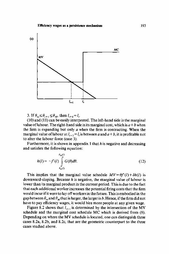
Efficiency wages as a persistence mechanism 193
(c)
MV
MC
(10) and (11) can be easily interpreted. The left-hand side is the marginalvalue of labour. The right-hand side is its marginal cost, which is a + b whenthe firm is expanding but only a when the firm is contracting. When themarginal value of labour at /,+ x = /, is between a and a + b, it is profitable notto alter the labour force (case 3).
Furthermore, it is shown in appendix 1 that h is negative and decreasingand satisfies the following equation:
G(9)d6. (12)
0m(D
This implies that the marginal value schedule MV=9f(l) + dh(l) isdownward-sloping. Because h is negative, the marginal value of labour islower than its marginal product in the current period. This is due to the factthat each additional worker increases the potential firing costs that the firmwould incur if it were to lay off workers in the future. This is embodied in thegap between 6m and 6M that is larger, the larger is b. Hence, if the firm did nothave to pay efficiency wages, it would hire more people at any given wage.
Figure 8.2 shows that lt+l is determined by the intersection of the MVschedule and the marginal cost schedule MC which is derived from (8).Depending on where the MV schedule is located, one can distinguish threecases 8.2a, 8.2b, and 8.2c, that are the geometric counterpart to the threecases studied above.

194 Gilles Saint-Paul
MV
MC
Figure 8.3 Effects of a small shock
Now suppose that figure 8.2a shows how the economy is 'normally'operating, say if 6 is equal to its expected value Ed. Suppose that there is asmall shock (i.e. 6t+l^ EO) that shifts the MV schedule. Then it is clear fromfigure 8.3 that if the shock is small enough, the size of the labour force isunchanged. Hence a first implication of the model is that it exhibits corridoreffects:
Small shocks have no effect on the level of employment
Consider now the impact of a large shock, for instance a contraction inperiod t+\. Then, as is shown in figure 8.4, the MV schedule shiftsdownwards, and this shift is large enough to imply a lower level ofemployment in period t + 1. but the relevant marginal cost schedule forperiod f + 2 will also shift since it has now a step at the new level ofemployment, //+1 < /, (see figure 8.4). Let M C be the new schedule.
Now assume that in period t + 2, 9 is back to its 'normal' value. Then thenew level of employment is given by the intersection of the MV scheduleand the M C schedule. It is clear from figure 8.4 that l(+2 = lt+,: the level ofunemployment does not return to its 'normal' value, and if 6 stays at itsnormal value, it will never do so. If the MV schedule were steeper than thatdrawn in figure 8.4, then employment would rise in period t + 2, but notenough to offset the drop in period t+\. Hence there is at least a part of thetemporary shock that persists for ever.
Hence another implication of the model is that:

Efficiency wages as a persistence mechanism
MV
195
MC
^+1 = h+2
Figure 8.4 Persistence of large shocks
Large transitory shocks have permanent effects on the level of employment
Notice, however, that this effect is smaller than the transitory effect thatwould be obtained if the firm was not paying efficiency wages (i.e. if the MCschedule was flat). Furthermore, the effect of the shock will persist onlyuntil a new shock changes the labour force.
Hence it is possible to obtain hysteresis in the context of an efficiencywage model. The pattern of employment obtained in our model differs fromthe Blanchard and Summers study in that the size of the shock matters:small shocks have no effect at all, whereas big shocks have permanenteffects. Another difference is that if the shock is really big, hysteresis will beonly partial, whereas in the Blanchard-Summers model, employmentfollows a random walk. Therefore, our model is more similar to the 'linearadjustment cost' or 'firing cost' view of hysteresis.
Joint behaviour of wages and employment in general equilibrium
The above results were derived under the assumption that the alternativewage, denoted by a, is a constant. Although this can hold in generalequilibrium for a given rule for the determination of unemploymentbenefits, this assumption prevents us from analysing the implications of thefact that the alternative wage is likely to rise in booms. What would beneeded, ideally, is to derive the joint behaviour of real wages and employ-
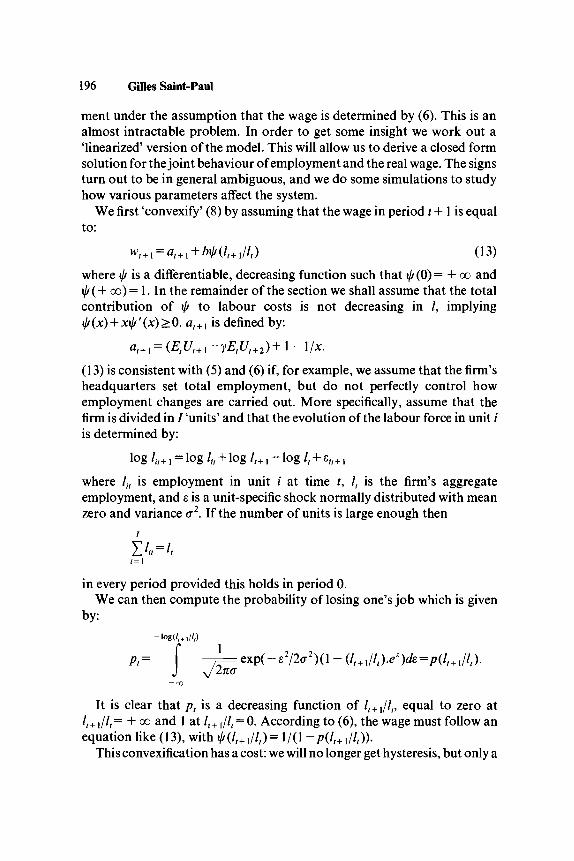
196 Gilles Saint-Paul
ment under the assumption that the wage is determined by (6). This is analmost intractable problem. In order to get some insight we work out a'linearized' version of the model. This will allow us to derive a closed formsolution for the joint behaviour of employment and the real wage. The signsturn out to be in general ambiguous, and we do some simulations to studyhow various parameters affect the system.
We first 'convexify' (8) by assuming that the wage in period t + 1 is equalto:
wt+l = at+l + biKlt+Jlt) (13)where ^ is a differentiate, decreasing function such that ^(0) = + oo andi/f(+oo)=l.In the remainder of the section we shall assume that the totalcontribution of \j/ to labour costs is not decreasing in /, implying
xil/'(x)>0. at+l is defined by:
at+l = (EtUt+l-yEtUt+2)+l-l/x.(13) is consistent with (5) and (6) if, for example, we assume that the firm'sheadquarters set total employment, but do not perfectly control howemployment changes are carried out. More specifically, assume that thefirm is divided in /'units' and that the evolution of the labour force in unit /is determined by:
log lit+! = log lit + log lt+ j - log /, + sit+!where lit is employment in unit / at time t, lt is the firm's aggregateemployment, and s is a unit-specific shock normally distributed with meanzero and variance a2. If the number of units is large enough then
1=1
in every period provided this holds in period 0.We can then compute the probability of losing one's job which is given
by:
-7 exp(-£2/2(72)(l - (lt+l/lt).eE)de=p(lt+{/lt).
It is clear that pt is a decreasing function of /,+1//,, equal to zero atlt+i/lt= + oo and 1 at lt+l/lt = 0. According to (6), the wage must follow anequation like (13), with <K/,+,//,)= 1/(1 -p(It+l/lt)).
This convexification has a cost: we will no longer get hysteresis, but only a

Efficiency wages as a persistence mechanism 197
positive serial correlation of employment in face of i.i.d. shocks. Thiscorrelation can however be made arbitrarily close to one by having a closeenough to zero.
The problem of the firm is then:
(pt t l t l t l t l t l t J t+ 8EtV(lt+l,Zt+l)
where Z is a set of exogenous variables which describe the state of theeconomy at date t, and hence determine the current and future behaviour ofthe variable at+l.
The first order condition can be written:
The envelope theorem implies:dV/dl=b(l?+l/lfW(lt+
Importing this into the first order condition one gets:
We now derive the behaviour of ar We first compute the expected utilityof an unemployed worker. Let wu be unemployment compensation,assumed constant, and n be the labour force. Then:• The number of people seeking work in period t + 1 is: n — lt+ptlt• The number of people being hired is: /,+ x — lt+ptlt• Therefore, the probability of getting a job in period t+ 1 is (ptlt + lt+x
-lt)l(n-lt+ptlt).Hence, one has:
(14)
Using (14) and (5) in the definition of a, one gets:
Hence the equations describing the behaviour of the system are:
liit)-bit+liw<J,M

198 Gilles Saint-Paul
1 *(*-/#(/,+,//,))•
along with (13), which describes the behaviour of the real wage.Our strategy is to loglinearize this system around a 'steady-state'.Let l=T(\+yt\ e=d{\+r]t\ at = a(\+zt\ W, = W(1+J , ) where y, z, s
and rj are small. The steady-state levels can be derived from the formulae:
Since we are interested in dynamics rather than steady-state levels, wewill not discuss them.
The dynamics of the system around (J, a) are described by the followingequations:
^/^+r" O7)
2 0 8 )where:
— 1) ———=ml/(\) — l J
and:
It can be shown (appendix 2) that (17) has one root between zero and one.If we assume that the other root is outside the unit circle, then (17) has aunique solution and employment follows an AR1 process:
where X is the stable root of c, + c2X + c3A2 = 0, and <P = c§k\cx. It is shown inappendix 2 that <P > 0. The 'sunspot' case where both roots are inside the

Efficiency wages as a persistence mechanism 199
unit circle and (17) has an infinity of solutions cannot be ruled out a priori.However, it never appears in the simulations that we present below.
Hence what efficiency wage implies here is a positively correlatedbehaviour of employment in face of i.i.d. shocks. We now turn to thebehaviour of the real wage. First, the alternative wage follows the process:
Hence the alternative wage is perfectly correlated with employment. Asshown by the simulations below, this correlation can be either positive ornegative. The real wage follows the process:
with:
Once again, the signs are ambiguous and the simulations will yield allkinds of results. The only thing that can be said is that if gx is positive, g0 ispositive. Hence one has three cases:• A positive response of the real wage to past employment and the
innovation in employment• A positive response to past employment and a negative response to the
innovation• A negative response to past employment and to the innovation.
The main conclusion is that the persistence mechanism due to the effortinducement problem does not necessarily imply a countercyclical real wage,as opposed to the partial equilibrium model studied in the previoussections. The downward pressure on wages due to a slump can well offsetthe upward pressure due to incentives while maintaining some persistence.However, as will appear from the simulations, the degree of persistenceconsistent with a procyclical behaviour of wages is limited.
Simulation resultsThe values of A,do + Adx,go and gx were computed for a 'plausible' set ofparameters implying an average unemployment level of 5 per cent. Theinterest rate was taken equal to 2 per cent for both firms and people,implying a typical period of about a quarter. The results are parametrizedaccording to three values:1. x, the probability of being caught shirking. The higher is x, the more
efficiency wage considerations are important.2. fi= —Tf"(T)lfQ), the curvature of the revenue function.

200 Gilles Saint-Paul
Table 8.1. Response of X,d$ + Xdx,g0,gx to \i
<T = 0 . 0 1 ; J C = 0 . 5
A*
0.10.20.51.02.0
X
0.890.880.870.850.81
0.850.700.27
-0.40-1.56
go
0.220.190.10
-0 .02-0.23
g\
-0.17-0.20-0.31-0.47-0.75
Table 8.2. Response ofX,d0 + ldx,g0,gx to x<7 = 0 .01; / / = 0.5
X
0.40.50.60.7
X
0.8710.8710.8680.863
1.130.270.100.001
go
0.120.100.100.004
g\
-0 .39-0.31-0.28-0.27
Table 8.3. Response ofX,d0 + Xdx,g0,gx to o
G
0.10.050.0250.010.005
X
0.530.650.760.870.92
do + Xd,
1.681.661.020.27
-0.16
go
0.480.480.310.100.001
g\
0.360.23
-0.06-0.31-0.42
3. <J, the 'diffusion parameter'.The results are reproduced in tables 8.1, 8.2 and 8.3 above. The main
findings are the following:• When x increases, X decreases: when monitoring is more efficient, it is less
necessary for the firm to promise higher wages in slumps, which lowers'pseudo-adjustment costs', thereby diminishing the amount of serialcorrelation.

Efficiency wages as a persistence mechanism 201
• When fi increases, k decreases: the more curved the revenue function, themore costly it is to deviate from the long-run optimal level of employ-ment. In addition to that, the simulations show that both the wage andthe alternative wage tend to be less procyclical when \i increases. Forexample, one gets the following results for a = 0.01 and x = 0.5. For lowvalues of /*, the alternative wage is positively correlated with employmentand the real wage positively correlated with lagged employment. Forhigh values of \i, these correlations are negative. In addition to that, theresponse of the wage to the innovation is always negative, all the more sosince \i is big. Hence, in order to get a high serial correlation and at thesame time a procyclical behaviour of the real wage, it is necessary toassume a low curvature of the firm's revenue function.
• The effect of a is also interesting. Not surprisingly, when a decreases, kincreases. This is because when a decreases, one gets closer to theprevious section's case where employment reallocation is fully concen-trated and hysteresis holds. However, when a decreases, the real wagebecomes less procyclical. Thus in our example, the real wage is positivelycorrelated with past employment and the innovation in employment for<r = 0.1 and cr = 0.05, but the latter correlation becomes negative for Gsmaller than 0.025 and the former becomes negative at a = 0.005. Hencethere is a trade-off between the amount of serial correlation one is able toget and the procyclicality of the real wage. Given that i.i.d. shocks at thefirm level were assumed, and that only a small amount of real wageprocyclicality is needed in order to match the data, we conclude thissection by saying that the model can generate an important amount ofserial correlation in employment while implying a procyclical real wage.Hence the previous section's results do not hinge on the convenientassumption that at is a constant. The fact that shrinking firms mustincrease compensation to induce effort from their workers does notnecessarily imply a countercyclical real wage at the aggregate level.
Conclusion
The main conclusion of this chapter is that a great deal can be learned fromextending the efficiency wage model in order to account for dynamicphenomena.
The main result is that the efficiency wage model can generate hysteresisin unemployment. Hence it can compete with the insider-outsider theory ofunemployment in order to explain this persistence. This is an importantresult in light of the fact that a lot of countries exhibit very persistentunemployment in spite of a very low rate of unionization (USA, France).

202 Gilles Saint-Paul
Furthermore the amount of persistence generated by insider models islikely to be small, both theoretically and empirically (see Layard, Nickell,and Jackman, 1991).
A natural extension of the model would be to include the calibrationexercise of the previous section in a full real business cycle model tocalibrate the joint behaviour of output, consumption, investment, unem-ployment and real wages.
Appendix 1: solution of the firm's optimization problem
The problem is:
V(lp9t+l) = max6t+ / ( / , + x)- {alt+1
Let us define EtV(lt+l90t+2) = H(lt+l) (9t+2 is independent of 0,+1);EtdV/dl(lt+u6t+2) = h(lt+l) = H'(lt+l).
It is clear that the solution must be of the following form:
mfoT0M<et+l9lt+l>lrIn order to solve this problem we must determine the critical values 6m
and 6M and the value of /,+ x when it differs from /,.(a) If / /+! < lt9 the first order condition (FOC) is:
6m must be the value of 6 such that this condition holds for lt+x = lt:
6m(lt)=(a-Sh(lt)W(lt).
In this case, the envelope theorem can give us the value of dV/dl(lp0t+l):
dV/dl=-b
(b)If/,+ 1>/,,theFOCis:
6M must be such that this condition is true for lt+x = lt:
The envelope theorem implies in this case:
dV/dl=0.
(c) Suppose now that 0t+l is between 6m and 9M. Then lt+l = lr As the

Efficiency wages as a persistence mechanism 203
firm's choice of /,+{is at the kink of the total cost function, we cannot applythe envelope theorem, but we can compute directly dV/dlt:
)
Since in this zone /,+ j = /, we have:
dlt+l/dl = \;dm<ix{ltjt+l}/dlt=\.
Hence:
+ 5h(lt)-(a + b)
which is between - b and 0 if 0r+1 is between 6m and 6M.Let us now compute the h function. Let G be the cumulative density
function of 6, g = G ' :
h(lt) = Et+ldV/dlt(lp6t+l).
The above calculations imply that:
oM
h(lt)= -bG{dm)+ ([0f(lt) + 5h(lt)-(a + b)]g(0)d0. (Al)
This implies that h{l) is always lower than 0 and greater than —bG(8 M).Furthermore, after integrating by parts, one gets:
oMd,)
h(lt)=-f(lt) f G(0)dO. (A2)
Appendix 2: properties of (21)
We have the following results:1. i/'/(l) + *A(l)>0. This is because we have assumed that the contribution
of \j/ to total labour costs was increasing in employment.2. i/Kl)> 1. This is because iA= 1/(1 -pt).3. d0 + dx > 0. To see this, compute it using the formulae of the text:

204 Gilles Saint-Paul
which is positive, since ^ ' < 0 , i^(l) + ^ ' ( l ) > 0 and \j/> 1.4. dx>0.5. 2\l/'(\) + il/"(l)>0. This comes from the second order conditions which
must imply that V be locally concave. One has d2V/dl2= —b(2ij/f(\)
6. cx > 0 derives from the previous result.7. cx + c2 + c3<0, since it is equal to STf (7)-(do + dx)<0.8. That cx + c2k + c3/l2 has one root between 0 and 1 is a corollary of (6) and
(7).9. That c0X/cx > 0 is straightforward.
NotesThis chapter was prepared for the University of Warwick Macroeconomic Work-shop (July 1993). I thank Olivier Blanchard, Athanasios Orphanides, Michael Pioreand Julio Rotemberg for helpful comments and suggestions1. The model has the feature that wages rise when employment goes down. One
might consider this feature as unattractive, since it is observed that the real wageis slightly procyclical. However, countercyclicality of the real wage is not impliedin a strict sense by our model. Rather, what is needed is just that totalcompensation be countercyclical. In particular, in Saint-Paul (1990), we extendthe model by allowing the firm to make severance payments, contingent on beingfired for a reason other than shirking. It is shown that this generates the samekinked labour cost function, but that the real wage can go either up or down inresponse to positive increases in employment. It will also be shown below thateven if all compensation is in the form of wages, procyclicality of the real wageholds in partial equilibrium, but not necessarily in general equilibrium.
2. More precisely the timing can be described as follows: each period t is divided inthree subperiods. In the first subperiod, the firm determines employment /, forperiod t. In the second subperiod, the value of 6t+l is known. In the thirdsubperiod, workers produce and are paid wages wt. What is crucial is that 9t+} isknown before period fs production is undertaken. Another assumption is thatno firing can occur in the second and third subperiod. This assumption impliesthat wt cannot be used to induce workers to work in period t, which simplifies theanalysis considerably. Although this structure might seem a little tricky, what isessential in the model is the interaction between the expected change inemployment and the incentives to shirk. The particular timing we use will allowus to translate the intuition into a very simple form for the labour cost function,but the results do not rest crucially on the particular set-up of the model.
3. The purpose of this chapter is not to analyse in detail the microfoundations of theefficiency wage model from the point of view of contract theory. For this we referthe reader to Carmichael (1985) and MacLeod and Malcomson (1993). Rather,we take the efficiency wage model as granted and derive its implication formacroeconomic dynamics.
4. An important issue is whether the firm will have an incentive to reveal its private

Efficiency wages as a persistence mechanism 205
information concerning tomorrow's value of 6. In Saint-Paul (1990), it is shownthat this is indeed the case.In Saint-Paul (1990), it is shown that under this cost structure the distribution offiring probabilities across workers has no effect on the total cost of labour. Theassumption of a uniform firing rule is therefore, innocuous.

9 Efficiency, enforceability andacyclical wages
Christian Schultz
Introduction
One of the puzzles of modern macroeconomics is the apparent lowvolatility of the real wage over the business cycle. Employment tends tovary too much compared with the real wage, at least if the data are to fitstandard macroeconomic models (see, for example, Blanchard and Fischer,1989, for a quick empirical overview). The purpose of this chapter is topresent a small model which can add to the understanding of why the realwage is so flat over the cycle.
We will study a simple example of a labour market where a firm employsa number of workers organized in a union. The union decides on the wage,the firm on the employment. The parties engage in a long-term relationship,and (as is well known) this gives them the opportunity to realize betteroutcomes than the one-shot non-cooperative equilibrium. The firm'srevenue is subject to stochastic shocks: in some periods the (linear) demandcurve is more favourable to the firm than in other periods. We focus on theefficient outcome sharing the surplus over the non-cooperative outcomeequally. Here the wage is lower than in the non-cooperative outcome, andin return the firm employs more workers than it would like to do at thiswage. When the parties' discount factor is sufficiently high, this outcomecan be implemented in each period in a subgame perfect equilibrium of theinfinitely repeated game. Although the firm in each period would like toemploy fewer workers at the efficient wage, it restrains from dismissingworkers, since the union will punish it for doing so in future periods bysetting higher wages.
However, since revenue is fluctuating there are some periods where it isparticularly tempting for the firm to deviate. In the chapter's model theseare the good periods. If the discount factor is only moderately high, thenthis temptation may become too big for the firm, and equilibria where thesurplus sharing efficient outcome is implemented in each period do notexist. The firm would deviate in the good periods. On the other hand there
206

Efficiency, enforceability and acyclical wages 207
are no enforcement problems in the bad periods. Evidently, it is best for theparties to implement efficient equilibria. Since the temptation to deviate forthe firm is increasing in the wage and it is only in the good periods that thistemptation is too high, the best the parties can coordinate on is anequilibrium where the wage is lower in the good periods than in the surplussharing efficient outcome, and where the wage in return is higher in the badperiods than in the surplus sharing efficient outcome. The enforcementproblems therefore induce a wage which is more flat over the cycle than isthe case for the surplus sharing efficient outcome. In fact, it turns out thatthe more flat is the wage, the smaller can be the discount factor without theenforcement problems becoming too serious. If the expected payoffs of theefficient outcome can be implemented, it can always be implemented by aconstant wage. Evidently, this wage also fluctuates less than the Stackelbergequilibrium wage.
Another possible explanation of the flat wage over the cycle is offered bythe theory of labour contracts (see, for example, the overview in Hart,1983). If workers are more risk-averse than firms, workers and firms haveincentives to construct labour contracts insuring the workers by having(relatively) flat wages over the cycle. In order not to replicate the results ofthis literature, we consider risk-neutral workers.
This chapter draws on Schultz (1993) where the same issues are con-sidered in a more general setting. Rotemberg and Saloner (1986) were thefirst to consider the best surplus sharing equilibrium in a model withfluctuating revenue and a moderate discount factor. They consider anoligopoly. Espinosa and Rhee (1989) consider a union and a firm in aninfinitely repeated game. They show that the efficient outcomes can besustained as subgame perfect equilibria for a sufficiently high discountfactor. Furthermore, for the case of fluctuating revenue and a moderatediscount factor they show that there are equilibria where inefficientoutcomes are implemented in each period. They do not consider whetherthere also are efficient equilibria in this case, and they do not try tocharacterize the behaviour of wages.
The organization of the chapter is as follows. The second section presentsthe model, and subgame perfect equilibria of the infinitely repeated gamefor high discount factors are studied in the third section. The fourth sectiondeals with subgame perfect equilibria of the infinitely repeated game whendiscount factors are moderate, and the fifth section concludes.
The model
We consider a firm and a union in a long-term relationship. Time evolvesfrom t = 0,..., oo. In each period, the firm produces output q by means of

208 Christian Schultz
labour input L. We assume that the firm has a constant returns to scaletechnology, so q = L. The firm faces a downward-sloping demand curve forits output, the inverse demand curve is p = a - q, where p is the price. Theintercept a is a stochastic variable which can take on two values <xg and oibwhere ag>(xb>0. The demand shock is independently and identicallydistributed over time, the probability of the good demand shock ccg is ij/,0 < \jj < 1. In each period both the firm and the union learn the shock beforeany actions are taken. There is symmetric information. This is an importantassumption for our results, but also a reasonable one. We conceive of thelength of time in which labour contracts are fixed as short relative to thelength of the business cycle. After having learned the shock, the union setsthe wage w for the period, and the firm then decides on the period'semployment L. Before the next period, the union sees how many wereemployed in the period.
The total revenue of the firm is T(L, a) = (a — L)L and the profit in aperiod is n (w,L, a) = (a — w — L)L. The firm seeks to maximize the dis-counted sum of expected profits, it has a discount factor <5, 0 < 5 < 1. Theunion's per period utility function is U(w, L) = wL. It seeks to maximize thediscounted sum of expected utilities, it has the same discount factor as thefirm.
Given the wage set by the union w, the profit maximizing employment forthe firm is Ld(w,<x) = . If the parties act non-cooperatively - as in theStackelberg equilibrium to the one shot game - the union takes this labourdemand function as given and chooses the wage which maximizes its utility,i.e. w which solves maxw wLd(w, a). The solution is ws(oc) = §. The resultingemployment in the Stackelberg equilibrium is Ld{ws{a),oi) = % The union'sutility then is Us(oc) = ws(oc)Ld(ws((x),(x) = i9 and the firm's profit is ns(u)EE (a - w*(a) - Ld(ws(a\ a))Ld(ws(a), a) = &
It is well known that the Stackelberg equilibrium is inefficient. The totalsurplus to be divided among the parties in a period isn (w, L, a) + U(w, L) = T(L, a). The maximal possible surplus is maxL T(L, a)= f > T + fg=£/*(a) + 7i5(a). The corresponding employment is L*(a) = f,higher than the employment of the Stackelberg equilibrium % That there is aunique efficient employment level is due to the special utility functionassigned to the union. While there is only one efficient employment level,there are many efficient wage rates, the union wishes high wages, the firmlow. In the sequel we will concentrate on the efficient outcome where theparties share the extra surplus over the Stackelberg equilibrium equally.This is obviously not the only conceivable outcome, but seems a natural oneto focus on. We will call it the efficient surplus sharing outcome. The resultswe will get will not change qualitatively, if we instead concentrate on someother outcome sharing the surplus in some (other) fixed proportion.

Efficiency, enforceability and acyclical wages 209
The total surplus to be divided is ^. In the Stackelberg equilibrium, theunion's utility is Us(oc) = y, and the firm's profit is ns(oc) = fg, therefore if theparties share the extra surplus the union's utility is £/*(a) = ^a2 , and thefirm's profit is 7t*(a) = ^a2. With the efficient employment L*(a) = §, thismeans that the wage of the efficient surplus sharing outcome is w*(a) = ^a.
The repeated game, high discount factors
In this section we will derive conditions under which the surplus sharingefficient outcome can be implemented in a subgame perfect equilibrium ofthe infinitely repeated game. The per period expected utility for the union insuch an equilibrium is EU* = il/U*((xg)+ (l — \l/)U*((xb), the expected perperiod profit for the firm is En* = il/n*((xg)+ (l — \l/)n*((xb). At time t, thehistory ht of the game consists of all previous shocks, wages and employ-ments. The union can condition its choice of wage in period t on this historyht and the periods shock a r When the firm chooses employment it cancondition on hp a,, and the wage set by the union wt. A strategy for the unionis a sequence of functions wt\ (hn a,) -• R, similarly a strategy for the firm is asequence of functions Lt\ (/*,,a,,w,)-> R.
We will now construct an equilibrium in which the players in the normalphase play the wages and employments belonging to the surplus sharingefficient outcomes. Since the firm has a short-sight incentive to deviate fromthe employment level L*(a), the equilibrium has to specify a punishmentfor the firm if it deviates. We will take the punishment to be infinite reversalto the one shot Stackelberg equilibrium. This is not the hardest conceivablepunishment. Since we are interested in conditions under which efficientoutcomes can be implemented, one could argue that we should use thehardest possible punishment for defections, cf. Abreu (1988). However, asargued by the literature on renegotiation - see, for example, Farrell andMaskin (1989) - one may wonder how reasonable mutually devastatingpunishment phases are. Such punishment phases will, although they arepart of a subgame perfect equilibrium, very likely be renegotiated by theplayers. Since this is not a chapter on the deep issues of renegotiationproofness we will simply content ourselves with looking at equilibria wherethe punishment consists of trust breaking down and players reverting tonon-cooperative play, i.e. reverting to infinite repetition of the Stackelbergequilibrium.
We claim that for a sufficiently high discount factor the followingprescribe the strategies of a subgame perfect equilibrium.• If / = 0 or only w*(a), L*(a) has been played so far, play w*(a), L*(a).• If the union in a period deviates to w ^ w* (a), the firm in that period plays
Ld(w,ot). In future periods, play w*(a), L*(a) unless somebody deviates.

210 Christian Schultz
• If the union plays w*(a) and the firm deviates from L*(a), or the unionplays w # w* (a) and the firm deviates from Ld(w, a), play ws(ot), Z/(a) inall future periods.With these strategies, the union can never gain from a deviation. If it
deviates, the firm immediately responds with employment on the labourdemand curve and this gives the union a utility which is less than or equal tothe Stackelberg equilibrium utility, which is less than the per period utilityin the equilibrium above. If the union deviates, the equilibrium prescribesthe best possible actions for the firm, so the firm will not deviate from these.Evidently, no one can gain by deviating in the punishment phase where theStackelberg equilibrium is played in each period.
Finally, consider the firm in the normal phase of the equilibrium. If itdeviates, it should deviate to the best possible employment Z/(w*(a),a),this gives the profit nd(a) = TC (w* (a), Ld(w* (a), a), a) = (^a)2. If the firm doesnot deviate in this period, it will receive profit 7r*(a) = ^a 2 in the period.Thus, the temptation to deviate is nd(ot) — n*((x)= (^a)2. Notice, that thistemptation depends on the state, and it is highest in the good state.
A deviation by the firm is punished by reversion to the Stackelbergequilibrium in all future periods. The expected loss of profits induced bythis is
\-8\Y32 v r / 3 2
Notice, that this punishment is independent of the state. Clearly, this isdue to the assumption that the shock is i.i.d. If the firm should not deviate ina state, the temptation to deviate should be less than the punishment, i.e. itis necessary that
§a2<14^(K2+O-</'K2)- 0)
The right-hand side is independent of the prevailing state, whereas theleft-hand side is higher in the good than in the low state. Furthermore, theright-hand side approaches infinity when 8 approaches one, it approaches 0as 8 approaches 0, and y ^ is increasing in 8. Therefore there are two critical<5s, 8b and 8g, where 0 < 8b < 8g < 1, such that, if 8b < 3, then the firm will notdeviate in the bad state, and ifdg<8, then the firm will not deviate also in thegood state. The higher is the difference between ag and ocb and the higher is i//,the higher is 8 and the lower is 8b.

Efficiency, enforceability and acyclical wages 211
The repeated game, moderate discount factors
Suppose now that the discount factor is not sufficiently high to prevent thefirm from deviating in the good state, i.e. assume that 3b < d < Sg. Then thesurplus sharing efficient outcome cannot be enforced in each period. Theproblem is that the wage in the good period is too high when the firm is toemploy the high number of workers L*(ctg). To see this, notice that at theefficient level of employment, the firm's temptation to deviate as a functionof the wage is
n(w,Ld(w,oc),cc)-n(w,L*(cc),(x)a — w\ a — w ( a\ a w2 ' '
This temptation is increasing in the wage. When bb < b < dg, the wage in thegood state is too high. On the other hand, the firm's gain from a deviation inthe bad state from L*(ab) (where the wage is w*(az,) = ^a^) is strictlysmaller than the punishment. Therefore the firm will not wish to deviate inthe bad state even though the wage is increased somewhat in this state. Thismeans that the enforcement problem can be relieved by lowering the wagein the good state, which makes the union worse off, and compensating theunion in the bad state by raising the wage there. This can be done withoutthe firm wishing to deviate in the bad state. Therefore, if the discount factoris below dg, but not too much below, there is an equilibrium where theplayers in this way achieve the same expected utility and profit as in the casewhere the surplus sharing efficient outcome is implemented in each period.Furthermore, this is the only way the players can achieve this outcome. Inthis case the wage is flatter over the cycle than the wage of the surplussharing efficient outcome itself.
We now show that if the difference between states is not too large there isa discount factor 5 where db<6<Sg, such that if S<S<Sg, then there is anequilibrium to the infinitely repeated game where the expected payoffs arethe same as if the surplus sharing efficient outcome is implemented in eachperiod and where the wage is the same in both states.
Theorem 1: There is a d where db<S<6g, such that if d<S<Sg,then the surplus sharing efficient outcome cannot be implemented in eachperiod in a subgame perfect equilibrium with Stackelberg punishment. Iffurthermore, \\j/0L2
g + (1 - \j/)ab(^ab -ocg)>0, then there is a subgame perfectequilibrium with Stackelberg punishment with expected average payoffsEU* and En*, where the wage is constant.

212 Christian Schultz
Proof: It follows from the previous section that the surplus sharingefficient outcome cannot be implemented in each period when 5 < dg.
Provided employment is efficient in each period, a constant wage givingthe union the same expected utility as if the surplus sharing efficientoutcome is implemented in each period fulfils
g ^ 0K2+ 0 -implying that
Then w*(ocg)>w>w*(a6), as ocg>ocb. Let the strategies be as in theequilibrium of the previous section with the only difference that the union inthe normal phase plays w rather than w*(a).
If the union deviates in a period, it can maximally get the Stackelbergutility in that period. If wL*(a)> Us(ct), then the union will never deviate.
(XThis is fulfilled in both states if w > ~. This condition can be rewritten
4\ ij/(Xg + (1 - \l/)oLb{^oib — ccg) > 0, which is the condition of the Theorem. (Thiscondition is fulfilled for ag and <xb sufficiently close or \jj sufficiently large.)
Clearly, just as in the previous section, the firm is interested in punishingthe union for a deviation.
If L*(a) is the employment and w the wage, the firm's expected profit isthe same as if the surplus sharing efficient outcome were implemented ineach period. Hence, since deviations are punished by Stackelberg reversion,the expected punishment is the same as in the previous section, i.e. equal to
6 ( a2 ab\^ i + 0 ~~ *A)^ )• Again this is increasing in 5. The temptation to32 32 J
deviate is given by (2). As w* (ccb) < w < w* (<xg), the temptation to deviate inthe present equilibrium is greater than it was in the equilibrium of theprevious section in the bad state but smaller than it was in the good state. Asthe punishment is increasing in the discount factor the theorem is proved.•
Notice that the condition on the as and i// is much stronger than needed inorder to ensure that the union will not deviate. It ensures that the union willnot even get a short-term gain from a deviation. If it was not fulfilled onecould still construct equilibria where the union would not deviate bymaking longer punishment phases for the union. As the above is just anexample, we did not find it worthwhile to introduce these extracomplications.

Efficiency, enforceability and acyclical wages 213
If the discount factor is exactly equal to d of the theorem, then the onlyequilibrium which implements expected payoffs equal to those of thesurplus sharing efficient outcomes is the one with the wage of the equili-brium. If the discount factor is higher, there are equilibria giving the sameexpected payoffs where the wage varies a little over states, but as long as thediscount factor is less than Sg, then the wage rate has to vary less than that ofthe surplus sharing efficient outcomes.
Concluding remarks
One may wonder how shocks to the slope of the demand function or to theproductivity of the firm affect the implementable wages over the cycle. InSchultz (1993) it is shown that for a class of examples with linear demandand constant returns to scale productivity shocks and shocks to the slope ofthe demand function give the same result as we got here. The temptation todeviate for the firm is greatest in the good state. If the discount factor ismoderate, then implementable outcomes will have a flatter wage over thecycle than the surplus sharing efficient outcome.
Another interesting question is how the results are affected if the shocksare not i.i.d., but follow a Markov process with persistence. In Schultz(1993) it is shown (in an example) that this does not change the qualitativenature of the results.
The Stackelberg equilibrium wage is ws(cc) = % it is higher in the goodthan in the bad state. It therefore follows directly that the wage implement-ing the surplus sharing efficient outcome for moderate discount factors isflatter than the Stackelberg equilibrium wage over the cycle.

10 Business fluctuations, worker moralhazard and optimal environmentalpolicy
Jon Strand
Introduction
The main purpose of this chapter is to study the relationship betweenenvironmental and employment variables in an economy subject to workermoral hazard, and the way this relationship is affected by environmentalpolicy. We consider two models. In model 1 (dealt with in the secondsection) firms face a stationary environment, while in model 2 (the thirdsection) the (exogenous world market) prices of firms' products fluctuaterandomly between a high and a low level, p0H and p0L. The main focus of thechapter is model 2, model 1 serving mainly as benchmark for the discussionof model 2.
In both models we assume that there is a worker moral hazard problem inproduction, in a way analogous to Shapiro and Stiglitz (1984), as workersmust have incentives to put up a given total effort level, enforced through awage exceeding the level clearing the labour market. This implies thatemployment in the economy in general is inefficiently low. In our set-uptotal effort has two components, namely output related effort, and effortthat serves to reduce pollution discharges from the firm (which are assumedto be perfectly observable by outsiders). The firm can decide how a totalworker effort x is to be composed of effort affecting output, y, and thataffecting environmental care, z. The firm is subject to a constant unitpollution tax r, set by the government. The firm's output may also besubsidized or taxed by the government, at a given constant rate.
For model 1 (dealt with on pp.217-24) we show that the level ofemployment (for the representative firm and for the economy as a whole) ingeneral is inefficiently low at a solution with no output subsidies. Assumingthat some unemployment always remains as part of an optimal solution,first best can be implemented by subsidizing output sufficiently, and letting texceed the (constant) marginal social damage cost from pollution, v. Withno output subsidies, the government may, as part of a constrained optimalsolution, choose to set t either higher or lower than v. t< v{t> v) when an
214

Business fluctuations and optimal environmental policy 215
increase in t also affects employment, N, negatively (positively). With noeffect of t on N, t = v. We also study balanced budget output subsidiesfinanced by pollution taxes. Under some assumptions these may implementa first best solution. When they do not, such policies are still more efficientthan using pollution taxes above. There is then always a tendency for t toexceed v, at the solution chosen by the government.
In model 2 (pp.224-30) we extend model 1 to a context of fluctuatingdemand, by assuming that firms' output prices in the world market jumpstochastically between a high and a low level, p0H and pOL, according to aPoisson process. In Strand (1991, 1992a) various aspects of such aneconomy have been explored. I have shown there that for small pricevariations, output and employment in each firm are fixed over time, whilefor larger price variations employment varies, but there is an extrainefficiency to employment in high-demand periods. In the context of thepresent model our conclusions now differ substantially, depending onwhether N(H) = N(L), or N(H)>N(L). When N(H) = N(L), a smallincrease in N(L) now automatically also raises N(H). This implies thatpolicies which increase N(L) now become more advantageous than in theone-state case. In particular, when only pollution taxes are used, t shouldnow exceed v by more for a given positive dN(L)/dtL, and both the L-periodemployment subsidy rate and pollution tax rate should be higher given abalanced government budget. In //periods employment subsidies are nowuseless (as long as N(H) remains unchanged), and the government prefersto set t=v. When we impose an intertemporal budget balance restriction,revenues from pollution taxes in both states should now be used tosubsidize L-period employment, i.e. the government budget will be under-balanced in L periods, and both tL and tH should exceed v.
When N(H)> N(L) at relevant solutions, the government's policy ineach individual state is now much as for model 1. The only difference isthat since the degree of employment distortion is greater in //periods thanin L periods, the employment subsidy rate should be higher in H periods,and the government budget underbalanced in H periods, given an inter-temporal budget balance restriction. Also here, tL and tH should bothexceed v.
The chapter provides a new approach to the analysis of employmentdetermination under fluctuating demand, by integrating work on environ-mental policy when workers' efforts are hard to enforce (Strand, 1992b,1992c) with work on business cycles under worker moral hazard (Strand,1991, 1992a). The basic idea is that firms' pollution to a significant degreedepends on the care taken by employees to avoid it, and that this care is partof an effort subject to enforcement by the firm. These higher demands onworkers' environmental care will affect firms' behaviour in other respects,

216 Jon Strand
through changes in the required non-shirking wage and/or other types ofeffort. Here we have simplified by assuming that total effort is constant, andthat required increases in environmental effort thus do not affect the wagebut only reduce productive effort requirements. This framework stillpermits us to derive several interesting conclusions, as referred to above.The most interesting of these can be restated briefly. First, when thegovernment can only use a proportional pollution tax, this tax will be sethigher or lower than marginal damage cost from pollution, depending onwhether the tax affects employment positively or negatively. Secondly, thegovernment revenue created by pollution taxes also provides room formore efficient policies by subsidizing employment, and gives the govern-ment incentives to increase the pollution tax more in excess of damagecosts. Thirdly, with demand fluctuations, we find for small variations inoutput prices that employment subsidies are more advantageous in low-demand periods, and that the pollution tax then should deviate more frommarginal damage cost, while for larger fluctuations the opposite may be thecase. For the conduct of environmental policy over the business cycle wethus reach no simple and clearcut conclusion: sometimes the environmentaltax should be raised going from a high- to a low-demand period, and atother times it should be lowered.
The amount of other literature directly related to the current chapter islimited. Besides the author's own studies already referred to (Strand 1991,1992a, 1992b, 1992c), we may mention a recent study by Gabel andSinclair-Desgagne (1993), which studies managerial incentives for environ-mental policy in a setting where managers may allocate effort amongdifferent tasks, among which is environmental care. That study uses a moretraditional principal-agent framework, whereby the managers' compensa-tion system trades off productive efficiency and insurance optimally forrisk-averse managers, but does not consider consequences for environmen-tal policy. There also exists an earlier literature discussing efficient environ-mental policy under different types of market imperfections, e.g. Buchanan(1969), Lee (1975), Sandmo (1975) and Barnett (1980).1 These studiesgenerally show that market imperfections create incentives for the govern-ment to set environmental taxes different from marginal damage cost. Wereproduce this basic result in a setting of worker moral hazard, but thescope of the present chapter is wider, compared both to these and the Gabeland Sinclair-Desgagne study, integrating environmental policy in a macro-economic and employment fluctuation framework. We may finally men-tion the recent work on constrained-efficient environmental policy, byBovenberg and van der Ploeg (1992, 1993) and Strand (1993a). Bovenbergand van der Ploeg show that employment may decline with higher

Business fluctuations and optimal environmental policy 217
government preferences for environmental care, even when the employ-ment tax is reduced (and the natural resource tax rate increased). This isgenerally in contrast to the main results from the present model. Strand(1993a) shows that in a distorted economy where individuals' behaviour isaffected by the pollution level, environmental taxes may be either above orbelow marginal damage cost, and that low taxes generally are conducive tohigh employment. Note however that none of these studies specifies anymicroeconomic model whereby labour market imperfections are explicitlyintroduced, in contrast to our model.
Model 1: the stationary solution
In this first model we study a stationary economy, with no changes overtime in the parameters facing the firms, nor in their behaviour. Assume thatthe number of firms in the economy is constant and normalized to one, andtheir output given by
Q=f(yN),f>0J"<0 (1)
where N is employment, N > N the labour force, and y is work effort put upby workers. Pollution from the firm is given by
h = h(N,z\ hN>0, hz<0, hNN>0, hzz>0, hNZ<0, (2)
where z measures workers' 'environmental effort' to avoid pollution.Increases in z reduce pollution, but at a decreasing rate while pollutionincreases with TV, possibly at an increasing rate. hNZ<0 implies thatincreases in z for all workers reduce pollution more, the more workers thereare.2
We assume that firms have limited capacity to monitor workers' efforts,and that both y and z must be enforced through an 'efficiency wage' in amanner analogous to that of Shapiro and Stiglitz (1984). Workers arecontrolled simultaneously for both regular work effort and environmentaleffort, at random intervals which are exponentially distributed with para-meter q. Define EV(N, N) as the worker's expected lifetime value from non-shirking with respect to both y and z, and EV(S,S) as the correspondingvalue when shirking with respect to both. We then have
) = w-y-z + b[EVu-EV(N,N)] (3)
) = w+(b + q)[EVu-EV(S9S)]. (4)
Here r is the common discount rate, b an exogenous turnover rate amongworkers, and EVU the value of being currently unemployed. (4) implies that

218 Jon Strand
the worker is always fired when caught shirking with respect to x =where x is total effort. It can then be shown that the relevant single non-shirking constraint for workers with respect to x is EV(N, N)>EV(S, S).3EVU is defined by
rEVu = s + c[EV(N,N)-EVu]9 (5)
given that all firms always enforce efforts and behave identically, where s isthe opportunity cost of labour (taken to be the value of non-marketactivities), and c the rate of jobfinding. We will assume that the firm candecide on y and z individually, at non-negative levels, but that their sumy + z = x is exogenous and constant. This implies that the total on-the-jobeffort of a worker who works efficiently is given, but that it can bedistributed between productive effort and environmental effort in any waypossible decided (and, we may assume, dictated) by the firm.
At an optimal solution for the firm, the worker non-shirking constraintEV(N, N) > EV{S, S) is assumed to be binding.4 This leads to the followingconstraint on the wage:
w*, (6)u ,
qor alternatively using (5), when all firms behave identically,
r+q+b+cw>s + — x. (6a)
Since EVU is exogenous to the individual firm, however, (6) is the relevantcondition on which to base the firm's decision on what levels of y and z toenforce. Here w* is defined as the non-shirking constrained wage. Note thatsince at equilibrium, flows into and out of unemployment must be equal,and that there is no shirking (assuming homogeneous labour),c - (N- N) = b • N, and thus b + c=[N/(N- Nb)]b = b/u9 where u is the rate ofunemployment. We here see that as w—•(), i.e. full employment, w* —• oo,implying that full employment in this sense can never be reached. We alsosee that for any (less than full) employment level, w* > s + y + z = wc, wherewc is the standard competitive wage in this case, for the given efforts y and z.This implies some inefficiency in the allocation of labour in the unregulatedmarket solution. We will, however, assume that/*(N) < s + y + z, given thaty and z are also socially optimal. As seen below, this assumption implies thepossibility for the government in principle to eliminate these labour marketinefficiencies, through appropriate taxes and subsidies.
The firm is assumed to maximize profits given by
n=pf(yN)-wN-th(N,z), (7)

Business fluctuations and optimal environmental policy 219
where p is the output price facing firms, and t is a unit tax on pollution,whose level is assumed perfectly observable by the government.5 From theassumptions made above, w > w* will be a strictly binding constraint onfirms in maximizing profits with respect to employment, N, and therequired levels of work and environmental effort, y and z. Above we haveseen that only the sum y + z = x is of importance for the determination of w.Assuming x constant implies dz= — dy.6 The first order conditions for thefirm with respect to N and z are then
dnf(N)w-thN(N,z)=o (8)
| j = -pNf(yN)-thz(N,z) = O. (9)
The effects of changes in/? and t on N and z are now found as follows:
^ ^ (10)
=^ [Phj+PNf"(NhN+yhz)-t(hNhzz-hzhNz)] (11)
(12)
\ [hf+f-iNh+h^iKhh^)]. (13)
HereD = (py2f ~ thNN)(pN2f"- thzz)- (pf +pyNf" + thNz)\ (14)
which is positive when the firm's second order conditions for maximumprofits are fulfilled. A necessary condition for an internal solution withrespect to both N and z is here that yhzz + NhNz > 0, and thus dN/dp > 0.7 Theother derivatives cannot be signed unambiguously from our assumptions.However, when hzhNN<hNhNz and NhN+yhz<0 (which both seem reason-able), dz/dt > 0. Intuitively, z increases in / since a higher environmental taxmakes it worthwhile for the firm to require more effort for pollutionavoidance, and relatively less for production activities. Reasonably also,dN/dt and dz/dp are both ambiguous. An increase in t thus lowers generalprofitability but increases the marginal productivity of TV since y generallydrops. This yields counteracting forces on the demand for TV. Similarly, anincrease in p increases N, but it is unclear how y, and thus z, are affected. Ifthe marginal efficiency in lowering pollution from increasing z is improved

220 Jon Strand
when L increases, z is likely to increase as well, while in other cases z coulddecrease. We will here make no specific assumptions about the signs oidNjdt and dz/dp.
Consider finally the effect of/? and t on z when N is fixed. We then find,differentiating (9):
* Nf «> 05)dp pN2f"-thzz
dz_ hz
Jt~pN2f'-th2>0. (16)
Here, consequently, environmental effort is always lowered when pincreases, since increasing p makes it more profitable to increase y. Asbefore, there is a positive effect of increasing t on z, which may be weaker orstronger than in the case of variable N (it is generally stronger here when Nthen decreases).
Define now the government's utility from firms' activity byG=pof(yN)-(s + y + z)N-vh(N,z). (17)
Here/?0 is the demand determined (e.g. world market) price of output, andthus p~po = p> a government subsidy rate on output, v is the (constant)marginal social damage cost of pollution. The government is consideredrisk-neutral and has no preferences for own revenues per se, ands + y + z = s + xis the social opportunity cost of labour given that not allworkers in the economy are employed.
Consider first the unconstrained optimal solution for the government,i.e. that chosen if the government could choose N and z directly. This isfound maximizing (17) with respect to TV and z (noting that dy = —dz),yielding
dGf(N)(+)vhN>o (18)
PoW(yN)vhz 0. (19)
Here (18) can be fulfilled with inequality if and only if N = N, andpoyf(yN)-vhN(N,z)>s + x (\Sa)
for the levels of y and z then found from (19). In such a case the first bestimplies that all workers are employed. The same holds when (18) is fulfilledwith equality for N= N. In other cases we have
N<N. (186)

Business fluctuations and optimal environmental policy 221
In such cases it is never socially optimal for all workers to be employed,since their marginal return would then be higher in other activities.
Consider now the possibility for the government to implement a first bestsolution, using the instruments p=p—p 0 and t, and assuming no govern-ment budget restrictions. Given that (18b) holds, (18)—(19) are identical to(8H9) given that
P-PJZ1 = A9 (20M21)Po v
where A is a positive constant, given by
(22)
(20)-(21) imply that implementation of a first best in this case requires apositive subsidy rate on output, and a pollution tax in excess of marginalsocial damage cost.8 Moreover, the relative subsidy rate on output is toequal the relative pollution tax rate in excess of marginal social damagecost, and both are to equal A. The constant A expresses the degree ofimperfection in the labour market due to the efficiency wage structure. Wesee that A may be sizeable in particular when q is relatively small and x largerelative to s. Note from above that when all firms behave identically, A maybe written as
- V *'q\ u
Thus when/ (N) > s + x, efficiency would require u = 0 and thus A = oo. Wefind the following expression for the firm's profits in an implemented firstbest solution:
nF= (1 + A)[pof(yN)- (s + x)N- vh(N,z)l (23)
which tends to infinity as u tends to zero.The implication of this is that whenever/f(J/V)>.s + >y + z, a first best is
generally unattainable, since an infinite amount of subsidy is necessary forits implementation. This is the same conclusion as was reached in a purework effort context (with no externalities) by Shapiro and Stiglitz (1984).Note here that when f(N)< s + x, a first best may be attainable in ourmodel, even in the absence of profit taxes or net subsidies of firms. Netsubsidies S are namely given by
S=Apof(yN)-(\+A)vh(N,z). (24)
Here S is always negative whenever A is sufficiently small, and positivewhen A is sufficiently large. The idea behind the implementation of an

222 Jon Strand
efficient solution when A is small is of course that the revenue from efficientpollution taxes gives room for a sufficient amount of output subsidy for thefirst best to be implemented.9
In the following we will generally assume that a first best is notimplementable in a budget balancing way (ruling out profit taxes con-sidered by Shapiro and Stiglitz), by assuming that A is above its criticalvalue yielding S=0 in (24). We will instead consider two different con-strained-efficient solutions, namely (a) the case with only pollution taxes,and (b) the case of budget balancing output subsidies and pollution taxes.
Environmental taxes onlyIn this case the government maximizes (17) with respect to t, taking intoconsideration that N and z are affected by t via (11) and (13). We find thefollowing expression:
YC [^ / (^ ) - (^^) -^ ] Yt- [PoNf(yN) + vhz] |=o.(25)
Here the first square bracket and dz/dt must both be positive. dN/dt isgenerally ambiguous from the arguments above. When dN/dt < 0 (> 0), theterm in front of dz/dt must be positive (negative), implying (using (9)) thatt< v(t> v) at the constrained-optimal solution for the government. Intuiti-vely, when dG/dz = O,t=v. When G is affected negatively through N (whichis the case when dN/dt <0), G must be affected positively through z. Thisimplies that z is below its optimal value, which is the case when t < v. Theopposite (t > v) holds when G is affected positively through N(dN/dt > 0). Ingeneral the level of t chosen by the government can then be either below orabove marginal damage cost.
Consider next the case where TV is unaffected by changes in t. In such acase the government always sets t = v, i.e. selects a 'first best' with respect toz alone.
Balanced budget changes in t and p
We now assume that the government may subsidize firms' output price p0 ata rate p=p—p0, but in a balanced budget way, i.e. such that total outputsubsidies cannot exceed total revenues from taxation of pollution. We willassume that A in (24) above exceeds the level yielding S= 0, i.e. the first bestis not implementable in this way for the government. This generally impliesthat the budget balance restriction will be binding for the government, andthe budget always balanced at equilibrium. This implies the condition

Business fluctuations and optimal environmental policy 223
(p-Po)f(yN) = t-h(N,z). (26)
When t changes, p thus changes according to
We thus have in this case (letting subscripts BB denote budget balance)
(8N\ =p-p,d_N dN\dt)BB t dp 8t
dz\ _pZp*dz todt)BB t dp df
The optimality condition for the government becomes identical to (25)except that dN/dt and dz/dt from (11) and (13) are replaced by (28)-(29).From the discussion above of the partial derivatives of TV and z we now findthat (dz/dt)BB is still most probably positive, and that (dN/dt)BB is now muchmore likely to be positive than in (11), in particular when (p—p o)/t is nottoo small. Since dGldN> 0 as before, (dz/dt)BB and (dN/dt)BB both positiveimplies dG/dz< 0. Comparing dG/dz to (9) now yields that t>v even whendG/dz = 0 (sincep>p0)- In this case we thus in most likelihood have t> v,using the results derived for case (a).
When a pollution tax is accompanied by a balanced budget outputsubsidy, it is thus more likely that the tax will be above marginal damagecost from pollution, and more so when it is above v in both cases.
Consider next a balanced budget increase in/? and t when JVis fixed. Notethat in this case there is nothing to gain in terms of efficiency by increasingboth/? and t, since as noted for case (a), a first best can be implemented for zusing t alone. We may still derive the optimal t in this budget balancing case.We find the following relationship between t and v:
i (30)PofiyL)
t must consequently also in this case exceed v. The reason for this is that pnow is raised above its socially efficient level. This must be counteracted bya similar increase in t, to make environmental effort and thus pollutionconstrained socially efficient.
Consider now the effects of a (permanent) increase in/?0. For given t, andp = 0, these effects on N and z are given by (10) and (12) with p— p 0. Ingeneral such an increase in/?0 will also induce a change in t. We will howeverargue that the effect through t is small compared to that throughp0 directly.

224 Jon Strand
A possible effect is likely to work via dG/dz in (25), where the term p0Nfincreases and makes dGjdz lower, thus increasing t. Such an effect will incase (b) be present both with a change only in t and with balanced budgetchanges in t and p.
We may also study the effect of a change in p0 when N is fixed. Then asbefore t=v independently of/?0, and the government policy is not affected.The change in z is then given by (15).
Model 2: environmental policy under productivity fluctuations
We now consider an extension of model 1 by letting the output price facingeach individual firm fluctuate between a high (H) and a low (L) level, pH andPL^(0,PH). TO keep matters simple we now focus on one particular firm,taking the rest of the economy as stationary and exogenous.10 Thetransitions between H and L, and L and H respectively, are governed byPoisson processes with constant transition rates equal to ax and a2. In thelong run the relative amounts of time spent in the H and L states are thena2/(ax + a2) and ax/(ax + a2), respectively.11 Using VN(i) and VL(i) to denotenon-shirking and shirking (with respect to both y and z) respectively, instates i=H, L, we may define
a2[VN(H)- VN(L)] (31)
rVs(L) = w(L) + (b + q){Vu- Vs(L)] + a2[VN(H)- VS(L)] (32)
ax(\-n)][Vu-VN(H)]+ axn[VN(L)-VN(H)}
+ axn[VN(L)-Vs(H)].
Here (as in Strand, 1991,1992a) n = N(L)/N(H) is the fraction of the firm'slabour force in H periods that is retained in L periods, where «e(0,l].Possible L-period layoffs are assumed to be made at random, and laid offworkers are not recalled nor given any economic compensation from thefirm.12 For non-shirking to be enforced the conditions VN(L)> VS(L) andVN(H)> VS(H) must be imposed. Assuming that these are both fulfilledwith equality at equilibrium, and taking F^as exogenous, the non-shirkingconstraints are (dropping subscripts)
V(j)-Vu = -x9i = H,L, (35)
while the solutions for w(L) and w(H) can be written as

Business fluctuations and optimal environmental policy 225
(36)q '1= ~ Lr + 1 + o + <*\(\ ~n)]x + s + rVu. (37)
Assume now that the firm maximizes current profits in any given statetaking its strategy in the opposite state as given. Current profits in L and Hperiods are given by
n (L) =pLf(N(L)) - w(L)N(L) - tLh(N(L), z(L))
„] N(L) (38)J " J
-tLh(N(L),z(L))) =pHf(N(H)) - w(H)N(H) - tHh(N(H), z(H))
(39)
+ ^xN{L)-tHh(N{H),z{H%
using that n = N(L)/N(H) in (39). We find the following first orderconditions with respect to N(i) and z(i):
=pLy(L)f(L)-w(L)-hLhN(L) = O (40)
= -pLN(L)f(L) - tLhz{L) = 0 (41)
wiD-^x-t^WKO (42)
dN(L)dn{L)dz(L)dn(H)
8j^=-pHN(H)f(H)-tHh2(H) = 0, (43)
where L and H now are used as shorthand notation for the levels of y, z andiVin the two states. In (42), inequality obtains only if N(H) = N(L). In caseswhere N(L)<N(H), w(H)>w(L) from (36)-(37). The reason is that L-period layoffs cause an additional exogenous risk for workers in H periodswhich must be compensated by a higher wage. Moreover, this effect ofN(L)on w(H) produces the extra term ax (y + z(H)) in (42), making the firm limit//-period employment and setting N(H) = N(L) on a strictly positive rangefor pH~pL. The solution thus implies that employment is rigid betweenperiods for such a range.13

226 Jon Strand
In studying properties of the solution (40)-(43), note that for given tL = tand/?L=p9 (40)-(41) for L periods are identical to (8)-(9) for the stationarymodel. The comparative statics with respect to changes inpL and tL are thenalso identical to those in model 1. As will be seen below, however, thegovernment's optimal solution with respect to tL (forpL=p) is generally notidentical to that in model 1.
Consider next H periods. As already noted, for small relative changes inp, N(H) = N(L), and only z may vary. Then the solution is again equivalentto that of model 1, given pH=p. In this solution we have t=v, whiledz(H)/dpH is given by (15). The conclusion then is that with only smallrelative price changes facing firms between the high- and low-demandperiods, employment will stay fixed, the environmental tax in the high-demand period will equal marginal damage cost, and environmental effortwill decrease and productive effort increase, in high-demand relative to low-demand periods.
In (42), the term (ajq)x creates the difference in firm behaviour from (40).Thus the higher ax is, i.e. the shorter H periods are on the average, thegreater is the range ofpH—pL over which N does not vary.
Assume now that pH—pL is sufficiently great for N(H)>N(L) at thesolution chosen by the firm. (42) is then fulfilled with equality. Since (ajq)xin (42) is a constant, this term does not affect any marginal conditions forthe firm. This implies that further increases in pH have the effects given by(40) and (42), for pH=p and a given t. Thus when t then is a constant,dN(H)/dpH> 0, while dz(H)/dpH is ambiguous as in (42).
We now study government behaviour when N(H) > N(L). Starting fromany given state, the government maximizes present discounted value of thesocial surplus created by the firm in question, with respect to currentparameters tt and pi9 i = H,L. Define these present discounted values byV(H) and V(L). We then have
- V(H)] (44)
- V(L)]9 (45)
where G(H) and G(L) are expressions equivalent to (17). These equationsyield
(46)
(47)
First best solutions are also here derived from maximizing G{H) and G(L)

Business fluctuations and optimal environmental policy 227
individually with respect to N(i) and z(z), i = H9 L, in a fashion equivalentto (18)—(19) (now assuming equality in (16) for relevant N(H) levels).Properties of such solutions are basically identical to those for model 1 in Lperiods, i.e. (18)—(19) then still apply, replacing p and p0 by pL and p0L(letting p0H and p0L denote the underlying exogenous unsubsidized marketprices). For //periods we find the related expressions:
P^™J»^ = AH, (48)-(49)POH
where
q s + x50
Thus in general the relative rates of employment subsidy and pollution taxshould both be greater in H periods than in L periods. This is due to thegreater amount of distortion from the first best at the market solution in Hperiods. The result is easily understood by considering a first best solutionimplemented in L periods, implying a relative output subsidy rate p* andpollution tax rate tL. If the difference between pH and pL is small,N(H) = N(L) given the same instrument values p£ and tL. This is clearly notfirst best, and a higher subsidy rate in H periods is required.
We will now study second best solutions for the government assumingeither that only pollution taxes are used, or that output may in addition besubsidized, but in a balanced budget way and insufficient for first bestimplementation.
Pollution taxes only
We may distinguish between two separate cases, namely(a) pOH-PoL 'small' and N(H) = N(L) at relevant market solutions; and(b) POH-POL 'large' and N(H)>N(L).We study these in turn.
N(H)=N(L)In this case we find for H periods:
dV(H)_ r + a2 dG(H) ax dG(L)dtH r(r + ax + a2) dtH rir + a^^) dtH
8G(H)dz(H)_ l }
a2) dz(H) dtH
noting that dG(L)/dtH=dN(H)/dtH = 0 in this case. This simply implies

228 Jon Strand
dG(H)/dz(H) = 0, i.e. -p0Hyf(H)-vh2(H) = 0, which in turn impliestH= v, using (43). Intuitively, f^here only affects z(H), and the governmentcan then set tH optimally, being concerned about z(H) only.14
For L periods we find
dtL ~r(r + al + a2)\_dN(H) dtL + dz(H) dtL
fdG(L) dN(L) dG(L) dz{L)~+ aL)\_dN(L) dtL
+ dz(L)' dtL
(52)= 0
when N(H) = N(L), dN(H)/dtL = dN(L)/dtL. To determine in which way tLmay deviate from v in this case, assume first the special (but relevant) case ofdN(L)/dtL = 0, implying dN(H)/dtL = dz(H)/8tL = 0 as well. We then end upwith dG(L)/dz(L) = 0 and thus tL= v as the government's optimal solution.Assume instead that dN(L)/dtL>0. Then dN(H)/dtL>0, and dG(H)/dtL>0 as well.15 In the opposite case of dN(L)/dtL<0, dN(H)/dtL anddG{H)jdtL are also negative, but the absolute value of the last expression isnow smaller.16
The conclusion is that when dN(L)/dtL>0, tL<v, while whendN(L)/dtL<0,tL> v. Qualitatively, this is as in the stationary model 1. Thedifference between tL and v is however greater here than in model 1, since theeffect on employment now also works via the opposite state H, in which thetax parameter tL is not directly applied. Note also that the difference tL - v islarger when it is negative than when it is positive (for given \dN(L)/dtL\),because of the effects via the term [dG(H)/dz(H)]-[dz(H)/dtLl
N(H)>N(L)In this case (42) holds with equality, and there is no direct
interlinkage between the strategies chosen by the firm in the two types ofperiods. This implies that the discussion from model 1 applies to this case,for Hand L periods separately. For Hperiods there is a slight difference dueto the inefficiency of unemployment being greater in this case and dG(H)/dN(H) generally greater at equilibrium.
Budget balance in each period
In the case of budget balance as an average over H and L periods, thefollowing budget condition must hold:
a2B(H) = axB{L\ (53)
where B(i) is the budget surplus in period / given (in a way analogous to(46)) by

Business fluctuations and optimal environmental policy 229
B(i) = tMi)-(P~Poi)f(i\ i = H,L. (54)
We will first consider only the case where budget balance is required for anygiven period, and then subsequently consider whether it is advantageousfor the government to make budget transfers between periods. Currentbudget balance implies, in a fashion similar to (28)-(29),
(dN(i)\ _p-PoidN(j) dN(i)
dz(J)\ =Pi-poi dz(i) + dz(i)*, ) B B U dPi dt, '
i=H,L. Also now we need to distinguish between the cases where N(H)= N(L\ and N(H) > N(L).
N(H)=N(L)Consider L-period strategies first. Assuming that dz(H)/dtL = 0,
we have, much as for P/=0 above, that (dN(H)/dtL)BB= (dN(L)/dtL)BB,which are both (almost certainly) positive. When compared both to model 1and to the case of p{—0 above, this makes it more advantageous to raise tL,since pL is then also raised, increasing both N(L) and N(H). Clearly, thisimplies that tL> v, and more so than for model 1. Environmental effort isthen above its first best level in L periods.
Consider next //-period strategies. Now dN(H)/dtH=09 and there isnothing to gain in terms of efficiency from increasing pH in a budgetbalanced way. Still, provided that balanced budget subsidies are used, tH isgiven by an expression analogous to (30).
N(H)>N(L)We now again have separation of the two types of periods, and tH
and tL are derived much as in model 1. The only difference is that also here(as with only environmental taxes above) the optimal tax and subsidy ratestend to be somewhat higher in H periods, due to the greater employmentdistortion in that state.
Intertemporal budget transfers
We may also now distinguish between the two cases considered above.
N(H)=N(L)In this case it is optimal to tax pollution while paying no employ-
ment subsidies in H periods, and to subsidize employment in L periods.Clearly, this implies that it is optimal to transfer funds from HtoL periods,

230 Jon Strand
making greater employment subsidies possible in the latter periods. Such astrategy will then raise employment in both states, for given implementedenvironmental efforts.
Moreover, the government's general need for funds to subsidize L-periodemployment makes it advantageous to set tH> v, and even possibly to tax//-period output as long as employment is not then affected negatively.
N(H)>N(L)In such cases the solution deviates little from the one-state model 1,
and there is little to gain from intertemporal transfers. However, since theemployment distortion generally is greater in H periods, a transfer from Lto H periods may now be necessary to implement the government'spreferred solution. In both types of periods tt> v, and possibly more so in Hperiods.
Conclusions and extensions
In this chapter we have studied aspects of efficient government policies todeal jointly with the problems of underemployment and pollution, in aneconomy where there are inefficiencies in the labour market due toproblems of disciplining workers' efforts, and where these efforts aredevoted both to the enhancement of firms' output and to the reduction oftheir pollution levels. A pollution tax will then have a joint effect on outputand pollution, and should generally be set below (above) marginal damagecost given that employment is affected positively (negatively) by the sametax. When the government revenue earned through the pollution tax is usedto subsidize employment, the preferred pollution tax rate is greater andmore likely to exceed marginal damage cost. We also have studiedproperties of the environmental tax under idiosyncratic fluctuations indemand, and found that the optimal pollution tax levels could be eitherhigher or lower in low demand, and the government budget underbalancedin low demand for small price fluctuations, but underbalanced in highdemand for large fluctuations.
The model studied is special since it assumes that the underlying labourmarket imperfection is of a quite specific nature, namely that of efficiencywages due to the possibility of workers shirking on the job. Still, we argue,the model gives important insights into the relationship between employ-ment and environmental variables, by building a micro-based, coherentmodel where the nature of the various inefficiencies and policy rules can bestudied in some detail. As such, our analysis should be just a start of a muchmore comprehensive effort to analyse such relationships. It can be arguedthat the employment and environmental policy areas are the two most

Business fluctuations and optimal environmental policy 231
important items on the public policy agenda, today and for the foreseeablefuture, for most rich as well as many poor countries. The interaction ofthese policies is no less important, but has so far been little studied.
A large number of extensions could be made to improve upon the currentanalysis and make it more general and topical. We will here briefly outline afew of these.
1. More general environmental problems could be addressed. For onething, environmental degradation due to the use of particular naturalresource inputs could be taken into account, as has already been attemptedin a related study by Bovenberg and van der Ploeg (1993). Among otherthings they address the so-called 'double dividend' hypothesis, wherebyhigher environmental taxes could at the same time help to increaseemployment, and answer this in the negative. Our analysis above indicatesthat the 'double dividend' hypothesis may hold when there are labourmarket imperfections, but this needs to be studied in a richer model wherenatural resource inputs are also included. Other extensions would be also tomodel the effects of firms' investments and of consumer behaviour onpollution and the policies to counteract it. Strand (1993a) attempts toincorporate the latter effect in an otherwise simpler model, and shows thatconstrained efficient environmental policy rules then generally becomemore complex. Moreover, general equilibrium effects, with full sets ofmarkets, should be considered.
2. Different and more general types of imperfections may be analysed.More general models of labour market moral hazard and adverse selection,or incorporating imperfections in capital markets affecting the investmentin both output- and pollution-related equipment, could be studied within aframework similar to that used here. Alternatively, the robustness andrelevance of our conclusions can be checked by constructing differentexamples of specific informational imperfections or practical limitations ongovernment policies. A relevant line of research, building, for example, onthe framework of Gabel and Sinclair-Desgagne, could be to study the firm'sincentives to take environmental care in a principal-agent relationshipwhere the incentives of managers would also be of importance, andincorporate this into a more complete markets framework.
3. The nature of the underlying fluctuations causing 'business cycles' inthe current model is quite special and could be generalized in future work.One obvious extension is to assume that the firm's output price changesaccording to a continuous distribution and not in a binary fashion. Such amodel is studied in a pure labour market framework by Strand (1993b). Ishow there that when firms' strategies otherwise are modelled as in thecurrent chapter, many of the same qualitative results are derived: inparticular, for a sufficiently dense price distribution employment will not

232 Jon Strand
vary with the price but be depressed to its lower-state level. With a moredispersed distribution of prices employment will vary but less than in astandard competitive economy. Quite likely this model could readily beadapted to incorporate environmental policy as here, with analogousresults. Another alternative would be to assume a random walk process forthe price, e.g., a continuous-time Brownian motion process. This has beenassumed in similar pure labour market contexts, e.g. by Bentolila andBertola (1990) and by Orphanides (1993). In such cases it is likely thatoptimal environmental and employment policy will not change much inresponse to price shocks, but this remains to be demonstrated. Finally,general equilibrium employment fluctuations (and not only partial equili-brium as here) should be studied. Strand (1992a) shows in a pure labourmarket context that with general equilibrium fluctuations the solution ingeneral becomes more complicated than here. Employment may thenfluctuate even less due to workers' alternatives being better in high-demandperiods. This probably makes it more advantageous to stimulate employ-ment in high-demand periods, relative to the analysis presented here. Thisand other extensions must, however, await future research.
NotesPaper presented at the University of Warwick Macroeconomics Workshop (July1993). I thank Jon Vislie and conference participants for helpful comments. Thisresearch is part of the project 'Environmental policy under asymmetric infor-mation', at the SNF Foundation for Research in Economics and Business Admi-nistration, Department of Economics, University of Oslo.
1. See Cropper and Oates (1992) for a survey of this literature.2. Perhaps more satisfactorily, pollution should be a function of the firm's output
and total environmental effort. We may then write
implying
Our assumptions are then made directly on /JN and hz.3. See Strand (1992b) for a discussion.4. A sufficient condition for this to hold is that/(0) = 0, i.e. when workers shirk and
put up no effort, output is zero. We will adopt this assumption in the following.5. Note that neither here nor in the following can the government do better by
using other environmental policies, e.g. transferable or non-transferable pollu-tion quotas. It is, however, true that in some cases non-linear pollution taxesmay be advantageous to use. These would, however, be equivalent to profit

Business fluctuations and optimal environmental policy 233
taxes, which we rule out. We may thus limit our attention to proportionalpollution taxes.
6. The justification for this assumption may be that working efficiently issomething well defined, implying a given total effort level, but that more or lessattention can be devoted to environmental care given an efficient total effort.
7. For example, in the case of h = h(yN), yhzz + NhNz = 0. In such a case we alwaysget a border solution with z = 0.
8. This is a basic result derived also for firms behaving monopolistically, andwhere there are no labour market imperfections; see Buchanan (1969) andCropper and Oates (1992).
9. It can, however, be argued that vh should be used by the government to clean updamages from pollution and/or compensate damaged parties. Then a netrevenue increase of vh would be required for the government to stay in balance,and firms would always be 'subsidized' according to (23).
10. Note that under such independent and firm-specific fluctuations and with acontinuum of firms, the entire economy will be stationary. In Strand (1991,1992a) I have, however, shown that the employment variations of a firm whoseproductivity fluctuates in such a way, adequately represents the employmentfluctuations at the macro level in the case where productivity shocks arecommon to firms, as long as such fluctuations are 'not too great'. The model canthus also give an approximate indication of how employment would fluctuate atthe macro level, given correlated shocks across firms.
11. These assumptions conform to those made in Strand (1991) for the case of noenvironmental effort.
12. For discussions of these assumptions and implications of alternatives, seeStrand (1991).
13. For details of such solutions with z = 0, see Strand (1991, 1992a).14. Here and in the discussions below we assume that the policies by government do
not lead to a change in the solution, from one where N(H) = N(L) to one whereN(H) > N(L). Such a change is more likely to be implemented by the govern-ment, the closer ph is to the level that yields equality in (42) in the absence oftaxation. Given such a switch, the analysis for the case o£N(H) > N(L) applieshere.
15. In fact the effect through z(H) is also positive, since dG(H)/dz(H) anddz(H)/dtL generally will have opposite signs.
16. This is because dG(H)/dz(H) and dz(H)/dtLnow are both positive, and thus theeffect on G(H) through z(H) positive.


Part IV
Financial market imperfections


11 The stock market and equilibriumrecessions
Jeff Frank
Introduction
A considerable number of recent studies have developed the multipleequilibrium approach to the understanding of Keynesian macroeconomics,as discussed in surveys by Dixon and Rankin (1991) and Silvestre (1993).Models in the literature show how imperfect competition and increasingreturns lead to multiple equilibria. Low level equilibria can be viewed asKeynesian in nature, particularly insofar as outcomes can be improved bycoordination or aggregate demand policies.
The purpose of this chapter is to explore the extent to which similarresults can be found in an economy with price-taking firms and decreasingreturns. The novelty in our analysis is the introduction of a stock market. Inan overlapping-generations economy with a stock market, there areinteresting multiple equilibria. A low output equilibrium, or 'equilibriumrecession', has the following characteristics. Real interest rates are high,capital investment is low and share values are low. These features areconsistent with stylized facts about economic recessions. This is an equili-brium since the low output and resulting low incomes lead to low savingsthat match the low investment.
An advantage of the current model is that it has the 'look and feel'associated with traditional macroeconomics as developed in IS-LM analy-sis. We develop the analysis with a flow market-clearing condition and withan asset market, portfolio-balance condition. The intersections of thesecurves determine the multiple equilibria.
The model
We examine a simple overlapping-generations stock market economy.1d'Aspremont et al. (1991a) and Pagano (1990) have explored multipleequilibria in imperfect competition overlapping generations frameworkswithout stock markets. Frank (1989) considers an overlapping-generations
237

238 Jeff Frank
stock market economy with imperfect competition. In that economy,multiple equilibria hold even in the presence of decreasing returns technolo-gies. The current model extends these results to an economy with price-taking firms.
The economy has a fixed number F of identical firms indexed by/ = l,...,Fthat exist indefinitely. All firms produce the same good whichcan either be consumed or used as capital. Physical capital is the sole factorused in producing output. In each period t, firm/hires capital Kft at therental Rt and uses the capital as the sole factor in producing its output Qft tobe sold at the price Pr
2 There are strictly decreasing returns to the firm'sscale of production: Qft = g(Kft) where g(-) is strictly concave.
Each period, the firm pays out its profits Ptg(Kft) - RtKft as dividends toits shareowners. Shares in the firm are traded on a stock market at a pricethat values the firm in total at the amount Vft. An individual buying y of firm/pays y Vft for the shares involved. Since there are no persistent effects to thechoice of capital, firms maximize profits by choosing Kft at each point intime t such that:
Ptg'(Kft) = Rr (1)
Households are part of an overlapping-generations structure and live fortwo periods; households are identical except for their age. //households areborn each period and each is indexed by its number h=l,...,H and its dateof birth t. When young, households receive an endowment in the amount e.This endowment is best viewed as labour services. The young sell thisendowment to the old of the previous generation at the price of labourservices Wv The young do not consume but instead 'invest' their incomeWte in physical capital and in buying shares of firms. When old, thehousehold receives rental on capital, dividends on shares, and the proceedsfrom selling its capital and shares.3 The household spends the receipts onthe produced good and on buying labour services from the young. Thehousehold gains utility from its consumption of the two goods (producedgoods bought from firms, and labour services bought from the young)following the quasi-concave, increasing utility function £/(•)•
The young face a portfolio choice between physical capital and shares inthe various firms. Depending upon the rates of return, they allocate theirendowment income Wte across the assets. In the absence of uncertainty, asin our model, we consider the perfect foresight rates of return. The rate ofreturn on physical capital bought in period / is:
Since each firm is identically placed in a given period, each chooses the same

The stock market and equilibrium recessions 239
capital and makes the same profits. The return on shares bought in period tis:
[Vt+l-Vt + Pt+lg(Kt+l)-Rt+lKt+l]/Vr
Households will only hold physical capital and shares in firms if each paysthe same return. This leads to the portfolio-balance condition for anyequilibrium:
Further, the total value of assets held by the h households must equal theirincome from selling labour services. The wealth-holding condition can bewritten:
(Vt + PtKt+l)F=WteH. (3)
The old face a choice between the consumption of the produced good andconsumption of labour services. Their income consists of dividends onshares, Pt+lg(Kt+l) — Rt+lKt+l, rental on capital, Rt+lKt+l, receipts fromthe sales of shares at the value Vt+l and the sale of capital Pt+lKt+l. Writethe total income at / + 1 of household h born at time t as Yhtt+l. Thehousehold spends this on the two goods. The demand for labour services attime f + 1 from this household can be written:
Lhj+\ = L(W(+l/Pt+l, Yht+l/Pt+l)
using the homogeneity of demand to write this in terms of the real wage andreal income. Walras' Law ensures that, if the labour services market and theasset markets clear, then the goods market must clear as well. The labourmarket clears if the total demand for labour services equals the supply fromthe next generation:
L(Wt+l/Pt+l,YhJ+l/Pt+l) = e. (4)
Equilibria in the economy must meet conditions (l)-(4) at each period intime t. We will consider only quasi-stationary equilibria. These are definedby a constant inflation rate n and therefore prices Pt = Px(\+ri){t~x\Vt= Vx{\ +nf~x\ W = Wx{\+n){t-x)<in(\R=Rx{\+n){t-x\ Further, capi-tal and output at each firm are constant at levels K* and g(K*). Then wehave the profit maximization and asset market-clearing conditions corres-ponding to (l)-(3):
g'(K*) = RJPx (5)
[g(K*) - (RJPX)K*]/(VX/PX) = RJPX (6)
VJPX + K* = (WJPx)(eH/F). (7)

240 Jeff Frank
The profit maximization condition (5) is that the marginal product ofcapital equals the real rental. Portfolio-balance (6) requires that the realrate of return on each asset is the same: the real profit level, divided by thereal price of shares, equals the real rental on capital. The wealth-holdingcondition (7) states that the real value of assets must equal the real incomeof the young, given that the young under our assumptions save all theirincome. Finally, we have the condition corresponding to (4):
L[WJPx,g(K*) + eWJPx] = e. (8)
The interesting feature of this condition is that, in a quasi-stationaryequilibrium, the real income of the old is just the real value of the producedgood plus the real income of the young. The reason for this is that the oldreceive dividends and rental income equal to the value of the producedgood; they then sell their shares and capital to the young for the totalincome of the young.
(5)-(8) define the quasi-stationary equilibria in the economy. In this non-monetary economy, it is not surprising that the price level and the rate ofinflation are indeterminate in equilibrium. Equilibria are defined by thecapital stock K*, the real rental on capital, the real wage and the real valueof shares. We will analyse the set of equilibria in the following section,showing by an example how multiple equilibria can arise.
An example
For further discussion, it is helpful to have a specific example. This requiresspecifying the production function g( •) and the demand for labour functionL ( ) , as well as numerical values for e,F,H. Consider the quadraticproduction function:
g(K) = aK-(b/2)K2
and the labour demand function (shown for household h at time i)\l/2]. (9)
This is the labour demand function for a household with an underlyingutility function in consumption of the two goods (the produced good andlabour services) U(cl,c2) = clc2/(cl + c2). Also adopt numerical values:e,H,F=l,a=\0, 6 = 2.
We proceed by solving (6)-(8), with the specific functional forms, for arelationship between the rental on capital (RJPX) and capital utilizationK*. As discussed earlier, the real income of a household in equilibriummeets YhJPt = g(K*) + eWJPx. Then from (8) and (9) we can solve for theequilibrium real wage:

The stock market and equilibrium recessions 241
Figure 11.1 Multiple equilibria in the asset market and the flow market
T = [g(K*)/e]2. (10)
Substituting (10) into (7), and then into (6), with the numerical valuese,H,F=\, leads to:
RJPx=\/[g(K*)]. (11)This condition represents asset market-clearing in our model. For eachlevel of capital and production, there is an interest rate that leads to a valueof shares equalling the labour services income of the young, net of their costof acquiring the physical capital. Incorporated within this relationship isthe determination of the real wage so that the demand for produced goodsand labour services equals their supplies, and the portfolio-balance con-dition that the return on physical capital and shares must be the same.
Under the quadratic production function, (11) takes on the form shownin figure 11.1 for the AM (asset market-clearing) curve. The remainingconsideration in determining equilibria in the model is the profit maximiza-

242 Jeff Frank
Table 11.1.
Equilibrium
HighLow
Equilibria with positive
K
4.980.01
R
Q
250.1
RJP,
0.049.98
K/Pr
6200.00002
tion condition (5). We view this as a flow market condition in that the FMcurve in figure 11.1 shows how the interest rate induces the firm to choosedifferent levels of capital and production. As seen in figure 11.1, there arethree intersections of the AM and FM curves, but only two of these withpositive returns to asset-holding.
For numerical calculations in our quadratic production function ex-ample, the AM curve takes on the form from (11):
RJPx=\/(\0K*-K*2) (12)
and the FM curve from (5):
RJPT=\0-2K*. (13)
Together, these lead to a cubic equation in K* determining the three rootsdiscussed above. Numerical calculations of the variables of interest for thetwo equilibria with positive Rx appear in table 11.1.
These equilibria meet reasonable stylized facts about macroeconomicfluctuations. The equilibrium recession is characterized by low output, highinterest rates and low share values.
The intuition behind our results is straightforward. A low interest rateinduces the firm to rent more capital and produce more output. But thehigher output also leads to greater savings, which allows for higher capital(and share values) to be consistent with a lower interest rate. The particularmechanism by which higher output leads to higher savings is peculiar to theoverlapping-generations structure. In that framework, the young save fromtheir wage income to provide pensions for their old age. Hence increasedlabour income raises the savings ratio, in contrast to the traditional stylizedfact that this type of redistribution lowers savings. In our example, higheroutput of the produced good leads to a sufficiently higher demand forlabour services that the savings ratio rises.
Given that we have examined an overlapping-generations economy witha number of stylized features, it may not be clear to what extent our resultsdepend upon the existence of a stock market. One way to investigate this isto consider what happens in the example as the parameter b in theproduction function approaches zero.4 When b = 0, there are constant

The stock market and equilibrium recessions 243
returns to scale in production and zero profits; as a result, shares in firmshave no value and there is effectively no stock market. To examine thebehaviour of the economy as b => 0 adopt the general quadratic productionfunction g(K) = aK— (b/2)K2, the labour demand function (9) and para-meters e, H, F= 1. Then as b => 0 the economy approaches the uniqueequilibrium defined by the equality of (5) and (11) with K*= I/a2. Thishighlights the role of the stock market in creating multiple equilibria.
Conclusions
Our analysis has developed multiple equilibria with price-taking firms anddecreasing returns to scale. We feel that this represents a significantstrengthening of the case for the coordination failure approach to under-standing macroeconomic fluctuations, since it generalizes the technologiesand market structures consistent with multiple equilibrium models.
The equilibria in the model meet sensible macroeconomic stylized facts inthat the low output equilibrium is also associated with high real interestrates and low share values. Another important feature of the framework isthat it displays a macroeconomic 'look and feel'. This is partially in that themodel emphasizes the role of financial markets in understanding macroeco-nomic fluctuations. More directly, the approach leads to asset and flowmarket-clearing conditions that mimic those of traditional IS-LM analysis.
Natural questions arise about the optimality and stability associatedwith the multiple equilibria. Scheinkman (1978) and Dechert and Yama-moto (1992) establish that equilibria in overlapping-generations stockmarket economies are efficient. This is an important difference between themultiple equilibria in our model and those of the imperfect competitionliterature. A second issue relating to policy implications involves thestability of equilibria. With only two equilibria, one will typically beunstable. These issues are discussed more fully in the related analysis inFrank (1994). In that model, it is seen that a shift to a high outputequilibrium benefits all future generations at the expense of the currentgeneration. The initial generation must increase its savings to allow for ahigher rate of capital accumulation, even though its income has not risen.The model also leads to an odd number of equilibria, so that there is both astable low and a stable high output equilibrium.
NotesI am greatly indebted to Heraklis Polemarchakis and numerous participants at theUniversity of Warwick Macroeconomics Workshop (July 1993). This chapter isproduced as part of a Centre for Economic Policy Research (CEPR) programme onThe UK Labour Market: Microeconomic Imperfections and Institutional Features,

244 Jeff Frank
supported by the UK Department of Employment (Research Grant No. 4RP-154-90). The views expressed in this chapter are not necessarily those of the CEPR or ofthe Department of Employment.1. Scheinkman (1978) and Dechert and Yamamoto (1992) develop the general
properties of overlapping-generations stock market economies.2. The results would be unaffected if the firms owned the capital.3. Note that the rental on capital, received by a generation born in period t, is Rt+]
on their capital Kt+l. This is an accounting convention, and the alternativeassumption, that they received R(, would make no difference to our analysis.
4. This point was suggested by Neil Rankin.

12 Asymmetric information, investmentfinance and real business cycles
Brian Hillier and Tim Worrall
It is not money that makes the world go round, but credit.Stiglitz (1988, p.320)
IntroductionThis chapter surveys the literature on the role of financial factors inexplaining economic fluctuations. We place special emphasis upon therecent literature on the implications for economic fluctuations of asymmet-ric information in the market for investment finance.1 The basic argumentof this literature is that, in the presence of informational asymmetries andagency costs, financial factors may affect real variables like investment andoutput. In dynamic models these real variables may also affect financialfactors and may generate persistent effects of shocks even in models whichwould not display persistence in the absence of the informationalasymmetry.
The plan of the chapter is as follows. The second section provides a briefdiscussion of the views of some earlier writers on the importance offinancial factors in the determination of economic activity. The thirdsection reviews the microeconomic arguments concerning informationalasymmetries and their implications for investment finance. The fourthsection shows one way in which these microfoundations have been used toprovide a real business cycle model based on informational asymmetriesand agency costs. We show that this model may yield multiple equilibriawith the possibility that the economy tends to oscillate around either a highoutput or a low output equilibrium. The fifth section reviews the literatureand the sixth section concludes.
BackgroundThe idea that the role of the financial system is important in explaining thecyclical behaviour of the economy has a long history. Fisher (1933) in his
245

246 Brian Hillier and Tim Worrall
theory of'debt-deflation' coupled the collapse of the financial system withthe collapse of real economic activity in the Great Depression. According toFisher the high level of borrowers' debt built up during the period ofprosperity preceding 1929 made the economy vulnerable to the ensuingdownturn which led to a wave of bankruptcies which, in turn, enhanced thedownturn. Furthermore, deflation reduced the net worth of borrowers andled them to cut back on their expenditures which, without any offsetting risein the expenditures of creditors, served to exacerbate the recession. Asimilar idea is suggested by Keynes who wrote that 'if the fall of wages andprices goes far, the embarrassment of those entrepreneurs who are heavilyindebted may soon reach the point of insolvency - with severely adverseeffects on investment' (1936, p.264). Keynes used this idea as one of hisarguments to explain why the market economy is not returned to fullemployment equilibrium by falling money wages and prices.2 In much ofthe General Theory, however, Keynes takes the failure of the pricemechanism as given and so works out the equilibrium of the economy forarbitrary values of money wages and prices. This latter exercise, although inmany ways less interesting than his arguments about the inefficacy of priceand wage flexibility for stabilizing the economy, was much easier toformalize and it provided the foundation stone for much of Keynesianeconomics and the misguided view that Keynes relied upon the liquiditytrap or wage rigidities to explain involuntary unemployment. The subse-quent debate between the Keynesians, monetarists and new classicaleconomists also tended to blur or ignore the fact that Keynes felt that themajor source of economic fluctuations was to be found in highly volatiledemand for investment and attention instead focused upon the monetarysector and developments of the theory of liquidity preference.3 Twoimportant reasons for the relative neglect of the investment sector were theforceful advocacy by Milton Friedman of the importance of the moneysupply, and the Modigliani-Miller theorem, which formally showed that ina perfect markets setting real investment decisions and the value of the firmdid not depend upon the method of finance.
Despite being out of the limelight, interest in the role of investment and inits mode of finance persisted in attracting the attention of macroeco-nomists. Notable among these were Gurley and Shaw (see, for example,1955), who noted the role of financial intermediation in the credit supplyprocess and called attention to the importance of 'financial capacity'.Financial capacity was an aggregate indicator of borrowers' ability tosupport debt without having to cut back current or future spending in orderto avoid default or rescheduling. The role of financial and balance sheetvariables on investment and output was thus emphasized in a mannersimilar to Fisher and Keynes.

Investment finance and real business cycles 247
Another important writer was Rosa who put forward the so-calledAvailability Doctrine that
in essence, it is not necessarily interest rates as a cost to the borrower, nor as aninducement to the saver, but rather interest rates as a reflection of underlyingchanges in credit availability, that have an important (though certainly not always adecisive) impact upon the generation of business cycles. (1951, p.276)Rosa's arguments focused attention on the issue of credit rationing andstimulated attempts to provide a sound theoretical explanation for thefailure of interest rates to rise to equate supply and demand in the marketfor loanable funds. These attempts in time led to the development of asubstantial literature on the role of asymmetric information in the creditmarket. This literature provides the microeconomic foundations for themodels of the business cycle which we review in this chapter. The followingsection looks at these microfoundations.
Asymmetric information and investment finance
Developments in the economics of information and incentives have beenapplied to both the equity and debt markets for investment finance andhave been used to explain the forms of financial contracts andintermediation.4
Consider the market for debt. There are three types of informationalasymmetry dealt with in the literature, either singly or in combination:(a) Borrowers may be indistinguishable ex ante. This may give rise to
adverse selection and Akerlof 's (1970) 'lemons' problem.(b) Banks may be unable to observe the use to which borrowers put their
funds. This may give rise to the problem of moral hazard with hiddenactions as in Arrow (1963, 1968).
(c) Banks may be unable to observe the returns to a project withoutincurring a cost as in Townsend's (1979) model of costly state verifica-tion. This may give rise to the problem of moral hazard with hiddeninformation since the borrower has an incentive to declare a projectreturn so low as to make him unable to repay his debt to the bank even ifthe return is in fact much greater than would be needed to do so. Inresponse to this problem, banks commit themselves to monitoring,either for sure or with some given probability, borrowers who default.5
Any of the above asymmetries of information may yield the result that anincrease, beyond a certain level, of the interest rate on loans may adverselyaffect the rate of return to banks. In the first case this happens by drivingborrowers with safer projects out of the market which, given the asymmetryin payoffs induced by the standard debt contract, is undesired by even risk-neutral banks. In the second case it happens by driving borrowers to choose

248 Brian Hillier and Tim Worrall
riskier projects, and in the third it happens by causing a rise in bankruptciesand an increase in monitoring costs. In each case the non-monotonicrelationship between the rate charged by banks and the return received bybanks may be used to explain the phenomenon of credit rationing: banksmay wish to hold the interest rate below the market clearing level sinceraising the rate would lower bank returns.
The early literature on asymmetric information and credit rationingplaced the emphasis on adverse selection and assumed that borrowers issuestandard debt contracts that pay lenders a fixed yield if the project return issufficiently high, or pay the entire project return if this is below the requiredfixed yield; see, for example, Jaffee and Russell (1976), Keeton (1979) andStiglitz and Weiss (1981). However, a problem with this literature is that theresults are sensitive to the nature of the distributions from which projectreturns are drawn; see, for example, de Meza and Webb (1987) who replacethe assumption used by Stiglitz and Weiss (1981) that the distributionsdiffer across projects in variances but not means by the assumption thatproject distributions differ in expected returns. Another problem is that theresults are sensitive to the nature of the financial contracts; see, for example,Bester (1985) who showed how the introduction of collateral requirementsmight be used by banks to induce borrowers to self-select themselves intodifferent categories and eliminate rationing, or de Meza and Webb (1987)who showed that the optimal mode of finance given the Stiglitz and Weiss(1981) framework was equity and not debt.
Even if equity is the optimal mode of finance, however, it is possible toshow that the agency problems which beset the debt market have theircounterparts in the market for equity; see, for example, Myers and Majluf(1984), Stiglitz and Weiss (1981), Greenwald, Stiglitz and Weiss (1984) andStiglitz (1988). Problems of a moral hazard or incentive type occur becausewhen a firm is equity-financed managers receive only a small fraction of anyextra profit so their incentive to expend effort on making profits isattenuated. Alternatively, since the owners or managers of firms haveprivate information about their firms' expected returns, it may be thosewith the lowest expected returns who are most willing to sell their shares,thus leading to adverse selection problems.
These informational asymmetries in either the credit or equity marketshow that investment may be constrained. The next section examines thedynamic macroeconomic implications of these constraints and attempts tofind some microeconomic foundations for the ideas of the earlier writerswhich were presented on pp.245-7. Given the variety of informationalasymmetries there are modelling choices to be made and we follow the routeof Bernanke and Gertler (1989). They introduce a costly state verification

Investment finance and real business cycles 249
problem where debt and retained earnings or net worth play importantroles. There are good reasons for adopting this approach.
First it is possible to show that in models with costly state verification theoptimal form of financial contract is a standard debt contract and that thiscontract is best intermediated by banks; see, for example, Diamond (1984),Gale and Hellwig (1985), Boyd and Prescott (1986) and Williamson (1986).The intuition for this result is simple. Given the informational asymmetrythe non-default payoff is a constant because no borrower would everchoose to pay to the lender more than the minimum amount necessary toprevent monitoring. The default payoff will equal the return to the project,since if it was less then it would be possible to raise it whilst lowering thenon-default payoff so that the borrower's expected repayment remains thesame; this would leave the borrower no worse off but yield a gain to thelender by reducing expected monitoring costs. Lenders monitor wheneverentrepreneurs claim to be unable to repay their loan since if they did not doso entrepreneurs would have an incentive to default and keep returns tothemselves even when projects were successful. Intermediation dominatesdirect lending since banks economize on monitoring costs; a bank monitorsa defaulting loan only once compared with each lender needing to monitorindividually under direct lending.
Secondly, debt and retained earnings are empirically by far the majorsources of investment funds, especially for small and medium sized firms(see Fazzari et al., 1988, Stiglitz, 1992 for some convincing evidence).According to Stiglitz this is partially a result of agency problems in theequity market. Thus he claims that
the cost of issuing equity is sufficiently great that most firms act as if they were equityrationed. When they are denied credit, they do not raise capital by issuing newequity, but rather constrain their capital expenditures to retained earnings. (Stiglitz,1988, p.313)
A real business cycle (RBC) model
Overlapping-generations model
In this section we present a slightly modified version of Bernanke andGertler (1989) who show how monitoring costs can produce low investmentequilibria and real business cycles. Their model introduces intragenera-tional heterogeneity and an asymmetry of information into the overlap-ping-generations model of Samuelson (1958). There are infinitely manyperiods but in any one period there are two equally sized cohorts, one in itsyouth and the other in its old age. Each cohort, distinguished by its date of

250 Brian Hillier and Tim Worrall
birth, consists of a continuum of risk-neutral agents called entrepreneurswho live two periods, their youth and old age, but consume only in their oldage.
There are two produced goods, an output or consumption good and acapital good. The capital good is produced using the output good as aninput and the output good is produced by a constant returns to scaletechnology using the capital good and labour as inputs. Capital goodsdepreciate completely after one period in use. There is also a constantreturns to scale storage technology to which everyone has access and whichtransforms one unit of the output good at the start of the period into r> 1units of the output good at the end of the period. We call r the gross rate ofinterest.
In their youth entrepreneurs are endowed with a single unit of labourwhich they supply inelastically to a competitive labour market which pays awage w (i.e. they receive w units of the output good) equal to the marginalproduct of labour at the end of the period. They save this w units of outputwhich then becomes their initial wealth or savings at the start of their oldage. Entrepreneurs must then decide whether to become capital goodsproducers. It is at this stage that heterogeneity is introduced: entrepreneurshave access to different capital good production technologies. In particulareach entrepreneur has access to an investment project which yields Z unitsof capital goods, where Z is a random variable, but requires a fixed input ofx units of the output good. The random variable Z is the same for eachentrepreneur independent of x, but x varies across entrepreneurs. Entrepre-neurs with low values of x are thus more likely to undertake investmentprojects.
There is also a simple asymmetry of information: when an entrepreneurundertakes an investment project only he can observe costlessly the actualnumber of units z of capital goods produced. Any other agent must pay amonitoring cost to observe the number of units of the capital goodproduced. It is assumed that monitoring of any project uses up m units ofthe capital good independent of z or x. We thus have a costly stateverification model of the Townsend (1979) type. As we have seen on p.249financial intermediaries or banks arise naturally in such an environment(see Diamond, 1984, Williamson, 1986) in order to economize on monitor-ing costs. These banks take in funds from entrepreneurs who decide not toinvest or have excess savings and they lend to others who wish to invest buthave insufficient funds. It is assumed that the banking sector is perfectlycompetitive so that each bank will make zero profits in equilibrium and thateach bank has a well diversified portfolio of loans. In addition it is assumedthat there are always sufficient funds in the economy to finance any level of

Investment finance and real business cycles 251
investment which the banks wish to fund, so the gross rate of interest paidon deposits at banks is r.
Capital goods produced but not used up in monitoring will be supplied toa perfectly competitive capital market at a relative price q in terms of theoutput good. Let k be the aggregate6 quantity of capital supplied. Inaggregate one unit of labour is supplied. Hence aggregate output is givenby/(&), where/( ) is the aggregate production function which is increasingand concave in k. As there are constant returns to scale in output goodproduction, the capital price equals the marginal revenue product ofcapital, f(k) and wages are equal to the marginal revenue product oflabour, f(k)—f{k)k. There are no profits in the output good sector.
The economy then proceeds as follows: at any date t the current old havesavings of st (the same for every member of the cohort). Old entrepreneursinvest or save and this determines the amount of capital goods produced,some of which may be used up in monitoring defaulting loans.7 The netamount of capital goods and the fixed amount of labour supplied by theyoung are then used as inputs to produce the output good. Because themarginal product of labour increases with capital, a larger net capital stockwill produce higher wages and hence higher savings for next period. The keyrole in Bernanke and Gertler (1989) is played by monitoring costs whichprovide a link between the entrepreneur's wealth and capital goodsproduction. No such link is present under perfect information.
First best case
As a benchmark we shall consider the first best case where there is perfectinformation, i.e. no private information, so that the outcome of theinvestment process is observable to any agent at no cost, m = 0. Assume thatthe random variable Z has a continuous, differentiate probability distribu-tion function G(z) = prob{Z<z} with support [zmin,zmax] and density func-tion g(z).8 Let ze = \zdG denote the expected value of Z. Then an individualentrepreneur, taking q as given and borrowing if necessary at the rate r, willundertake his investment project if ze>rx/q, i.e. if the expected returnexceeds the opportunity cost of investment in terms of capital goods. Writex(q) = qze/r, since ze and r are given parameters of the model but q is anendogenous variable. We shall assume that agents have perfect foresight sothe capital goods price q they expect is the equilibrium price. An entrepre-neur with x<x{q) will undertake his investment project but an entrepre-neur with x>x(q) will put any savings in the storage technology or ondeposit at a bank. Let H(x(q)) denote the proportion of entrepreneurs withx<x(q) where we assume xe [0,xmax]. We can treat H(x) as a distribution

252 Brian Hillier and Tim Worrall
function which we assume has a continuous density function h(x) withh(x) > 0 on (0, xmax). Hence aggregate investment in the economy is
x(q)
)= [xdH. (1)
We refer to i(q) as the perfect information investment schedule. Althoughthere is uncertainty about the production of capital goods at an individuallevel, since there is a continuum of entrepreneurs the law of large numberscan be invoked so that at an aggregate level capital goods production isnon-stochastic and given by
k(q) = zeH(x(q)) (2)where H(x(q)) is the proportion of entrepreneurs who undertake theirinvestment projects and ze is the average capital goods production of everyproject. We refer to k(q) as the perfect information supply of capital goodsschedule. The demand for capital goods schedule kd(q) =f ~l (q) is given byequating the capital goods price to the marginal product of capital. Asf" (k) < 0 and H(x) is increasing there is a unique equilibrium capital goodsprice satisfying zeH(x(q))=f~l(q) which we shall denote q*, with x*= x(q*), /* = i(q*) and k* = k(q*) denoting the first best levels. In order tomaintain the assumption that r is fixed it is necessary to assume that there isalways an excess supply of savings, i.e. st>i* for each time period t. Thedynamics in the perfect information case are trivial. In period 0 with savingss0, /* is invested producing a capital stock fc* which commands a price q*.The wages of the young are w* =/(&*) —f(k*)k*, the marginal product oflabour. This becomes the next period's wealth or savings, sx = w* so that /*is again invested, the capital stock is k* and output is f(k*), i.e. theequilibrium level of savings st = w* is attained after one period.
Optimum financial contractNow consider the situation with the asymmetry of information where theoutcome z is private information of the entrepreneur but can be observed byother agents at a monitoring cost of m > 0. First consider an entrepreneurentering his old age with savings s, who requires x units of the output goodto undertake his investment project and who expects a capital goods priceof q. Note that since the entrepreneur is small relative to the market, q willbe independent of his realized production level z. As in the perfectinformation case, we maintain the perfect foresight assumption that the qwhich each entrepreneur expects turns out to be the equilibrium q?

Investment finance and real business cycles 253
To determine whether an entrepreneur will undertake his investmentproject it is necessary to know on what terms he can borrow to finance hisproject. Suppose that the entrepreneur undertakes his project and lete<min(x,s) be his equity stake, i.e. how much he himself invests in theproject. If e < x then he must borrow the difference b = x — e from a bank.10
We assume that the loan contract with the bank can specify the equityparticipation e and that the creditor can costlessly access the entrepreneur'ssavings r (s — e)9 whether invested at another bank or invested in the storagetechnology, in the event of default on the loan. We can then appeal to theresults of Gale and Hell wig (1985) that any loan contract with equityparticipation e is weakly dominated by a loan contract with maximumequity participation e = s and that for the reasons described on p.249 theoptimum loan contract is a standard debt contract. A standard debtcontract has the following features: (1) there is a fixed repayment R, (2) thedebtor repays R if he is able, i.e. if z>R and (3) if he is unable to repay Rthen the debtor is in default and the creditor monitors at a cost m butrecovers the maximum amount of capital goods, i.e. z. Thus the optimumloan contract is entirely described by the repayment factor R.
Given the standard debt contract and with R specified, the borrower'sexpected repayment in terms of capital goods is
r T
p(R) = \zdG+ RdG.
Integrating both terms (the first term by parts) and rearranging givesR
rp(R) = R- G(z)dz. (3)
Likewise the creditor's expected return in terms of capital goods is
p(R)= !(z-m)dG+ [RdG=p(R)-mG(R). (4)
R
There are two points to notice here. First that p(R) is independent of x sincethe returns to investment are independent of x and second that thecreditor's expected return is equal to the borrower's expected repaymentless the expected monitoring cost, the latter being m times the probability ofdefault, G(R). The function p(R) is drawn in figure 12.1a. We shall assume

254 Brian Hillier and Tim Worrall
p, r(x - s)lq
(a)
Figure 12.1 Returns and repayments(a) Lender's return function (b) Repayment function

Investment finance and real business cycles 255
that it is a concave function, i.e. that mgr(R) + g(R)>09 and let^maxG[0>zmax] denote the repayment factor which maximizes p(R) and letPmax= PC max) denote the maximum value of the function. Intuitively, as Rincreases the creditor earns larger returns if the borrower does not default,but expected monitoring costs increase because there is a higher probabilityof default. Beyond Rmax the latter effect begins to dominate and thecreditor's return actually falls as R increases. Competition between banksmeans that R is never set above Rmax, otherwise another bank couldundercut and earn a higher return.
In a competitive equilibrium with free entry of banks and, hence, zeroprofits in the banking sector, the creditor's expected return on a loan of sizeb must equal the rate of return on a loan of size b available from the storagetechnology in terms of capital goods, i.e. r(x — s)/q. Hence
p(R)=p(R)-mG(R) = r(x-s)/q. (5)(5) determines R as a function of x for a given s and q, i.e. the terms on whichdifferent entrepreneurs can borrow, which we denote R(x;q,s) (entrepre-neurs differ only in x; each has the same s and expects the same q). Figure12.1b illustrates R(x;q,s) for a given q and s. For x<s there is no need forthe entrepreneur to borrow as he has sufficient funds himself, so R = 0. Fors<x<s + qzmjr then R = r(x — s)/q<zmin so there is no probability ofdefault, because the borrower can repay in full even in the worst possibleoutcome. The creditor therefore faces no risk at the individual level. Fors + qzmjr<x<s + qpmax/r the creditor does bear some default risk, G(R)>0, and R>zmin satisfies (5). For x>s + qpmajr there is no feasiblerepayment such that any lender does not prefer to place funds in the storagetechnology.
Within-period equilibriumHaving worked out the terms on which an entrepreneur can borrow it isnow possible to determine whether he would wish to borrow and thereforethe within-period equilibrium investment, capital goods production andprices. An individual entrepreneur will wish to invest if ze —p(R) > rs/q, i.e.if the expected return less the expected payment is no less than theopportunity cost of his funds. But from (5), p(R) = (r(x — s)/q) + rnG(R),where R = R(x;q, s). That is, the borrower's expected repayment must coverthe opportunity cost of the loan in terms of capital goods available from thestorage technology, plus the expected monitoring cost. Hence the entrepre-neur will wish to invest if
ze-mG(R(x;q,s))>rx/q. (6)

256 Brian Hillier and Tim Worrall
We graph both sides of (6) against x in figure 12.2 for given values of q and sand let x(q, s) denote the critical value of x beyond which investment is notundertaken. For x<s + qzmin/r, G(R(x;q,s)) = 0 so the left-hand side isconstant at ze, but for x>s + qzmin/r it declines until ze — mG(Rmax) atx = s + qpmajr, where we have drawn figure 12.2 assuming ze — mG(Rmax)>0. Figure 12.2a shows the case where savings, s are large enough or qsmall enough, i.e. s + qzmin/r>x(q) = qze/r or s>q(ze — zmin)/r9 so that thereis no need to monitor.11 In this case there is no risk of default for anyborrower and the asymmetry of information makes no difference. Projectsare undertaken if ze>rx/q, just as in the perfect information case.
Figures 12.2b and 12.2c illustrate cases which involve monitoring. Figure12.2b shows the case where x(q, s) < s + qpmajr. The marginal entrepreneur,for whom x = x(q, s), can obtain funds from a bank by offering the bank anexpected return of r(x — s)/q but will make an expected profit of zero fromhis project. The extra-marginal entrepreneur could also obtain funds, buthe would make negative expected profits and so would not undertake hisinvestment opportunity at the terms available in the market. In Figure12.2c, on the other hand, the marginal entrepreneur, for whom x = x(q,s)= s + qpmajr, will expect strictly positive profits but the extra-marginalentrepreneur is unable to obtain funds in the market because no lender willwish to lend to him. Since the extra-marginal entrepreneur would accept theloan contract of the marginal entrepreneur if offered to him, there is creditrationing.12 The important point for what follows, though, is not that creditmay be rationed but rather whether or not creditors expect to monitor, for ifthey do this will raise the cost of finance and reduce investment.
In the private information case the marginal investor has an investmentcost of x(q,s), which depends both on the expected price of capital goodsand, because of its effect on the probability of default, the savings level ofthe entrepreneur. In the perfect information case the marginal investor hasan investment cost x{q) — qze\r independent of entrepreneurial savings. Itfollows from what was said above that x(q,s)<x(q), with equality ifs > q (ze — zmin )/r (figure 12.2a) but with strict inequality for s < q (ze - zmin )/r(Figures 12.2b and 12.2c). For entrepreneurs with an investment cost of xsuch that s + qzmin/r <x<x(q, s), the existence of monitoring costs does notchange their investment decision but means that they must pay a higher costto obtain finance. For entrepreneurs with x(q,s)<x<x(q), monitoringcosts mean that they do not invest where in their absence they would havedone. Aggregate investment in the economy is then simply given by
x(q,s)
i(g,s)= [xdH<i{q) (7)

Investment finance and real business cycles 257
ze- mG(R), rxlq ze- mG{R), rxlq
(b)
*• x
z e - mG(R), rxlq
(c)
Figure 12.2 Within-period equilibrium(a) No monitoring (b) Monitoring (c) Monitoring and credit rationing
with strict inequality for s<q(ze-zmin)/r. This means that for a given qinvestment is either at or below the first best level.13
Figure 12.3 shows the response of x(q,s) to changes in q and s. It can beseen from figure 12.3, or implicitly differentiating (6), that x is increasing inq and is non-decreasing (increasing for s < q(ze- zmin)/r) in s. An increase inq has two effects (1) a direct effect on the value of the entrepreneur's returnand (2) an indirect effect through the reduction of monitoring costs: a rise inq reduces the repayment factor R for a given level of savings s<q{ze

258 Brian Hillier and Tim Worrall
(a)
ze-mG(R(x;q,sl))
\
x(q, sx) x(q, s2) x
(b)
ze-mG(R(x;ql,s))
/ rxlqx
ze-mG(R(x;q2,s))
x(qh s) x(q2, s) x
Figure 12.3 The response of x to changes in q and s(a) The effect of an increase in s:s2 > s}(b) The effect of an increase in q:q2 > qx
-zm i n)/r with the consequent reduction in the probability of default andhence monitoring costs. That is, an increase in q both increases theentrepreneur's gross expected return, qze/r, and reduces his expectedpayment, p (see (3)), since R is decreasing in q (see (5)). Hence marginalprojects become strictly profitable as q increases. An increase in s has onlythe indirect effect of reducing R and thus the probability of default and

Investment finance and real business cycles 259
expected monitoring costs; when s is larger, the loan size and repaymentrequired for any given x is smaller.
As in the perfect information case, because there is a continuum ofentrepreneurs, the law of large numbers can be invoked to show that eventhough capital goods production is random at the individual level, in theaggregate it is non-stochastic. Since all entrepreneurs with x<x{q,s)undertake their investment projects, total capital goods production iszeH(x{q,sj). Some of this capital goods production may, however, bedissipated in monitoring defaulting loans. Since default is a random eventat the individual level the cost of monitoring an individual project will be arandom variable,14 but again by the law of large numbers aggregatemonitoring costs will be non-stochastic and the quantity of capital goodssupplied as an input to the output market will be
x(q,s)
k{q,s) = zeH(x(q,s))-m f G{R(x;q,s)) dH<k{q) = zeH{x{q))o (8)
with equality for s>q(ze — zmin)/r (where there is no risk of default) andstrict inequality for s<q(ze — zmin)/r. We refer to k(q,s) as the privateinformation supply of capital goods schedule. For s<q(ze — zmin)/r thecapital goods supply to the market is less than in the perfect informationcase, k(q), because (1) fewer projects will be undertaken, x(q,s)<x(q), and(2) some proportion of the loans made to finance projects will be in defaultand so must be monitored, which dissipates some of the capital stock.Differentiation of (8) using (5) shows that k(q,s) is increasing in q and isnon-decreasing (increasing for s<q(ze-zmin)/r) in s. An increase in q hasthe above mentioned direct effect of increasing the supply of capital goodsbut the indirect effect works in two ways; it reduces the borrower'srepayment R, which encourages more entrepreneurs to undertake projectsand also decreases the probability of default and so the capital lost throughmonitoring. Increases in s have only these later indirect effects of decreasingcapital dissipated in monitoring costs and increasing the proportion ofprojects undertaken.
The capital market equilibrium is illustrated in figure 12.4. The demandschedule for capital, kd(q) =f~l (q), is drawn showing the equation of priceand marginal product of capital. Also drawn is the perfect informationsupply schedule for capital, k(q) = zeH(x(q)). The first best occurs at theequilibrium (q*,k*). Also drawn are the private information supplyschedules k(q, s) for three particular values of s. Higher values of s shift theschedule to the south-east. Let s* = q*(ze — zmin)/r be the smallest value of ssuch that the equilibrium outcome is (q*,k*). It can be seen from figure 12.4

260 Brian Hillier and Tim Worrall
q*
k{sx)k{s2)k*
Figure 12.4 Capital market equilibrium: s* > s2 > 5,
how the equilibrium quantity of capital goods supplied to the market andthe capital goods price depend upon the initial level of savings for s < s*. Wecan write these functions k = k(s) and q = q(s).
From figure 12.4 it is easy to see that in equilibrium q is non-increasing ins and k is non-decreasing in s. Intuitively higher savings reduce monitoringcosts so that there is a larger supply of capital for a given price q, i.e. anoutward shift of the supply schedule which depresses price and increasesquantity. Thus for s>s* the first best outcome is sustainable even withprivate information, but for s < s* there will be fewer capital goods used inoutput goods production and hence lower output. Once the capital goodsprice is determined for a given s, investment is determined by savings,i(s) = i(q(s),s). Similarly since the wage w equals the marginal product oflabour and this increases with the amount of capital used in production,wages are a non-decreasing function of savings since k(s) is non-decreasing,i.e. w(s)=f(k(s))—f(k(s))k(s) with w'(s)>0. In principle it is necessary tocheck that there is an excess of savings over investment, i.e. st> i(q(st),st) at

Investment finance and real business cycles 261
every time period in order to maintain the assumption that r is fixed, butfollowing Bernanke and Gertler we shall simply assume that parameters aresuch that it is always satisfied.
Deterministic dynamics
As we have said, even though capital goods production is random at theindividual level it is deterministic at an aggregate level. We therefore say theeconomy is deterministic. The only dynamics in the deterministic economyare provided by the savings variable; what entrepreneurs earn when youngbecomes their savings at the start of their old age (remember thatentrepreneurs do not consume until the end of their old age). But as we haveseen wages in the current period depend upon savings in the current period,so savings evolve according to a simple first order non-linear differenceequation given by st+x = w(st).
Figure 12.5 illustrates the possible steady-state equilibrium savings, se,where the function w(s) cuts the 45° line.15 Once equilibrium savings aredetermined, steady-state values of investment, capital goods production,output and prices are determined from the analysis of pp.255-61. There area number of cases to consider depending on the relative magnitudes of w*and s* and whether or not there is a unique equilibrium. First imagine thatsavings at time t are no less than s*. Then the equilibrium capital supply isk* with equilibrium wages w*=f(k*)-f(k*)k*9 so that next period'ssavings will be st+l = w*. Hence w(s) = w* for s>s*. Since s* = q*(ze
- zmin)/r it is possible that either w* > s* or w* <s*. In figure 12.5a w* > s*so that savings are sufficiently high in equilibrium to eliminate anypossibility of default. Hence there is a steady-state equilibrium withinvestment at the first best level and equilibrium savings se=w*. In figure12.5b w*<s* and there is a unique low investment equilibrium. Figures12.5c and 12.5d illustrate the possibility of multiple equilibria.16 Bothillustrate a stable high investment equilibrium and a low investmentequilibrium with an unstable equilibrium in the middle. The economy maytend to either stable equilibrium depending upon initial conditions. Infigure 12.5c the high investment equilibrium is below the first best level butin figure 12.5d the high investment equilibrium is equal to the first best level.
Stochastic dynamicsThe dynamics in the deterministic case are monotonic: savings, prices,output and capital stock simply increase or decrease toward their equili-brium values. If, however, there is a stochastic i.i.d. technological shock tooutput production, then it is possible to show that monitoring costs can

262 Brian Hillier and Tim Worrall
(a)
Figure 12.5 Dynamics(a) Unique full investment equilibrium(b) Unique underinvestment equilibrium(c) Multiple underinvestment equilibria(d) Multiple mixed equilibria
produce cycles or persistence and asymmetric responses. Suppose that thereis a random variable 0, with expected value of unity, which acts as amultiplicative shock to the output technology, so that output y = 6f(k). Wefollow Bernanke and Gertler and assume that debt contracts are madebefore 6 is known, but that labour and capital are hired after 0 is known.The capital goods price will then be a random variable and entrepreneursmust base their investment decisions upon their expectations of the price.Since they are risk-neutral their investment decisions are taken as if thecapital goods price were sure to be the expected price. The capital goodssupply curve will therefore be exactly as in the deterministic case, i.e. k{q\ s)where qe is the expected price. Given that the shock is unity on average, theexpected demand curve is just that in the deterministic case and it can be

Investment finance and real business cycles 263
seen from figure 12.4 that for a given level of savings, s, the equilibriumprice corresponding to the expected shock is q(s). Hence the rationalexpectations equilibrium supply of capital is k(s). Once 6 is known, priceswill adjust to clear the market, i.e. q(s,6) = df(k(s)) since the supply ofcapital goods is fixed in the short run, i.e. unresponsive to 0, and wages arew(s, 9) = 6(f(k(s)) -f(k(s))k(s)) = 6w(s).
Consider first the perfect information case in this stochastic environ-ment. In this case w(s,9) = 0w*, so a good shock produces higher outputand higher wages. Despite the fact that wages and thus savings arestochastic, investment next period is unaffected, since in the perfectinformation case investment depends only on the expected capital goodsprice, q*, and hence is independent of savings. Thus i.i.d. shocks toproductivity will cause i.i.d. shocks to prices and output but have no effectson investment or capital goods production.
Now consider the private information case. Since the first best equili-brium capital goods supply is k* at an expected price of q*9 it can be seenthat s*, the smallest savings such that the first best outcome is sustainable inthe private information case, is independent of 0. A positive shock, 9 > 1,then shifts the w(s) curve upward with no effect on s* and a negative shock,9< 1, shifts it downward. In order to examine the possible implication ofthis stochastic environment consider the following simple thought experi-ment. Suppose that there is a sequence of 9 = 1 shocks, so that the economysettles down at the steady-state equilibrium as if it were deterministic, butthen there is one positive shock, 9 > 1, before again the economy exper-iences a sequence of 9 = 1 shocks. Figure 12.6a illustrates the case wherethere is a unique low investment equilibrium. The economy begins in thelow investment equilibrium E when it is hit by a positive shock 9 > 1, whichshifts the curve upward for one period. Wages and output are higher thananticipated which feeds through to higher savings next period. By reducingtotal monitoring costs this allows more investment and capital goodsproduction next period, resulting in higher output and wages than normaleven though there is no new positive shock. There is persistence. In thewords of Bernanke and Gertler 'Strengthened borrower balance sheetsresulting from good times expand investment demand, which in turn tendsto amplify the upturn' (1989, p.27). There is also an obvious asymmetricresponse to shocks between an equilibrium with low investment and onewith the first best level of investment. If there were a unique equilibriumwhich sustained the first best level of investment with w* > s* then smallshocks would have no effect upon investment next period, whereas if thereis a unique low investment equilibrium even small positive or negativeshocks will cause persistent changes in future investment and capital goodsproduction. Furthermore, if there were a unique equilibrium which sus-

264 Brian Hillier and Tim Worrall
(a)
Figure 12.6 Effects of a temporary technological shock(a) Unique equilibrium with positive shock 6(b) Multiple equilibria with positive shock 6

Investment finance and real business cycles 265
tained the first best level of investment with w*>.s*, then whilst largenegative shocks would have an effect on investment, large positive shockswould have no such effects.
An even more interesting possibility is shown in figure 12.6b which showsmultiple equilibria; a high level locally stable equilibrium at E', an unstablemiddle equilibrium at G, and a locally stable low equilibrium at E. It is nowpossible that the economy displays temporal agglomeration - once at eitherthe high or low level equilibrium the economy tends to oscillate around itfor quite a while until a big shock pushes it past the middle equilibrium at Gand it then moves towards the other stable equilibrium. Suppose that theeconomy is at equilibrium E following a sequence of 6 = 1 shocks whenthere is a large positive shock which shifts the w(s) curve upward. Thisgenerates higher output and higher savings for next period and this maypush the economy beyond G and on toward the better equilibrium E' eventhough thereafter the economy experiences only shocks 0 = 1 . It is alsopossible that there may be asymmetries in the durations around high andlow level equilibria; if G is nearer to the low level stable equilibrium than thehigh level stable equilibrium, the economy would tend to be shocked awayfrom the low level equilibrium more easily than it would be shocked awayfrom the high level equilibrium and so would tend to be more often aroundthe high level equilibrium. Evidence for such asymmetric cyclical behaviourmay be found in Neftci (1984), Hamilton (1989) and Diebold and Rude-busch (1990).
Conclusions
Bernanke and Gertler (1989) have developed an equilibrium business cyclemodel in which financial intermediation plays a crucial role in explainingcyclical behaviour. The intermediation which takes place in the model fitswell with some of the features of real world financial markets. Intermediar-ies carry out the task of monitoring defaulting projects, they borrow fromlarge numbers of depositors and lend to large numbers of borrowers,writing debt contracts with borrowers and offering depositors financialassets which pay an expected return equal to the safe rate. The mainimplications of their model are:(a) Absent informational asymmetries, investment is unaffected by i.i.d.
shocks to productivity and output responses are non-cyclical.(b) With informational asymmetries i.i.d. shocks to productivity produce
cyclical responses in investment and output. The reason for thepersistence is that a good shock increases borrower net worth, reducingmonitoring costs and increasing investment and future net worth, andvice versa for a bad shock.
266 Brian Hillier and Tim Worrall
(c) The model may yield multiple equilibria with the possibility of temporalagglomeration or, in other words, the possibility that the economytends to oscillate around either a high output or a low outputequilibrium with a big shock needed to push it away from oneequilibrium to the other.
The next section reviews a number of similar models which can be foundin the literature.
Financial factors and business cycles
Apart from Bernanke and Gertler (1989) there are a number of othermodels of business fluctuations in which financial factors play a role.Bernanke and Gertler (1990) pursues the theme of the importance ofborrower net worth, but in a model where the asymmetric informationproblem is based not upon costly state verification but upon moral hazardwith hidden actions; entrepreneurs borrow in order to evaluate projects butlenders cannot observe whether they actually do evaluate (moral hazard),nor can they observe the information revealed by evaluation (which revealsthe success probability associated with a project to the evaluating entrepre-neur). Despite the differences, the critical role of net worth in easing agencyproblems remains essentially the same as in their 1989 study, although thelatter does not emphasize its role in propagating business cycles. In animportant development, Gertler (1992) returns to the problem of costlystate verification but extends the analysis to allow for multiperiod financialarrangements. This makes agency costs depend upon the present dis-counted value of future project earnings as well as upon the borrower'scurrent net worth. Thus a small change in macroeconomic conditions mayhave substantial effects upon expected future earnings and produce largeshort-run shifts in financial constraints.
Farmer (1984) and Williamson (1987) also embed a costly state verifica-tion problem in an overlapping-generations framework similar to Ber-nanke and Gertler (1989). In Williamson projects differ in terms of themonitoring costs in the case of default, rather than the cost of funding, andthere are some agents who have no investment projects of their own. As inBernanke and Gertler (1989), and for similar reasons, credit may berationed in equilibrium; although in Williamson the allocation of credit isbased upon the (observable) cost of monitoring if a project fails, with creditgoing to borrowers with the lower monitoring costs. Net worth, however,has no role to play since Williamson assumes that individuals with projectshave zero net worth. The type of shock considered by Williamson alsodiffers from the shocks considered on p.261. In Williamson there are shocksto the riskiness of investment projects; he assumes there are two possible

Investment finance and real business cycles 267
states of the world, where one differs from the other by applying a meanpreserving spread to the distribution of project returns. With risk-neutralagents such a shock would have no macroeconomic consequences in theabsence of information problems, but with costly state verification theriskier state increases agency problems and leads to less investment inprojects. Since there is a one-period lag between making an investment andthe resulting production of output, this has a negative effect on investmentthe following year too, producing cyclical dynamics or persistence as inthe model on pp.249-66. The difference is that Williamson's modelformalizes the idea that business confidence is important in explainingoutput fluctuations.
In Williamson (1987) an important role is played by the demand formoney. He assumes that the consumption good is perishable betweenperiods so that his lender class, who supply labour when young but notwhen old, must either invest in projects (via intermediaries) or hold moneyif they wish to consume when old, thus yielding a role for money (i.e. valued,unbacked government securities). His model yields a positive correlationbetween the price level and real output, and negative correlations betweenreal output and business failures and real output and risk premia. It predictsthat intermediary loans and a nominal monetary aggregate Granger causeoutput. The results concerning the price level and nominal monetaryaggregates cannot be derived from Bernanke and Gertler (1989) whichneglects monetary factors, but clearly the two models are complementsrather than substitutes.
Greenwood and Williamson (1989) develop a two-country version ofWilliamson's model which examines the role played by financial factors andexchange rate systems in the international transmission of business cycles.The model displays monetary non-neutrality and positive comovementsamong national outputs, inflation and interest rates. The correlationbetween output and prices depends upon the source of disturbances,monetary shocks yielding a positive correlation and technological shocks anegative one. Exchange rate regimes matter for the variance of output, butwhich yields the lower variance depends on the source of shocks, forexample a flexible exchange rate regime yields a lower output variance inresponse to foreign monetary shocks than either of the two fixed exchangerate regimes considered.
There are also a number of other studies in the literature which includeimportant roles for financial factors in the propagation of business cycles.One approach adopted by Kiyotaki and Moore (1993) is to provide adynamic model of the enforcement problems in the credit market con-sidered by Hart and Moore (1989).17 Although the model is rather differentfrom the models of asymmetric information discussed so far, the results are

268 Brian Hillier and Tim Worrall
similar. As borrowers may repudiate their debt, creditors protect them-selves by securitizing loans and never allowing the size of the debt to exceedthe value of the collateral. Investment, and therefore output, is determinedby collateral values. Investment and output in turn determine futurecollateral values and yield multiplier and cyclical effects.
Another approach is presented in an interesting series of studies byGreenwald and Stiglitz (1987,1988,1993) and Stiglitz (1992). They developa model which produces a role for net worth or retained earnings inpropagating cycles very much like that in Bernanke and Gertler (1989) butwithout any credit rationing or explicit modelling of informational asym-metries. Greenwald and Stiglitz rule out equity sales by using the type ofarguments discussed on p.248, and they assume a perfect credit market;agency costs and asymmetric information, therefore, are used to justifytheir model but have no formal role to play within it. The role for net worthor retained earnings is introduced by assuming that the managers of firmsare risk-averse. Risk-aversion is introduced either by placing a cost onbankruptcy in the utility function of managers or by making their utility aconcave function of profits. In either case this makes managers wary of debtfinancing, since this increases the probability of bankruptcy. Hencemanagers increase investment and output if net worth or retained earningsincrease, as this enables a substitution of retained earnings for debt.Increased investment and output in turn maintain relatively high retainedearnings so shocks have persistent effects in much the same way as inBernanke and Gertler (1989). Investment is also sensitive to the riskiness ofthe environment in a similar way to that discussed with respect toWilliamson (1987) above, but now directly due to risk-aversion rather thanagency costs.18
Yet another approach is taken by Blinder (1987) who, like Greenwaldand Stiglitz, assumes that there is no equity market but allows for creditrationing. Firms unable to obtain credit are unable to hire factors ofproduction and there is a failure of effective supply. Whilst the modelsBlinder uses are rather more ad hoc than those we have examined, he is ableto take advantage of their relative simplicity to integrate issues of aggregatesupply and aggregate demand. It would be interesting to do this in themodels with richer microfoundations which have so far tended to focusmore on the supply side; this is clearly an important task for future research.
ConclusionsWe have reviewed the recent literature which provides microeconomicfoundations for the long-established idea that financial factors are import-ant in explaining business cycles. Agency costs, enforcement problems or

Investment finance and real business cycles 269
risk-aversion have been shown to offer possible explanations of cycles. Inthis concluding section it is useful to compare these explanations withothers, briefly review the available evidence and offer a general evaluation.
It is possible to discern four major theories of business cycles (see Stiglitz,1992): the theory we have reviewed here based on asymmetries of infor-mation, the standard real business cycle (RBC) model (without informa-tional asymmetries), the new classical model of price forecast errors, andmodels of imperfect competition. The standard RBC model has been muchcriticized on the grounds that it relies too much on large technologicalshocks as the primary source of economic fluctuations (it is difficult to findnegative shocks to productivity of the size required to explain the GreatDepression), and too much on intertemporal substitution effects to explainfluctuations in employment (see Mankiw, 1989, p.79). Furthermore itmight be expected that changes in investment are dampened rather thanexacerbated as entrepreneurs take advantage of the reduced costs ofinvestment in recessions. The new classical model introduces the extraelement that agents may mistake general price level changes for relativeprice changes and respond accordingly, but this still fails to explain thecyclical volatility of investment. Similarly whilst the degree of competitionmight decrease in a downturn causing further reductions in output, sucheffects also have unrealistic implications, e.g. that profit margins arecountercyclical.
The view that financial factors are important in propagating businesscycles might be viewed as complementary to the above three approaches.But it also has some advantages. First, as we have seen, it is not necessarythat average productivity be affected since a small change in the perceivedriskiness of the economic environment can have significant effects viaagency costs (Williamson, 1987) or risk-averse behaviour (Greenwald andStiglitz, 1993). Second it has been suggested by Gertler (1992) that smalldisturbances can induce large output fluctuations when borrowers andlenders enter into long-term debt contracts. In that case net worth includesthe present discounted value of anticipated future project returns and, sincethis may be quite volatile, it is possible that small shocks produce largechanges in the cost of external finance.
We have so far concentrated upon theoretical issues. There is someempirical evidence which offers some support to the importance of financialfactors in explaining business fluctuations. Fazzari et al. (1988) examineevidence from the USA and conclude that financial constraints are import-ant for many firms and that their investment is positively related to retainedearnings or cash flow. An important aspect of their analysis is that theystudy investment behaviour in groups of firms with different financialcharacteristics and so offer a potential reconciliation of the mixed results of

270 Brian Hillier and Tim Worrall
earlier studies on financial factors in investment: financial factors may wellmatter more for some firms (new and small ones) than for others (estab-lished and large ones). Fazzari and Petersen (1993) present further evidenceof financial constraints on investment and consider the role of workingcapital. On a more macroeconomic level, Mishkin (1978) and Bernanke(1983) marshal evidence in support of the hypothesis that financial factorscontributed to the depth and persistence of the Great Depression in theUSA. More recently, Gertler and Gilchrist (1994) have found that, in theUSA, small firms account for a disproportionate share of the manufactur-ing decline following a tightening of monetary policy, and that balancesheets significantly influence small firm inventory demand.
We close with a few words on policy implications and directions forfuture research. The literature is, in fact, rather light on detailed derivationsof policy implications. Williamson, for example, concluded that 'thereappears . . . to be no obvious role for "stabilization policy'" (1987, p.1215).Stiglitz, on the other hand, concluded that 'an effective stabilization policyof the government should be directed at overcoming the limitations of [this]rationing' (1988, p.320) after discussing agency problems but withoutoffering a detailed analysis of such policy. Hillier and Worrall (1994) haveexamined a static version of Williamson's (1986) model and found the resultthat if rationing does occur then investment is likely to be excessive. Thereason is that the market outcome produces too much monitoring, so that acut in loan quantity increases welfare by cutting total monitoring costs.This result, whilst special to the model considered, illustrates that the policyimplications of such models may be quite different from the aggregatedemand management policies one might have expected from models withKeynesian features like interest rate rigidities. This is perhaps not sosurprising once one remembers that the models do not so much explainrigidities, but explain why prices which could move are sometimes heldconstant by rational optimizing agents. Nevertheless, there is a clear needfor further examination of policy, preferably within versions of the modelsextended to contain a government sector.
One way in which macroeconomic policy can have an effect in thesemodels has been examined by Farmer (1984, 1985), who showed that it ispossible for government debt and spending to generate real effects bychanging the real interest rate and affecting the level of investment. The realinterest rate is often fixed exogenously in the literature (it is given by thereturn on storage in the model on p.250, and by the imposed rate of timepreference in the Greenwald and Stiglitz models discussed above), and itmight be interesting to endogenize it to examine Farmer's arguments inother models. Another obvious implication of the models where retained

Investment finance and real business cycles 271
earnings matter for investment is that the average as well as marginal rate ofprofits tax matters for investment, a lower average tax rate raising retainedearnings and investment. This implication would appear to be testable.
We conclude that the literature on financial factors in macroeconomicmodels is interesting and promising. Further theoretical work is needed toexamine the policy implications of this sort of model and to introduce rolesfor other potentially important factors such as imperfect competition andmonetary surprises. Empirical work in this area is still relatively rare, andmore would be useful.
Notes
1. For a general survey of the role of asymmetric information in the market forcredit see Hillier and Ibrahimo (1993). An excellent earlier review with anemphasis upon the macroeconomic issues is Gertler (1988).
2. Recently Bohn and Gorton (1993) have presented a model of coordinationfailure which explains the use of non-indexed debt.
3. See the General Theory (1936, pp. 149-55, and 319-25) for support for the claimthat Keynes saw the volatility of investment to be the prime cause of outputfluctuations. Chapters 2, 3 and 4 of Hillier (1991) offer further discussion ofthese and related issues.
4. For surveys of the literature examining the implications of agency costs foroptimal contracts and the financial structure of the firm see Dowd (1993) andHarris and Raviv (1990).
5. The asymmetry of information identified in (a) is clearly ex ante because it existsbefore the debt contract is signed. That in (b) is ex post in the sense that thehidden action occurs after the contract is signed but ex ante in the sense that itarises before the project return is observed. That in (c) is clearly ex post since itarises after the contract and after the return is observed by the borrower.
6. All aggregate quantities are measured in per cohort terms.7. Initially it may seem puzzling that it is the old generation who may invest rather
than the young, but it is notationally convenient to keep investment and thereturns to investment in the same period. Thus the young enter the economywith no wealth and must work in the labour market to acquire wealth. As theyenter old age they make their investment choices and consume only at the end oftheir old age.
8. As stated above this section presents a slightly modified version of Bernankeand Gertler (1989). The main differences are: (1) they assume that Z is a discreterandom variable; (2) they allow for stochastic monitoring of returns in the caseof default whereas here we consider only deterministic monitoring: althoughthe macroeconomic properties of the model are unaffected by this change itallows us to interpret the optimal financial contract as a standard debt contract;(3) they introduce a class of lenders in their model, who do not have access to aproject of their own: this allows them to consider redistributions between
272 Brian Hillier and Tim Worrall
borrowers and lenders and show that such redistributions 'that may affectborrowers' balance sheets (as may occur in a debt-deflation) will have aggregatereal effects' (Bernanke and Gertler, 1989, p.28).
9. On p.261 an aggregate shock is introduced into the model so the perfectforesight assumption will then be replaced by a rational expectationsassumption.
10. We do not allow borrowers to borrow funds from several banks.11. If s is large or q is small the demand for funds will be low, either because
entrepreneurs can finance their own projects or because the expected return toinvestment in terms of output goods is low.
12. Credit is rationed, though, according to observable borrower characteristics,i.e. x, and is therefore quite different from the rationing of typical adverseselection models (see, for example, Stiglitz and Weiss, 1981).
13. We make no statements about whether it is at, below or above the second bestlevel.
14. If there is default then monitoring occurs for sure because we do not considerstochastic monitoring, but the event of default is a random variable.
15. The existence of an equilibrium is guaranteed since given our assumptions w(s)is continuous, w(0)>0 and the maximum of w(s) is w*.
16. Multiple equilibria appear to be a common feature of models of coordinationfailure in the New Macroeconomics literature. See, for example, Cooper andJohn (1988) and Bohn and Gorton (1993) as well as Frank (Chapter 11 in thisvolume).
17. Scheinkman and Weiss (1986) referred to such enforcement problems in theirstudy on borrowing constraints and aggregate activity, but did not presentdetailed micro foundations.
18. Stiglitz (1992) extends the analysis to argue that banks are a specialized kind offirm and that the principles which have been applied to other firms should alsobe applied to them. Thus, 'a reduction in the net worth of banks and an increasein the riskiness of their environment will lead them to contract their output, i.e.to make fewer loans' (Stiglitz, 1992, p.290).

PartV
Nominal rigidities and boundedrationality


13 Hedging, multiple equilibria andnominal contracts
Dawn Acemoglu
Introduction
Not all transactions take place in spot markets. Contracts are often writtento determine the terms of future trades. Understanding the nature ofcontracts is therefore an important step in the analysis of the allocation ofresources. A robust observation is that most contracts are not indexed tothe relevant price level despite the fact that prices at the time of transactionare uncertain and that the parties involved are risk-averse. This constitutesan important puzzle. A risk-averse agent would by definition benefit from areduction in risk. It would thus seem to be the case that two risk-averseagents would always prefer to turn a nominal contract they have signed intoa real one in order to reduce the risk they are bearing. The fact thatapparently risk-averse agents write nominal contracts when the aggregateprice level is unpredictable therefore constitutes an important puzzle.
A number of explanations have been offered to account for the presenceof nominal contracts. Gray (1976), Fischer (1977), Cooper (1988a) showhow in the presence of both supply and demand shocks the optimal degreeof indexation is less than full, and therefore how some degree of nominalrigidity can arise as an equilibrium phenomenon. However, this approachdoes not in itself explain why the majority of observed contracts are purelynominal (for instance Card, 1983, reports that about 50 per cent of US wagecontracts are not indexed at all, and the same applies with greater force toEuropean contracts). Here we can either appeal to bounded rationality orto costs of writing complicated contracts. In particular, an argumentsimilar to that of Akerlof and Yellen (1985a) and Mankiw (1985) can besuggested in this context (for example, Ball, 1988); costs of not choosing theright degree of indexation to prices may be of second order to individuals,while being first order to society. However, this argument is not verycompelling. Many contracts involve transactions for very substantialamounts between risk-averse parties and costs of non-optimal contractsmay be very large. Also in labour contracts signed between firms andunions, the cost of devising an optimal contract (especially if this contract
275

276 Daron Acemoglu
requires full indexation) that will cover a large number of workers is likelyto be small relative to the benefit. A different line of attack is to ask whetheran equilibrium with nominal contracts can be a 'self-fulfilling prophecy'.This intuition first suggested by Fisher has been developed by Cooper(1990). In Cooper's model, risk-neutral firms write commodity and labourcontracts with risk-averse workers/consumers. If all other firms are offeringreal contracts, it would be cheaper for each firm to offer a real contract butin contrast, if all other firms are expected to offer nominal contracts, thebest thing that the firm in question can do is to offer a nominal contract.
This can be thought of as part of a more general phenomenon we refer toas 'hedging via contracts'. When outside insurance opportunities arelimited, contracts written for transaction purposes will in general play tworoles; allocation of resources and allocation of risks. Suppose next period'sprices are random; a risk-averse agent would prefer to pay $50 and receive$50 in current prices simultaneously rather than receive $50 in currentprices and pay $50 in fixed prices. This is because in the second situation heis subject to the risk created by price uncertainty. By making both hisreceipts and payments in current prices (or fixed prices) he avoids this risk.Thus the agent may well prefer a nominal contract and the statement westarted with, that two risk-averse agents would always benefit from turninga nominal contract into a real one, is not true. This intuition suggests thatthe degree of indexation in contracts can in general be used to provideinsurance against risks associated with variations in the price level (i.e.'hedging').
We will first construct a simple model that exhibits these features and, asCooper's economy (1990), has multiple equilibria. As our economy issimpler than Cooper's, the basic mechanism will be clearer and we will beable to locate all the equilibria. Also as in Cooper's example, all theseequilibria will be efficient because they offer 'perfect hedging' to traders.However, more importantly we will show that when 'perfect hedging'through nominal contracts is not possible, all these equilibria disappear andwe end up with a unique equilibrium without any nominal rigidity. It thusappears that nominal contracting equilibrium is not a generic phenomenon.Nevertheless, we also show that when other imperfections are present, thisneed not be so. This result is in a similar spirit to Ball and Romer (1991),who show that real rigidities increase the impact of small nominal rigidities.However, the imperfections we consider are not real wage rigidities, butlimited insurance possibilities for agents and restrictions on the complexityof contracts that can be written. If there exist non-diversified risksassociated with changes in prices, the equilibrium contracts will no longerbe fully indexed. In particular, we show that in a dynamic overlapping-generations model where agents have limited access to financial instru-

Hedging, multiple equilibria and nominal contracts 277
ments so that they cannot insure against relative price changes, a nominalcontracting equilibrium may emerge, while a real contracting one fails toexist. Alternatively, when we restrict the complexity of contracts that can bewritten, we see that as well as the Pareto efficient real contracting equili-brium, an inefficient nominal contracting equilibrium becomes possible.We also obtain a number of interesting results; as in Ball (1988), writing anominal contract creates a negative externality but through a completelydifferent mechanism, and as in Mankiw (1985), small menu costs may havelarge impacts but again via a different channel. Underlying all these effectsis the desire of risk-averse agents to hedge. The more risk-averse are theseagents, the stronger is this mechanism. This can be contrasted to the Ball-Mankiw mechanism which gets weaker as the agents become more risk-averse, since increased risk-aversion raises the costs of non-indexation.
The plan of the chapter is as follows. The next section shows how amultiplicity of equilibria arises when agents trade with more than one party,but it is also shown that this multiplicity is not a generic feature. Thefollowing section analyses a dynamic economy with financial imperfectionsand demonstrates how a nominal contracting equilibrium may naturallyarise. The fourth section shows how a restriction on the complexity ofcontracts can lead to the presence of Pareto ranked equilibria. The chapterconcludes with a brief discussion in the fifth section.
A model with perfect hedging and multiple contracting equilibria
Consider an economy consisting of N agents denoted by /= 1,...,7V. Att= 1, if he buys one unit of good /— 1 as input from agent /—I, agent / canproduce one unit of consumption good and one unit of good i. Agent 1 buyshis input from agent N. Good / has no other alternative use and theconsumption good is sold in a competitive market. This situation can berepresented as the circle shown in figure 13.1. The single arrows show theflow of inputs and the double arrows show the supply of the consumptiongood.
We assume that agents can write contracts at time t = 0 to determine howthey will trade at t = 1. However, the general price level of this economy, /?,at which they will also sell the consumption good to the market, is uncertainwith a known distribution at t = 0, say because the nominal money supply isstochastic. Therefore, at t = 0 expected utility calculations are possible andwe ask what the equilibrium level of indexation will be in the contracts thatthe agents write at t = 0. All agents again only care about their real income(i.e. deflated by the price of the consumption good, /?), and we assume thatthey all start with no outside real income and have the same strictly concave(i.e. risk-averse) von Neumann-Morgenstern utility function w(-). We also

278 Daron Acemoglu
Figure 13.1 Trading relationships in the basic model
assume that goods are freely disposable and that breach of contract isprohibitively costly.
To determine the contracting equilibria of this economy we need to makecertain assumptions about the structure of bargaining prior to contracting.We assume that the seller makes the first offer. If this is rejected, no contractis signed at t = 0. At t= 1, the buyer makes a final offer, and if this too isrejected, no trade takes place. There is no discounting between t = 0 andt=l, but both parties incur a real cost /?< 1 if they cannot agree after thefirst offer. All agents make their offers simultaneously at time t = 0 and t = 1.The existence of the bargaining cost implies that agents would like to write acontract at t = 0 rather than carry out transactions spot at t = 1. As the gamethe agents play in this economy is dynamic, the equilibrium concept we useis subgame perfect. In what follows we will solve the game by backwardinduction, which will give us the subgame perfect equilibria. In all cases,there also exist other Nash equilibria, however they are supported byimplausible out-of-equilibrium beliefs, and thus are not subgame perfect.
The time arrow for the events is given in figure 13.2. As can be seen, theprice level,/?, is not known at the time of contracting. However, since it has awell-defined distribution, agents can calculate their expected utilities. Thesituation is obviously very symmetric and this will lead to what we call'perfect hedging'. We also concentrate on symmetric equilibria. We denotethe price level by p and let ci be the contract offered by /. In this case ct{p) isthe nominal payment that /+ 1 makes to i in return for the input that hebuys from i. We trivially have:

Hedging, multiple equilibria and nominal contracts 279
f = 0 * = 1The seller makes an offer The price level is
revealed and the buyermakes an offer ifagreement not reached
Figure 13.2 Time arrow for the basic model
Lemma 1: There exists a no trade equilibrium in which there is noproduction.
Lemma 2: There exists a real contracting equilibrium.
Proof: The method of proof is to consider a situation in which allparties other than / and / - 1 offer and accept real contracts and to study theoptimal contract offer of / - 1. Suppose / expects to receive qt for his inputfrom / + 1 and is bargaining with / — 1. If he rejects /—l's offer, at t = 1 he canoffer a spot contract at the price q\_ x for this input. The minimum that willbe accepted by /— 1 is q\_ x = 0 because of free disposal (note that since /— 1has already agreed with /— 2, he is producing for sure). In this case / wouldobtain u(\ + qf— ft) as he pays nothing for the input, receives qt from /+ 1but incurs the bargaining cost /?. Agent /— 1 can demand qt_x at the firststage of bargaining that just gives this utility to /. Therefore,
which gives qt_x = ft. However, we also need to show that /— 1 would notprefer to offer any other contract. Suppose that all the other agents offerand accept real contracts at q = /? and that / — 1 offers a contract c,-_ x (p) thatis not real. In this case, from the above argument, fs utility is given by
u(\) (2)
where / can obtain at least u(\) because if he disagrees in the first period, hewill get the input for free in the second period, which will give him w(l). As /is risk-averse, i.e. u() is concave, E(ci_x(p)/p)< /?. Therefore, when heoffers this contract to /, /— l's utility is
(3)
As u(-) is concave and E(ci_l(p)/p)<P, (3) is less than w(l) which /— 1would have obtained with the real contract #/=/?. Therefore, /—I willchoose to offer a real contract. •

280 Daron Acemoglu
The existence of a real contracting equilibrium is naturally not surpris-ing. However more interestingly:
Lemma 3: Any situation in which all agents offer and accept thesame contract c(p) is an equilibrium if c(p) satisfies
u(l). (4)
Proof: Take an arbitrary contract c{p) and suppose all agentsother than / and /— 1 have signed this contract. At / = 1, the second stage ofbargaining, / can offer a price of zero for the input. Therefore, at t = 0, /— 1can offer a contract c*(p) which satisfies
and he will maximize
Eu[ 1+ (6)V P P )
If (4) is satisfied c*(p) = c(p) trivially maximizes (6) subject to (5). •
This result states that an agent who has signed a contract that exposeshim to the risk of aggregate price variability can increase his utility byobtaining hedging from another contract which has the same form but nowdetermines his income inflow rather than outflow. Condition (4) is necess-ary because the seller can always improve upon a contract that does notsatisfy (4). It can thus be seen that a contract that does not satisfy (4) cannotbe a symmetric equilibrium of this economy as it will not be best response toitself.
Lemma 3 also implies that a pure nominal contracting equilibrium (inwhich all contracts are purely nominal) exists. To see this, note thatEu(l-P)<u(l)aad
thus by continuity of «(•), there exists a value of Q such that Eu{\ —/?+ Qlp) = W(1) and also as Eu(-) is everywhere increasing in g, this value ofQ is unique.
Intuitively, if / has signed a contract that makes him pay a nominal

Hedging, multiple equilibria and nominal contracts 281
amount, he would prefer to sign a contract that pays him the same amountirrespective of the price level so as to obtain perfect hedging rather thanreceive the expected value of this amount in real terms. To see the intuitionmore clearly, consider the case in which / and /— 1 have signed a nominalcontract and so have /+ 1 and /+ 2. If/ offers a real contract (or a partiallyindexed contract) to /+ 1, then he needs to compensate /+ 1 for the extrarisk he would be asking him to bear. However, / himself will be bearingmore risk and also compensating / + 1 . Therefore, he cannot prefer to offer acontract that is not purely nominal. The crucial point is that all agents paythe same amount to each other, and this implies that a contract that has adifferent degree of indexation cannot be preferred to the contract that theothers have signed. This also explains why this section is called 'a modelwith perfect hedging': because of the symmetric nature of the problem, allagents can obtain perfect hedging by writing nominal or partially indexedcontracts. In the equilibrium in which all contracts are nominal, agents donot bear the risk of price variability, although their payments and receiptsvary with the price level. This is also why in this model nominal contractsyield the same level of utility to all agents as the real contracting equili-brium. However, note that the different equilibria are not merely dis-tinguished by the numeraire, because the prices of inputs relative to that ofthe consumption good vary across the equilibria.
We summarize the findings of this discussion in Proposition 1:
Proposition 1: In the above economy, there always exist a no tradeequilibrium, a unique real contracting equilibrium, a unique nominalcontracting equilibrium and also equilibria with partially indexed con-tracts. In all symmetric equilibria with trade, all agents get the same level ofutility, w(l).
Further, we can see that if a very small group of agents (for instance oneof these TV agents) suffers from money illusion and thus does not want towrite an indexed contract, this will be sufficient to make the only possibleoutcome of this economy a nominal contracting one.
The model considered above is obviously very specific. First, we have abargaining game in which each agent simultaneously bargains with morethan one party, we also assume a specific ordering of moves; secondly, allagents are identical and by writing nominal contracts they can obtainperfect hedging; and thirdly there exist no fundamental risks associatedwith the price level in the sense that the outside wealth of the agents does notvary with changes in the price level.
The first assumption is made for tractability and simplification. As long

282 Daron Acemoglu
as we maintain the symmetry assumption we can obtain exactly the sameresult by considering different bargaining structures before the contractingstage. Also the simultaneous bargaining assumption is not crucial asnominal contracts offer perfect hedging; if we change the model such that 1first bargains with 2 and then 2 and 3 until at the end N bargains with 1, wewill get the same result as in Proposition 1, since knowing that he can obtainperfect hedging, 1 can start by offering a nominal contract. In fact, lookingat this set-up from an efficiency point of view we can see that all agentstrading through nominal contracts is an efficient solution to the allocationproblem. This again is due to the specific set-up of the model which givesperfect hedging. Also in this respect the model is similar to Cooper (1990)where the workers (the risk-averse agents in his model), sign both commod-ity and labour contracts and obtain perfect hedging.
If we introduce certain features in this model that will prevent perfecthedging, we lose the multiplicity of equilibria of Proposition 1. To illustratethis suppose that agent / has an obligation to pay a real amount x to anoutside party (say, buy an input in spot market) and that all agents except /and /— 1 have signed a partially indexed contract c{p). Will / and / - 1 do sotoo? The answer is no, because in this case / would not obtain perfecthedging and all the risks would be borne by him. As both utility functionsare concave, they can share this risk and be better off. Thus, their bestresponse to all other agents signing the contract c(p) will be to sign acontract that is more closely indexed to the price level than c(p), say c*(p).Thus both / and / - 1 would be bearing some risk. However, if all otheragents sign c(p) and /and/— 1 sign c*(p), the best response of/— 1 and/ -2would be to share the risk that is now being borne by / - I . Reasoningsimilarly, no contract c(p) that does not offer perfect hedging can be anequilibrium. There is a unique contract that does so, the real contract,c**(p) = qp. Therefore,
Proposition 2: When perfect hedging is impossible and there are noprice-related risks, there exists a unique equilibrium which is a realcontracting one.
This proposition shows that our result in Proposition 1 was ratherspecial. However, the caveat in Proposition 2 has to be borne in mind:'when ... there are no price-related risks'. In practice, insurance marketsoften appear to fail in eliminating inflation-related variability in the realincomes of many households. When perfect hedging is not possible butthere exist price-related risks, there will no longer exist a multiplicity ofequilibria, yet the unique equilibrium of this economy will not be a realcontracting one. We can model the presence of price-related variability in

Hedging, multiple equilibria and nominal contracts 283
real incomes by writing the real income of agent / as yt(p). The existence of aunique equilibrium in this case follows a similar argument to that ofProposition 2. To see that it is not a real contracting one suppose everyoneelse signed a real contract except for / and / - 1 . Also /'s real income is y((p)and that of /— 1 is yt-i(p). Generically these two real incomes will not beperfectly correlated, and thus by writing a contract c(p) which makes thereal payment a function of the price level, i and /— 1 will be able to hedgesome of these risks.
Proposition 3: When perfect hedging is impossible and there areprice-related risks, there exists a unique equilibrium which is a genericallynot a real contracting one.
Proposition 3 establishes that a real contracting equilibrium may be aspecial case too. However, this does not really take us in the desireddirection since this equilibrium will not be a nominal contracting one andthus does not help us in answering why the majority of real world contractsare not indexed at all. However, we will see in the next section that if thelimited insurance opportunities take the specific form in which agents donot receive real returns on part of their savings, a nominal contractingequilibrium exists while a real contracting one fails to exist.
Nominal contracts in a dynamic economy with financial imperfections
In this section we consider an overlapping-generations version of the staticmodel of the previous section. The main differences are as follows:1. There are TV agents of each generation in an infinite horizon economy
and agent / of generation t is referred to as agent (7, t).2. Agent (1,0 does not buy from (TV, t) but from (N,t- 1).
A diagrammatic representation of this set-up is given in figure 13.3.Agent (/, i) only cares about real income at time t, but he conducts hisnegotiations before the price pt is revealed. This is also the time when agent(N, i) negotiates with (1, t+ 1) to supply the latter with the necessary input.1All agents have the same utility function w(-). We also make the crucialassumption that agent (1,0 can borrow money at zero nominal interest rateand pay for the purchase of a unit of input from (N,t— 1). Therefore, if hepays c(pt_x), this will cost him c(pt_x)/pt in real terms. Basically, thisassumption is equivalent to assuming that the current interest rate is fixed innominal rather than real terms, or that agents cannot obtain real returns onsome part of their wealth.2 This assumption ensures that agents care aboutthe returns and the price level in their period and it therefore makes anominal contracting equilibrium possible. If agents receive interest at a

284 Daron Acemoglu
(1,0
(AU-l)
Figure 13.3 Trading relationships in the overlapping-generations model
t-\ tpt _ i revealed pt revealed(i, t) offers to (i + 1, t) (i +1, t) offers to (i, 0(AT, 0 offers to (1, f + 1) (1, t + 1) offers to (AT, t)
if agreement not reached att
Figure 13.4 Time arrow for the overlapping-generations model
given real rate, then nominal contracting equilibrium disappears - see thediscussion below and in the following section.
The other assumptions are the same as on p.000, and we concentrate onnon-decreasing contracts. Contracting for trade at t is made at time t after/?,_ j is revealed, and the trade between (N, t—\) and (1, i) takes place at t — 2before/?,_ x is known. The time arrow is given in figure 13.4. The main resultof this section is:
Proposition 4: In the overlapping-generation model outlined in thissection1. A pure nominal contracting equilibrium exists.2. A pure real contracting equilibrium does not exist.
Proof: If (1, t) and (N, t—\) sign nominal contracts and so do (N, t)and (1, t + 1), we know from Lemma 3 that all agents at t will sign nominalcontracts. Suppose at t — 1, all contracts are at the nominal price Qt_ x and att, at the nominal price Qr At the second stage of bargaining, (1,0 can get theinput at zero price and his expected utility at time t — 2 (i.e. when he isoffered the contract, see figure 13.4), will be

Hedging, multiple equilibria and nominal contracts 285
K(l). (8)
This expression is equal to w(l + y) by the argument in the proof of Lemma3 because Q, is an equilibrium price for a nominal contract. Now (N,t— 1)can offer c* (/?,_,) such that
j ^ j (9)and c*(Pt-\) will be chosen to maximize (N,t — l)'s utility
2s,_2w 1 1 . (10)V P P J
The contract can only depend onp(_ x (i.e. not on/?,) because agent (AT, f — 1)consumes at f — 1 before pt is revealed. Now we show that there exists anominal contracting equilibrium with Qt_ { = Qt=Q. The argument goes inthree steps:(a) Suppose Qt is expected to be equal to Qt-X. Maximization is then
achieved by setting c(pt_l) = Qt_l. Also as Qt_x is an equilibriumcontract offer it must satisfy condition (4).
(b) When (1,0 signs a contract c(pt) = Q which satisfies condition (4), byLemma 3, all agents at t will sign the same nominal contract.
(c) The first two steps show that the situation is an equilibrium; when anagent believes that everyone else will offer a nominal contract, he toosigns a nominal contract. Finally we need to show that the equilibriumis subgame perfect. In other words, when (i,t) deviates and takesaccount of the fact that the offer that (/+./, 0 will make to 0+7+ 1,0may no longer be a pure nominal contract, he still prefers to offer anominal contract. The key observation is that (1,0 can get u(l) byrejecting (N,t— l)'s offer and by waiting until t— 1 to get the input forfree. Thus (N,t— l)'s offer c*(pt_x) must satisfy:
where c (pt) is the best offer that (1,0 can make to (2,0 in the case wherehe accepts c*(pt-x). c*{pt-\) will be chosen to maximize
E, Jx^-^^-^A. (12)V Pt~\ Pt-iJ
Now c(pt) must satisfy (4) since it is the best offer of (1,0 and (1,0 onlycontracts with agents from his generation. Next choose Qt such that it

286 Daron Acemoglu
also satisfies (4) and note that c{pt) varies with price level while Qt doesnot, therefore3 Et_2(c(pt)/pt)<Et_2(QJpt). But also Et.2(c*(pt^)/pt)<Et_2(c(pt)/pt) can be deduced from (11) by the same argument since/?,_! varies less than perfectly with/?,, thus the left-hand side of (11) ismore variable than the right-hand side, and thus must have a higherexpected value. This implies that Et_2(c*(pt_l)/pt_l)<Et_2(QJPt-i)and so
r A , G, 6 , - i V - A , g*(A-i) Qt-i\ n^Et_2u 1 H \>Et_2u 1 H (13)
V P P) \ P PJwhich proves that a nominal contract is preferred to any other contract,and therefore we have a dynamic nominal contracting equilibrium.
To prove 2 above take the case in which (1, 0 signs a real contract atthe price q* with (N,t— 1). He would try to maximize
(14)
by choosing c(pt) at time t — 1 after pt_x has been revealed. So at thetime he is offering the contract, (/, t) is bearing the price risk throughq*pt-i', he could therefore reduce this risk by offering <:(/?,), that isincreasing in the price level pt. If c(p() satisfies (4), it will be acceptedand (/, i) will be better off. Therefore we cannot have a real contractingequilibrium. •
The intuition of the proposition is that nominal contracts are offeringsufficient hedging, in particular to agents who buy in t — 1 and sell in t.However, the crucial point is that these agents care about their returns inthe period they live in (i.e. in which they spend their money) and in theabsence of real returns on the money they save (by paying a lower price attime f — 1), the best they can do is to sign a purely nominal contract. Theessence of this result is that because of the no real rate assumption, agent(1,0 is forced to bear some risks related to relative price variability (i.e.changes in/?, relative to/?,_ x because (1,0 cares about/?, while (N, t - 1) caresaboutpt-i). The best thing to do is to write a nominal contract that offerssome hedging. This leads to the existence of a nominal contractingequilibrium.
To illustrate, take agent (1,0; if we let the amount he pays be g, then (1,0cares about Q/pr Suppose he signed a real contract, then Q = qpt-\.However, as/?,_ x and/?, are not perfectly correlated, he would be subject tomore variability in his return. The same applies to any contract that is notpurely nominal. Given that (N, t—\) has already signed a nominal contract,he prefers a nominal contract too, and there is no reason to deviate. On the

Hedging, multiple equilibria and nominal contracts 287
other hand a real contracting equilibrium does not work because in the casewhere (N, t-\) has already signed a real contract, (1,0 and (N, t—\) wouldstill prefer to write a non-real contract and share the risks that a realcontract would have imposed solely on (1,0-
Another way of viewing this result is that the 'imperfection' in the'financial sector' of this economy, which is in essence the absence of indexedbonds, makes the optimal contract nominal. However, in this case we canask why is the interest rate not fixed at a real rate independent of the changein the price level between t — 1 and t. First, as the model stands there is noreason to have such a market. Secondly, agents may need to carry somemoney for transactions (matching imperfections) or as precaution (uncer-tainty) on which they will not get any interest, and this will be sufficient toget us a result as in Proposition 4. Finally, when all contracts are nominal,the banking sector may prefer to pay at a nominal rate.
We can also note that the no interest rate assumption is not necessary forthis result. We can have a constant interest rate or alternatively an interestrate paid at t that depends only on/?r What would reverse the result wouldbe to have a rate that depends on the ratio pt_ Jpr If this were the case wewould have a real contracting equilibrium and no nominal contractingequilibrium.
Finally we can discuss the efficiency properties of this equilibrium. Thenominal contracting equilibrium is efficient given the financial imperfec-tion. All agents except (1, f) receive full insurance and (1,0 does as well as hecan given the fact that there exist non-diversifiable risks associated withchanges in prices. Thus although we have demonstrated that a nominalcontracting equilibrium is possible when there exist other imperfections inthe economy, we have not offered an explanation of how nominal contractscan arise even when they create inefficiencies. To analyse this case, we nowturn to a situation in which there are restrictions on the set of possiblecontracts.
A model with imperfect hedging
In this section we will analyse a contracting situation between threerisk-averse parties, a worker, an intermediate product firm and a finalproduct firm. However, in contrast to the previous sections, we will restrictthe strategy space of these agents and assume that only purely real andnominal contracts can be written. This is certainly a radical assumption,and the arguments suggested in the Introduction can be used to say thatwriting partially indexed contracts should not be too expensive. We can,however, justify a restricted strategy space by bounded rationality; it isdifficult for agents to understand a general function c(p) which maps every

288 Daron Acemoglu
price level into a payment level. It can also be argued that if one sidedisobeys the contract, the parties need to go to a court. It is conceivable thatpartially indexed contracts are prohibitively costly to adjudge and one ofthe parties can always disobey the partially indexed contract. This mayforce the parties to write only purely nominal and real contracts. A moresubtle and plausible justification will be to argue that, as we will see,partially indexed contracts will never be used in equilibrium, thus if it iscostly to learn to do these calculations, the agents in this economy maydecide that it is not worthwhile to acquire the skills necessary to understandthese contracts despite the fact that it may not be too costly to do so.However, if they do not know how to use these complicated contracts, aninefficient nominal contracting equilibrium becomes possible (see below).
Let us denote the utility function of the three players by Uw, JJl and UF.All these utility functions are defined over real incomes and are concave. Asin the last section the price level which determines how much a givennominal amount is worth in real terms is unknown at t = 0 when contractsare written. As /is faced with two take-it-or-leave-it offers, it will be forceddown to its outside option which is zero. If we let the contract offered by theworker be W{p) and the contract offered by firm Fbe Q(p) (mappings thatgive the nominal payment for each realization of the price level), then weneed
P^U (15)where the expectation is taken over the realizations of/?, and in this case theworker will get utility EUw(W(p)lp) and Fwill get EUF(\ - Q(p)/p) as itreceives 1 in real terms for the unit of output it sells in the spot market attime t= 1, and pays Q(p) to /in nominal terms. Take a real contract offer,Q(p) = qp, by firm F, then Ws best response is to offer the real contractW(p) = qp. Further Q(p) = qp is the best response for Fagainst W{p) = qp.Of course, this does not tell us how q is determined, but shows that a realcontracting equilibrium exists. However, the argument used for Proposi-tion 2 shows that W{p) = Q is not a best response to Q(p) = Q and so anominal contracting equilibrium does not exist unless we restrict thestrategy space. Therefore,
Proposition 5: When general contracts can be written, the uniqueequilibrium is the efficient outcome in which all contracts are fully indexed.
Now suppose that we restrict the strategy space of the agents such thatthey can only write nominal and real contracts and that W offers W(p) — Q

Hedging, multiple equilibria and nominal contracts 289
to /; what is F's best response? Fcan offer either Q(p) = Q which will giveEUj= 0 or Q(p) = qp such that
0. (16)
Therefore the question is whether EUF(\-Q/p) is larger than UF(l -q)where q satisfies (16). If Uj is more concave than UF in the sense thatUj() = g(UF(')) where g() is everywhere concave, then EUF(l — Q/p) willbe larger than UF(l—q). Similarly, W(p) = Q will be the best responsewithin this restricted strategy set against Q{p) — Qp if Uj is more concavethan Uw. To see that concavity is sufficient for this argument, take qF suchthat EUF(\ - qF) = EUF{\ - Q/p) and qf such that EUI(qI-Q/p) = 0. IfqF>qi then F will prefer to offer a real contract. Thus for a nominalcontracting equilibrium to exist we need qF<ql9 and this is equivalent to t/7being more concave than UF. An analogous argument establishes that JJIneeds to be more concave than Uwiox Wio offer a nominal contract when Fis expected to do so. Therefore,
Proposition 6: In the above model, with only real and nominalcontracts allowed, we can have nominal and real contracting equilibria if Ulis more concave than both UF and Uw.
This result is again cast in a very specific and simple model, and so doesnot have general applicability. However, it again demonstrates that if wehave other imperfections nominal contracting equilibria can again exist.Thus although this model does not seem very robust, the intuition thatfollows from it is.
Another interesting feature of this model is that in contrast to the modelconsidered in the last section, there is a clear welfare ranking between thetwo equilibria. The real contracting equilibrium ex ante Pareto dominatesthe nominal contracting one. This of course begs the question of why thenominal contracting equilibrium will ever arise. The natural answer isobviously a coordination failure among the agents. In fact, when F and /write a nominal contract they create a negative externality on W, and viceversa when Wand /write a nominal contract. These externalities imply thatthe nominal contracting equilibrium is inferior to the real contractingequilibrium. However, it is optimal for Wto offer a nominal contract if hebelieves that 7MS doing so.
We can also compare the results of this section to related literature onindexation. First, the multiplicity obtained here is different from the one onp.281 and in Cooper (1990), because perfect hedging no longer holds and

290 Daron Acemoglu
the nominal contracting equilibrium is now inefficient (Pareto dominated).Secondly, as in Ball (1988), an agent who chooses less than first-bestindexation (i.e. signs a nominal contract) is creating a negative externalityon other agents. In particular, when firm F offers a nominal contract to /,the worker W is suffering as a result. In Ball (1988), these effects arisethrough the aggregate demand externality when we close the economy witha demand side whereas in this section, the mechanism is the risk-aversion offirm /; for firm /, contracts do not only allocate resources but also risk, sowhen it signs a nominal contract with F, it would also like to sign a nominalcontract with W, ignoring the costs that these nominal contracts impose onother agents. Finally our results can be interpreted in an alternative way inorder to enable easier comparison with the 'near-rationality' or 'small menucosts' literature. Note that the optimal contract in our economy is a realone. Thus, as suggested earlier, if there exists a small cost of investing in atechnology that will enable agents to write complicated contracts, they mayfind this unnecessary, because in equilibrium these contracts will not bewritten. However, once these contracts are unavailable, as Proposition 6shows, we can no longer rule out the inferior nominal contractingequilibrium.4 Thus, innocuous behaviour at the individual level may haveimportant aggregate consequences, as in the Akerlof-Yellen-Mankiwstudies. Nevertheless, as our discussion illustrates, the intuition is quitedifferent and relies on the risk-aversion of the agents - in particular, on therisk-aversion of firm /. Also, investing in the technology necessary to writecomplicated contracts would create an externality which is again notinternalized. If F invests in this technology the nominal contractingequilibrium will disappear and ^will also benefit, but this of course doesnot feature in F's calculations.
Discussion and conclusion
This chapter builds upon the intuition that for an agent who is alreadysubject to the risk of price variability, a contract that links the level of hisreal payments (or receipts) to the price level can provide hedging andincrease his welfare. As Cooper (1990) shows this may contribute to ourunderstanding of why most observed contracts are not indexed on the pricelevel. However, we also demonstrate that the existence of an equilibriumwith nominal contracts requires that they are as good in allocating risks asfully indexed contracts are. Thus we need perfect hedging. As in mostsituations certain transactions have to take place in the spot market, perfecthedging will not be possible and thus a nominal contracting equilibriumwill not exist.

Hedging, multiple equilibria and nominal contracts 291
However, this is not the whole story. Trading in spot markets may implythat nominal contracts do not offer perfect hedging, but in the presence offundamental risks related to the price level, agents can do better than writereal contracts. We show that for certain forms of financial imperfections, anominal contracting equilibrium may exist in a dynamic context, especiallywhen agents cannot insure against risks of relative price variability, while inthe same situation a real contracting equilibrium fails to exist. However, inthis equilibrium nominal contracts efficiently allocate risks, and thus we areunable to answer the question of whether nominal contracts may introduceinefficiencies. In order to tackle this issue we restrict the complexity of thecontracts that can be written. The issue of hedging enriches the analysis atthis juncture, too. If bounded rationality or transaction costs makepartially indexed contracts too costly to write, a nominal contractingequilibrium may exist under less restrictive circumstances. A Pare toinferior nominal contracting equilibrium may arise in this case, demon-strating that even though nominal contracts may have some positive role inefficiently allocating risk, they may also cause important distortions.
Therefore, this chapter identifies hedging as a mechanism that canpotentially explain the existence of nominal contracts. As emphasized in thechapter, this is unlikely to be the whole story, but it can contribute to ourunderstanding of nominal contracts. In particular, we can ask whethercertain nominal contracts we observe in the real world provide hedging.First, since most firms buy and sell through predetermined contracts, ourtheory predicts that these firms could have both sets of contracts nominal orreal but should not have nominal contracts determining their payments andreal contracts determining their receipts. Secondly, the intuition of thischapter can be applied to mortgage contracts. These contracts determinethe payments of agents who often receive wages and salaries throughnominal contracts. We should therefore expect mortgage payments to fallin real terms with increases in the price level. Finally, since the tax bracketsin most countries are infrequently adjusted for inflation, this can also act asan imperfection against which nominal contracts can be used to obtainhedging. On the other hand, an important class of nominal contracts is thewage contracts, but hedging appears to be less of an issue here. Someworkers sign contracts that make the level of their real payments a functionof the price level - such as nominal mortgage contracts - and wage contractsmay be offering hedging against these risks. However there is much more atstake when nominal wage contracts are signed because they also make thelevel of employment a function of the price level and they are unlikely to beexplained by hedging only. Thus there are still many unanswered questionsbefore we can reach an understanding of why most contracts, and inparticular most wage contracts, are in nominal terms.

292 Daron Acemoglu
NotesThis chapter is based on ch. 4 of my Ph.D. thesis at the LSE. I am grateful to CharlieBean, John Moore, Neil Rankin, Kevin Roberts, Ulf Schiller, Andrew Scott andseminar participants at the LSE and the University of Warwick MacroeconomicsWorkshop (July 1993) for helpful comments.1. This assumption implies that there are at least 2N+ 1 agents alive at any point in
time, but crucially all agents of generation t only consume at time t (I am gratefulto Neil Rankin for pointing out a confusion about the number of agents alive inthe earlier version of the chapter).
2. Putting it differently, the existence of financial imperfections creates risks againstwhich agents cannot insure. An alternative form for this assumption is to assumethat each agent living at t receives money income Mt at time t — 2 but can get onlynominal interest rate on this amount. However this assumption complicates theanalysis because the real income received by agents also depends on the pricelevel, and they will prefer contracts that offer them hedging against this risk too.
3. To see this, note that if E(c(p)/p) = E(Q/p), then Eu(\-P + c(p)/p)>Eu{\-p + Qlp) by the concavity of w().
4. If we model this situation in a game theoretic context, we will end up with a mixedstrategy equilibrium in which the cost to write complicated contracts will beincurred by F and W some of the time.

14 Information acquisition and nominalprice adjustment
Torben M. Andersen and Morten Hviid
Introduction
The failure of prices to adjust plays a crucial role in Keynesian macroecono-mics. In particular the failure of nominal prices to adjust instantaneously tonominal shocks is important for the role of demand shocks as a source ofbusiness cycle fluctuations. Empirical evidence shows that nominal shockscontribute to business cycle fluctuations (see, for example, Andersen, 1994).Insufficient price adjustment may at a general level be caused by eitheradjustment being costly in terms of explicit or implicit costs or by price-setters lacking sufficient information to make the proper adjustment.
The most widespread model of price inflexibility is the so-called menucost model, assuming price adjustment to be costly. This model has recentlybeen extensively analysed (see Ball, Mankiw and Romer, 1988 and Ander-sen, 1994 for introductions and references) and has provided a number ofimportant insights on price adjustment. Still, the empirical relevance ofprice adjustment costs remains an open question, and it is not obviouswhether price adjustment costs are more important than costs of adjustingquantities.
An alternative approach to the explanation of price rigidities is toconsider informational problems arising in decentralized economies. Smalldepartures from the benchmark case of full information are sufficient tocause adjustment failures, especially if firms are differently informed or ifthere is confusion between permanent and transitory changes (see Ander-sen, 1994). In this chapter we extend the analysis of informational problemsby making information acquisition by actors in the economy explicit.
This has several purposes. First, it allows us to check whether menu costscan be interpreted as information costs, and thus act as a simple modellingdevice. Secondly, it allows us to check whether information acquisition hasother implications for price adjustment than the obvious one that if thevalue of information falls short of the costs firms do not acquire infor-mation and hence there will be price adjustment failures. Finally, the
293

294 Torben M. Andersen and Morten Hviid
analysis is relevant for the more general question of the ability of decentra-lized market economies to aggregate and disseminate information. Thisissue plays a central role in economics but has hitherto been analysedrigorously only for competitive financial markets (see Grossman andStiglitz, 1976, 1980; Radner, 1981). Clearly, the question is highly relevantin relation to product markets as analysed in this chapter.1
The framework adapted here is a model of monopolistic competitionwhich has proved a useful vehicle for macroeconomic analysis. Firms setprices simultaneously given their private information, but price decisionsinteract since firms compete over market shares. Considering first anexogenous information structure with informed and uninformed firms, wefind that the uninformed firms have a disproportionately large effect on theprice level due to strategic complementarities in price-setting.
Endogenizing the information structure by assuming that informationcan be acquired at a cost, we find as expected that for sufficiently highinformation costs information acquisition is never worthwhile and nobodyacquires information, implying completely rigid nominal prices. However,there are more important results going beyond the obvious implications ofinformation acquisition being costly. First, there may be multiple equilibriain information acquisition, due to a self-fulfilling property in informationacquisition. The incentive for any single firm to acquire informationdepends on how many other firms are expected to acquire information. Weshow that at some cost levels, there exist equilibria in which all firms acquireinformation and others in which no firms acquire information. This impliesthat even for moderate information costs no acquisition may be anequilibrium outcome, and moreover information acquisition and thus priceadjustment may be path-dependent. Secondly, the interplay between firmsmay also preclude the existence of equilibrium in the information acqui-sition game. This arises due to a Grossman-Stiglitz (1976, 1980) type ofinformation paradox. Information is valuable to firms, and if no otherfirms are acquiring information there is an incentive for each firm to do so.However, if all firms are acquiring information it is not worthwhile for anysingle firm to do so. Our setting differs from Grossman and Stiglitz as firmscannot infer the information held by informed firms directly, but theirdecisions are interrelated through the implications of information for theaggregate price level, which in turn affects the optimal price for each firmand the incentive to acquire information.
The second section sets up a model with monopolistic competition. Theadjustment of the aggregate price level to nominal shocks is considered inthe third section, presuming an exogenous asymmetry in informationbetween firms. The fourth section endogenizes information acquisition and

Information acquisition and nominal price adjustment 295
considers equilibria to the information acquisition game. The fifth sectionsummarizes the chapter's arguments.
Price determination
Consider a monopolistically competitive economy, where demand forgoods produced by firmye/is given as2
« > ,
where Pj is the price charged by firmy, P the aggregate price index, and Mthe level of nominal demand (or money stock). The aggregate price level isdefined as
where / is the number of firms.To focus on nominal adjustment, the money stock M is the only state
variable and it is assumed to be a random variable. For tractability, it isassumed to be lognormally distributed, i.e.
lnM~N(0,a2) (2)To the extent that firms can condition their prices on the true value of M,
the general price index will also be a random variable. The specific form ofthe demand function is chosen to capture two essential variables affectingdemand, namely relative prices and the aggregate demand level.
Firms produce output subject to the following decreasing returns to scaleproduction function
yrX-l] 0<y< l (3)
where /; is labour input.As is usual for monopolistic competition models, each firm ignores its
effect on the other firms' prices which occurs through the price index. Firmsset prices simultaneously to maximize expected real profits ETIj condi-tioned on their information set /, which, given (1) and (3), can be written as
where W is nominal wage which is exogenously determined. To rule out

296 Torben M. Andersen and Morten Hviid
nominal wage rigidities, it is simply assumed that the nominal wage level isproportional to the nominal shock variable, i.e.
W=M.It is well known that nominal wage rigidity causes nominal price rigidity.
Hence, the above mentioned assumption serves the purpose of showingthat in the process of price-setting there may be reasons for nominalrigidities beyond those arising in wage-setting.
The first order condition for profit maximization can be written as
(5)We have assumed above that M is lognormally distributed. Below we alsoshow that P is lognormally distributed. This allows us to simplify (5). If JC israndom variable lognormally distributed, we have that (see, for example,Aitchison and Brown, 1957)
\nE(x) = E(\nx) + l/2VAR(lnx). (6)Using (6) on (5), the resulting price decision rule can be written as
\nPr Aoy+ ^E(\nP\Ij) + X2E(\nM\Ij) (7)where expressions for XQp kx, and X2 are given in appendix 1, and where
reflecting that the nominal price quoted by firmy is homogenous of degree 1in the two exogenous nominal variables P and M.
Asymmetric information
We want to investigate the incentives of an individual firm to acquireinformation, but before we proceed with this task, it is useful to analyse thecase of an exogenous information structure. We therefore first solve themodel assuming two groups of firms - informed who know the realizationof M, and uninformed who only know the distribution of M as given in (2).Index these firms by /and £/, respectively. Let h be the fraction of informedfirms and assume that h is known by all. Although this assumption in itselfraises informational problems, it is made here to focus on the implicationsof lack of information concerning exogenous state variables.3 Note that forh > 0, a fraction of firms can condition their price on the realization of M,making the price index a random variable from the point of view of theuninformed firm.

Information acquisition and nominal price adjustment 297
Because of the symmetry, all informed firms will quote the same price andsimilarly for the uninformed firms. Denote the price quoted by an informedfirm by P7and by an uninformed firm Pv. The aggregate price level becomesin this case
P=PhIP\J
h (8)
where h is the fraction of firms being informed.We shall prove the existence of an equilibrium to the model under this
asymmetric information structure, and provide a characterization ofequilibrium prices by use of the so-called undetermined coefficientsmethod. Conjecture that the equilibrium price is determined as
(9)
Then
E(\nP\Iv) = p0
and we find
lnP7= /lo/+ kx (p0 + px\nM) + l2lnM (10)
lnP^^+Vo. (11)
Using the definition of the aggregate price level given in (8), we find byinserting (10) and (11) that the resulting aggregate price level can be writtenas
lnP = h(X0I+lxp0) + (\-h)(k0U+Xxp0) + h(X2 + Xxpx)lnM. (12)
For (12) to be consistent with (9), we require
or
{\-Xx)h
Consequently, the aggregate price level is determined in (9) with thecoefficient given above in (13) and (14), i.e.

298 Torben M. Andersen and Morten Hviid
Hence, we have found a unique rational expectations equilibrium to themodel within the class of loglinear solutions. As assumed above, P islognormally distributed with mean p0 and variance (pxo)2. Further, thecovariance between lnP and lnM is pxo2.
We note that the coefficient to the money stock is less than one (px < 1),reflecting that there is a nominal rigidity. This is no surprise given that afraction 1 — h of the firms is uninformed about the nominal shocks.
It is more interesting to note that the adjustment coefficient is actuallyless than the fraction of informed firms, i.e.
px<h for h<\.
Hence, even though a fraction h of firms knows the true nominal shockthe aggregate price level is adjusted by less than this fraction. The reason isthe strategic complementarity in price-setting {lx>G), implying thatinformed firms take into account the prices set by uninformed firms, andsince these prices by definition cannot be adjusted to the nominal shockvariable, it follows that the informed adjust their prices by less. This is avariant of the result proven by Haltiwanger and Waldman (1989) that withstrategic complementarities the naive agents - here, the uninformed firms -have a disproportionately large effect on the equilibrium outcome com-pared to the sophisticated agents - here, the informed firms.
The importance of the interaction between differently informed price-setters is seen clearly by comparing the equilibrium price level (15) to thehypothetical price level given as a weighted average of the price level if allfirms are either informed or uninformed, i.e.
lnP = hlnPj + (1 - h)\nPu (16)
where luP^lnP^) is the aggregate price level if all firms are informed(uninformed). The prices are weighted by the fraction of informed anduninformed agents respectively. The price level in (16) does not, therefore,take into account any interaction between differently informedprice-setters.
We find that\nP-\nP=(px-h)\nM.
Hence, the interaction between differently informed firms does not affectthe average level of prices but only the adjustment to the state variable. Theinteraction implies that the price level becomes less sensitive to the statevariable, as is seen by noting that

Information acquisition and nominal price adjustment 299
It turns out that the reduced sensitivity of the price level to the state isdependent on the fraction of informed firms
dx Xx + 2h)ix — h2A2>dh (1 — hXx)2 <
^ = 2 n i ( i ^ y > Q -oh (\—hAx)
Hence, x is convex in h, zero at the upper and lower bound on h, negativeelsewhere and achieves a minimum for an interior value of h. It follows thatthe interaction between differently informed price-setters has importantimplications for the behaviour of aggregate prices, and we next turn to ananalysis of how this affects the incentives to acquire information.
Endogenous information acquisition
In the preceding section, the information structure was exogenouslyimposed. In this section, the information structure is endogenized. Assum-ing information acquisition to be costly, the issue is whether firms find itworthwhile to acquire information, thus removing all uncertainty that theyface, and how this in turn affects the formation of prices.
The decision whether to acquire information is an ex ante decision wherethe firm must decide whether it will incur a fixed real cost c of acquiringinformation on the state of the market4 or whether it will stay uninformed.Relevant for the information acquisition decision is thus the expected profitwhen informed and uninformed. Further we assume that price-settingoccurs after the fraction of informed firms h has become commonknowledge.
Using the first order condition in (5) - which must hold for all values of h- in the expected profit expression (4), the equilibrium expected profits of afirm who has acquired information can be written as
(17)
If the firms decides not to acquire information, expected profits are
(18)
where the dependence of expected profits on the share of informed firms hasbeen made explicit to stress the interrelationship between firms.
Clearly, information is acquired if, for a given fraction h, the net gainfrom becoming informed outweighs costs, i.e.

300 Torben M. Andersen and Morten Hviid
En,(h)-c>Env{h)or if
whereEn,(h)Env(h)
measures the ratio of expected profit of informed firms to that of unin-formed firms. In appendix 2 it is shown that
We further show in appendix 2 that
and
implying that information is valuable to the firm no matter whether allother firms are informed or uninformed. The question is whether infor-mation is sufficiently valuable to justify costly acquisition of information.
Define the critical cost level which just makes information acquisitionworthwhile as
c(A)E£fl,(A)[r(A)-l]. (19)Clearly, if c<c(h)9 there is an incentive for uninformed firms to acquireinformation while if c > c(h) there is no such incentive.
Our interest here is to consider Nash equilibria to the information game.Since we consider only symmetric equilibria in pure strategies, we considerthe conditions under which no information acquisition (h* = 0) is a Nashequilibrium as well as whether information acquisition by all firms (h* = 1)is a Nash equilibrium.
No information acquisition h* = 0 is a Nash equilibrium if c > c(0), whileinformation acquisition is a Nash equilibrium if c<c{\).
The existence of equilibrium is made non-trivial by the fact that
Due to interdependencies in information acquisition, the sign ofc(0) —c(l) is in general ambiguous. Thus we have to consider bothc(0) < c(l) and c(0) > c(l). It is easily verified that c(l) < c(0) for a close tounity, while c(l) > c(0) is possible for y close to unity, as can be seen from

Information acquisition and nominal price adjustment 301
c(0)-c(\)=(r(0)-\)Enu(0)-(r(\)-i)Enu(\)because for y -> 1, lnr(l) -+0, and hence the second term drops out.
CaseI:c(0)<c(l)Consider first the case where c(0) < c(\). For sufficiently small informationcosts, c < c (0) we find that there exists an equilibrium where information isacquired by all firms, i.e. A*= 1. For sufficiently large information costsc>£(0), no information is acquired by any firm, i.e. h* = 0. For theintermediary case where c(0)<c<c(l), we have that both informationacquisition by all firms, i.e. h* = 1 is an equilibrium, as well as the case wherenone of the firms acquires information, i.e. h* = 0. That is, we have twoequilibria to the information acquisition game.
Casell: c(0)>c(l)Consider next the case where c(0) > c(l). For sufficiently small informationcosts, c < c(1), we find that there exists an equilibrium where information isacquired by all firms, i.e. h*=\. For sufficiently large information costsc>c(l), no information is acquired by any firm, i.e. A* = 0. For theintermediary case where c(l)<c<c(0), we have that neither having allfirms acquiring information nor having no one acquiring information is anequilibrium. That is, we have no symmetric equilibrium to the informationacquisition game.5
To understand the intuition underlying these results, it is useful to notethat the following externalities are present in information acquisition.6 Thelarger the fraction of informed firms /z, the more the aggregate price leveladjusts to changes in the money stock and hence an increase in the fractionof informed firms has a positive externality to uninformed firms bystabilizing real balances (M/P). More variability in the aggregate price levelfollowing from a larger fraction of firms being informed also means that therelative price for uninformed firms becomes more variable (PJP), i.e. anegative externality. In case I the negative externality is dominating - if allothers are acquiring information, each single firm is also more inclined todo so (c(l)> £(0)), while in case II the positive externality is dominating - ifall others are acquiring information, the individual incentive to do so is less
The non-existence result in case II is related to the so-called informationparadox of Grossman and Stiglitz (1976, 1980). If no firm is acquiringinformation, it is worthwhile for each single firm to incur the informationcosts. However, if all firms are acquiring information, it is not optimal forany single firm to acquire information. The fact that all others have

302 Torben M. Andersen and Morten Hviid
acquired information therefore has a negative externality on the incentiveof a firm to acquire information.
Important differences between Grossman and Stiglitz (1976, 1980) andthe present analysis should be noted. In the former agents can inferinformation instantaneously from the prices called by the auctioneer andmodify their plans accordingly, while this is not possible here since pricesare preset by firms. Prices therefore serve no signalling role, but infor-mation is useful in predicting both the state of nature and the behaviour(prices) of other firms. In the Grossman and Stiglitz framework, obser-vation of market prices is a substitute for information acquisition, and thiscreates a free rider problem in information acquisition which may lead tonon-existence of equilibrium. A free rider problem is also present here butarises via the stabilizing role price adjustment has for aggregate demand -the more firms acquiring information the more stable is aggregate demand,and this has a positive externality for other firms. The positive externalityneed not be dominating, as revealed by case I, driven by the negativeexternality.
The preceding argument has considered the implications of variations ininformation costs. Precisely the same argument could be followed byassuming an invariable cost c, and then considering how the incentives toacquire information depend on the variability (a2) of the nominal statevariable. It is easily seen that this case will yield the same qualitativeimplications.
Concluding remarks
The importance of information for price-setting and thus for the incentiveto acquire information has been considered in the case where firms makethe information acquisition decision before knowing the price set by otherfirms. This precludes that firms may infer information from the prices set bycompeting firms, and the public value of information is therefore not at thecentre of the present discussion. Crucial here is the interrelationshipbetween price decisions of firms. There is a strategic complementarity inprice-setting since the price decision of a single firm is increasing in theprices set by other firms as captured by the aggregate price level. Infor-mation is thus of relevance not only for predicting the state variables butalso for inferring the decisions taken by competing firms.
This interrelationship turns out to have important implications for theincentive to acquire information. It is especially interesting to note thatthere may be multiple equilibria or non-existence in the informationacquisition game, depending on whether negative or positive externalitiesin information acquisition are dominating.

Information acquisition and nominal price adjustment 303
The multiplicity of equilibria found here in the presence of informationcosts resembles the multiplicity arising in menu cost models (Ball andRomer, 1991). There are two important differences. First the conditiondetermining whether prices are adjusted in menu cost models is state-dependent; that is, whether it is optimal to incur the menu costs depends onthe actual change in market conditions. In the case of informationacquisition, the change in market conditions is obviously not known. Thevalue of information is determined by the variability of market conditions.Secondly, we found that despite strategic complementarity in price-setting,there could be a strategic substitutability in information acquisitionprecluding the existence of a symmetric equilibrium in pure strategies.
We have not commented on the welfare consequences of nominalrigidities. Using the reasoning of Mankiw (1985) and Benassy (1987), it canbe concluded that expansionary shocks in combination with nominalrigidities are potentially welfare improving by expanding activity, thereason being that nominal rigidities in combination with positive nominalshocks mitigate the consequences of imperfections in the product market.Conversely for negative shocks. Hence, 'small' information costs may havelarge' consequences for welfare.
Adopting a sequential decision structure implies that firms may inferinformation from the prices set by competing firms. This raises new issues inrelation to the use of and incentive to acquire information, as firms may tryto affect the information competitors extract from prices (see Andersen andHviid, 1993, 1994).
Appendix 1
To derive (7), use (6) on (5) to get
,,= (* + I-.)"' [in ( ^ ) + i [(, +IJ- ,] var(.nM|/;)
+ j (a-2)\ cov(lnM,lni»|/,)

304 Torben M. Andersen and Morten Hviid
Note that only kOj depends on the parameter h. For completeness we writedown the equilibrium values of Ao/ and kw. Using from (10) and (11) thatgiven the information of the informed, Mis not a random variable, we find
+
Appendix 2
Expected profits can be written
implying that
inEIIj = In (l - - (a - 1) j + (a - 2)p0 + (1 - <x)E(\nPj)
+ (1 - <x)(l + pl (a - 2))cov(lnM, inPj)
where it has been used that \nP = po + pxlnM.The value of information can now be expressed as
X- (1 -a)2var(lnP7)
+ (1 - a)(l + px (a - 2))cov(lnM, lnP7).
Using that
lnP7=

Information acquisition and nominal price adjustment 305
and
/ i 2 +/ i 1 p 1 =p 1 / r 1 =p3
we get
lnT(A) = (a - l ) (A 0 £ / -A 0 / )7 (Al)2
Next we consider the signs of T(0) and T(l). Using that p3 = 1 — kx = A2 for/z = 0 in (Al), we have
Hence,
a-,o2
lnr(0) = ^ ( a - 1) 7 X 2>0. (A2)
Using that pj = 1 and p3 = 1 for /z = 1, it follows from (Al) that
2>0. (A3)
Comparing (A2) and (A3), we note that for y close to unity, lnr(0) > lnr(l).Further the limit of lnr(h) as y approaches unity is zero for h= 1, andpositive for h = 0.
Notes
This chapter was initiated during the University of Warwick MacroeconomicsWorkshop (July 1993). An earlier version was presented at CentER, Tilburg and theconference 'Alternative Approaches to Macroeconomics' Madrid. Comments byNeil Rankin, Franck Portier, Christian Schultz and Jean-Pascal Benassy aregratefully acknowledged.

306 Torben M. Andersen and Morten Hviid
1. See Andersen and Hviid (1993,1994) for an analysis of these issues in the contextof duopoly markets with sequential price-setting.
2. See Dixit and Stiglitz (1977) and Blanchard and Kiyotaki (1989) for a derivationfrom a CES utility function.
3. This assumption may be justified by thinking of this as a repeated event wherefirms from past observations can infer the fraction of informed firms, or that theagency selling information uses h in its marketing strategy.
4. The cost could be interpreted as the subscription fee for obtaining a forecast froman agency selling business cycle information.
5. It is easily verified that there exists an asymmetric equilibrium with a fraction offirms acquiring information. However, this equilibrium is unstable.
6. We have that d2n/d(PJP)2<0 from the second order condition assumed to befulfilled, and it is easily verified that d2n/d(M/P)2<Q. Hence, the firm dislikesvariation in both its relative price and real demands.
15 Expectation calculation,hyperinflation and currency collapse
George W. Evans and Garey Ramey
Introduction
Economists widely agree that inflation expectations play a crucial role inhyperinflationary episodes. There is little agreement, however, on howthese expectations are formed, and two competing approaches to thequestion of expectation formation have emerged. On one hand, the rationalexpectations approach posits that agents base their expectations on fullknowledge of the structure and equilibrium of the economy. On the other,the passive adaptive learning approach endows agents with simple learningrules that map past inflation observations to future forecasts, with the formof the mapping incorporating little direct information about the structureof the economy.
Each of these approaches faces difficulties from both conceptual andempirical standpoints. The rational expectations approach (for example,Sargent and Wallace, 1987) gives no account of how agents come to acquirerational expectations, and in particular there is no specification of whatagents would believe were they to observe a history that violated rationalexpectations. For models with multiple rational expectations solutions, theapproach faces the problem of selecting among the (possibly infinite) set ofequilibrium paths. Empirically, it is difficult to reconcile rational expec-tations paths in the paradigm hyperinflation model with the historicalrecord, which shows hyperinflations to have involved increasing andaccelerating inflation rates, terminating in major fiscal restructurings or'currency collapse'.1 Finally, there are problems in reconciling the rationalexpectations approach with experimental results. For example, rationalexpectations predicts that an announced policy change should initiate areaction at the time of announcement, but laboratory tests of hyperinfla-tion models, reported in Marimon and Sunder (1988, 1991), have foundthat significant reactions occurred only in the periods immediately preced-ing changes.
Passive adaptive learning rules, in contrast, posit extremely limitedanalytic capabilities on the part of agents, far below what one might
307

308 George W. Evans and Garey Ramey
reasonably expect of real world agents. The least squares learning algor-ithm studied by Marcet and Sargent (1989), for example, requires agents toform forecasts based on economic models that are misspecified (exceptasymptotically), and agents are not allowed to respecify their models evenin response to known structural changes, such as announced fiscal policyadjustments. Experimental subjects in the Marimon-Sunder laboratorytests reacted more rapidly to structural changes than would be consistentwith least squares learning.2 Moreover, least squares learning algorithmsand other simple adaptive schemes such as in Bruno (1989) must convergeto stationary rational expectations equilibria (REE), but some of Marimonand Sunder's experimental economies were found to settle at outcomes thatwere not near any such equilibria.
In this chapter we develop a new approach to modelling expectationformation in hyperinflationary settings that provides a resolution to thesedifficulties. Our approach, introduced in Evans and Ramey (1992a), positsthat a complete specification of the economic environment must include anexpectation formation technology together with preferences over forecasterrors. Like the rational expectations approach, we endow our agents withcorrect structural models of the economy, and in particular the models areadjusted to incorporate structural changes as they occur. In contrast torational expectations, however, agents do not know in advance theequilibrium path of inflation, but rather must use their models to calculateinflation forecasts.
We assume that agents calculate expectations by means of an iterativealgorithm that derives from their knowledge of the economic structure. Thealgorithm is specified as part of the expectation formation technology.Agents also have bounded abilities to calculate, in that using the calculationalgorithm imposes time and resource costs. We propose an optimalitycriterion that governs agents' expectation revision decisions: agents balancethe costs of calculation against the benefits of improved forecasts, subject tothe calculation decisions made by other agents and the informationalrestrictions of the algorithm. Agents make optimal calculation decisions ineach period, and this gives rise to the equilibrium paths of our model. In thisway, inflation dynamics emerge from the agents' capabilities and incentivesto calculate expectations.
Our approach yields an empirically appealing theory of hyperinflation-ary episodes. In the case of low deficit levels, convergence toward steady-state inflation rates can be quite rapid compared, for example, to leastsquares learning. Equilibrium paths characterized by accelerating inflationand terminating in currency collapse arise naturally in our framework,when initial inflation expectations or the deficit level are sufficiently high.Such paths give equilibria even in the high deficit case where no stationaryREE exist; here the rapid acceleration of inflation gives agents a very strong

Expectation calculation, hyperinflation and currency collapse 309
incentive to calculate, and this provides impetus for continued acceleration.These equilibrium paths do not unravel from the end, as they would underrational expectations, because agents do not respond to the possibility ofcurrency collapse until the hyperinflationary episode has advanced farenough to allow them to calculate it.
A change in economic structure leads to rapid adjustment in equilibriumexpectations beginning in the period immediately prior to the change, sinceat this point agents incorporate the change into their calculation models.The anticipation of a change occurring more than one period in the futurewill not affect agents' behaviour, however, because of calculation coststogether with the limited forecast horizon of the calculation algorithm. Thisprovides an explanation for the experimental findings discussed above.
When resource costs of calculation are non-negligible, our equilibriumpaths can settle at 'near-rational' steady-states at which the gains fromexpectation revision, in the form of reduced forecast errors, are smallrelative to the costs. These near-rational steady-states need not lie near anystationary REE, although they do lie at points where realized inflation isclosest to forecast levels. Interestingly, this is precisely where Marimon andSunder's experimental economies settled in the cases where no stationaryREE existed; such outcomes could not occur under either rational expec-tations or least squares learning, but they are entirely consistent with ourtheory.
This chapter significantly extends the applicability of the frameworkdeveloped in our earlier study. We previously analysed a 'natural rate'model of monetary policy possessing a number of simplifying features: (1)the model had a linear structure; (2) agents formed expectations of onlycurrent variables; and (3) the model had unique REE. Further, we imposedthe restriction that in each period agents should choose from among onlytwo possible calculation decisions. Here we consider a deficit finance modelin which money demand is a non-linear function of expected inflation,inflation expectations incorporate current and future price levels, and thereare multiple REE. We also allow for an arbitrarily large finite number ofpossible calculation decisions.
The deficit finance model is presented in the second section. The thirdsection lays out the structure of the calculation model. An optimalitycriterion for calculation decisions is developed in the fourth section. Thefifth section gives examples and discusses implications for policy, while thesixth section concludes.
Hyperinflation model
We adopt a simple version of the hyperinflation model studied by Cagan(1956), Fischer (1984, 1987), Sargent and Wallace (1987), Bruno (1989),

310 George W. Evans and Garey Ramey
Marcet and Sargent (1989), Bental and Eckstein (1990), and others. In thismodel, the government's ability to finance deficits through seignioragedepends on the willingness of private citizens to hold money balances.
Let Ht denote the stock of high powered money in period /, and Pt theprice of consumption goods in terms of money. Let Dt be the realgovernment budget deficit in period t, to be financed through seigniorage.The government budget constraint is given by:
We assume that money is demanded by a continuum of asset-holdingagents, having unit mass. Agent co's demand for real balances in period t is:
where Ht(co) is demand for nominal balances, 7r,+ 1(c0) gives the expectedrate of inflation between period t and period t + 1, i.e. the agent's forecast ofPt+ JPt, and ^Tand a are positive parameters. For simplicity we will assumethat agents have homogeneous expectations, so that total demand for realbalances is:
— -Knt+l. (2)* t
Thus agents will be more willing to hold money if they expect a lowerone-period ahead inflation rate.
Let the realized inflation rate be denoted by %t = Pt\Pt_x? For low levelsof Dt, (1) and (2) may be solved for the inflation rate that equates supply anddemand for money:
Kn7a _ , . . .nt+l
The function T, which gives realized inflation conditional on inflationexpectations and the deficit level, is called the T-mapping; note that we havesuppressed Dt in the definition of T.
When Dt or nt+l is too large, the supply of real balances in period /exceeds demand at every inflation rate, and the government defaults on itscurrent obligations; this situation is called currency collapse. Currencycollapse occurs in period t if and only if:

Expectation calculation, hyperinflation and currency collapse 311
We assume that Pt becomes infinite in this case, and any balances that areheld in this period have zero value in all future periods; thus our model endsfollowing the occurrence of collapse.4 When nt+l>nt+l, the T-mapping setsrealized period-? inflation at infinity. Thus (3) gives realized inflation when7r,+ 1 <nt + l 9 while realized inflation is infinite for nt+l>nt+l.
A rational expectations equilibrium (REE) is given by a path n{, n2,... ofrealized inflation rates such that agents base their expectations on fullknowledge of the equilibrium path, i.e. itt = nt for all t. Thus REE paths aregenerated by the difference equation:
n=T(n0nt+x). (4)
Combining this with an arbitrary initial rate n{ gives a continuum of REE.We can also define a 'collapse' REE by specifying that money has no valuein any period.
REE dynamics are illustrated in figure 15.1, where we put Dt = D andnt + j = n for all /. The curves in the diagrams depict solutions to (4). Figure15.1a represents the low deficit case in which D satisfies:
D aa D
Inflation trajectories are shown along the nt axis. Here the inflation rates nLand UJJ give steady-state REE, and only the high steady-state nu is stableunder the REE dynamics. Note that currency collapse at a future date cannever arise as the outcome of an REE path. This follows from a backwardunravelling argument: if collapse occurs in period t, then the T-mappinggives nt= oo, and so collapse occurs in t — 1, etc. Figure 15.1b depicts thehigh deficit case of D > D, in which no inflationary steady-state exists. In thiscase all REE paths (other than currency collapse in the initial period)involve hyperdeflation, with real balances becoming infinitely large alongthe equilibrium path. In general, all of the REE (other than immediatecollapse) involve either decreasing inflation rates or increasing inflationrates that decelerate to a limiting steady-state.5
Expectation calculation model
Calculation technology
The first ingredient in our expectation calculation framework is a techno-logy that is used by the agents to calculate inflation expectations at anygiven point in time. We will assume that, in each period, agents are endowedwith: (1) an information set formed from the past history of the economy,which includes an agent's own past calculations along with other variables;

312 George W. Evans and Garey Ramey
(a)
(b)
Figure 15.1 REE dynamics(a) Low-Z) case (b) Uigh-D case
(2) a true model of the economy, which expresses the realized inflation pathconditional on the actual path of deficit levels together with any given pathof expected inflation, i.e. the T-mapping; and (3) a calculation algorithmthat combines history with the T-mapping to produce a calculation of theinflation rate for the following period, on which desired money holdingscan be based. These three components together make up the calculationtechnology.

Expectation calculation, hyperinflation and currency collapse 313
We will consider a class of calculation algorithms that are built oniteration of the T-mapping. The basic idea is that an agent forms ahypothesis as to the path of future inflation rates, and he checks thishypothesis against the prediction of his economic model to see if it isconsistent. If the hypothesis is inconsistent with the model, then he revisesthe hypothesis in the direction indicated by the model. In the next iterationthe revised hypothesis is checked, etc. Thus the agent calculates expec-tations by revising his inflation hypothesis according to the predictions of atrue model of the economy.
In this chapter we will focus on algorithms in which the true model is usedto calculate one-period ahead inflation expectations, i.e. use of the T-mapping is restricted to a one-period forecast horizon. Revisions ofexpectations beyond the one-period horizon, which do not directly enterthe money demand function, will be tied to the one-period ahead calcula-tions in a manner to be specified below. Let the inputs and outputs of thealgorithm be parameterized by /? and y, where:
Thus /?, called the base rate, parameterizes an agent's expectation of theperiod t+ 1 inflation rate, and y, called the growth coefficient, gives theproportional change in the inflation rate that the agent expects betweenperiods t+ 1 and t + 2. We require p and y to be strictly positive.
Calculation in a given period proceeds as follows. From the observedpast history, an agent forms initial inputs P°,y°. The agent then calculatesthe inflation rate that would actually be realized if expectations wereformed according to /J° and y°:
If pl > p°, the agent takes his initial estimate of the base rate to be too low,and he revises it upward, while pl<P° leads to downward revision. Inparticular, we suppose that the base rate is revised to pl. If pl = p°, then theagent's inputs are consistent with the economic model, and no revisions areneeded.
The growth coefficient y is revised as well, according to the followinggeneral specification:
where we assume ^(0|/?0,y°) = 0. Observe that the calculated value ofone-period ahead expectations enters into the revision of two-period aheadexpectations; in particular, if pl = fi°, so that jS° is consistent with theT-mapping, then y° is not revised.
A second round of calculation takes inputs P\yl to produce outputsP2,y2 in an analogous manner, etc. In general, k iterations of the algorithm

314 George W. Evans and Garey Ramey
produce outputs fik, yk that are determined recursively from /?°, y° accordingto:
yk=yk-l + Hxk\Pk-\yk-x) (5b)
where xk=T(pk-\yk~lpk~1)-pk~\ (5a) and (5b) are valid as long asflk~l<nt+l, so that collapse would not occur in the current period. Ifpk~l>nt+l, then on the kth iteration the agent calculates that collapseoccurs in the current period, in which case he ceases calculation and hisdesired money holdings are zero. Note that yk~l^k~l>7tt+2 implies thatf}k = oo is calculated in the next iteration, and again desired money holdingsare zero.
The following specialization of \\i illustrates the behaviour of ourcalculation algorithm:
Wx\P,y)=y- (6)
where X e [0,l].6 Note that in this example, \jj has the same sign as x, whichimplies the algorithm revises y in the same direction as /?; we refer to this asthe acceleration property, since the path of expectations is accelerated in thedirection of the base rate revision.
Figure 15.2 illustrates trajectories of the calculation algorithm for thisexample.7Figure 15.2a depicts a low deficit case, while Figure 15.2bconsiders a high deficit case. The curves y s, defined by /? = T(fi9 y 5(j8)jS), givethe fixed points of the calculation algorithm. These in turn correspond tothe first two values of inflation (nt+l,nt+2) along some REE path; thus thefixed points of the algorithm give expectations that are fully rationalrelative to the forecast horizon of the algorithm.8 It is easily verified thatT(j8, yP) is strictly increasing in both /? and y. Thus for points (/?, y) above ys
we have /? < r(j8, y/?), and the algorithm adjusts /? and y upward, asindicated. Points below the curve have /?> jH(/?,y/?), and downward adjust-ments are made. Further, {fik,yk) must lie on the same side of the curve asdoes (pk~\yk~l), i.e. outputs cannot cross over the curve. It follows that alltrajectories of the algorithm in this example are monotonic. The paths ABand CD give trajectories that converge to points on the ys curve.
Figure 15.2 also shows regions labelled 'collapse.' If on the kth iterationwe have Pk>ftt+X, then the implied inflation expectation itt+x = pk impliescurrency collapse in period t. If the agent iterates one more time from thispoint, then the algorithm reveals that collapse obtains. Similarly, ifPkyk>nt+2, then another iteration indicates that collapse will occur in thenext period. Thus the collapse region gives the set of inputs such that one

Expectation calculation, hyperinflation and currency collapse 315
Collapse
Figure 15.2 Examples of calculation trajectories(2L)Dt<D(b)Dt>D
more calculation indicates collapse in the current or subsequent period. Thepaths EF depict trajectories that terminate in collapse.
Our algorithm has the important limitation that it effectively looks aheadonly one period, taking as inputs one- and two-period ahead inflationforecasts. The algorithm could be modified by extending the forecasthorizon to H> 1 periods: the T-mapping for periods t + 1,..., t + H would

316 George W. Evans and Garey Ramey
be used to calculate revised values of nt+l9...9nt+H9 based on inputsTT/+ 1?..., nt+H, nt+H+1', some function other than the T-mapping (the analo-gue of if/) would be needed to close the algorithm by computing a revisedvalue ofnt+H+l. While the extended algorithm would have the advantage ofincorporating information about more distant future structural changes, itwould also impose added calculation costs, since more computations wouldbe required to obtain each revision of the desired one-period aheadforecast. A balance must thus be struck between the forecast horizon andthe computational requirements of the algorithm; in this chapter we takethe approach of setting H= 1 and allowing multiple iterations of thealgorithm within a given period.9
Default paths, calculation decision rules and calculation paths
Thus far we have specified agents' expectations given that they begin aperiod with initial inputs P°,y° and perform k iterations of the algorithm.To complete the specification, we must indicate (1) how initial inputs aredetermined from the information that agents possess at the start of aperiod; and (2) how agents determine the number of iterations to perform.While it is possible in principle that initial inputs might depend on any of thevariables in agents' information sets, we make the simplifying assumptionthat initial inputs depend only on the final outputs that were calculated inthe preceding period.10 Let (PfLl,yfLl) denote the outputs from the finaliteration of the calculation algorithm in period t—l, and let 08,°,y,°) denotethe initial inputs used in period t. Initial inputs are generated from outputsaccording to the following input functions:
A°=y,c-i/£i (7a)
V? = <p(P?-i,yf-i). (7b)
The specification (7a) reflects intertemporal consistency of inflation expec-tations: yfilpfLl denotes the final period t— 1 forecast of nt+l, and it isreasonable to suppose that this gives the initial forecast of nt+l in period t.(7b) gives a general specification that is used to generate the initialconjecture of 7c/+2.n
The input functions with which agents are endowed play a fundamentalrole in our calculation framework, as they determine an agent's hypothesisat any point in time about the future path of inflation. To see this, note thatfor each pair of period 1 initial inputs, (7) may be used to define recursively apath of P and y through time. This path gives the expectations that an agentwould hold if zero iterations of the calculation algorithm were performed ineach period; we call this the default path. The default path thus fixes the
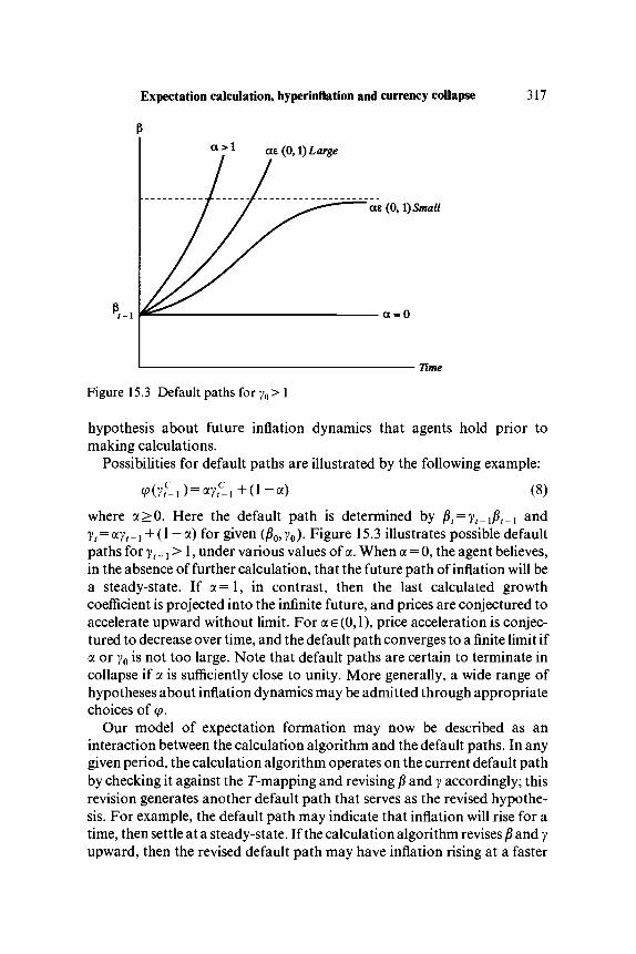
Expectation calculation, hyperinflation and currency collapse 317
ae (0,1) Large
ae (0,1) Small
Tune
Figure 15.3 Default paths for yo> 1
hypothesis about future inflation dynamics that agents hold prior tomaking calculations.
Possibilities for default paths are illustrated by the following example:
(y c i ) = oy,-i +(i - « ) (8)where a>0. Here the default path is determined by Pt = yt_iPt_l andyt = cnyt_x + (\ — a) forgiven (P0,y0). Figure 15.3 illustrates possible defaultpaths for yt_ x > 1, under various values of a. When a = 0, the agent believes,in the absence of further calculation, that the future path of inflation will bea steady-state. If a = 1, in contrast, then the last calculated growthcoefficient is projected into the infinite future, and prices are conjectured toaccelerate upward without limit. For ae(0,l), price acceleration is conjec-tured to decrease over time, and the default path converges to a finite limit ifa or y0 is not too large. Note that default paths are certain to terminate incollapse if a is sufficiently close to unity. More generally, a wide range ofhypotheses about inflation dynamics may be admitted through appropriatechoices of cp.
Our model of expectation formation may now be described as aninteraction between the calculation algorithm and the default paths. In anygiven period, the calculation algorithm operates on the current default pathby checking it against the T-mapping and revising P and y accordingly; thisrevision generates another default path that serves as the revised hypothe-sis. For example, the default path may indicate that inflation will rise for atime, then settle at a steady-state. If the calculation algorithm revises P and yupward, then the revised default path may have inflation rising at a faster

318 George W. Evans and Garey Ramey
rate in the short run, and then settling at a higher steady-state. The agentmay continue to revise his hypothesis by performing further iterations, andthe total number of iterations he performs indicates how intensely helabours to form expectations.
As the final ingredient of our calculation framework, we must specifyhow many iterations of the algorithm an agent performs as a function of hisinformation at the start of a period. We will assume that the number ofiterations is determined by the initial inputs for a period, according to thefunction &c(/?°, y°) that maps initial inputs into the integers 0,1,...,«; kc iscalled the calculation decision rule (CDR).12 The CDR represents thedecision theoretic component of our framework, and it is possible to chooseit from among a wide range of possibilities. For example, a CDR might bechosen to satisfy some notion of individual optimality, or a simple rule ofthumb might be specified. In the next section we will investigate onepossible choice for the CDR.
The model is completely determined once a CDR is specified, and we maydefine solution paths as follows. The sequence {($f,yf)}?=\ is a calculationpath (CP), relative to initial inputs (/??,y?), if for all /: (1) (Pf,yf) isdetermined by performing kc(P®,y®) iterations from the initial inputs(Pn 7/° )> a n d (2) (Pn 7/°) is formed from (f}f_ Uyf-X) using the input functions(7). The realized inflation path associated with a CP is determined by
Optimal calculation decision rules
Optimality criterion
We have defined solutions to the model relative to a given specification ofthe CDR, and further analysis now hinges on how the CDR is specified. Itseems plausible to suppose that the CDR would incorporate some balanc-ing by the agents of the costs and benefits of calculation. Agents' introspec-tive evaluation of their calculation problems may lead them to comparecosts and benefits; for example, agents might possess higher order calcula-tion technologies that allow them to compute a CDR that minimizesforecast errors net of calculation costs. Alternatively, agents may be led toan optimal CDR through some adaptive process. We will not investigateany particular selection process in this chapter, however; instead we willconsider a simple optimality criterion that may be interpreted as thelimiting outcome of some unspecified selection process.
Our optimality criterion begins with a specification of the costs andbenefits of calculation. In the hyperinflation model that we are considering,the benefits of calculation are associated with reductions in the losses from

Expectation calculation, hyperinflation and currency collapse 319
forecast errors. The following loss function expresses the losses fromforecast errors made in period t, where errors are reflected by the distancebetween actual and desired real balances:
-A-nt-A\y (9)Here nt+x is the agent's inflation expectation determined by the finaliteration of the algorithm in period t. We assume that h satisfies /*(()) = 0,/*'>() and/*">().
Calculation is assumed to be costly in terms of both time and resources.The time cost of calculation is reflected by the assumption that no morethan n calculations may be made in any period. Further, the resource cost ofmaking k < n calculations, expressed in the same units as the loss function /z,is given by ck. We assume that c0 = 0 and ck > ck_ { for k <n.
A CDR is optimal from an agent's point of view if it minimizes the lossesfrom forecast errors net of calculation costs, given the calculation decisionsmade by other agents. For simplicity, we will assume that agents areconcerned only with current period net losses, i.e. future losses are fullydiscounted.13 Further, we assume that agents take account only of thecurrent period calculations of other agents, and not the calculations thatother agents make in future periods. The latter restriction is needed topreserve consistency with agents' cognitive limitations as expressed by thecalculation algorithm: in period t, the algorithm incorporates the T-mapping for period t + 1 only, but future calculations depend on the T-mapping for periods t + 2 and beyond. Thus any procedure that agentsmight use in period t to check the future calculations would have to employstructural information that is unavailable according to the originalalgorithm.
With these restrictions, our optimality criterion takes the following form.Let nt+ j be calculated from the initial inputs j8,°, y,° for each possible numberof iterations k = 0,1,...,«. The net loss associated with k iterations is givenby (9) minus ck, where nt+ {in (9) is replaced by T(Jtf,yffif) (recall that /?,cand yf are the final period t outputs along the CP). Thus the calculatedinflation rates are compared to the inflation rate that would be realizedgiven the inflation expectations iit+ {= j3,c and nt+2 = yffif that other agentshold in period t\ this constitutes the best forecast of nt+ {that can be formedbased on other agents' period t calculations. According to this criterion, thebest forecast would be obtained by performing one more iteration than dothe other agents, i.e. by staying 'one step ahead of the pack'. Expectationformation can be interpreted as a 'calculation race', in which agents striveto get ahead of their rivals, but are unable to do so since agents calculatesimultaneously and have equal calculation abilities. An optimal CDRchooses kc to be a Nash equilibrium of this calculation race.

320 George W. Evans and Garey Ramey
More formally, our optimality criterion is expressed as follows. Wesuppress the time subscripts, since the criterion depends only on the initialinputs and not on the particular period. Let the best response functionkM(k) be defined by:
kcis said to be optimalifkc(P°,y0)ekM(kc(p°y)) for all j?°,y°. Existenceof an optimal CDR is considered in Proposition 1, whose proof is given inthe appendix:
Proposition 1: If x\l/(x\/3,y)>0 for all x,/?,y, then there exists anoptimal CDR.
Proposition 1 establishes existence of optimal CDRs under the assump-tion that y is never revised in the opposite direction as /}, which constitutes aweak version of the acceleration property discussed on p. 314. This assump-tion assures that calculation trajectories possess monotonicity of the formexhibited in figure 15.2, and monotonicity is needed in turn to establishexistence of fixed points of kM.
Optimal CDRs for a particular specialization of the model are depictedin figure 15.4.14 The maximum number of iterations per period in thisexample is « = 3, and the cost per calculation is constant at c k — ck_x = 1.Figure 15.4a gives the CDR that minimizes the number of iterations amongall optimal CDRs, while Figure 15.4b gives the CDR that maximizes thenumber of iterations; the structure that underlies the two figures is identical.This illustrates the scope for multiplicity of optimal CDRs, which emergesas a consequence of the strategic complementarities that are inherent in thecalculation race. Note that for sufficiently high /?° and y°, the agentscalculate nt+l>nt+l, and collapse then occurs in period t.
As mentioned above, our notion of optimal CDRs sidesteps the issue ofhow agents actually determine the optimal CDR, and instead movesdirectly to a limiting selection. In essence, we have replaced the initialrational expectations hypothesis with a rationality hypothesis that isimposed after one level of calculation. While this procedure does not createany difficulties from the purely logical standpoint, as argued by Lipman(1991), it does involve a certain philosophical inconsistency. We respond tothe latter criticism in two ways. First, our optimal CDR is meant to capturethe intuitive and empirically meaningful notion that agents balance costsand benefits in making their calculation decisions. The reasonableness ofour specification relative to the alternative hypotheses of rational expec-tations and passive adaptation becomes a testable issue, and we argue

Expectation calculation, hyperinflation and currency collapse 321
(a) 1Collapse
(b)
1.5 -
1Collapse
Figure 15.4 Optimal CDRs(a) Minimum calculation (b) Maximum calculation
below that our theory receives strong empirical support.15 Second, theoptimal CDR may be regarded as a tractable first step in the modelling ofcalculation behaviour, and the more complex problem of explicitly model-ling the CDR selection process is appropriately left for future work.16

322 George W. Evans and Garey Ramey
Behaviour of calculation paths under optimal calculation decision rules
In this subsection we consider the long-run behaviour of CPs that aregenerated by optimal CDRs. The main result is that under mild restrictionson the calculation algorithm and input functions, when calculation costsare small CPs can settle only at points that are either close to steady-stateREE or are in the collapse region. We also consider the stability of the highinflation and low inflation steady-state REE. Readers may ignore thissubsection without loss of continuity.
Some new terminology is needed to describe the asymptotic behaviour ofCPs. Suppose Dt = D and ftt+x — ft for all t. For a given neighbourhood TV ofthe (/?, y) plane, we say that a CP terminates in TV if there exists a time Tsuchthat (Jif, yf) e TV for all t>T.A point (p, y) with P < ft is a terminal point if forany neighbourhood TV containing (/?, y), there exists a CP that terminates inTV. The collapse outcome is said to be a terminal point if there exists a CPthat terminates in collapse. Thus terminal points give the outcomes atwhich CPs can settle.
Proposition 2 provides a characterization of the set of terminal points,under weak restrictions on the input function cp. The proofs of this and thefollowing propositions are given in Evans and Ramey (1992b).
Proposition 2: Let \jj and cp be C1 functions, and suppose:(a) x\l/(x\P,y)>OforaHx,P,y;(b) (p(PA)=l for all P;(c) 0<<p2(jS,y)<lforallj3,y.17
Then for c{<h(D), the set of terminal points is characterized as follows.(I) If D< Z), then the terminal points are the collapse outcome together
with:
where NL and Nv are closed subintervals of (0, ft), possibly overlap-ping, with 7iLeint{7VL}, Ti^eintlA^}. The intervals become strictlysmaller as cx declines, and:
lim NL = {nL}, lim N^in^.
(II) If D > D, then the terminal points are the collapse outcome togetherwith:
where for cx sufficiently close to h(D), NM is a closed subinterval of(0,7f). NM becomes strictly smaller as cx declines. If Z> = Z>, then NM

Expectation calculation, hyperinflation and currency collapse 323
Collapse
(b)
Figure 15.5 Set of terminal points(a)D<D(b)D>D
shrinks to a single point as cx approaches zero, while for D>D, NM isempty for cx sufficiently small.18
The set of terminal points characterized by Proposition 2 is illustrated infigure 15.5. Observe that given our conditions on cp, all non-collapse ter-minal points must have y = 1; in particular, condition (b) ensures that if

324 George W. Evans and Garey Ramey
agents believed they were in a steady-state in the preceding period, then thedefault path continues to reflect this belief in the current period. It followsthat agents must recognize that they are in a steady-state if the economycomes to rest at some point. CPs can settle only at points that are approx-imately REE when the cost of a single calculation is low, and the set of ter-minal points shrinks to the steady-state REE as this cost approaches zero.
For larger calculation costs, in contrast, there exist terminal points thatare not near any steady-state REE. In particular, non-collapse terminalpoints exist in the high deficit case, despite the fact that there are no non-collapse steady-state REE. At terminal points of the latter form, flf may beclose to nt+l, so that forecast errors are small. Thus non-existence ofnon-collapse steady-state REE does not rule out the possibility of 'near-rational' steady-states associated with non-negligible calculation costs.
The condition cp2 < 1 ensures that in projecting the future path ofinflation, agents reduce at least slightly the degree of price accelerationimplied by the previously calculated y. As example (8) illustrates, this isneeded to ensure that agents are allowed to entertain conjectures ofconvergent inflation paths when y i=-1. It is interesting to note that thecondition eliminates 'hyperdeflationary' paths in which flf converges tozero; essentially, the existence of such paths requires that the default pathsreflect an extremely large degree of downward price acceleration.19
We turn now to the issue of the stability of terminal points, and inparticular we are interested in the question of which terminal points arerobust to low calculation costs. Two related concepts of stability will beconsidered. The first concept is motivated by the standard notion of localstability: (/?, y) with /? < ft is said to be C-stable if, for any neighbourhood Mcontaining (/?,y), there exists a neighbourhood NaM such that thefollowing is true: for any specification of calculation costs, and for any(Pi,y?) eN, there exists a CP that terminates in M. Thus initial inputs thatare close to (/?,y) can give rise to CPs that remain close to (j3,y).
Our second concept is motivated by the usual notion of asymptoticstability: (/?,y) with /?<f is asymptotically C-stable if there exists Mcontaining (/?, y) with the following property: for all N containing (/?, y),there exists c > 0 such that for any (/??, y?) e M, all ensuing CPs terminate inTV if cx < c. This departs from C-stability by requiring that all CPs generatedby nearby initial inputs must become arbitrarily close to (/?,y) for suffi-ciently small calculation costs. Asymptotic C-stability is not stronger thanC-stability, however, since the latter does not impose any restrictions oncalculation costs.
Using Proposition 2, it is clear that (7CL,1) and (rc^l) are the onlynon-collapse points that can satisfy either definition under the givenconditions on cp. Proposition 3 further considers these two points.

Expectation calculation, hyperinflation and currency collapse 325
Proposition 3: Let \\J and cp be C1 functions that satisfy (a)-(c) ofProposition 2, and suppose D<D.(I) (TTL,1) is C-stable and asymptotically C-stable if the following ratio is
sufficiently small:20
(II) (nU9l) can be neither C-stable nor asymptotically C-stable.
Proposition 3 establishes that the high inflation steady-state REE fails tobe stable, in that there are arbitrarily close initial inputs giving rise to CPsthat lead away from the steady-state when calculation costs are low. Thelow inflation steady-state REE satisfies the stability criteria when^(OITT^I) , which measures the strength of the acceleration property near(TTL,1), is small in the sense stated in Proposition 3. Essentially, thealgorithm must not accelerate y away from (nu\) faster than the defaultpaths pull y in.21
Finally, although we will not pursue the details, it is worth noting that thecollapse state is stable in a certain sense. Consider the subregion of thecollapse region on which y > 1. Initial points sufficiently close to thissubregion, with yo> 1, will generate CPs that remain close to the collapseregion, and terminate in collapse if cx is sufficiently small. On the otherhand, the subregion with y < 1 can be regarded as unstable; initial expec-tations that lie close to the collapse region and below the ys curve do notgenerate CPs that remain close to the collapse region.
Examples of calculation paths
In this section we will consider some examples of CPs that demonstrate howour theory offers explanations for the empirical phenomena discussed in theIntroduction. The examples are calculated using the specifications of ^ andcp given in (6) and (8).22 Costs per calculation are constant at ck — ck_l = c, upto the per period limit of n. The examples consider various values of c and n.Calculation decisions are determined by optimal CDRs, as defined in thepreceding section; in all cases we select the optimal CDRs that maximize thenumber of iterations of the algorithm.
Permanent deficit increase: low deficit case
Suppose that the economy begins in a long-run steady state at D = 0, withnt = nL= 1 for t< 1. At the beginning of period 1, the governmentannounces a permanent increase in the deficit to D = 1.768, which is to beginat t= 3. This deficit level is associated with a new low inflation steady-state

326 George W. Evans and Garey Ramey
Table 15.1. Permanent deficit increase: data for low-deficit case
n=\,t
knt+\
Ptyc
t
/i = 3,t
k
fityc
t
«=i,t
knt+\
Ky<
c = 0.011
01.24411
c = 0.011
01.4411
c=\1
01.24411
2
12.1231.5471.054
2
32.2342.0851.089
2
11.8731.5471.054
3
12.0861.8691.042
3
02.0392.271.045
3
01.8701.6321.027
4
12.0852.0161.025
4
22.0342.1681.013
4
01.8681.6761.014
5
02.0592.0661.012
5
12.0092.1161.003
5
01.8671.6991.007
6
02.0592.0911.006
6
12.0312.0660.999
6
01.8671.7111.003
7
02.0082.1041.003
7
02.0312.0630.999
7
01.8671.7171.002
8
12.0292.0590.999
8
02.0312.0621.000
8
01.8671.7201.001
9
02.0292.0571.000
9
02.0312.0611.000
9
01.8671.7211.000
of nL = 2. Table 15.1 and figure 15.6 summarize the calculation behaviourand inflation paths elicited by the policy beginning in period 1.
Initial inputs in period 1 are given by ^ = yi = l. Note from table 15.1that announcement of the policy generates no effect in period 1; agents aremaking calculations of period 2 inflation, and these calculations are notaffected by a deficit increase that occurs in period 3. Thus agents have noincentive to calculate, and final outputs remain at the initial input levels,with nl = 1.
Now consider the calculation decisions in period 2. Agents want tocalculate TT3, and since D3 > 0 the algorithm gives outputs $\ > f$l, y\ > y%.Iteration of the algorithm leads agents to revise n3 upward, which reducesdesired money holdings and increases the period 2 inflation rate. Thuscalculation in period 2 generates an inflation reaction one period in advanceof the policy change. This is consistent with Marimon and Sunder's (1988,1991) finding that anticipated policy changes led to significant reactionsonly in the periods immediately preceding the changes.
In this case, the one-period ahead anticipation effect emerges from theone-period forecast horizon of the algorithm. More generally, the degree of

Expectation calculation, hyperinflation and currency collapse 327
(a)
1.05
0.95 -
2.5
(b)
1.5
1 2 3 4 5 6 7
Figure 15.6 Permanent deficit increase: low deficit case(a) Trajectories of CEPs (b) Inflation pathsO « = 1 , c = 0.01 A « = 3, c = 0.01x / i = l , c=\ • Pathof7r L
anticipation would depend on the length of the forecast horizon built intothe algorithm, which in turn would reflect the cognitive abilities of agents. Itis important to note that such limited anticipation effects are inconsistentwith either rational expectations, which predicts immediate reaction toannounced policy changes, or passive adaptive learning, which posits thatreactions occur only after the changes are implemented.23
In the case of n= 1, c = 0.01, agents calculate again in periods 3 and 4, atwhich point expectations are sufficiently accurate to dissuade them fromcalculating in period 5. The default path then carries the agents toward aterminal inflation rate in excess of 2, and by period 8 the default path
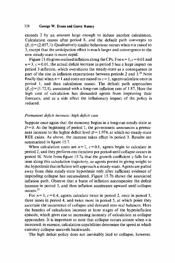
328 George W. Evans and Garey Ramey
exceeds 2 by an amount large enough to induce another calculation.Calculation ceases after period 8, and the default path converges to(/?, y) = (2.057,1). Qualitatively similar behaviour occurs when n is raised to3, except that the anticipation effect is much larger and convergence to thenew steady-state is more rapid.
Figure 15.6b gives realized inflation along the CPs. For n = 1, c = 0.01 andn — 3, c = 0.01, the actual deficit increase in period 3 has a large impact onperiod 3 inflation, which overshoots the steady-state as a consequence inpart of the rise in inflation expectations between periods 2 and 3.24 Notefinally that when n = 1 and costs are raised to c = 1, agents calculate once inperiod 1, and then calculation ceases. The default path approaches(P,y) = (1.72,1), associated with a long-run inflation rate of 1.87. Here thehigh cost of calculation has dissuaded agents from improving theirforecasts, and as a side effect the inflationary impact of the policy isreduced.
Permanent deficit increase: high deficit case
Suppose once again that the economy begins in a long-run steady-state atD = 0. At the beginning of period 1, the government announces a perma-nent increase to the higher deficit level D= 1.974, at which no steady-stateREE exists. As above, the increase takes effect in period 3. Results aresummarized in figure 15.7.
When calculation costs are n= 1, c = 0.1, agents begin to calculate inperiod 2, and they perform one iteration per period until collapse occurs inperiod 10. Note from figure 15.7a that the growth coefficient y falls for atime along this calculation trajectory, as agents persist in giving weight tothe hypothesis that inflation will approach a steady-state. Agents are pulledaway from their steady-state hypothesis only after sufficient evidence ofimpending collapse has accumulated. Figure 15.7b shows the associatedinflation path. Observe that a burst of inflation accompanies the deficitincrease in period 3, and then inflation accelerates upward until collapseoccurs.25
For « = 3, c = 0.4, agents calculate twice in period 2, once in period 3,three times in period 4, and twice more in period 5, at which point theyascertain the occurrence of collapse and demand zero real balances. Herethe benefits of calculation increase at later stages of the hyperinflationepisode, which gives rise to increasing intensity of calculation as collapseapproaches. It is important to note that collapse occurs sooner when n isincreased; in essence, calculation capabilities determine the speed at whichcurrency collapse unravels backwards.
The high deficit policy does not inevitably lead to collapse, however.

Expectation calculation, hyperinflation and currency collapse 329
(a)
Figure 15.7 Permanent deficit increase: high deficit case(a) Trajectories of CEPs (b) Inflation pathsO n = \ , c = 0A A n = 3,c = 0 A * n = \ , c = \
When calculation costs are increased to n= l,c= 1, agents perform oneiteration each in periods 2 and 3, and then cease calculation. After this pointexpectations are sufficiently close to rational that there is insufficientincentive to continue calculation; the CP then evolves toward the terminalpoint (j8, y) = (2.43,1), and the inflation rate reaches a long-run steady-stateat 2.60. The occurrence of such a steady-state clearly distinguishes ourapproach from rational expectations and passive adaptive learning, in thatboth of the latter predict that no non-collapse steady-state is possible in thehigh deficit case.
Moreover, steady-states in the high deficit case are most likely to occur
330 George W. Evans and Garey Ramey
where expectations are nearly rational, i.e. in the neighbourhood of thecurve ys. In fact, Marimon and Sunder did observe steady-states in highdeficit cases where no steady-state REE existed, and these steady-statesarose precisely where expectation errors were smallest. Our calculationframework provides a simple explanation for this anomalous laboratoryfinding: subjects' expectations were sufficiently close to rational thatrethinking them was not worth the effort.26
Policy reversal
We close by considering a slightly more complex policy experiment. Theeconomy begins in a long-run steady-state at a deficit level of D = 1.768. Inperiod 1 it is announced that the deficit will be raised to D = 1.974 in period3, and kept at this level until some later period, at which time it will berestored to Z) = 1.768. Figure 15.8 illustrates the inflationary effects forvarious policy reversal dates.
In figure 15.8a, in which calculation costs are n— 1, c = 0.01, collapseoccurs in period 10 in the absence of policy reversal. When the policy isreversed at t = 5, there is a relatively small and transitory inflationary effect,with the inflation rate peaking at 2.81 in period 3. Reversal at t = 8 generatesa higher peak inflation rate of 3.53 in period 6. In period 7 agents anticipatethe policy reversal in period 8, and begin calculating downward expectationrevisions.
If policy reversal is delayed too long, it becomes impossible to avertcurrency collapse. Consider the effects of a reversal at f = l l . Agentscalculate in periods 2 through 9, revising upward their conjecture of theinflation path. In period 10, the anticipated deficit reduction makes thedefault path more accurate, and agents do not calculate. In period 11,however, the default path has advanced sufficiently far toward collapse thatcalculation once more revises the path upward, despite the lower deficitlevel. Continued upward acceleration then drives the economy to collapsein period 13. This indicates that the timing of policy reactions to hyperinfla-tionary episodes may be crucial, in that collapse may become inevitableonce expectations have been allowed to pass a critical point.
Figure 15.8b illustrates the effects of policy timing under a fastercalculation technology, with n = 2. Now collapse in period 6 becomesinevitable when policy reversal is delayed past t = 7. It follows that the costto policy-makers of delay increases when agents can calculate more rapidly.
Conclusion
This chapter has developed a theory of expectation formation in hyperin-flationary environments, in which expectation revisions are tied explicitly

Expectation calculation, hyperinflation and currency collapse 331
(a)10
8
6
4
2
01 2 3 4 5 6 7 8 9 10 11 12 13 14
10
(b)
0 O O O O Q O
1 2 3 4 5 6 7 8 9 10 11 12 13 14
Figure 15.8 Policy reversal
O Reversal at t = 5 A Reversal at t = 8 x Reversal at t= 11(b)/i = 2,c = 0.01O Reversal at t= 5 A Reversal at t = 6Reversal at t = 7 implies collapse at r = 5
to agents' trade-offs between losses from inaccurate forecasts and the costsof calculating expectation revisions. Our theory posits a particular form foragents' expectation calculation algorithms, in which they use a true modelof the economy to guide their calculations. We show that a wide variety ofeconomic phenomena can be explained in terms of agents' capabilities andincentives to calculate expectations.
Our theory explains how, in cases of unsustainable budget deficits, apattern of accelerating inflation followed by currency collapse arises

332 George W. Evans and Garey Ramey
naturally from agents' increasing incentives to calculate expectations as thehyperinflationary episode unfolds. Moreover, laboratory findings of one-period ahead anticipation effects, rapid adjustment to new steady-states,and convergence to near-rational outcomes when steady-state REE do notexist, which are difficult to understand in terms of either rational expec-tations or least squares learning, are easily comprehended when agents'capabilities and incentives to calculate expectations are taken into account.
Finally, our approach has important implications for policy, particularlyfor policy reversibility. When calculation behaviour is considered, thetiming of policy shifts can be crucial not only for the transitional dynamics,but for whether currency collapse can be averted as well.
This chapter has focused on a particular relatively simple specification ofthe calculation technology, but clearly our framework can be extended inmany directions:
Extensions of the calculation algorithmThe algorithm might be based on a model of economic structure that differsfrom the true structure, where the difference would reflect incompleteknowledge on the part of agents. The algorithm could incorporate a longerforecast horizon, as discussed on pp.315-16, and forecast rules rather thanpoint forecasts might be calculated. The agents could be required to engagein costly calculation of best responses to expectations as well as theexpectations themselves (Marimon and Sunder, 1988, 1991, find experi-mental evidence that agents do not fully optimize their money holdings,given their expectations).
Dependence of the algorithm on the information setIn the specification employed by this chapter, the only aspect of theinformation set that affects calculation is an agent's own previous calcula-tions. This has allowed us to make a sharp distinction between ourapproach and that of passive adaptive learning. Our framework can inprinciple be modified, however, to allow a rich dependence betweeninformation and calculation. Calculation behaviour might depend on pasteconomic data, as well as past calculations, via the input functions, theCDRs, or direct revisions of the structural model or calculation procedure.For example, agents might compare past calculated inflation rates withrealized rates, with larger discrepancies triggering more intensive calcula-tion. An average of past inflation rates may be updated and used to modifythe initial input should agents choose to calculate. These and otherextensions would make possible a natural combination of passive adap-tation and active cognition.27

Expectation calculation, hyperinflation and currency collapse 333
Determination of the CDRAn adaptive process could be introduced that directly adjusts the CDRs inresponse to their success at minimizing net losses, e.g. some form ofevolutionary adaptation might be specified. Optimality of the CDR wouldthen arise only gradually, if at all.
Our overriding goal has been to establish a general framework foranalysing expectation formation behaviour that allows agents to engage ina process of active cognition with respect to the economic environment, butplaces inherent limitations on their cognitive abilities in terms of restric-tions on the calculation technology. We believe that the framework andresults of this chapter, and the possible extensions outlined above, areindicative of the scope for this approach to capture a rich variety ofexpectation formation behaviour.
Appendix
Proof of Proposition 1: Note first that, for all k:
\ k k k \yon-p°l (Al)To see this, suppose T(P°,y\P°)> P°. Then (5a) and (5b) give pl>p° andyl>y°, where the latter invokes the acceleration property. Further, sinceT(fi,yP) is strictly increasing in p and y, we have T(P\ylpl)>T(p°,y°p°)= Pl. The inequality extends to all k by induction, and the argument applies
V 0 0
Note next that kM{k) is non-decreasing in k, that is, k<k\ kvekM(k),kwekM(k') imply kv<kw. Suppose T(p°,y°P°)> p° and choose &v = maxkM(k), k'>k. By definition we have, for all kx<kv:
h(K\(pkxya-T(pkypkya\)+ckx>h(K\(pkvya
-T(pkypkya\)+ck,Using (Al) it follows that pk'>pk and / ' > / , and so T(pk\yk'pk>)> T(pk,ykpk). Similarly, we have pkx<pkv. Define the following:
B=(pkvya-T(pkypkya
C=T(pk,ykpk)-a-T(Pk\yk'pk')-a.Note that A > 0 and C> 0. Now (A2) may be written:
h(K\B\)>ckv-ckx>0 (A3)which implies \A + B\ > \B\; combining this with A > 0 implies A + B> 0. Tohave kx$kM{k') it is sufficient that:

334 George W. Evans and Garey Ramey
+ B+C\)-h(K\B+C\)>ckv-ckx. (A4)
If B + C>0, we may differentiate the left-hand side of (A4) with respect to Cto obtain:
+ B+C))-h'(K(B+C))]K>0
while if B+ C< 0, the derivative becomes:
[h1(K(A + B+ C)) + h''(- K(B+ C))]K>0.
Thus (A4) follows from (A3) and C> 0.Finally, fix k = n. If n ekM(n), then we are done. Otherwise, kv < n for all
kvekM(n). Now consider k = n— 1. Again we are done if n— 1 ekM(n— 1).Otherwise, note that we cannot have nekM(n-\), or we would havenekM(ri) due to the fact that fcMis non-decreasing, and so we would havefinished in the first step. Thus if n— 1 $kM(n— 1), then kv<n—\ for allkvekM(n~ 1). Proceeding by induction, for each k we have kekM(k) orkv<kfor all kvekM(k), and at = 0 we must have 0e&M(0). •
Notes
Part of this chapter was originally included in 'Expectation Calculation andMacroeconomic Dynamics' STICERD Discussion Paper, TE/89/202, LondonSchool of Economics (1989). Earlier versions were presented at the NBERConference on Economic Fluctuations in Cambridge, MA (October 1991), theEconomic Science Association meetings in Tucson (October 1991), the OFCEconference in Paris (January 1992), and the Econometric Society North AmericanWinter Meetings in New Orleans (January 1992). We have benefited from numerouscomments, and we are particularly grateful for the comments and criticisms of JohnConlisk, Charles Goodhart, Herschel Grossman, Rudolfo Manuelli, Neil Rankin,Mark Salmon and Michael Woodford. The authors are responsible for all errors.
1. Historical evidence is given in Bental and Eckstein (1990), who also explicatethe difficulties of duplicating the historical pattern in a rational expectationsequilibrium.
2. In experimental environments with unchanging deficit levels, Marimon andSunder (1993) did find some agreement between subjects' forecasts and leastsquares predictions.
3. Note that agents can observe Pt and Pt-]9 and thus they know nt, when theychoose their period-r money holdings. The future realization nt+u whichdepends on Pt+l, is what agents are seeking to forecast in this model.
4. Essentially, currency becomes worthless once the government defaults. Equiva-lently, we can view the government as issuing infinite amounts of currency in thecollapse period, which drives Pt to infinity. Alternative assumptions arepossible for the period after default, and these might modify calculationbehaviour in the periods immediately preceding default.
5. Bental and Eckstein (1990) show that to obtain an accelerating pattern of

Expectation calculation, hyperinflation and currency collapse 335
inflation that terminates in an anticipated stabilization requires not high butlow (i.e. sustainable) deficits in the prestabilization period, combined with anappropriate shift in taxes (in addition to any cut in government consumption) atthe stabilization date itself. Another possible route for reconciling rationalexpectations with historical hyperinflation experience might be to incorporate aregime shift of uncertain existence or timing. See Flood and Garber (1980a) foran example of this kind of approach in a model with an exogeneous moneysupply process.
6. When k = 0 and 7°= 1, the calculation algorithm is equivalent to the notional-time process of expectational stability used in Evans (1985) to analyse stabilityof steady-state REE. Here expectational stability becomes an algorithm forcalculating expectations in real time.
7. The qualitative features shown in figure 15.2 hold for a < 1, which generates theinitial convex region of the ys curve, and ke(0,\), which yields the concavecalculation trajectories.
8. Calculating a fixed point of the algorithm in period / would not imply that allforecast errors are eliminated, however, since the algorithm does not incorpor-ate structural changes that occur beyond the forecast horizon, nor does itaccount for calculations that are made in future periods.
9. One could further extend the algorithm by allowing the choice of Hto be part ofthe algorithm; more generally, agents might be allowed to choose betweencompeting algorithms. We leave the analysis of the more general and complexcases for future work. Other possible extensions of the calculation frameworkare discussed in the Conclusion.
10. A number of alternative possibilities are discussed in the Conclusion.11. The default path in Evans and Ramey (1992a) is simply $ = Pf-\\ agents in that
model seek to predict only current inflation, and the calculation algorithm has asingle input and output.
12. It is also possible that the CDR would depend on other variables, such as pastobserved inflation rates; such possibilities are discussed further in the Conclu-sion (pp.332-3).
13. Discounting of future losses is considered in Evans and Ramey (1992a).14. This specialization puts a = 0.5, K=5, D= 1.768, \jt is given by (6) with k = 0.1,
the loss function is h(z) = 3z2, w = 3, and ck — ck_l = \ for k— 1,2,3.15. Recent experimental work of Smith and Walker (1993a, 1993b) on decision
costs gives further support to the notion that calculation behaviour derivesfrom a consistent balancing of benefits and costs: undergraduate experimentalsubjects were found to commit smaller decision errors when the payments for agiven experiment were scaled upward. Here the benefits of calculation areincreased, while the costs are presumably constant across subjects, and theresults are consistent with the notion that calculation becomes more intensive.
16. In a single-agent model, Conlisk (1988) takes a similar approach to optimaldecisions under bounded rationality, and he gives further discussion of thejustifications for this approach.
17. cp2 denotes the derivative with respect to the second argument, y.18. For cx >h(D) the set of terminal points may have other forms. In particular, if

336 George W. Evans and Garey Ramey
a>\ the intervals may be of the form [/?,7i), i.e. there are terminal pointsarbitrarily close to the collapse region. Further, in the low deficit case a thirdinterval of this form may be added to NL and Nu.
19. The condition also serves to rule out cases in which the input functions andcalculation algorithm exactly offset one another from period to period, which itdoes by ensuring that current calculations have a persistent effect on the defaultpath.
20. if/] denotes the derivative with respect to the first argument, x.21. Our findings of potential stability of the low inflation steady-state and
instability of the high inflation steady-state are in agreement with Marimon andSunder's experimental results; see especially Marimon and Sunder (1993).
22. Values for the parameters a, K and k are as in n. 14 above, and also a = 0.5.23. Limited anticipation could arise even if the calculation algorithm incorporated
a very long forecast horizon, provided that calculation costs are not too small.24. To understand this overshooting effect, let us rewrite (1) as Amt + mt-x(nt
— \)jnt = D, where mt = HJPt. The second term on the left-hand side is theinflation tax component of seigniorage, while the first term is an additionalsource of seigniorage generated by the willingness of agents to hold higher realbalances. When fit > Pt_ ls Amt is negative, and a higher inflation tax is needed tofinance D.
25. Although behaviour is describable as a speculative bubble in this instance, it isnot an explosive REE path like those described by Obstfeld and Rogoff (1983),since the adjustment is driven by calculation behaviour rather than REEdynamics. This indicates a source of price level bubbles that has not beenaddressed by standard empirical tests along the lines developed, for example, byFlood and Garber (1980b).
26. These near-rational steady-states differ from the near-rational equilibria ofAkerlof and Yellen (1985a), as well as the steady-state outcomes described intable 15.1, in not being close to any steady-state REE.
27. Further, if agents are heterogeneous, then the information flows available to anagent may include the calculations of other agents. This would generatecalculation externalities, as discussed in Evans and Ramey (1992a).

16 Menu costs and aggregate pricedynamics
Alan Sutherland
Introduction
The idea that small costs of adjusting prices can create significant nominalrigidities is now a well known result in macroeconomics. The basicimplications of menu costs are easily derived and demonstrated in a simplestatic model of a monopoly firm (as in Akerlof and Yellen, 1985b; Mankiw,1985). However, there are now a number of studies which generalize thisanalysis, first, to consider the dynamic behaviour of an individual represen-tative firm (Sheshinski and Weiss, 1977, 1983), and secondly, to considerthe dynamic behaviour of the aggregate price level when firms are hetero-geneous (Caplin and Spulber, 1987; Caplin and Leahy, 1991). This chapterbrings together the main results of this literature and presents them in aunified framework which is accessible to non-specialist readers.1
The chapter begins by deriving and explaining a dynamic menu costmodel of an individual firm. In this context 'dynamic' means that the firmaims to maximize the discounted value of its profit stream while experienc-ing serially correlated shocks to the demand for its product. The firmtherefore faces an ongoing price adjustment problem such that at everyinstant it must decide whether and by how much it should adjust its pricelevel. This contrasts with the models of Akerlof and Yellen (1985b) andMankiw (1985) where the firm experiences a single shock and is onlyconcerned with maximizing profits within the current period. In the firstsection it is shown how, in the dynamic model, a firm chooses optimaltrigger values of the deviation of its price level from the frictionlessoptimum. While the value of this deviation is small enough to be betweenthe trigger points the firm holds its price fixed. But when the deviation hitsone of the trigger points, prices are adjusted by a discrete amount. The basicinsight of the static models therefore survives in a dynamic framework.
If all firms are identical and face identical shocks to demand it is obviousthat the nominal stickiness displayed by each individual firm will also bedisplayed by the aggregate price level. But if firms are heterogeneous in
337

338 Alan Sutherland
some way, so that each firm is potentially at a different position relative toits price trigger points, it becomes less clear that the menu cost effect willsurvive at the aggregate level. When firms are heterogeneous it becomestheoretically possible for there always to be some firms at or near theirtrigger point so that any aggregate shock (such as a monetary shock) willalways trigger some price adjustment. To investigate this issue it clearlybecomes necessary to construct a framework where there are many firmssubject to menu costs in the presence of both idiosyncratic and commonshocks. Such a framework is constructed in the second section of thechapter.2
The third and fourth sections of the chapter then use this framework toanalyse two important and contrasting cases. In the first case (due to Caplinand Spulber, 1987) the shocks the firms face are all of the same sign so thatprices move in only one direction. It is shown that, in this case, firms aredistributed in such a way that any common shock (i.e. money supply shock)induces just enough firms to change their prices to keep the real moneysupply constant. In other words, the stickiness evident in prices at the levelof the individual firm is lost at the aggregate level and monetary shocks areneutral despite the presence of menu costs. The assertion that menu costs atthe individual firm level must give rise to nominal stickiness at the aggregatelevel is thus revealed to be a 'fallacy of composition'.
The fourth section, however, considers an alternative case (due to Caplinand Leahy, 1991) which shows that this fallacy of composition is by nomeans a general result. The crucial difference in this case is that shocks canbe either positive or negative. This apparently innocuous change to thestructure of the model is sufficient to produce a very different distribution offirms. The equilibrium distribution of firms is such that there need not beany firms close to a price level trigger point. It is therefore possible for thereto be a monetary shock which does not induce any price adjustment. Thusaggregate price inertia is generated and money is non-neutral.
Dynamic optimization and the individual firm
In this section a dynamic model of an individual firm's pricing decision isconstructed. The firm's problem is analysed in a continuous-time stochasticframework where the shocks hitting the firm take the form of a 'compoundPoisson' process.3 The compound Poisson process has the advantage that itencompasses both the one-sided and two-sided cases. Thus, by a suitablechoice of parameter values, it is possible to generate the Sheshinski andWeiss (1983) case where the firms' optimal price only ever rises, and theCaplin and Leahy (1991) case where the firm's price can both rise and fall.4
Suppose that an individual firm faces a stochastic demand schedule such

Menu costs and aggregate price dynamics 339
that, in the absence of adjustment costs, its profit maximizing price, /?*,follows a compound Poisson process.5 Thus if/?* is the profit maximizingprice at time / then p* at time t + dt is given by the following
!
pf — e with probability ccMtpf with probability (l-Mt) (1)
pf + s with probability (1 — (x)Mtwhere 0 < a < 1 and where the innovation, e, is exponentially distributedwith density given by ye ~yE (8 is therefore non-negative). The average drift(per unit time) in/7* is given by >l(2a - l)/y. And the variance (per unit time)is 21/y2.
The one-sided and two-sided cases are generated by suitable choice of theparameter a (which has a central role in determining the degree of drift inthe/?* process). If a = 1 the process is asymmetric and prices only ever rise.This corresponds to the case analysed by Sheshinski and Weiss (1983).6 If,on the other hand, a = 1/2 the /?* process is exactly symmetric and priceshave no tendency to either rise or fall. This is the model of an individual firmthat corresponds to the aggregate analysis of Caplin and Leahy (1991).
Denote the actual price that the firm sets at time t bypt and define xt to bethe deviation between the actual and optimal price, i.e. xt—pt—pf. Thus,between price changes x follows the following process
{ xt-8 with probability (1 - a)Mtxt with probability (1 - Mi) (2)
xt + e with probability ccMtAssume the firm's instantaneous profit function is quadratic in x in theregion of maximum profits such that
nl=-b[p-pf]2=-b[xl]2 (3)where b is a fixed parameter. Here 771 is the difference between the actualflow of profit that is earned at time t and the maximum that could be earnedif pt is set equal to pf. As pt moves away from pf in either direction 77,becomes negative.
The firm has to pay a menu cost of k every time the price level is altered.The firm's objective is to maximise the discounted value of profits net ofadjustment costs. The firm's objective at time t is therefore to maximize Wtwhere Wt is given by the following
(4)

340 Alan Sutherland
where 3 is the firm's discount rate and Et is the expectations operatorconditional on information available at time t.Cx = k if prices are adjustedat time T, otherwise CT = 0. By substituting from (3), (4) can be rewritten as
00
W, = E, | f [ - bx] - Ct]e "^-«>rfr j . (5)
The firm's problem is to choose x at each moment of time in order tomaximize Wt.
The optimal form of rule for the firm is to choose upper and lower triggerpoints for price changes, denoted u and /, and upper and lower returnpoints, denoted U and L. Thus when x reaches the value u the firm adjustsits price (and therefore incurs the lump sum cost k) so as to return x to U.Likewise at / the price level is adjusted so as to return x to L. Proving thatsuch a trigger point rule is optimal within a wider class of rules is a difficultproblem which is not tackled here. For the purposes of the exerciseconducted below it is taken as given that a rule of this form is optimal andthe procedure for deriving the optimal values of w, /, U and L is outlined. Itshould be noted, however, that this rule is sufficiently general to encompassa number of important special cases. In particular the case where the firmcontinuously maintains its price at p* can be represented asu = l=U=L = 0. The fact that this does not turn out to be optimal for a firmthat faces menu costs shows that price stickiness is not an artefact of theassumption that a trigger point rule is followed.
The procedure for deriving the optimal values of u, /, U, L involves firstderiving an explicit expression for the value of the firm's objective function.It is possible to deduce from the structure of the model that Wt will be somefunction of xt9 i.e. Wt= V(xt).7 Consider a small interval of time, dt, duringwhich price adjustment does not take place (i.e. l<xt<u and l<xt+dt<u).The function V{) satisfies the following8
V{xt)= ~bx*dt + {\-8dt)Et[V{xt+dt)]. (6)The definition of the process followed by x allows the last term of this to beexpanded to yield
V(xt)= -bx?dt + (l-5dt)Ul-(x)ME[V(xt-s)]l. (7)l JThe first term in the large bracket is the value of the objective function att + dt if there is no change in x multiplied by the probability of there beingno change. The second term is the expected value of the objective function
Menu costs and aggregate price dynamics 341
given that there is a negative jump in x multiplied by the probability of anegative jump. The third term is the expected value of the objective functiongiven that there is a positive jump in x multiplied by the probability of apositive jump.
Multiplying through the large bracket by (1 — bdi) and eliminating termsin (dtf allows (7) to be rewritten as follows9
(3 + X)V(xt) = - bx] + (1 - ol)kE[V(xt- s)] + <x.kE[V(xt + e)]. (8)
It is possible to obtain an explicit solution for the function Vconditional onvalues for /, u, L and U by using a two-step procedure. In the first step theexistence of the trigger points is ignored and (8) is expanded to yield
ye-yeV(xt-e)dso
ye~yEV(xt + s)de.
This is an integral equation in the function V(). It has a general solution ofthe form
2b A , ( 2 a - 1 ) 2 W b ,=-¥-2[(2«-m + d]- J x--x?o y yd o
where 9X and d2 are the roots of -((S + A)02 + (1 -2a)/ly0 + (5y2 = O and Axand A2 are arbitrary coefficients.
Recall that in deriving (10) the existence of the trigger points was ignored.The trigger points enter the solution process by providing two boundaryconditions to tie down the two arbitrary coefficients, Ax and A2. The twoconditions are called 'value matching' conditions because they specifynecessary relationships between V(U), V(L), F(w)and V(l), i.e. the value ofthe firm's objective function at the different trigger points. To derive thefirst value matching condition consider a slight rearrangement of (9) with Vevaluated at u
(11)1

342 Alan Sutherland
After making due allowance for the trigger and return points in the integralson the right-hand side of this equation, it is possible to rewrite (11) as
u-l
I J+ x/g ' 1 ye-/FV(u-s)de + e-n"-')[V(L)-kn (12)
0
This follows because any shock which takes x above u results in x beingreset to U at a cost of A:. While any shock which takes x below / results in xbeing reset to L at a cost of A:. A corresponding equation can be derived at /as follows
.-/ (13)
(12) and (13) are two independent relationships that must hold betweenV{U\ V{L\ V(u) and V(l). After substituting for V(U\ V(L), V(u) andV(l) using the functional form given in (10), (12) and (13) can be solved toyield values for Ax and A2 conditional on values for /, w, L and U.
(10), together with the values of Ax and A2 that come from the valuematching conditions, provide an explicit solution for the firm's objectivefunction conditional on arbitrary values of the trigger and return points, i.e.it is possible to write Wt= V(xt;l,u,L, U). The next stage is to derive thevalues of /, w, L and U that maximize Wt. This stage of the process isperfectly standard. The usual first order conditions can be derived from theexplicit solution for Wt (by setting the derivatives of Fwith respect to /, w, Land U equal to zero). The optimal values for /, w, L and C/are then derived inthe usual way by solving the first order conditions. The first orderconditions are stated below without any explicit derivation. (Note that eventhough V is a function of xt it turns out that xt can be eliminated from thefirst order conditions. The optimal values of the trigger points are thereforeindependent of the current value of the state variable.) After considerablerearrangement and simplification it is possible to write the four first orderconditions as follows
V'(U) = 0 (14)

Menu costs and aggregate price dynamics 343
U-L
Figure 16.1 Optimal trigger points
2b (l-a)A
(15)
(16)
x\ ye~yRVf(u-e)de-ye-yiu~l)
jo
A) (<5 + A)
{](17)
where V'(U\ V'(L), V'(u) and V'{1) should be read as the derivative ofV(x) (with respect to x) evaluated at, respectively, x=U, L, u and /. Thefour first order conditions can be solved to yield the optimal values of (7, L,u and /.
Figure 16.1 plots optimal values of £/, L, u and /for different values of a.Remember, a determines the direction and degree of drift in the/?* process.Thus if a = 1/2 there is no drift in/7*, and if a = 0 there are only ever positiveshocks to /?* so there is positive average drift. The values of the otherparameters are X = 20, y = 4, 5 = 1 and k = 0.05.
At a = 1/2 the solution is symmetric, with U=L = 0 and u— -1=0.693.But as a declines towards zero the solution becomes steadily more

344 Alan Sutherland
asymmetric. U and L rise above the frictionless optimal point (x = 0) and uand / also rise. The rise in U and L reflects the negative drift in x induced bythe positive drift in/?*. When resetting the price level it is optimal to set aprice above /?* to allow for future anticipated price rises. The lower triggerpoint, /, rises because when p*>p the positive drift means there is lesschance of/?* falling back towards the current level of/?. It is therefore betterto reset prices sooner. A symmetric argument explains why the uppertrigger point rises.
In the extreme case where a = 0, so that /?* never falls, only the lowertrigger point, /, and the return point are relevant for ongoing price changes.The upper trigger point is relevant only if the initial level of x is above U. Inthis case the firm will adjust x to U if x > u. Otherwise the firm will simplyallow the positive drift in /?* to make the required adjustment. After thisinitial adjustment phase x will never again be in the region x> U.
Aggregate price dynamics: the basic framework
The previous section illustrated the optimizing problem facing an indivi-dual firm in choosing its price. This was illustrated in a continuous-timecontinuous-state-space framework. In this section, and the two that follow,the implications of impulse control of prices for the aggregate economy areillustrated. Here the optimal choice of trigger points will not be explicitlyrepresented. Instead it will simply be assumed that firms follow triggerstrategies of the type illustrated in the previous section. In addition it willprove easier to work in a discrete-time discrete-state-space framework. Asfar as possible the notation established in the previous section will beretained.
There are assumed to be n price-setting firms in the economy where n is alarge number. Each firm's optimal price is subject to common shocks andidiosyncratic shocks. It is convenient to parameterize the model in such away as to allow the relative balance of common and idiosyncratic shocks tobe varied.10 Common shocks take the form of money growth shocks.Money growth can take on one of two values with equal probability asfollows
The parameter fi measures the average growth rate of money and Sdetermines the level of money growth shocks. It is natural to assume thatthe aggregate optimal price level (denoted /?*) will change proportionatelywith money, i.e. Ap* = Am.
At the level of the individual firm, the change in the optimal price of firm /can take one of two values

Menu costs and aggregate price dynamics 345
{aApf = {1 where a>b. (19)
lb
The actual realization of Apf will depend on a combination of common andidiosyncratic shocks.11 But from the point of view of the individual firm thesource of the shock is unimportant. In what follows it is assumed that thecombination of common and idiosyncratic shocks results in a and b beingequiprobable. Obviously for the model to be consistent, the parameters a, b,H and 5 cannot be chosen independently. (19) implies that the expectedgrowth rate of the aggregate optimal price level,/?*, is (a + b)/2. Thus for(18) and (19) to be consistent it must be true that ix = {a + b)/2. Also, if thereare no idiosyncratic shocks, so that all firms have the same optimal pricelevel, it must be true that 5 = (a — b). Thus S=(a — b) defines the maximumvalue of 5.
In this model idiosyncratic shocks imply that firms do not all experiencethe same shock to pf in each period. If there are no common shocks (i.e.5=0 ) then, given that there are a large number of firms, half of the firms willexperience Apf = a and half will experience Apf = b. But if there arecommon shocks the proportions experiencing a and b will vary according tothe rate of money growth. Thus in a period where the high money growthrate occurs the proportion experiencing Apf = ais assumed to be n (where7r>l/2) and the proportion experiencing Apf = b is (1 — n), where theproportion n satisfies the following equation
^ | . (20)
The left-hand side of this equation is the change in the aggregate optimalprice and the right-hand side is the change in the money supply given that apositive monetary shock has occurred. Rearranging (20) yields the follow-ing expression for K
1
n is also the probability of an individual firm experiencing Apf = aconditional on a high money growth shock having occurred. To make thisconsistent with there being an unconditional probability of Apf = a occur-ring of 1/2 for an individual firm it must be the case that n is also theproportion of firms experiencing Apf = b in periods when a low moneygrowth shock occurs.
The framework can be summarized as follows. In each period a moneygrowth shock of size (a + b)/2 + 5/2 occurs with probability (1/2) and of size(a + b)/2 — S/2 with probability (1/2). If high money growth occurs a

346 Alan Sutherland
proportion n (given by (21)) of firms experience Apf = a and (1 — TT)experience Apf = b.If low money growth occurs then the proportions arereversed so that (1 — 7i) experience Apf = a and n experience Apf = b. Thenet result for an individual firm is that Apf = a and Apf = b each occur withan unconditional probability of 1/2. The balance between common andidiosyncratic shocks can be varied by varying S between 0 and (a — b).
Aggregate output is determined by
y = m-p (22)
where p is the aggregate actual price level (as distinct from the aggregateoptimal price level /?*). The change in output is therefore given by
Ay = Am--£APi (23)n i = i
where n is the number of firms. But since Am = Ap* this can be rewritten as
Ay = \ t Apf-- t Apr -- t Ax, (24)
where xi = {pi—pf) is the price deviation for firm /. Thus the dynamics ofoutput are entirely determined by the dynamics of the average pricedeviation. The effect of menu costs on the dynamics of output can thereforebe studied by considering the average of the xp. In particular, the effect ofmonetary shocks on output in the presence of menu costs can be investi-gated by considering the effect of monetary shocks (i.e. common shocks) onthe average of the xp.
In order to investigate the dynamics of the average of the xts it isnecessary to derive and investigate the dynamics of the 'cross-sectionaldistribution' of firms over the different possible values of x.n Thus, much ofthe analysis in the next two sections is directed at deriving the dynamics ofthe cross-sectional distribution of the xp. The following section considersthe case of one-sided shocks while the subsequent section considers the caseof two-sided shocks.
One-sided price shocks
This section considers the case as analysed by Caplin and Spulber (1987)where only positive p* shocks occur. The appropriate p* process can begenerated by setting a = 1 and b = 0. This is a discrete time equivalent of theone-sided case illustrated on p.343. There it was shown that the optimalpolicy for an individual firm is to choose a minimum level for x, denoted /,and a return point, denoted L. For the sake of illustration, in this section set

Menu costs and aggregate price dynamics 347
/= — 3 and L = 2. For an individual firm x can therefore only take on thevalues — 2, - 1, 0, 1 and 2. When x falls to — 3 it is immediately reset to 2.
Notice that these assumptions imply that average money growth is /a =1/2 and that 0 < 5 ' < l . A t 5 r = 0 there are no monetary shocks while at S= 1monetary shocks are the only source of noise.
The dynamics of the cross-sectional distribution of x can be investigatedby considering the behaviour of x for two particular firms randomly chosenfrom the total population of firms.13 Call these firms / a n d / In particular,consider the joint probability distribution of xt and the difference between xtand xp i.e. xt—x r xt can take on values — 2, — 1,0,1,2 while xt—Xj can takeon values from - 4, where xt= ~ 2 and Xj=2, to 4, where xt=2 and Xj= ~ 2.The joint distribution at time t, conditional on information available attime 0, can therefore be represented by a 5 x 9 matrix denoted Q(t). Here,for instance, the element q_x _2if) °f 6 ( 0 *s the probability that at time txt= — 1 and xi—x j= - 2. In what follows, the steady-state solution for Q(t)(i.e. the solution as t tends to infinity) will be derived.14
It may, at first sight, seem odd to study the dynamics of the jointprobability distribution of xt and xt — Xj. It will be shown below, however,that this distribution can be used to determine the cross-sectional distribu-tion of firms. In particular the steady-state Q can be used to determine thesteady-state cross-sectional distribution.15 This can then be used to showthe effects of monetary shocks on the average value of x across thepopulation of firms.
Suppose firms i andy are chosen randomly at time 0 and suppose that attime 0 the position of the two firms is known with certainty. It thereforefollows that one element of Q(Q) is unity and the others are all zero. But,from the standpoint of time 0, the future position of the two firms isunknown, so Q must evolve as periods further and further into the futureare considered. As t is increased Q evolves according to rules which can bederived from the basic probability rules governing the individual firms. Thefirst stage in considering the evolution of Q is therefore to consider thesebasic probability rules.
If there is a high money growth shock the probability of xt falling is(1 -f 5)/2. The probability of Xj falling is also (1 + S)/2. These are indepen-dent events, so the joint probability of both jc,and Xy falling in a high moneygrowth period is (1 + S)2/4. Likewise the joint probability of x, falling and xtremaining unchanged is (1 + S)(1 — S)/4. The joint distribution of thechanges in xt and Xj is therefore given by table 16.1.
In a low money growth period the corresponding joint distribution is asshown in table 16.2.
High and low money growth are equi-probable so the overall jointdistribution is the average of the previous two tables, as shown in table 16.3.

348 Alan Sutherland
Table 16.1. Joint distribution of changes in xtand xf high money growth period
Axf=-\ I (l + S)(l-S)/4(\+S)(l-S)/4 (l-S)2/4
Table 16.2. Joint distribution of changes in xtand Xj-: low money growth period
Axt= --1
Table 16.3.in xt and x;
Ax(= -AX;=O
1
Axr-\
Overall joint
Axr
Axj-
w (!+
distribution
- 1r2)/4f2)/4
= 0
S)(l-5)/4S)2/4
of changes
AXj = 0
(l-52)/4(l+S2)/4
Notice that as the degree of common shocks rises the more correlated thetwo firms become. It the extreme when 5 = 1 the two firms are perfectlycorrelated. And when 5 = 0 the two firms are completely independent.
Table 16.3 can be used to construct the dynamics of Q. Suppose that#o,o(O)=l a n d that all other elements of Q(0) are zero. This impliesxi = xj = 0. If AxJ=Axi= — 1 then in period 1 xt= — 1 and xi — xj=0. Table16.3 shows that the probability of Axj=Axt= - 1 is (1 + S2)/4 so 0_1>o(l)= (l + S2)/4. Similar reasoning shows that ^0 0(l) = ( l + 52)/4, q-X^(\)= (1 — S2)/4 and tfo,i(l)= (1 ~ S2)/4. It is convenient to represent this with atransition matrix Too which summarizes the transition of probability massfrom q0 0 as follows
T = 11 0,0 4
0 00 0 0 0 00 0000 (l-52)(l + 52) 0 0 0 00 0 0 0 (1 + S2) (1-S2) 0 0 00 0 0 0 0 0 0 0 00 0 0 0 0 0 0 0 0
(25)

Menu costs and aggregate price dynamics
It is then possible to write
349
It is clearly possible to derive a transition matrix for each element of Q.Had it been the case, for instance, that in period 0 xt = Xj= - 2 so that#_2,o(O) = 1 the relevant transition matrix is T_20 which is given as follows
T = -1 - 2 , 0 4
(l-S2
000
) 0000
0000
0 1000
[\ + S2
000
) 0000
0000
0000
0000
0 0 0 0 (\ + S2) 0 0 0 (1-S2)
(27)
In this case the transition matrix takes into account the potential resettingof xt and/or xr 2(1) is now given by
,o. (28)Thus, from any initial starting point it is possible to write down a rulelinking g(0) and g(l).
Now consider a slightly more general problem. Suppose the positions ofthe two firms are unknown at time 0 but that their probability distribution isdefined by Q(0). (In other words, suppose that there is more than one non-zero element in Q(0).) There is now a general rule that links 2 0 ) to 2(0) asfollows
(29)h=-2 k=-A
where account is taken of all the possible starting points for xt and xr (29)defines the transitional dynamics from period 0 to period 1. The transitionmatrices are, however, time invariant so (29) can be used to define thetransition from any period, t, to the next period, t+l, i.e.
Q(t+1)= I Z qKkif)TKkh=-2 k=-4
(30)
This defines the dynamics of the distribution of the xs.In particular (30) can be used to derive the steady-state distribution Q
which is defined by
Q= E £h=-2 k=-4
(31) provides 45 linear equations in the 45 elements of Q. However,

350 Alan Sutherland
(provided S< 1) only 44 of these equations are linearly independent. A 45thindependent equation is provided by the requirement that the elements of Qshould sum to unity. Solving for the elements of Q is therefore a matter ofsolving 45 linear equations in 45 unknowns.
The case where S = 1, so that there are no idiosyncratic shocks, requires aslightly different approach. In this case the 45 equations are not linearlyindependent. There are thus multiple solutions for the steady-state distribu-tion. But in this case the solution to the model becomes very simple since thelack of idiosyncratic shocks implies that the relationship between firms isfixed throughout time. The long-run distribution of xt — xycan therefore bedetermined from the initial conditions. Conversely it must be the case thatthere is a solution for Q that corresponds to each possible starting point forthe two firms.
In the case where S< 1 the following solution for Q is obtained
Q =
1/25 1/25 1/25 1/25 1/25 0 0 0 00 1/25 1/25 1/25 1/25 1/25 0 0 00 0 1/25 1/25 1/25 1/25 1/25 0 00 0 0 1/25 1/25 1/25 1/25 1/25 0
_0 0 0 0 1/25 1/25 1/25 1/25 1/25
.(32)
It is simple to calculate from this (by summing the rows) that theunconditional distribution for firm / is uniform across the five states.16 It isalso simple to use Q to calculate the distribution for Xj conditional on theposition of xt. When xt= — 2 the first row of Q implies that Xj= — 2 withprobability 1/5, Xj= 1 with probability 1/5, etc. The conditional distribu-tions of Xj for the other values of xt can be calculated from the other rows Q.These distributions are all uniform across the five states.
The distribution Q{i) was introduced as the joint probability distributionof two individual firms, / andy, conditional on information available at time0. But since the number of firms is large it is possible to use Q(t) to say thingsabout the proportion of firms in different states17 (provided that there issome element of idiosyncratic shocks). Assume that there is a large numberof firms which are initially arbitrarily distributed across the JCS. InterpretQ(0) as the joint distribution of xt and xt—Xj where firms / and j arerandomly selected from the total population of firms. Each row of Q(0) istherefore a simple transformation of the cross-sectional distribution offirms conditional on x .18 Furthermore, the matrices which define thetransitional dynamics of Q (i.e. the T matrices) can be interpreted asdefining the transitional dynamics of the cross-sectional distribution. Inthis case, each T matrix is interpreted as recording the movement of firmsbetween states rather than the movement of probability mass. The trans-

Menu costs and aggregate price dynamics 351
itional dynamics of the cross-sectional distribution can thus be traced usingthe same techniques as described above. And, in particular, the steady-statecross-sectional distribution can be obtained from Q.
It has already been shown that each row of Q implies that the distributionof Xj conditional on a given value of xt is uniform across the five possiblevalues of x. It must therefore follow that the cross-sectional distribution isuniform across the five states. In addition, it is important to note that thisresult is true for any degree of common shocks less than 5 = 1 . Thus it onlyrequires some degree of idiosyncrasy in shocks to lead to a uniform cross-sectional distribution.
In order to see more clearly that a uniform distribution is indeed a steady-state, consider in detail the effect of some specific shocks. In a high moneygrowth period the proportion of firms experiencing a rise in/?* is (1 + S)/2.The other (1 — S)/2 firms experience no change in p*. Thus of the firmspreviously at x=\ (\+S)/2 move to x = 0 and (1 — S)/2 stay at x = l .Similarly, of those firms previously at x = 0, (1 + S)/2 move to x= — 1 and(1 — S)/2 stay at x = 0. The proportion of firms left at x = 0 at the end of theperiod is therefore (1 + S)/10 + (1 — S)/10 = 1/5, i.e. there is no change. Theinteraction between x = — 2 and x = 2 is slightly more complicated, but theresult is the same. Of the firms previously at x= — 2, (1 4- S)/2 experience arise in/?* which takes them past the trigger value of x. They therefore reset xto x = 2. The proportion of firms left at x = 2 at the end of the periodtherefore also remains at 1/5. The same exercise conducted for the case of alow money growth period yields exactly the same result. It is thus clear thata uniform cross-sectional distribution is indeed a steady-state.
The implications of this for the dynamics of the average value of x, andhence for the effect of monetary shocks on output, are now also clear. If thedistribution of firms across the xs is always uniform the average value of thexs will always be zero. (24) therefore implies that output will be completelyunaffected by monetary shocks. In other words, there is complete monetaryneutrality at the aggregate level.
This result obviously depends heavily on the uniform cross-sectionaldistribution of firms. It is therefore worth considering situations in whichthe uniform distribution does not hold. First consider the case where thereare no idiosyncratic shocks, i.e. S = 1. In this case the dynamics of Q(t)become path-dependent and the steady-state cross-sectional distribution isdetermined by the initial cross-sectional distribution. Thus, if firms are allconcentrated on one value of x, that distribution will obviously also be thesteady-state cross-sectional distribution and the dynamics of the averagevalue of x will obviously be identical to the dynamics of an individual firm.In this case the non-neutralities exhibited at the individual firm level will

352 Alan Sutherland
also be reflected at the average level. So for instance if all firms are at x = 0 ahigh money growth shock will result in all firms moving to x = — 1. From(24) it can be seen that output expands (Ay = — Ax = 1).
There is a sense, however, in which even this case can be said to exhibitmonetary neutrality. To see this, consider what happens when all firms areat x= - 2. If a high money growth shock occurs, all firms will reset theirprices so that x moves to x = 2, i.e. Ax = 4. From (24) it can be seen that thiscauses a large fall in output (Ay = - Ax = - 4). The probability distributionover values of x for each individual firm, and thus for all firms, is uniform.There is therefore a probability of 1/5 that a positive money growth shockwill cause a contraction of output of 4 and a probability of 4/5 that a moneygrowth shock will cause an expansion of output of 1. The unconditionalexpectation of changes in output is thus zero. In other words, it is stillpossible to argue that monetary shocks are neutral even when there are noidiosyncratic shocks.
The second case in which a uniform cross-sectional distribution of firmswill not be present is during the transition from some arbitrary initialdistribution towards the steady-state. If, for instance, all firms start withx = 0 it will take some time for idiosyncratic shocks to spread the firms intothe steady-state uniform distribution. This transitional phase will beparticularly lengthy in the case where idiosyncrasies are small. During thisphase there will clearly be scope for monetary shocks to affect output. Thisnon-neutrality will, however, be subject to the same criticism as justdiscussed, namely that the unconditional expectation of changes in outputwill be zero.19
Two-sided price shocks
The previous section considered the case where price shocks are all positive,so prices only ever rise. This section considers the alternative case, whereprices can both rise and fall. The two-sided case is captured by setting a = 1and b = — 1 so that the optimal price level follows a random walk (which isthe discrete-time equivalent of the Brownian motion process adopted inCaplin and Leahy, 1991). It will be assumed that when x falls past - 2 it isreset to zero and when it rises above + 2 it is also reset to zero. There arethus five possible values for x, i.e. - 2 , — 1, 0, 1 and 2. The parameter Swhich measures the size of idiosyncratic shocks can now vary between 0 and2. When S — 2 there are no idiosyncratic shocks.
It is again possible to define Q(t) as the joint probability distribution of x,and xt — Xj where i andy are two individual firms. The transitional dynamicsof 2(0 will differ from those described in the previous section because thedynamics of/?* are different and because the optimal policy followed by

Menu costs and aggregate price dynamics 353
firms involves two-sided impulse control of x. Note that the probability ofboth firms / and j moving in the same direction is (l + S2/4)/4 and theprobability of firms i andy moving in different directions is (1 - S2/4)/4.Thus for instance the transition matrix for #o,o(O *s n o w
T —11 0,0 ~ 4
0 0 0 0 0 0 0 0 00 0 (l-52/4)0 (l+S2/4)0 0 0 000 0 0 0 0 0 000 0 0 0 (l+S2/4) 0 (l-S2/4)0 000 0 0 0 0 0 00
• (33)
This takes account of the possibility that prices may fall as well as rise.The transition matrix for #_2,-4(0 is
T =-1 -2, - 4 4
0 0 0 0 0 0 0 0 00 0 (l-52/4) (l+S2/4) 0 0 0 0 00 0 0 (l+S2/4) (l-S2/4) 0 0 0 00 0 0 0 0 0 0 0 00 0 0 0 0 0 0 0 0
.(34)
This is where firm / and firmy are at opposite extremes of the range of xs.r_2 _ 4 therefore takes account of the possibility of each firm having to resetits price to zero.
Given the appropriate modifications to the transition matrices thedynamics of Q(t) are again defined by (30) and the steady-state is defined byequation (31). The solution for Q is as follows
(35)
where a = (1 - S2/4)/4 and j8 = (1 + S2/4)/4. This solution is unique for S< 2,i.e. provided there is some idiosyncratic component to shocks. Theunconditional distribution of xt (the row sums of Q) is
SHU] (36)and the unconditional distribution of xt — xf (the column sums of Q) is
a(1-a)
0000
2a
2a(1-0)
000
11
(1-a)100
(1-a)22
(1-a)0
(1-0)
0^0)3I
0
(1-a)
22
(1-a)
0011
(1-a)
1
0002a
(1-0)2a
0-0)
0000a
(1-a)
_L f a
27 L ( l -4a
a) (1-/?) (1-a)(l+/?-a) (5-ff)(1-a) (1-/?) (1-a)
It can immediately be seen that the distribution of x for an individual firm(given by (36)) is no longer uniform. It can also be seen from the definition

354 Alan Sutherland
of Q that in general there is no simple relationship between the position of xtand the conditional distribution of xt— xr
A pattern does emerge, however, if the degree of idiosyncratic shocks isreduced to zero. In this case the solution for Q is not unique but the insightsgained will also apply for the case where idiosyncrasies are very small.Taking the limit of (37) as S tends to 2 yields the following for theunconditional distribution of xt — Xj
[ O O i U n O O ] . (38)This immediately reveals a very important property of the two-sided model,namely, that there is a zero probability of x( — Xj being greater than 2 or lessthan - 2 when there are no idiosyncratic shocks. Since firm / and firmycanbe any two firms it follows that all firms must have xs which are within arange + / —2 of each other. Thus firms must be clustered withJC = { - 2 , - 1 , 0 } o r x = {-1,0,1} or JC = {0,1,2}.
Notice that, as in the previous case, Q can be used to say things about thecross-sectional distribution of firms. Further insights into the cross-sectional distribution can be gained by considering the conditional distribu-tion of xt — Xj for each value of xt. When xt= —2 the conditional distributionofXj-Xjis20
[0 0 H 5 0 0 0 0]. (39)
In other words, there is 1/3 probability of Xj=xt. When xt= — \ theconditional distribution is
[0 0 \ \ \ \ 0 0 0] (40)
so again there is 1/3 probability of Xj=xt. And finally when xt = 0 theconditional distribution is
[ O O J H H O O ] (41)
which also shows 1/3 probability o{xj=xi. (The same result holds for xt— 1and xt = 2.) Thus, whatever level of xt is chosen there is always 1/3probability that Xj=xt. This result, combined with the previous result thatfirms are clustered within a range + / — 2 of each other, suggests that firmsare in fact uniformly distributed on that range. Thus firms are eitheruniformly distributed on the range {— 2, — 1,0} or {— 1,0,1} or {0,1,2} (witheach of these distributions occurring with probability 1/3).21 It is simple tocheck that this conjectured behaviour for the cross-sectional distribution isconsistent with the conditional distributions listed above.
As was emphasized above, these results are obtained by assuming thatthere are no idiosyncratic shocks, i.e. 5 = 2 . But in this case the solution for

Menu costs and aggregate price dynamics 355
Q is not unique. There are a number of different Qs, each corresponding to adifferent initial distribution of firms. It is easy to see, however, that thecross-sectional distribution described above is only slightly changed by theintroduction of small idiosyncrasies. For instance for S= 1.99 the prob-ability of xt — Xj being outside the range + / — 2 is less than 0.2 per cent. Thusthe cross-sectional distribution will still involve 99.8 per cent of firmsclustered with the range + / — 2 of each other.
It is easy to check that the cross-sectional distribution described above isa steady-state by considering a few examples of shocks. Suppose the cross-sectional distribution of firms is given by
[ O H I O ] . (42)If there is a high money growth shock (and assuming there are noidiosyncrasies) all firms will find that their xs will fall by 1. Thus the newdistribution is given by
Q U O 0]. (43)If there is a further high money growth shock the 1/3 of firms with x= - 2will rest their prices so that x = 0. The other 2/3 of firms will simply let x fallby 1. It is clear that this leaves the cross-sectional distribution unchanged. Alow money growth shock would cause x to rise by 1 for all firms and shift thecross-sectional distribution to the right. This can continue until therightmost group of firms hits the upper barrier and resets x to 0. This againdoes not affect the shape of the distribution.
It is now possible to consider the implications of this model for theneutrality of money. (24) states that output is determined by the average ofthe xs. The average of the xs in the case considered in this section is given bythe mid-point of the cluster of firms. Thus in (42) the average is 0. Thepositive monetary shock which shifts the distribution from (42) to (43)shifts the average of the xs from 0 to - 1. Thus the monetary shock causesan expansion of output. Any further positive monetary shocks, however,do not produce any further reduction in the average x so output does notincrease beyond 1. Negative shocks to money shift the cluster of firms to theright and thus increase the average x and reduce output. This can continueuntil the cluster of firms hits the upper barrier. At this point further negativemonetary shocks become neutral.
The overall result is that the two-sided model displays non-neutralities atthe aggregate level. The neutrality displayed by the one-sided model onlybecomes apparent when the cluster of firms hits the upper or lower barrier.And even then monetary shocks are only neutral in one direction.
356 Alan Sutherland
Conclusion
This chapter has summarized a number of the main models and results inthe literature on menu costs and aggregate price dynamics. The main resultsthat emerge from this literature are as follows:
1. The trigger point strategy shown to be optimal in a static frameworkhas its equivalent in a dynamic framework for an individual firm thatmaximizes the discounted value of profits in the face of serially correlatedshocks. Such a firm holds its nominal price constant while the deviation ofits actual price from the optimal (frictionless) price is within an optimallydetermined range. When shocks get sufficiently extreme the actual price isadjusted discretely and then again held constant.
2. If the shocks hitting the economy are all in one direction (so, forinstance, optimal prices never fall) it is found that the nominal rigidity at theindividual firm level disappears at the aggregate level. This is because thecross-sectional distribution of firms is such that there are always some firmsthat are close to a price adjustment trigger.
3. If, however, shocks can be both positive and negative (so prices mayfall and rise) it is found that menu costs can give rise to aggregate pricerigidity. In this case the cross-sectional distribution of firms is moreconcentrated so there will not necessarily be firms close to a trigger point.
This chapter demonstrates each of these three results in turn in modelswhich are generally representative of the literature. It is apparent from thedescriptions given that these models are highly restricted and stylized. Thisis particularly true in the aggregate model where many simplifying assump-tions are necessary to allow progress to be made. One of the main criticismsthat can be made of this literature is that the models are in fact so restrictedthat they have no direct grounding in the microeconomics of price-setting.There is nothing in the aggregate model described in this chapter, forinstance, that distinguishes it as a model of price-setting in particular. Itcould, with minimal alteration, be regarded as a model of any variable thatis subject to lump sum costs of adjustment (e.g. employment orinventories).
One of the main avenues of future research in this area must therefore beto build in more of the microeconomic foundations that are appropriate toa price-setting problem. Thus, for instance, in the aggregate model it wouldbe interesting to incorporate explicitly the optimizing decisions of firms. Inparticular it would be productive to base this optimizing framework on aprofit function that is explicitly derived from a model of an imperfectlycompetitive firm. Such a framework would allow many important issues tobe explored. For instance, it would be possible to consider explicitly theinteraction between menu costs and the degree of market power of an

Menu costs and aggregate price dynamics 357
individual firm and the implications of this interaction for aggregate pricedynamics. Caballero and Engel (1993) explore some issues related to thispoint. A second line of inquiry could be to investigate the interactionbetween menu costs and real rigidities, thus extending the work of Ball andRomer (1990) to a dynamic aggregate setting.
Notes
1. Caplin (1993) also surveys the main results in this literature. The purpose of thischapter, in contrast to Caplin's, is to provide a sufficiently detailed derivation ofthe key results to allow readers to pursue further work in this area. Conse-quently the emphasis in this chapter is on technical description rather than ondiscussion or assessment.
2. Ideally the aggregate framework would be built as an extension of the model ofthe individual optimizing firm presented in the first section. This, however,would be very complex, so this chapter follows the pattern of many otherstudies in this area by suppressing the optimizing decisions of firms whenconsidering the aggregate price level. This effectively means that the second-fourth sections of the chapter are independent of the material presented in thefirst section.
3. The analysis in this section is technically quite difficult. However, as has alreadybeen pointed out in n. 2, the second-fourth sections of this chapter are largelyindependent of the material contained in this section. Readers who are notinterested in the technical details of the individual firm's case may thereforewish to go directly to p.344 where the aggregate analysis begins.
4. It is also possible to model the two-sided problem using Brownian motion. Thisis, in some ways, simpler than the compound Poisson process, but it is notpossible to generate a single-sided equivalent. A simple exposition of theoptimal adjustment rule in the Brownian motion case can be found in Dixit(1991, 1993) and Bertola and Caballero (1990). Dixit (1991) generates ananalytical approximation to the solution of the firm's problem in the presence ofBrownian motion shocks and shows that a fourth order menu cost can generatefirst order price stickiness.
5. For example suppose the firm faces a linear demand function of the formqt — \j/t—pj2 where qt is quantity demanded and \j/t is a demand shock variable.Assume that marginal costs are constant at 2c. The profit maximizing price forthis firm in absence of menu costs is/?* = i//t + c. If the demand shock is assumedto follow a compound Poisson process then p* will also follow such a process.
6. Sheshinski and Weiss in fact use a more general formulation than (1) in theirmodel, but only in the context of a single-sided shock. The more generalformulation has the advantage that prices follow a continuous process (unlikein (1)) but this comes at the expense of greater complexity.
7. W will not be a direct function of time because the probability structure of the xprocess is not a function of time and the trigger and return points are notfunctions of time (by assumption).

358 Alan Sutherland
8. From the definition of Win (5)
The integral on the right can be split into two parts as followst + dt
V(x,) = E,
t + dt
which can then be rewritten as (6).9. The interval of time, dt, is assumed to be infinitesimally small so terms of order
(dif can be treated as being equal to zero.10. The basic framework described here is an adaptation of similar structures in,
among others, Bertola and Caballero (1990), Caballero (1992) and Caplin(1993).
11. In common with all menu cost models it is assumed that firms have some degreeof monopoly power. This is necessary if firms are to be price-setters. In animperfectly competitive market one important determinant of a firm's optimalprice is the level of prices set by other firms. In order to keep the analysis simplethis cross-effect between firms is ignored in the framework being outlined here.Caplin and Leahy (1991) make a similar assumption, and show that it amountsto setting to unity the elasticity with respect to the aggregate price level of eachindividual firm's profit function.
12. The 'cross-sectional distribution' is defined as the observed proportion of thetotal population of firms at each value of x in a given period. Thus if x can takeon values over the range - 2 to 2, then the cross-sectional distribution would bea vector [cb c2, c3, c4, c5] where cx is the proportion of firms with x = — 2, c2 is theproportion of firms with x= — 1, and so on for c3, c4 and c5. The average of xover all firms would thus be given by (— 2 x cx) + (— 1 x c2) + (0 x c3) +(Ixc4) + (2xc5).
13. Note that the assumption of a large total population of firms is maintainedthroughout this and the following section.
14. The steady-state Q could also be described as the 'unconditional distribution',in the sense that it is not conditional on information at time 0. To avoidconfusion, however, the term 'unconditional' is not used for this purpose in thischapter.
15. In the one-sided case it is not strictly necessary to consider xt — Xj. However, inthe two-sided case it turns out that cross-sectional distribution does not possessa steady-state over the absolute values of the xs whereas the distribution of

Menu costs and aggregate price dynamics 359
firms relative to each other does reach a steady-state. In that case it is thereforenecessary to consider the probability distribution of xt — Xj.
16. To be precise, the term 'unconditional distribution' in this context means thedistribution of xt unconditional on the value of Xj.
17. This can be justified on the basis of the Glivenko-Cantelli theorem. See Bertolaand Caballero (1990) and Caballero (1992) for some further discussion of thispoint.
18. Given xt the probability distribution of xt—Xj (where finny is chosen at randomfrom the population of firms) must be determined by the cross-sectionaldistribution of firms.
19. Caballero and Engel (1991, 1993) analyse the transition phase and its specificimplications for macroeconomic policy.
20. This is obtained from the first row of Q by taking the limit as S tends to 2 anddividing by the unconditional probability of xt= —2 (i.e. 1/9).
21. The alternating nature of the cross-sectional distribution reveals the fact thatthere is no steady-state in the two-sided case in terms of the absolute position ofthe firms. However, as is apparent, firms do reach a steady-state distributionrelative to each other, hence the need to approach the problem by consideringthe distribution of xt — xr

Bibliography
Abreu, D., 1988. Towards a Theory of Discounted Infinitely-Repeated Games',Econometrica 56, pp.383-96
Aitchison, J. and Brown, J.A.C., 1957. The Lognormal Distribution, New York:Cambridge University Press
Akerlof, G.A., 1970. The Market for Lemons: Quality Uncertainty and the MarketMechanism'. Quarterly Journal of Economics 84, pp.488-500
Akerlof, G.A. and Yellen, J.L., 1985a. 'A Near-Rational Model of the BusinessCycle with Wage and Price Inertia', Quarterly Journal of Economics 100(Supp.), pp.823-38
1985b. 'Can Small Deviations from Rationality Make Significant Differences toEconomic Equilibria?', American Economic Review 75, pp.708-21
Andersen, T.M., 1994. Price Rigidity - Causes and Macroeconomic Implications,Oxford: Oxford University Press
Andersen, T.M. and Hviid, M., 1990. Trice Rigidities in Dynamic Models ofImperfect Competition', in N.M. Christodoulakis (ed.), Dynamic Modellingand the Control of National Economies 1989, Oxford: Pergamon
1993. 'Strategic Implications of Private Information for Price Adjustment',Institute of Economics, University of Aarhus, mimeo
1994. 'Acquisition and Dissemination of Information in Imperfectly CompetitiveMarkets', Economic Inquiry 32, pp.498-510
Arnsperger, C. and de la Croix, D., 1993. 'Bargaining and Equilibrium Unemploy-ment: Narrowing the Gap Between New Keynesian and DisequilibriumTheories', European Journal of Political Economy 9, pp. 163-90
Arrow, K.J., 1959. Towards a Theory of Price Adjustment', in M. Abramowitz,(ed.), The Allocation of Economic Resources, Stanford: Stanford UniversityPress
1963. 'Uncertainty and the Welfare Economics of Medical Care', AmericanEconomic Review 53, pp.941-73
1968. The Economics of Moral Hazard: Further Comment', American EconomicReview 58, pp.537-9
1969. The Organisation of Economic Activity', in The Analysis and Evaluation ofPublic Expenditures: The PPB System, Joint Economic Committee, 91st
360

Bibliography 361
Congress, First Session, Washington, DCArrow, KJ . and Hahn, F.H., 1971. General Competitive Analysis, San Francisco:
Holden-DayAzariadis, C , 1975. 'Implicit Contracts and Underemployment Equilibria', Journal
of Political Economy 83, pp.1183-1202Baily, M.N., 1974. 'Wages and Employment Under Uncertain Demand', Review of
Economic Studies 41, pp.37-50Ball, L., 1988. 'Is Equilibrium Indexation Efficient?', Quarterly Journal of Econ-
omics 103, pp.299-311Ball, L. and Romer, D., 1987. 'Sticky Prices as Coordination Failure', NBER,
Working Paper 23271989a. 'Are Prices Too Sticky?', Quarterly Journal of Economics 104, pp.507-241989b. 'The Equilibrium and Optimal Timing of Price Changes', Review of
Economic Studies 56, pp. 179-981990. 'Real Rigidities and the Non-Neutrality of Money', Review of Economic
Studies 51, pp. 183-2031991. 'Sticky Prices as Coordination Failure', American Economic Review 81,
pp. 539-52Ball, L., Mankiw, N.G. and Romer, D., 1988. 'The New Keynesian Economics and
the Output-Inflation Trade-OfF, Brookings Papers on Economic Activity 1,pp. 1-82
Ball, R. and Bodkin, R., 1963. 'Income, the Price Level and Generalised Multipliersin a Keynesian Economy', Metroeconomica 15, pp.59-81
Barnett, A.H., 1980. 'The Pigouvian Tax Rule Under Monopoly', AmericanEconomic Review 70, 1037—41
Barro, R.J. and Grossman, H.I., 1971. 'A General Disequilibrium Model of Incomeand Employment', American Economic Review 61, pp.82-93
1976. Money, Employment and Inflation, Cambridge: Cambridge UniversityPress
Baumol, W. and Oates, W., 1975. The Theory of Environmental Policy, Cambridge:Cambridge University Press
Baye, M. and Cosimano, T., 1990. 'Choosing Sides in Matching Games: NashEquilibria and Comparative Statics', Economica 57, pp.283-94
Bean, C , 1984. 'Targeting Nominal Income: An Appraisal', Economic Journals,pp.806-19
Benassy, J.-P., 1973. 'Disequilibrium Theory', Ph.D. dissertation, Department ofEconomics, University of California at Berkeley
1975. 'Neo-Keynesian Disequilibrium Theory in a Monetary Economy', Reviewof Economic Studies 42, pp.503-23
1976. 'A Disequilibrium Approach to Monopolistic Price Setting and GeneralMonopolistic Equilibrium', Review of Economic Studies 43, pp.69-81
1978. 'A Neo-Keynesian Model of Price and Quantity Determination in Disequi-librium', in G. Schwodiauer (ed.), Equilibrium and Disequilibrium in EconomicTheory, Dordrecht: Reidel
1982. The Economics of Market Disequilibrium, New York: Academic Press

362 Bibliography
1987. 'Imperfect Competition, Unemployment and Policy', European EconomicReview 31, pp.417-26
1988. 'The Objective Demand Curve in General Equilibrium with Price Makers',Economic Journal 98 (Supp.), pp.37-49
1990. 'Non-Walrasian Equilibria, Money and Macroeconomics', in B. Friedmanand F.H. Hahn (eds.), Handbook of Monetary Economics, Amsterdam:North-Holland
1991a. 'Microeconomic Foundations and Properties of a Macroeconomic Modelwith Imperfect Competition', in K.J. Arrow (ed.), Issues in ContemporaryEconomics Volume 1: Markets and Welfare, London: Macmillan
1991b. 'Optimal Government Policy in a Macroeconomic Model with ImperfectCompetition and Rational Expectations', in W. Barnett et al. (eds.), Equili-brium Theory and Applications, Cambridge: Cambridge University Press
1991c. 'Monopolistic Competition', in W. Hildenbrand and H. Sonnenschein(eds.), Mathematical Economics, vol. 4, Amsterdam: North-Holland
1993. 'Non-Clearing Markets: Microeconomic Concepts and MacroeconomicApplications', Journal of Economic Literature 31, pp. 732-61
Bennett, J.S., 1990. A Theory of Central Planning, Oxford: BlackwellBennett, J.S. and Dixon, H.D., 1993. 'The Macroeconomics of a Transitional
Economy', European Economic Review, forthcomingBental, B. and Eckstein, Z., 1990. 'The Dynamics of Inflation With Constant Deficit
and Expected Regime Change', Economic Journal 100, pp. 1245-60Bentolila, S., 1988. Labor Demand and Adjustment Costs, Ph.D. Dissertation,
Cambridge, MA: MITBentolila, S. and Bertola, G., 1990. 'Firing Costs and Labor Demand: How Bad is
Eurosclerosis?', Review of Economic Studies 57, pp.381-402Bentolila, S. and Saint-Paul, G., 1994. 'A Model of Labor Demand With Linear
Adjustment Costs', Labour Economics, forthcomingBernanke, B.S., 1983. 'Non-Monetary Effects of the Financial Crisis in the
Propagation of the Great Depression', American Economic Review 73,pp.257-76
Bernanke, B.S. and Gertler, M., 1989. 'Agency Costs, Net Worth and BusinessFluctuations', American Economic Review 79, pp.14—31
1990. 'Financial Fragility and Economic Performance', Quarterly Journal ofEconomics 105, pp.87-114
Bertola, G. and Caballero, R., 1990. 'Kinked Adjustment Costs and AggregateDynamics', NBER Macroeconomics Annual 5, pp.237-88
Bester, H., 1985. 'Screening vs. Rationing in Credit Markets With ImperfectInformation', American Economic Review 75, pp.850-5
Bils, M., 1987. 'The Cyclical Behaviour of Marginal Cost and Price', AmericanEconomic Review 11, pp.838-55
Blanchard, O.J. and Diamond, P., 1989. 'The Beveridge Curve', Brookings Paperson Economic Activity, 1, pp. 1-60
Blanchard, O.J. and Fischer, S., 1989. Lectures on Macroeconomics, Cambridge,MA: MIT Press

Bibliography 363
Blanchard, OJ. and Kiyotaki, N., 1987. 'Monopolistic Competition and the Effectsof Aggregate Demand', American Economic Review 77, pp.647-66
Blanchard, OJ. and Summers, L., 1986. 'Hysteresis and the European Unemploy-ment Problem', NBER Macroeconomics Annual, 1, pp. 15-78
Blinder, A.S., 1987. 'Credit Rationing and Effective Supply Failures', EconomicJournal 97, pp.327-52
Bohm, P., 1987. 'External Economies', in J. Eatwell, M. Milgate and P. Newman(eds.), The New Palgrave: A Dictionary of Economics, Macmillan: London
Bohn, H. and Gorton, G., 1993. 'Coordination Failure, Multiple Equilibria andEconomic Institutions', Economica 60, pp.257-80
Bovenberg, A. L. and van der Ploeg, F., 1992. 'Environment Policy, Public Financeand the Labour Market in a Second-Best World', CEPR, Discussion Paper 745,London: CEPR
1993. 'Green Policies in a Small Open Economy', CEPR, Discussion Paper 785,London: CEPR
Boyd, J. and Prescott, E., 1986. 'Financial-Intermediary Coalitions', Journal ofEconomic Theory 38, pp.211-32
Bresnahan, T.F., 1989. 'Empirical Studies of Industries with Market Power', in R.Schmalensee and R.D. Willig (eds.), Handbook of Industrial Organisation, vol.2, Amsterdam: North-Holland
Bruno, M., 1989. 'Econometrics and the Design of Economic Reform', Econome-trica 57, pp.275-306
Bryant, J., 1983. 'A Simple Rational Expectations Keynes-Type Model', QuarterlyJournal of Economics 98, pp. 525-9
Buchanan, J.M., 1969. 'External Diseconomies, Correction Taxes and MarketStructure', American Economic Review 59, pp. 174-7
Buchanan, J.M. and Stubblebine, W., 1962. 'Externality', Economica 29, pp.371- 84Bulow, J.I., Geanakoplos, J.D. and Klemperer, P.D., 1985. 'Multimarket Oligo-
poly: Strategic Substitutes and Complements', Journal of Political Economy93,pp.488-511
Caballero, R., 1992. 'A Fallacy of Composition', American Economic Review 82,pp. 1279-92
Caballero, R. and Engel, E., 1991. 'Dynamic S-s Economies', Econometrica 59,pp. 1659-86
1993. 'Heterogeneity and Output Fluctuations in a Dynamic Menu-Cost Econ-omy', Review of Economic Studies 60, pp.95-119
Cagan, P., 1956. 'The Monetary Dynamics of Hyperinflation', in M. Friedman(ed.), Studies in the Quantity Theory of Money, Chicago: University of ChicagoPress
Calmfors, L. and Drifrill, J., 1988. 'Bargaining Structure, Corporatism and Macro-economic Performance', Economic Policy 6, pp. 13-61
Caplin, A., 1993. 'Individual Inertia and Aggregate Dynamics', in E. Sheshinski andY. Weiss (eds.), Optimal Pricing, Inflation and the Cost of Price Adjustment,Cambridge, MA: MIT Press
Caplin, A. and Leahy, J., 1991. 'State-Dependent Pricing and the Dynamics of

364 Bibliography
Money and Output', Quarterly Journal of Economics 106, pp.683-708Caplin, A. and Spulber, D., 1987. 'Menu Costs and the Neutrality of Money',
Quarterly Journal of Economics 102, pp. 703-26Card, D., 1983. 'Cost of Living Estimation in Major Union Contracts', Industrial
and Labor Relations Review 37, pp.34—48Carmichael, L., 1985. 'Can Unemployment Be Involuntary? Comment', American
Economic Review 75, pp. 1213-14Chatterjee, S. and Cooper, R., 1989. 'Multiplicity of Equilibria and Fluctuations in
Dynamic Imperfectly Competitive Economies', American Economic Review 79(Papers and Proceedings), pp.353-7
Clower, R.W., 1965. 'The Keynesian Counter-Revolution: A Theoretical Reap-praisal', in F.H. Hahn and F.P.R. Brechling (eds.), The Theory of InterestRates, London: Macmillan
Colander, D., 1986. Macroeconomics, Glen view, IL: Scott-ForesmanConlisk, J., 1988. 'Optimisation Cost', Journal of Economic Organisation and
Behaviour 9, pp.213-28Cooper, R., 1986. 'Optimal Labour Contracts, Imperfect Competition and Under-
employment Equilibria: A Framework for Analysis', NBER, Working Paper2060
1987. 'Dynamic Behaviour of Imperfectly Competitive Economies with MultipleEquilibria', NBER, Working Paper 2388
1988a. 'Will Share Contracts Increase Economic Welfare?', American EconomicReview 1%, pp. 138-54
1988b. 'Labor Contracts and the Role of Monetary Policy in an Overlapping-Generations Model', Journal of Economic Theory 44, pp.231-50
1990. 'Predetermined Wages and the Impact of Expansionary GovernmentPolicy', Review of Economic Studies 57, pp.205-14
Cooper, R. and Haltiwanger, J., 1990. 'Inventories and the Propagation of SectoralShocks', American Economic Review 80, pp. 170-90
Cooper, R. and John, A., 1988. 'Coordinating Coordination Failures in KeynesianModels', Quarterly Journal of Economics 83, pp.441-63
Cropper, M. and Oates, W., 1992. 'Environmental Economics: A Survey', Journalof Economic Literature 30, pp.675-740
Danthine, J.P. and Donaldson, J., 1990. 'Efficiency Wages and the Real BusinessCycle Puzzle', European Economic Review 34, pp. 1275-1301
d'Aspremont, C, Dos Santos Ferreira, R. and Gerard-Varet, L.-A., 1984. 'Oligo-poly and Involuntary Unemployment', CORE, Discussion Paper 8408,Louvain-la-Neuve: Catholic University of Louvain
1989a. 'Unemployment in a Cournot Oligopoly Model with Ford Effects',Recherches Economiques de Louvain 55, pp.33-60
1989b. 'Unemployment in an Extended Cournot Oligopoly Model', OxfordEconomic Papers 41, pp.490-505
1990. 'On Monopolistic Competition and Involuntary Unemployment', Quar-terly Journal of Economics 85, pp.895-919
1991a. 'Imperfect Competition, Rational Expectations and Unemployment', in

Bibliography 365
W. Barnett et al. (eds.), Equilibrium Theory and Applications, Cambridge:Cambridge University Press
1991b. 'Pricing Schemes and Cournotian Equilibria', American Economic Review81,pp.666-73
1992. 'General Equilibrium Concepts Under Imperfect Competition: A Courno-tian Approach', CORE, Discussion Paper 9257, Louvain-la-Neuve: CatholicUniversity of Louvain
1994. 'On the Dixit-Stiglitz Model of Monopolistic Competition', CORE,Discussion Paper 9468, Louvain-la-Neuve: Catholic University of Louvain;forthcoming in American Economic Review
Davidson C, Martin, L. and Matusz, S., 1987. 'Search, Unemployment and theProduction of Jobs', Economic Journal 97, pp.857-76
1988. 'The Structure of Simple General Equilibrium Models with FrictionalUnemployment', Journal of Political Economy 96, pp. 1267-93
1994. 'Jobs and Chocolate: Samuelsonian Surpluses in Dynamic Models ofUnemployment', Review of Economic Studies 61, pp. 173-92
Davidson, P., 1972. Money in the Real World, London: MacmillanDavis, O. and Whinston, A., 1962. 'Externalities, Welfare and the Theory of
Games', Journal of Political Economy 70, pp.881-894Dechert, W.D. and Yamamoto, K., 1992. 'Asset Valuation and Production
Efficiency in an Overlapping-Generations Model With Production Shocks',Review of Economic Studies 59, pp. 3 89-405
Dehez, P., 1985. 'Monopolistic Equilibrium and Involuntary Unemployment',Journal of Economic Theory 36, pp. 160-5
De Long, J.B., Shleifer, A., Summers, L.H. and Waldmann, R.J., 1990. 'PositiveFeedback Investment Strategies and Destabilising Rational Expectations',Journal of Finance 44, pp. 3 79-96
De Meza, D. and Webb, D.C., 1987. 'Too Much Investment: A Problem ofAsymmetric Information', Quarterly Journal of Economics 102, pp.281-92
Dertouzos, J. and Pencavel, J., 1984. 'Wage-Unemployment Determination UnderTrade Unionism: The International Typographical Union', Journal of PoliticalEconomy 89, pp. 1162-81
Diamond, D., 1984. 'Financial Intermediation and Delegated Monitoring', Reviewof Economic Studies 51, pp.393^414
Diamond, P.A., 1965. 'National Debt in a Neoclassical Growth Model', AmericanEconomic Review 55, pp.503-11
1982. 'Aggregate Demand Management in Search Equilibrium', Journal ofPolitical Economy 90, pp.881-94
Diamond, P.A. and Fudenberg, D., 1989. 'Rational Expectations Business Cyclesin Search Equilibrium', Journal of Political Economy 97, pp.606-19
Diebold, F.X. and Rudebusch, G.D., 1990. 'A Nonparametric Investigation ofDuration Dependence in the American Business Cycle', Journal of PoliticalEconomy 9%, pp. 596-616
Dixit, A., 1991. 'Analytical Approximations in Models of Hysteresis', Review ofEconomic Studies 58, 141-51

366 Bibliography
1993. 'A Simplified Treatment of the Theory of Optimal Regulation of BrownianMotion', in E. Sheshinski and Y. Weiss (eds.), Optimal Pricing, Inflation and theCost of Price Adjustment, Cambridge, MA: MIT Press
Dixit, A. and Stiglitz, J. 1977. 'Monopolistic Competition and Optimum ProductDiversity', American Economic Review 67, pp.297-308
Dixon, H., 1987. 'A Simple Model of Imperfect Competition with WalrasianFeatures', Oxford Economic Papers 39, pp. 134-60
1988. 'Unions, Oligopoly and the Natural Range of Employment', EconomicJournal 98, pp.1127-^7
1990a. 'Macroeconomic Policy with a Floating Exchange Rate and a UnionisedNon-Traded Sector', Economic Journal 100 (Supp.), pp.78-90
1990b. 'Imperfect Competition, Unemployment Benefit and the Non-Neutralityof Money: An Example in the Spirit of Hart', Oxford Economic Papers 42,pp.402-13
1991. 'Macroeconomic Equilibrium and Policy in a Large Unionised Economy',European Economic Review 35, pp.1427—48
1992. 'Nominal Wage Flexibility in a Partly-Unionised Economy', The Manches-ter School 60, pp.295-306
1994a. 'Imperfect Competition and Open-Economy Macroeconomics', in F. vander Ploeg (ed.), Handbook of International Macroeconomics, Oxford: Blackwell
1994b. 'Macroeconomic Price and Quantity Responses with HeterogeneousProduct Markets', Oxford Economic Papers 46, pp.385-402
1994c. 'Of Coconuts, Decomposition and a Jackass: The Genealogy of theNatural Rate', in R. Cross (ed.), The Natural Rate of Unemployment, Cam-bridge: Cambridge University Press, forthcoming
Dixon, H. and Lawler, P., 1993. 'Fiscal Policy in a Monopolistic Economy',Discussion Paper 1993/17, Department of Economics, York University
Dixon, H. and Rankin, N., 1991. 'Macroeconomics and Imperfect Competition: ASurvey' (long version), CEPR, Discussion Paper 636, London: CEPR
Domowitz, I., Hubbard, G. and Petersen, B., 1988. 'Market Structure and CyclicalFluctuations in U.S. Manufacturing', Review of Economics and Statistics 70,pp.55-66
Dornbusch, R., 1987. 'Exchange Rates and Prices', American Economic Review 77',pp.93-106
Dow, J.C.R., 1964. The Management of The British Economy 1945-60, Cambridge:Cambridge University Press
Dowd, K., 1993. 'Optimal Financial Contracts', Oxford Economic Papers 44,pp.672-93
Drazen, A., 1985. 'A Rational Expectations Keynesian Model with Price Flexibi-lity', Working Paper 2-85, Foerder Institute for Economic Research, Tel-AvivUniversity
1986. 'Involuntary Unemployment and Aggregate Demand Spillovers in anOptimal Search Model', Working Paper 32-86, Foerder Institute for EconomicResearch, Tel-Aviv University
Dubey, P., 1980. 'Nash Equilibria of Market Games: Finiteness and Efficiency',

Bibliography 367
Journal of Economic Theory 22, pp. 363-76Dubey, P., Mas-Colell, A. and Shubik, M., 1980. 'Efficiency Properties of Strategic
Market Games: An Axiomatic Approach', Journal of Economic Theory 22,pp.339-62
Engel, E., 1992. 'A Fallacy of Composition', American Economic Review 82,pp. 1279-92
Espinosa, M.P. and Rhee, C, 1989. 'Efficient Wage Contracts as a RepeatedGame', Quarterly Journal of Economics 104, pp. 565-88
Evans, G.W., 1985. 'Expectational Stability and the Multiple Equilibrium Problemin Linear Rational Expectations Models', Quarterly Journal of Economics 100,pp. 1217-33
Evans, G.W. and Ramey, G., 1992a. 'Expectation Calculation and MacroeconomicDynamics', American Economic Review 82, pp.207-24
1992b. 'Expectation Calculation, Hyperinflation and Currency Collapse', Finan-cial Markets Group, Discussion Paper 141, London School of Economics
Farmer, R.E.A., 1984. 'A New Theory of Aggregate Supply', American EconomicReview 74, pp.920-30
1985. 'Implicit Contracts With Asymmetric Information and Bankruptcy: TheEffect of Interest Rates on Layoffs', Review of Economic Studies 52, pp.427-42
Farrell, J., 1988. 'Puzzles: Sylvia, Ice Cream and More', Journal of EconomicPerspectives 2, pp. 175-82
Farrell, J. and Maskin, E., 1989. 'Renegotiation in Repeated Games', Games andEconomic Behaviour 1, pp.327-60
Fazzari, S.M. and Petersen, B.C., 1993. 'Working Capital and Fixed Investment:New Evidence on Financing Constraints', Rand Journal of Economics 24,pp.328-42
Fazzari, S.M., Hubbard, R.G. and Petersen, B.C., 1988. 'Financing Constraintsand Corporate Investment', Brookings Papers on Economic Activity 1,pp. 141-96
Fender, J. and Yip, C.Y., 1993. 'Monetary Policies in an Intertemporal Macroeco-nomic Model with Imperfect Competition', Journal of Macroeconomics 15,pp.439-53
Fischer, S., 1977. 'Long-Term Contracts, Rational Expectations and the OptimalMoney Supply Rule', Journal of Political Economy 85, pp. 163-90
1984. 'The Economy of Israel', in K. Brunner and A.H. Meltzer (eds.), Monetaryand Fiscal Policy and Their Applications, Supplement to Journal of MonetaryEconomics 20, pp.7-52
1987. 'Comment on Thomas Sargent and Neil Wallace, "Inflation and theGovernment Budget Constraint'", in A. Razin and E. Sadka (eds.), EconomicPolicy in Theory and Practice, London: Macmillan
Fisher, I., 1933. 'The Debt-Deflation Theory of Great Depressions', Econometrical,pp.337-57
Flood, R.P. and Garber, P.M. (1980a) 'An Economic Theory of MonetaryReform', Journal of Political Economy 88, pp.24-58
1980b. 'Market Fundamentals vs. Price Level Bubbles: The First Test', Journal of

368 Bibliography
Political Economy 88, pp.24-58Frank, J., 1986. The New Keynesian Economics: Unemployment, Search and
Contracting, Brighton: Wheatsheaf1989. 'Equilibrium Recessions and Keynesian Economies', Economies et
Societes, F31, pp.219-321990. 'Monopolistic Competition, Risk Aversion and Equilibrium Recessions',
Quarterly Journal of Economics 85, pp.921-381994, 'Competitive Equilibrium Recessions', Birkbeck College, London, mimeo
Froot, K.A. and Klemperer, P.D., 1989. 'Exchange Rate Pass-Through WhenMarket Share Matters', American Economic Review 79, pp.637-54
Fudenberg, D. and Maskin, E., 1986. 'The Folk Theorem in Infinitely-RepeatedGames With Discounting or With Imperfect Information', Econometrica 54,pp.533-66
Gabel, H.L. and Sinclair-Desgagne, B., 1993. 'Managerial Incentives and Environ-mental Compliance', Journal of Environmental Economics and Management 24,pp.229-40
Gabszewicz, J.J. and Vial, J.-P., 1972. 'Oligopoly 'a la Cournot' in GeneralEquilibrium Analysis', Journal of Economic Theory 4, pp.381-400
Gale, D., 1978. 'A Note on Conjectural Equilibrium', Review of Economic Studies45, pp.33-8
Gale, D. and Hellwig, M., 1985. 'Incentive-Compatible Debt Contracts I: The One-Period Problem', Review of Economic Studies 52, pp.647-64
Gertler, M., 1988. 'Financial Structure and Aggregate Economic Activity: AnOverview', Journal of Money, Credit and Banking 20, pp. 559-88
1992. 'Financial Capacity and Output Fluctuations in an Economy With Multi-Period Financial Relationships', Review of Economic Studies 59, pp.455-72
Gertler, M. and Gelchrist, S., 1994. 'Monetary Policy, Business Cycles and theBehaviour of Small Manufacturing Firms', Quarterly Journal of Economics109, pp.309-40
Giovannini, A., 1988. 'Exchange Rates and Traded Goods Prices', Journal ofInternational Economics 24, pp.45-68
Gordon, R.J., 1990. 'What is New Keynesian Economics?', Journal of EconomicLiterature 28, pp. 1115-71
Graaff, J. de V., 1987. 'Pecuniary and Non-Pecuniary Economies', in J. Eatwell, M.Milgate and P. Newman (eds.), The New Palgrave: A Dictionary of Economics,London: Macmillan
Grandmont, J.-M., 1983. Money and Value, Cambridge: Cambridge UniversityPress
1985. 'On Endogenous Competitive Business Cycles', Econometrica 53,pp.995-1045
Grandmont, J.-M. and Laroque, G., 1976. 'On Keynesian Temporary Equilibria',Review of Economic Studies 43, pp. 327-34
Gray, J., 1976. 'Wage Indexation: A Macroeconomic Approach', Journal ofMonetary Economics 3, pp.221-35
1978. 'On Indexation and Contract Length', Journal of Political Economy 96,

Bibliography 369
pp. 1-18Green, R. and Weale, M.R., 1990. 'Macroeconomic Policy with Increasing Returns
to Scale', Department of Applied Economics, University of Cambridge,mimeo
Greenwald, B. and Stiglitz, J., 1986. 'Externalities in Economies with ImperfectInformation and Incomplete Markets', Quarterly Journal of Economics 100,pp.229-64
1987. 'Imperfect Information, Credit Markets and Unemployment', EuropeanEconomic Review 31, pp.444-56
1988. 'Information, Finance Constraints and Business Fluctuations', in M. Kohnand S.C. Tsiang (eds.), Finance Constraints, Expectations and Macroecono-mics, Oxford: Clarendon Press
1993. 'Financial Market Imperfections and Business Cycles', Quarterly Journal ofEconomics 108, pp.77-114
Greenwald, B., Stiglitz, J. and Weiss, A., 1984. 'Informational Imperfections in theCapital Markets and Macroeconomic Fluctuations', American EconomicReview 14, pp. 194—9
Greenwood, J. and Williamson, S.D., 1989. 'International Financial Intermedia-tion and Aggregate Fluctuations Under Alternative Exchange Rate Regimes',Journal of Monetary Economics 23, pp.401-31
Grossman, G.M. and Helpman, E., 1991. Innovation and Growth in the GlobalEconomy, Cambridge, MA: MIT Press
Grossman, S.D. and Hart, O.D., 1981. 'Implicit Contracts, Moral Hazard andUnemployment', American Economic Review 71, pp.301-7
Grossman, S.D. and Stiglitz, J.E., 1976. 'Information and Competitive PriceSystems', American Economic Review 66 (Papers and Proceedings), pp.246-53
1980. 'The Impossibility of Informationally Efficient Markets', American Econ-omic Review 70, pp.393-409
Guesnerie, R. and Woodford, M., 1992. 'Endogenous Fluctuations' in J.-J. Laffont(ed.), Advances in Economic Theory: Proceedings of the 6th World Congress ofthe Econometric Society, vol. 2, Cambridge: Cambridge University Press
Gurley, J. and Shaw, E., 1955. 'Financial Aspects of Economic Development',American Economic Review 45, pp.515-38
Hahn, F.H., 1978. 'On Non-Walrasian Equilibria', Review of Economic Studies 45,pp. 1-18
Hairault, J.-O. and Portier, F., 1993. 'Money, New Keynesian Macroeconomicsand the Business Cycle', European Economic Review 37, pp. 1533-68
Hall, R., 1986. 'Market Structure and Macroeconomic Fluctuations', BrookingsPapers on Economic Activity 2, pp.285-322
1987. 'A Non-Competitive Equilibrium Model of Fluctuations', Department ofEconomics, Stanford University, mimeo.
1988. 'The Relation Between Price and Marginal Cost in U.S. Industry', Journalof Political Economy 96, pp.921^47
Haltiwanger, J. and Waldman, M., 1989. 'Limited Rationality and StrategicComplements: The Implications for Macroeconomics', Quarterly Journal of

370 Bibliography
Economics 104, pp.463-83Hamilton, J.D., 1989. 'A New Approach to the Economic Analysis of Nonstation-
ary Time Series and the Business Cycle', Econometrica 57, pp.357-84Hansen, G., 1985. 'Indivisible Labour and the Business Cycle', Journal of Monetary
Economics 16, 309-28Hansen, G. and Wright, R., 1992. The Labor Market in Real Business Cycle
Theory', Federal Reserve Bank of Minneapolis Quarterly Review Spring,pp.2-12
Harris, M. and Raviv, A., 1990. 'Capital Structure and the Informational Role ofDebt', Journal of Finance 45, pp.321-49
Hart, O.D., 1980. 'A Model of Imperfect Competition with Keynesian Features',Economic Theory Discussion Paper 29, Department of Applied Economics,University of Cambridge, February
1982. 'A Model of Imperfect Competition with Keynesian Features', QuarterlyJournal of Economics 97, pp. 109-38
1983. 'Optimal Labour Contracts Under Asymmetric Information: An Introduc-tion', Review of Economic Studies 50, pp.3-35
1985a. 'Monopolistic Competition in the Spirit of Chamberlin', Review ofEconomic Studies 52, pp.529^6
1985b. 'Imperfect Competition in General Equilibrium: An Overview of RecentWork', in KJ . Arrow and S. Honkapohja (eds.), Frontiers of Economics,Oxford: Blackwell
Hart, O.D. and Moore, J., 1989. 'Default and Renegotiation: A Dynamic Model ofDebt', Cambridge, MA: MIT, mimeo
Heller, W., 1986. 'Coordination Failure Under Complete Markets with Appli-cations to Effective Demand', in W. Heller, R. Starr and D. Starrett (eds.),Equilibrium Analysis: Essays in Honour of Kenneth J. Arrow, Volume II,Cambridge: Cambridge University Press
Heller, W. and Starrett, D., 1976. 'On the Nature of Externalities', in S. Lin (ed.),Theory and Measurement of Economic Externalities, New York: AcademicPress
Hillier, B., 1991. The Macroeconomic Debate, Oxford: BlackwellHillier, B. and Ibrahimo, M.V., 1993. 'Asymmetric Information and Models of
Credit Rationing', Bulletin of Economic Research 45, pp.271-304Hillier, B., Lambert, P. and Turner, R., 1982. 'Macroeconomics with Non-Perfect
Competition: A Comment', Economic Journal 92, pp.701-5Hillier, B. and Worrall, T., 1994. 'The Welfare Implications of Costly Monitoring in
the Credit Market', Economic Journal 104, pp.350-62Horstein, A., 1993. 'Monopolistic Competition, Increasing Returns to Scale and the
Importance of Productivity Shocks', Journal of Monetary Economics 31,pp.299-316
Hosios, A., 1990. 'On the Efficiency of Matching and Related Models of Search andUnemployment', Review of Economic Studies 57, pp.279-98
Howitt, P., 1985. 'Transactions Costs in the Theory of Unemployment', AmericanEconomic Review 75, pp.88-101

Bibliography 371
Howitt, P. and McAfee, P., 1988. 'Stability of Equilibria with Trade Externalities',Quarterly Journal of Economics 103, pp.261-78
Hurwicz, L., 1979. 'Outcome Functions Yielding Walrasian and Lindahl Allo-cations at Nash Equilibrium Points', Review of Economic Studies 46, pp.217-25
Jacobsen, H.-J. and Schultz, C , 1990. 'A General Equilibrium Macromodel withWage Bargaining', Scandinavian Journal of Economics 92, pp. 3 79-9 8
1991. 'Undominated Wage Rates in a Unionised Overlapping-GenerationsEconomy', European Economic Review 35, pp. 1255-75
1994. 'On the Effectiveness of Economic Policy When Competition is Imperfectand Expectations are Rational', European Economic Review 38, pp.305-27
Jaffee, D. and Russell, T., 1976. 'Imperfect Information, Uncertainty and CreditRationing', Quarterly Journal of Economics 90, pp.651-66
John, A., 1988. Macroeconomic Externalities. Coordination Failures and the Micro-foundations of Keynesian Economics, Ph.D. dissertation, Yale University
Jones, S.R.G. and Stock, J.H., 1987. 'Demand Disturbances and AggregateFluctuations: The Implications of Near-Rationality', Economic Journal 97,pp.49-64
Kahn, C , 1979. 'An Extension of the Axiomatic Characterisation of Non-Cooperative Equilibria in Economies with a Continuum of Traders', HarvardUniversity, mimeo
Kahn, C. and Mookherjee, D., 1988. 'A General Equilibrium Contracting Modelwith Keynesian Features', Quarterly Journal of Economics 103, pp.609^6
Katz, L., 1986. 'Efficiency Wages: A Partial Evaluation', NBER MacroeconomicsAnnual \,pp.235-76
Keeton, W.R., 1979. Equilibrium Credit Rationing, New York and London:Garland Publishing
Keynes, J.M., 1936. The General Theory of Employment, Interest and Money,London: Macmillan
Kiyotaki, N., 1985. Macroeconomics of Imperfect Competition, Ph.D. dissertation,Harvard University
1988. 'Multiple Expectational Equilibria under Monopolistic Competition',Quarterly Journal of Economics 103, pp.695-713
Kiyotaki, N. and Moore, J., 1993. 'Credit Cycles', London School of Economics,mimeo
Koford, K., Miller, J. and Colander, D., 1988. 'Macroeconomic Externalities: NewKeynesian Theory and Policy', University of Delaware, mimeo
Kydland, F. and Prescott, E., 1982. 'Time to Build and Aggregate Fluctuations',Econometrica 50, pp. 1345-70
Laffont, J.-J., 1987. 'Externalities', in J. Eatwell, M. Milgate and P. Newman (eds.),The New Palgrave: A Dictionary of Economics, London: Macmillan
Lambert, J.-P., 1988. Disequilibrium Macroeconomic Models: Theory and Estima-tion of Rationing Models Using Business Survey Data, Cambridge: CambridgeUniversity Press
Lambin, J.-J., 1993. Strategic Marketing, New York: McGraw-HillLayard, R. and Nickell, S., 1985. 'The Causes of British Unemployment', National

372 Bibliography
Institute Economic Review 111, pp.62-851986. 'Unemployment in the UK', Economica 53 (Supp.), pp. 121-66
Layard, R., Nickell, S. and Jackman, R., 1991. Unemployment: MacroeconomicPerformance and the Labour Market, Oxford: Oxford University Press
Lee, D.R., 1975. 'Efficiency of Pollution Taxes and Market Structure', Journal ofEnvironmental Economics and Management 2, pp.69-72
Leibenstein, H., 1957. 'The Theory of Underemployment in Densely-PopulatedBackward Areas', in H. Leibenstein, Economic Backwardness and EconomicGrowth, New York: Wiley
Leijonhufvud, A., 1968. On Keynesian Economics and the Economics ofKeynes, NewYork: Oxford University Press
Lerner, A., 1960. 'On Generalising the General Theory', American EconomicReview 50, pp. 121-43
Licandro, O., 1992. 'A Non-Walrasian General Equilibrium Model with Monopo-listic Competition and Wage Bargaining', Working Paper, Louvain-la-Neuve:Catholic University of Louvain
Lindbeck, A. and Snower, D.J., 1989. The Insider-Outsider Theory of Employmentand Unemployment, Cambridge, MA: MIT Press
Lipman, B., 1991. 'How to Decide How to Decide How to . . . : Modeling LimitedRationality', Econometrica 59, pp. 1105-25
Lucas, R.E., 1972. 'Expectations and the Neutrality of Money', Journal ofEconomic Theory 4, pp. 103-24
Lucas, R.E. and Rapping, L., 1969. 'Real Wages, Employment and Inflation',Journal of Political Economy 11, pp.721-54
MacLeod, B. and Malcomson, J.M., 1993. 'Employment and Contract Inef-ficiency', paper presented at conference on 'Labour Market Institutions andContracts', Florence (May)
Madden, P. and Silvestre, J., 1991. 'Imperfect Competition and Fixprice Equilibriawhen Goods are Gross Substitutes', Scandinavian Journal of Economics 93,pp.479-94
1992. 'Imperfect Competition and Fixprice Equilibria under Consumer Aggrega-tion and Net Substitutes', Scandinavian Journal of Economics 94, pp.103 -11
Malinvaud, E., 1977. The Theory of Unemployment Reconsidered, Oxford:Blackwell
Mankiw, N.G., 1985. 'Small Menu Costs and Large Business Cycles: A Macroeco-nomic Model of Monopoly', Quarterly Journal of Economics 100, pp. 529-37
1988. 'Imperfect Competition and the Keynesian Cross', Economics Letters 26,pp.7-13
1989. 'Real Business Cycles: A New Keynesian Perspective', Journal of EconomicPerspectives 3, pp.79-90
Mankiw, N.G. and Romer, D., 1991. 'Introduction' in N.G. Mankiw and D. Romer(eds.), The New Keynesian Economics, vol. 1, Cambridge, MA: MIT Press
Manning, A., 1987. 'An Integration of Trade Union Bargaining Models in aSequential Bargaining Framework', Economic Journal 91, pp. 121-39
1990. 'Imperfect Competition, Multiple Equilibria and Unemployment Policy',

Bibliography 373
Economic Journal 100, pp. 151-621992. 'Multiple Equilibria in the British Labour Market: Some Empirical
Evidence', European Economic Review 36, pp. 1333-65Marcet, A. and Sargent, T J., 1989. 'Least Squares Learning and the Dynamics of
Hyperinflation', in W.A. Barnett, J. Geweke and K. Shell (eds.), EconomicComplexity: Chaos, Sunspots, Bubbles and Nonlinearity, Cambridge: Cam-bridge University Press
Marimon, R. and Sunder, S., 1988. 'Rational Expectations vs. Adaptive Behaviourin a Hyperinflationary World: Experimental Evidence', Discussion Paper 247,Center for Economic Research, University of Minnesota
1991. 'Some Puzzles From Experimental Monetary Economies', Carnegie-Mellon University and IAE Universitat Autonoma de Barcelona, mimeo
1993. 'Indeterminacy of Equilibria in a Hyperinflationary World: ExperimentalEvidence', Econometrica 61, pp. 1073-1107
Marris, R., 1991. Reconstructing Keynesian Economics with Imperfect Competition:A Desk-Top Simulation, London: Edward Elgar
Marshak, T. and Selten, R., 1974. General Equilibrium with Price-Setting Firms,Berlin: Springer-Verlag
Matsuyama, K., 1992. 'Modelling Complementarity in Monopolistic Compe-tition', Northwestern University, mimeo
McDonald, I. and Solow, R., 1981. 'Wage Bargaining and Employment', AmericanEconomic Review 71, pp.896-908
Meade, J.E., 1952. 'External Economies and Diseconomies in a CompetitiveSituation', Economic Journal 62, pp.54-67
1973. The Theory of Economic Externalities, Geneva: A.W. Sijthoff- LeidenMinsky, H.P., 1976. John Maynard Keynes, London: MacmillanMishan, E., 1971. 'The Post-War Literature on Externalities', Journal of Economic
Literature 9, pp. 1-28Mishkin, F., 1978. 'The Household Balance Sheet and the Great Depression',
Journal of Economic History 38, pp.918-37Modigliani, F. and Miller, M.H., 1958. 'The Cost of Capital, Corporation Finance
and the Theory of Investment', American Economic Review 48, pp.261-97Molana, H. and Moutos, T., 1992. 'A Note on Taxation, Imperfect Competition
and the Balanced-Budget Multiplier', Oxford Economic Papers 44, pp.68-74Mortensen, D., 1982. 'The Matching Process as a Non-Cooperative Bargaining
Game', in J.J. McCall (ed.), The Economics of Information and Uncertainty,Chicago: University of Chicago Press
1986. 'Job Search and Labor Market Analysis', in O. Ashenfelter and R. Layard(eds.), Handbook of Labor Economics, vol. 2, Amsterdam: North-Holland
Moutos, T., 1991. 'Turnover Costs, Unemployment and Macroeconomic Policies',European Journal of Political Economy 7, pp. 1-16
Murphy, K.M., Shleifer, A. and Vishny, R.W., 1989. 'Industrialisation and the BigPush', Journal of Political Economy 97, pp. 1003-26
Myers, S.C. and Majluf, N.S., 1984. 'Corporate Financing and InvestmentDecisions When Firms Have Information That Investors Do Not Have',

374 Bibliography
Journal of Financial Economics 13, pp. 187-221Neftci, S.N., 1984. 'Are Economic Time Series Asymmetric Over the Business
Cycle?', Journal of Political Economy 92, pp.307-28Negishi, T., 1961. 'Monopolistic Competition and General Equilibrium', Review of
Economic Studies 28, pp. 196-2011978. 'Existence of an Underemployment Equilibrium', in G. Schwodiauer (ed.),
Equilibrium and Disequilibrium in Economic Theory, Dordrecht: Reidel1979. Microeconomic Foundations of Keynesian Macroeconomics, New York:
North-HollandNg, Y.-K., 1980. 'Macroeconomics with Non-Perfect Competition', Economic
Journal 90, pp.598-6101982a. 'A Micro-Macroeconomic Analysis Based on a Representative Firm',
Economic a 49, pp. 121-391982b. 'Macroeconomics with Non-Perfect Competition: A Reply to Hillier,
Lambert and Turner', Economic Journal 92, pp.706-71986. Mesoeconomics: A Micro-Macro-Analysis, Brighton: Wheatsheaf
Nickell, S., 1986. 'Dynamic Models of Labour Demand', in O. Ashenfelter and R.Layard (eds.), Handbook of Labor Economics, vol. 1, Amsterdam:North-Holland
Obstfeld, M. and Rogoff, K., 1983. 'Speculative Hyperinflations in MaximisingModels: Can We Rule Them Out?', Journal of Political Economy91, pp.675-87
Oi, W., 1962. 'Labor as a Quasi-Fixed Factor', Journal of Political Economy 80,pp.538-55
Orphanides, A., 1993. 'Labour Hoarding When Unemployment is a WorkerDiscipline Device', Scandinavian Journal of Economics 95, pp.111-18
Oswald, A.J., 1985. 'The Economic Theory of Trade Unions: An IntroductorySurvey', Scandinavian Journal of Economics 87, pp.160—93
Pagano, M., 1990. 'Imperfect Competition, Underemployment Equilibria andFiscal Policy', Economic Journal 100, pp.440-63
Parkin, M., 1986. 'The Output-Inflation Trade-Off When Prices Are Costly toChange', Journal of Political Economy 94, 200-24
Patinkin, D., 1965. Money, Interest and Prices, New York: Harper & RowPencavel, J.H., 1984. 'The Trade-Off Between Wages and Employment in Union
Objectives', Quarterly Journal of Economics 99, pp.215-32Phelps, E. et al. (eds.), 1970. The Microeconomic Foundations of Macroeconomics,
New York: NortonPicard, P., 1993, Wages and Unemployment: A Study in Non-Walrasian Macroeco-
nomics, Cambridge: Cambridge University PressPissarides, C , 1984. 'Search Intensity, Job Advertising and Efficiency', Journal of
Labor Economics 2, pp. 128-431986. 'Unemployment and Vacancies in Britain', Economic Policy 3, pp.473-93
Plosser, C , 1989. 'Understanding Real Business Cycles', Journal of EconomicPerspectives 3, pp.51-77
Portier, F., 1994. 'Business Formation and Cyclical Markups in the FrenchBusiness Cycle', Paris: CEPREMAP and MAD, mimeo

Bibliography 375
Prescott, E., 1986. Theory Ahead of Business Cycle Measurement', Federal ReserveBank of Minneapolis Quarterly Review], Fall, pp.9-22
Quandt, R., 1988. The Econometrics of Disequilibrium, New York: BlackwellRadner, R., 1981. 'Equilibrium Under Uncertainty', in K.J. Arrow and M.D.
Intriligator (eds.), Handbook of Mathematical Economics, Amsterdam:North-Holland
Rankin, N., 1992. 'Imperfect Competition, Expectations and the Multiple Effects ofMonetary Growth', Economic Journal 102, pp.743-53
1993. 'Monetary and Fiscal Policy in a "Hartian" Model of Imperfect Compe-tition', in M. Bacharach, M. Dempster and J. Enos (eds.), MathematicalModels in Economics, Oxford: Oxford University Press, forthcoming
1995. 'Money in Hart's Model of Imperfect Competition', European Journal ofPolitical Economy 11
Rivera-Campos, R., 1991. 'Short-Run and Long-Run Effects of Devaluation in aMacromodel of Imperfect Competition', Discussion Paper 388, Department ofEconomics, University of Warwick
Roberts, J., 1987. 'General Equilibrium Analysis of Imperfect Competition: AnIllustrative Example', in G. Feiwel (ed.), Arrow and the Ascent of EconomicMan, London: Macmillan
1988. 'Involuntary Unemployment and Imperfect Competition: A Game-Theoretic Macro Model', in G. Feiwel (ed.), The Economics of ImperfectCompetition and Employment: Joan Robinson and Beyond, London: Macmillan
Romer, P., 1986. 'Increasing Returns and Long-Run Growth', Journal of PoliticalEconomy 94, pp. 1002-73
Rosa, R.V., 1951. 'Interest Rates and the Central Bank', in R.V. Rosa, Money,Trade and Economic Growth: Essays in Honour of John H. Williams, New York:Macmillan
Rosen, S., 1986. 'Implicit Contracts: A Survey', Journal of Economic Literature 23,pp.1144-75
Rotemberg, J.J., 1987. 'The New Keynesian Microeconomic Foundations', NBERMacroeconomics Annual 2, pp.69-114
Rotemberg, J.J. and Saloner, G., 1986. 'A Supergame-Theoretic Model of PriceWars During Booms', American Economic Review 76, pp.390-407
Rotemberg, J.J. and Woodford, M., 1991. 'Markups and the Business Cycle',NBER Macroeconomics Annual 6, pp.63-129
1992. 'Oligopolistic Pricing and the Effects of Aggregate Demand on EconomicActivity', Journal of Political Economy 100, pp.1153-1207
1993. 'Dynamic General Equilibrium Models with Imperfectly CompetitiveProduct Markets', in T.F. Cooley (ed.), Frontiers in Business Cycle Research,Princeton: Princeton University Press, forthcoming
Saint-Paul, G., 1990, 'Efficiency Wages, Dualism and the Dynamics of LaborDemand', DELTA Working Paper 90-29
Salop, S.C., 1979. 'Monopolistic Competition with Outside Goods', Bell Journal ofEconomics 10, pp. 141-56
Samuelson, P.A., 1958. 'An Exact Consumption-Loan Model of the Rate of

376 Bibliography
Interest With or Without the Social Contrivance of Money', Journal ofPolitical Economy 66, pp.467-82
Sandmo, A., 1975. 'Optimal Taxation in the Presence of Externalities', SwedishJournal of Economics 11, pp. 86-98
Sargent, T.J., 1987. Dynamic Macroeconomic Theory, Cambridge, MA: HarvardUniversity Press
1993. Bounded Rationality in Macroeconomics, Oxford: Clarendon PressSargent, T.J. and Wallace, N., 1987. 'Inflation and the Government Budget
Constraint', in A. Razin and E. Sadka (eds.), Economic Policy in Theory andPractice, London: Macmillan
Scheinkman, J.A., 1978. 'Notes on Asset Trading in an Overlapping-GenerationsModel', University of Chicago, mimeo
Scheinkman, J.A. and Weiss, L., 1986. 'Borrowing Constraints and AggregateEconomic Activity', Econometrica 54, pp.23—45
Schultz, C , 1992. 'The Impossibility of Involuntary Unemployment in an Overlap-ping Generations Model with Rational Expectations', Journal of EconomicTheory 58, pp.61-76
1993. 'Wages and Employment in Repeated Games With Revenue Fluctuations',University of Copenhagen, mimeo
Shapiro, C. and Stiglitz, J., 1984. 'Equilibrium Unemployment as a WorkerDiscipline Device', American Economic Review 74, pp.433-44
Shapiro, M., 1987. 'Measuring Market Power in U.S. Industry', Cowles Founda-tion, Yale University, mimeo
Sheshinski, E. and Weiss, Y., 1977. 'Inflation and the Costs of Price Adjustment',Review of Economic Studies 44, pp.287-303
1983. 'Optimum Pricing Under Stochastic Inflation', Review of Economic Studies50, pp.513-29
Shleifer, A., 1986. 'Implementation Cycles', Journal of Political Economy 94,pp.1163-90
Shleifer, A. and Vishny, R.W., 1980. 'The Role of the Stock Market in CoordinatingMacroeconomic Activity', Department of Economics, University of Chicago,mimeo
1988. 'The Efficiency of Investment in the Presence of Aggregate DemandSpillovers', Journal of Political Economy 96, pp. 1221-31
Shubik, M., 1984. A Game-Theoretic Approach to Political Economy, Cambridge,MA: MIT Press
Silvestre, J., 1990. 'There May be Unemployment When the Labour Market isCompetitive and the Output Market is Not', Economic Journal 100,pp.899-913
1991. 'Inefficiency Without Externality', University of California at Davis,mimeo
1993. 'The Market-Power Foundations of Macroeconomic Policy', Journal ofEconomic Literature 31, pp.105—41
1994. 'Market Power in Macroeconomic Models: New Developments', WorkingPaper 94-07, University of California at Davis; forthcoming in Annales

Bibliography 377
d'Economie et de StatistiqueSmith, V.L. and Walker, J.M., 1993a. 'Rewards, Experience and Decision Costs in
First Price Auctions', Economic Inquiry 31, pp.237-441993b. 'Monetary Rewards and Decision Costs in Experimental Economies',
Economic Inquiry 31, pp.245-61Sneessens, H., 1987. 'Investment and the Inflation-Unemployment Trade-Off in a
Macroeconomic Rationing Model with Monopolistic Competition', EuropeanEconomic Review 31, pp.781-815
Snower, D.J., 1983. 'Imperfect Competition, Underemployment and CrowdingOut', Oxford Economic Papers 35 (Supp.), pp.245-70
Solow, R., 1979. 'Another Possible Source of Wage Stickiness', Journal of Macro-economics 1, pp.79-82
1986. 'Monopolistic Competition and the Multiplier', in W. Heller, R. Starr andD. Starrett (eds.), Equilibrium Analysis: Essays in Honour ofK.J. Arrow, vol. 2,Cambridge: Cambridge University Press
Startz, R., 1984. 'Prelude to Macroeconomics', American Economic Review 74,pp.881-92
1989. 'Monopolistic Competition as a Foundation for Keynesian Macroecono-mic Models', Quarterly Journal of Economics 104, pp.737-52
1990. 'Dynamic Aggregate Demand and New Keynesian Multipliers', WorkingPaper, University of Washington
Stiglitz, J.E., 1976. 'The Efficiency Wage Hypothesis, Surplus Labor and theDistribution of Income in LDC's', Oxford Economic Papers 28, pp. 185-207
1988. 'Money, Credit and Business Fluctuations', Economic Record 64,pp.307-22
1992. 'Capital Markets and Economic Fluctuations in Capitalist Economies',European Economic Review 36, pp.269-306
Stiglitz, J.E. and Weiss, A., 1981. 'Credit Rationing in Markets With ImperfectInformation', American Economic Review 71, pp.393-410
Strand, J., 1991. 'Unemployment and Wages Under Worker Moral Hazard WithFirm-Specific Cycles', International Economic Review 32, pp.601-12
1992a. 'Business Cycles With Worker Moral Hazard', European EconomicReview 36, pp. 1291-1304
1992b. 'Environmental Policy Under Worker Moral Hazard', Memorandum 24/92, Department of Economics, University of Oslo
1992c. 'Environmental Policy Under Labour Unions With Endogenous Environ-mental Effort', Memorandum 25/92, Department of Economics, University ofOslo
1993a. 'Optimal Environmental Taxes in a Distorted Economy With Avertingand Avoiding Behavour', Department of Economics, University of Oslo,mimeo
1993b. 'Moral Hazard With Firm-Specific Uncertainty', Department of Econ-omics, Stanford University
Svensson, L., 1986. 'Sticky Goods Prices, Flexible Asset Prices, MonopolisticCompetition and Monetary Policy', Review of Economic Studies 53,
378 Bibliography
pp.385-405Taylor, J., 1979. 'Staggered Wage Setting in a Macro Model', American Economic
Review 69, pp. 108-13Thomas, J.P., 1990. 'The Ineffectiveness of Fiscal and Monetary Policy under
Imperfect Competition', Department of Economics, Warwick University,mimeo
Tobin, J., 1972. 'Inflation and Unemployment', American Economic Review 62,pp.1-18
Townsend, R.M., 1979. 'Optimal Contracts and Competitive Markets With CostlyState Verification', Journal of Economic Theory 21, pp.265-93
1980. 'Models of Money with Spatially Separated Agents', in J. Kareken and N.Wallace (eds.), Models of Monetary Economies, Minneapolis: Federal ReserveBank of Minneapolis
Turvey, R., 1963. 'On Divergences Between Social Cost and Private Cost',Economica 30, pp.309-13
Van Huyck, J., 1989. 'Decentralised Competition, Pecuniary Externalities andAllocative Efficiency', Texas A&M University, mimeo
Weiss, A., 1980. 'Job Queues and Layoffs in Labor Markets with Flexible Wages',Journal of Political Economy 88, pp. 526-38
Weitzman, M.L., 1982. 'Increasing Returns and the Foundations UnemploymentTheory', Economic Journal 92, pp.787-804
1983. 'Some Macroeconomic Implications of Alternative CompensationSchemes', Economic Journal 93, pp.763-83
1985. 'The Simple Macroeconomics of Profit-Sharing', American EconomicReview 75, pp.937-53
Williamson, S.D., 1986. 'Costly Monitoring, Financial Intermediation and Equili-brium Credit Rationing', Journal of Monetary Economics 18, pp. 159-79
1987. 'Financial Intermediation, Business Failures and Real Business Cycles',Journal of Political Economy 95, pp. 1196-1216
Yellen, J., 1984. 'Efficiency Wage Models of Unemployment', American EconomicReview 14 (Papers and Proceedings), pp.200-5

Index of authors
Abreu, D. 209Aitchison, J. 296Akerlof, G.A. 5, 42, 45, 61 n.l 1, 62 n.17,
73, 76, 136 n.5, 247, 275, 336 n.26, 337Andersen, T.M. 60, 293, 303, 306 n.lArnsperger, C. 173, 185 n.3Arrow, K.J. 3, 141, 166 n.8, 247Azariadis, C. 6
Baily, M.N. 6Ball, L. 8, 42, 46, 50, 60 n.l, 73, 136 n.4,
137 n.17, 275, 276, 277, 290, 293, 303,357
Ball, R. 10n.2Barnett, A.H. 216Barro, R.J. 3, 44Baumol, W. 167 n.l8Baye,M. 169n.38Benassy, J.P. 3, 4, 5, 10 n.4, 16, 19, 23, 30,
33 n.3, 42, 44, 65, 137 nn. 19,20, 303Bennett, J.S. 10 n.5Bental, B. 310, 334nn.l,5Bentolila, S. 191,232Bernanke, B.S. 248, 249, 251, 261-3, 265,
266,267,268,270,271 n.8Bertola, G. 232, 357 n.4, 358 n.10, 359
n.17Bester, H. 248Bils, M. 166 n.3Blanchard, O.J. 5, 16, 40, 42, 44, 45, 60
n. l ,61n.9 ,62n. l9 ,65 , 73,94, 104,105, 106, 136n.48, 148, 159, 162, 166n.l, 166 n.7, 169 n.36, 170 n.44, 186,206, 306 n.2
Blinder, A.S. 268Bohm, P. 147Bohn, H. 271 n.2, 272n.l6Bovenberg, A.L. 216,231Boyd, J. 249
Bresnahan, T.F. 166 n.3Brown, J.A.C. 296Bruno, M. 308, 309Bryant, J. 65, 92 n.2Buchanan, J.M. 166 n.8, 216, 233 n.8Bulow, J.I. 8, 68
Caballero, R. 357, 357 n.4, 358 n.10, 359nn.17,19
Cagan, P. 309Calmfors, L. 40Caplin, A. 10 n.7, 42, 47, 59, 337, 338,
339, 346, 352, 357 n.l, 358 nn.10,11Card, D. 275Carmichael, L. 204Chatterjee, S. 92 n.7, 136 n.9Clower, R.W. 3Colander, D. 168n.2OConlisk,J. 335 n. 16Cooper, R. 8, 58, 68, 75,81, 92 nn.2,4-7,
93 nn. 12-14, 136 n.9, 275, 276, 282,289, 290
Cropper, M. 232 n.l, 233 n.8
Danthine, J.P. 7, 186d'Aspremont, C. 5, 42, 49, 105, 136
nn.6,11,12, 137nn.l8-20, 138nn.32,33, 237
Davidson, C. 11 n.10, 166 n.l, 170n.42Davis, O. 166 n.8Dechert, W.D. 243, 244 n.lDehez, P. 42,49, 136 n. 11delaCroix, D. 173, 185 n.3De Long, J.B. 76De Meza, D. 248Dertouzos, J. 55Diamond, D. 58Diamond, P.A. 8, 65, 70-1, 92 n.2, 139,
162, 170 n.44, 249, 250
379

380 Index of authors
Diebold, F.X. 265Dixit, A. 47, 62 n.27, 94, 104, 166 n.7,
174, 175, 306 n.2, 357 n.4Dixon, H. 5, 10 n.3, 5, 15, 16, 26, 35, 42,
50, 53, 55, 57, 58, 59, 62 n.26, 65, 66,92 n.3, 105, 136 n.2, 137 n.17, 166 n.l,237
Domowitz, I. 166 n.5Dornbusch, R. 59Donaldson, J. 7, 186Dos Santos Ferreira, R. (see d'Aspremont)Dow, J.C.R. 53Dowd, K. 271 n.4Drazen, A. 166 n.5Driffill, J. 40Dubey, P. 149, 168 nn.24,25
Eckstein, Z. 310, 334 nn.1,5Engel, E. 357, 359 nn.1,5Espinosa, M.P. 185 n.l, 207Evans, G.W. 308, 322, 335 nn.6,11,13,
336 n.27
Farmer, R.E.A. 266, 270Farrell,J. 167 n.l8, 209Fazzari, S.M. 249, 269, 270Fender, J. 42, 50Fischer, S. 6, 60 n.l, 62 n.19, 73, 206, 245,
275, 309Fisher, I. 7Flood, R.P. 335 n.5, 336 n.25Frank, J. 8, 58, 237, 243, 272 n.16Froot, K.A. 59Fudenberg, D. 70
Gabel, H.L. 216Gabszewicz, J.J. 136 n.25Gale, D. 4, 249, 253Garber, P.M. 335 n.5, 336 n.25Geanakoplos, J.D. 68Gerard-Varet, L.A. (see d'Aspremont)Gertler, M. 248, 249-51, 261, 262, 263,
265-6, 267, 268, 269, 270, 271 nn.1,8Gilchrist, S. 270Giovanni, A. 59Gordon, R.J. 8, 65, 73, 77 nn.1,3, 136 n.lGraaff, J. 147Grandmont, J.M. 4, 36, 47, 136 n.10Gray, J. 6, 275Green, R. 57Greenwald, B. 7, 147, 168 n.26, 169 n.33,
248, 268, 269Greenwood, J. 267Grossman, G.M. 60Grossman, S.D. 3, 6, 44, 249, 301, 302
Guesnerie, R. 136 n. 10Gurley, J. 246
Hahn, F.H. 3, 4Hairault, J.O. 10Hall, R. 5, 92n.6, 166 n.3Haltiwanger, J. 50, 92 n.6, 298Hamilton, J.D. 265Hansen, G. 85,173Harris, M. 371 n.4Hart, O.D. 4, 5, 42, 47-9, 60 n.6, 62 n.27,
65, 66, 70, 81, 82, 87, 91, 92 n.3, 94,104, 136 n.3, 137 nn.18,22, 139, 207,267
Heller, W. 81, 91, 92 n.5, 105, 136 n.9, 166nn.1,8
Hellwig, M. 249, 253Helpman, E. 60Hillier, B. 61 n.9, 270, 271 nn.1,3Hornstein, A. 5Hosios, A. 166 n.l, 169 n.40, 170 n.43Howitt, P. 166 n.lHurwicz, L. 167 n. 10Hviid, M. 60, 303, 306 n.l
Ibrahimo, M.V. 271 n.l
Jackman, R. 42, 202Jacobsen, H.J. 35, 59, 62 n.26, 136 n.3Jaffee, D. 248John, A. 58, 68, 75, 92 nn.2,5, 136 n.9,
166 n.8, 168 n.21, 169 n.30, 272 n.16Jones, S.R.G. 61 n.l 1
Kahn,C. 93 n.l5, 168 nn.24,25Katz, L. 187Keeton, W.R. 248Keynes, J.M. 246Kiyotaki, N. 5, 16, 40, 42, 44, 45, 58, 61
n.9, 65, 73, 74, 81, 91, 94, 104, 105,106, 136nn.4,8,9, 148, 159, 162, 166nn.1,7, 169 n.36, 267, 306 n.2
Klemperer, P.D. 59, 68Koford,K. 166 n.4Kydland, F. 11 n.14
Laffont, J.J. 147Lambert, J.P. 183Lambin, J.J. 185n.2Laroque, G. 4Lawler, P. 5Layard, R. 42, 202Lee, D.R. 216Leibenstein, H. 6Leahy, J. 47, 59, 338, 339, 352, 358 n.l 1

Index of authors 381
Leijonhufvud, A. 3, 8Lerner, A. 167n.2OLicandro, O. 173, 185 n.3Lindbeck, A. 35, 39Lipman, B. 320Lucas, R.E. 11 n.14, 64, 173
MacLeod, B. 204 n.3Madden, P. 6In. 12Majluf, N.S. 248Malcomson, J.M. 204 n.3Malinvaud, E. 3, 44Mankiw, N.G. 5, 8, 25, 42, 45, 53, 65, 66,
73, 92 n.l , 136 n.l, 137 nn.16, 17, 275,269, 275, 277, 293, 303, 337
Manning, A. 11 n. 12, 136 n.9, 185 n. 1Marcet,A. 308,310Marimon, R. 307, 326, 332, 334 n.2, 336
n.21Marris, R. 76Marshak, T. 3Maskin, E. 209Matsuyama, K. 65McAfee, P. 166 n.lMcDonald, I. 35, 173Meade,J.E. 166n.8, 167 n. 17Miller, M.H. 7Minsky, H. l ln .10Mishan, E. 166 n.8Mishkin, F. 270Modigliani, F. 7Molana, H. 26, 55Mookerjee, D. 93 n.l5Moore, J. 267Mortensen, D. 170 n.43Moutos, T. 26, 42, 50, 55Murphy, K.M. 60Myers, S.C. 248
Neftci, S.N. 265Negishi, T. 3,4, 16,44Ng,Y.K. 35, 61 n.9Nickell, S. 42, 190, 202
Oates, W. 167 n.18, 232 n.l, 233 n.8Obstfeld, M. 336 n.25Oi, W. 190Orphanides, A. 232Oswald, A.J. 38
Pagano, M. 11 n.13, 57-8, 59, 237Parkin, M. 5, 42Patinkin, D. 3, 47, 62 n.22Pencavel, J.H. 55Petersen, B.C. 270
Phelps, E. 1,9Picard, P. 7Pissarides, C. 170 nn.43,44Plosser, C. 5Portier, F. 10, 136 n.7Prescott, E. 11 n. 14, 249
Quandt, R. 185 n.8
294308, 322, 335 nn.l 1,13, 336
Radner, R.Ramey, G.
n.27Rankin, N. 15, 16, 35, 42, 48, 49, 58, 59,
62 nn.23,25,26, 65, 136 n.2, 137 n.l8,237
Rapping, L. 11 n.l4Raviv, A. 271 n.4Rhee, C. 185 n.l, 207Rivera-Campos, R. 50, 59Roberts, J. 81Rogoff, K. 336 n.25Romer, D. 8, 42, 46, 50, 60, n. 1,73,136
nn.1,4, 137n.l7, 276, 293, 303Romer, P. 65Rosa, R.V. 247Rosen, S. 92 n.4Rotemberg, J. 5, 73, 136 nn.7,8, 166 n.3,
207
Saint-Paul, G. 191, 204 n.l, 205 nn.4,5Saloner, G. 207Salop, S.C. 62 n.27Samuelson, P.A. 249Sandmo, A. 216Sargent, T.J. 1, 11 n.14, 307, 308, 309, 310Scheinkman, J.A. 243, 244 n.l, 272 n.l7Schultz, C. 35, 49, 59, 62 nn.24,26, 136
n.3, 137n.2O, 207, 213Selten, R. 3Shapiro, C. 6, 166 n.3, 186-8, 214, 217,
221,222Shaw,E. 246Sheshinski, E. 337, 338, 339, 357 n.6Shleifer, A. 65, 74-5, 148, 167 n.l8Shubik, M. 149, 167 n.15, 168 n.24Silvestre, J. 15, 16, 35, 42, 49, 61 n.l2, 65,
136nn.2,ll, 147, 166 n.l, 167nn.16,18, 237
Sinclair-Desgagne, B. 216Smith, V.L. 335 n.l5Snower, D.J. 5, 16,35,39,57Solow, R. 6, 11 n. 13, 35, 57-8, 62 n.26,
173Spulber, D. 10 n.7, 42, 47, 59, 337, 338,
346
382 Index
Starrett, D. 166 n.8Startz, R. 5, 10 n.8, 53, 65, 66, 70, 91 n.l,
166 n.lStiglitz, J.E. 6, 7, 62 n.27, 94, 104, 105,
147, 166 n.7, 168 n.25, 169 n.33, 174,175, 186-7, 188, 214, 217, 221-2, 245,248, 249, 268, 269, 294, 301, 302, 306n.2
Stock, J.H. 61 n. l lStrand, J. 7, 186, 215, 216, 217, 224, 231,
232,232n.3,233nn.l0-13Stubblebine, B. 166 n.8Summers, L. 186Sunder, S. 307, 326, 332, 334 n.2, 336 n.21Sutherland, A. 10 n.7Svensson, L. 62 n.26, 137 n.l6
Taylor, J. 6Thomas, J.P. 62 n.26Tobin,J. 173,174Townsend, R.M. 247, 250Turvey, R. 166 n.8
van der Ploeg, F. 216,231VanHuyck, J. 167 n.l8
Vial, J.P. 136 n. 12Vishny, R.W. 65, 74-5, 148, 167 n.18
Waldman, M. 50, 298Walker, J.M. 335n.l5Wallace, N. 307, 309Weale, M.R. 57Webb, D.C. 248Weiss, A. 6, 7, 248, 272 nn. 12,17, 337,
338, 339, 357 n.6Weitzman, M.L. 11 n.13, 33 n.2, 57-8, 81,
94, 104, 105, 106, 136 n.8, 137n.l8Whinston, A. 168 n.3Williamson, S.D. 249, 250, 266, 267, 268,
269, 270Winter, S.G. 1Woodford, M. 5, 136 nn.7,8,10, 166 n.3Worrall, T. 270Wright, R. 173
Yakamoto,K. 243, 244 n.lYellen, J. 5, 42, 45, 61 n . l l , 62 n.17, 73,
76, 91, 136 n.5, 275, 336 n.26, 337Yip, C.Y. 42, 50

Index of subjects
Adjustment costs (labour demand)and similarity with kinked cost of labour
function 186, 190-1, 195Adverse selection
and credit rationing 248Aggregates treated as exogenous
by firms 37,94-5,153by households 167-8, n.20by unions 39, 40-1
Aggregate demandand monopolistic competition 66-70and multiple equilibria 74-5and search equilibrium 70-2externality 44-5 (see also Externality
macroeconomics)and income-expenditure models 36-7,
98-9Akerlof-Yellen model 42, 45, 62 n. 17, 76Animal spirits in search models 71
Ball and Romer (real/nominal rigidity)model 46-7, 6 I n . 15
Bargaining process (see also Contracttheory, Cournot competition, Labourcontracts, Unions)
centralized monopoly union 38-9, 60n.4
craft monopoly union 40-1and demand uncertainty 180-2and efficient contracts 206-7, 209-10firm specific monopoly union 48, 51and full information 179-80and infinitely repeated games 209-14and one shot games 208sectoral (industry) monopoly
union 39-40, 55-6Bernanke-Gertler (1989) model 249-51,
265-6v.Williamson (1987) 266-7
Blanchard and Kiyotaki model 40-5and aggregate demand externality 44 -5,
61 n.13-14and inefficiency of the equilibrium 40-1and menu costs 42-5, 7 2 ^
Bondingand efficiency wage models 187-8
Bounded rationality 1,5, 10, 77 n.l, 308,335n.l6
Bushaw-Clower condition 4 (see alsoDemand, subjective)
Caplin-Leahy model 47, 338, 352-5Caplin-Spulber model 47, 338, 346-52Complementarities (see also Strategic
complementarities)intersectoral and intertemporal in OLG
models 97-8, 100-1, 113-14, 129-30Composition
effect of demand (see Elasticity, effect ofthe spending mix)
fallacy of 339'Compound Poisson' process (see Demand
shock)Contract theory, 6 (see also Bargaining
process, Hedging, Labour contracts)and coordination failures 289-90firm-union negotiation and self enforcing
contracts 6, 206-7, 210-13and implicit contracts 6
Cooper model 276, 290Cooper-John model 68Coordination failure 8, 58 (see also
Multiple equilibria, Pareto ranked,Strategic complementarities)
and nominal labour contracts 289-90and optimal labour contracts 91with price-taking firms and decreasing
returns 237,243
383

384 Index of subjects
Coordination failure (com.)with symmetric temporary equilibria and
increasing returns, 109Cournotian monopolistic competition 96
in two-period lives OLGmodels 99-100, 102, 137 n.21
Cournot oligopolyin goods markets 49, 54in labour markets 48, 51
Corridor effectsand efficiency wages 186, 194
Credit (financial) market imperfections, 7(see also Credit rationing, Monitoringcosts)
and informational asymmetries 247Credit rationing 7
and business fluctuations 269-70and government spending 270and monitoring costs 256and policy implications 270
Customer market model 46
Debt deflation theory 7, 246Demand curves (see also Elasticity of
demand)kinked 16,46objective 4, 16, 19, 21, 30-2, 44, 95,
101-2subjective 4,44
Demand shockas 'compound Poisson' process 338-9and linear demand curve 208small and large transitory shocks and
hysteresis with efficiency wages 194-5Diamond (search) model 8, 70-2Dynamic menu costs (see Menu costs)Disequilibrium macroeconomics (see Fix-
price models)Dixon (Natural range) model 55-7
Efficiency wages 6-7, 91, 187-9 (see alsoShapiro-Stiglitz model)
and bonding 187-8and corridor effects 194and environmental policy in a stationary
economy 217-24and environmental policy in a stochastic
economy 224-30and hysteresis 186, 194-5, 196-9, 210and insider-outsider models 186, 195,
201-2and menu costs 46-7, 62 n. 17
Effectiveness of policy (see Fiscal policy,Government expenditure, Monetarypolicy, Multiplier, Neutrality)
Elasticity of demand and imperfectcompetition (see alsoComplementarity, Demand curves,Labour demand, Substitutability)
effects of the spending mix 18, 52-3in OLG models and aggregate
demand 99in OLG models and intersectoral
substitution in consumption 97,104-5
in OLG models and intertemporalsubstitution in consumption 98,105-6
labour demand curve 21-2, 33, 38 9, 40of price expectations 36 (see also
Expectations of future prices)product demand curve 21-2, 33, 37,
73^ , 77 n.6, 99, 105Endogenous growth 10, lOn.lEquilibrium (see also Multiple equilibria)
and imperfect competition 3-4, 34,35-41,44
Keynesian inefficiency of 4in OLG models 15, 16,22^low output (or 'equilibrium
recession') 237OLG intertemporal with full
employment 113-14OLG intertemporal with
underemployment 114-15OLG non-stationary and non-monotonic
intertemporal 123-6OLG symmetric intertemporal 104OLG temporary 101^quasi-stationary 239-40symmetric Nash 19, 20-1, 88-90Stackelberg equilibrium 208-9stationary with OLG 24-5, 111-12sub-game perfect in infinitely repeated
games 209-13temporary 3, 36Walrasian 34, 37
Environmental policy and businesscycle 7,22^30
optimal 226-7pollution tax and output subsidy with
balanced budget in eachperiod 228-9
pollution tax and output subsidy withintertemporal budgettransfers 229-30
with pollution tax 227-8Environmental policy in a stationary
economy 220and double dividend hypothesis 231

Index of subjects 385
optimal with pollution tax and outputsubsidy 221-2
pollution tax and output subsidy withbalanced budget 222-3
with pollution taxes 222unconstrained optimal 220
Espinosa-Rhee model 207Evans-Ramey approach 308 (see also
Expectations)Expectations (see also Hyperinflation,
Rational expectations)and high deficit levels 328-30and low deficit levels 325-8and neutrality of money 49, 62 n.23and optimality criterion 318-20and policy reversal 330formation technology (see also
Evans-Ramey approach) 311-14elasticity of future prices 47-9, 60 n.2,
62 n.23, 97, 100Externality/ies
and unions in wage setting games 40in acquisition of information 301-2in search models 159-65in strategic market games 149-52in price-setting games 157-8,162in quantity-setting games 152-7, 162-5macroeconomic 44—5, 147-8, 158mechanism 142-6, 148, 168 n.21mechanism and distributional 146mechanism and real 146, 152-7pecuniary 61 n. 13-14, 146-7, 167
n.17-18, 168n.26
Farmer model 46, 60 n. 1Firms (see also Cournot competition,
Monopolistic Competition)and continuous-time stochastic
optimization 338-44 (see also Triggerstrategies)
price-taking and multipleequilibria 237,243
risk-averse and businessfluctuations 268 (see alsoGreenwald-Stiglitz model)
Fiscal policy (see also Governmentexpenditure, Multiplier, Welfareanalysis)
and imperfect competition 25-6, 52-9,69-70, 71-2
and Walrasian/Perfectcompetition 68-9
in search models 71-2Fix-price approach 3, 8, 10 n.5, 16, 23, 30,
44
similarity with menu cost models 44Fluctuations,
and credit rationing 269-70and financial markets in OLG
models 245-6,269endogenous in OLG models 112-16endogenous in OLG models and
increasing returns 119-22endogenous in OLG models, with
substitutability and non-increasingreturns 116-19
Ford effects 104, 137n.l9
Government spending (see also Fiscalpolicy, Multiplier, Welfare analysis)
and credit rationing 270and entry and exit of firms 57-8, 62 n.
27,70and lump-sum taxes 25-6, 54, 66-7and proportional income taxes 26and sectoral asymmetries 55-7normative rules: in a Walrasian
economy 26-7; in an imperfectlycompetitive economy 27-9
Greenwald-Stiglitz model 7, 268
Hart model 4, 16, 61 n.6and money 47-9, 62 n. 19-20and underemployment equilibrium 81,
92 n. 1,94, 136 n.3and unemployment at zero wages 49,
50, 62 n. 24, 136 n. 11Hedging 6,276Hyperinflation
and currency collapse 310and expectation formation 328-30and rational expectation
equilibria 311-25Hysteresis,
and efficiency wages 186, 194-5, 196-9,201
and insiders-outsiders 186,195and size of transitory shocks 194-5
Information, asymmetricand financial markets 248and investment finance 247, 252-5and monitoring costs 256-9between price setters 298and RBC 262-8, 269in OLG models 249-51
Income effect (see also Profit multiplier)on labour supply 25-6, 35, 53-5
Income-Expenditure system 36

386 Index of subjects
Increasing returnsas a source of endogenous
fluctuations 95, 136 n.7as a source of multiple equilibria 107-9
Insiders-Outsiders 39v. efficiency wages 186, 195, 201-2
Interest factor, realbackward and forward dynamics of and
full employment 133-14backward and forward dynamics of and
underemployment 115-16in OLG models 97
Keynesian cross (see Mankiw model)Keynesian inefficiencies (see Equilibrium,
imperfect competition)Kinked labour cost function 186, 190-1,
204 n.lsimilarity with linear adjustment
costs 190, 191Kiyotaki (investment) model 74
Labour contracts (see also Bargainingprocess, Contracts, Cooper model)
efficient 6efficient and surplus sharing
outcome 207,208-9nominal and coordination
failures 289-90nominal v. real 276-7nominal with imperfect financial
markets 283-7nominal with perfect hedging 276-7optimal 85-8optimal and homothetic preferences 84,
87-9, 93 n.l0optimal and risk sharing 87optimal and state-contingent
variables 86optimal and strategic
complementarities 90optimal and symmetric Nash
equilibria 86-7, 89-90optimal and underemployment
equilibria 82-3, 91
Labour demand (see also Demand curves,Elasticity of demand)
dynamics of 191-3, 202-3of imperfectly competitive firm 37-8,
39-40, 48of Walrasian/competitive firm 37
Lerner degree of monopoly powerin OLG models 103variability in OLG models 109-10,
122-7
Macroeconomic theory andmicrofoundations (see New Keynesian,New Macroeconomics)
Mankiw (Keynesian cross) model 5, 25 6,53-5, 66-8
Menu costs 42-7, 73-4 (see alsoRigidities, Nominal shocks)
and common shocks 344and double-sided shocks (see also Caplin-
Leahy model) 352-5and idiosyncratic shocks 345and real rigidities 46-7and similarity with fix-price models 44and single sided shocks (see also
Caplin-Spulber model) 346-52and Ss price setting rules 47dynamic v. static 337
Modigliani-Miller theorem 7Monetary policy, imperfect
competition 41-51, 59 (see also Menucosts, Neutrality)
with OLG, rational expectations andobjective demand curves 24—5
Money (see also Expectations of futureprices, Neutrality)
in Hart model 47-9in utility function 36, 47-9
Monitoring costs,and business fluctuations 262-7and credit rationing 256
Monopolistic competition 16-24, 37-41,66-70, 72-4, 178-9 (see also Blanchardand Kiyotaki model, Equilibrium,Welfare analysis)
Moral hazardand credit rationing 248of workers 214 (see also Efficiency
wages)Multiple equilibria (see also Equilibrium)
and aggregate demand 74-5and information acquisition costs 301,
303and investment decisions 261-2intertemporal monotonic 116-19, 133-5and nominal contracting 281-2Pareto ranked 8, 74-5, 95, 106-12,
118-19 (see also Coordination failures)with price-taking firms and decreasing
returns 237,243quasi-stationary 240-2stationary 111-12and stock markets 242-3temporary 106—11
Multiplier (see also Fiscal policy,Government Spending, Income effects,Monetary policy)

Index of subjects 387
and nominal wage rigidity 51balanced budget and lump-sum
taxes 23, 25-6, 54balanced budget and proportional
income taxes 26money multiplier 43, 48profit multiplier, Keynesian v.
Walrasian/Classical interpretationof 5,25-6,53-5,66-8
Natural Range 56, 57Natural Rate and imperfect
competition 35and demand uncertainty 173- 4, 184
New Macroeconomics 1-2, 9-10New Keynesian Macroeconomics 1-2,
8—10, 63-5, 76 (see also Menu costs,Monopolistic competition)
and rationality, 76 n. 1classical features of 94v. New Classical Macroeconomics 8-9,
10, 64-5, 77 n.23Neutrality of money 5, 24-5, 37-42, 48,
61n.9-10,62n.22and dynamic menu costs 351-2, 356and menu costs 42-7, 72-4and near rational behaviour, 61 n.l 1and nominally rigid unemployment
benefits 50-1and non-unit elastic price
expectations 47-9Neutrality of fiscal policy 26Nominal shocks
and price-setters interactions 298and price-wage interactions 296
Overlapping generations models (OLG)stock market economy 238-240with asymmetric information 249-51with two-period lives and Cournotian
monopolistic competition 96-9with two period lives and monopolistic
competition 16-22
Pagano model 58 (see also Coordinationfailures)
PAYM model 5 (see also Akerlof-Yellenmodel)
Pollution tax, linear 214-16 (see alsoEnvironmental policy)
PreferencesCES 18,96-7,175Cobb-Douglas 22, 53, 84Homothetic 18, 33, 36-7, 46-7, 84,
87-9, 89-90, 97-8Price (see also Menu costs, Rigidities)
determination in Keynesian models 3determination in Walrasian/Perfect
markets 3, 15Prisoner's Dilemma
and monopolistic competition 44-5
Rational expectations (see alsoEvans-Ramey approach, Expectations,Hyperinflation)
and experimental results 307-8and hyperinflation models 307-8and search models 71in OLG models with objective demand
curves 15v. passive adaptive learning (or least
square learning) 307-8Real Business Cycle models 5,9-10,11 n.14
and informational asymmetries 262-8,269
Rigidities (see also Menu costs, Price,Wage)
price 4, 46-7, 48real wage 6-7, 39- 40, 211-13small nominal, 50-51
Search models (see also Diamond (search)model)
and externalities 159-65and price-setting models 162and quantity setting models 162-3and rational expectations 71matching functions 163,169-70
Shapiro-Stiglitz model 6, 7, 186, 187, 214discrete time version of 188-9
Shirking and efficiency wages 186-9Shleifer-Vishny model 74-5, 77 n.7 (see
also Externality, pecuniary)Solow residual,
and imperfect competition 5Stackelberg punishment strategy 209-10
(see also Trigger strategies)Stiglitz-Weiss model 7Strategic complementarities 8, 50, 68,
75-6 (see also Coordination failures,Multiple equilibria)
and aggregate price rigidity 50and optimal labour contracts 90in price-setting 298, 302
Substitutability 37intertemporal and intersectoral in OLG
model 97-8, 101, 113-14, 130-1Sunspots 74
Trigger strategies 340^ (see also Firms,continuous-time)
and 'value matching' conditions 341

388 Index of subjects
Underemploymentand craft unions 40-1and environmental policy 214-16,
230-1and OLG models 16, 114-22and optimal labour contracts 82-3, 91
Unemployment (see also Hysteresis,Natural Range, Natural Rate)
and implicit contracts 6and increasing returns 58and unions 5, 38-40, 180-4benefits and non-neutrality of
money 50-1involuntary 4, 5, 35, 39, 58involuntary and efficiency wages 7, 187,
188possibility of at zero wages 49, 50, 62
n.24Unions (see also Bargaining process,
Labour contracts, Efficient contracts,Optimal labour contracts)
centralized (economy-wide), 38-9, 60 n 4craft unions 40-1firm specific 48, 51, 179-82, 207-9sectoral (industry), 39^0
Union objective functionexpected utility of members 60 n.5Stone-Geary 55
surplus (rents) 38, 41, 51, 61 n.8wage bill (money wage revenue) 48,
179, 208
Wage, nominalreservation 103rigidity in union models 51
Wage, real'consumption' and 'own product' 39rigidity/cyclicality in efficiency wage
models 6-7, 194-5, 199-201, 204 n.lrigidity in implicit contracts models 207rigidity/cyclicality in union models 39,
40, 206Walrasian economy 3, 34, 37, 51, 57 (see
also Neutrality, Multiplier, Welfareanalysis)
Welfare analysis (see also Multipleequilibria)
and imperfect competition 4, 27-9,34-5, 57, 59, 68-70, 72-3, 95
and Walrasian/Classical economy 4,26-7, 59, 67
Weitzman model,and underemployment equilibrium 11,
13,81Williamson (1987) model 266-7