WORKING PAPER

Human Capital and Labor Informality in Chile

A Life-Cycle Approach

Italo López García

RAND Labor & Population

WR-1087 February 2015 This paper series made possible by the NIA funded RAND Center for the Study of Aging (P30AG012815) and the NICHD funded RAND Population Research Center (R24HD050906).

RAND working papers are intended to share researchers’ latest findings and to solicit informal peer review. They have been approved for circulation by RAND Labor and Population but have not been formally edited or peer reviewed. Unless otherwise indicated, working papers can be quoted and cited without permission of the author, provided the source is clearly referred to as a working paper. RAND’s publications do not necessarily reflect the opinions of its research clients and sponsors. RAND® is a registered trademark.

Human Capital and Labor Informality in Chile:

A life-cycle approach ∗

Italo López García†

RAND Corporation

Abstract

Labor informality accounts for nearly 40% of the labor force in Latin America. While a more traditional

view sees this phenomenon as a consequence of barriers to mobility resulting from poorly designed labor

regulations, recent work provides evidence that individuals choose informal jobs based on their comparative

advantage. In this paper, I develop a dynamic life-cycle model estimated with rich Chilean longitudinal

data, in which individuals jointly decide on their schooling and labor participation, to investigate the extent

to which comparative advantage drives participation in informal labor markets. I find that human capital

accumulation and preferences for job amenities explain up to 72% of transitions between the informal

and the formal sector while labor market segmentation accounts for 28%. These barriers to mobility are

decreasing in education. These results are largely driven by heterogeneous preferences and returns to skills

across sectors. For example, more educated individuals assign a higher relative importance to non-wage

benefits, particularly in formal jobs, while less educated individuals value more monetary rewards; high

ability workers are more productive in the formal sector, while low ability workers are more productive in

the informal sector; and unlike labor market experience acquired in informal activities, experience acquired

in formal jobs is transferable across sectors. Finally, using the model to simulate the effects of a 20% wage

subsidy in formal jobs for young workers, I find that individuals react to labor market expectations and

their decisions are persistent. The subsidy would decrease the incentives to informality for both targeted

groups and younger workers, while the reduction in informality rates as a consequence of the policy would

remain persistent for all the life-cycle.

∗I thank to Costas Meghir and Orazio Attanasio, my thesis supervisors, for their valuable guidance and help in writing thispaper. I also thank Pedro Carneiro, Emanuela Galasso, Pamela Jervis, Thibaut Lamadon, Jeremy Lise, Luigi Minale and LuciaRizzica for the helpful conversations about the topics discussed in this work.

†Associate Economist at RAND Corporation, ilopezga@rand.org

1

1 Introduction

The phenomenon of informal labor markets in developing economies has been one of the main concerns for

economists and policy-makers during the past decade. According to Gasparini and Tornarolli (2007), nearly

40% of the labor force in Latin America is informal, ranging from lower bounds of 25% in the cases of Chile and

Uruguay, to upper bounds of 60% in the cases of Peru and Colombia. The informal sector often comprises small-

scale, self-financed and unskilled labor intensive activities, and workers in this sector tend to be younger and

less educated (Maloney (1999)). Given that informal activities are fairly widespread across different industries

and economic activities, Amaral and Quintin (2006) and Moscoso Boedo and D Erasmo (2013) argue that

we can characterize the formal and the informal sectors as having two different production functions. Formal

firms not only tend to be larger, but also have larger capital/ labor ratios, higher levels of technology, and

demand labor that is more skilled. As a consequence, the formal sector tends to operate at larger ranges of

productivity, while wages are also larger (Meghir et al. (2012)). Furthermore, Levy (2010) argues that, in

order to avoid costly labor regulations and contributions, informal firms distort their size and tend to operate

with suboptimal combinations of capital and labor given the technology available. Since labor and capital

are misallocated, observationally similar workers can be considered as less productive in the informal sector.

They are also paid lower wages and are not covered by social security. Considering this, there has been a wide

consensus that informal labor is composed of workers who, voluntarily or not, do not contribute to the social

security system.

Most of the debate on the phenomenon of labor informality has focused on understanding whether indi-

viduals choose to work informally based on their comparative advantage, or on the contrary, whether this

is the result of exclusion driven by segmented labor markets that impose barriers to mobility, in particular

towards the formal sector. If markets are competitive, then workers optimally decide on their sector of employ-

ment based on their skills and preferences for job attributes like autonomy, independence, or the possibility of

avoiding costly taxes and contributions.

In light of this, policies changing labor market incentives in favor of one particular sector would influence

the expected rewards of forward-looking individuals and encourage them to accumulate human capital in the

sector with the largest expected benefits. Moreover, educational policies facilitating schooling participation

could potentially change the incentives for informal labor participation depending on how schooling is rewarded

across sectors. In contrast, if barriers to mobility created by poorly designed labor policies prevent workers from

choosing jobs according to their skills and preferences there will be little role for policies tackling informality

from a human capital accumulation perspective. The evidence from Latin American countries seems rather

mixed. While authors like Pagés and Stampini (2007) provide some evidence of labor market segmentation,

authors like Perry (2007), Levy (2010), Magnac (1991) and Bosch et al. (2007) claim that workers self-select

2

into informal jobs based on their comparative advantage.

In this paper, I contribute to this debate by studying, from a dynamic perspective, the extent to which

comparative advantage drives participation in informal labor markets. I develop a life-cycle model in which

individuals that are heterogeneous in their skills and preferences make decisions about both their schooling

and labor market participation into either formal and informal jobs, or non-employment. For this purpose,

I explore several mechanisms. First, some authors have noted that in addition to their wages, people might

also value some non-wage attributes of a job, which sometimes even compensate them for potentially lower

pay (Maloney (2004)). For example, workers who decide to be informal may attach more value to flexibility,

autonomy, or the possibility of avoiding paying taxes and contributions, from which they derive little value;

while workers in the formal sector may attach more value to the fringe benefits associated with a formal

contract. Considering this, I attempt to disentangle the relative importance of wage returns from preferences

for sector amenities driving selection into formal and informal jobs, and study whether these valuations vary

across education. Second, if the formal and informal sectors can be defined as having different production

functions, then individuals will accumulate sector-specific human capital and the returns to different types

of skills should differ across sectors. Moreover, people might have certain unobserved skills that are more

productive in one particular sector, making these returns heterogeneous. Consequently, I study whether

individuals accumulate different human capital across sectors by breaking down wage differences into sector-

specific returns to abilities, schooling, and accumulated experience in several sectors. Third, there is little

knowledge of the importance of labor market expectations and dynamics driving both school attendance and

labor market participation in the context of an economy with both a formal and an informal sector. That

is, if individuals can foresee the existence of two large sectors with potentially different wage returns and job

amenities, the assessment of the importance of labor market expectations becomes relevant for the design of

policies in the long-term. Finally, I use the model to further study the existence of barriers to mobility across

sectors that cannot be explained by skills and preferences, relying on the estimation of transition costs.

Based on these mechanisms, my work contributes to the literature in four different ways. First, I develop

a life-cycle structural model building on a Roy model extended to endogenous schooling (Willis and Rosen

(1979)), and also extended to compensating wage differentials (Killingsworth (1987)), which I estimate with

rich Chilean longitudinal data from a nationally representative sample of households over the period 1980-

2009. This approach has important advantages. First of all, it emphasizes dynamics in the decision-making

process. Workers may acquire more or less schooling and might change their choice of sector, weighting up

current and expected returns from labor markets in dual economies. Additionally, a structural model can

shed light on which components of comparative advantage matter more for choices (e.g. abilities, schooling,

sector experience, personal preferences). Finally, a structural estimation can also shed light on the presence

of barriers to mobility that cannot be explained by skills and preferences by estimating the transition costs

3

of moving across sectors. Addressing these issues using the more traditional approaches previously employed

in the literature has several limitations. Some authors have attempted to test for the comparative advantage

approach by using wage differentials (Maloney (1999), Yamada (1996)). However, as Magnac (1991) notes,

wage differentials might fail to test for selection based on comparative advantage, if workers choose informal

jobs based on utility differences associated with non-wage sector attributes. In contrast, a structural approach

allows the disentanglement of preferences for non-wage attributes from the observed patterns of choices and

wages. Other authors have proposed the study of mobility across sectors as a more reliable test (Bosch et al.

(2007), Bosch and Maloney (2007)). However, as Pagés and Stampini (2007) argue, in an environment where

workers are continuously facing idiosyncratic and industry-specific shocks that require job reallocation, it is

still possible to observe mobility in non-competitive labor markets. On the contrary, a structural model enables

the simulation of choices within an economy in which workers who have heterogeneous skills and preferences

continuously face preference and productivity shocks.

Second, to my knowledge there is little evidence in the literature linking participation in informal labor

markets with schooling decisions. Arbex et al. (2010) study selection into education and informal jobs in Brazil

and find evidence that education is endogenous. However, their approach does not account for dynamics and

sector-specific skill accumulation, while these elements are an important source of selection in my findings. In

this regard, Pagés and Stampini (2007) study the extent to which education is a passport to accessing better

jobs, by analyzing labor market segmentation in three Latin American countries, employing wage differentials

and mobility across sectors using longitudinal data. They find evidence of a formal wage premium when

these jobs are compared to informal salaried jobs, but no evidence of a formal wage premium when they are

compared to self-employment. Nevertheless, in their approach schooling is considered exogenous.

Third, different authors have stressed the importance of heterogeneity when testing for comparative ad-

vantage and labor informality. Even when considering the average wage offer to be larger in the formal sector,

sector-specific comparative advantage may be driven by heterogeneous skills and tastes; hence for some work-

ers, it is more profitable to be informal. For instance, unobserved skills such as entrepreneurial ability may

drive selection into informal jobs associated with self-employment activities. Therefore, I explicitly incorpo-

rate permanent unobserved heterogeneity in the form of initial endowments that can be rewarded differently

in each sector, with the immediate consequence that wage returns across sectors are heterogeneous. These

initial endowments, modeled with discrete and finite unobserved types (Heckman and Singer (1984)), jointly

determine school attendance and sector-specific productivity.

I use the structural estimates to answer two main questions. First, I assess the degree to which comparative

advantage drives labor informality relative to market segmentation. I find that human capital accumulation

and preferences for job amenities explain up to 72% of transitions between the informal and the formal sector

for individuals with less than High School, while labor market segmentation only accounts for 28%. The

4

contributions of comparative advantage are decreasing in education (76% for High School degrees, and 83%

College). Second, I test for the importance of labor market expectations and persistency in individual decisions.

In doing so, I simulate the effect of a recently implemented 20% wage subsidy in formal jobs targeted at workers

between 19 and 26 years old, and I find that the subsidy would not only be effective in decreasing informality

among the targeted groups, but the incentives to informality also decrease for younger workers (those between

15 to 18 years old). The reduction in informality rates as a consequence of the subsidy would remain persistent

until after the age of 40.

Other estimation results are important to be highlighted. First, both wage returns and non-wage job

attributes drive choices, but their relative importance varies across education levels. Individuals not completing

secondary education value wages more than individuals at higher education levels, who tend to assign a larger

relative valuation to non-wage attributes of jobs. Individuals with higher education assign a similar valuation to

wages, but tend to value relatively more the associated fringe benefits offered by formal jobs. On the contrary,

individuals with low education assign a larger valuation to wage returns in the informal sector. Second,

individuals accumulate different types of human capital across formal and informal jobs, and the returns to

these skills are heterogeneous. Returns to finish High School are larger in the formal sector, while there is a

wage premium for College in the informal sector. Finally, the returns to formal experience are positive in both

the formal and informal sectors, while informal experience has positive returns only in informal activities.

The paper is organized as follows: Section 2 provides a short literature review on the theoretical background

of informality and its link to the Chilean context; Section 3 describes the surveys and provides the main

data descriptives; Section 4 describes the modeling framework; Section 5 discusses the estimation and the

identification strategy; Section 6 discusses the estimation results and policy simulations; and Section 7 is the

conclusion.

2 Background and Related Literature

The traditional perspective on why informal labor markets dates from Harris and Todaro (1970) and the ILO

(1972)1. In this approach, informality is the result of barriers to entry to the formal sector caused by stringent

labor regulations like binding minimum wages and segmented labor markets. Magnac (1991) defines labor

market segmentation as a characteristic of dual labor markets in which the rewards in different economic

sectors may differ for workers with equal potential productivity and the entry of workers to the formal sector

is rationed. One implication of this view is that identical workers will achieve larger benefits in the formal

sector, and that they are paid larger-than-equilibrium wages. A second implication is that workers never

switch voluntarily from a formal to an informal job.1International Labor Office. 1972. Incomes, Employment and Equality in Kenya. Geneva.

5

Recent work has questioned the traditional view of informal work as the disadvantaged sector (Bosch

et al. (2007), Bosch and Maloney (2007), Maloney (1999)). In this literature, workers choose their sector of

employment based on vocational choices and their comparative advantage to work in a more entrepreneurial

sector. Thus, informality status may be driven by choice rather than exclusion (Perry (2007)). Under this

view, labor markets are competitive, there are no barriers to mobility across sectors, and the formal and the

informal sectors are symmetrical, equally desirable, and competitive with different production functions. Levy

(2010) proposes a more nuanced view of the comparative advantage approach, recognizing that labor markets

are not necessarily competitive and that costly labor regulations cause some distortions. He argues that the

informal sector is less productive than the formal sector because there is a misallocation of capital and labor

across the sectors produced by badly designed social policies, such as social protection programs for the poor,

which induce a higher than optimal rate of firms and workers operating informally. On the one hand, firms

optimize given the constraints imposed by labor regulations, so in order to operate formally they pay higher

labor costs, are more productive and have better technology. Complementarity of skills and technology means

that in equilibrium formal firms demand more skilled workers. On the other hand, workers choose employment

optimally but this is constrained by their skills and their tastes for non-wage sector attributes like autonomy,

flexibility, or the possibility of evading taxes and social security contributions (Maloney (2004)).2

Most of the evidence in Latin American countries supports the comparative advantage approach to in-

formality. Analyzing wage differentials, Maloney (1999) for Mexico and Yamada (1996) for Perú find little

evidence that formal workers have higher earnings than the self-employed. Moreover, they find evidence of

positive selection into micro-entrepreneurial activities. But as Magnac (1991) notes, testing for competitive

labor markets by comparing observed or potential wages is incorrect because of selection bias; workers might

have specific skills in each sector. Instead, he tests for segmentation using data for females in Colombia by

incorporating entry costs into a standard Roy Model, and finds that the assumption of competitive labor

markets cannot be rejected. One limitation of his approach is that if utility depends on the non-wage-related

attributes of jobs in each sector, segmentation is no longer testable using a Roy model but should be tested

using a compensating wage differentials model. Pagés and Madrigal (2008) use job satisfaction data from

three low-income countries to assess the extent to which different types of informal jobs provide compensating

amenities. They find a large degree of heterogeneity of job valuation within informal jobs and across formal

and informal jobs. For example, within typically classified informal jobs, self-employment activities are the

most preferred, while being an informal salaried worker in a small firm is the least preferred.

The limitations of the analysis of wage differentials have led some authors to test for the comparative2Moscoso Boedo and D Erasmo (2013) develop a macroeconomic model of TFP with capital imperfections calibrated with

data from developing countries, and find that countries with a low degree of debt enforcement and high costs of formalizationare characterized by low allocative efficiency and a larger informal sector, lower productivity, and lower stocks of skilled workers.Paula and Scheinkman (2007) develop and test an equilibrium in which they show that managers in formal firms have higherlevels of ability and choose a higher capital-labor ratio than informal entrepreneurs.

6

advantage approach by studying mobility across sectors.Bosch et al. (2007), Bosch and Maloney (2007) and

Maloney (1999) find substantive evidence of mobility across the formal and the informal sectors, with higher

rates among the less-skilled. Bosch et al. (2007) argue that a substantial amount of the informal work corre-

sponds to voluntary entry, which is particularly true for the self-employed. Nonetheless, they also recognize

that informal salaried work may correspond closely to the standard queuing view, especially for younger work-

ers.Pagés and Stampini (2007) obtain similar results by developing a benchmark mobility indicator measuring

the degree of mobility that would occur in a world in which all states are equally preferred and compare the

actual rates of mobility to that indicator to test for segmentation. They find evidence of labor market segmen-

tation when comparing the formal salaried to the informal salaried jobs, whereas self-employment participation

is driven by comparative advantage.

Finally, some authors have provided evidence that supports the comparative advantage approach to infor-

mality by investigating the returns to schooling across sectors. Amaral and Quintin (2006) and Paula and

Scheinkman (2007) find heterogeneous returns to college education in the informal sector in Argentina and

Brazil. Arbex et al. (2010) note that in order to work informally, skilled workers have to give up some fringe

benefits associated with a formal contract. Therefore, returns to college education should be positive or at

least high enough to offset the lack of benefits. Developing a two-period theoretical framework with endoge-

nous schooling and heterogeneous returns, tested empirically by using IV quantile regressions with Brazilian

data, they find an education premium in the informal sector, which varies along the conditional distribution

of earnings. Meghir et al. (2012) develop an equilibrium search model with a formal sector and an informal

sector in Brazilian labor markets, and find that on average wages in the formal sector are higher than in the

informal sector. However, informal workers are paid more than formal workers in firms operating at the same

level of productivity.

Some important implications can be extracted from the available evidence for modeling considerations.

First, to overcome the limitations of the analysis of wage differentials, I propose a structural estimation that

considers self-selection into informal jobs and self-employment based on both wage differentials and non-wage

sector amenities, which might be valued differently for workers at different education levels. Second, I explicitly

model transition costs in order to capture persistency in choices found in the data, and to test for the existence

of additional sources of barriers to mobility which cannot be explained by skills and tastes. And finally, the

incorporation of heterogeneous returns is a key factor to capture all the different dimensions of comparative

advantage that have been previously discussed in the literature.

7

3 Data and institutional framework

Institutional framework

I consider the informal sector as being composed of firms that are not registered with the authority, not paying

taxes, and not either paying social security contributions or coming under the labor laws; and by all full-time

(more than 40 hours a week) salaried and self-employed workers reporting that they are not covered by social

security contributions.

The evidence of labor market segmentation in Chile is rather scarce. Contreras et al. (2008)argue that

Chile´s tax system is not particularly burdensome, and with regard to labor regulations, the Chilean dictator-

ship during the 1980s strongly deregulated the labor markets, decreasing severance pay, dismissal costs and

minimum wages, and prohibiting union activity. A reform in 1980 intended to link contributions with benefits

transformed the pay-as-you-go social security system into a full capitalization system, including pensions and

health insurance, making Chile the least regulated labor-market in Latin America. Heckman and Pagés (2003)

argue that the incentives for informality from social protection programs for the poor are very small in Chile,

compared to bigger economies like Mexico, Brazil or Argentina.

Further characteristics make the Chilean labor market attractive for the study of labor informality using a

comparative advantage approach. First, social security contributions are voluntary for the self-employed. As

a consequence, the large majority of self-employed workers are informal, particularly those with lower levels of

education. Second, social security contributions and taxes are compulsory for employees, and employers are

responsible for deducting them automatically from their salaries. However, the labor protection rules can be

easily avoided by small firms, and as a result roughly half of the informal workers are salaried employees (the

other half are self-employed). Finally, Contreras et al. (2008) provide some evidence that the more educated

tend to hold more formal jobs, and that participation is the result of self-selection based on skills rather than

the effects of barriers to mobility, which is tested in the context of a wage differentials approach.

With regard to educational institutions, two aspects are important to highlight. First, due to massive

liberalization of the education market in 1981, private provision of schooling at both high school and college

levels is very high. At tertiary level, average tuition fees are very high and show high variability (US$2,700

a year compared to an annual minimum wage of US$ 3,800). As monetary costs for schooling are large and

might greatly influence schooling decisions, I incorporate the variability in the data on tuition fees in order

to identify college choices in the modeling framework. Tuition fees at secondary level are rather low. In the

Chilean school system three schooling systems co-exist: free public schools (50%), private subsidized schools

(43%) and private non-subsidized schools (7%). The amount of subsidies received by the second group are as

large as the cost per student that the state spends on public schools, so the variability in the tuition fees paid

by the families in the sample is rather low to be used as a source of identification of high school choices. For

8

this reason, I do not include monetary costs in the preferences for high school participation.

The surveys

The “Encuesta de Protección Social” (Social Protection Survey) is a longitudinal survey containing four waves:

2002, 2004, 2006 and 2009. It covers a nationally representative sample of 14,045 individuals who are followed

across the four waves with very low attrition rates. In the first wave, individuals are asked to report their

family background, all of their educational history, and all of their labor activities from 1980 onwards, which

include the type of job performed, hours of work, whether they were paying social security contributions in

that job, and their labor status (whether they worked in a firm or were self-employed). Since female labor

participation is rather low (44%), the model is estimated for males to avoid fertility decisions.

Direct costs to schooling like tuition fees, are not observed in the sample. In order to simulate college

choices I use a second data source, the CASEN survey, to construct a tuition fee index by municipality and

year, which is incorporated as monetary costs into the model. This survey is nationally representative, and

among many other socio-demographic variables, households report the fees they were entitled to pay, and any

amount of subsidy provided by the state, so the total monetary costs can be retrieved. The data is available

for the years 2000, 2003, 2006 and 2009, coinciding with the panel of wages and choices used for estimation. In

order to control for potential sources of endogeneity of concurrent trends of tuition fees and labor outcomes,

the data is time and municipality detrended before being used for the simulations.

Finally, an important drawback of the panel survey is that information on wages is only available from

2001 onwards. As high school and college participation sharply increased during the 1980s and the first half of

the 1990s in Chile, returns to schooling are not expected to be the same across cohorts. To overcome this data

limitation, I reconstruct the wage profiles by schooling for the oldest cohorts at younger ages (for which I do

not observe wages), by assuming that cohort effects by schooling are constant across ages. Furthermore, the

model is estimated using the data for individuals who started making choices after 1980, as it’s not possible

to track sector experience in each sector for those who began their labor market participation earlier.

In total, the panel of males consists of 4,493 individuals, with 117,003 individual-year observations.

Data descriptives

Some data descriptives are worth showing to shed light on the main correlations and sources of dynamics.

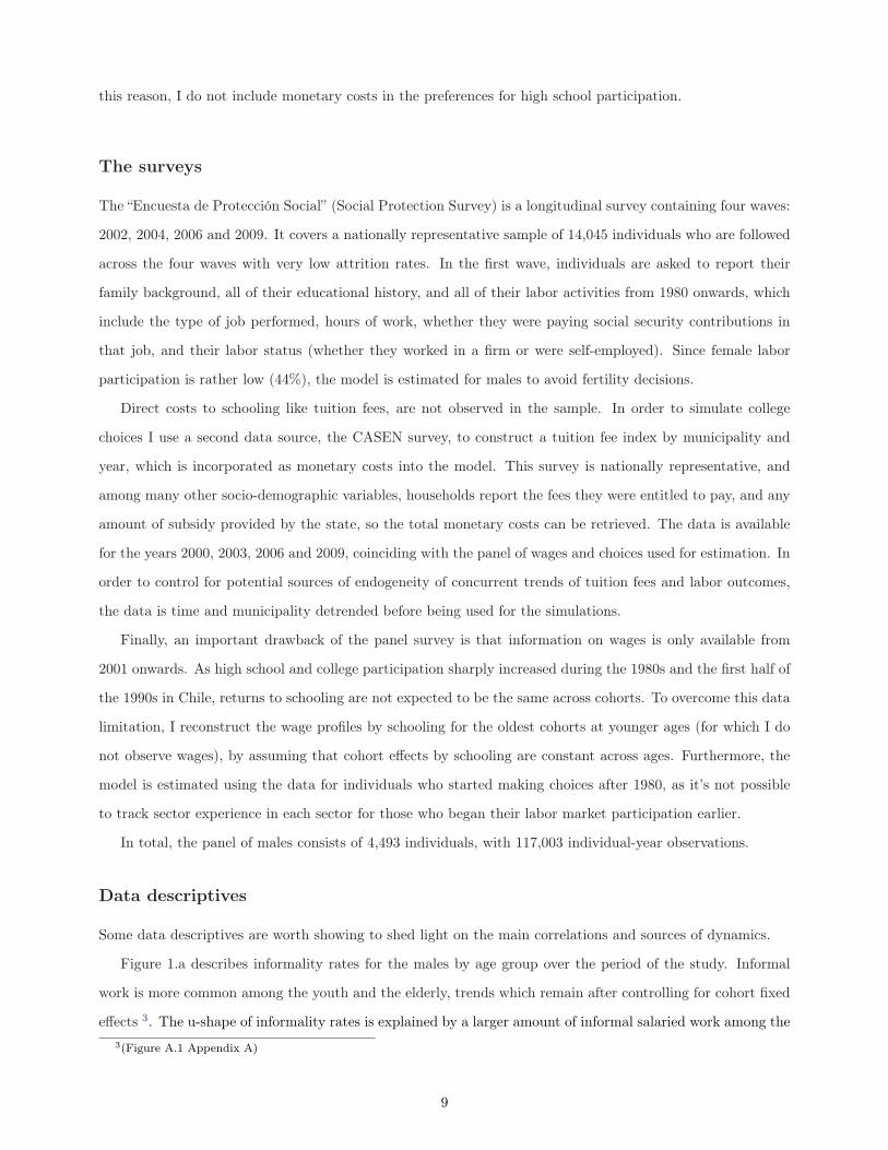
Figure 1.a describes informality rates for the males by age group over the period of the study. Informal

work is more common among the youth and the elderly, trends which remain after controlling for cohort fixed

effects 3. The u-shape of informality rates is explained by a larger amount of informal salaried work among the3(Figure A.1 Appendix A)

9

youth, and increasing participation in self-employment when workers become older. Consistent with evidence

from other Latin American countries, Figure 1.b also shows that informal labor participation decreases for

more educated workers, a trend which remains relatively stable over the life-cycle. These trends are similar

for women4. Remarkably, the strongest differences in informality arise between high school degrees and lower

than high school levels. Schooling differentials remain when the informality rates are analyzed separately for

the self-employed and salaried employees. 5.

Figure 1: a) Overall Informality Rates; b) Informality rates by schooling

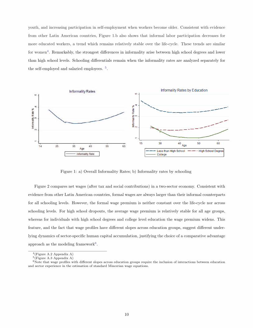
Figure 2 compares net wages (after tax and social contributions) in a two-sector economy. Consistent with

evidence from other Latin American countries, formal wages are always larger than their informal counterparts

for all schooling levels. However, the formal wage premium is neither constant over the life-cycle nor across

schooling levels. For high school dropouts, the average wage premium is relatively stable for all age groups,

whereas for individuals with high school degrees and college level education the wage premium widens. This

feature, and the fact that wage profiles have different slopes across education groups, suggest different under-

lying dynamics of sector-specific human capital accumulation, justifying the choice of a comparative advantage

approach as the modeling framework6.

4(Figure A.2 Appendix A)5(Figure A.3 Appendix A)6Note that wage profiles with different slopes across education groups require the inclusion of interactions between education

and sector experience in the estimation of standard Mincerian wage equations.

10

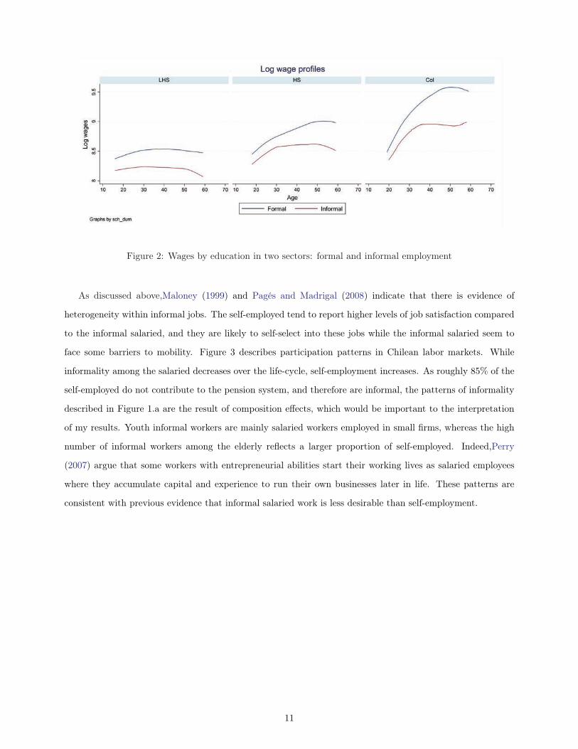
Figure 2: Wages by education in two sectors: formal and informal employment

As discussed above,Maloney (1999) and Pagés and Madrigal (2008) indicate that there is evidence of

heterogeneity within informal jobs. The self-employed tend to report higher levels of job satisfaction compared

to the informal salaried, and they are likely to self-select into these jobs while the informal salaried seem to

face some barriers to mobility. Figure 3 describes participation patterns in Chilean labor markets. While

informality among the salaried decreases over the life-cycle, self-employment increases. As roughly 85% of the

self-employed do not contribute to the pension system, and therefore are informal, the patterns of informality

described in Figure 1.a are the result of composition effects, which would be important to the interpretation

of my results. Youth informal workers are mainly salaried workers employed in small firms, whereas the high

number of informal workers among the elderly reflects a larger proportion of self-employed. Indeed,Perry

(2007) argue that some workers with entrepreneurial abilities start their working lives as salaried employees

where they accumulate capital and experience to run their own businesses later in life. These patterns are

consistent with previous evidence that informal salaried work is less desirable than self-employment.

11

Schooling Level Experience asformal and informal

Experience asself-employed andsalaried employee

LHS 69% 70%

HS 52% 32%

Col 40% 13%

Table 1: Fraction of workers with experience as formal/informal, and self-employed/salaried employees

Figure 3: Participation rates

Table 1 indicates that the probability of having some level of experience as informal or as a self-employed

in the sample is rather large, so there is mobility across sectors. The fraction of workers with experience as

both formal and informal, and as self-employed workers, decreases with schooling, which is consistent with

the data for other Latin American countries reported by Perry (2007). One the one hand, 69% of high school

dropouts have labor experience both in the formal and in the informal sectors, while these rates are lower for

individuals with high school degree and college level (52% and 40%). On the other hand, 70% of high school

dropouts have experience as salaried employees and of being self-employed, while these rates also decrease for

individuals with high school degree and college level (32% and 13%).

However, once workers enter a sector, the probability of switching to another sector is rather low, or

persistency in choices is large. For example, among the formal salaried workers, the probability of remaining

12

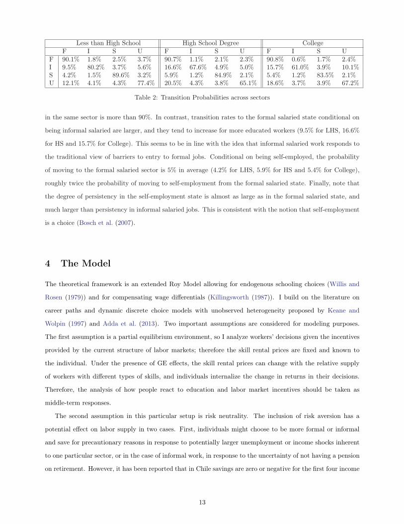
Less than High School High School Degree CollegeF I S U F I S U F I S U

F 90.1% 1.8% 2.5% 3.7% 90.7% 1.1% 2.1% 2.3% 90.8% 0.6% 1.7% 2.4%I 9.5% 80.2% 3.7% 5.6% 16.6% 67.6% 4.9% 5.0% 15.7% 61.0% 3.9% 10.1%S 4.2% 1.5% 89.6% 3.2% 5.9% 1.2% 84.9% 2.1% 5.4% 1.2% 83.5% 2.1%U 12.1% 4.1% 4.3% 77.4% 20.5% 4.3% 3.8% 65.1% 18.6% 3.7% 3.9% 67.2%

Table 2: Transition Probabilities across sectors

in the same sector is more than 90%. In contrast, transition rates to the formal salaried state conditional on

being informal salaried are larger, and they tend to increase for more educated workers (9.5% for LHS, 16.6%

for HS and 15.7% for College). This seems to be in line with the idea that informal salaried work responds to

the traditional view of barriers to entry to formal jobs. Conditional on being self-employed, the probability

of moving to the formal salaried sector is 5% in average (4.2% for LHS, 5.9% for HS and 5.4% for College),

roughly twice the probability of moving to self-employment from the formal salaried state. Finally, note that

the degree of persistency in the self-employment state is almost as large as in the formal salaried state, and

much larger than persistency in informal salaried jobs. This is consistent with the notion that self-employment

is a choice (Bosch et al. (2007).

4 The Model

The theoretical framework is an extended Roy Model allowing for endogenous schooling choices (Willis and

Rosen (1979)) and for compensating wage differentials (Killingsworth (1987)). I build on the literature on

career paths and dynamic discrete choice models with unobserved heterogeneity proposed by Keane and

Wolpin (1997) and Adda et al. (2013). Two important assumptions are considered for modeling purposes.

The first assumption is a partial equilibrium environment, so I analyze workers’ decisions given the incentives

provided by the current structure of labor markets; therefore the skill rental prices are fixed and known to

the individual. Under the presence of GE effects, the skill rental prices can change with the relative supply

of workers with different types of skills, and individuals internalize the change in returns in their decisions.

Therefore, the analysis of how people react to education and labor market incentives should be taken as

middle-term responses.

The second assumption in this particular setup is risk neutrality. The inclusion of risk aversion has a

potential effect on labor supply in two cases. First, individuals might choose to be more formal or informal

and save for precautionary reasons in response to potentially larger unemployment or income shocks inherent

to one particular sector, or in the case of informal work, in response to the uncertainty of not having a pension

on retirement. However, it has been reported that in Chile savings are zero or negative for the first four income

13

quantiles7. And second, risk averse workers might react to the incentives provided by the contributory pension

account, which are compulsory savings for formal workers. But as Attanasio et al. (2011) note, these incentives

are likely to affect labor supply decisions only for workers who are more than 45 years old, and they report that

for males in these age groups the effects are very low (less than 1.7% decrease in formal labor participation).

Nonetheless, an interesting extension of the model is the incorporation of risk averse individuals alongside both

private and pension savings to analyze how schooling and labor supply would change in response to credit

market imperfections.

In this modeling framework, workers then choose schooling and sector participation according to their com-

parative advantage, but transitions across sectors are costly, which might reflect the presence of labor market

rigidities. A worker’s comparative advantage is a complex vector, which includes observed and unobserved

skills, and tastes for non-wage job amenities. Unobserved skills are modeled as initial skill endowments by

including discrete and finite unobserved types in the fashion of Heckman and Singer (1984). Wage offers are

sector-specific and are the realization of a technology of skill production function that embodies the accumu-

lated human capital of an individual valued in a particular sector according to an equilibrium rental price.

The model attempts to reproduce the dynamics found in the data by explicitly incorporating labor market

expectations as part of the valuation of current choices. In the context of a human capital investment model,

this means two things. First, past schooling and labor choices determine the accumulated level of skills, which

could be rewarded differently in each sector depending on market prices. And second, individuals don’t know

for sure the future benefits of a particular choice in the present, but they know the distribution of shocks, so

they can evaluate the future expected rewards for every possible current choice.

It is worth stressing some model mechanisms. First, wage returns are heterogeneous. Therefore, the fact

that formal wages are larger on average doesn’t mean that this is true for everyone. Furthermore, conditional

on schooling and sector-experience some individuals might earn more in informal salaried jobs or in self-

employment if their initial skill endowments are better rewarded in these sectors, which reflects the fact

that skill endowments are not necessarily equally productive across sectors. Second, initial skill endowments

explicitly relate to schooling choices and productivity across sectors, as skill endowments act as a proxy for the

underlying ability of the individual, which might determine self-selection into higher levels of schooling. Third,

even if the accumulated human capital of an individual is better rewarded in a particular sector, she might end

up choosing another sector for several reasons. For example, she might value the non-wage attributes of the job

more, like the level of flexibility or autonomy, or she might face large search or psychological costs to transition

to the sector with a larger wage. Finally, these features have important implications for understanding how

people would react to incentives. For example, the effects of individual behavior of a decrease in income taxes

in the formal sector are reduced if non-monetary incentives are too important or if schooling attainment or7Butelmann and Gallego (2000). “Household Saving in Chile: Microeconomic Evidence”. Central Bank of Chile.

14

the choice of a sector are highly dependent on ability.

The timing of the model is as follows. Individuals make their first choice at age 14. They can achieve

three education levels: “Less than High School”, “High School Degree” or “College”. Everyone starts with

primary schooling which is completed at t = 0 (age 14). In the sample 96% of students complete this level. At

every subsequent period people decide whether to continue to the next schooling level, start working in formal

or informal jobs, or stay out of the labor market in unemployment or home production activities. Denote

m = {F, I} one of the three working sector choices, where F =formal salaried and I =informal salaried. The

choice of home production, non-participation or unemployment is denoted by U .

4.1 The State Space

Denote the state space Ω as the set of variables that define the state-dependency of individual utilities over

time. I estimate a life-cycle model so the time dimension t is the age of the individual. I detrend the data

on wages and tuition fees to control for macroeconomic trends, and I take out cohort effects to compute data

moments. Edit is the schooling level of individual i at age t. Then Edit = {LHS,HS,Col} or Less than High

School, High School Degree level, and College level. Accordingly, labor experience accumulates by sector.

Finally, I denote the unobserved ability by μi. Higher ability individuals self-select more into schooling,

and at the same time, people have different sets of skills that make them more productive in one sector than in

another, driving their choices. For example, entrepreneurial ability might drive self-selection into informal jobs

or self-employment, while the ability to work in structured work environments might drive self-selection into

formal jobs. Both of these are known by the individual and fixed from age 14, or t = 0. On the other hand,

they are unobserved by the econometrician and need to be estimated along with the rest of the parameters.

I incorporate permanent unobserved heterogeneity by modeling a discrete number k of unobserved types

(Heckman and Singer (1984)), so that μk is an indicator variable for type k. The use of a discrete and finite

number of types is important to make the dynamic programming problem tractable.

4.2 Flow Utilities

At every period, individuals derive an instantaneous utility from attending school, staying at home or working

in an economic sector. The costs of that decision are, in the case of schooling, foregone expected earnings

or rewards from leisure/home production. When choosing the working sector, I also allow for non-monetary

rewards coming from sector-specific job attributes.

Denote the vector of available choices at t by {Ed,m,U}. Since everyone at t = 0 starts with Edit = LHS,

people can make further schooling choices only for High school degree or College, thenEd = {HS,Col}. Denote

UEdit the instantaneous utility of attending schooling at level Ed. Then,

15

UEdk,R = γEd

1,kμk − TCEdR − ηEd

where TCEdiR is the tuition fee index constructed from household data, which varies by schooling level Ed

and municipality R. The index is constructed with detrended costs varying over time and across municipalities

in order to control for potential concurrent trends with wages and choices. The factor load γEd1,k represents

psychic costs or the consumption value of the schooling decision, which may capture both heterogeneous

abilities and family background which translates into financial constraints to attending high school or college.

The term ηEdt is a preference shock to schooling including the non-monetary costs of school attendance not

observed in the data.

The utility of working in sector m is

Umt,k = γm

2,Ed Wmt,k

− γm3,Ed + γm

4 t+ γm5 t2

where Wmtk is the gross wage offer the individual type k observes at age t in sector m and dit is the choice

the individual makes at age t.8Several additional terms affect sector preferences: γm2,Ed is the wage valuation,

which emphasizes both the marginal utility of income and the valuation of some sector amenities that are

non-separable in the utility function. Additional sources of heterogeneity are included in this parameter by

allowing it to vary across different sectors and education levels. γm3,Ed captures the worker’s valuation of non-

wage sector amenities which are separable in the utility function. One can interpret this parameter as fixed

costs of working, which are also allowed to vary by education levels. This parameter is relevant to understand

by how much individuals compensate wage differentials with non-wage sector attributes. A quadratic function

in age is also incorporated to capture the fact that individuals at different ages might have different tastes for

insurance and/or labor market participation in one particular sector. The parameter capturing age effects is

γm4 and γm

5 .

The utility of unemployment/leisure/home production is

UUt,k = γU

1,kμk − ηUt

8In a model with risk neutral individuals and returns from the stock markets similar to the interest rate, the timing doesnot matter when social security contributions such as pension retirement are taken into account. To the extent that there is fullcapitalization, as in the Chilean case, I consider gross wages, which in the formal sector already account for the total compensationincluding social security contributions.

16

The reward that individual type k obtains from staying at home depends on unobserved skills captured by

γU1k, and preference shocks ηUt , which is a random component reflecting uncertainty in the valuation of leisure

or home production. For example, pregnancy can increase the valuation of unemployment for women.

Finally, the model also explicitly includes transition costs, which are explained below in the section on

value functions. These costs are required to be included in order to match the high levels of persistence found

in the data.

4.3 The Wage Offer

Every time individuals choose to study they forego earnings from work. Since we have different working sectors,

every time individuals choose a sector they also forego earnings in another sector. Wages are a function of

the skill production function Hmt,k and skill rental prices rmt . As it was specified above, skill functions vary by

sector reflect the existence of different production functions across the formal and the informal sector, which

might translate into different marginal productivities of each skill component. The human capital accumulated

by workers is a function of their schooling level, their accumulated sector experience in the same sector and

across sectors, sector-specific unobserved abilities, and productivity shocks.

Wmt,k = rmt Hm

t,k = rmt f(Ed,XF , XI , μk, εmt )

Given a functional form for the skill function (exponential in this case), the sector-specific log wage offer

can be defined as follows,

lnWmt,k = αm

0,kμk + αm1 HS + αm

2 Col + αm3,Edln(1 +XF

t ) + αm4,Edln(1 +XI

t ) + εmt

where αm0k represents the rental price for the initial endowment in sector m for individual type k, and

captures selection across choices. αm1 and αm

2 capture the average returns to schooling levels. Since the data

wage profiles by sector and education show very different slopes, which also vary along the life-cycle, I estimate

returns to experience varying by education level, captured by the parameters αm3,Ed and αm

4,Ed.

Finally, in order to persistency in wages from unobserved factors, I include persistent productivity shocks

whose sector-specific innovations are allowed to be correlated across sectors

εmt = ρmεmt−1 + ξmt

ξmt ∼ N(0,Σ)

17

4.4 Uncertainty

The source of uncertainty in the model comes from preference and productivity shocks. Preference shocks

are modeled following an extreme value type 1 distribution, while innovations in persistent wage shocks are

normally distributed. Shocks are important to produce mobility across all choices in t because they shape

expected utilities in each of the alternative choices from t+ 1 to T , affecting rewards from current choices. It

is likely that innovations of productivity shocks are correlated across choices; that is why I draw wage shocks

from a multivariate normal distribution. Sector-specific autocorrelations and the distribution of innovations

are identified by the time series properties of wage data, so these parameters are estimated along the rest of

structural parameters.

4.5 Recursive problem

Self-selection into schooling and jobs is based on expected earnings, which depend on current choices. This

entails non-separability over time. The model dynamics are as follows: all individuals start at age 14 having

finished primary school. This is a fairly safe assumption as 96% of the sample actually did finish primary

schooling (in Chile primary school has effectively been compulsory since 1962). Every year they must choose

whether to continue studying for an extra year of secondary schooling, dropout and start working or, stay out

of the labor force. At age 18 they must decide whether to continue to College level or drop out of education.

If they drop out of school before the 4th level of high school then their education level stays at Edt = LHS

(Less than High School). If they dropout straight after the 4th level of secondary school then Edt = HS (High

School degree), and if they continue studying to College level then Edt = Col (College). The maximum level

of schooling is standardized to 5 years of College. If an individual drops out at any schooling level, she cannot

go back to school, a fact that is supported by the data.

If an individual decides to switch sector, she pays a fixed cost ci,j to move from sector i in t − 1 to j in

t. The purpose of these costs is to capture high levels of choice persistence in the data, which can be driven

by several factors like search costs, skill depreciation or psychological costs of transitions. They might also

capture certain labor rigidities that could partially explain mobility rates.

Denote by Ωt = {Edt, XF , XI , μk, R, εmt } the state space of type k at age t. Then the value of education

at level Ed = {HS,Col} is

V Edt,k (Ωt) = UEd

t,k + βEmax{

V Edt+1,k(Ωt+1), V m

t+1,k(Ωt+1)− cEd,m, V Ut+1,k(Ωt+1)

}

By choosing schooling individuals obtain the instantaneous utility UEdit plus the discounted expected max-

imum value over the available alternatives at t+1: continuing to the following schooling level, working in one

of the two sectors m = {F, I}, or staying out of the labor market. Expectations are taken over the distri-

18

bution of preference and productivity shocks implied by choices. Notice that Xit+1 = Xit when individuals

choose schooling and that they pay a transition cost only when moving to work, but not when moving to

unemployment/leisure/home production.

Similarly, the value of working as a formal-employee at t is,

V mt,k(Ωt) = Um

t,k + βEmax{

V mt+1,k(Ωt+1), V m′

t+1,k(Ωt+1)− cm,m′, V U

t+1,k(Ωt+1)

}

where it is clear that the worker cannot go back to school, and if she wants to switch sector, she has to

pay a transition cost cm,m′. By choosing sector m, individuals accumulate another year of experience in that

sector, which translates into an increase in the valuation of all choices rewarding labor experience in sector m

at age t+ 1.Finally, the value of unemployment/leisure/home production is

V Ut,k(Ωt) = UU

t,k + βEmax{

V mt+1,k(Ωt+1)− cU,m, V m′

t+1,k(Ωt+1)− cU,m′, V U

t+1,k(Ωt+1)

}

where the choice of unemployment does not alter the state space for the next period.

4.6 Mobility

In the model, mobility across sectors is generated by three sources. First, an individual may switch to another

sector if there is a large positive shock in the sector she intends to move to, and the gains in productivity due

to this shock and to the returns to skills in the new sector are larger than the mobility costs and the potential

losses in the returns to skills if she stays. Second, even if the shocks and transition costs across sectors are

exactly the same, the worker might still want to switch if an additional year of experience in the new sector is

better rewarded than an additional year of experience in the current sector. Note that experience accumulated

in each sector is potentially rewarded in all sectors with different rental prices. Finally, mobility costs across

sectors might prevent individuals from switching. For example, if at some point in the life-cycle a low-skilled

informal worker faces a negative shock, she might consider switching to a similar formal job as her experience

would also be rewarded in the new job. However, this decision might be prevented by unaffordable entry costs,

search costs, rationing, or the lack of networks, preventing movement.

19

5 Model Solution and Estimation

5.1 Solution Method

Dynamic discrete choice models do not have an analytical solution. Within a finite horizon context, the model

must be solved numerically using backward recursion methods. At period T , each individual draws random

shocks from the multidimensional error vector (ηT , εT ) and chooses the alternative that yields the maximum

instantaneous utility evaluated at every possible state space combination of schooling and labor histories. I

assume that the terminal value function over the life-cycle is VT+1 = 0. I denote d∗t = {Ed,m,U} the optimal

choice at every period. Then, at period T individuals solve

d∗T = argmax(UEdT , Um

T , UUT )

At period every period t, two steps are required to compute the value functions. First, they need to evaluate

expectations over t+1 computing the Emax functions, where expectations are taken over (ηt+1, εt+1), evaluated

at every possible choice and state space combination at t.

To solve for the fact that wage shocks in t+1 depend on the realizations of wage shocks in t, I follow Galindev

and Lkhagvasuren (2010) to approximate persistent shocks in more than one dimension with innovations which

are potentially correlated across dimensions. They adapt Tauchen’s method (Tauchen (1986)) by using Markov

Chain processes, which they prove is an efficient method provided that the autocorrelation parameters are

not close to unit root9. The evaluation of the Emax function then involves a multidimensional numerical

integration as follows,

Emax[V Edt , V m

t , V UTt] =

ˆ

εt

⎧⎨⎩ˆ

ηt

max[V Edt , V m

t , V Ut /d∗t−1,Ωt−1, εt−1]f(η)dη

⎫⎬⎭ f(εt | εt−1)dε

Where f(εt | εt−1) is the transition matrix for the Markov process of wage shocks. This matrix is a function

of the autocorrelation parameters ρm and the variance of wage innovations Σ. The advantage of modeling

preference shocks ηit with an extreme value Type I distribution is that the expected value (Emax) has a

closed form expression so we can decrease the dimensions of numerical integration. Therefore, the evaluation

of the Emax function only involves the numerical integration across the dimensions of wage shocks, which are

normally distributed.

Second, I evaluate the instantaneous utilities at t−1, again for every possible combination of the steady state9The analysis of the time series of the wage residuals show that the autocorrelation parameters in both sectors are close to 0.9

20

at that period, drawing the error vectors (ηt−1, ξt−1) and compute the value functions at t−1: (V Edt−1, V

mt−1, V

Ut−1).

The optimal choice at t− 1 is then obtained from

d∗t−1 = argmax(V Edt−1, V

mt−1, V

Ut−1)

The process is then repeated in the same fashion until t = 0, where the outcome is the evaluation of the

optimal choice d∗t for every combination of the state space Ωt in every period.

5.2 Model Identification

Three aspects of model specification are worth discussing in my modeling framework. First, the model does not

suffer from an initial condition problem. As Aguirregabiria and Mira (2010) note, in a model with unobserved

heterogeneity, if the initial state space varies across individuals in the sample, one needs to fully specify how the

distribution of unobserved heterogeneity changes with initial states. Initial endowments in the first period of

the model are likely to be correlated with observable states. Therefore, if there is variation in the distribution

of initial states in the sample, one would need to use some parametric or non-parametric specification of how

individuals made choices in the past conditional on unobservables, and solve it backwards until the state

space becomes independent of permanent unobserved heterogeneity. In this particular case, almost everyone

in the sample finished primary school (primary schooling has been compulsory in Chile since 1962), and thus

everybody started with the same education and experience.

To identify wage returns in different sectors, I exploit a large sample variation of wages by sector, schooling,

and sector experience, to estimate counterfactual wage returns. I observe data for individuals from different

cohorts, so I also exploit time variation to reconstruct wage and participation moments by age. I control for

cohort effects in sector wages to incorporate the potential variation in returns over time as a result of merging

data from different cohorts. With regard to the identification of unobserved heterogeneity parameters varying

by type, I attempt to identify the whole distribution of wage profiles by matching different percentiles of sector

wage distributions by schooling.

In order to identify the preference parameters in non-working activities, Todd and Wolpin (2010) note

that one only needs to specify an exclusion restriction in the working alternatives. In this case, observable

education, sector experience, and accepted wages are sufficient statistics to identify those parameters. The

identification of preference parameters in the working alternatives require further exclusion restrictions in the

non-working alternatives. I exploit the variability on tuition costs of schooling across municipalities and years

for this purpose. The CASEN survey is a nationally representative household survey which reports the tuition

costs actually paid by families at high school and college levels and any amount of subsidies received, for each

21

of the years 1998, 2000, 2003, 2006 and 2009. I use this data to retrieve the total tuition fees the family would

have to pay at each education level, and I construct a tuition cost index by municipality and year at each level

of education, which is incorporated as a proxy for the monetary costs in the model simulations. I take out

time and municipality dummies from the construct in order to control for concurrent trends with wages and

labor supply.

TCEdt,R = δEd

0 + δEd1 ∗REd + δEd

2 ∗ t+ νEdt,R

so the average residual by time is then used to simulate schooling choices

UEdk,R = γEd

1,kμk − νEdR − ηEd

Finally, in order to identify transition costs across sectors, I exploit the variation of mobility rates by

schooling that I observe in the data.

5.3 Estimation

I estimate the model by Indirect Inference (Gourieroux et al. (1993)). Meghir and Rivkin (2010) emphasize the

use of simulation methods for structural estimation, as they do not use all of the information and restrictions

implied by the model, given the available data, as MLE methods do, thus speeding up the estimation process.

The accuracy of the estimated parameters depends only on good specification of the data identifying moments,

which is relatively simple in linear models.

The idea of indirect inference is to simulate data with the model at each iteration of the vector of structural

parameters (θ)10The process starts by simulating data from an initial vector of structural parameters (θ0), and

passing both the actual and simulated data by an auxiliary model, usually a system of linear regressions, to

generate a set of data auxiliary parameters β, and the analogous set of simulated auxiliary parameters β(θ).

At each iteration of the structural parametersθj , Indirect Inference optimally finds the estimates of θj+1that

minimize the distance between the data and simulated auxiliary parameters, until convergence is achieved.

For example, in the first iteration the set of initial simulated auxiliary estimates is β1(θ0) and the following

set of converging parameters θ1is found by minimizing a weighted distance between the simulated and data

auxiliary parameters. The objective function at given iteration j is given by the metric

Minθ(β − βj(θ))′W (β − βj(θ))

10Simulating moments involves a forward recursive data generation process which uses as inputs the initial guess of the parametervector (θ0) , a random draw of the vector of shocks for every individual at every age (ηi,t, εi,t) , and the optimal policy functiond∗t . The forward recursion process works as follows: in period t= 1 the optimal choice is retrieved by evaluating the policyfunction in Ω1 , whereas the simulated counterfactual wages are obtained by evaluating Wm(θ0, ε1,Ω1) . The optimal choiced∗1 involves individuals choosing either education, work in sector m or unemployment in the first period, so the state spaceis updated accordingly for the next period accumulating either education or sector experience, and Ω2 is evaluated for eachsimulated individual. This process is repeated until the whole sequence of choices d∗t = [d∗1, .....d

∗T ] and counterfactual wages

Wmt = [Wm

1 , .....WmT ] are obtained and used to simulate moments. I simulate data on choices and counterfactual wages for

N = 10, 000 individuals in T = 52 periods.

22

Given the large number of moments required to identify the model, I use the diagonal of the optimal weighting

function defined by W = diag(V CV (β)−1), which is obtained from the auxiliary estimates. The full optimal

weigting function is used in a second stage to estimate efficient standar errors.

A standard selection problem involves the estimation of a set of auxiliary linear regressions including log

wage regressions and LPM models for participation both with the actual data and the simulations. Building

on this approach, I use the following auxiliary model

⎡⎢⎢⎢⎢⎢⎢⎢⎣

lnWit

P (dit = J)

P (dit = J |dit−1 = J ′)

ΔlnWJJ′it

⎤⎥⎥⎥⎥⎥⎥⎥⎦

= Z′itδ + νit ∼ N(0,Λ)

which involves estimating a log wage regression, the probability of participation in sector J , the transition

probability from sector J ′ to sector J , and the growth of log wages across sectors, on a vector of observable

variables Zit which includes the schooling level, sector experience, age, and tuition costs. Additionally, we

must include in the set of moments the time series properties of the log wage regressions by sector, namely

the autocorrelation and the VCV matrix of the shocks innovations. The vector of auxiliary parameters β to

be matched are the coefficients of the auxiliary regressors (δ), and the VCV of the residuals Λ.

Asymptotic Properties

Standard errors of the estimates are obtained by applying the asymptotic properties of Indirect Inference

Estimators described in Gourieroux et al. (1993), under which

√NT (θ̂ − θo) −→ N(0, [d′W ∗d]−1)

where W ∗ is the optimal weigting matrix and where d = ∂β

∂θ̂is the score evaluated at the optimum.

However, in the the objective function above was minimized using W = diag(V CV (β)−1), which delivers

consistent but not efficient estimates. Efficient standard errors are then computed using a two-stage procedure.

The first stage consists in obtaining consistent estimates with the sub-optimal weigting matrix. In the second

stage, I use the model evaluated at the optimum to generate S simulated panels and their corresponding set

of moments, from where I can construct an estimate of V CV (β) and the optimal weighting matrix. I evaluate

the scores also by simulation methods. Each of the first-stage structural estimates are shocked in small values

(ε) one at a time, and I evaluate the partial derivatives for each of the moments ∂β

∂(θ̂+ε).

23

Smoothing the Objective Function

Using Indirect Inference in discrete choice models imposes important challenges. As Magnac et al. (1999)

note, in discrete choice environments, objective functions are step functions of the structural parameters,

which makes the use of derivative-based methods difficult. Derivative-based methods are generally preferred

to local or global search methods because of speed and accuracy considerations. I use the approach presented

by Keane and Smith (2003) who propose the use of a smoothing function allowing estimation by gradients.

To correct for the choppiness of the objective function, they propose an alternative system of auxiliary

regressions to be used in the simulated data, which consists in proxying dJit by a smooth function of the

structural parameters obtained from simulated value functions

gJ(θ) =exp

(V J(θ)/λ

)∑

j exp (VJ(θ)/λ)

where gJ(θ) can be interpreted as the asymptotic probability of choosing alternative J , andλis a calibrated

smoothing parameter. The mirroring system of auxiliary regressions then becomes

⎡⎢⎢⎢⎢⎢⎢⎢⎢⎣

∑J

gJt ∗ lnW Jit

gJt

gJJ′

t

gJJ′

t ∗ΔlnW JJ ′it

⎤⎥⎥⎥⎥⎥⎥⎥⎥⎦= Z ′

itδ(θ) + νit ∼ N(0,Λ)

Note that in the simulated auxiliary system we can observe each of the counter-factual wages.Therefore,

the simulated log wages are the expected log-wages across sectors.

Identifying Moments

In order to gain identifying power of the unobserved heterogeneity parameters, I add to the set of auxiliary

parameters the proportions of people below wage percentiles {1.0,25,50,75 and 90} by education level and

sector, and regressions of log wages by sector on education, experience and age (Blundell et al. (2013)). The

set of moments involves 155 auxiliary parameters used to estimate 45 structural parameters.

Table 3 describes the set of matching moments linked to the set of structural parameters I attempt to

identify.

Finally, besides the discussion on the model identification, I check empirically whether the set of moments

proposed actually identifies the set of structural parameters. I perform Montecarlo simulations using the model

24

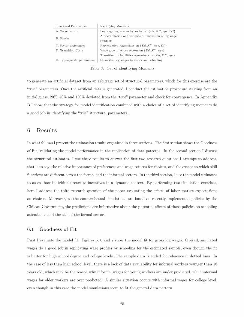
Structural Parameters Identifying Moments

A. Wage returns Log wage regressions by sector on {Ed,Xm, age, TC}

B. ShocksAutocorrelation and variance of innovation of log wage

residuals

C. Sector preferences Participation regressions on {Ed,Xm, age, TC}D. Transition Costs Wage growth across sectors on {Ed,Xm, age}

Transition probabilities regressions on {Ed,Xm, age}E. Type-specific parameters Quantiles Log wages by sector and schooling

Table 3: Set of identifying Moments

to generate an artificial dataset from an arbitrary set of structural parameters, which for this exercise are the

“true” parameters. Once the artificial data is generated, I conduct the estimation procedure starting from an

initial guess, 20%, 40% and 100% deviated from the “true” parameter and check for convergence. In Appendix

B I show that the strategy for model identification combined with a choice of a set of identifying moments do

a good job in identifying the “true” structural parameters.

6 Results

In what follows I present the estimation results organized in three sections. The first section shows the Goodness

of Fit, validating the model performance in the replication of data patterns. In the second section I discuss

the structural estimates. I use these results to answer the first two research questions I attempt to address,

that is to say, the relative importance of preferences and wage returns for choices, and the extent to which skill

functions are different across the formal and the informal sectors. In the third section, I use the model estimates

to assess how individuals react to incentives in a dynamic context. By performing two simulation exercises,

here I address the third research question of the paper evaluating the effects of labor market expectations

on choices. Moreover, as the counterfactual simulations are based on recently implemented policies by the

Chilean Government, the predictions are informative about the potential effects of those policies on schooling

attendance and the size of the formal sector.

6.1 Goodness of Fit

First I evaluate the model fit. Figures 5, 6 and 7 show the model fit for gross log wages. Overall, simulated

wages do a good job in replicating wage profiles by schooling for the estimated sample, even though the fit

is better for high school degree and college levels. The sample data is added for reference in dotted lines. In

the case of less than high school level, there is a lack of data availability for informal workers younger than 18

years old, which may be the reason why informal wages for young workers are under predicted, while informal

wages for older workers are over predicted. A similar situation occurs with informal wages for college level,

even though in this case the model simulations seem to fit the general data pattern.

25

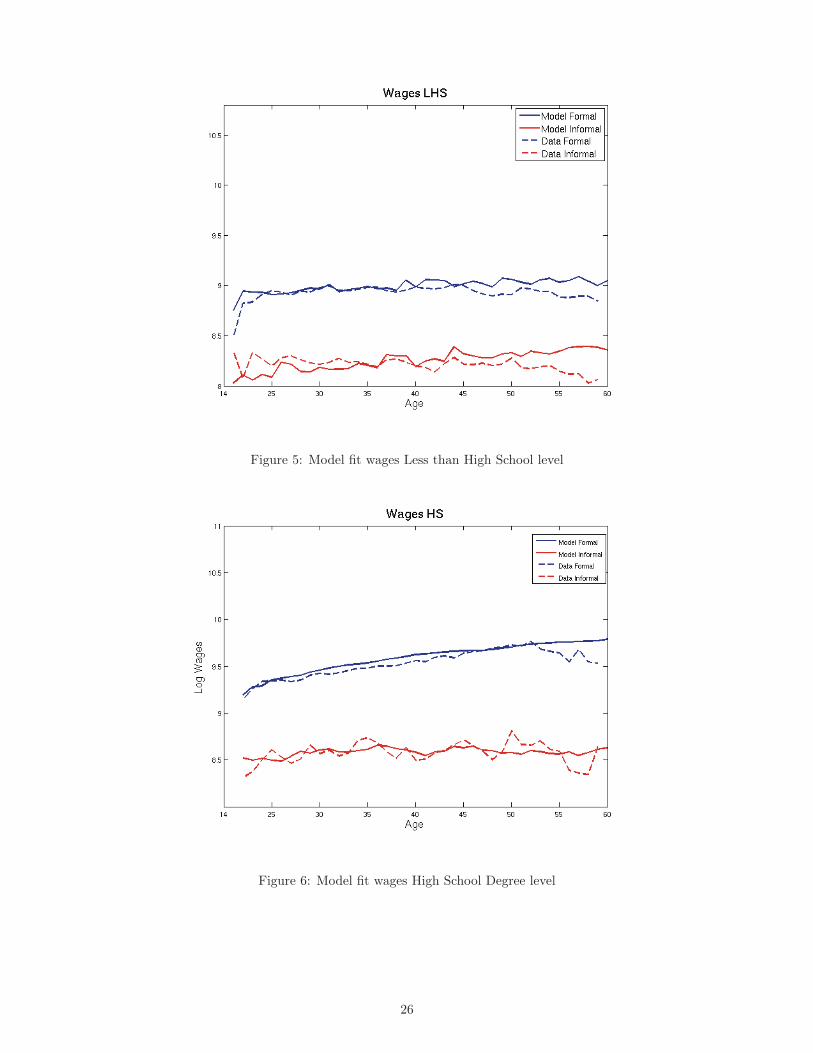
Figure 5: Model fit wages Less than High School level

Figure 6: Model fit wages High School Degree level

26

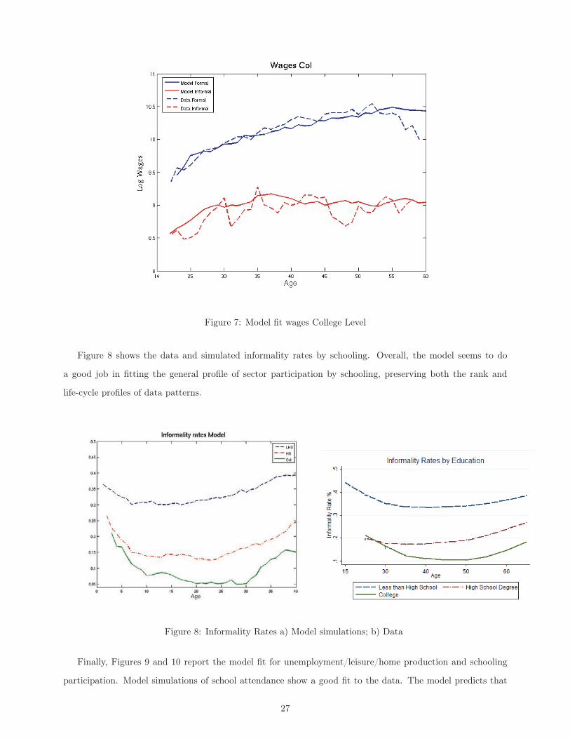
Figure 7: Model fit wages College Level

Figure 8 shows the data and simulated informality rates by schooling. Overall, the model seems to do

a good job in fitting the general profile of sector participation by schooling, preserving both the rank and

life-cycle profiles of data patterns.

Figure 8: Informality Rates a) Model simulations; b) Data

Finally, Figures 9 and 10 report the model fit for unemployment/leisure/home production and schooling

participation. Model simulations of school attendance show a good fit to the data. The model predicts that

27

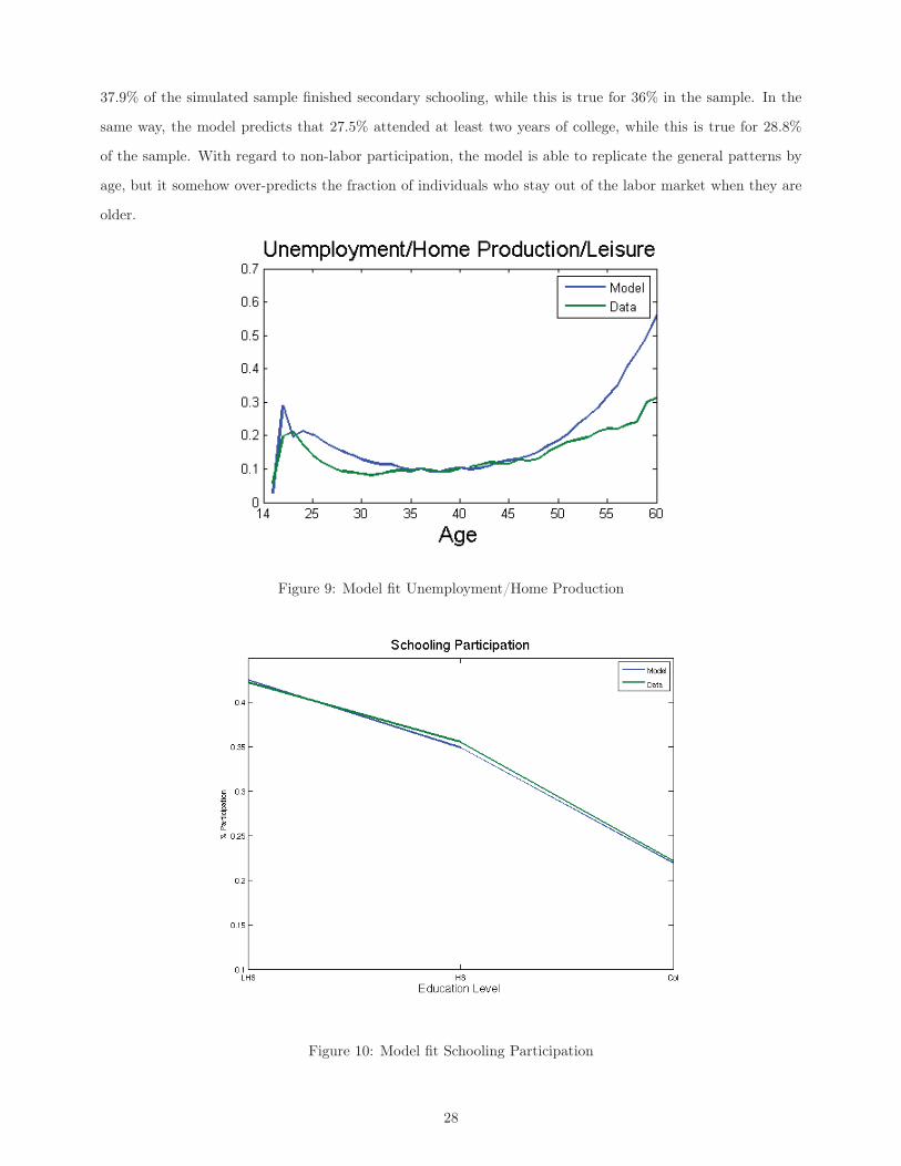
37.9% of the simulated sample finished secondary schooling, while this is true for 36% in the sample. In the

same way, the model predicts that 27.5% attended at least two years of college, while this is true for 28.8%

of the sample. With regard to non-labor participation, the model is able to replicate the general patterns by

age, but it somehow over-predicts the fraction of individuals who stay out of the labor market when they are

older.

Figure 9: Model fit Unemployment/Home Production

Figure 10: Model fit Schooling Participation

28

6.2 Structural Estimates

Table 4 shows the estimated preference parameters, which shed light about the relative importance of wage

returns and preferences for sector amenities, and the estimated transition costs.

First, I assess the relative importance between wage returns and sector preferences by comparing wage

valuations and fixed cost of working. Marginal valuation of incomes are statistically larger than fixed cost of

work for individuals with Less than High School and High School degree, while they are similar for individuals

with College level. Therefore, less educated people seem to be more liquidity-constrained, as their valuation

for the cash-in-hand aspects of the job are more important. The trends go in opposite directions looking at

fixed costs to work. Individuals at higher levels of education seem to value more the non-monetary aspects of

the wage, no matter the sector in which they participate.

Second, the comparisons of these two parameters across sectors within education level brings important

considerations. For Less than High School individuals, fixed costs to work are fairly similar across sectors,

while they tend to value wage returns in informal activities more. These findings are consistent with pre-

vious evidence that low-educated informal workers tend to value the possibility of evading taxes and social

security contributions from which they derive little value, and with evidence that this education group not

only participates more of informal activities, but mobility rates between formal and informal activities are

larger (Maloney (2004), Pagés and Stampini (2007)). Moreover, while marginal valuation of income is similar

across sectors for individuals with High School degree and College level, fixed costs of work are consistently

larger in the informal sector for these education groups. In summary, more educated workers face net costs in

the informal sector, so the participation of these workers in informal activities should be explained by other

reasons like returns to skills.

Third, predicted transition costs are larger for transitions towards the formal sector either from informal

jobs or from non-participation. As these mobility costs have been estimated taking into account comparative

advantage factors, preferences and shocks, I interpret these findings as evidence of the presence of some barriers

to mobility to the formal sector.11

11Note that estimated switching costs are very large in all directions. Kennan (2008) argues that when there are few transitionsin the data, estimated switching costs are implausibly large, because transitions must be attributed to unobserved payoff shocks.Therefore, he notes that observed switches must be attributed to unobserved payoff shocks and in order to evaluate their magnitude,one should evaluate how large the switching costs are conditional on the switch being made. When shocks are drawn from thetype I extreme value distribution, he shows that the average transition costs of moving from sector i to j are the estimated costsnet of the difference in payoff shocks,

AV Costij = TRij − E[ηjt − ηit | djt = 1]

As a result, the monetary magnitude of the estimated transition costs is much smaller once they are adjusted by shocks.

29

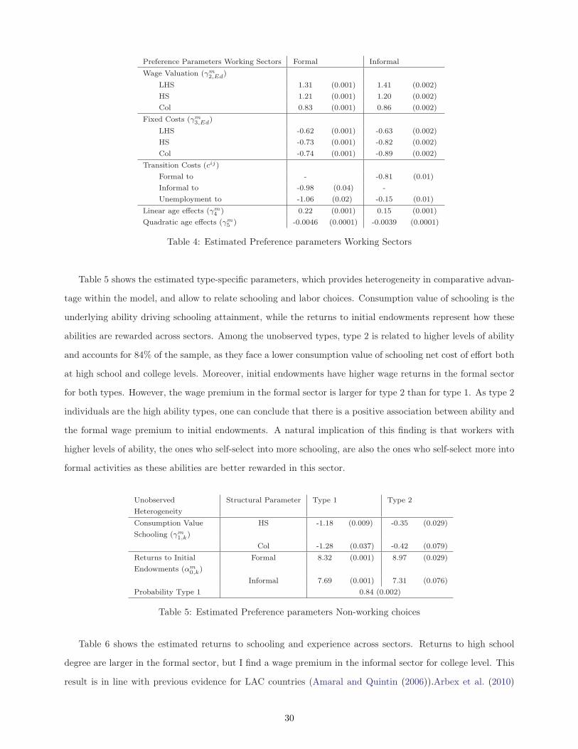
Preference Parameters Working Sectors Formal InformalWage Valuation (γm

2,Ed)LHS 1.31 (0.001) 1.41 (0.002)HS 1.21 (0.001) 1.20 (0.002)Col 0.83 (0.001) 0.86 (0.002)

Fixed Costs (γm3,Ed)

LHS -0.62 (0.001) -0.63 (0.002)HS -0.73 (0.001) -0.82 (0.002)Col -0.74 (0.001) -0.89 (0.002)

Transition Costs (cij)

Formal to - -0.81 (0.01)Informal to -0.98 (0.04) -Unemployment to -1.06 (0.02) -0.15 (0.01)

Linear age effects (γm4 ) 0.22 (0.001) 0.15 (0.001)

Quadratic age effects (γm5 ) -0.0046 (0.0001) -0.0039 (0.0001)

Table 4: Estimated Preference parameters Working Sectors

Table 5 shows the estimated type-specific parameters, which provides heterogeneity in comparative advan-

tage within the model, and allow to relate schooling and labor choices. Consumption value of schooling is the

underlying ability driving schooling attainment, while the returns to initial endowments represent how these

abilities are rewarded across sectors. Among the unobserved types, type 2 is related to higher levels of ability

and accounts for 84% of the sample, as they face a lower consumption value of schooling net cost of effort both

at high school and college levels. Moreover, initial endowments have higher wage returns in the formal sector

for both types. However, the wage premium in the formal sector is larger for type 2 than for type 1. As type 2

individuals are the high ability types, one can conclude that there is a positive association between ability and

the formal wage premium to initial endowments. A natural implication of this finding is that workers with

higher levels of ability, the ones who self-select into more schooling, are also the ones who self-select more into

formal activities as these abilities are better rewarded in this sector.

UnobservedHeterogeneity

Structural Parameter Type 1 Type 2

Consumption ValueSchooling (γm

1,k)HS -1.18 (0.009) -0.35 (0.029)

Col -1.28 (0.037) -0.42 (0.079)Returns to InitialEndowments (αm

0,k)Formal 8.32 (0.001) 8.97 (0.029)

Informal 7.69 (0.001) 7.31 (0.076)Probability Type 1 0.84 (0.002)

Table 5: Estimated Preference parameters Non-working choices

Table 6 shows the estimated returns to schooling and experience across sectors. Returns to high school

degree are larger in the formal sector, but I find a wage premium in the informal sector for college level. This

result is in line with previous evidence for LAC countries (Amaral and Quintin (2006)).Arbex et al. (2010)

30

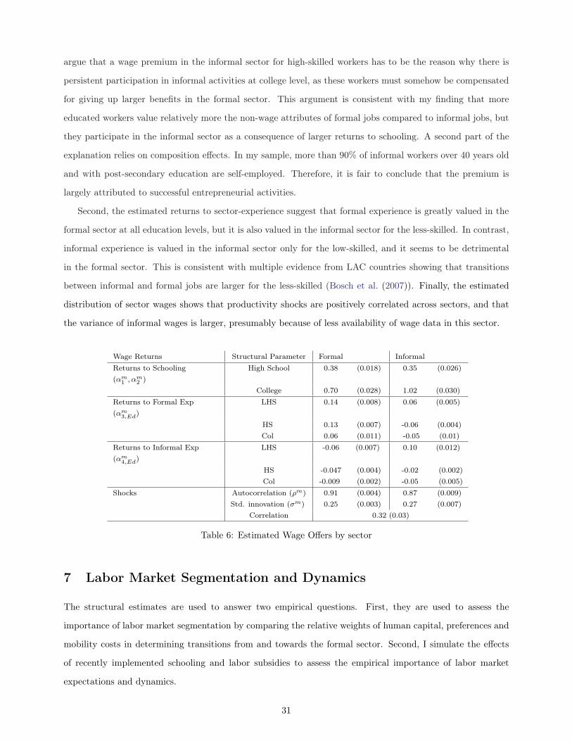
argue that a wage premium in the informal sector for high-skilled workers has to be the reason why there is

persistent participation in informal activities at college level, as these workers must somehow be compensated

for giving up larger benefits in the formal sector. This argument is consistent with my finding that more

educated workers value relatively more the non-wage attributes of formal jobs compared to informal jobs, but

they participate in the informal sector as a consequence of larger returns to schooling. A second part of the

explanation relies on composition effects. In my sample, more than 90% of informal workers over 40 years old

and with post-secondary education are self-employed. Therefore, it is fair to conclude that the premium is

largely attributed to successful entrepreneurial activities.

Second, the estimated returns to sector-experience suggest that formal experience is greatly valued in the

formal sector at all education levels, but it is also valued in the informal sector for the less-skilled. In contrast,

informal experience is valued in the informal sector only for the low-skilled, and it seems to be detrimental

in the formal sector. This is consistent with multiple evidence from LAC countries showing that transitions

between informal and formal jobs are larger for the less-skilled (Bosch et al. (2007)). Finally, the estimated

distribution of sector wages shows that productivity shocks are positively correlated across sectors, and that

the variance of informal wages is larger, presumably because of less availability of wage data in this sector.

Wage Returns Structural Parameter Formal InformalReturns to Schooling(αm

1 , αm2 )

High School 0.38 (0.018) 0.35 (0.026)

College 0.70 (0.028) 1.02 (0.030)Returns to Formal Exp(αm

3,Ed)LHS 0.14 (0.008) 0.06 (0.005)

HS 0.13 (0.007) -0.06 (0.004)Col 0.06 (0.011) -0.05 (0.01)

Returns to Informal Exp(αm

4,Ed)LHS -0.06 (0.007) 0.10 (0.012)

HS -0.047 (0.004) -0.02 (0.002)Col -0.009 (0.002) -0.05 (0.005)

Shocks Autocorrelation (ρm) 0.91 (0.004) 0.87 (0.009)Std. innovation (σm) 0.25 (0.003) 0.27 (0.007)

Correlation 0.32 (0.03)

Table 6: Estimated Wage Offers by sector

7 Labor Market Segmentation and Dynamics

The structural estimates are used to answer two empirical questions. First, they are used to assess the

importance of labor market segmentation by comparing the relative weights of human capital, preferences and

mobility costs in determining transitions from and towards the formal sector. Second, I simulate the effects

of recently implemented schooling and labor subsidies to assess the empirical importance of labor market

expectations and dynamics.

31

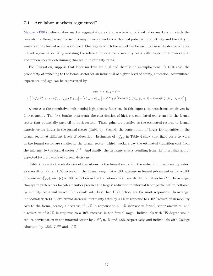
7.1 Are labor markets segmented?

Magnac (1991) defines labor market segmentation as a characteristic of dual labor markets in which the

rewards in different economic sectors may differ for workers with equal potential productivity and the entry of

workers to the formal sector is rationed. One way in which the model can be used to assess the degree of labor

market segmentation is by assessing the relative importance of mobility costs with respect to human capital

and preferences in determining changes in informality rates.

For illustration, suppose that labor markets are dual and there is no unemployment. In that case, the

probability of switching to the formal sector for an individual of a given level of ability, education, accumulated

experience and age can be represented by

P (dt = F |dt−1 = I) =

Λ{[

WFt,k(X

Ft + 1) − γm

2,Ed WIt,k(X

Ft + 1)

]−

[γF3,Ed − γI

3,Ed

]− cI,F + β

[Emax[V F

t+1, VIt+1|dt = F ] − Emax[V F

t+1, VIt+1|dt = I]

]}

where Λ is the cumulative multinomial logit density function. In this expression, transitions are driven by

four elements. The first bracket represents the contribution of higher accumulated experience in the formal

sector that potentially pays off in both sectors. These gains are positive as the estimated returns to formal

experience are larger in the formal sector (Table 6). Second, the contribution of larger job amenities in the

formal sector at different levels of education. Estimates of γm3,Ed in Table 4 show that fixed costs to work

in the formal sector are smaller in the formal sector. Third, workers pay the estimated transition cost from

the informal to the formal sector cI,F . And finally, the dynamic effects resulting from the internalization of

expected future payoffs of current decisions.

Table 7 presents the elasticities of transitions to the formal sector (or the reduction in informality rates)

as a result of: (a) an 10% increase in the formal wage; (b) a 10% increase in formal job amenities (or a 10%

increase in γF3,Ed), and (c) a 10% reduction in the transition costs towards the formal sector cI,F . In average,

changes in preferences for job amenities produce the largest reduction in informal labor participation, followed

by mobility costs and wages. Individuals with Less than High School are the most responsive. In average,

individuals with LHS level would decrease informality rates by 4.1% in response to a 10% reduction in mobility

cost to the formal sector, a decrease of 12% in response to a 10% increase in formal sector amenities, and

a reduction of 2.2% in response to a 10% increase in the formal wage. Individuals with HS degree would

reduce participation in the informal sector by 2.5%, 9.1% and 1.8% respectively, and individuals with College

education by 1.5%, 7.5% and 1.0%.

32

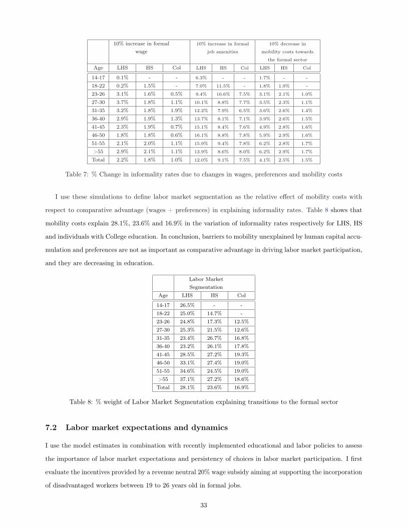
10% increase in formalwage

10% increase in formal

job amenities

10% decrease in

mobility costs towards

the formal sector

Age LHS HS Col LHS HS Col LHS HS Col

14-17 0.1% - - 6.3% - - 1.7% - -

18-22 0.2% 1.5% - 7.0% 11.5% - 1.8% 1.9% -

23-26 3.1% 1.6% 0.5% 9.4% 10.6% 7.5% 3.1% 2.1% 1.0%

27-30 3.7% 1.8% 1.1% 10.1% 8.8% 7.7% 3.5% 2.3% 1.1%

31-35 3.2% 1.8% 1.9% 12.2% 7.9% 6.5% 3.6% 2.6% 1.4%

36-40 2.9% 1.9% 1.3% 13.7% 8.1% 7.1% 3.9% 2.6% 1.5%

41-45 2.3% 1.9% 0.7% 15.1% 8.4% 7.6% 4.9% 2.8% 1.6%

46-50 1.8% 1.8% 0.6% 16.1% 8.8% 7.8% 5.9% 2.9% 1.6%

51-55 2.1% 2.0% 1.1% 15.9% 9.4% 7.8% 6.2% 2.8% 1.7%

>55 2.9% 2.1% 1.1% 13.9% 8.6% 8.0% 6.2% 2.9% 1.7%

Total 2.2% 1.8% 1.0% 12.0% 9.1% 7.5% 4.1% 2.5% 1.5%

Table 7: % Change in informality rates due to changes in wages, preferences and mobility costs

I use these simulations to define labor market segmentation as the relative effect of mobility costs with

respect to comparative advantage (wages + preferences) in explaining informality rates. Table 8 shows that

mobility costs explain 28.1%, 23.6% and 16.9% in the variation of informality rates respectively for LHS, HS

and individuals with College education. In conclusion, barriers to mobility unexplained by human capital accu-

mulation and preferences are not as important as comparative advantage in driving labor market participation,

and they are decreasing in education.

Labor MarketSegmentation

Age LHS HS Col

14-17 26.5% - -18-22 25.0% 14.7% -23-26 24.8% 17.3% 12.5%27-30 25.3% 21.5% 12.6%31-35 23.4% 26.7% 16.8%36-40 23.2% 26.1% 17.8%41-45 28.5% 27.2% 19.3%46-50 33.1% 27.4% 19.0%51-55 34.6% 24.5% 19.0%>55 37.1% 27.2% 18.6%Total 28.1% 23.6% 16.9%

Table 8: % weight of Labor Market Segmentation explaining transitions to the formal sector

7.2 Labor market expectations and dynamics

I use the model estimates in combination with recently implemented educational and labor policies to assess

the importance of labor market expectations and persistency of choices in labor market participation. I first

evaluate the incentives provided by a revenue neutral 20% wage subsidy aiming at supporting the incorporation

of disadvantaged workers between 19 to 26 years old in formal jobs.

33

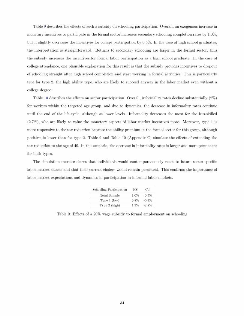
Table 9 describes the effects of such a subsidy on schooling participation. Overall, an exogenous increase in

monetary incentives to participate in the formal sector increases secondary schooling completion rates by 1.0%,

but it slightly decreases the incentives for college participation by 0.5%. In the case of high school graduates,

the interpretation is straightforward. Returns to secondary schooling are larger in the formal sector, thus

the subsidy increases the incentives for formal labor participation as a high school graduate. In the case of

college attendance, one plausible explanation for this result is that the subsidy provides incentives to dropout

of schooling straight after high school completion and start working in formal activities. This is particularly

true for type 2, the high ability type, who are likely to succeed anyway in the labor market even without a

college degree.

Table 10 describes the effects on sector participation. Overall, informality rates decline substantially (2%)

for workers within the targeted age group, and due to dynamics, the decrease in informality rates continue

until the end of the life-cycle, although at lower levels. Informality decreases the most for the less-skilled

(2.7%), who are likely to value the monetary aspects of labor market incentives more. Moreover, type 1 is

more responsive to the tax reduction because the ability premium in the formal sector for this group, although

positive, is lower than for type 2. Table 9 and Table 10 (Appendix C) simulate the effects of extending the

tax reduction to the age of 40. In this scenario, the decrease in informality rates is larger and more permanent

for both types.

The simulation exercise shows that individuals would contemporaneously react to future sector-specific

labor market shocks and that their current choices would remain persistent. This confirms the importance of

labor market expectations and dynamics in participation in informal labor markets.

Schooling Participation HS Col

Total Sample 1.0% -0.5%Type 1 (low) 0.8% -0.3%Type 2 (high) 1.9% -2.8%

Table 9: Effects of a 20% wage subsidy to formal employment on schooling

34

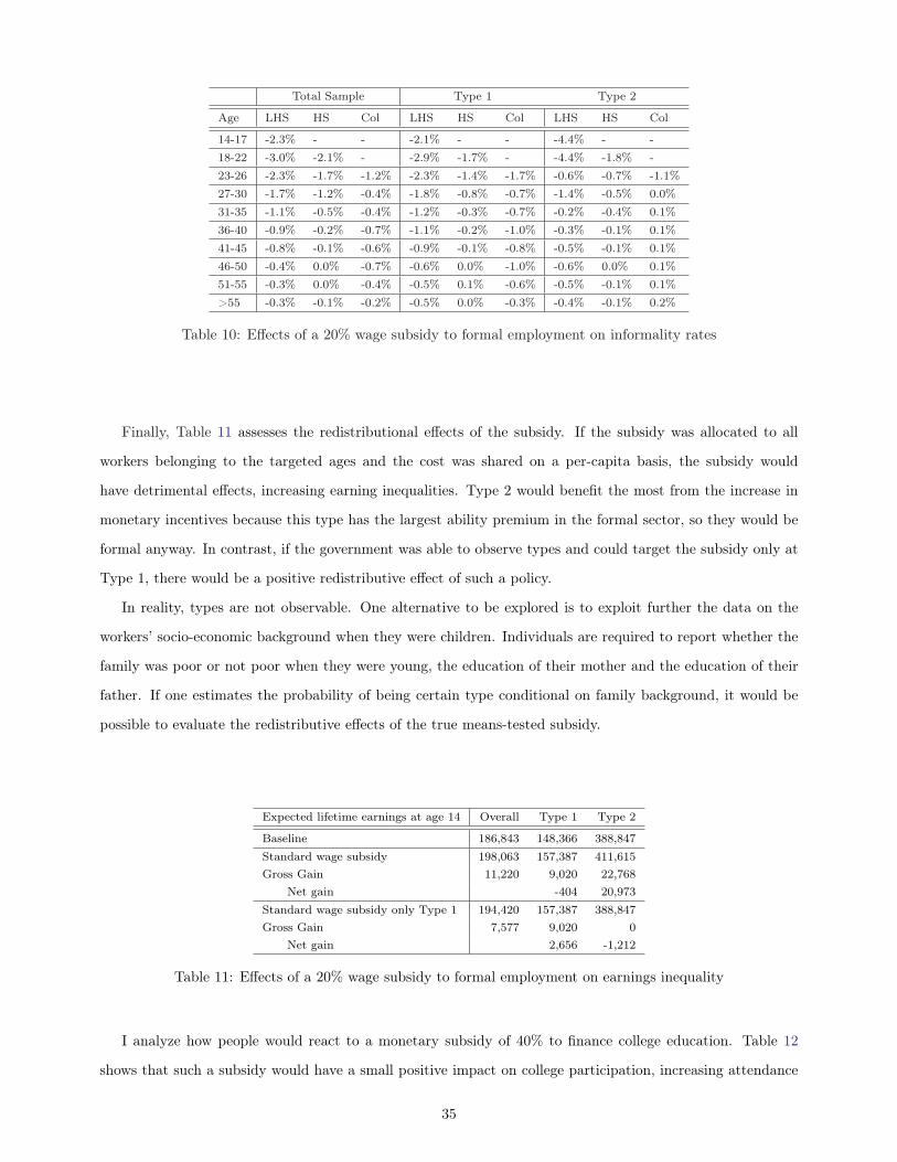
Total Sample Type 1 Type 2

Age LHS HS Col LHS HS Col LHS HS Col

14-17 -2.3% - - -2.1% - - -4.4% - -18-22 -3.0% -2.1% - -2.9% -1.7% - -4.4% -1.8% -23-26 -2.3% -1.7% -1.2% -2.3% -1.4% -1.7% -0.6% -0.7% -1.1%27-30 -1.7% -1.2% -0.4% -1.8% -0.8% -0.7% -1.4% -0.5% 0.0%31-35 -1.1% -0.5% -0.4% -1.2% -0.3% -0.7% -0.2% -0.4% 0.1%36-40 -0.9% -0.2% -0.7% -1.1% -0.2% -1.0% -0.3% -0.1% 0.1%41-45 -0.8% -0.1% -0.6% -0.9% -0.1% -0.8% -0.5% -0.1% 0.1%46-50 -0.4% 0.0% -0.7% -0.6% 0.0% -1.0% -0.6% 0.0% 0.1%51-55 -0.3% 0.0% -0.4% -0.5% 0.1% -0.6% -0.5% -0.1% 0.1%>55 -0.3% -0.1% -0.2% -0.5% 0.0% -0.3% -0.4% -0.1% 0.2%

Table 10: Effects of a 20% wage subsidy to formal employment on informality rates

Finally, Table 11 assesses the redistributional effects of the subsidy. If the subsidy was allocated to all

workers belonging to the targeted ages and the cost was shared on a per-capita basis, the subsidy would

have detrimental effects, increasing earning inequalities. Type 2 would benefit the most from the increase in

monetary incentives because this type has the largest ability premium in the formal sector, so they would be

formal anyway. In contrast, if the government was able to observe types and could target the subsidy only at

Type 1, there would be a positive redistributive effect of such a policy.

In reality, types are not observable. One alternative to be explored is to exploit further the data on the

workers’ socio-economic background when they were children. Individuals are required to report whether the

family was poor or not poor when they were young, the education of their mother and the education of their

father. If one estimates the probability of being certain type conditional on family background, it would be

possible to evaluate the redistributive effects of the true means-tested subsidy.

Expected lifetime earnings at age 14 Overall Type 1 Type 2

Baseline 186,843 148,366 388,847Standard wage subsidy 198,063 157,387 411,615Gross Gain 11,220 9,020 22,768

Net gain -404 20,973Standard wage subsidy only Type 1 194,420 157,387 388,847Gross Gain 7,577 9,020 0

Net gain 2,656 -1,212

Table 11: Effects of a 20% wage subsidy to formal employment on earnings inequality

I analyze how people would react to a monetary subsidy of 40% to finance college education. Table 12

shows that such a subsidy would have a small positive impact on college participation, increasing attendance

35

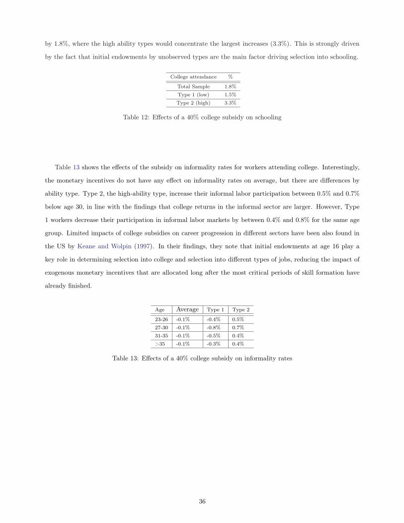
by 1.8%, where the high ability types would concentrate the largest increases (3.3%). This is strongly driven

by the fact that initial endowments by unobserved types are the main factor driving selection into schooling.

College attendance %

Total Sample 1.8%Type 1 (low) 1.5%Type 2 (high) 3.3%

Table 12: Effects of a 40% college subsidy on schooling

Table 13 shows the effects of the subsidy on informality rates for workers attending college. Interestingly,

the monetary incentives do not have any effect on informality rates on average, but there are differences by

ability type. Type 2, the high-ability type, increase their informal labor participation between 0.5% and 0.7%

below age 30, in line with the findings that college returns in the informal sector are larger. However, Type

1 workers decrease their participation in informal labor markets by between 0.4% and 0.8% for the same age

group. Limited impacts of college subsidies on career progression in different sectors have been also found in

the US by Keane and Wolpin (1997). In their findings, they note that initial endowments at age 16 play a

key role in determining selection into college and selection into different types of jobs, reducing the impact of

exogenous monetary incentives that are allocated long after the most critical periods of skill formation have

already finished.

Age Average Type 1 Type 2

23-26 -0.1% -0.4% 0.5%27-30 -0.1% -0.8% 0.7%31-35 -0.1% -0.5% 0.4%>35 -0.1% -0.3% 0.4%

Table 13: Effects of a 40% college subsidy on informality rates

36

8 Concluding Remarks

I contribute to the literature on labor informality in developing countries by studying whether comparative

advantage determines participation in informal labor markets. I develop a life-cycle model building on a Roy

Model extended to endogenous schooling decisions and also extended to compensating wage differentials, to

analyze how individuals with heterogeneous skills and preferences choose schooling and sector participation

based on their comparative advantage. The model is estimated by exploiting rich cross-sectional and time-

varied Chilean panel data on wages, sector participation and school attendance.

My contribution to the literature also relies on the exploration of the different mechanisms by which

comparative advantage might drive choices. First, a structural estimation allows me to disentangle the relative

importance of wage returns and preferences for non-wage attributes in driving decisions. More traditional

approaches used to test whether comparative advantage drives informal labor participation might have some

limitations. For example, the study of wage differentials between the formal and the informal sectors does

not account for the fact that individuals might self-select into jobs based on utility differences, which are not

captured by wages. In addition, studies based on the analysis of mobility rates may not be able to separately

identify whether choices are driven by comparative advantage or if they are a consequence of idiosyncratic or

industry-specific shocks.

Second, some authors have emphasized that a key difference between the formal and informal sectors is

that they are likely to have different production functions. While formal firms are associated with larger

size, higher capital-labor ratios, and higher technology, and demand more skilled labor, informal firms tend to

concentrate unskilled labor-intensive economic activities and operate at lower levels of productivity. I test for

this assumption in a partial equilibrium approach, by estimating skill functions that may vary across sectors.

I show that returns to abilities, schooling and sector-specific experience largely diverge across the formal and

informal sectors. Third, I assess the extent to which labor market expectations matter for decision-making.

Model simulations show that individuals react significantly to labor market expectations by making different

decisions regarding their schooling and participation in informal labor markets when the relative monetary

incentives between the formal and informal sectors change exogenously. The effects of these incentives are per-

sistent over the life-cycle, which indicates the strong effects of dynamics through human capital accumulation.

Finally, I test for the existence of barriers to mobility by estimating transition costs that cannot be explained

by skills, tastes or shocks.

The modeling framework I propose incorporates some innovations. To my knowledge, there is no previous

literature that has studied participation in informal labor markets using a life-cycle approach, in which the

schooling decision is endogenous. Moreover, the previous literature studying labor informality has largely

stressed the importance of heterogeneity in skills and preferences shaping comparative advantage. I explicitly

37

model unobserved heterogeneity by allowing initial endowments to jointly drive selection into schooling and

sector productivity.

Some estimation results are important to highlight. First, the assessment of the relative importance of wage

and sector preferences driving choices shows that both factors are important but there is heterogeneity in the

relative valuation across education. Less educated individuals attach more value to monetary rewards than

non-wage attributes, and the relative valuation of wages for this group is larger in informal activities. These

findings are consistent with previous evidence that less educated informal workers tend to value the possibility

of evading paying taxes and social security contributions from which they derive little value. Instead, more

educated individuals tend to attach more value to the non-wage attributes of jobs relative to wage returns,

and these benefits are larger in the formal sector.

Second, the estimated sector-specific technologies of skill accumulation support the hypothesis that the

formal and informal sectors have different production functions. I find that workers with higher levels of

ability are better rewarded in the formal sector; returns to High School are larger in the formal sector; and, I

find a wage premium in the informal sector for post-secondary schooling. The latter result explains why highly

skilled individuals are found to participate in informal activities despite the fact that, by so doing, they give

up the large non-wage benefits attached to formal contracts. Furthermore, in my sample, more than 90% of

the highly skilled informal workers over the age of 40 are self-employed, which suggests that highly educated

informal workers are actually people involved in successful entrepreneurial activities.

Third, I use the model estimates to assess the importance of labor market expectations for schooling and

labor decisions. I show that a revenue neutral wage subsidy to formal youth employment would decrease

informality by 2% for the targeted age groups, but it would also persistently decrease informality rates for

older workers not affected by the policy, which is a consequence of the dynamic effects of the incentives through

sector-specific human capital accumulation. Furthermore, the subsidy would also increase the incentives to

finish High School (1.5%), and slightly decrease the incentives for college attendance. I also find that the

incentives provided by a college subsidy of 40% would increase college participation by 1.8%, with high-ability

types being the ones who react the most to the incentives (3.3%). On average informality rates would not be

affected, but the policy would significantly reduction informality rates for low-ability types.

And fourth, the estimated transition costs from the informal to the formal sector are substantially larger

than in the opposite direction, while the re-entry costs from non-labor participation in the formal sector are

also larger. Given that, in general, workers prefer to work in formal activities but transitions to this sector

are more costly, I interpret these findings as evidence of the existence of some barriers to entry to the formal

sector.

Finally, my research agenda incorporates two model changes intended to improve the understanding of the

effect of comparative advantage on labor informality. The first improvement relates to the incorporation of

38

self-employment as a third sector. As explained above, informality rates are larger for the elderly because of a

composition effect. While informality for salaried employees decreases over the life-cycle, among the elderly a

larger proportion are self-employed. Figure A.4 in the Appendix shows that if all of the self-employed are now

considered as another sector, the economy is composed of the salaried formal, the salaried informal and the

self-employed, and a clear rank emerges in terms of wage profiles. Remarkably, the formal salaried face higher

wage returns than those in the other two sectors, with slopes increasing in schooling. And while, for individuals

with less than High School level education, the wage profiles for the informal salaried and self-employed are

similar, at higher schooling levels the self-employed become more similar to the formal salaried. This suggests

that the informal salaried and the self-employed have different skill accumulation processes, so it may worth

modeling separately the three different sectors. The estimation of such a model is currently a work in progress.

The second improvement relates to the relaxation of some model assumptions. As discussed above, risk

neutrality is a relatively safe assumption if one is willing to analyze the dynamics for young workers. However,

an interesting extension of the model is the incorporation of risk aversion alongside both private and pension

savings to analyze how schooling and labor supply will change in response to credit market imperfections.

Additionally, in the current modeling framework, I have also assumed that individuals foresee perfectly, the

returns to human capital accumulation across sectors. While most of the literature on dynamic models builds

on this assumption, recent modeling frameworks like the ones proposed by Altonji et al. (2012), emphasize

the importance of incorporating the more realistic assumption that individuals face uncertainty about their

own preferences and the returns to human capital accumulation. I intend to incorporate richer sources of

dynamics in wages and in the paths of human capital accumulation by modeling individuals that learn their

own preferences and the technology of skill formation by doing.

39

References

Adda, J., Dustmann, C., Meghir, C., and Robin, J. (2013). Career Progression, Economic Downturns, and

Skills. NBER Working Paper Series.

Aguirregabiria, V. and Mira, P. (2010). Dynamic discrete choice structural models: A survey. Journal of

Econometrics, 156(1):38–67.

Altonji, J. G., Blom, E., and Meghir, C. (2012). Heterogeneity in Human Capital Investments : High School

Curriculum, College Major, and Careers. NBER Working Paper Series.

Amaral, P. S. and Quintin, E. (2006). A competitive model of the informal sector. Journal of Monetary

Economics, 53(7):1541–1553.

Arbex, M., Galvao, A. F., and Gomes, F. (2010). Heterogeneity in the Returns to Education and Informal

Activities. INSPER Working Papers, pages 1–25.

Attanasio, O., Meghir, C., and Otero, A. (2011). Pensions, Work and Informality:The impact of the 2008

Chilean Pension Reform.

Blundell, R., Costa-Dias, M., Meghir, C., and Shaw, J. (2013). Female Labour Supply, Human Capital and

Welfare Reform. NBER Working Paper Series.

Bosch, M., Goni, E., and Maloney, W. (2007). The Determinants of Rising Informality in Brazil : Evidence

from Gross Worker Flows. IZA Discussion Papers, (2970).

Bosch, M. and Maloney, W. (2007). Comparative Analysis of Labor Market Dynamics Using Markov Processes

: An Application to Informality. IZA Discussion Paper Series, (3038).

Butelmann, A. and Gallego, F. (2000). Household Saving in Chile: Microeconomic Evidence. Banco Central

de Chile Documentos de Trabajo Central Bank of Chile Working Papers.

Contreras, D., Mello, L. D., and Puentes, E. (2008). Tackling Business and Labour Informality in Chile.

OECD Economics Department Working Papers, (607).

Galindev, R. and Lkhagvasuren, D. (2010). Discretization of highly persistent correlated AR(1) shocks. Journal

of Economic Dynamics and Control, 34(7):1260–1276.

Gasparini, L. and Tornarolli, L. (2007). Centro de Estudios Distributivos, Laborales y Sociales.

Gourieroux, C., Monfort, A., and Renault, E. (1993). Indirect Inference C. Gourieroux; A. Monfort; E.

Renault Journal of Applied Econometrics , Vol. 8, Supplement: Special Issue on Econometric Inference

Using Simulation Techniques. (Dec., 1993), pp. S85-S118. Journal of Applied Econometrics, 8.

40

Heckman, J. and Pagés, C. (2003). Law and Employment: Lessons from Latin America and the Caribbean.

NBER Working Paper Series.

Heckman, J. and Singer, B. (1984). A Method for Minimizing the Impact of Distributional Assumptions in

Econometric Models for Duration Data. Econometrica, 52(2):271–320.

Keane, M. and Smith, A. A. (2003). Generalized Indirect Inference for Discrete Choice Models.

Keane, M. P. and Wolpin, K. I. (1997). The Career Decisions of Young Men. Journal of Political Economy,

105(3).

Kennan, J. (2008). Average Switching Costs in Dynamic Logit Models. (January).

Killingsworth, M. R. (1987). Heterogeneous Preferences, Compensating Wage Differentials, and Comparable

Worth. The Quartery Journal of Economics, 102(4):727–742.

Levy, S. (2010). Levy, Santiago. Good intentions, bad outcomes: Social policy, informality, and economic

growth in Mexico. Brookings Institution Press, 2010.

Magnac, T. (1991). Segmented or Competitive Labor Markets. Econometrica, 59(1):165–187.

Magnac, T., Robin, J.-m., and Visser, M. (1999). Analysing Incomplete Individual Employment Histories

Using Indirect Inference. Journal of Applied Econometrics, 10.

Maloney, W. F. (1999). Does Informality Imply Segmentation in Urban Labor Markets? Evidence from

Sectoral Transitions in Mexico. The World Bank Economic Review, 13(2):275–302.

Maloney, W. F. (2004). Informality Revisited. World Development, 32(7):1159–1178.

Meghir, C., Narita, R., and Robin, J.-m. (2012). Wages and Informality in Developing Countries. NBER

Working Paper (Forthcoming American Economic Review).

Meghir, C. and Rivkin, S. (2010). Econometric Methods for Research in Education. National Bureau of

Economic Research.

Moscoso Boedo, H. and D Erasmo, P. (2013). Misallocation , Informality , and Human Capital : Understanding

the Role of Institutions. Virginia Economics Online Papers, (301):1–41.

Pagés, C. and Madrigal, L. (2008). Is Informality a Good Measure of Job Quality ? Evidence from Job

Satisfaction Data by Carmen Pagés. Inter-American Development Bank, (December).

Pagés, C. and Stampini, M. (2007). No Education , No Good Jobs ? Evidence on the Relationship between

Education and Labor Market Segmentation. IZA Discussion Paper Series, (3187).

41

Paula, A. D. and Scheinkman, J. (2007). The Informal Sector : An Equilibrium Model and Some by The

Informal Sector : An Equilibrium Model and Some Empirical Evidence from Brazil. Penn Institute for

Economic Research Working Paper.

Perry, G. (2007). Informality: exit and and exclusion. World Bank-free PDF, 2007.

Tauchen, G. (1986). Finite state markov-chain approximations to univariate and vector autoregressions.

Economics Letters, 20(2):177–181.

Todd, P. E. and Wolpin, K. I. (2010). Structural Estimation and Policy Evaluation in Developing Countries.

Annual Review of Economics, 2(1):21–50.

Willis, R. and Rosen, S. (1979). Eduation and Self-selection. Journal of Political Economy.

Yamada, G. (1996). Urban Informal Employment and Self-Employment in Developing Countries : Theory and

Evidence *. Economic Development and Cultural Change, 44(2):289–314.

42

Appendix

A. Data descriptives

Figure A.1 Informality rates controling by cohort effects.

Figure A.2 Informality rates by schooling females

Figure A.3 Informality rates by schooling

43

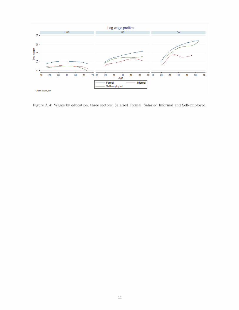
Figure A.4: Wages by education, three sectors: Salaried Formal, Salaried Informal and Self-employed.

44

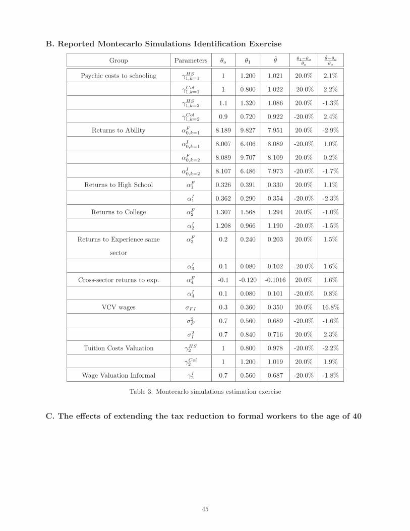
B. Reported Montecarlo Simulations Identification Exercise

Group Parameters θo θ1 θ̂ θ1−θoθo

θ̂−θoθo

Psychic costs to schooling γHS1,k=1 1 1.200 1.021 20.0% 2.1%

γCol1,k=1 1 0.800 1.022 -20.0% 2.2%

γHS1,k=2 1.1 1.320 1.086 20.0% -1.3%

γCol1,k=2 0.9 0.720 0.922 -20.0% 2.4%

Returns to Ability αF0,k=1 8.189 9.827 7.951 20.0% -2.9%

αI0,k=1 8.007 6.406 8.089 -20.0% 1.0%

αF0,k=2 8.089 9.707 8.109 20.0% 0.2%

αI0,k=2 8.107 6.486 7.973 -20.0% -1.7%

Returns to High School αF1 0.326 0.391 0.330 20.0% 1.1%

αI1 0.362 0.290 0.354 -20.0% -2.3%

Returns to College αF2 1.307 1.568 1.294 20.0% -1.0%

αI2 1.208 0.966 1.190 -20.0% -1.5%

Returns to Experience same

sector

αF3 0.2 0.240 0.203 20.0% 1.5%

αI3 0.1 0.080 0.102 -20.0% 1.6%

Cross-sector returns to exp. αF4 -0.1 -0.120 -0.1016 20.0% 1.6%

αI4 0.1 0.080 0.101 -20.0% 0.8%

VCV wages σFI 0.3 0.360 0.350 20.0% 16.8%

σ2F 0.7 0.560 0.689 -20.0% -1.6%

σ2I 0.7 0.840 0.716 20.0% 2.3%

Tuition Costs Valuation γHS2 1 0.800 0.978 -20.0% -2.2%

γCol2 1 1.200 1.019 20.0% 1.9%

Wage Valuation Informal γI2 0.7 0.560 0.687 -20.0% -1.8%

Table 3: Montecarlo simulations estimation exercise

C. The effects of extending the tax reduction to formal workers to the age of 40

45

Age HS Col

Total Sample 1.3% 0.5%

Type 1 (low) 1.5% 0.6%

Type 2 (high) 2.5% -0.2%

Table 9: Extension of tax reduction to age 40 and schooling

Total Sample Type 1 Type 2

Extension LHS HS Col LHS HS Col LHS HS Col

14-17 -2.3% -2.2% -6.8%

18-22 -3.1% -3.1% -3.1% -2.9% -9.0% -2.1%

23-26 -3.1% -3.2% -2.0% -3.1% -3.0% -2.3% -5.6% -1.0% -1.4%

27-30 -2.8% -2.4% -1.7% -3.0% -2.2% -1.8% -2.9% -0.8% -0.4%

31-35 -2.0% -1.7% -2.1% -2.2% -1.5% -2.4% -2.3% -0.7% -0.5%

36-40 -1.9% -1.6% -1.9% -2.2% -1.4% -2.2% -2.1% -0.7% -0.4%

41-45 -1.4% -1.2% -1.7% -1.6% -1.1% -2.1% -1.5% -0.4% -0.1%

46-50 -0.8% -0.7% -1.5% -1.0% -0.7% -1.8% -0.1% -0.2% 0.0%

51-55 -0.5% -0.3% -1.2% -0.7% -0.2% -1.5% -0.1% 0.0% 0.0%

>55 -0.4% -0.3% -0.7% -0.6% -0.2% -0.8% -0.2% -0.1% 0.1%

Table 10: Extension of tax reduction to age 40 and informality

46