John Decatur Version 6.0 10/4/2011

1

HSQC and HMBC for Topspin

These experiments are only possible on the 400 and 500. These experiments can be used to correlate both carbon-proton and nitrogen-proton. The procedure for 15N and any differences from carbon are discussed at the bottom of this handout. HSQC - Heteronuclear Multiple Quantum Correlation. This 2D experiment correlates the chemical shift of proton with the chemical shift of the directly bonded carbon. On the bottom axis is a proton spectrum and on the other is a carbon. Cross peaks give the shift of the corresponding proton and carbon. This experiment utilizes the one-bond coupling between carbon and proton (J=120-215 Hz). HMBC - Heteronuclear Multiple Bond Correlation. This experiment utilizes multiple-bond couplings over two or three bonds (J=2-15Hz. Cross peaks are between protons and carbons that are two or three bonds away (and sometimes up to four or five bonds away). Direct one-bond cross-peaks are suppressed. This experiment is analogous to the proton-proton COSY experiment in that it provides connectivity information over several bonds. 13C HSQC and 13C HMBC spectra of sucrose and 15N HMBC of 1-methylpyrazole are shown at the bottom of this handout. It is useful although not necessary to have already taken a carbon spectrum prior to taking HSQC or HMBC. This 1D can be used as a projection for the 2D. A 1D carbon spectrum, acquired from another NMR (like the 300wb), can be used as a projection. It is faster, however, to acquire an entire 2D HSQC spectrum than a single 1D carbon spectrum and thus, sometimes, it is impossible to obtain a 1D carbon while a 2D HSQC is possible. This is because these 2D experiments are proton-detected and have much higher intrinsic sensitivity than carbon (this is not an effect from the differing abundances of proton and carbon). About sample size, tubes, and sensitivity: When sample quantity is very limited, it is advantageous to limit the amount of solvent in which it is dissolved. If a normal 5mm tube is used, however, this cannot be less than about 500µL without causing serious lineshape (shimming) problems and the attendant loss of signal-to-noise. When one reduces the solvent quantity in a normal 5mm tube, it is important that the sample be centered within the coil. To do this, center the sample about the scored line on the plastic depth gauge. There are special tubes (made by Shigemi) that can be used to restrict the active solvent volume without causing line shape problems. They are available from www.shigemi.com or Aldrich for a higher price. See John Decatur. Choice of HSQC experiments The following HSQC experiments are possible. The choice is made when you read in parameters with the rpar command. I recommend the edited version for normal work but if sensitivity is a concern, then use the standard HSQC. Parmeter set Experiment hsqcedsp.top edited HSQC with CH and CH3 carbons up, CH2 carbons down hsqc.top standard HSQC hsqctocsy.top HSQC-TOCSY – gives a TOCSY spectrum resolved into the carbon dimension

John Decatur Version 6.0 10/4/2011

2

HSQC Procedure 1. Do not spin the sample. Lock, shim and take a normal 1D proton spectrum. Be sure to tune the proton channel of the probe (wobb). Determine the proton spectral region to be used - values of sw and o1p. sw is the spectral width and o1p is the center of the spectrum. For example, if you have peaks over the range 1 to 6 ppm, the optimum region is from 0.5 to 6.5 ppm. Always leave at least 0.5 ppm on the edges of the spectrum. The value for sw is then 6 ppm and o1p is 3.5 ppm. 2. Note the file name of the 1D proton spectra taken above. You may wish to use it as the F2 projection for the 2D plot. 3. Type new to change the filename, or preferably, simply increment the experiment number. 4. Read in the parameters for the HSQC experiment by typing rpar or hsqcedsp.top or hsqc.top. Type getprosol to update the pulse parameters. 5. Type wobb and tune the carbon channel of the probe (The carbon channel comes up on the wobb screen when the HSQC parameters have been read in) 6. The parameters below may be changed. Click AcquPars. The F2 column refers to the proton (direct) dimension and F1 column refers to the carbon (indirect) dimension. The normal range for the carbon spectral width is from 0 -165 ppm since carbonyls do not usually have directly attached protons. If you suspect you have an aldehyde, then the carbon range should increased to include up to 200 ppm or so. • ns - number of scans. By default =1 but this can be increased to give greater signal-to-noise. [the rest are optional] • O1p [ppm] - center of proton spectrum • sw [ppm]for F2 - proton spectral width • O2P [ppm]- center of carbon spectrum • sw [ppm] for F1 - carbon spectral width • td for F1 - # of points in F1 dimension (# of FID's) • fidres - digital resolution. Should be 3-5Hz/pt in F2 . Should be 20-80 Hz/pt in F1. Fidres is given

by the ratio sw/td. Set the values of td in F1 and F2 accordingly. The digital resolution should be set according to your needs, i.e., use better (lower Fidres) resolution if are you interested in carbons that have nearly identical shifts and nearly identical proton shifts. Better digital resolution in F1 dimension requires longer experimental time. Often 80Hz/pt is sufficient.

6. Type expt to determine the time required for the experiment. Values of td in F1 and ns greatly affect the time. 7. Type zg to acquire data. Do not type rga or start. You will see the lock signal fall and rise. This is normal. PROCESSING When data acquisition is complete, type xfb to transform the data. You may transform the data before the acquisition is finished but the resolution of the 2D spectrum will be reduced. (Don't forget to re transform after the experiment is finished). Display control

John Decatur Version 6.0 10/4/2011

3

To expand around a region, simply depress the left mouse button and drag the box around the desired region. To return to the full spectrum, click . To adjust the intensity, use Phasing The HSQC spectrum that you have just run is phase sensitive. You must phase it. An out-of-phase spectrum will look strange and will show dramatic intensity differences on either side of all peaks. To phase a 2D spectrum, one extracts individual 1D rows or columns and phases the 1D spectra. The columns and the rows must both be phased and they must be phased separately. If you have run the edited version, the color of the cross peak indicates the phase and thus the multiplicity. Blue and yellow/green represent opposite phase. CH and CH3 will have one color (yellow/green) and CH2 will have the other (blue). When printing with a black-and-white printer, the color information will have to be added by hand by the user (You!). Click to enter phasing. Phase the rows first. Position the cursor on a row that contains peaks. Click the right mouse button and select add. Then position the cursor on a row with a peak that has a different shift than the first, and right click and select add. The idea is to choose rows such that the peaks cover a

large shift range. You may add more rows but usually two in sufficient. To phase rows, click . There will now be a red line on the largest peak. Adjust its phase using the zero-order button, . Then adjust the phase of other peaks in the other row(s) using the first-order button, . Click to save and return. Click to repeat the above process on columns. The columns will often not need much phase correction. When finished, click to exit phasing. NOTE to MestreNova users: Automatic phasing usually works. Under Processing, phase correction, select “automatic along F2” and then “automatic along F1”. Linear Prediction (optional) Linear prediction is a powerful method of improving the resolution of 2D spectra. Normally the FID in the F1 dimension is not fully sampled –it is cut off. To sample it more completely requires more points (greater TD in F1) and a longer experiment time. Each doubling of TD (in F1) doubles the number of FIDs and thus requires a doubling of experimental time. Linear prediction is a processing method which predicts these cut-off points. It improves resolution in the F1 dimension without any increase in experimental time. It is done after the data is collected and can be optimized by varying the extent of prediction and the NCOEF parameter. It is by default turned off and must be turned on. The price of linear prediction is somewhat lower signal-to-noise. If the signal-to-noise of your spectrum is marginal, then linear prediction is not recommended. Crucial parameters are based on the value of TD (in F1) that was used for the experiment . Click the acqpar tab find this value. The following parameters must be set and are found within the procpar tab: ME_mod : set to LPfr NCOEF: set to 3 times the number of cross peaks in your spectrum. For NOESY spectra, count symmetric peaks as two. Values that are incorrect by more than a factor of two can degrade the resolution. LPBIN: set to 2*TD(in F1) SI (in F1): set to 2*TD(in F1) or 4*TD(in F1) SI is the number of points actually transformed and determines the amount of zero-filling. Caution: Large values of will creat huge data sets. SI should never be smaller than TD (in F1).

John Decatur Version 6.0 10/4/2011

4

To execute linear prediction, you must re-transform the spectrum with xfb. Larger values of LPBIN and SI MAY give even higher resolution. It is possible to use 4*TD for LPBIN and 4*TD for SI. If you make LPBIN larger, also increase the value of SI. Trial and error is necessary to get the optimum spectrum. Linear prediction is normally done only in the F1 dimension. In the F2 dimension, it is better to adjust the digital resolution (Fidres) to the appropriate value before acquiring the spectrum. Shift scale calibration To calibrate, click and set the cross-hairs on a peak for which you know the shift in both dimensions, click the left mouse button, and enter the shifts. Generally, the shift scale will be approximately correct without performing this step. Projections By default, low resolution 1D projections are displayed at the top and left of your spectrum. One can replace the top projection with the high-resolution 1D proton spectrum you took earlier and the left projection with a carbon spectrum. Place the pointer over the projection, right click the mouse, and select external projection. Enter the exact filename as noted in step 2 above (including exact experiment number, etc…) Sometimes, the chemical shifts of the 1D projection do not align with the 2D spectrum. See the above calibration procedure if this is true. Or, you may need to calibrate the 1D spectrum. Peak Picking You may create and annotate a list of peaks in 2D mode. It is easiest using manual mode. Under Analysis, select peak picking. At the bottom of the menu, select start manual picker. Place the cross-hairs directly over a peak and right-click the mouse to add or annotate a peak. One may delete an already selected peak.

When finished, select save, Setting the contour level The Topspin plot editor uses the saved display contour level when it begins. To save the current contour levels, right-click over the spectrum, select edit contour levels, and then simply click OK to close. Plotting See the intro handout for printing. To print using the plot editor, select File, Print. Select “Print with layout – start Plot Editor (plot)”. Select a LAYOUT such as 2Dinv208_11x17 and click OK. This automatically places the proton projection defined in the above step into the spectrum. The carbon projection, however, isn’t brought in automatically. To bring in the carbon projection, one must right-click over the spectrum (within Topspin editor) and select edit. Check the click-box for left projection and then select Left Data Set and then choose a spectrum. To adjust intensities of the projections, right click the mouse over the spectrum and select 1D/2D edit.

These buttons control the projection, To print, select file, print.

HMBC

John Decatur Version 6.0 10/4/2011

5

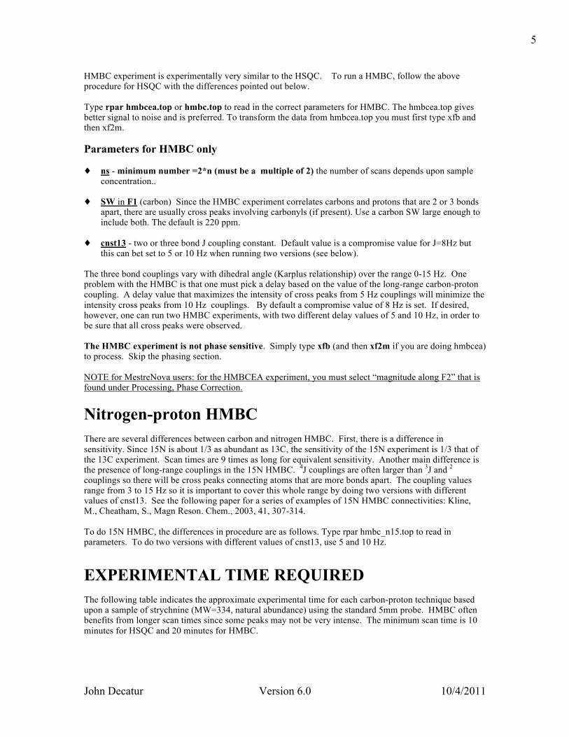
HMBC experiment is experimentally very similar to the HSQC. To run a HMBC, follow the above procedure for HSQC with the differences pointed out below. Type rpar hmbcea.top or hmbc.top to read in the correct parameters for HMBC. The hmbcea.top gives better signal to noise and is preferred. To transform the data from hmbcea.top you must first type xfb and then xf2m. Parameters for HMBC only ♦ ns - minimum number =2*n (must be a multiple of 2) the number of scans depends upon sample

concentration.. ♦ SW in F1 (carbon) Since the HMBC experiment correlates carbons and protons that are 2 or 3 bonds

apart, there are usually cross peaks involving carbonyls (if present). Use a carbon SW large enough to include both. The default is 220 ppm.

♦ cnst13 - two or three bond J coupling constant. Default value is a compromise value for J=8Hz but

this can bet set to 5 or 10 Hz when running two versions (see below). The three bond couplings vary with dihedral angle (Karplus relationship) over the range 0-15 Hz. One problem with the HMBC is that one must pick a delay based on the value of the long-range carbon-proton coupling. A delay value that maximizes the intensity of cross peaks from 5 Hz couplings will minimize the intensity cross peaks from 10 Hz couplings. By default a compromise value of 8 Hz is set. If desired, however, one can run two HMBC experiments, with two different delay values of 5 and 10 Hz, in order to be sure that all cross peaks were observed. The HMBC experiment is not phase sensitive. Simply type xfb (and then xf2m if you are doing hmbcea) to process. Skip the phasing section. NOTE for MestreNova users: for the HMBCEA experiment, you must select “magnitude along F2” that is found under Processing, Phase Correction. Nitrogen-proton HMBC There are several differences between carbon and nitrogen HMBC. First, there is a difference in sensitivity. Since 15N is about 1/3 as abundant as 13C, the sensitivity of the 15N experiment is 1/3 that of the 13C experiment. Scan times are 9 times as long for equivalent sensitivity. Another main difference is the presence of long-range couplings in the 15N HMBC. 4J couplings are often larger than 3J and 2 couplings so there will be cross peaks connecting atoms that are more bonds apart. The coupling values range from 3 to 15 Hz so it is important to cover this whole range by doing two versions with different values of cnst13. See the following paper for a series of examples of 15N HMBC connectivities: Kline, M., Cheatham, S., Magn Reson. Chem., 2003, 41, 307-314. To do 15N HMBC, the differences in procedure are as follows. Type rpar hmbc_n15.top to read in parameters. To do two versions with different values of cnst13, use 5 and 10 Hz.

EXPERIMENTAL TIME REQUIRED The following table indicates the approximate experimental time for each carbon-proton technique based upon a sample of strychnine (MW=334, natural abundance) using the standard 5mm probe. HMBC often benefits from longer scan times since some peaks may not be very intense. The minimum scan time is 10 minutes for HSQC and 20 minutes for HMBC.

John Decatur Version 6.0 10/4/2011

6

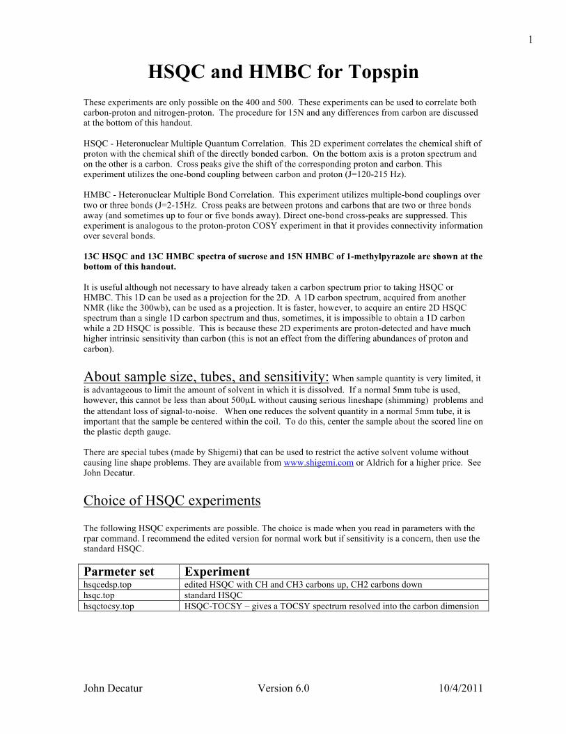
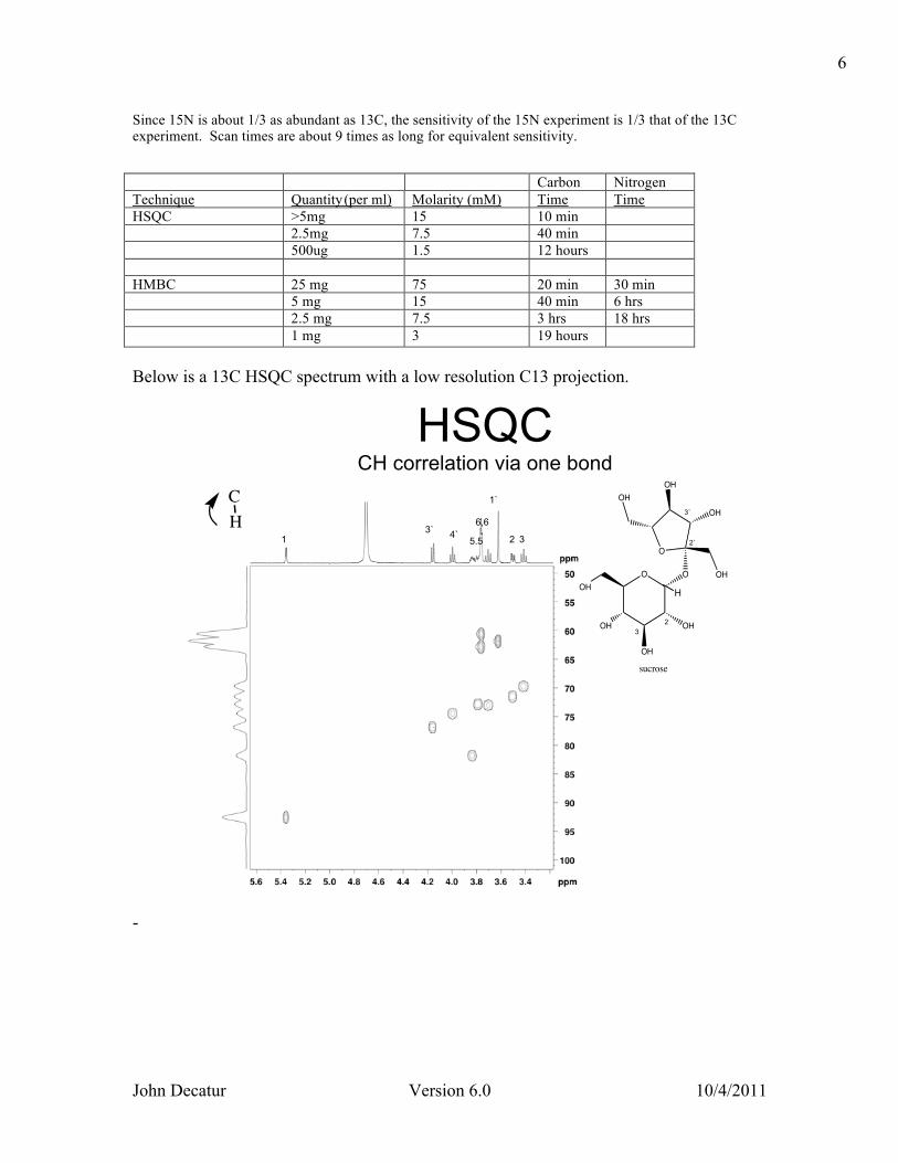
Since 15N is about 1/3 as abundant as 13C, the sensitivity of the 15N experiment is 1/3 that of the 13C experiment. Scan times are about 9 times as long for equivalent sensitivity. Carbon Nitrogen Technique Quantity (per ml) Molarity (mM) Time Time HSQC >5mg 15 10 min 2.5mg 7.5 40 min 500ug 1.5 12 hours HMBC 25 mg 75 20 min 30 min 5 mg 15 40 min 6 hrs 2.5 mg 7.5 3 hrs 18 hrs 1 mg 3 19 hours Below is a 13C HSQC spectrum with a low resolution C13 projection.

-

4 1 2 3 5.5`

1`

3` 4` 6,6`

OH

OH

OH

O

OH

O

OH

OH

OH

OHO

sucrose

H1

2 3

2`

3`

C H

HSQC CH correlation via one bond

John Decatur Version 6.0 10/4/2011

7

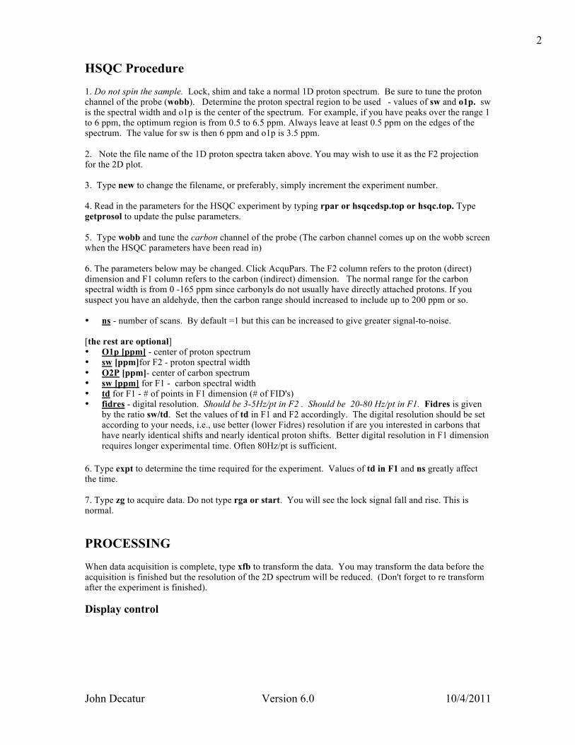
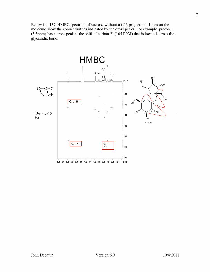
Below is a 13C HMBC spectrum of sucrose without a C13 projection. Lines on the molecule show the connectivitites indicated by the cross peaks. For example, proton 1 (5.3ppm) has a cross peak at the shift of carbon 2’ (105 PPM) that is located across the glycosidic bond.

1`

3 1

C2`- H1

C5,3 - H1

1`

3`

4`

2 4

C2`- H1`

5,5`

3JCH= 0-15 Hz (Karplus)

C CH

C

OH

OH

OH

O

OH

O

OH

OH

OH

OHO

sucrose

H1

2 3

2`

3`

HMBC 6,6`

John Decatur Version 6.0 10/4/2011

8

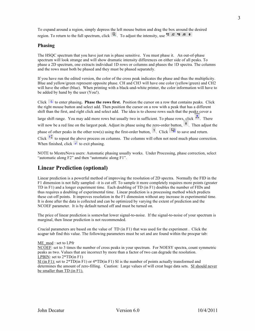
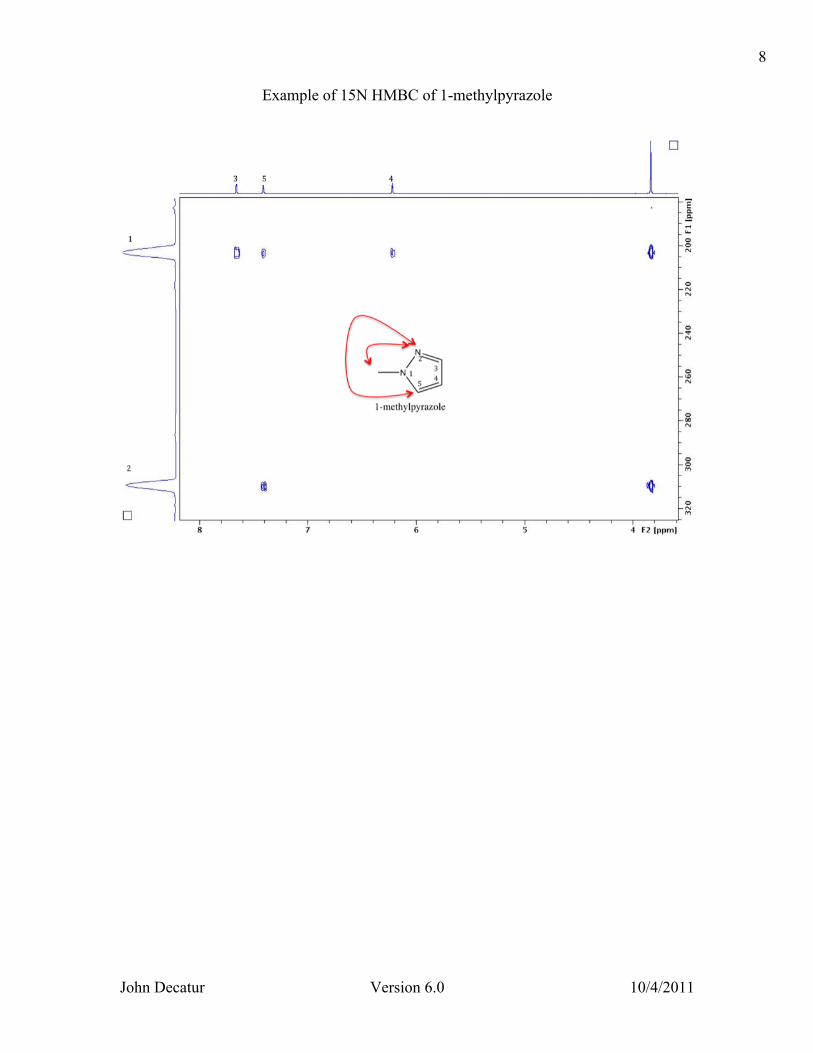
Example of 15N HMBC of 1-methylpyrazole

John Decatur Version 6.0 10/4/2011

9

Non-uniform Sampling for Higher Resolution Non-uniform sampling (NUS) is a method of acquiring 2D data that improves the resolution in the indirect dimension and is now available in Topspin 3, which runs on the 500 and 500 Ascend. In this method, the TD in F1 is made large but not every point is sampled; only a percentage, which is chosen by the user, is sampled. Although only TD*AMOUNT[%] is sampled, the resolution obtained is nearly the same as if TD points were sampled. The sampling percentage is typically 50% but in favorable cases can be as low as 10%. The downside if that the transform (xfb) requires anywhere from 10 minutes to 1 hour and can only be done with Topspin 3 software so far. NUS is similar but superior to using linear prediction for improving resolution. Linear prediction is only a processing technique, while NUS requires collecting the data in a different manner. To acquire NUS mode data: To change ANY experiment from normal mode to NUS mode, read the appropriate parameter set. Then, click AcquPars, and change FnTYPE to non-uniform_sampling. Adjust TD in F1 to be larger than normal, for example, 1024. Click the N in the upper

left panel as shown here, . Adjust the parameter AMOUNT [%} to be 50% or less. Unless you are trying to obtain a 1D 13C spectrum (see below), I recommend 50%. Click A to return. Adjust parameters as normal and type start or zg to acquire. Processing NUS mode data:

1. To transform, type xfb. Between 10 and 60 minutes are required. 2. For phase-sensitive data, you need to give the command xht2 BEFORE phasing.

For HMBCea data, you can then give the xf2m command. Use of HMBC NUS spectra to obtain 1D 13C spectra from mass-limited samples. Carbon spectra from mass limited samples can be difficult to obtain when sample quantities are less than a 1-3 mg or so. HMBC (long-range C-H 2D correlation spectra) are much more sensitive than 13C direct observe spectra. Since quaternary carbons show cross peaks in an HMBC, its 13C projection may have every carbon peak that is present in a standard 13C spectrum. When a standard 13C spectrum is not obtainable due to limited sample, HMBC is a viable alternative. The problem with the 13C projection from a HMBC has been that its resolution has been very low. Its big broad peaks didn’t even look like a 13C spectrum. Improving the projection resolution resulted in a prohibitively long experiment; the number of spectra, td1, had to be increased from 256 to 8K or so. Now with Topspin 3 software, available

John Decatur Version 6.0 10/4/2011

10

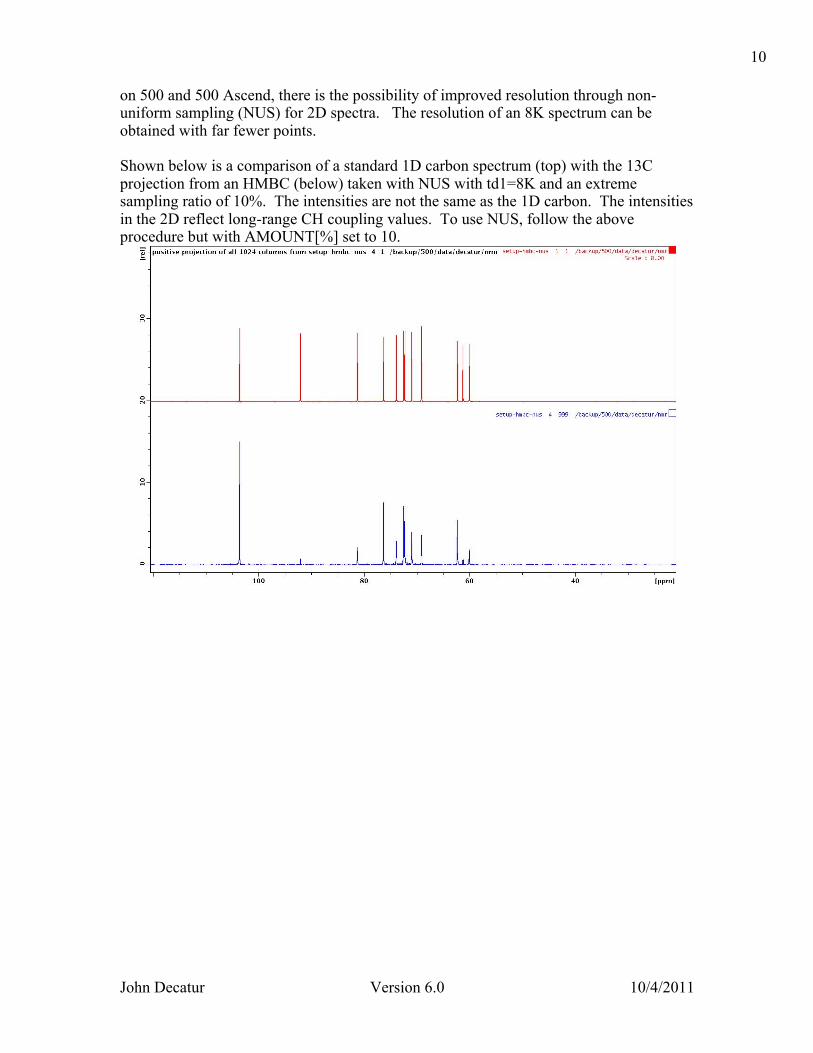
on 500 and 500 Ascend, there is the possibility of improved resolution through non-uniform sampling (NUS) for 2D spectra. The resolution of an 8K spectrum can be obtained with far fewer points. Shown below is a comparison of a standard 1D carbon spectrum (top) with the 13C projection from an HMBC (below) taken with NUS with td1=8K and an extreme sampling ratio of 10%. The intensities are not the same as the 1D carbon. The intensities in the 2D reflect long-range CH coupling values. To use NUS, follow the above procedure but with AMOUNT[%] set to 10.