Embed Size (px)
Citation preview

Engenious Systems, Inc. | UCI Editor 1
2009
Engenious Systems, Inc. Leonard Kong
[HSPF TOOLKIT™] PROGRAM MANUAL REVISION DATE: TUESDAY, DECEMBER 16, 2008
Guide to the program features.


Engenious Systems, Inc. | UCI Editor 3
Table of Contents UCI Editor ...................................................................................................................................................... 1
Project Database ................................................................................................................................... 2
First time start ....................................................................................................................................... 2
Each new Version .................................................................................................................................. 2
Open UCI ................................................................................................................................................... 2
Save UCI .................................................................................................................................................... 3
Save As ...................................................................................................................................................... 3
New UCI .................................................................................................................................................... 3
UCI Snapshot ............................................................................................................................................. 5
Exit Application ......................................................................................................................................... 6
Run HSPF ................................................................................................................................................... 6
Navigating the UCI Document................................................................................................................... 6
Collapsing Outline ................................................................................................................................. 6
Bookmarks ............................................................................................................................................ 6
Block Selection ...................................................................................................................................... 7
Directly manipulating text ........................................................................................................................ 7
Reformat line ........................................................................................................................................ 7
Copy Down ............................................................................................................................................ 8
Auto-Edit Dialog .................................................................................................................................... 9
Comment Toggle ................................................................................................................................. 12
Adding HSPF text ..................................................................................................................................... 12
Add PERLNDS ...................................................................................................................................... 12
Add IMPLNDS ...................................................................................................................................... 14
Add MASSS-LINK ................................................................................................................................. 14
Insert Headers ..................................................................................................................................... 15
EXT SOURCES....................................................................................................................................... 16
Insert New Block ................................................................................................................................. 18
Auto-Create Basins .............................................................................................................................. 19
Extracting Info from UCI.......................................................................................................................... 21
Basin Areas .......................................................................................................................................... 22
4 UCI Editor | Engenious Systems, Inc.
DSN Descriptions ................................................................................................................................. 23
Compare w/DB .................................................................................................................................... 24
HSPF Catalog ........................................................................................................................................... 25
Conversions ............................................................................................................................................. 26
Regional Parameter DB ........................................................................................................................... 27
UCI Specs ................................................................................................................................................. 29
FTABLES ................................................................................................................................................... 29
Lakes.................................................................................................................................................... 29
Storage ................................................................................................................................................ 31
Discharge Controls .............................................................................................................................. 34
FTABLE Lookup .................................................................................................................................... 34
FTABLE Define Section ........................................................................................................................ 35
Wetland ............................................................................................................................................... 37
WDM Utils ................................................................................................................................................... 41
Open WDM ............................................................................................................................................. 41
Close WDM ............................................................................................................................................. 42
Overview ................................................................................................................................................. 42
Statistics .................................................................................................................................................. 42
Rate ..................................................................................................................................................... 43
Volume ................................................................................................................................................ 49
Reports .................................................................................................................................................... 51
Yearly Volume ..................................................................................................................................... 51
Monthly Volume ................................................................................................................................. 52
Daily Rate ............................................................................................................................................ 52
Hourly Rate ......................................................................................................................................... 53
Extract Yearly ...................................................................................................................................... 54
Extract Events...................................................................................................................................... 55
Volume Analysis .................................................................................................................................. 59
Time Series Plotting ............................................................................................................................ 61
DSN Report .......................................................................................................................................... 63
Misc Time Series Tools ............................................................................................................................ 65
Total all points ..................................................................................................................................... 65

Engenious Systems, Inc. | UCI Editor 5
Pond Sizing .......................................................................................................................................... 66
Compliance ......................................................................................................................................... 73
Water Quality ...................................................................................................................................... 76
New WDM ........................................................................................................................................... 77
Schematic Layout ........................................................................................................................................ 81
SUBBSN nodes ......................................................................................................................................... 82
Navigation ............................................................................................................................................... 85
Rename ............................................................................................................................................... 85
Select All .............................................................................................................................................. 85
Transform to Edge ............................................................................................................................... 85
Hide Copy Nodes ................................................................................................................................. 85
Hide Standalone Nodes ....................................................................................................................... 85
Clear Schematic ................................................................................................................................... 85
Find Schematic .................................................................................................................................... 85
Find Node ............................................................................................................................................ 85
Basin Dialog ............................................................................................................................................. 85
RCHRES Dialog ......................................................................................................................................... 85
Copy Dialog ............................................................................................................................................. 85
POA Dialog .............................................................................................................................................. 85
Miscellaneous Tools .................................................................................................................................... 87
Clipboard ................................................................................................................................................. 87
Extract Column From Clipboard .............................................................................................................. 88
Tab to FTABLE ......................................................................................................................................... 88
Stage Lookup ........................................................................................................................................... 88
Flow From Stage ..................................................................................................................................... 88
View Ascii File .......................................................................................................................................... 88
Preferences ............................................................................................................................................. 88
External Programs ............................................................................................................................... 88
Misc Options ....................................................................................................................................... 90
Frequency Compliance ........................................................................................................................ 91
Default Attributes ............................................................................................................................... 91
Soils Logs ................................................................................................................................................. 92
6 UCI Editor | Engenious Systems, Inc.
Other ........................................................................................................................................................... 93
HSPF Documentation .............................................................................................................................. 93
WDMUtil Documentation ....................................................................................................................... 93
About....................................................................................................................................................... 93
Registration ............................................................................................................................................. 93
Server URL ............................................................................................................................................... 93
Revision Log ............................................................................................................................................ 93
Equations .................................................................................................................................................... 99
Vault ........................................................................................................................................................ 99
Trapezoidal .............................................................................................................................................. 99
Underground Pipe ................................................................................................................................... 99
Circular .............................................................................................................................................. 100
Arch ................................................................................................................................................... 100
Ellipse ................................................................................................................................................ 100
Stage-Storage ........................................................................................................................................ 100
Rectangular Weir .................................................................................................................................. 101
Vee ........................................................................................................................................................ 102
Multiple Orifice ..................................................................................................................................... 104
Vertical .................................................................................................................................................. 105
Overflow Riser ....................................................................................................................................... 106
Orifice Eqn: ........................................................................................................................................ 106
Weir Equation: .................................................................................................................................. 107
HSPFToolKit for Reviewers ........................................................................................................................ 111
Basin Areas Report ................................................................................................................................ 111
Regional Parameter Comparison .......................................................................................................... 111
FTable Comparison ............................................................................................................................... 111
DSN Totals Comparison......................................................................................................................... 111
Water Quality Target ............................................................................................................................ 111
References ................................................................................................................................................ 115

Engenious Systems, Inc. | UCI Editor 7
Figures
Figure 1-Editor Colors ................................................................................................................................... 1
Figure 2-New UCI .......................................................................................................................................... 3
Figure 3-UCI Document ................................................................................................................................. 4
Figure 4-EXT SOURCES from New UCI ........................................................................................................... 4
Figure 5-Snap Shot Dialog ............................................................................................................................. 5
Figure 6- Example of Outline Bar .................................................................................................................. 6
Figure 7- Example Bookmark ........................................................................................................................ 7
Figure 8-Quick Block Selector ....................................................................................................................... 7
Figure 9 -Random file name positioning ....................................................................................................... 7
Figure 10-Reformatted line ........................................................................................................................... 8
Figure 11-Copy Down initial data .................................................................................................................. 8
Figure 12-Copy Down with changed initial value at top of column .............................................................. 8
Figure 13-Copy Down after command .......................................................................................................... 8
Figure 14-Sample of status bar for LSUR variable ........................................................................................ 9
Figure 15-Activity window ............................................................................................................................ 9
Figure 16-PWAT-STATE1 sub block ............................................................................................................. 10
Figure 17-General Editor Dialog .................................................................................................................. 10
Figure 18-Dfts as Spaces unchecked and Correct Dfts checked ................................................................. 10
Figure 19-Both fields checked ..................................................................................................................... 10
Figure 20-Uncheck Correct Dfts and Check Dfts As Spaces ........................................................................ 11
Figure 21- Global Block Editor ..................................................................................................................... 11
Figure 22-INGRP Op Editor .......................................................................................................................... 11
Figure 23- Add PERLND ............................................................................................................................... 12
Figure 24- Use Regional Parameters unchecked ........................................................................................ 13
Figure 25- affect of using non-regionalize parameters. .............................................................................. 13
Figure 26- Add PERLND pop up. .................................................................................................................. 14
Figure 27- MASS-LINK Editor ....................................................................................................................... 15
Figure 28- Insert MASS-LINK Block 4 ........................................................................................................... 15
Figure 29- Insert Header ............................................................................................................................. 16
Figure 30- Block with Inserted Header ....................................................................................................... 16
Figure 31-Sample FILE BLOCK for EXT SOURCES dialog .............................................................................. 17
Figure 32-EXT SOURCES dialog ................................................................................................................... 17
Figure 33-GLOBAL BLOCK before pasting ................................................................................................... 18
Figure 34-Sample of EXT SOURCES lines for pasting. .................................................................................. 18
Figure 35-Insert UCI Block ........................................................................................................................... 19
Figure 36-Block after pasted into document. ............................................................................................. 19
Figure 37- Sample commented SCHEMATIC block ..................................................................................... 19
Figure 38- Example SUBBSN Block .............................................................................................................. 20

8 UCI Editor | Engenious Systems, Inc.
Figure 39- Collapsed SUBBSN block ............................................................................................................ 20
Figure 40- Collapsed Block with Basin Description omitted from END tag ................................................ 20
Figure 41-SCHEMATIC Block before Auto-Create Command...................................................................... 20
Figure 42 – Auto Create Basins ................................................................................................................... 21
Figure 43-User Modified SUBBSN tags ....................................................................................................... 21
Figure 45- Example Basin Summary Report ................................................................................................ 22
Figure 44 – Basin Area Dialog Results. ........................................................................................................ 22
Figure 46- Example of EXT TARGETS Block ................................................................................................. 23
Figure 47- DSN Assignments ....................................................................................................................... 23
Figure 48- Example GEN-INFO from PERLND block .................................................................................... 24
Figure 49- Sample Regional Parameter Comparison .................................................................................. 25
Figure 50- Sample report with different land use titles .............................................................................. 25
Figure 51- HSPF Catalog .............................................................................................................................. 26
Figure 52- Sample of Conversions Dialog ................................................................................................... 27
Figure 53-Regional Parameter Editor ......................................................................................................... 28
Figure 54- Pond Sizing Dialog ...................................................................................................................... 30
Figure 55-Sample of FTABLE generated by Pond Sizing Worksheet ........................................................... 31
Figure 56- Sand Filter Example ................................................................................................................... 32
Figure 57- Sand Filter Tab ........................................................................................................................... 33
Figure 58 - Gravel Trench ............................................................................................................................ 33
Figure 59 - Ksat option of Infiltration .......................................................................................................... 34
Figure 60- Sample FTABLE Lookup .............................................................................................................. 35
Figure 61- Channel Section ......................................................................................................................... 36
Figure 62-Manning's Number selection ...................................................................................................... 36
Figure 63 - Wetland GEN-INFO ................................................................................................................... 37
Figure 64-Wetland, PWAT-PARM6 and PARM7.......................................................................................... 38
Figure 65-Wetland, Cursor on PERLND 37 .................................................................................................. 38
Figure 66-Wetland Dialog ........................................................................................................................... 39
Figure 67- Open WDM ................................................................................................................................ 41
Figure 68- WDM Display ............................................................................................................................. 42
Figure 69= Data Set Summary ..................................................................................................................... 42
Figure 70- Sample Log Pearson Plot ........................................................................................................... 43
Figure 71 - Computation of Summations .................................................................................................... 44
Figure 72 - Log Pearson Type III Return Frequencies .................................................................................. 45
Figure 73 - Log Pearson Confidence limits. ................................................................................................. 45
Figure 74 - Sample Peak Yearly Flow Report .............................................................................................. 46
Figure 75 - Ranked Peak Yearly Report ....................................................................................................... 46
Figure 76 - Years Closest to Return Frequency Rate ................................................................................... 47
Figure 77 - Gringorton Plotting Positioning ................................................................................................ 48
Figure 78- Export Return Frequencies to StormShed3G ............................................................................. 48
Figure 79- Example Return Frequency by Volume table. ........................................................................... 49
Figure 80- Total Yearly Volume ................................................................................................................... 50

Engenious Systems, Inc. | UCI Editor 9
Figure 81-Ranked Total Volume Report ...................................................................................................... 50
Figure 82- Frequency Years Volume Report ............................................................................................... 51
Figure 83- Peak Yearly Volume Report ....................................................................................................... 52
Figure 84- Monthly Volume Report ............................................................................................................ 52
Figure 85- Excel Report of Daily Rate .......................................................................................................... 53
Figure 86- Hourly Rate data in EXCEL ......................................................................................................... 53
Figure 87- ASCII File format for hourly rates. ............................................................................................. 53
Figure 88- Extract Yearly TS ........................................................................................................................ 54
Figure 89- Pasting data to EXCEL ................................................................................................................ 55
Figure 90- Pasted EXCEL Yearly Time Series ............................................................................................... 55
Figure 91- Extract By Volume Event Duration ............................................................................................ 56
Figure 92- Example filename for CSV extraction ........................................................................................ 56
Figure 93 - Example Html Extraction of Peak Volumes ............................................................................... 57
Figure 94- StormShed3G hydrographs from HSPFToolkit ........................................................................... 57
Figure 95- StormShed3G 7 Day hydrograph plot ........................................................................................ 58
Figure 96- StormShed3G Application Links Location .................................................................................. 58
Figure 97- First Several Lines of RAC file ..................................................................................................... 59
Figure 98- Example of TS format time series in StormShed3G ................................................................... 59
Figure 99- Summary Return Freq by Log Pearson Type III .......................................................................... 60
Figure 100-Peak Volume Durations for DSN: 801 ....................................................................................... 61
Figure 101- TS Plot for DSN 701 and DSN 801 ............................................................................................ 62
Figure 102- Sample TS Plot selecting both Precipitation and Runoff Time Series ...................................... 62
Figure 103-Sample DSN Report Dialog Box................................................................................................. 63
Figure 104- DSN automatically selected by Test Report 1 .......................................................................... 64
Figure 105-Sample of generated report using the DSN Report feature ..................................................... 65
Figure 106-Pond Sizing Screen 1 ................................................................................................................. 66
Figure 107- Example showing the infiltration rate explicitly set for Pond Estimator ................................. 67
Figure 108- Initial Trap Pond Settings ......................................................................................................... 68
Figure 109 - Pond Size Estimator ................................................................................................................ 68
Figure 110 - Pond Estimator Results ........................................................................................................... 69
Figure 111-Discharge Structure Configuration ........................................................................................... 70
Figure 112 - Results Plot 1........................................................................................................................... 70
Figure 113- Results Plot 2 ........................................................................................................................... 71
Figure 114- Final Routing Results ................................................................................................................ 71
Figure 115- Close up of the Plot .................................................................................................................. 71
Figure 116 - Chart view of Routing results. ................................................................................................. 72
Figure 117-Change Increment and Decimal places .................................................................................... 72
Figure 118-Compliance Plot information panel .......................................................................................... 72
Figure 119- Sample FTABLE Report ............................................................................................................. 73
Figure 120- Compliance Dialog ................................................................................................................... 74
Figure 121- Compliance Chart .................................................................................................................... 75
Figure 122-WDM Report View show Compliance ...................................................................................... 75

10 UCI Editor | Engenious Systems, Inc.
Figure 123- Water Quality Calculator ......................................................................................................... 76
Figure 124 - Water Quality Computation. .................................................................................................. 77
Figure 125-Example of UCI that specifies two WDM files .......................................................................... 77
Figure 126-Create WDM ............................................................................................................................. 78
Figure 127- Adding a DSN to a WDM File ................................................................................................... 78
Figure 128- Auto Layout Create .................................................................................................................. 81
Figure 129- Layout Example 1 ..................................................................................................................... 82
Figure 130- Layout 1 Cleaned up ................................................................................................................ 82
Figure 131 - Basin Dialog ............................................................................................................................. 83
Figure 132- Schematic Block for example layout. ....................................................................................... 84
Figure 133 - Layout 3................................................................................................................................... 84
Figure 134- MASS LINK 15 ........................................................................................................................... 84
Figure 135-Sample Space-Tab Transform ................................................................................................... 87
Figure 136-EXCEL Paste ............................................................................................................................... 87
Figure 137-Generic Parse. ........................................................................................................................... 88
Figure 138 - External Programs ................................................................................................................... 89
Figure 139- Misc Options, Preference Dialog ............................................................................................. 90
Figure 140- Preferences Frequency Compliance ........................................................................................ 91
Figure 141- Preferences, Default Attributes ............................................................................................... 91
Figure 142: Rectangular Weir ................................................................................................................... 101
Figure 143: Triangular or Vee Weir ........................................................................................................... 103
Engenious Systems, Inc. | UCI Editor 1
UCI Editor The UCI Editor is the nothing more than a text editor that has been customized to make editing an HSPF
UCI (User Control Input) file easier. It blurs the distinction between a traditional “front end” type
interfaces in which all input is managed by input dialog boxes and no interface at all with a programming
language.
The traditional method of running HSPF is by creating a text file that contains the specifications for what
is to be computed. Running HSPF is really programming in its purest sense. The HSPF project needed to
be programmed to perform the desired computations.
Modern day programming surprisingly remains in the format of text files, however, the text files are
created with customized editors that have the ability to collapse sections of text, apply color to different
groups of text syntactically, and enforce rules related to the programming language syntax. HSPFToolkit
attempts to do much of the same for the UCI language.
The UCI Editor has the ability to collapse the major HSPF Groups. The editor automatically distinguishes
between command line and comment lines. It knows what type of text is associated with each data
group and knows the position of each data field associated with the group.
The editor also provides basic information associated with each cursor location in the UCI file. If the
cursor is situated where a particular HSPF variable should be placed, the status line at the bottom of the
program window will display the cursors line and column number along with the controlling HSPF Block,
variable name and the variables start column position, the number of spaces available for the variable.
If appropriate, it will also display the default, minimum and maximum values for the field.
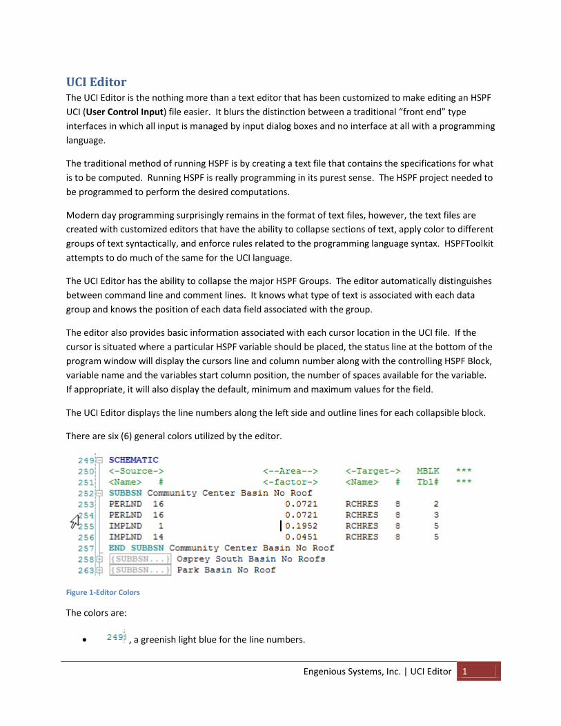
The UCI Editor displays the line numbers along the left side and outline lines for each collapsible block.
There are six (6) general colors utilized by the editor.
Figure 1-Editor Colors
The colors are:
, a greenish light blue for the line numbers.

2 UCI Editor | Engenious Systems, Inc.
, a navy blue for Major Block Names.
, a light green for comments.
, a heavy blue-green for the sub basin block.
, a light gray for collapsed text.
Black for normal text.
Project Database
Each UCI file is paired with an HSPFToolkit project database. For the most part, this database can be
deleted at any time outside of the program (via Windows). It will automatically be recreated the next
time the UCI file is opened. The only time when its deletion might present a huge inconvenience is if
there is a Schematic Layout associated with the UCI File.
When that is the case, the Schematic will have to be re-created.
Deletion of the project database will also delete all the saved UCI Scenarios. This is not a problem if you
don’t need them or they can be easily re-created. It is, if they are vital to your project.
First time start
The first time HSPFToolkit is started, a Preferences Dialog box will appear. See the Preferences section
under Miscellaneous Tools for more information. In general, the program will work even if no
preferences are set.
The dialog will reappear each time the program starts until it is satisfied.
Each new Version
The program is distributed on-line and managed by out remote servers. Each time the program is
started, the license is authenticated and the servers are checked for updates. If there is a new version of
the program, a Revision Dialog box will appear. The dialog box is a history of revisions.
Open UCI The Open UCI menu selection presents a standard windows based dialog for UCI file selection.
HSPFToolkit will open to the last directory where a UCI file was selected. It will not automatically select
the last UCI file that was opened.
If a UCI file is currently opened, it will automatically be saved and closed. A unique feature of the editor
is the ability automatically saved the contents of the UCI file to a database when it is opened. The
“original” contents can then be recalled at any time during the session. The primary reason for this
feature is to enable recovery of the starting version.
HSPFToolkit automatically saves the UCI before running the HSPF program. When this could be a
problem if changes were made and an HSPF run was attempted that was not satisfactory. The UCI file
was automatically saved and altered. With the Scenario Database, the initial version could easily be
recovered. See the section on the UCI Snapshot for additional information.

Engenious Systems, Inc. | UCI Editor 3
Save UCI There is nothing special about this feature. The program saves the UCI document to its current file
name. If a WDM database is opened, that is not saved as part of the UCI save command.
Save As The standard Save-As dialog is presented.
New UCI This feature creates a UCI document from scratch.
Figure 2-New UCI
When the dialog is opened, it is not filled out. The user has the option of manually selecting the blocks
and sub blocks that are to be included in the new UCI document, or a template can be selected.
Currently, there is only single template available. It is the Basic Runoff Analysis template.
Once the template is selected, the user can modify the selection of blocks. If the user has a WDM that
contains the precipitation and evaporation time series, it may be selected. In this scenario, the UCI
document is intended to have Two WDM databases associated with it. The first is the WDM database
that specifies the precipitation and evaporation time series. The second is the WDM database that
contains the time series generated by the UCI document.
When a WDM file is selected time series with the TSTYPE attribute PREC and PETIN are separated into
two (2) selection boxes. As a minimum, if a time series from the WDM file is used, it must be the
Precipitation time series. The Evaporation times series may be omitted (either or both are selected with
the and check boxes). The selection of the precipitation and evaporation time
4 UCI Editor | Engenious Systems, Inc.
series will automatically update the starting and ending dates to present the date range that are
common to both time series.
From a modeling stand point, this range is the largest possible date range for the analysis period. It is
probably not the best date range. If the analysis is for yearly time series, then it would be best to adjust
the starting and ending date to represent complete years.
The program cannot help the user in determining the multiplier for either the precipitation factor or the
evaporation factor. Those are site dependent. If it is not known, leave them a one (1) and adjust the
values in the UCI at a later time. The adjustment is in the EXT SOURCES block.
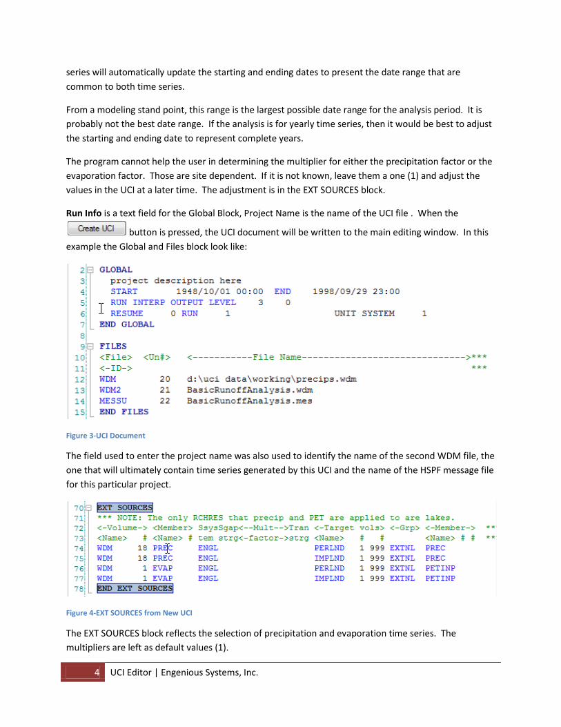
Run Info is a text field for the Global Block, Project Name is the name of the UCI file . When the
button is pressed, the UCI document will be written to the main editing window. In this
example the Global and Files block look like:
Figure 3-UCI Document
The field used to enter the project name was also used to identify the name of the second WDM file, the
one that will ultimately contain time series generated by this UCI and the name of the HSPF message file
for this particular project.
Figure 4-EXT SOURCES from New UCI
The EXT SOURCES block reflects the selection of precipitation and evaporation time series. The
multipliers are left as default values (1).
Engenious Systems, Inc. | UCI Editor 5
In the case of this example, modifications to the block selection set can be saved by simply pressing the
button. The current template name can also be updated by modifying the
field.
If the check box is checked, the Rename Template field changes to
, and the button becomes enabled. Assign a new
template name to the current block selection set and press the button.
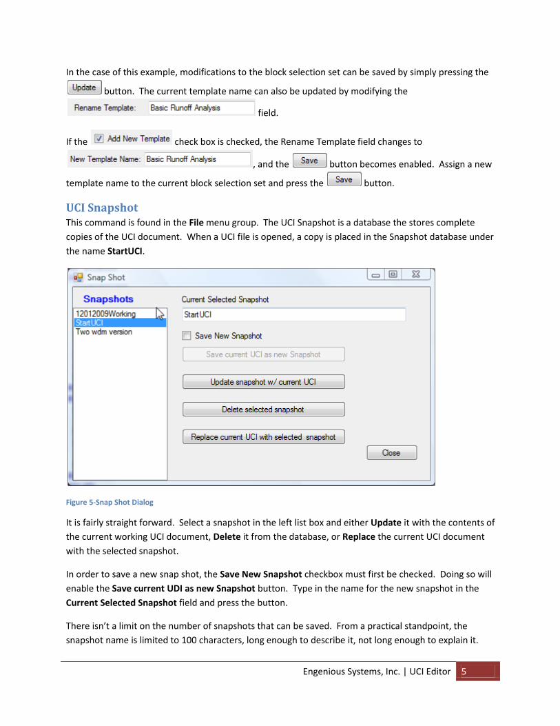
UCI Snapshot This command is found in the File menu group. The UCI Snapshot is a database the stores complete
copies of the UCI document. When a UCI file is opened, a copy is placed in the Snapshot database under
the name StartUCI.
Figure 5-Snap Shot Dialog
It is fairly straight forward. Select a snapshot in the left list box and either Update it with the contents of
the current working UCI document, Delete it from the database, or Replace the current UCI document
with the selected snapshot.
In order to save a new snap shot, the Save New Snapshot checkbox must first be checked. Doing so will
enable the Save current UDI as new Snapshot button. Type in the name for the new snapshot in the
Current Selected Snapshot field and press the button.
There isn’t a limit on the number of snapshots that can be saved. From a practical standpoint, the
snapshot name is limited to 100 characters, long enough to describe it, not long enough to explain it.

6 UCI Editor | Engenious Systems, Inc.
Exit Application This closes both the UCI Document and the WDM database if they are opened.
Run HSPF If a UCI file is opened, the program will run HSPF passing the UCI File as an argument. Theoretically, the
toolkit supports any version of HSPF that allows the UCI file to be passed as a command line argument.
The most common version of HSPF is WinHSPFLite™ available with the BASIN distribution of HSPF from
the USGS.
HSPFToolkit must know where to find the implementation of HSPF in order to process the UCI File. That
is done by the Preferences Dialog.
Navigating the UCI Document Navigating the UCI document is like navigating in any editor, except that this editor has been customized
for HSPF. There are some features that are provided to enhance the experience.
Collapsing Outline
The Editor has collapsible outlines. What this means is that whole sections can be collapsed to “hide”
lines that might not be of immediate interest. Since this is an HSPF editor, the collapsible sections have
been set as all the major HSPF blocks and sub-blocks.
To help manage the document, two (2) buttons ( ) are provided on the tool bar. These buttons
either collapses all blocks or opens all blocks. Generally, the button is used to collapse the entire
document and individual blocks are un-collapsed as needed.
In the collapsed state a block is displayed in a light gray with a + symbol next to it, such as for the
collapsed Global block, . Click on the + symbol to un-collapse the section of text.
Figure 6- Example of Outline Bar
In the un-collapsed state, there is a light gray vertical outline bar showing the extent of the outline
block.
Bookmarks
The program supports bookmarks. Bookmarks are place holders that can be set in order to quickly
return to its location. Bookmarks are supported by four (4) buttons ( ) on the toolbar.

Engenious Systems, Inc. | UCI Editor 7
The buttons are to toggle a bookmark, move to the next bookmark, move to the previous bookmark or
remove all bookmarks. When a line is bookmarked, a turquoise shape is place on the frame.
Figure 7- Example Bookmark
Line 60 in the above figure has been bookmarked.
Block Selection
Another way to navigate the UCI document is to use the quick block locator drop down.
This is a drop down selector located on the toolbar. It contains a list
of all major HSPF blocks. Simply select the block and the editor will
jump to the beginning of the block.
Figure 8-Quick Block Selector
Directly manipulating text The UCI Editor also assists in directly manipulating text. That is, when possible, assistance is available as
an alternative for typing something into the editor. This is important, particularly in the case of a UCI
document where all text must be position in a specific range of spaces.
HSPF expects that the UCI document contain no more than 80 characters on a line. Data fields are
located at specific character positions based on the block that it occupies. The size of the data field
varies depending on the variable that is expected. Most users welcome any type of help that might be
available.
Reformat line
When the mouse cursor is situated on a line within a block that is recognized, right mouse clicking will
present a context defined menu. That means the content of the menu varies depending on the block.
In any case, one of the possible menu selections is Reformat Line. Select the menu and the line will be
reformatted. Consider the file name field in the Files Block. It is large and the file name can be
positioned anywhere within the allowable field.
Figure 9 -Random file name positioning
By right mouse clicking anywhere on the line and selecting Reformat Line, the fields will be reformatted.
8 UCI Editor | Engenious Systems, Inc.
Figure 10-Reformatted line
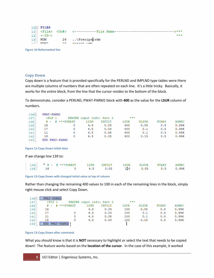
Copy Down
Copy down is a feature that is provided specifically for the PERLND and IMPLND type tables were there
are multiple columns of numbers that are often repeated on each line. It’s a little tricky. Basically, it
works for the entire block, from the line that the cursor resides to the bottom of the block.
To demonstrate, consider a PERLND, PWAT-PARM2 block with 400 as the value for the LSUR column of
numbers.
Figure 11-Copy Down initial data
If we change line 139 to:
Figure 12-Copy Down with changed initial value at top of column
Rather than changing the remaining 400 values to 100 in each of the remaining lines in the block, simply
right mouse click and select Copy Down.
Figure 13-Copy Down after command
What you should know is that it is NOT necessary to highlight or select the text that needs to be copied
down! The feature works based on the location of the cursor. In the case of this example, it worked

Engenious Systems, Inc. | UCI Editor 9
immediately because we only changed the 4 with 1 and the position of the mouse cursor was between
the 1 and 0 (see Figure 12). If the position of the mouse cursor were after the last zero in 100, it would
technically be in the next field (the SLSUR field), so it would not work!
The only requirement for this feature to work is that the cursor is in the field allotted for the variable.
The text should not be selected and in fact, the cursor does not even have to be touching the text within
the field!
How do you know where the field for the variable it? Generally, the green headers will give you some
indication. Another way is to look at the status bar along the bottom of the program frame. In the case
of Figure 12, looking at the program frame:
Figure 14-Sample of status bar for LSUR variable
Here we see that the cursor is on line 138, column 48 in the LSUR variable. The variable starts at column
40 and has a width of 10 characters.
Auto-Edit Dialog
Double-clicking on any line with in any block in the editor will probably present a dialog for data entry
that is an alternate to simply typing text. Most of the time, it is a general editing dialog box that displays
a single row of text in fields assigned to each variable in the row.
When the field is a simple yes/no field, then a check box is presented, otherwise, it is a field where data
can be typed.
Double clicking on a row in the ACTIVITY sub block will present:
Figure 15-Activity window
This is pretty simple. Make any changes and press the Update button, otherwise the red x at the upper
right corner to close. Other rows are not so obvious. Assume a line in the PWAT-STATE1 sub block is
clicked.
10 UCI Editor | Engenious Systems, Inc.
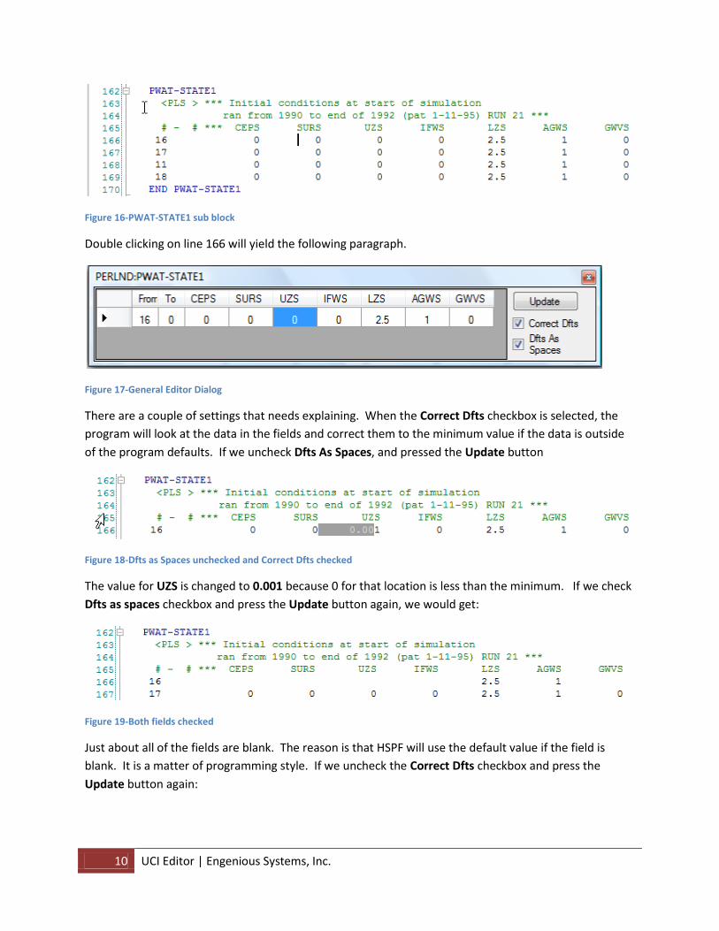
Figure 16-PWAT-STATE1 sub block
Double clicking on line 166 will yield the following paragraph.
Figure 17-General Editor Dialog
There are a couple of settings that needs explaining. When the Correct Dfts checkbox is selected, the
program will look at the data in the fields and correct them to the minimum value if the data is outside
of the program defaults. If we uncheck Dfts As Spaces, and pressed the Update button
Figure 18-Dfts as Spaces unchecked and Correct Dfts checked
The value for UZS is changed to 0.001 because 0 for that location is less than the minimum. If we check
Dfts as spaces checkbox and press the Update button again, we would get:
Figure 19-Both fields checked
Just about all of the fields are blank. The reason is that HSPF will use the default value if the field is
blank. It is a matter of programming style. If we uncheck the Correct Dfts checkbox and press the
Update button again:

Engenious Systems, Inc. | UCI Editor 11
Figure 20-Uncheck Correct Dfts and Check Dfts As Spaces
We see that there is a 0 in the UZS column. It is there because the value was set to 0 even though the
default value is 0.001. The other positions are blank because their values were the default value.
When the mouse is hovering over the column heading, a tooltip will appear briefly describing the
variable.
Exceptions
Exceptions to the use of the Generalized Editor dialog box are the Global Block dialog editor and the
INGRP Op editor. Each of these has their own custom editors.
Figure 21- Global Block Editor
The Global Block Editor has a built in help/info screen. The contents change in response to the mouse
cursor location. The intent is to provide information about the field or variables in question.
Figure 22-INGRP Op Editor

12 UCI Editor | Engenious Systems, Inc.
The INGRP Op editor is simply a drop down that allows for the selection of an operation and a target id
to associate with the operation.
Comment Toggle
Comments are great. In the Editor, they are green. In HSPF, comments are any lines with three (3) ***
is sequence. They can be located anywhere on the line. Placing three (3) *** is really simple, it is
simpler to put your cursor on any line and press the button found on the toolbar. This is a toggle,
meaning that if the line is already a comment, it removes the ***, if it isn’t a comment, *** is added.
When the editor does this, the *** are place in columns 80-82.
If multiple rows are selected, and the whole row doesn’t need to be selected, just a portion, and the
comment toggle is pressed, all the rows are toggled!
Adding HSPF text Aside from editing/or correcting existing text in the UCI document, there are times when it is necessary
to create new code. This section describes tools to add new blocks of code to the UCI document.
Add PERLNDS
HSPFToolkit is able to support sets of regional parameters. These are established land use descriptions
that have been developed elsewhere and used with a certain geographic range. A detailed discussion on
the regional parameter database can be found in the section titled Regional Parameter DB. The Add
PERLND menu selection will insert a pre-defined PERLND land use into the UCI document.
Figure 23- Add PERLND
Engenious Systems, Inc. | UCI Editor 13
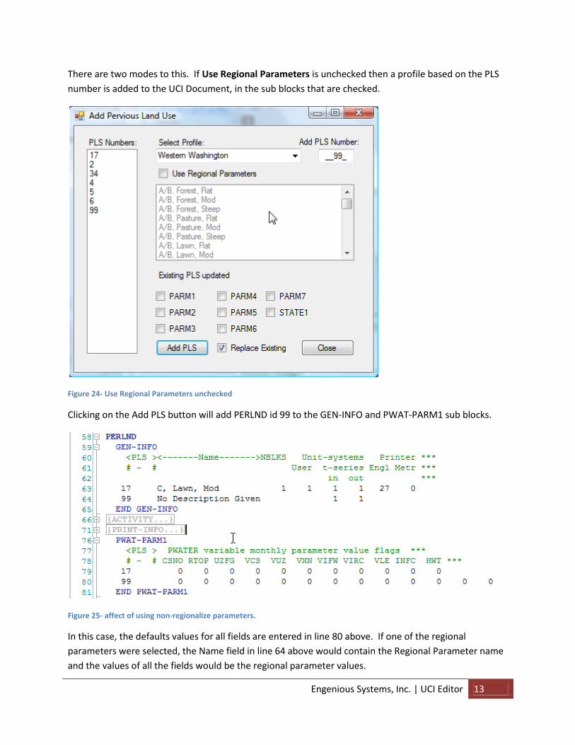
There are two modes to this. If Use Regional Parameters is unchecked then a profile based on the PLS
number is added to the UCI Document, in the sub blocks that are checked.
Figure 24- Use Regional Parameters unchecked
Clicking on the Add PLS button will add PERLND id 99 to the GEN-INFO and PWAT-PARM1 sub blocks.
Figure 25- affect of using non-regionalize parameters.
In this case, the defaults values for all fields are entered in line 80 above. If one of the regional
parameters were selected, the Name field in line 64 above would contain the Regional Parameter name
and the values of all the fields would be the regional parameter values.

14 UCI Editor | Engenious Systems, Inc.
If the sub block is not in the UCI, the sub block is added to the PERLND section.
The dialog is configured such that multiple Regional Parameters can be
selected and added at the same time. Selection of a PLS number simply
highlights the land use in the regional parameters section if it is found.
This feature is provided to remind users of the land use description
associated with a land use number.
When the Add PLS button is clicked, the selected land uses will either
be added to each of the selected sub blocks OR the Regional Parameter
or default values will replace what is currently there. If the Replace
Existing box is checked, then the Regional Parameter values will replace
the values in the UCI document, if it is unchecked, the values of the
parameters in the UCI document will remain unchanged.
Incidentally, there are two ways to access this command. Obviously, from the menu, but also when the
cursor is situated on any line within any PERLND block. Simply right mouse click, and select the Add
PERLND selection from the pop-up menu.
Add IMPLNDS
The Add IMPLND dialog box looks similar to the Add PERLND dialog box and act similarly, except that
different sub blocks are populated. There is also a pop-up menu selection for this feature.
Add MASSS-LINK
HSPF projects typically use MASS-LINK block. This feature assists in the addition of MASS-LINK
instructions and the creation of MASS-LINK blocks. There are two ways to access the command access
this command, from the menu or by right mouse clicking within the Major MASS-LINK block and
selecting the menu item.
Figure 26- Add PERLND pop up.
Engenious Systems, Inc. | UCI Editor 15
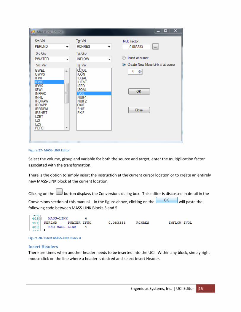
Figure 27- MASS-LINK Editor
Select the volume, group and variable for both the source and target, enter the multiplication factor
associated with the transformation.
There is the option to simply insert the instruction at the current cursor location or to create an entirely
new MASS-LINK block at the current location.
Clicking on the button displays the Conversions dialog box. This editor is discussed in detail in the
Conversions section of this manual. In the figure above, clicking on the will paste the
following code between MASS-LINK Blocks 3 and 5.
Figure 28- Insert MASS-LINK Block 4
Insert Headers
There are times when another header needs to be inserted into the UCI. Within any block, simply right
mouse click on the line where a header is desired and select Insert Header.

16 UCI Editor | Engenious Systems, Inc.
Figure 29- Insert Header
In the above example, the user right mouse clicked the cursor on line 121. Selection of the Insert
Header menu item results in:
Figure 30- Block with Inserted Header
EXT SOURCES
This utility actually does two things, it gets the starting and ending date for the precipitation time series
for the GLOBAL BLOCK, and it creates the EXT SOURCES lines for those time series. The assumption is
that the UCI document is opened and that the FILES BLOCK has a WDM file specified.

Engenious Systems, Inc. | UCI Editor 17
Figure 31-Sample FILE BLOCK for EXT SOURCES dialog
In Figure 31, lines 14 and 26 specify two (2) WDM files that are to be used with this project. Notice that
filenames do not require full and complete paths, relative paths work fine. Opening the EXT SOURCES
dialog box and selecting a WDM file and DSN will present the following:
Figure 32-EXT SOURCES dialog

18 UCI Editor | Engenious Systems, Inc.
If the is clicked, the date range is formatted and placed in the info box. If the
is checked, then the same information is placed on the clipboard, ready to paste into the
GLOBAL BLOCK, in this example, the contents of the clipboard would replace line 5.
Figure 33-GLOBAL BLOCK before pasting
Clicking on the button creates lines that can be pasted into the EXT SOURCES BLOCK.
Figure 34-Sample of EXT SOURCES lines for pasting.
The multiplier shown is a default and PROBABLY not correct. This is a value that must be determined by
the user. It is related to the physical location of the project site relative to the location of the
precipitation time series. Washington State typically computes a ratio based on the 25 year isopluvial.
We think that if that is the method for determining the multiplier, a 2 year isopluvial is more
appropriate.
Insert New Block
There are a ton of BLOCKS that are available when using HSPF. There are so many that it becomes an
issue when half way through a project, a decision is made to extend the analysis. Have a block already
defined in the UCI document goes a long way towards its usability. It is one thing to have a BLOCK
already defined and simply follow the header for input. It’s another to create the block and header from
scratch.
This tool simply inserts a block and header into the UCI document. The feature can be found in the UCI-
>ADD->Block w/Heading menu location.
Engenious Systems, Inc. | UCI Editor 19
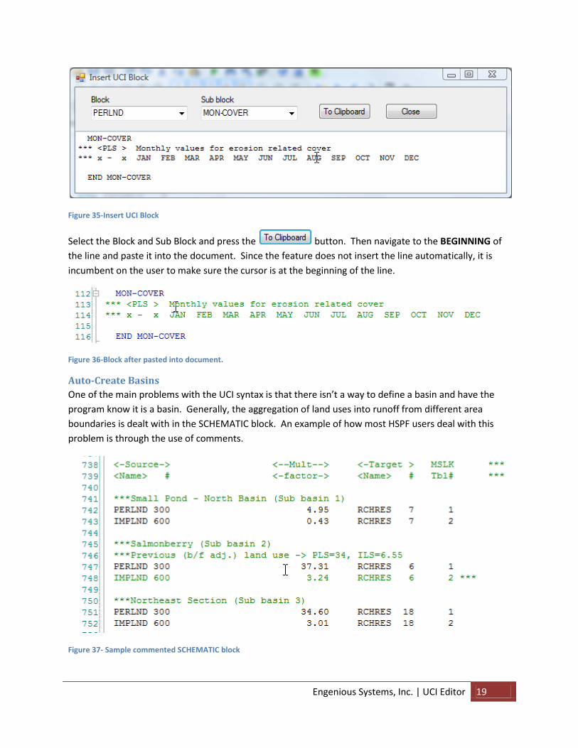
Figure 35-Insert UCI Block
Select the Block and Sub Block and press the button. Then navigate to the BEGINNING of
the line and paste it into the document. Since the feature does not insert the line automatically, it is
incumbent on the user to make sure the cursor is at the beginning of the line.
Figure 36-Block after pasted into document.
Auto-Create Basins
One of the main problems with the UCI syntax is that there isn’t a way to define a basin and have the
program know it is a basin. Generally, the aggregation of land uses into runoff from different area
boundaries is dealt with in the SCHEMATIC block. An example of how most HSPF users deal with this
problem is through the use of comments.
Figure 37- Sample commented SCHEMATIC block

20 UCI Editor | Engenious Systems, Inc.
In response to this shortcoming in the UCI syntax, HSPFToolkit has introduces a proprietary block that is
accessible to the toolkit but is really just another comment to HSPF. The format of the block is the name
of the Block followed by the basin description.
Figure 38- Example SUBBSN Block
This is a proprietary block that only the toolkit will recognize as a block. In HSPF it will be a commented
line. The Basin Description is absolutely required in line 201, with the END SUBBSN tag, not line 199
with the BLOCK command! In the collapsed form this appears as:
Figure 39- Collapsed SUBBSN block
If the Basin Description were omitted from line 201 above, the collapsed block would appear as:
Figure 40- Collapsed Block with Basin Description omitted from END tag
What can be done with existing UCI documents? Assume you have a document with the following
SCHEMATIC block:
Figure 41-SCHEMATIC Block before Auto-Create Command

Engenious Systems, Inc. | UCI Editor 21
By selecting UCI->Misc->AutoCreate Basins, the program will isolate and name the perceived basins as
follows:
Figure 42 – Auto Create Basins
While the above is fairly clean, it isn’t exactly what the engineer really had in mind. What was really
intended was for SUBBSN 1 to target both RCHRES 1 and COPY 1. The way to fix the problem is to simply
copy lines 206 through 208 and insert them at line 204. (At the time of this writing, deleting line 204
and 205 crashes the program when attempting to collapse the new block.)
Figure 43-User Modified SUBBSN tags
With the SUBBSN tags in place, HSPFToolkit can now distinguish land uses by drainage area.
SUBBSN’s must be defined in order to activate the SCHEMATIC Layout feature!
Extracting Info from UCI There are several tools available to actually extract information from the UCI document or to add hidden
information to the UCI for use in the WDM side of the program.
22 UCI Editor | Engenious Systems, Inc.
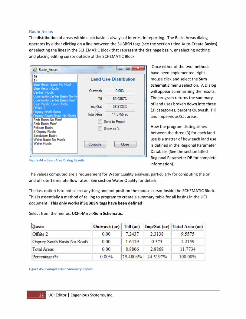
Basin Areas
The distribution of areas within each basin is always of interest in reporting. The Basin Areas dialog
operates by either clicking on a line between the SUBBSN tags (see the section titled Auto-Create Basins)
or selecting the lines in the SCHEMATIC Block that represent the drainage basin, or selecting nothing
and placing editing cursor outside of the SCHEMATIC Block.
Once either of the two methods
have been implemented, right
mouse click and select the Sum
Schematic menu selection. A Dialog
will appear summarizing the results.
The program returns the summary
of land uses broken down into three
(3) categories, percent Outwash, Till
and Impervious/Sat areas.
How the program distinguishes
between the three (3) for each land
use is a matter of how each land use
is defined in the Regional Parameter
Database (See the section titled
Regional Parameter DB for complete
information).
The values computed are a requirement for Water Quality analysis, particularly for computing the on
and off site 15 minute flow rates. See section Water Quality for details.
The last option is to not select anything and not position the mouse cursor inside the SCHEMATIC Block.
This is essentially a method of telling to program to create a summary table for all basins in the UCI
document. This only works if SUBBSN tags have been defined!
Select from the menus, UCI->Misc->Sum Schematic.
Figure 45- Example Basin Summary Report
Figure 44 – Basin Area Dialog Results.

Engenious Systems, Inc. | UCI Editor 23
DSN Descriptions
DSN Descriptions don’t do anything for the UCI document. It is really for the data side of the
HSPFToolkit program. It is important because it will help you manage the times series datasets that are
created.
The huge problem with the time series datasets is that HSPF and the UCI really only identifies them
based on their number. That is perfectly adequate for a computer, it leaves much to be desired for
people looking at and trying to make sense of the data.
HSPF takes precipitation time series and generates runoff from them, placing the resultant time series
into the WDM database. The resultant time series are identified in the database by their DSN (data set
number).
The goal of DSN Descriptions is to attach realistic names to the dataset numbers defined in the EXT
TARGETS block of the UCI document.
Figure 46- Example of EXT TARGETS Block
In the above figure, the target DSN are 1000, 1001, 701, and 801. Even though there are just four of
them, it is not clear what they represent.
Right mouse clicking anywhere within the EXT TARGETS block will present a menu. Select DSN
Assignments.
Figure 47- DSN Assignments
It repeats two columns within the EXT TARGETS block and adds two more fields. The description is
automatically generated by the program. It is nothing more than the RCHRES description found in the
GEN-INFO sub block of the RCHRES Block with source member and outlet number appended to it.
24 UCI Editor | Engenious Systems, Inc.
The RCHRES descriptions are mostly sufficient to describe what the DSN represents. It is the From COPY
1 and From COPY 501 that are the problem. The dialog allows for editing of these descriptions to
something that is more informative.
The last column (scenario) is defaulted to CURRENT. They are all listed as CURRENT because that is the
default scenario. The program really doesn’t know scenario the data set actually represents. It would
be nice to distinguish the data sets that are representative of historic, current and mitigated conditions.
HSPFToolkit really does not want users to type in their own scenario, primarily for typing reasons.
To change the scenario in the fourth column of any row, first select the scenario from the
drop down, then just click on the scenario field in the table.
If you insist on creating a custom scenario, they you will have to deal with the typing yourself. Click in
the scenario field in the table and edit the text.
The checkbox provides the option of either cleaning up the
database to only contain DSN numbers in the current EXT TARGETS block of the UCI document or leaving
DSN numbers in the database that were defined in other UCI documents that use the same WDM
database.
Most of the time, if there is only one UCI document associated with the HSPF WDM database, it is ok to
check this box. If, on the other hand, there is a UCI document that generated DSN numbers for the
historic condition and another that generates DSN numbers for the mitigated condition, then this should
be left unchecked.
The value of these DSN Assignments will be evident when dealing with the WDM portion of HSPFToolkit.
Compare w/DB
There are so many possible permutations of the PERLND and IMPLND land uses that it is sometimes
difficult to know whether the combination of values represent the land use description. Assuming that a
project has created all the land uses with the values found in the Regional Parameters database
(discussed in Section Regional Parameter DB), this feature will compare the values for each land use
with the values in the Regional Parameter database.
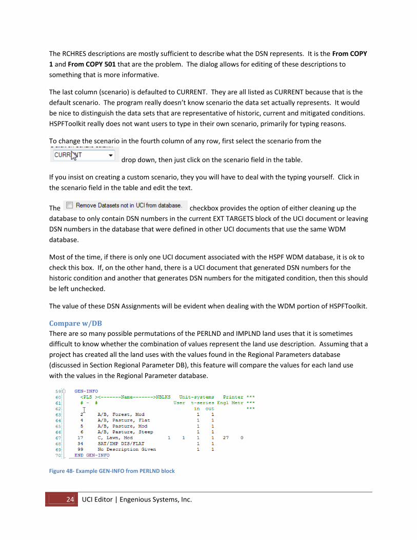
Figure 48- Example GEN-INFO from PERLND block
Engenious Systems, Inc. | UCI Editor 25
The above figure shows the different land uses found in our example UCI document. It has been
changed and modified throughout the writing of the document. To find out how it compares with the
Regional Parameter database, simply select UCI->Add->Compare w/DB.
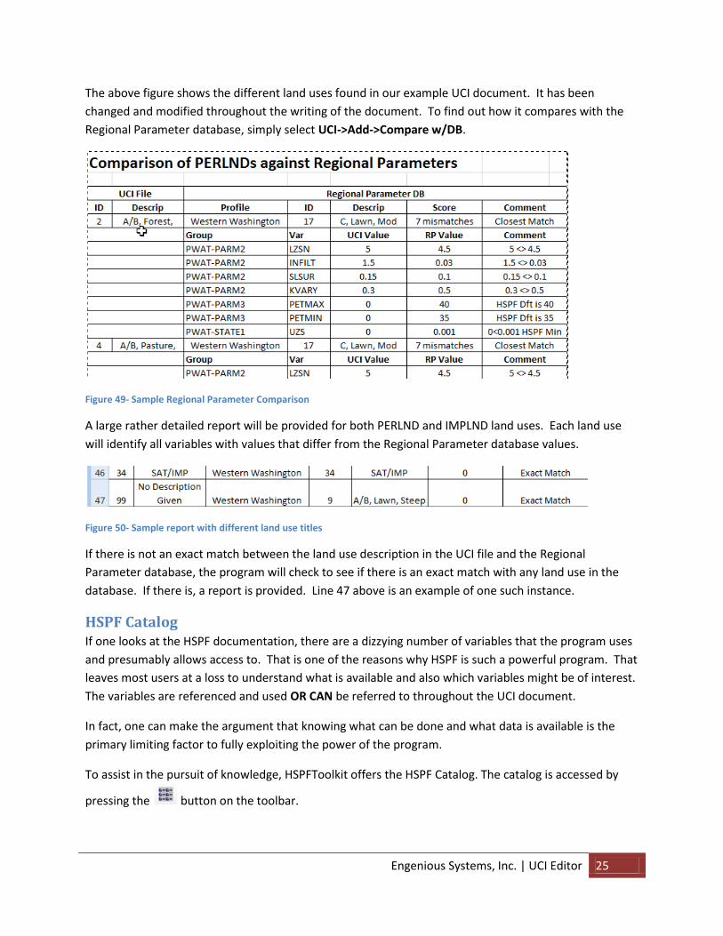
Figure 49- Sample Regional Parameter Comparison
A large rather detailed report will be provided for both PERLND and IMPLND land uses. Each land use
will identify all variables with values that differ from the Regional Parameter database values.
Figure 50- Sample report with different land use titles
If there is not an exact match between the land use description in the UCI file and the Regional
Parameter database, the program will check to see if there is an exact match with any land use in the
database. If there is, a report is provided. Line 47 above is an example of one such instance.
HSPF Catalog If one looks at the HSPF documentation, there are a dizzying number of variables that the program uses
and presumably allows access to. That is one of the reasons why HSPF is such a powerful program. That
leaves most users at a loss to understand what is available and also which variables might be of interest.
The variables are referenced and used OR CAN be referred to throughout the UCI document.
In fact, one can make the argument that knowing what can be done and what data is available is the
primary limiting factor to fully exploiting the power of the program.
To assist in the pursuit of knowledge, HSPFToolkit offers the HSPF Catalog. The catalog is accessed by
pressing the button on the toolbar.
26 UCI Editor | Engenious Systems, Inc.
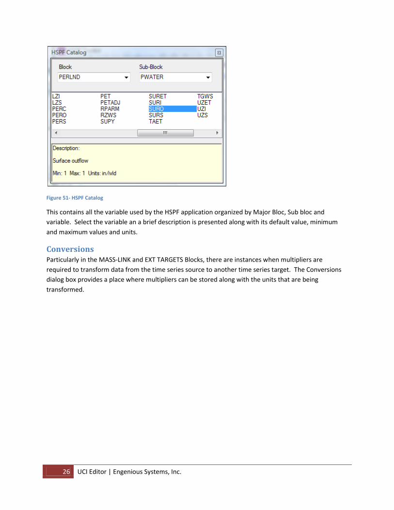
Figure 51- HSPF Catalog
This contains all the variable used by the HSPF application organized by Major Bloc, Sub bloc and
variable. Select the variable an a brief description is presented along with its default value, minimum
and maximum values and units.
Conversions Particularly in the MASS-LINK and EXT TARGETS Blocks, there are instances when multipliers are
required to transform data from the time series source to another time series target. The Conversions
dialog box provides a place where multipliers can be stored along with the units that are being
transformed.
Engenious Systems, Inc. | UCI Editor 27
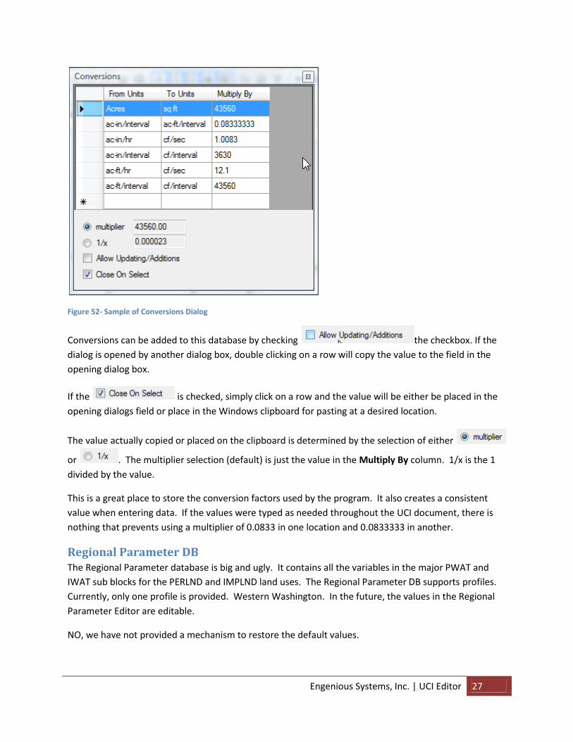
Figure 52- Sample of Conversions Dialog
Conversions can be added to this database by checking the checkbox. If the
dialog is opened by another dialog box, double clicking on a row will copy the value to the field in the
opening dialog box.
If the is checked, simply click on a row and the value will be either be placed in the
opening dialogs field or place in the Windows clipboard for pasting at a desired location.
The value actually copied or placed on the clipboard is determined by the selection of either
or . The multiplier selection (default) is just the value in the Multiply By column. 1/x is the 1
divided by the value.
This is a great place to store the conversion factors used by the program. It also creates a consistent
value when entering data. If the values were typed as needed throughout the UCI document, there is
nothing that prevents using a multiplier of 0.0833 in one location and 0.0833333 in another.
Regional Parameter DB The Regional Parameter database is big and ugly. It contains all the variables in the major PWAT and
IWAT sub blocks for the PERLND and IMPLND land uses. The Regional Parameter DB supports profiles.
Currently, only one profile is provided. Western Washington. In the future, the values in the Regional
Parameter Editor are editable.
NO, we have not provided a mechanism to restore the default values.
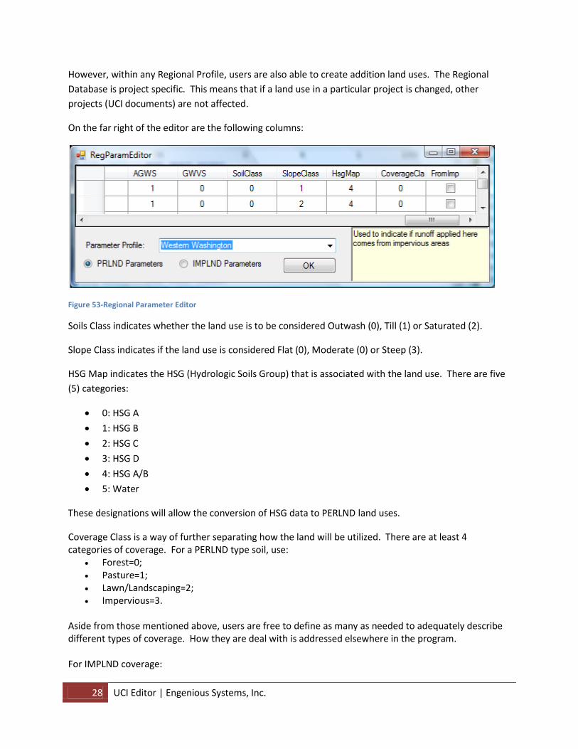
28 UCI Editor | Engenious Systems, Inc.
However, within any Regional Profile, users are also able to create addition land uses. The Regional
Database is project specific. This means that if a land use in a particular project is changed, other
projects (UCI documents) are not affected.
On the far right of the editor are the following columns:
Figure 53-Regional Parameter Editor
Soils Class indicates whether the land use is to be considered Outwash (0), Till (1) or Saturated (2).
Slope Class indicates if the land use is considered Flat (0), Moderate (0) or Steep (3).
HSG Map indicates the HSG (Hydrologic Soils Group) that is associated with the land use. There are five
(5) categories:
0: HSG A
1: HSG B
2: HSG C
3: HSG D
4: HSG A/B
5: Water
These designations will allow the conversion of HSG data to PERLND land uses.
Coverage Class is a way of further separating how the land will be utilized. There are at least 4 categories of coverage. For a PERLND type soil, use:
Forest=0; Pasture=1; Lawn/Landscaping=2; Impervious=3.
Aside from those mentioned above, users are free to define as many as needed to adequately describe different types of coverage. How they are deal with is addressed elsewhere in the program. For IMPLND coverage:

Engenious Systems, Inc. | UCI Editor 29
Roads=0; Rooftop=1; Driveways=2; Sidewalk=3; Parking=4; Ponds=5.
UCI Specs Our HSPF database of commands is very extensive. There is always the possibility that something isn’t
right in the database. The UCI spec is to make changes to values that the program depends on to find
variables, set defaults, position variables on lines, etc. If something doesn’t work, call us, we will figure
it out and tell you how to fix it.
This feature is turned off until we need to turn it on for you.
FTABLES If there is anything to HSPF, it is their FTABLES. FTABLES are the meat and potatoes of the program.
FTABLES are used for all physical transformations of time series through physical (real world) structures.
To HSPF, FTABLES are just rating curve tables. There is no assistance by the HSPF application in
developing the rating curves that are necessary for any type of analysis.
FTABLES are either lakes, reaches (channels) or wetlands. Lakes are the interesting part of the FTABLE,
lakes are detention structures with complex outlets.
The last time we looked, HSPF imposed a limit on the number of lines supported by the
FTABLE (90 lines). The FTABLES that this program creates are not limited to 90 lines. Unlike
some programs that will create an FTABLE to utilize all 90 lines, this program leaves it to the
user to enforce the requirement. The interval for all FTABLES can be set at the tool. Use
engineering judgment when creating FTABLES!
Lakes
A Lake is a stage-storage rating curve with an overflow weir. There are lots of ways to generate them.
HSPFToolkit offers a pond sizing dialog. Discussion on how to size ponds will be provided elsewhere.
Here we intend to discuss creation of FTABLES for lakes and detention structures.
In order to access the Pond Design Dialog, a WDM database file must be opened. Select WDM Utils-
>Open WDM from the menu and open a WDM database file.
To open the Pond Sizing Worksheet, select UCI->ADD->Pond Sizing.

30 UCI Editor | Engenious Systems, Inc.
Figure 54- Pond Sizing Dialog
There is lot to this dialog. What we are focusing on are the Storage and Discharge tabs in the lower left
and the button. This dialog allows for the independent specification of a Storage Curve
and Discharge Curve. Once defined the button can be select to display the FTABLE in the
large area on the right.
There is the option of Verbose, which means to provide all the data in the form of comments that was
used to create the FTABLE and All Outlets, which tells the program to provide a column for each
discharge structure instead of combining them all into one discharge rating curve. When the FTABLE is
satisfactory, it will be placed on the clipboard, ready to paste into the UCI document.

Engenious Systems, Inc. | UCI Editor 31
Figure 55-Sample of FTABLE generated by Pond Sizing Worksheet
Assuming that we have created an FTABLE and placed it on the Clipboard, simply navigate to the proper
location in the UCI document and paste it in. It is fully formed in memory and needs no modification or
adjustment prior to pasting.
The use of the Pond Sizing worksheet is closely linked to the FTABLES, which are closely linked to the
RCHRES. There is a one-one correlation and if an FTABLE is created, it has to be associated with a
RCHRES.
Storage
Choices of storage elements that make up an FTABLE are:
Trapezoidal shaped ponds
Vaults
Circular Tanks
Arch Tanks
Depth-Area rating curves
Sand Filters
Gravel Trench
With the exception of Sand Filter and Gravel Trench, all storage structures can have a void ratio applied
to the volume that is computed. Obviously, a void ratio of one (1) means 100% voids. Generally, the
bottom elevation is left at zero. HSPF doesn’t care what about absolute elevations of its hydraulic
objects.
For Trapezoidal and Vault structures, there is a specification for maximum depth. This controls the
maximum elevation of the rating curve that is created.
The Depth-Area is a really a Depth-Area-Volume table. We don’t think anyone would want to enter a
table manually. The implementation of this is to create three columns in EXCEL.

32 UCI Editor | Engenious Systems, Inc.
Column 1 is the stage (ft)
Column 2 is the area (acres)
Column3 is the volume (ac-ft)
Select the columns and rows that contain the numbers, copy to the clipboard. Right mouse click in the
data grid and select paste from clipboard.
The Sand Filter and Gravel Trench are special structures. They are included in this location because we
are too lazy to repeat much of the underlying programming to generate the FTABLES. Both of these are
for the purpose of generating FTABLES. However, neither is suitable for use as a detention structure for
pond sizing.
Sand Filters
A Sand Filter is a structure that filters water runoff through it to affect some level of treatment.
Physically, is shaped as either a trapezoidal or vault type structure with a layer of sand at the bottom.
From the standpoint of this program, it requires two Storage tabs to be completed. The first is the Trap
Tab.
Figure 56- Sand Filter Example
In this case we have a storage container that is 7 ft deep that is 100 x 100 ft with 3:1 side slopes. The
second tab that needs to be identified (filled out) is the Sand Filter tab.
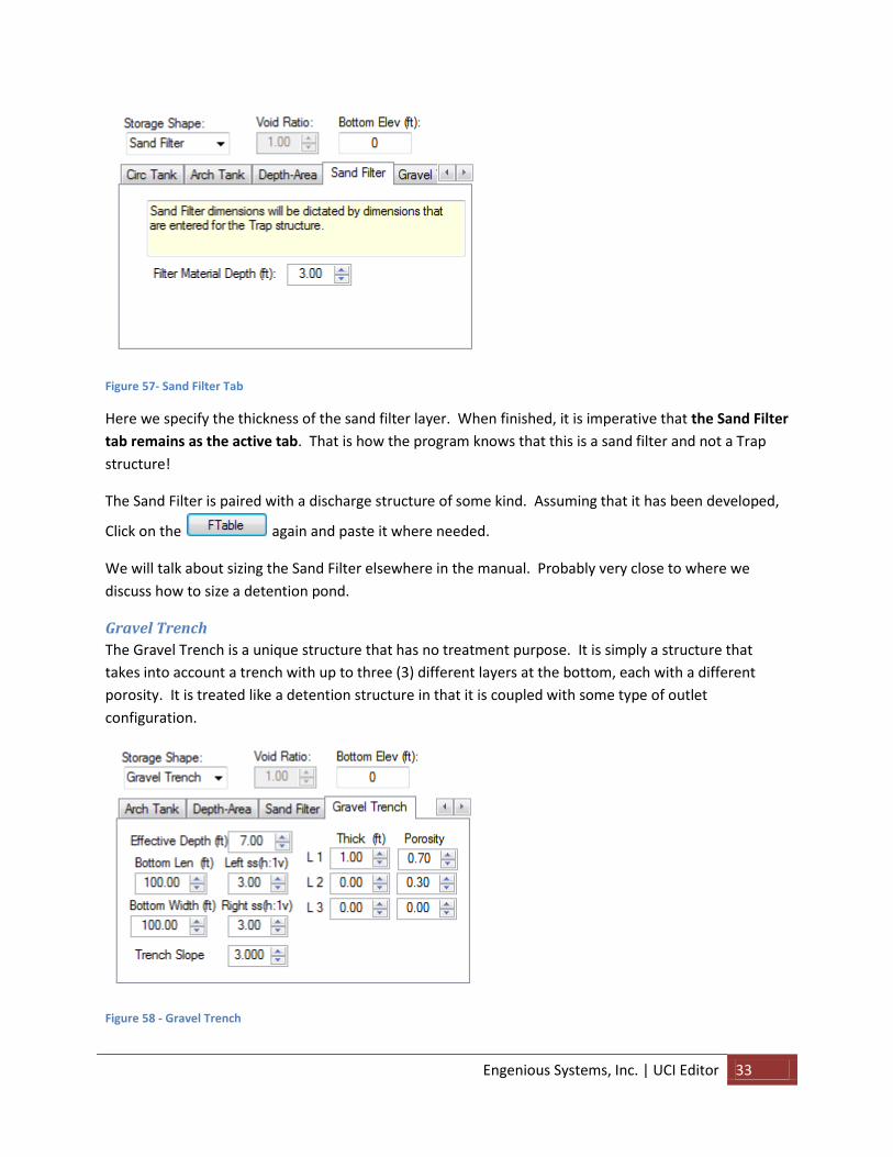
Engenious Systems, Inc. | UCI Editor 33
Figure 57- Sand Filter Tab
Here we specify the thickness of the sand filter layer. When finished, it is imperative that the Sand Filter
tab remains as the active tab. That is how the program knows that this is a sand filter and not a Trap
structure!
The Sand Filter is paired with a discharge structure of some kind. Assuming that it has been developed,
Click on the again and paste it where needed.
We will talk about sizing the Sand Filter elsewhere in the manual. Probably very close to where we
discuss how to size a detention pond.
Gravel Trench
The Gravel Trench is a unique structure that has no treatment purpose. It is simply a structure that
takes into account a trench with up to three (3) different layers at the bottom, each with a different
porosity. It is treated like a detention structure in that it is coupled with some type of outlet
configuration.
Figure 58 - Gravel Trench

34 UCI Editor | Engenious Systems, Inc.
The storage rating curve takes into account the thickness of the layers and porosity. It is a fairly simple
rating curve because the assumption is that the trench is flat, or rather the depth in the trench is parallel
to the layers.
Discharge Controls
HSPFToolkit offers a single Discharge Control that pairs with the Storage controls. Within the single
control is the ability to define a combination discharge rating curve consisting of:
Infiltration
Up to three orifice at situated at different depths
A weir that can be defined as either a rectangular, vee or sutro weir
An overflow riser
Infiltration can be applied to the wetted bottom or the surface area. It can be a straight infiltration rate
or a Ksat (saturated hydraulic conductivity) value. Infiltration is applied based on Darcy’s equation and
will vary with depth. If a Ksat value is used, it is supported by a Ksat entry or a soil log table.
If the Ksat option is selected, there is the option of
specifying High Potential for Bio-fouling and an average to
high degree of long term maintenance/performance
monitoring. These options are documented in the
Washington State Department of Ecology design manual.
The benefit of a soil log table is that Ksat values are
computed based on elevation from the bottom of the pond.
Infiltration rates can also have a safety factor applied to
them.
If the is unchecked, there is the option of specifying either theThirsty Duck discharge
structure or a custom stage-discharge table.
FTABLE Lookup
Occasionally when looking at a UCI document, there is an interest in either getting a flow rate that
corresponds to a stage or a stage that corresponds to a flow rate. Select UCI->FTABLE->Lookup.
Figure 59 - Ksat option of Infiltration

Engenious Systems, Inc. | UCI Editor 35
Figure 60- Sample FTABLE Lookup
This is actually a pretty neat tool. When the dialog opens, the program remembers the last FTABLE that
was selected or it will default to the first one. It has already looked at the FTABLE and shows the range
of values for the stage and flows.
There are two options. Either enter a stage and look up the flow or enter a flow and look up the stage.
It really isn’t meant to produce a report, however the answer is sent to the second tab (the tab that
displays the WDM information) for a cut and paste if needed.
FTABLE Define Section
HSPF was originally designed or big flows. In general, a RCHRES is a channel of some shape that conveys
runoff from point A to point B. If the FTABLE isn’t a lake, it is most likely a channel.

36 UCI Editor | Engenious Systems, Inc.
Figure 61- Channel Section
The Channel Worksheet allows for the definition of a left bank, center channel and right overflow bank.
Each section can have a different Manning’s roughness coefficient. Only the center can have a flat
bottom. The left and right overflow bank must have a slope towards the center.
It is possible to apply an infiltration rate to the channel. The infiltration rate is applied as a constant rate
based on the length and slope of the channel.
To assist in the Manning’s numbers, mouse clicking in the
Manning’s n field will display a pop up
Like other FTABLE tools, the FTABLE does not automatically
replace the FTABLE in the UCI document. Instead, it is placed In
the clipboard and can then be pasted.
The table presents the user with a choice between Lined Channels,
Earth Channels, and natural stream manning’s numbers. Since
many of the choices represent a range of values, the program will
insert the average value for the selected choice. Figure 62-Manning's Number selection
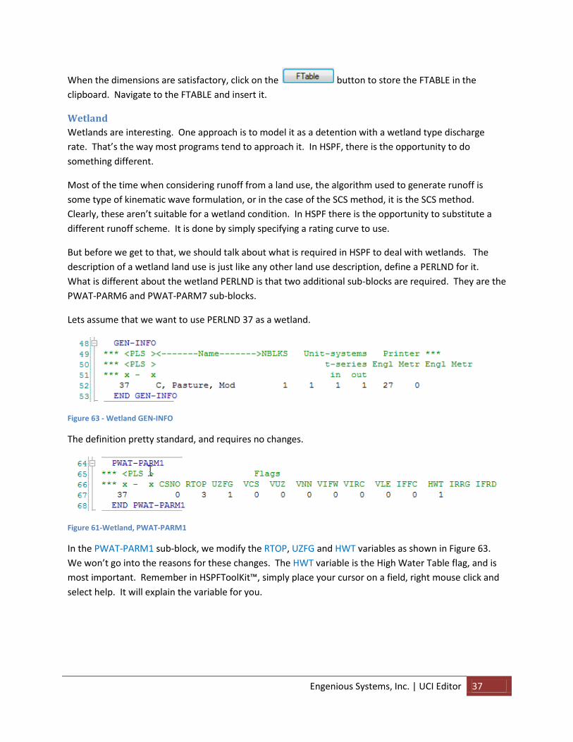
Engenious Systems, Inc. | UCI Editor 37
When the dimensions are satisfactory, click on the button to store the FTABLE in the
clipboard. Navigate to the FTABLE and insert it.
Wetland
Wetlands are interesting. One approach is to model it as a detention with a wetland type discharge
rate. That’s the way most programs tend to approach it. In HSPF, there is the opportunity to do
something different.
Most of the time when considering runoff from a land use, the algorithm used to generate runoff is
some type of kinematic wave formulation, or in the case of the SCS method, it is the SCS method.
Clearly, these aren’t suitable for a wetland condition. In HSPF there is the opportunity to substitute a
different runoff scheme. It is done by simply specifying a rating curve to use.
But before we get to that, we should talk about what is required in HSPF to deal with wetlands. The
description of a wetland land use is just like any other land use description, define a PERLND for it.
What is different about the wetland PERLND is that two additional sub-blocks are required. They are the
PWAT-PARM6 and PWAT-PARM7 sub-blocks.
Lets assume that we want to use PERLND 37 as a wetland.
Figure 63 - Wetland GEN-INFO
The definition pretty standard, and requires no changes.
Figure 61-Wetland, PWAT-PARM1
In the PWAT-PARM1 sub-block, we modify the RTOP, UZFG and HWT variables as shown in Figure 63.
We won’t go into the reasons for these changes. The HWT variable is the High Water Table flag, and is
most important. Remember in HSPFToolKit™, simply place your cursor on a field, right mouse click and
select help. It will explain the variable for you.
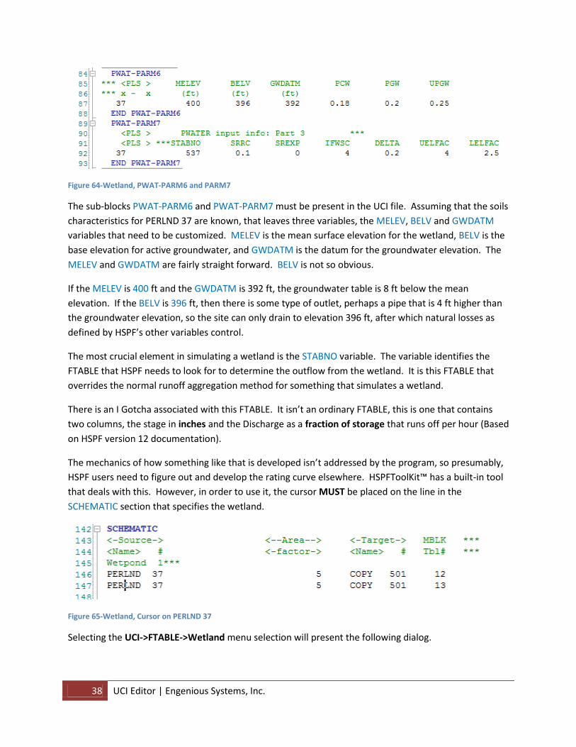
38 UCI Editor | Engenious Systems, Inc.
Figure 64-Wetland, PWAT-PARM6 and PARM7
The sub-blocks PWAT-PARM6 and PWAT-PARM7 must be present in the UCI file. Assuming that the soils
characteristics for PERLND 37 are known, that leaves three variables, the MELEV, BELV and GWDATM
variables that need to be customized. MELEV is the mean surface elevation for the wetland, BELV is the
base elevation for active groundwater, and GWDATM is the datum for the groundwater elevation. The
MELEV and GWDATM are fairly straight forward. BELV is not so obvious.
If the MELEV is 400 ft and the GWDATM is 392 ft, the groundwater table is 8 ft below the mean
elevation. If the BELV is 396 ft, then there is some type of outlet, perhaps a pipe that is 4 ft higher than
the groundwater elevation, so the site can only drain to elevation 396 ft, after which natural losses as
defined by HSPF’s other variables control.
The most crucial element in simulating a wetland is the STABNO variable. The variable identifies the
FTABLE that HSPF needs to look for to determine the outflow from the wetland. It is this FTABLE that
overrides the normal runoff aggregation method for something that simulates a wetland.
There is an I Gotcha associated with this FTABLE. It isn’t an ordinary FTABLE, this is one that contains
two columns, the stage in inches and the Discharge as a fraction of storage that runs off per hour (Based
on HSPF version 12 documentation).
The mechanics of how something like that is developed isn’t addressed by the program, so presumably,
HSPF users need to figure out and develop the rating curve elsewhere. HSPFToolKit™ has a built-in tool
that deals with this. However, in order to use it, the cursor MUST be placed on the line in the
SCHEMATIC section that specifies the wetland.
Figure 65-Wetland, Cursor on PERLND 37
Selecting the UCI->FTABLE->Wetland menu selection will present the following dialog.
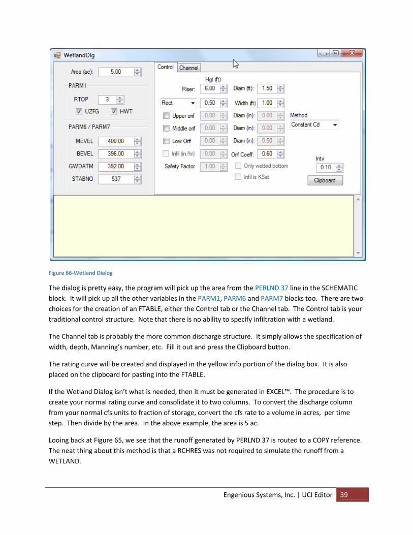
Engenious Systems, Inc. | UCI Editor 39
Figure 66-Wetland Dialog
The dialog is pretty easy, the program will pick up the area from the PERLND 37 line in the SCHEMATIC
block. It will pick up all the other variables in the PARM1, PARM6 and PARM7 blocks too. There are two
choices for the creation of an FTABLE, either the Control tab or the Channel tab. The Control tab is your
traditional control structure. Note that there is no ability to specify infiltration with a wetland.
The Channel tab is probably the more common discharge structure. It simply allows the specification of
width, depth, Manning’s number, etc. Fill it out and press the Clipboard button.
The rating curve will be created and displayed in the yellow info portion of the dialog box. It is also
placed on the clipboard for pasting into the FTABLE.
If the Wetland Dialog isn’t what is needed, then it must be generated in EXCEL™. The procedure is to
create your normal rating curve and consolidate it to two columns. To convert the discharge column
from your normal cfs units to fraction of storage, convert the cfs rate to a volume in acres, per time
step. Then divide by the area. In the above example, the area is 5 ac.
Looing back at Figure 65, we see that the runoff generated by PERLND 37 is routed to a COPY reference.
The neat thing about this method is that a RCHRES was not required to simulate the runoff from a
WETLAND.

40 UCI Editor | Engenious Systems, Inc.
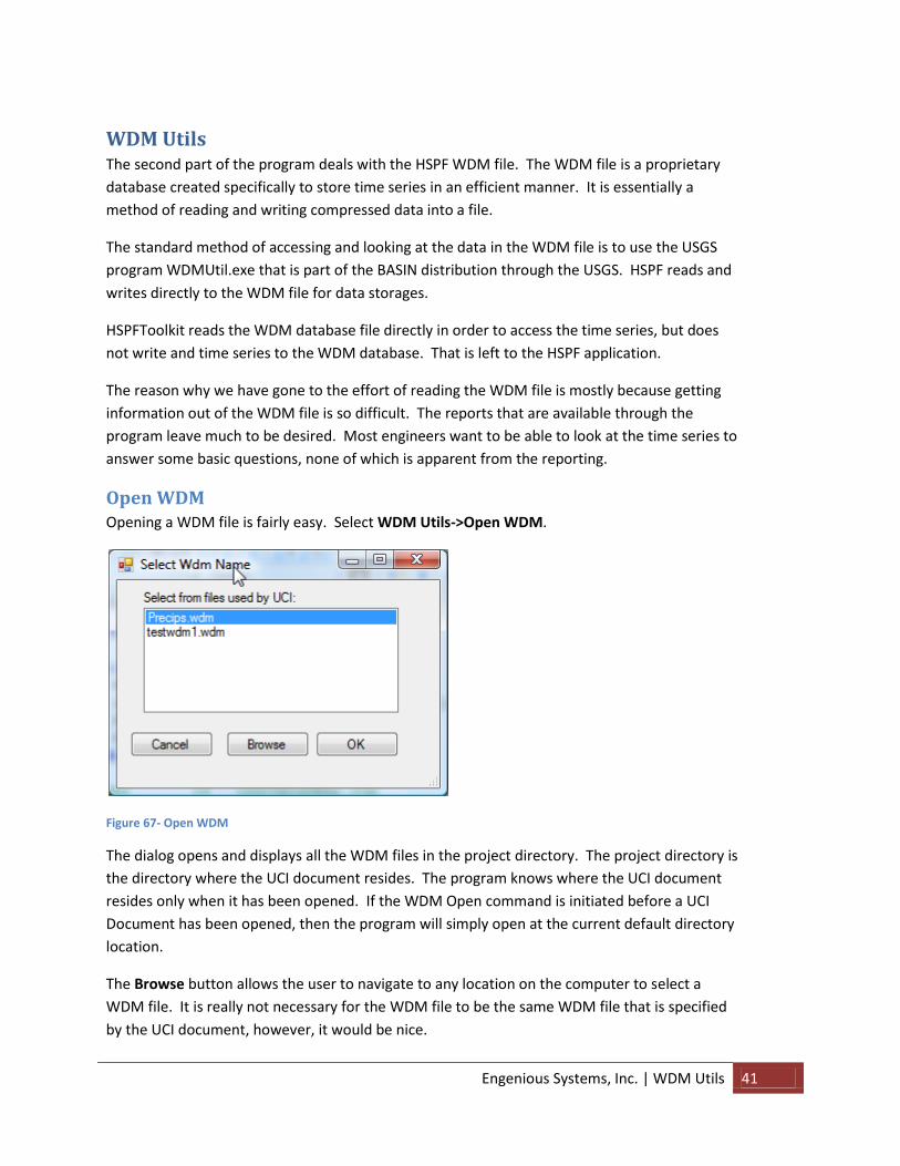
Engenious Systems, Inc. | WDM Utils 41
WDM Utils The second part of the program deals with the HSPF WDM file. The WDM file is a proprietary
database created specifically to store time series in an efficient manner. It is essentially a
method of reading and writing compressed data into a file.
The standard method of accessing and looking at the data in the WDM file is to use the USGS
program WDMUtil.exe that is part of the BASIN distribution through the USGS. HSPF reads and
writes directly to the WDM file for data storages.
HSPFToolkit reads the WDM database file directly in order to access the time series, but does
not write and time series to the WDM database. That is left to the HSPF application.
The reason why we have gone to the effort of reading the WDM file is mostly because getting
information out of the WDM file is so difficult. The reports that are available through the
program leave much to be desired. Most engineers want to be able to look at the time series to
answer some basic questions, none of which is apparent from the reporting.
Open WDM Opening a WDM file is fairly easy. Select WDM Utils->Open WDM.
Figure 67- Open WDM
The dialog opens and displays all the WDM files in the project directory. The project directory is
the directory where the UCI document resides. The program knows where the UCI document
resides only when it has been opened. If the WDM Open command is initiated before a UCI
Document has been opened, then the program will simply open at the current default directory
location.
The Browse button allows the user to navigate to any location on the computer to select a
WDM file. It is really not necessary for the WDM file to be the same WDM file that is specified
by the UCI document, however, it would be nice.

42 WDM Utils | Engenious Systems, Inc.
Close WDM Closing the WDM file is not absolutely necessary before opening another WDM. Since only one
WDM file can be accessed at a time, if one is currently opened, it will be closed.
Overview When a WDM database is opened, the user is presented with a navigation display consisting of a
list of all DSN (data set numbers) in the WDM database and a report view.
Figure 68- WDM Display
The report view contains a summary of the DSN number within the database. There are
essentially two summary tables. The first is a list of the number of datasets for each particular
type of data set. The WDM file actually supports more than just Time Series data sets. The
second is a detailed look at each DSN, listing the type, start and end date and time and the
station name.
Figure 69= Data Set Summary
All statistical functions are accessible from the Toolbar, See the Appendix for their descriptions.
Statistics When dealing with times series recurrence intervals are important. HSPFToolkit supports return
frequency analysis by rate and volume. Rate is the more traditional approach to runoff time
series analysis, volume is perhaps more informative.

Engenious Systems, Inc. | WDM Utils 43
All the statistical tools operate based on the selected DSN in the left view. In some cases,
multiple DSNs can be selected to generate a tabular report. Where multiple DSN selection is not
appropriate, only the first selected DSN will be reported.
Rate
The first set of found on the toolbar are related to runoff rate.
Summary
Clicking on any DSN will display a list of Attributes associated with the data set. HSPF only
requires TSTYPE, TCODE, TSBYR, TSSTEP, TGROUP, STANAM, TSFORM and VBTME. These
determine how data is stored and recovered from the WDM database.
The attributes are list to provide the user with insight into the information stored by the HSPF
application.
Log Pearson Frequency
Once a DSN has been selected, the button generates a Log Pearson Type III analysis on the
time series. A plot is presented for report purposes.
Figure 70- Sample Log Pearson Plot
There is the ability to save the plot to a file built into the frame of the plot. There is the option
to NOT automatically display the plot. It is found in the Misc->Preferences->Misc Options menu
sequence.
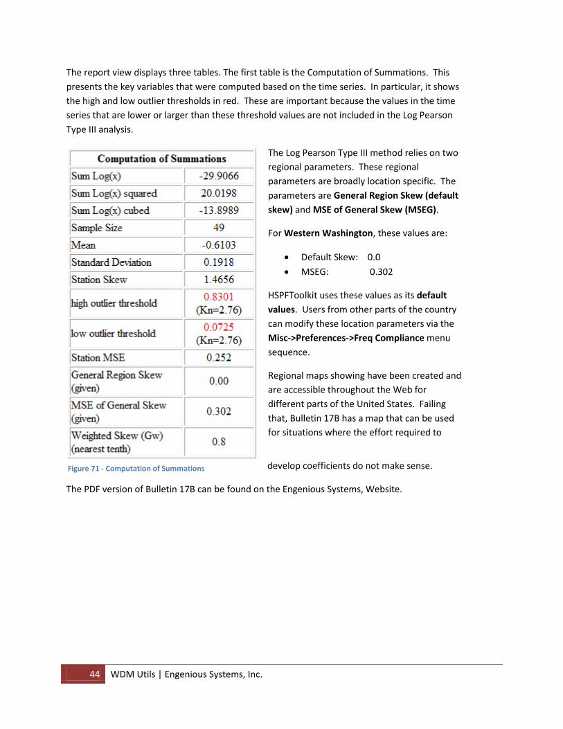
44 WDM Utils | Engenious Systems, Inc.
The report view displays three tables. The first table is the Computation of Summations. This
presents the key variables that were computed based on the time series. In particular, it shows
the high and low outlier thresholds in red. These are important because the values in the time
series that are lower or larger than these threshold values are not included in the Log Pearson
Type III analysis.
The Log Pearson Type III method relies on two
regional parameters. These regional
parameters are broadly location specific. The
parameters are General Region Skew (default
skew) and MSE of General Skew (MSEG).
For Western Washington, these values are:
Default Skew: 0.0
MSEG: 0.302
HSPFToolkit uses these values as its default
values. Users from other parts of the country
can modify these location parameters via the
Misc->Preferences->Freq Compliance menu
sequence.
Regional maps showing have been created and
are accessible throughout the Web for
different parts of the United States. Failing
that, Bulletin 17B has a map that can be used
for situations where the effort required to
develop coefficients do not make sense.
The PDF version of Bulletin 17B can be found on the Engenious Systems, Website.
Figure 71 - Computation of Summations

Engenious Systems, Inc. | WDM Utils 45
Figure 72 - Log Pearson Type III Return Frequencies
The last table presented is the confidence limits. Mostly, it is just the above table that everyone
pays attention to, however, the information present in this report seeks to draw attention to the
quality of data used in the computations.
Figure 73 - Log Pearson Confidence limits.
This table along is really more important that the actual return frequency table. Given that
these computations are based on a limited number of data point, it is not reasonable to treat a
given return frequency as absolute. Instead, it is better to understand that with each return
frequency, there is a confidence interval. This is a 95% confidence interval.
Although Figure 72 indicates that the 100 year return frequency is 0.88 cfs, Figure 73 tells
indicates that values between 0.71 and 1.2 cfs have a 95% probability that they are also 100

46 WDM Utils | Engenious Systems, Inc.
year events. Looking at Figure 70, it is easy to see that there were no data point used in the
computation that met the 100 year return frequency level. In fact, there was only one at the 50
year level.
Peak Years
Selection of the button on the toolbar presents a Pear Yearly flow rate report. This report
will recognize the selection of multiple DSN numbers. It provides a table for comparison.
Figure 74 - Sample Peak Yearly Flow Report
These values are the values used to generate the Log-Pearson Type III Analysis.
Ranked Peak Years
Selection of the button presents a Ranked Peak Yearly report. Since the report is ranked,
only one DSN can be ranked at a time.
Figure 75 - Ranked Peak Yearly Report
The primary purpose for ranking is to see when the peak year occurred. In this case it was the
1996-1997 water year. Looking at Figure 70, it was probably a 50 year event.

Engenious Systems, Inc. | WDM Utils 47
Return Years
Selection of the button presents a Return Rate report. Basically, it is a report that identifies
the water year that most closely matches the computed return frequency rate.
Figure 76 - Years Closest to Return Frequency Rate
Plotting Position
Selection of the button returns return frequencies based on plot positioning. There are
numerous positioning algorithms, the default is Gringorton. This report provides both the
return frequency and the ranking.
In this example, the Gringorton 50 year rate is 0.8625 cfs, while the Log Pearson 100 year rate is
0.8796 cfs. Different method, different answer.
HSPFToolkit also supports the Cunnane, Gumbel, Log Normal, and Weibull plot positioning.
These options are available in the Misc->Preferences->Misc Options menu selection.

48 WDM Utils | Engenious Systems, Inc.
Figure 77 - Gringorton Plotting Positioning
Unlike Log Pearson, a return frequency is not returned if there is insufficient data.
Export Frequencies to StormShed3G™
This feature automatically export the design frequencies compute by HSPF to a StormShed3G
project. Select WDM Utils->Statistics By Rate->Export Freq menu sequence.
Figure 78- Export Return Frequencies to StormShed3G
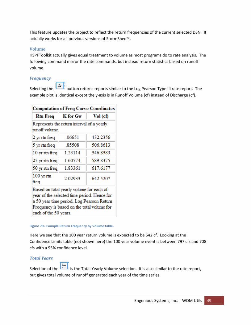
Engenious Systems, Inc. | WDM Utils 49
This feature updates the project to reflect the return frequencies of the current selected DSN. It
actually works for all previous versions of StormShed™.
Volume
HSPFToolkit actually gives equal treatment to volume as most programs do to rate analysis. The
following command mirror the rate commands, but instead return statistics based on runoff
volume.
Frequency
Selecting the button returns reports similar to the Log Pearson Type III rate report. The
example plot is identical except the y-axis is in Runoff Volume (cf) instead of Discharge (cf).
Figure 79- Example Return Frequency by Volume table.
Here we see that the 100 year return volume is expected to be 642 cf. Looking at the
Confidence Limits table (not shown here) the 100 year volume event is between 797 cfs and 708
cfs with a 95% confidence level.
Total Years
Selection of the is the Total Yearly Volume selection. It is also similar to the rate report,
but gives total volume of runoff generated each year of the time series.
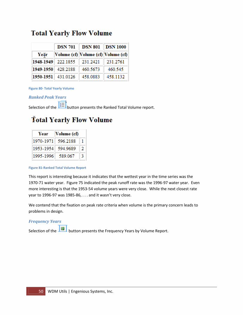
50 WDM Utils | Engenious Systems, Inc.
Figure 80- Total Yearly Volume
Ranked Peak Years
Selection of the button presents the Ranked Total Volume report.
Figure 81-Ranked Total Volume Report
This report is interesting because it indicates that the wettest year in the time series was the
1970-71 water year. Figure 75 indicated the peak runoff rate was the 1996-97 water year. Even
more interesting is that the 1953-54 volume years were very close. While the next closest rate
year to 1996-97 was 1985-86, . . . and it wasn’t very close.
We contend that the fixation on peak rate criteria when volume is the primary concern leads to
problems in design.
Frequency Years
Selection of the button presents the Frequency Years by Volume Report.
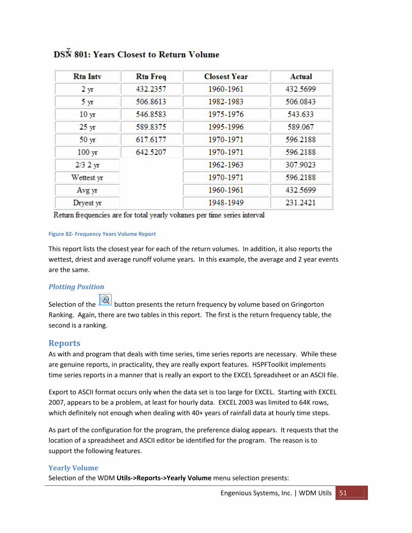
Engenious Systems, Inc. | WDM Utils 51
Figure 82- Frequency Years Volume Report
This report lists the closest year for each of the return volumes. In addition, it also reports the
wettest, driest and average runoff volume years. In this example, the average and 2 year events
are the same.
Plotting Position
Selection of the button presents the return frequency by volume based on Gringorton
Ranking. Again, there are two tables in this report. The first is the return frequency table, the
second is a ranking.
Reports As with and program that deals with time series, time series reports are necessary. While these
are genuine reports, in practicality, they are really export features. HSPFToolkit implements
time series reports in a manner that is really an export to the EXCEL Spreadsheet or an ASCII file.
Export to ASCII format occurs only when the data set is too large for EXCEL. Starting with EXCEL
2007, appears to be a problem, at least for hourly data. EXCEL 2003 was limited to 64K rows,
which definitely not enough when dealing with 40+ years of rainfall data at hourly time steps.
As part of the configuration for the program, the preference dialog appears. It requests that the
location of a spreadsheet and ASCII editor be identified for the program. The reason is to
support the following features.
Yearly Volume
Selection of the WDM Utils->Reports->Yearly Volume menu selection presents:

52 WDM Utils | Engenious Systems, Inc.
Figure 83- Peak Yearly Volume Report
This report appears in the WDM View window. It summarizes peak yearly rates, average
monthly volume, and total yearly volume. All reports in the WDM View window can be cut and
paste directly into EXCEL or Microsoft Word.
Monthly Volume
Selection of the WDM Utils->Reports->Monthly Volume menu selection presents:
Figure 84- Monthly Volume Report
Similar to the Yearly volume report, except on a monthly basis.
Daily Rate
Selection of the WDM Utils->Reports->Daily Rate menu selection:

Engenious Systems, Inc. | WDM Utils 53
Figure 85- Excel Report of Daily Rate
This report should open in EXCEL, even at 50 years worth of data, it amounts to about 19K rows
of data at one row per day, well within the capabilities of EXCEL.
Hourly Rate
Selection of the WDM Utils->Reports->Hourly Rate menu selection:
Figure 86- Hourly Rate data in EXCEL
In EXCEL 2007 can handle the large amount of hourly data. If EXCEL 2007 is not available, the
program will resort to the ASCII editor. A file will be created in the project directory (where the
UCI file is located) with the UCI name and the .csv filename extension.
Figure 87- ASCII File format for hourly rates.

54 WDM Utils | Engenious Systems, Inc.
In the case of the current example, if the name of the UCI document is MYProject.UCI, the name
of the report file is MyProject.CSV. The CSV stands for Comma Separated Values.
Extract Yearly
The purpose of this feature is to enable users to extract only the relevant time periods for use in
other programs or reports. Selection of the WDM Utils->Reports->Extract Yearly TS menu
selection:
Figure 88- Extract Yearly TS
This dialog enables the selection of up to four (4) time series. The time series do not have to be
Historic, Unmitigated, Mitigated or Precipitation DS as indicated in the above check boxes. The
check boxes are really only there to select the time series to be extracted. The program really
does not know if a time series is Historic or mitigated. The time series might know, because the
scenario attribute might be labeled but his dialog ignores that to make the choice of DSN more
flexible. Users can select and DSN for any of the four slots.

Engenious Systems, Inc. | WDM Utils 55
Once the data sets have been selected, the user can extract any of the return frequencies by
either rate or volume. In this example we have select DSN 801 and want to have the 100 year
peak rate and 100 year volume return events exported to EXCEL.
When the button is pressed a dialog appears,
Figure 89- Pasting data to EXCEL
Open EXCEL and place the mouse cursor at the location of the first data point to be pasted.
Figure 90- Pasted EXCEL Yearly Time Series
The program will paste in four (4) columns: a date and row column for each event that is
selected. In this example there is a column for the 100 year return frequency by rate that is
represented by the 1985-1986 water year; and a column for the 100 year return frequency by
volume that is represented by the 1970-71 water year. The data is hourly data, so the rows are
per hour, at least 8760 rows.
Extract Events
Although extracting yearly data is helpful, extracting specific events is even more useful. This
feature requires that a DSN is selected in the main view. If the selected data set is a runoff time
series, only the csv, html and hydrograph method of extraction are available. If the data set is a
precipitation type data set, the RAC and TS formats are also available.
CSV Format
Selection of the WDM Utils->Reports->Extract Events menu selection:
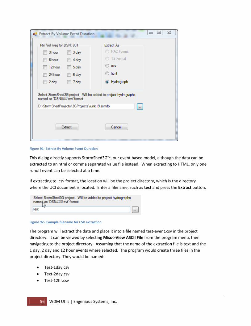
56 WDM Utils | Engenious Systems, Inc.
Figure 91- Extract By Volume Event Duration
This dialog directly supports StormShed3G™, our event based model, although the data can be
extracted to an html or comma separated value file instead. When extracting to HTML, only one
runoff event can be selected at a time.
If extracting to .csv format, the location will be the project directory, which is the directory
where the UCI document is located. Enter a filename, such as test and press the Extract button.
Figure 92- Example filename for CSV extraction
The program will extract the data and place it into a file named test-event.csv in the project
directory. It can be viewed by selecting Misc->View ASCII File from the program menu, then
navigating to the project directory. Assuming that the name of the extraction file is text and the
1 day, 2 day and 12 hour events where selected. The program would create three files in the
project directory. They would be named:
Test-1day.csv
Text-2day.csv
Test-12hr.csv

Engenious Systems, Inc. | WDM Utils 57
HTML Format
If the method of extraction is to an HTML file, it will simply be placed in the WDM View window.
When extracting to HTML format, only one event can be extracted at a time.
Figure 93 - Example Html Extraction of Peak Volumes
Hydrograph Format
If the choice for extraction is to a StormShed3G hydrograph, then the user will also need to
select the StormShed3G project (see Figure 91). Assuming that the 12hr and 7day events are
selected for extraction, the StormShed3G project would contain:
Figure 94- StormShed3G hydrographs from HSPFToolkit
The events will be named DSN801-12hr and DSN801-7day.

58 WDM Utils | Engenious Systems, Inc.
Figure 95- StormShed3G 7 Day hydrograph plot
In StormShed3G, the hydrographs are easily plotted.
RAC and TS Formats
If the data set is a precipitation data set, then the RAC and TS formats are available. The RAC
format it a proprietary StormShed™ Rainfall distribution format. The program wants to know a
location to place the RAC file. There are two possible choices, the StormShed3G project
directory, or the location of the specified in the StormShed3G Misc->Config->Application Links
menu selection, in the Location of Local RAC/IDF/TSS files field.
Figure 96- StormShed3G Application Links Location
The RAC file is a normalized rainfall distribution curve file and acts the same as any other rainfall
distribution, such as the Type 2 or Type 1A distributions. It is an ASCII file and can be viewed in
Notepad. If viewed, the first line would be:
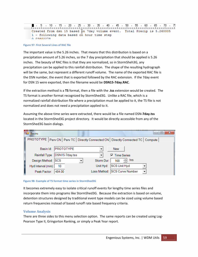
Engenious Systems, Inc. | WDM Utils 59
Figure 97- First Several Lines of RAC file
The important value is the 5.26 inches. That means that this distribution is based on a
precipitation amount of 5.26 inches, so the 7 day precipitation that should be applied is 5.26
inches. The beauty of RAC files is that they are normalized, so in StormSheh3G, any
precipitation can be applied to this rainfall distribution. The shape of the resulting hydrograph
will be the same, but represent a different runoff volume. The name of the exported RAC file is
the DSN number, the event that is exported followed by the RAC extension. If the 7day event
for DSN 15 were exported, then the filename would be DSN15-7day.RAC.
If the extraction method is a TS format, then a file with the .tss extension would be created. The
TS format is another format recognized by StormShed3G. Unlike a RAC file, which is a
normalized rainfall distribution file where a precipitation must be applied to it, the TS file is not
normalized and does not need a precipitation applied to it.
Assuming the above time series were extracted, there would be a file named DSN-7day.tss
located in the StormShed3G project directory. It would be directly accessible from any of the
StormShed3G basin dialogs.
Figure 98- Example of TS format time series in StormShed3G
It becomes extremely easy to isolate critical runoff events for lengthy time series files and
incorporate them into programs like StormShed3G. Because the extraction is based on volume,
detention structures designed by traditional event type models can be sized using volume based
return frequencies instead of based runoff rate based frequency criteria.
Volume Analysis
There are three sides to this menu selection option. The same reports can be created using Log-
Pearson Type II, Gringorton Ranking, or simply a Peak Year report.

60 WDM Utils | Engenious Systems, Inc.
Both the Log Pearson and Gringorton selections produce a massive report designed to compute
return frequencies (by volume) for a selected data set for events ranging from 3 hour to 7 days.
The report contains the volume of runoff from each year for each design event. At the bottom,
there is a table of return frequencies for each design event. So this generates a 2 year return
volume for a 3 hour event, 6 hour event, 12 hour event, etc.
Selection of the WDM Utils->Reports->Volume Analysis->Log Pearson Ranking menu selection:
Figure 99- Summary Return Freq by Log Pearson Type III
The same report can also be generated using the Gringorton Positioning method by selecting
WDM Utils->Reports->Volume Analysis->Plot Position Ranking menu selection instead.
Selection of Utils->Reports->Volume Analysis->Only Peak Year menu selection will return a
simple summary report listing the duration event, starting date and Maximum Volume.

Engenious Systems, Inc. | WDM Utils 61
Figure 100-Peak Volume Durations for DSN: 801
Time Series Plotting
Time Series Plotting is available by selecting the Utils->Reports->Volume Analysis->TS Plot
menu selection. The multiple datasets can be selected from the main WDM Utils.

62 WDM Utils | Engenious Systems, Inc.
Figure 101- TS Plot for DSN 701 and DSN 801
The plotting tool is very flexible. It can combine multiple time series. The page size can be
reconfigured to display from 1 day to 1 year on the graph. There is a slider on top that allows
the user to slide the display forward or backward in time. And the window frame that displays
the chart can be enlarged to the size of the computer monitor.
Saving the chart to a file is not supported (at this time). A Simple screen capture like the one
used to create this manual is perfect for reports.
Figure 102- Sample TS Plot selecting both Precipitation and Runoff Time Series
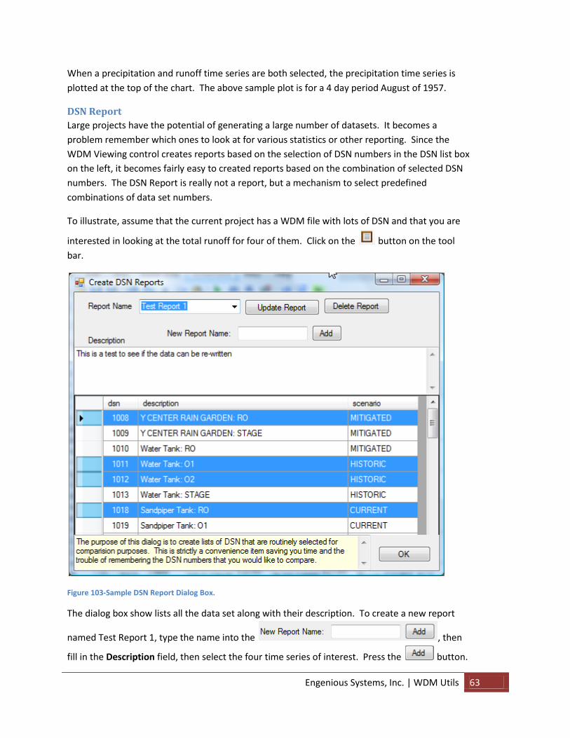
Engenious Systems, Inc. | WDM Utils 63
When a precipitation and runoff time series are both selected, the precipitation time series is
plotted at the top of the chart. The above sample plot is for a 4 day period August of 1957.
DSN Report
Large projects have the potential of generating a large number of datasets. It becomes a
problem remember which ones to look at for various statistics or other reporting. Since the
WDM Viewing control creates reports based on the selection of DSN numbers in the DSN list box
on the left, it becomes fairly easy to created reports based on the combination of selected DSN
numbers. The DSN Report is really not a report, but a mechanism to select predefined
combinations of data set numbers.
To illustrate, assume that the current project has a WDM file with lots of DSN and that you are
interested in looking at the total runoff for four of them. Click on the button on the tool
bar.
Figure 103-Sample DSN Report Dialog Box.
The dialog box show lists all the data set along with their description. To create a new report
named Test Report 1, type the name into the , then
fill in the Description field, then select the four time series of interest. Press the button.
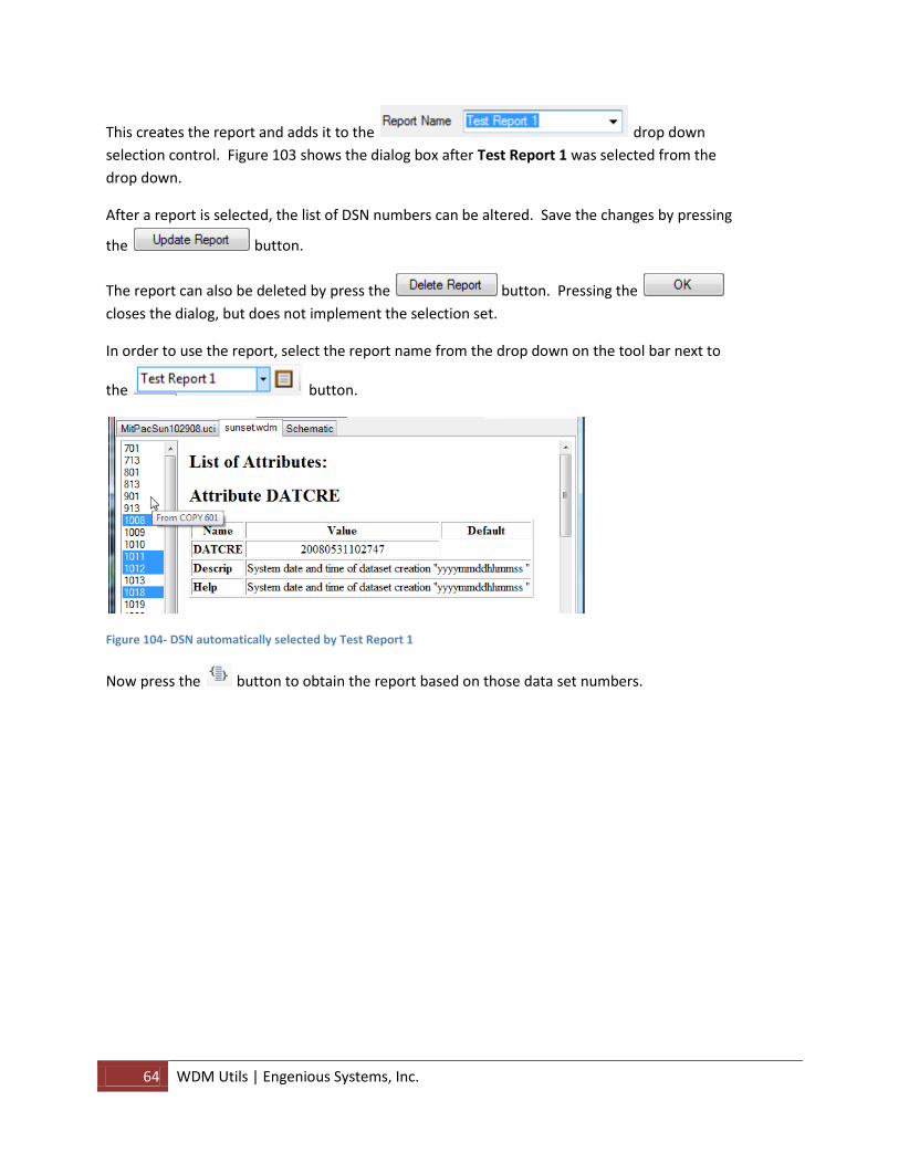
64 WDM Utils | Engenious Systems, Inc.
This creates the report and adds it to the drop down
selection control. Figure 103 shows the dialog box after Test Report 1 was selected from the
drop down.
After a report is selected, the list of DSN numbers can be altered. Save the changes by pressing
the button.
The report can also be deleted by press the button. Pressing the
closes the dialog, but does not implement the selection set.
In order to use the report, select the report name from the drop down on the tool bar next to
the button.
Figure 104- DSN automatically selected by Test Report 1
Now press the button to obtain the report based on those data set numbers.
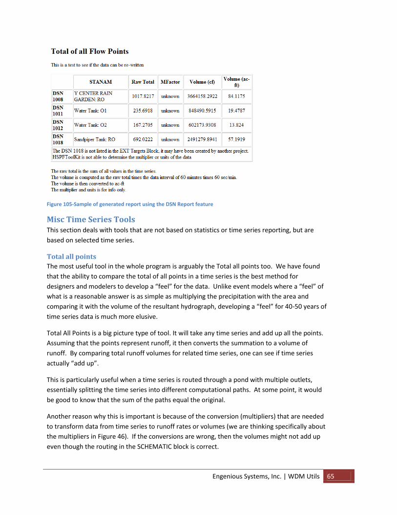
Engenious Systems, Inc. | WDM Utils 65
Figure 105-Sample of generated report using the DSN Report feature
Misc Time Series Tools This section deals with tools that are not based on statistics or time series reporting, but are
based on selected time series.
Total all points
The most useful tool in the whole program is arguably the Total all points too. We have found
that the ability to compare the total of all points in a time series is the best method for
designers and modelers to develop a “feel” for the data. Unlike event models where a “feel” of
what is a reasonable answer is as simple as multiplying the precipitation with the area and
comparing it with the volume of the resultant hydrograph, developing a “feel” for 40-50 years of
time series data is much more elusive.
Total All Points is a big picture type of tool. It will take any time series and add up all the points.
Assuming that the points represent runoff, it then converts the summation to a volume of
runoff. By comparing total runoff volumes for related time series, one can see if time series
actually “add up”.
This is particularly useful when a time series is routed through a pond with multiple outlets,
essentially splitting the time series into different computational paths. At some point, it would
be good to know that the sum of the paths equal the original.
Another reason why this is important is because of the conversion (multipliers) that are needed
to transform data from time series to runoff rates or volumes (we are thinking specifically about
the multipliers in Figure 46). If the conversions are wrong, then the volumes might not add up
even though the routing in the SCHEMATIC block is correct.
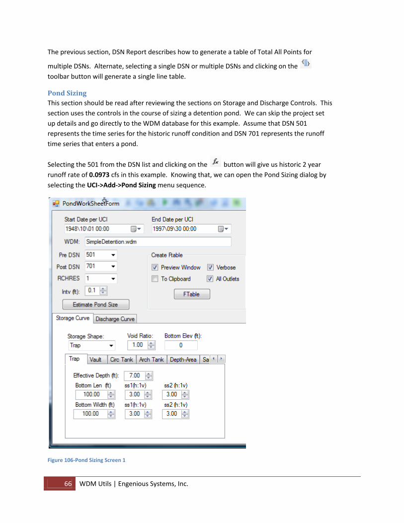
66 WDM Utils | Engenious Systems, Inc.
The previous section, DSN Report describes how to generate a table of Total All Points for
multiple DSNs. Alternate, selecting a single DSN or multiple DSNs and clicking on the
toolbar button will generate a single line table.
Pond Sizing
This section should be read after reviewing the sections on Storage and Discharge Controls. This
section uses the controls in the course of sizing a detention pond. We can skip the project set
up details and go directly to the WDM database for this example. Assume that DSN 501
represents the time series for the historic runoff condition and DSN 701 represents the runoff
time series that enters a pond.
Selecting the 501 from the DSN list and clicking on the button will give us historic 2 year
runoff rate of 0.0973 cfs in this example. Knowing that, we can open the Pond Sizing dialog by
selecting the UCI->Add->Pond Sizing menu sequence.
Figure 106-Pond Sizing Screen 1
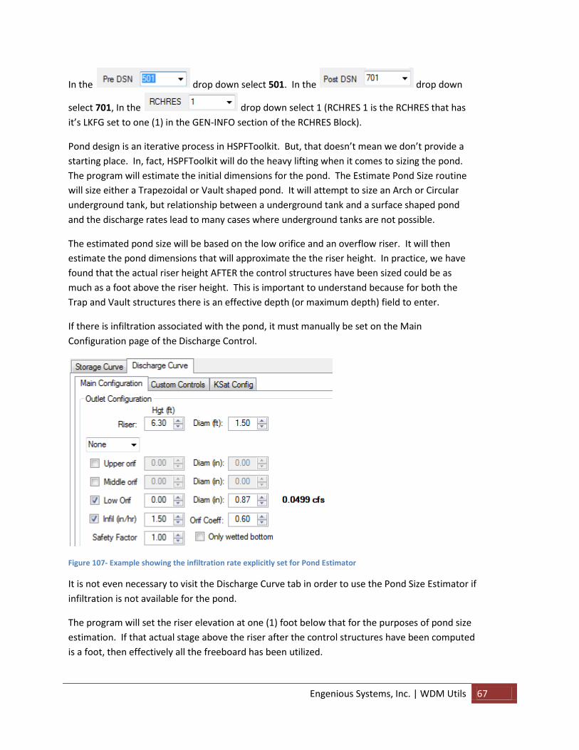
Engenious Systems, Inc. | WDM Utils 67
In the drop down select 501. In the drop down
select 701, In the drop down select 1 (RCHRES 1 is the RCHRES that has
it’s LKFG set to one (1) in the GEN-INFO section of the RCHRES Block).
Pond design is an iterative process in HSPFToolkit. But, that doesn’t mean we don’t provide a
starting place. In, fact, HSPFToolkit will do the heavy lifting when it comes to sizing the pond.
The program will estimate the initial dimensions for the pond. The Estimate Pond Size routine
will size either a Trapezoidal or Vault shaped pond. It will attempt to size an Arch or Circular
underground tank, but relationship between a underground tank and a surface shaped pond
and the discharge rates lead to many cases where underground tanks are not possible.
The estimated pond size will be based on the low orifice and an overflow riser. It will then
estimate the pond dimensions that will approximate the the riser height. In practice, we have
found that the actual riser height AFTER the control structures have been sized could be as
much as a foot above the riser height. This is important to understand because for both the
Trap and Vault structures there is an effective depth (or maximum depth) field to enter.
If there is infiltration associated with the pond, it must manually be set on the Main
Configuration page of the Discharge Control.
Figure 107- Example showing the infiltration rate explicitly set for Pond Estimator
It is not even necessary to visit the Discharge Curve tab in order to use the Pond Size Estimator if
infiltration is not available for the pond.
The program will set the riser elevation at one (1) foot below that for the purposes of pond size
estimation. If that actual stage above the riser after the control structures have been computed
is a foot, then effectively all the freeboard has been utilized.

68 WDM Utils | Engenious Systems, Inc.
Figure 108- Initial Trap Pond Settings
Assuming that the above Trap Pond settings are initially set as specified above. The most
important number, other than the side slopes is the Effective Depth of 10 ft. Pressing the
button will open the estimator.
Figure 109 - Pond Size Estimator
The estimator allows the user to modify the initial starting bottom width. More importantly, it
allows the user to override the pond depth. As we described in the preceding paragraph, the
program looks at the Effective depth, and assumes that the riser will be one (1) foot below it.
Here we can change the riser elevation by modifying the Pond Depth setting.

Engenious Systems, Inc. | WDM Utils 69
A Length to Width ratio can also be specified. In this example, we will change the Pond Depth to
and the Bottom Width to . Pressing the
button will start the computation. Selecting the will enable the
button. This is provided to stop the computation for whatever reason.
Actually, it is there to stop the computation in case the program fails to catch a stop point and
keeps running endlessly.
Figure 110 - Pond Estimator Results
The program will run and update the Score, Stage, Orif Diam, and Approx Pond Vol fields.
Actually, the Orifice Diameter is determined at the start of the computation, and the other fields
are updated with each iteration. When the computation has finished, the
button will be disabled again. The estimator will report the Orifice Diameter that was used in
the computations. It also reports the approximate pond stage. This is only an estimate of what
the final pond stage will be after the control structures are actually designed. The
check box will allow for the manual estimation of the pond size.
Sizing the pond is based on the Score. The whole idea is to attempt pond dimensions that will
give the lowest score above zero. THAT is NOT TO SAY that the closer one gets to zero the more
accurate the approximation! It isn’t related. It is just a score to indicate if it isn’t worth
attempting any further adjustments. The program stops when it has found a pond dimension
(Bottom Width) that is accurate to one (1) ft. In this current example the Bottom Width
accompanying the final answer is . At 104 ft, the score would have
returned a number less than zero.
Clicking on the button will transfer the dimensions back to the worksheet.

70 WDM Utils | Engenious Systems, Inc.
Figure 111-Discharge Structure Configuration
The Discharge Control shows the and
. This is a reflection of the Pond Estimator.
Check the check box and press the button.
Figure 112 - Results Plot 1

Engenious Systems, Inc. | WDM Utils 71
This is due to the fact that the Pond Estimator only estimated the pond size, the lowest orifice
with an overflow riser. To address the issue, specify another control structure and such as a vee
weir, , and modify the riser elevation to
and press the button to see the results.
Figure 113- Results Plot 2
The selection and size of each control structure is up to the user, and is essentially a trial and
error process. We find that it generally goes very quickly once the approximate pond size has
been determined. In this case, the final results were:
Figure 114- Final Routing Results
The mixture of the control structures resulted in a peak stage of 6.44 ft and a maximum pond
volume of about 100,270 cf. Figure 110 estimated that the final peak stage to be about 6.2 ft
and the volume to be somewhere between 95,500 and 116,500 cf.
To be honest, in this example we were lucky. Depending on the pond shape and mix of control
structures, we have found that the final stage could be as much as 30% higher!
More info about the Pond Worksheet
Looking at a close up of the plot, there might be an instance where there is a small section in
yellow.
Figure 115- Close up of the Plot

72 WDM Utils | Engenious Systems, Inc.
That is a visual cue that the segment is on the wrong side of the red line. Also if the
button is unchecked, a tabular display of the results is presented. There will be
a line or several :
Figure 116 - Chart view of Routing results.
Indicating that there some points did not pass the compliance criteria.
There are a lot of numeric up-down fields in the storage and discharge controls. These fields
have been customized of mouse only interaction. Placing the mouse cursor in the editing
portion of any of these fields and right-mouse clicking will present a pop-up menu with at least
two choices:
Figure 117-Change Increment and Decimal places
Selecting the Change Increment will present another pop-up that allows changing the up-down
arrows to alter the number at a different increment, perhaps changing the control from
incrementing at 0.1 ft increments to 0.01 ft increments.
Selecting the Decimal Places menu item changes the decimal places that are displayed, such as
from 2 decimal places to 4 decimal places. These are provided to free up the other hand to hold
a cup of coffee!
Below the compliance plot:
Figure 118-Compliance Plot information panel
This reports the peak stage in the pond as well as the maximum pond volume at the peak stage.
Iterations are extremely fast, 1-2 seconds for a 40 year event.
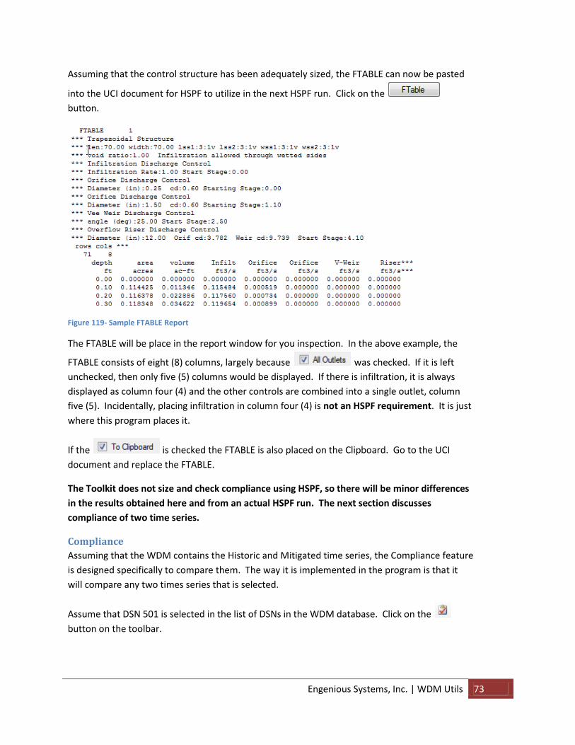
Engenious Systems, Inc. | WDM Utils 73
Assuming that the control structure has been adequately sized, the FTABLE can now be pasted
into the UCI document for HSPF to utilize in the next HSPF run. Click on the
button.
Figure 119- Sample FTABLE Report
The FTABLE will be place in the report window for you inspection. In the above example, the
FTABLE consists of eight (8) columns, largely because was checked. If it is left
unchecked, then only five (5) columns would be displayed. If there is infiltration, it is always
displayed as column four (4) and the other controls are combined into a single outlet, column
five (5). Incidentally, placing infiltration in column four (4) is not an HSPF requirement. It is just
where this program places it.
If the is checked the FTABLE is also placed on the Clipboard. Go to the UCI
document and replace the FTABLE.
The Toolkit does not size and check compliance using HSPF, so there will be minor differences
in the results obtained here and from an actual HSPF run. The next section discusses
compliance of two time series.
Compliance
Assuming that the WDM contains the Historic and Mitigated time series, the Compliance feature
is designed specifically to compare them. The way it is implemented in the program is that it
will compare any two times series that is selected.
Assume that DSN 501 is selected in the list of DSNs in the WDM database. Click on the
button on the toolbar.

74 WDM Utils | Engenious Systems, Inc.
Figure 120- Compliance Dialog
When this dialog opens, DSN 501 is already filled in and cannot be changed. This is because it
was selected in the WDM view list box. Select DSN 801 as the DSN to evaluate. The remainder
of the dialog allows the customization of the compliance criteria. The typical compliance
requirement is 50% of the 2-year return frequency (by rate) through the 50-year return
frequency. This program defaults to 25 steps but it is not uncommon to require a match up to
100 steps between the upper and lower threshold values.
The Straight Line Analysis is a straight line between the upper and lower threshold values,
whereas the Tailored Analysis is reduces the compliance requirement to the major return
frequencies. The program support compliance using either Log-Pearson or Plotting Position.
Clicking on the Analyze button presents the compliance chart:

Engenious Systems, Inc. | WDM Utils 75
Figure 121- Compliance Chart
In addition, the Compliance Table is generated for the WDM Report View.
Figure 122-WDM Report View show Compliance
Although the Compliance criteria can be changed or adjusted in the Compliance Dialog, it can be
“set” in the program Preferences.

76 WDM Utils | Engenious Systems, Inc.
Water Quality
The Computation of water quality flows for time series data sets is also available to the program.
Water Quality is interesting and we have a thorough discussion of it in our “HSPF For Dummies”
publication. In any case, as implemented by this program, there is the ability to compute water
quality flows for any time series.
First select a DSN in the WDM View list that water quality analysis should be performed.
Go to the section titled Basin Areas and compute the areas for the DSN that you want Water
Quality analysis. Click on the button on the toolbar.
Figure 123- Water Quality Calculator
The %Till and % Impervious is from the Basins Areas. The DSN 801 is the currently selected Data
set. Click on the button and a report will be generated for DSN 801.

Engenious Systems, Inc. | WDM Utils 77
Figure 124 - Water Quality Computation.
Although the Water Quality Runoff is defined as capturing 91% of the total simulated runoff
volume, this dialog allows the user to change the percentage that is captured.
New WDM
HSPF Toolkit has the ability to create new WDM databases populated with the DSNs that are
specified in the EXT TARGETS Block. There is a problem with creating new WDM databases. The
problem is that most WDM databases include EVAP and PREC time series, so creating a new
WDM file would not contain those time series.
In order to successfully use this feature the UCI document must use two (2) WDM files.
Figure 125-Example of UCI that specifies two WDM files
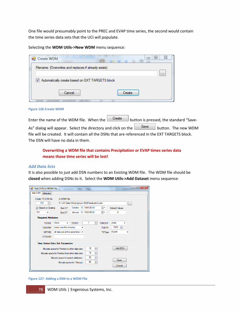
78 WDM Utils | Engenious Systems, Inc.
One file would presumably point to the PREC and EVAP time series, the second would contain
the time series data sets that the UCI will populate.
Selecting the WDM Utils->New WDM menu sequence:
Figure 126-Create WDM
Enter the name of the WDM file. When the button is pressed, the standard “Save-
As” dialog will appear. Select the directory and click on the button. The new WDM
file will be created. It will contain all the DSNs that are referenced in the EXT TARGETS block.
The DSN will have no data in them.
Overwriting a WDM file that contains Precipitation or EVAP times series data
means those time series will be lost!
Add Data Sets
It is also possible to just add DSN numbers to an Existing WDM file. The WDM file should be
closed when adding DSNs to it. Select the WDM Utils->Add Dataset menu sequence:
Figure 127- Adding a DSN to a WDM File

Engenious Systems, Inc. | WDM Utils 79
Select the WDM file to add the DSN.
Specify the new DSN number.
If it is to be based on a DSN that is already in the WDM select
checkbox and then select the DSN that is to be used as a template.
If the starting date is earlier than the year shown in the TSBYR selector
, it needs to be adjusted. Typically adjust it down to the next
decade.
If you anticipate x years worth of data, be certain that the year in
plus x years of data is more than the ending year of your data.
Generally, only the default attributes will be written to the WDM file, however, selection of
the Attributes tab will enable the addition of attributes and also allow the values of those
attributes to be set. When finished modifying the attribute list (if necessary), click on the
button. The DSN is saved to memory. It is OK to click on the button multiple
times, if the DSN already exists, it will respond with a message box.
When finished adding DSNs, click on the button to commit the additions and
update the WDM file.


Engenious Systems, Inc. | Schematic Layout 81
Schematic Layout Much of the focus on the implementation of a schematic layout view for the UCI document revolves
around the ability to create a layout view from an existing UCI document. This section discusses all the
features in the context of how it deals with an existing UCI.
The impact is that there is not a clear path to create a UCI from a schematic layout at this time. We are
working on it.
The schematic layout view depends on the definition of SUBBSN sub blocks in the SCHEMATIC Block
section of the UCI document. The SUBBSN sub block has been discussed (see Figure 42) and will not be
repeated here. Once SUBBSN blocks have been defined, just press the tab.
Figure 128- Auto Layout Create
This dialog gives users the opportunity to specify an offset on the x-axis and grid spacing between nodes
that will be inserted. If there are a lot of basins and reaches, a smaller grid spacing would probably be
better, if this is a small project, then the larger size would work fine. Press the Auto-Create button.
There will probably be several warning dialogs, not to worry.
For a one basin, one RCHRES UCI document will look like this.

82 Schematic Layout | Engenious Systems, Inc.
Figure 129- Layout Example 1
The grid leaves a whole lot to be desired, but it is a starting point. Fortunately, all objects in the
schematic can be repositioned, so to clean it up:
Figure 130- Layout 1 Cleaned up
The primary elements in the layout are the SUBBSNs, RCHRESs, COPY and POA nodes. The mouse is very
active in the layout view. Allowing it to hover over a node or connector and information about it will
appear in a tool tip.
SUBBSN nodes
Double clicking on a SUBBSN node will present the Basin Dialog. In this case we have double
clicked on SUBBSN 1.

Engenious Systems, Inc. | Schematic Layout 83
Figure 131 - Basin Dialog
Things that can be done from this dialog are:
Rename the sub-basin.
Add additional land uses to it.
Modify the area from each land use.
Assign MASS-LINK targets to it.
What can’t be done is assign target nodes to it. Assigning a target node is drawing the node that is
downstream of this one. Do that by drawing it. The Target Nodes represent the nodes that are
downstream of the sub basin. In this case, looking at Figure 130, there really is a COPY 1 and RCHRES 1
connected to this sub basin. Looking at this dialog, it is clear that there is a one PERLND (C,Lawn, Mod)
and it targets a COPY 1 and a RCHRES 1. MASS-LINK 12 specifies what is transferred from this sub basin
to COPY 1.
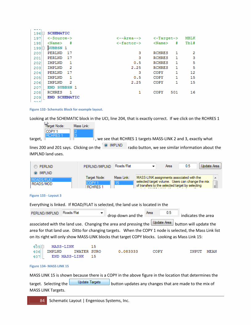
84 Schematic Layout | Engenious Systems, Inc.
Figure 132- Schematic Block for example layout.
Looking at the SCHEMATIC block in the UCI, line 204, that is exactly correct. If we click on the RCHRES 1
target, , we see that RCHRES 1 targets MASS-LINK 2 and 3, exactly what
lines 200 and 201 says. Clicking on the radio button, we see similar information about the
IMPLND land uses.
Figure 133 - Layout 3
Everything is linked. If ROAD/FLAT is selected, the land use is located in the
drop down and the indicates the area
associated with the land use. Changing the area and pressing the button will update the
area for that land use. Ditto for changing targets. When the COPY 1 node is selected, the Mass Link list
on its right will only show MASS-LINK blocks that target COPY blocks. Looking as Mass Link 15:
Figure 134- MASS LINK 15
MASS LINK 15 is shown because there is a COPY in the above figure in the location that determines the
target. Selecting the button updates any changes that are made to the mix of
MASS LINK Targets.
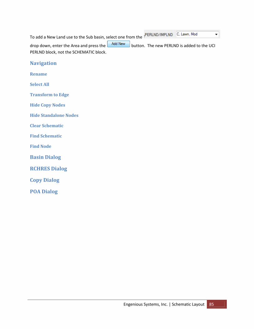
Engenious Systems, Inc. | Schematic Layout 85
To add a New Land use to the Sub basin, select one from the
drop down, enter the Area and press the button. The new PERLND is added to the UCI
PERLND block, not the SCHEMATIC block.
Navigation
Rename
Select All
Transform to Edge
Hide Copy Nodes
Hide Standalone Nodes
Clear Schematic
Find Schematic
Find Node
Basin Dialog
RCHRES Dialog
Copy Dialog
POA Dialog

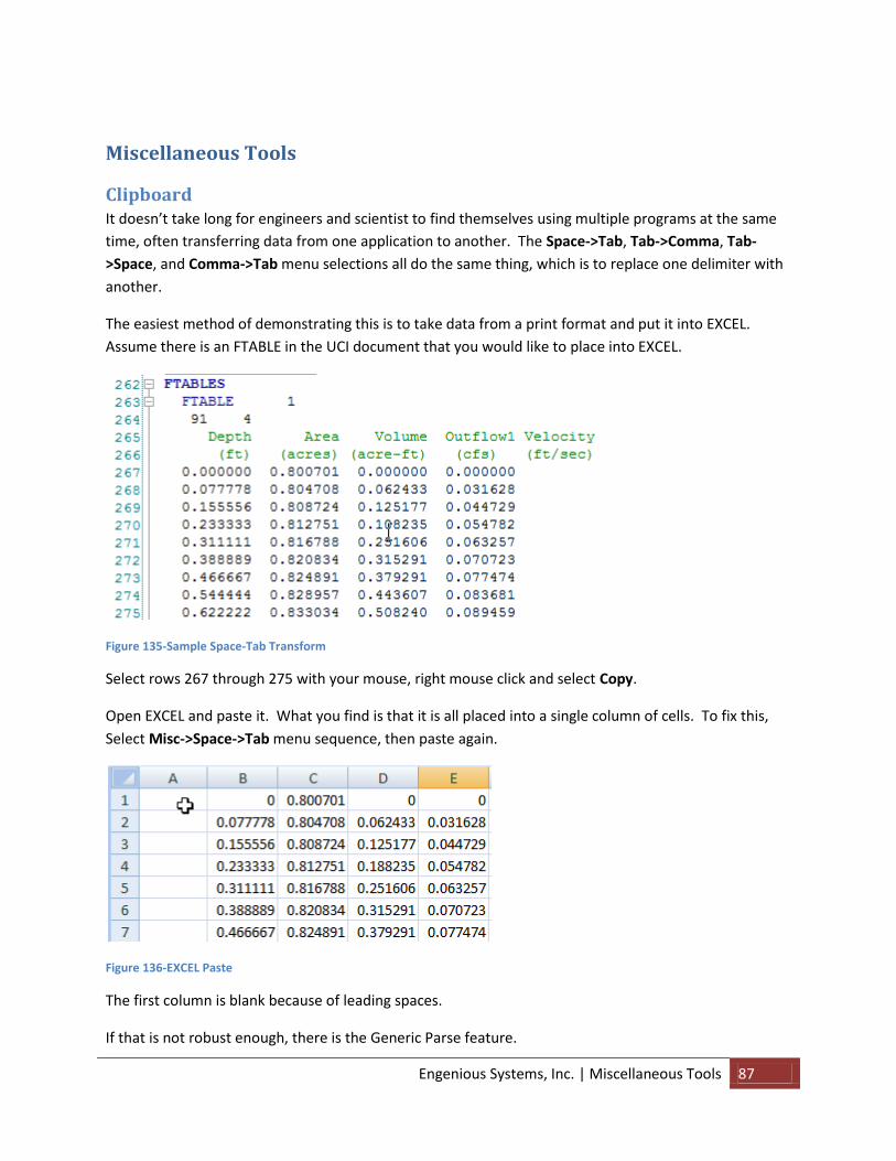
Engenious Systems, Inc. | Miscellaneous Tools 87
Miscellaneous Tools
Clipboard It doesn’t take long for engineers and scientist to find themselves using multiple programs at the same
time, often transferring data from one application to another. The Space->Tab, Tab->Comma, Tab-
>Space, and Comma->Tab menu selections all do the same thing, which is to replace one delimiter with
another.
The easiest method of demonstrating this is to take data from a print format and put it into EXCEL.
Assume there is an FTABLE in the UCI document that you would like to place into EXCEL.
Figure 135-Sample Space-Tab Transform
Select rows 267 through 275 with your mouse, right mouse click and select Copy.
Open EXCEL and paste it. What you find is that it is all placed into a single column of cells. To fix this,
Select Misc->Space->Tab menu sequence, then paste again.
Figure 136-EXCEL Paste
The first column is blank because of leading spaces.
If that is not robust enough, there is the Generic Parse feature.

88 Miscellaneous Tools | Engenious Systems, Inc.
Figure 137-Generic Parse.
Place your text on the clipboard, and specify the character to replace and the character to replace it
with. Then paste wherever it is needed.
Extract Column From Clipboard
Tab to FTABLE Going back to Figure 136, suppose you created an FTABLE in EXCEL and then wanted to place it in the
UCI document, it can’t be done with a simple cut and paste. It can be done with our Tab->FTABLE
command. Copy the FTABLE cells from EXCEL to the Windows Clipboard.
Navigate to the location in the UCI Document where it is to pasted. MAKE SURE the cursor is placed in
the first position on the line where it is to be pasted! Then select Misc->Tab->Ftable. This feature does
not update the row and column count, but all the columns are lined up properly!
Stage Lookup
Flow From Stage
View Ascii File
Preferences
External Programs
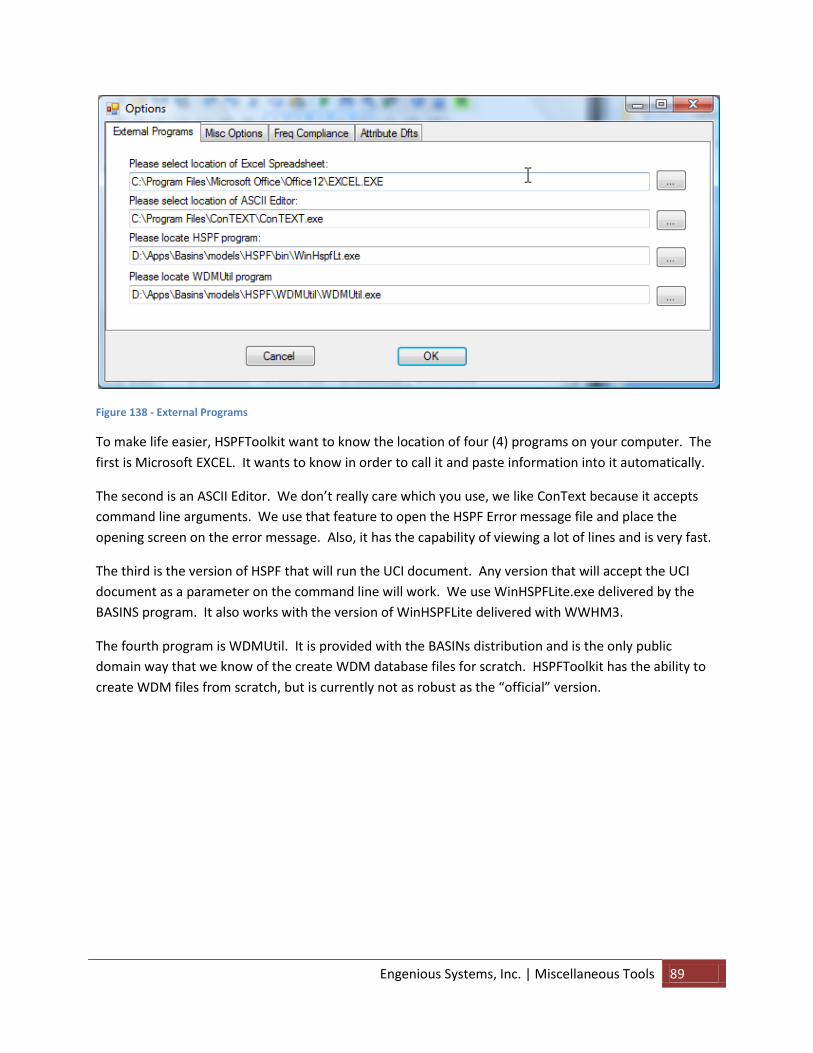
Engenious Systems, Inc. | Miscellaneous Tools 89
Figure 138 - External Programs
To make life easier, HSPFToolkit want to know the location of four (4) programs on your computer. The
first is Microsoft EXCEL. It wants to know in order to call it and paste information into it automatically.
The second is an ASCII Editor. We don’t really care which you use, we like ConText because it accepts
command line arguments. We use that feature to open the HSPF Error message file and place the
opening screen on the error message. Also, it has the capability of viewing a lot of lines and is very fast.
The third is the version of HSPF that will run the UCI document. Any version that will accept the UCI
document as a parameter on the command line will work. We use WinHSPFLite.exe delivered by the
BASINS program. It also works with the version of WinHSPFLite delivered with WWHM3.
The fourth program is WDMUtil. It is provided with the BASINs distribution and is the only public
domain way that we know of the create WDM database files for scratch. HSPFToolkit has the ability to
create WDM files from scratch, but is currently not as robust as the “official” version.

90 Miscellaneous Tools | Engenious Systems, Inc.
Misc Options
Figure 139- Misc Options, Preference Dialog
Automatically opening HSPF reports is off by default, primarily because we never look at them.
If you are working on a project and look at them after each run to figure out what has
happened, check this option.
Show all time series when opening WDM file. This is not checked by default. WDM files can
contain a lot of DSN numbers. Occasionally, there will be DSNs defined in the WDM that are not
used, so there is no point in showing them in the list of DSNs.
Display Return Frequency Charts. This is on be default because the charts look good when
demoing the program. Normally the tables are more important, so this defaults to on, but we
think most users will uncheck this until they need to write a report.
Show default values as blanks. This sets the default for the Generalized Editor.
Plotting Position Method. The default is Gringorton, however, we support Cunanne, Weibull,
Gumbel and also Log normal too. If you would rather use one of the others, this is the place to
tell the program.

Engenious Systems, Inc. | Miscellaneous Tools 91
Frequency Compliance
Figure 140- Preferences Frequency Compliance
This dialog sets the default for the Compliance Dialog. We set it up so that this controls the defaults of
the Compliance dialog and when using the Compliance dialog, you can over-ride the defaults.
Also, this is where the Skew and MSEG are set for non-Western Washington analysis. The defaults are
for Western Washington Only!!!!
Default Attributes
Figure 141- Preferences, Default Attributes

92 Miscellaneous Tools | Engenious Systems, Inc.
HSPFToolkit can create WDM files from scratch. All WDM files must have certain required Attributes.
We don’t need to explain Attributes at this time. This is the set of Attributes and the options that are
available to them. The toolkit can be like other applications that hardwire a certain type of WDM file.
We chose not to do that enabled this dialog so that users can create WDM files with different values in
the set of required Attributes.
Soils Logs

Engenious Systems, Inc. | Other 93
Other
HSPF Documentation HSPF Documentation is available by selecting the Help->HSPF Documentation menu sequence.
WDMUtil Documentation WDM Util Documentation is available by selecting the Help->WDMUtil Documentation menu sequence.
About
Registration
Server URL This is a pointer to the authentication website.
Revision Log The Revision log appears whenever a new version of HSPFToolkit is posted on-line. To view the log,
select this menu item.


Engenious Systems, Inc. | Other 95
Toolbar Symbols
New UCI
Open UCI
Save UCI
Save As UCI
Undo UCI
Redo UCI
Cut from UCI
Paste to UCI
Run HSPF
Find
Find Next
Replace
Reformat Line
Copy Down
Comment Toggle
Open WDM
DSN Summary
Log-Pearson Type III
(rate)
Peak Yearly Flows
Ranked Yearly Flows
Return Years (rate)
Plotting Position
Log Pearson Type III
(volume)
Peak Yearly Volume
Ranked Yearly
Volume
Return Years (vol)
Plotting Position (vol)
Total All Points
Compliance
Water Quality
HSPF Catalog
Conversions
DSN Report
Bookmark toggle
Next bookmark
Previous bookmark
Clear bookmarks
Collapse Outline
Expand Outline


Engenious Systems, Inc. | Other 97


Engenious Systems, Inc. | Equations 99
Equations
Vault A vault is the simplest of storage structures. It is generally treated as an open structure, meaning that
the stage will rise to whatever is necessary to complete the computation. It is up to the engineer to
decide if there is enough physical space to accommodate the storage depth.
lwdv
Where:
l= length in ft or m
w= width in ft or m
d= depth in ft or m
v= volume in cf or cm.
Trapezoidal The Trapezoidal shaped detention pond is the most common open detention pond. The pond features a
bottom area and side slopes on four sides. Typically the side slopes can vary.
3/dhdisthdistdwlv wlmm
Where:
2
21 ssl
llhdist
2
21 ssw
wwhdist
lm dhdistl Average length (ft or m)
wm dhdistw Average width (ft or m)
sxl = side slope on length side xh:1v
sxw = side slope on width side, xh:1v
Underground Pipe The volume of pipes used for detention storage is simply the area times the length of the pipe. To
support pipes on a slope, we break up the pipe into various components and use average end areas to
come up with a rating curve. The following sketch shows the various sections.

100 Equations | Engenious Systems, Inc.
BDBL
B
DYH
BL
Ys
costan0
cos0
tan0
Where
VolA = Volume of pipe fully occupied by water
VolB= Volume of pipe partially occupied by water
H= Water depth measured from the I.E. of the inlet end of the pipe
HA= Wetted water depth at the downstream end.
HB= Wetted water depth at the upstream end.
Circular
The volume of a circular pipe is simply the area of the circle multiplied by the length.
Arch
The volume of an arch section is simply the area of the arch multiplied by the length. The area of the
arch is computed based on Tables of Hydraulic Ratio published in Modern Sewer Design, Third Edition,
American Steel Institute, 1995.
Ellipse
The volume of an ellipse section is simply the area of the ellipse multiplied by the length. The area of the
ellipse is based on equations given in Engineering Mathematics Handbook, Second Edition, McGraw-Hill
Book Company, Jan J. Tuma, PhD
Stage-Storage They are described as stage-Area -Volume. On flats surfaces it is not a problem, on sloped surfaces, such
as a reach, volume is based on cross-sectional areas at upper and lower ends. The Area is the top
surface area.

Engenious Systems, Inc. | Equations 101
Rectangular Weir These weirs have large capacity, but have less sensitivity for flow measurement. The rectangular weir is
also known as a notch weir. The program offers two choices for weir flow computation. The standard
choice is an equation based on varying Coefficients with head. The weir coefficient is based on ratio
between the head on the weir crest and the height above the bottom of the pond.
Figure 142: Rectangular Weir
Practical design limits for the rectangular weir are:
H >= 0.03 meters;
H/p1 <= 2 and p1 >= 0.1 meters;
L >= 0.15 meters
The tail water level should be at least 0.05 meters below the weir crest.
Where:
H is the depth of flow above the weir.
p1 is the height from the weir crest to the bottom of the approach channel;
L is the length of the weir.
Discharges are computed based on the following equation:

102 Equations | Engenious Systems, Inc.
Q cLH 1 5.
Where Q is the discharge rate in cfs; L is the crest length (ft); H is the stage above the crest (ft); and c is
given by the equation:
cH
p 327 0 4. .
Where p is the height of the weir above the bottom.
The second method is a constant coefficient of 3.33.
In both cases a transition head is computed as:
Ht=1.60(1.0-B/L) + 1.08
Where :
Ht is the depth above the orifice bottom where discharges changes from weir to orifice flow.
B is the effective weir length
L is the weir length.
Orifice flow is based on a coefficient of 0.61 applied to the centroid of the opening.
Vee These weirs have greater control under low flow conditions. This weir is either a sharp or broad crested
vee shaped weir. The angle of the vee can vary from greater than zero degrees to 180 degrees. It
cannot be zero or 180 degrees.
The following are design limits for practical applications of sharp crested V-Notch weirs:
H/p1 <= 1.2
H/B <= 0.4 and B >= 0.6m;
0.60 >= H >= 0.05 m;
p1 >= 0.10 m;
100 deg >= theta >= 25 deg;
tailwater level >= 0.05 m below the vertex of the V-Notch.
V-Notch sharp crested weir coefficients
Notch angle (degrees) 20 40 60 80 100
Ce 0.595 0.581 0.577 0.577 0.580

Engenious Systems, Inc. | Equations 103
Kh(mm) 2.8 1.8 1.2 0.85 0.80
Figure 143: Triangular or Vee Weir
Kindsvater and Carter (1957) proposed that the discharge coefficient is a function of the notch
angle and effective head (he) on the weir. The effective head is the head on the weir corrected
by a correction factor kh such that he = h1 + Kh
This program uses the simplified formula:
5.2
2tan HcQ
Where
c is the orifice coefficient;
theta is the weir angle and
H is the stage above the crest elevation (ft).
Values of c are computed at runtime based on the following graph:
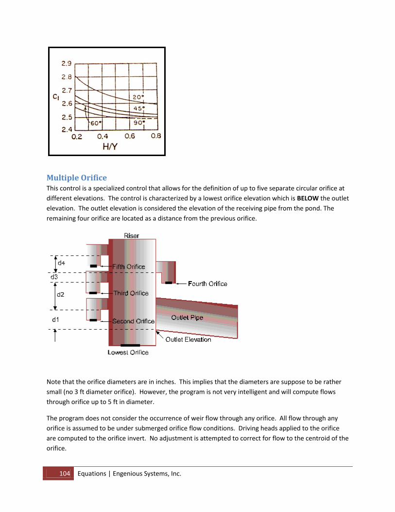
104 Equations | Engenious Systems, Inc.
Multiple Orifice This control is a specialized control that allows for the definition of up to five separate circular orifice at
different elevations. The control is characterized by a lowest orifice elevation which is BELOW the outlet
elevation. The outlet elevation is considered the elevation of the receiving pipe from the pond. The
remaining four orifice are located as a distance from the previous orifice.
Note that the orifice diameters are in inches. This implies that the diameters are suppose to be rather
small (no 3 ft diameter orifice). However, the program is not very intelligent and will compute flows
through orifice up to 5 ft in diameter.
The program does not consider the occurrence of weir flow through any orifice. All flow through any
orifice is assumed to be under submerged orifice flow conditions. Driving heads applied to the orifice
are computed to the orifice invert. No adjustment is attempted to correct for flow to the centroid of the
orifice.

Engenious Systems, Inc. | Equations 105
The lowest orifice is simply a placeholder to identify where it physically is located. For hydraulic
computations, the elevation that matters is the outlet elevation. Flows through each orifice is
computed relative to the outlet elevation.
Vertical This is a standard orifice defined by area. The orifice can be sharp or rounded, circular, rectangular or
any other configuration. It is up to the user to specify the coefficient to apply to the orifice. No
provision is made to compute weir flows for the weir at low head conditions. It is assumed that the
orifice opening is submerged and that the orifice equation applies. This is typically not a problem for
small orifice, there would be a problem for large openings.
For circular sharp edged orifice, the following practical design limits are recommended:
edge distance >= d/2;
upstream channel cross-sectional area >= 10 times orifice area;
upstream submergence of top of orifice >= d;
h >= 0.03 m.
Where
h is the difference between upstream and downstream water surface elevations.
d is the orifice diameter.
Under fully contracted, submerged conditions, the discharge coefficient cd may be taken as 0.61 for
rectangular sharp crested orifice shapes.
Uses the orifice formula:
Q cA h 64 4.
where
c is the orifice coefficient;
A is the area of the opening in sf and
h is the driving head acting on the orifice.

106 Equations | Engenious Systems, Inc.
Typically 0.61 for a sharp crested orifice. Can be anything that is reasonable. Some typically
coefficients for sharp crested weirs:
Orifice Diameter (m) Cd - Free flow Cd - Submerged Flow
0.02 0.61 0.57
0.025 0.62 0.58
0.035 0.64 0.61
0.045 0.63 0.61
0.05 0.62 0.61
0.065 0.61 0.60
0.075 0.60 0.60
When the orifice is partially submerged, the program computes flow based on critical depth at the face
of the orifice.
𝑄 = 𝐴𝑐 𝑔𝐷𝑐
∝
𝑄 = 𝐴𝑐/𝑇
𝐻𝑖 = 𝑌𝑐 +𝐷𝑐
2
Where:
Q is the discharge at a given pond water surface elevation,
Yc is critical depth at the face of the circular orifice,
Ac is the cross-sectional area of flow at critical depth,
T is the top width of flow at the orifice opening for critical depth,
Dc is the hydraulic depth,
Hi is the head on the orifice, as measured from the water surface elevation of the
pond to the invert elevation of the orifice,
g is the acceleration due to gravity, and
α is a type of discharge coefficient (1.00)
Overflow Riser The overflow riser is simple a comparison between weir and orifice flow.
Orifice Eqn:
𝑄 = 𝐶𝐷2 ℎ
Where
Q is the orifice flow
C is the orifice coefficient, 3.782

Engenious Systems, Inc. | Equations 107
D is the diameter in ft
h is the head on the orifice.
The coefficient of 3.782 is equivalent to a standard orifice coefficient of 0.4713 times sqrt(64.4).
Weir Equation:
𝐶𝐷ℎ1.5
Where
C is the weir coefficient, 9.739
D is the D in ft
h is the head on the weir.
The coefficient of 9.739 is equivalent to a standard weir coefficient of 3.1 times PI.
The equations were taken from the SCS Riser Inflow Curves Chart, July 1975


Engenious Systems, Inc. | Equations 109


Engenious Systems, Inc. | HSPFToolKit for Reviewers 111
HSPFToolKit for Reviewers
Basin Areas Report
Regional Parameter Comparison
FTable Comparison Making sure that target stages match the results from the FTABLE
DSN Totals Comparison
Water Quality Target


Engenious Systems, Inc. | HSPFToolKit for Reviewers 113


Engenious Systems, Inc. | References 115
References
Stormwater Management Manual for Western Washington, Washington State Department of Ecology,
Water Quality Program, Feb 2005.
Guidelines for Determining Flood Flow Frequency (revised), Bulletin #17B, Interagency Advisory
Committee on Water Data, March 1982
HSPF Version 12 User’s Manual, National Exposure Research Laboratory, Office of Research and
Development, U.S. Environmental Protection Agency, Athens, Georgia.
Modern Sewer Design, American Iron and Steel Institute, Third Edition 1995.
Engineering Mathematics Handbook, Second Edition, Jan J. Tuma, PhD, McGraw-Hill Book Company,
1978.
Design Hydrology and Sedimentology for Small Catchments, C.T. Haan, B.J. Barfield, J.C. Hayes,
Academic Press, 1981.
Fundamentals of Hydraulic Engineering Systems, H.C. Hwang, Prentice-Hall Series in Environmental
Sciences, 1981.
Water and Wastewater Engineering Hydraulics, T.J. Casey, Oxford Science Publications, 1992.
Draft Programmers Manual for the Watershed Data Management (WDM) System, U.S. Geological
Survey, Water-Resources Investigations Report 91-xxxx, 1991


![Ultra-Wideband Log Periodic Dipole Antenna (LPDA) for ......Figure 1. Layout of the proposed log periodic dipole antenna (US-LPDA). U-shaped dipole elements or stubs -[15][10]. The](https://img.pdfslide.us/doc/110x75/60acd6df90f4f8088f078346/ultra-wideband-log-periodic-dipole-antenna-lpda-for-figure-1-layout-of.jpg)


![The “m” Exponent in Carbonate Petrophysics - GeoNeuraleThe “m” Exponent in Carbonate Petrophysics ... log(Rw/Ro) /Log(Phi)]: Figure ... vicinity of the transition zone, across](https://img.pdfslide.us/doc/110x75/5aa33a407f8b9a1f6d8e4e60/the-m-exponent-in-carbonate-petrophysics-geoneuralethe-m-exponent.jpg)