HOW TO WRITE THESES

WITH TWO LINE TITLES

BY

OZLEM KALINLI

Submitted in partial fulfillment of therequirements for the degree of

Master of Science in Electrical Engineeringin the Graduate College of theIllinois Institute of Technology

ApprovedAdvisor

Chicago, IllinoisMay 2003

c© Copyright by

OZLEM KALINLI

May 2003

ii

ACKNOWLEDGMENT

This dissertation could not have been written without Dr. X who not only

served as my supervisor but also encouraged and challenged me throughout my aca-

demic program. He and the other faculty members, Dr. Y and Dr. Z, guided me

through the dissertation process, never accepting less than my best efforts. I thank

them all.

(Don’t copy this sample text. Write your own acknowledgement.)

iii

TABLE OF CONTENTS

Page

ACKNOWLEDGEMENT . . . . . . . . . . . . . . . . . . . . . . . . . iii

LIST OF TABLES . . . . . . . . . . . . . . . . . . . . . . . . . . . . vi

LIST OF FIGURES . . . . . . . . . . . . . . . . . . . . . . . . . . . . vii

LIST OF SYMBOLS . . . . . . . . . . . . . . . . . . . . . . . . . . . viii

ABSTRACT . . . . . . . . . . . . . . . . . . . . . . . . . . . . . . . ix

CHAPTER

1. INTRODUCTION . . . . . . . . . . . . . . . . . . . . . . . 1

1.1. Basic Models . . . . . . . . . . . . . . . . . . . . . . . 11.2. Functional Series Methods in Linear Systems using Impulse

Response Generalization Algorithm . . . . . . . . . . . . 1

2. REPRESENTATION OF LINEAR CONSTRAINTS METHODSWITH CONVEX FUNCTION CONDITIONS IN MODERN OP-TIMIZATION THEORY . . . . . . . . . . . . . . . . . . . 5

2.1. Basic Concepts . . . . . . . . . . . . . . . . . . . . . . 52.2. Null and Range Spaces . . . . . . . . . . . . . . . . . . 52.3. Generating Null Space Matrices using VR Method . . . . . 52.4. Orthogonal Projection Matrix . . . . . . . . . . . . . . . 5

3. DUALITY AND SENSIVITY . . . . . . . . . . . . . . . . . 6

3.1. The Dual Problem . . . . . . . . . . . . . . . . . . . . 63.2. Duality Theory . . . . . . . . . . . . . . . . . . . . . . 6

4. NETWORK PROBLEMS . . . . . . . . . . . . . . . . . . . 7

4.1. Basic Examples . . . . . . . . . . . . . . . . . . . . . . 74.2. Basis Representation . . . . . . . . . . . . . . . . . . . 7

5. CONCLUSION . . . . . . . . . . . . . . . . . . . . . . . . 8

5.1. Summary . . . . . . . . . . . . . . . . . . . . . . . . . 8

APPENDIX . . . . . . . . . . . . . . . . . . . . . . . . . . . . . . . 9

A. TABLE OF TRANSITION COEFFICIENTS FOR THE DESIGNOF LINEAR-PHASE FIR FILTERS . . . . . . . . . . . . . . 9

iv

APPENDIX Page

B. NAME OF YOUR SECOND APPENDIX . . . . . . . . . . . 11

C. NAME OF YOUR THIRD APPENDIX . . . . . . . . . . . . 13

BIBLIOGRAPHY . . . . . . . . . . . . . . . . . . . . . . . . . . . . . 14

v

LIST OF TABLES

Table Page

1.1 Nonlinear Model Results . . . . . . . . . . . . . . . . . . . . . 2

1.2 Performance Analysis using Hard Decision Detection Method in Low-Level Noise Systems with Nonlinear Behavior . . . . . . . . . . . 3

vi

LIST OF FIGURES

Figure Page

1.1 An LNL Block Oriented Model Structure . . . . . . . . . . . . 3

1.2 Fuel Metabolism results with Method A . . . . . . . . . . . . . 4

1.3 Fuel Metabolism results using Method XYZ in complex systems forboth linear and Nonlinear behavior cases . . . . . . . . . . . . . 4

vii

LIST OF SYMBOLS

Symbol Definition

β probability of non-detecting bad data

δ Transition Coefficient Constant for the Design of Linear-Phase FIR Filters

ζ Reflection Coefficient Parameter

viii

ABSTRACT

Your Abstract goes here!

ix

1

CHAPTER 1

INTRODUCTION

1.1 Basic Models

In this chapter, we discuss the system identification problem for discrete-time

nonlinear dynamic systems. The discussion includes an overview of the representa-

tions of various nonlinear systems and their identification methods. Even though

some of these methods are developed for continuous-time system representations, we

only consider to work on the discrete-time representation of the nonlinear systems.

These techniques will guide us to develop the FPET model structure. The main

system equation we use here is:

x2 + y2 = z2 (1.1)

However, we will also represent a brief discuss on some more complex cases as well.

1.2 Functional Series Methods in Linear Systems using Impulse ResponseGeneralization Algorithm

One can represent a linear system by its impulse response. Volterra developed

a generalization of this representation for nonlinear systems in which the single im-

pulse response is replaced with a series of integration kernels. This generalization of

the impulse response, usually called Volterra series, can be used to approximate a

wide variety of systems. For instance, Boyd and Chua in [3]1 showed that a finite

Volterra series can be used to approximate any nonlinear operator which has fading

memory. This is explained in Section 1.1. Now you will see a listing example:

1. Suppression of hepatic glucose production

2. Stimulation of hepatic glucose uptake

1Corresponding to references in the Bibliography.

2

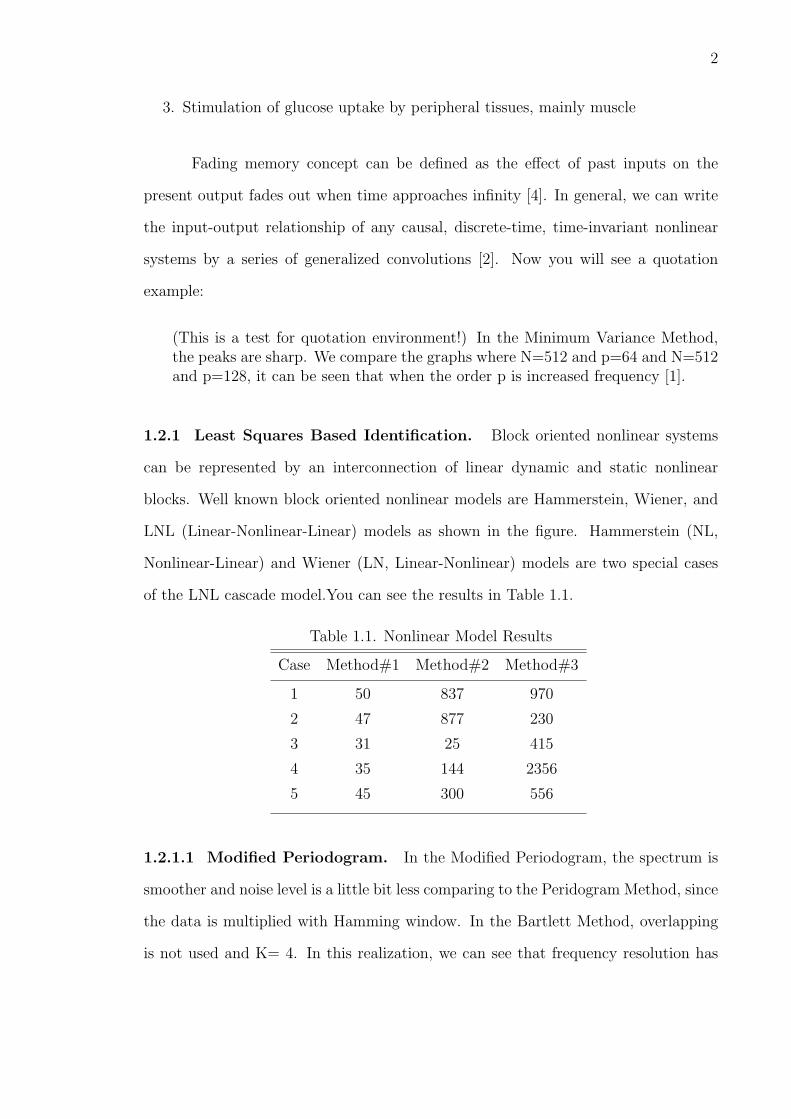
3. Stimulation of glucose uptake by peripheral tissues, mainly muscle

Fading memory concept can be defined as the effect of past inputs on the

present output fades out when time approaches infinity [4]. In general, we can write

the input-output relationship of any causal, discrete-time, time-invariant nonlinear

systems by a series of generalized convolutions [2]. Now you will see a quotation

example:

(This is a test for quotation environment!) In the Minimum Variance Method,the peaks are sharp. We compare the graphs where N=512 and p=64 and N=512and p=128, it can be seen that when the order p is increased frequency [1].

1.2.1 Least Squares Based Identification. Block oriented nonlinear systems

can be represented by an interconnection of linear dynamic and static nonlinear

blocks. Well known block oriented nonlinear models are Hammerstein, Wiener, and

LNL (Linear-Nonlinear-Linear) models as shown in the figure. Hammerstein (NL,

Nonlinear-Linear) and Wiener (LN, Linear-Nonlinear) models are two special cases

of the LNL cascade model.You can see the results in Table 1.1.

Table 1.1. Nonlinear Model Results

Case Method#1 Method#2 Method#3

1 50 837 970

2 47 877 230

3 31 25 415

4 35 144 2356

5 45 300 556

1.2.1.1 Modified Periodogram. In the Modified Periodogram, the spectrum is

smoother and noise level is a little bit less comparing to the Peridogram Method, since

the data is multiplied with Hamming window. In the Bartlett Method, overlapping

is not used and K= 4. In this realization, we can see that frequency resolution has

3

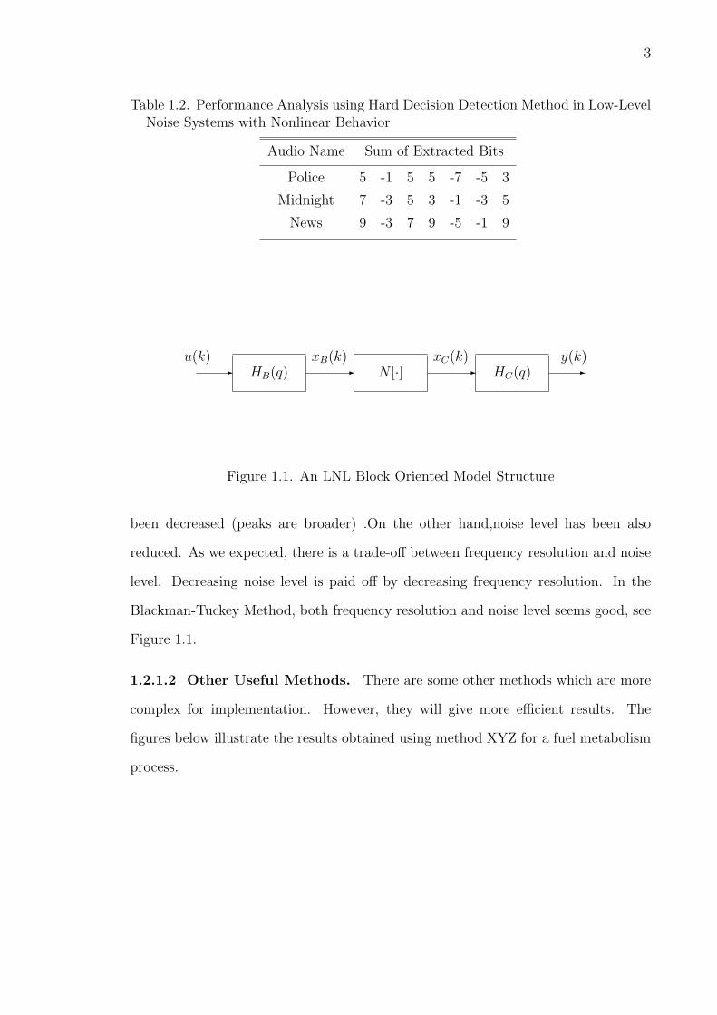
Table 1.2. Performance Analysis using Hard Decision Detection Method in Low-LevelNoise Systems with Nonlinear Behavior

Audio Name Sum of Extracted Bits

Police 5 -1 5 5 -7 -5 3

Midnight 7 -3 5 3 -1 -3 5

News 9 -3 7 9 -5 -1 9

HB(q) N [·] HC(q)- - - -u(k) y(k)xB(k) xC(k)

Figure 1.1. An LNL Block Oriented Model Structure

been decreased (peaks are broader) .On the other hand,noise level has been also

reduced. As we expected, there is a trade-off between frequency resolution and noise

level. Decreasing noise level is paid off by decreasing frequency resolution. In the

Blackman-Tuckey Method, both frequency resolution and noise level seems good, see

Figure 1.1.

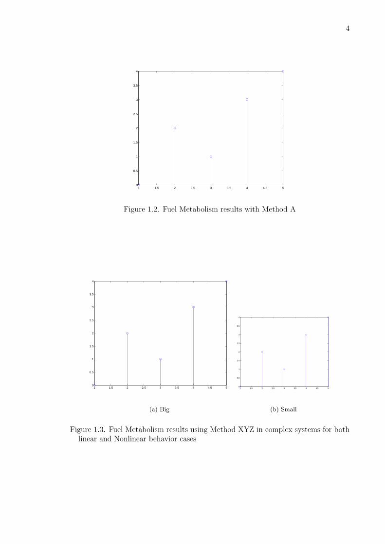
1.2.1.2 Other Useful Methods. There are some other methods which are more

complex for implementation. However, they will give more efficient results. The

figures below illustrate the results obtained using method XYZ for a fuel metabolism

process.

4

1 1.5 2 2.5 3 3.5 4 4.5 50

0.5

1

1.5

2

2.5

3

3.5

4

Figure 1.2. Fuel Metabolism results with Method A

1 1.5 2 2.5 3 3.5 4 4.5 50

0.5

1

1.5

2

2.5

3

3.5

4

(a) Big

1 1.5 2 2.5 3 3.5 4 4.5 50

0.5

1

1.5

2

2.5

3

3.5

4

(b) Small

Figure 1.3. Fuel Metabolism results using Method XYZ in complex systems for bothlinear and Nonlinear behavior cases

5

CHAPTER 2

REPRESENTATION OF LINEAR CONSTRAINTS METHODS WITH CONVEXFUNCTION CONDITIONS IN MODERN OPTIMIZATION THEORY

2.1 Basic Concepts

In this chapter we examine ways of representing linear constraints. The goal is

to write the constraints in a form that makes it easy to move from one feasible point

to another. The constraints specify interrelationship among the variables so that, for

example, if we increase the first variable, retaining feasibility might require making

a complicated sequence of changes to all the other variables. It is much easier if we

express the constraints using a coordinate system that is ”natural” for the constraints.

2 Then the interrelationship among the variables are taken care of by the coordinate

system, and moves between feasible points.

2.2 Null and Range Spaces

The null sapce of a matrix is orthogonal to the rows of that matrix......

2.3 Generating Null Space Matrices using VR Method

VR stands for Variable Reduction method. This is a simple method used in

linear programming ......

2.4 Orthogonal Projection Matrix

A matrix is called orthogonal projection if we have .......

2Natural means that the points be global optimums

6

CHAPTER 3

DUALITY AND SENSIVITY

3.1 The Dual Problem

For every linear programming problem there is a companion problem, called

dual linear problem...........

3.2 Duality Theory

There are two major results relating the primal and dual problems. The first

is called weak duality and is easier to prove.

7

CHAPTER 4

NETWORK PROBLEMS

4.1 Basic Examples

The most general network problem that we face with is called the minimum

cost network flow problem.

4.2 Basis Representation Many of the efficiencies in the network simplex method

come about because of the special form of the basis in the network problem.

8

CHAPTER 5

CONCLUSION

You need a Conclusion.tex file

5.1 Summary

This was just to create a sample section...

9

APPENDIX A

TABLE OF TRANSITION COEFFICIENTS FOR THE DESIGN OF

LINEAR-PHASE FIR FILTERS

10

Your Appendix will go here !

11

APPENDIX B

NAME OF YOUR SECOND APPENDIX

12

Your second appendix text....

13

APPENDIX C

NAME OF YOUR THIRD APPENDIX

14

Your third appendix text....

15

BIBLIOGRAPHY

[1] L. Boney, A. H. Tewfik, and K. N. Hamdy. Digital watermarks for audio signals.In Proceedings of the Third IEEE International Conference on Multimedia, pages473–480, June 1996.

[2] M. Goossens, F. Mittelbach, and A. Samarin. A LaTeX Companion. Addison-Wesley, Reading, MA, 1994.

[3] H. Kopka and P. W. Daly. A Guide to LaTeX. Addison-Wesley, Reading, MA,1999.

[4] D. Pan. A tutorial on mpeg/audio compression. IEEE Multimedia, 2:60–74,Summer 1995.