Clemson UniversityTigerPrints

All Theses Theses

5-2010

Compressive SensingYue MaoClemson University, yuem@clemson.edu

Follow this and additional works at: https://tigerprints.clemson.edu/all_theses

Part of the Applied Mathematics Commons

This Thesis is brought to you for free and open access by the Theses at TigerPrints. It has been accepted for inclusion in All Theses by an authorizedadministrator of TigerPrints. For more information, please contact kokeefe@clemson.edu.

Recommended CitationMao, Yue, "Compressive Sensing" (2010). All Theses. 853.https://tigerprints.clemson.edu/all_theses/853

Compressive Sensing

A Dissertation

Presented to

the Graduate School of

Clemson University

In Partial Fulfillment

of the Requirements for the Degree

Master of Sciences

Mathematical Sciences

by

Yue Mao

May 2010

Accepted by:

Dr. Shuhong Gao, Committee Chair

Dr. Taufiquar R Khan

Dr. Xiaoqian Sun

Abstract

Compressive sensing is a novel paradigm for acquiring signals and has a wide range of

applications. The basic assumption is that one can recover a sparse or compressible signal from

far fewer measurements than traditional methods. The difficulty lies in the construction of efficient

recovery algorithms. In this thesis, we review two main approaches for solving the sparse recovery

problem in compressive sensing: l1-minimization methods and greedy methods. Our contribution

is that we look at compressive sensing from a different point of view by connecting it with sparse

interpolation. We introduce a new algorithm for compressive sensing called generalized eigenvalues

(GE). GE uses the first m consecutive rows of discrete Fourier matrix as its measurement matrix.

GE solves for the support of a sparse signal directly by considering generalized eigenvalues of Hankel

systems. Under Fourier measurements, we compare GE with iterated hard thresholding (IHT) that

is one of the state-of-the-art greedy algorithms. Our experiment shows that GE has a much higher

probability of success than IHT when the number of measurements is small while GE is a bit more

sensitive for signals with clustered entries. To address this problem, we give some observations

from the experiment that suggests GE can be potentially improved by taking adaptive Fourier

measurements. In addition, most greedy algorithms assume that the sparsity k is known. As

sparsity depends on the signal and we may not be able to know the sparsity unless we have some

prior information about the signal. However, GE doesn’t need any prior information on the sparsity

and can determine the sparsity by simply computing the rank of the Hankel system.

Key words: compressive sensing, sparse recovery, generalized eigenvalues, sparse interpola-

tion, Hankel system, Fourier measurements

ii

Dedication

I dedicate this dissertation to all my loved ones, those with me today and those who have

passed on.

iii

Acknowledgments

I thank my advisor Shuhong Gao. His guidance, support, patience, and humor have made

this thesis possible. I also thank Frank Volny IV for his helpful discussion throughout the develop-

ment of this thesis and his comments and suggestions. I appreciate everyone at the Department of

Mathematical Sciences in Clemson University for giving me an environment where research is fun.

Mingfu Zhu been exceptionally helpful with my graduate life, thank you. I am grateful to my family

for their love, support, and inspiration. Finally, I appreciate Xiaoqian Sun and Taufiquar R Khan

for their comments as my committee members.

iv

Table of Contents

Title Page . . . . . . . . . . . . . . . . . . . . . . . . . . . . . . . . . . . . . . . . . . . . i

Abstract . . . . . . . . . . . . . . . . . . . . . . . . . . . . . . . . . . . . . . . . . . . . . ii

Dedication . . . . . . . . . . . . . . . . . . . . . . . . . . . . . . . . . . . . . . . . . . . . iii

Acknowledgments . . . . . . . . . . . . . . . . . . . . . . . . . . . . . . . . . . . . . . . iv

List of Tables . . . . . . . . . . . . . . . . . . . . . . . . . . . . . . . . . . . . . . . . . . vi

List of Figures . . . . . . . . . . . . . . . . . . . . . . . . . . . . . . . . . . . . . . . . . . vii

1 Introduction . . . . . . . . . . . . . . . . . . . . . . . . . . . . . . . . . . . . . . . . . 11.1 Basic Problem . . . . . . . . . . . . . . . . . . . . . . . . . . . . . . . . . . . . . . . 21.2 Main Ideas . . . . . . . . . . . . . . . . . . . . . . . . . . . . . . . . . . . . . . . . . 41.3 Organization of the Thesis . . . . . . . . . . . . . . . . . . . . . . . . . . . . . . . . . 6

2 Main Approaches in Compressive Sensing . . . . . . . . . . . . . . . . . . . . . . . 72.1 Measurements . . . . . . . . . . . . . . . . . . . . . . . . . . . . . . . . . . . . . . . . 82.2 Recovery Algorithms . . . . . . . . . . . . . . . . . . . . . . . . . . . . . . . . . . . . 10

3 Applications and Extensions of Compressive Sensing . . . . . . . . . . . . . . . . 163.1 Imaging . . . . . . . . . . . . . . . . . . . . . . . . . . . . . . . . . . . . . . . . . . . 163.2 Error Correction . . . . . . . . . . . . . . . . . . . . . . . . . . . . . . . . . . . . . . 173.3 Robust Principle Component Analysis . . . . . . . . . . . . . . . . . . . . . . . . . . 18

4 Generalized Eigenvalues Approach . . . . . . . . . . . . . . . . . . . . . . . . . . . 204.1 Generalized Eigenvalues for Sparse Interpolation with m = 2k . . . . . . . . . . . . . 204.2 Generalized Eigenvalues with m > 2k . . . . . . . . . . . . . . . . . . . . . . . . . . . 26

5 Summary and Future Work . . . . . . . . . . . . . . . . . . . . . . . . . . . . . . . . 38

Appendices . . . . . . . . . . . . . . . . . . . . . . . . . . . . . . . . . . . . . . . . . . . 39A MATLAB Codes . . . . . . . . . . . . . . . . . . . . . . . . . . . . . . . . . . . . . . 40

Bibliography . . . . . . . . . . . . . . . . . . . . . . . . . . . . . . . . . . . . . . . . . . . 46

v

List of Tables

2.1 Comparison of CoSaMP, SP, IHT During i-th Iteration. . . . . . . . . . . . . . . . . 14

4.1 Conclusion of example (a)-(d) . . . . . . . . . . . . . . . . . . . . . . . . . . . . . . . 36

vi

List of Figures

4.1 (a) GE vs IHT when noise level is 10−5 . . . . . . . . . . . . . . . . . . . . . . . . . 324.2 (b) GE vs IHT when noise level is 10−4 . . . . . . . . . . . . . . . . . . . . . . . . . 324.3 (c) GE vs IHT when noise level is 10−3 . . . . . . . . . . . . . . . . . . . . . . . . . 334.4 (a) Intuitive Explanation of Example (c) . . . . . . . . . . . . . . . . . . . . . . . . . 354.5 (a) Intuitive Explanation of Example (d) . . . . . . . . . . . . . . . . . . . . . . . . . 36

vii

Chapter 1

Introduction

Conventional approaches to sampling signals follow Shannon’s theorem: in order to construct

a signal without error, the sampling rate must be at least the Nyquist rate that is defined as

twice the bandwidth of the signal. As we know, many signals are sparse or compressible under

some orthonormal basis. For example, smooth images are compressible in the Fourier basis, while

piecewise smooth images are compressible in the wavelets basis. In practice, one samples a signal

at the Nyquist rate and compress it via Fourier or wavelets transforms. This is done in JPEG and

JPEG2000 [21].

However, the process of acquiring all the data seems wasteful since most of the data will

be thrown away later. This raises an interesting question: is it possible to acquire signals in a

compressed form? If this is possible, then we don’t need to spend so much effort acquiring all the

data. Recent work in compressive sensing (also referred as compressive sampling or compressed

sampling or CS) theory indicates the answer is positive.

Instead of taking samples at the Nyquist rate, compressive sensing uses a much smaller

sampling rate. Pioneering contributions in this area are given by Candes, Romberg, Tao [6] [7]

[3] and Donoho [13]. They use l1-minimization methods. Another approach is via greedy methods.

Compressive sampling matching pursuit (CoSaMP) [24], subspace pursuit (SP) [10], and iterated

hard thresholding (IHT) [2] are three of the state-of-the-art greedy algorithms. The phase transition

framework of [1] indicates IHT is the best one among them because IHT has the lowest computa-

tional cost and requires fewer measurements than CoSaMP and SP. Inspired by [14], we propose a

new algorithm called “generalized eigenvalues (GE).” GE takes Fourier measurement and considers

1

generalized eigenvalues of Hankel system.

1.1 Basic Problem

We regard a signal as a a real-valued column vector in RN×1. Through out this thesis, for

simplicity, we denote RN×1 (CN×1) by RN (CN ).

Definition 1.1.1 (Support Set, Sparse Signal, Sparsity) Given a signal x ∈ RN . The support set

of x are the indices of nonzero entries in x, say T ⊂ 1, 2, . . . , N. A signal is sparse if it is only

supported on a small set. i.e., k = |T | N . Then above k is called the sparsity of x and we say

x is a k-sparse signal.

Definition 1.1.2 (Measurements) Suppose we want to sense/sample a signal x ∈ RN . Let a1, a2, . . . , am ∈

RN , then measurements are linear combinations of the entries of x:

yi =< ai, x >, i = 1, 2, . . . ,m,

where 〈·, ·〉 is the inner product and m is the number of measurements. We prefer using convenient

matrix notation. Define A ∈ Rm×N as

A =

at1

at2...

atm

,

called measurement matrix (also referred as sensing matrix) where ati is the conjugate of ai.

Also define y ∈ Rm as

y =

y1

y2

...

ym

,

called the measurement vector. Then the sampling/sensing process is simply

y = Ax. (1.1)

2

Definition 1.1.3 (Undersampling) If the the number of measurements is less than the length of the

signal, i.e., m < N , then above sampling process is called undersampling.

Consider recovering x from an undersampling in (1.1). Note the number of measurements

is less than the signal length, i.e., m < N , so (1.1) is under-determined. Then (1.1) would have

infinitely many candidates. However, if we know that x is sparse, then we are only interested

in the sparsest solution among these candidates. Hence, we actually want to solve the following

minimization problem.

Problem 1.1.1 (l0-minimization) Given a matrix A ∈ Rm×N and y ∈ Rm, solve the minimization

problem

minx∈RN

||x||0 s.t. Ax = y, (1.2)

where || · ||0 counts the number of nonzero entries. Assume that y = Ax where x ∈ RN is sparse.

The problem is for which A, x = x? And what’s the recovery algorithm?

In practice, signals may not be exactly sparse. Most time we would deal with “compressible

signals” which is defined as follows.

Definition 1.1.4 (Compressible Signals, Power-law and Best k-sparse Approximation) A signal

x ∈ RN is compressible if its entries decay rapidly when sorted by magnitude,

|x|(1) ≥ |x|(2) ≥ · · · ≥ |x|(N).

The i-th largest entry obeys the power-law |x|(i) ≤ C · i−p, for 1 ≤ i ≤ N and some constant

C > 0, where the parameter p > 1 controls the speed of decay. The larger p, the faster the decay.

Let x(k) ∈ RN denote the vector which take the largest k entries of x with others being zeros. Then

x(k) is the best k-sparse approximation of x. The k-sparse approximation x(k) is denoted by xs

in this thesis.

By classical calculus,

||x− xs||1 = ||x− x(k)||1 ≤N∑

i=k+1

|x|(i) ≤N∑

i=k+1

C · i−1/p ≤ C ′ · k1−p,

for some constant C ′. Hence we can choose some proper sparsity k to control the approximation

error.

3

Most natural signals are compressible if they are represented under certain orthogonal basis

such as Fourier basis and wavelets basis. Those bases are also referred as sparse dictionaries. In this

thesis, we shall not discuss how to find sparse dictionaries, instead refer the readers to the papers

[16], [19] and [20].

Definition 1.1.5 (Noisy Measurements) Due to limited precision of our measurements and other

inevitable human or machine mistakes, there always exists errors, say e ∈ Rm. Suppose we are

measuring a signal x ∈ RN (not necessarily sparse), we get a noisy measurement vector

y = Ax+ e. (1.3)

In the following we modify (1.2) and define the sparse recovery problem in general.

Problem 1.1.2 (Sparse Recovery from Noisy Measurement) Given a measurement matrix A ∈

Rm×N and a noisy measurement vector y = Ax+ e ∈ Rm in (1.3). Our goal is to recover a sparse

approximation xs of x. This can be proceeded as the following minimization problem:

minx∈RN

||x||0 s.t. ||Ax− y||2 < ε (1.4)

for some small positive ε ∈ R.

In next chapter, we will discuss the main ideas to solve above sparse recovery problem (1.4).

1.2 Main Ideas

Unfortunately, problem (1.2) and problem (1.4) are combinatorial programmings that are

NP-hard [22]. However, by recent compressive sensing theory, it is shown that exact recovery

is possible under certain condition. There are two main approaches to solve it. One is via l1-

minimization methods and the other is via greedy methods. And for both of them, the number of

measurements m is nearly linear in the sparsity k,

m ≈ k logO(1)(N). (1.5)

Here we briefly describe the main ideas of l1-minimization methods and greedy methods.

4

1.2.1 l1-minimization Methods

Since minimizing l0-norm is NP-hard, several authors have considered its convex relax-

ation [4], that is, to solve the following convex programming problem:

minx||x||1 s.t. ||Ax− y||2 < ε. (1.6)

A difficult problem is to know when the solutions to (1.4) and (1.6) coincide. For this

purpose, Candes and Tao introduced “restricted isometry property (RIP)” [8]. It roughly says that

the matrix A acts as an almost isometry on all sparse vectors of certain sparsity, i.e., the columns of

A are almost orthonormal. This approach is slow but can be guaranteed to find the correct solution

for a wide range of parameters. We will describe the “restricted isometry property” in detail in

section 2.1.2.

1.2.2 Greedy Methods

Another approach is to use greedy methods. A greedy algorithm is any algorithm that

follows the problem solving metaheuristic of making the locally optimal choice at each stage with

the hope of finding the global optimum. Instead of finding a convex relaxation, greedy algorithms

try to recover the supports iteratively.

There are three state-of-the-art greedy algorithms: compressive sampling matching pursuit

(CoSaMP), subspace pursuit (SP) and iterated hard thresholding (IHT). These algorithms are closely

connected.

The main idea of all three greedy algorithms is: during i-th iteration, they compute a

temporary estimate x based on the information of previous iteration. Then they update the k-

sparse estimate as x[i] as well as the corresponding support set T [i] by selecting largest k entries

of x (hard thresholding). Their differences lie in how to apply the hard thresholding and how to

determine the support set based on information of previous iteration. Section 2.2.2 presents more

details.

5

1.3 Organization of the Thesis

This thesis is organized as follows. In Chapter 2, we briefly recall several key concepts in

compressive sensing. We also describe main recovery approaches including l1-minimization methods

and greedy methods. In Chapter 3, we briefly discuss the applications and extensions of compressive

sensing including imaging, error correction, and robust principle component analysis. In Chapter

4, we look at compressive sensing from a different point of view by connecting compressive sensing

with sparse interpolation. We introduce an algorithm called generalized eigenvalues (GE). Then,

we consider the case of Fourier measurements and give detailed experiments comparing GE with

IHT. We also give some interesting observations from the experiments and suggest that GE can be

potentially improved by take adaptive Fourier measurements.

6

Chapter 2

Main Approaches in Compressive

Sensing

Compressive sensing has two steps. The first step is to sense a signal by taking a few

measurements. If we write it using matrix notation, then it is

y = Ax,

where y ∈ Rm is the measurements, A ∈ Rm×N is the measurement matrix and x ∈ RN is a real-

valued compressible signal. In compressive sensing, signals are undersampled (m < N). In other

words, signals are already sampled in a compressed form. Hence, the the second step is to recover

sparse approximations of the original signals. We can also view the first step as “encoding” and the

second step as “decoding.” Hence the main problems are:

• constructions of matrices which provide guarantees for exact recovery for sparse or compressible

signals,

• constructions of efficient and stable recovery algorithms.

In this chapter we discuss “measurements” in the first section and “recovery algorithms” in

the second section.

7

2.1 Measurements

2.1.1 RIP

Candes and Tao introduced an important property on a measurement matrix which ensures

exact recovery, that is so called “restricted isometry property (RIP).” Roughly speaking, the matrix

A having RIP are nearly orthonormal when operating on sparse vectors x. The columns with indices

corresponding to the support of sparse vector x should be nearly orthogonal. Given the sparsity

k, the number of measurements m, the dimension N for the input signal x, we can define RIP as

follows.

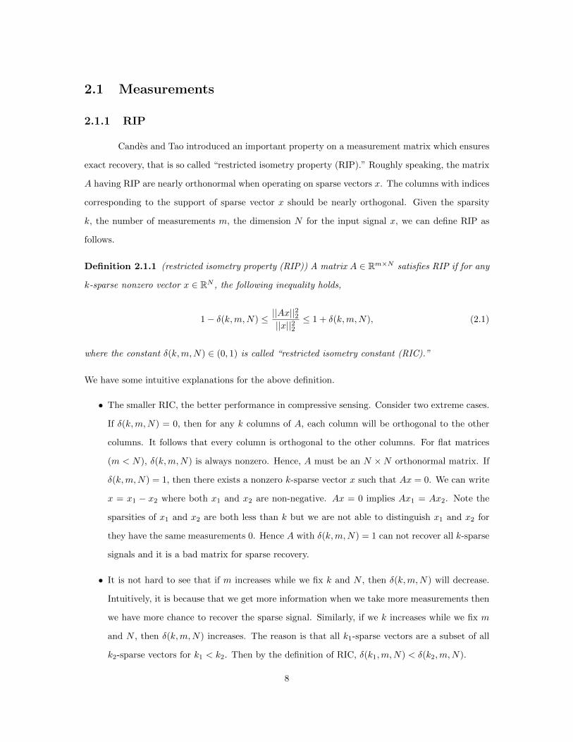
Definition 2.1.1 (restricted isometry property (RIP)) A matrix A ∈ Rm×N satisfies RIP if for any

k-sparse nonzero vector x ∈ RN , the following inequality holds,

1− δ(k,m,N) ≤ ||Ax||22

||x||22≤ 1 + δ(k,m,N), (2.1)

where the constant δ(k,m,N) ∈ (0, 1) is called “restricted isometry constant (RIC).”

We have some intuitive explanations for the above definition.

• The smaller RIC, the better performance in compressive sensing. Consider two extreme cases.

If δ(k,m,N) = 0, then for any k columns of A, each column will be orthogonal to the other

columns. It follows that every column is orthogonal to the other columns. For flat matrices

(m < N), δ(k,m,N) is always nonzero. Hence, A must be an N ×N orthonormal matrix. If

δ(k,m,N) = 1, then there exists a nonzero k-sparse vector x such that Ax = 0. We can write

x = x1 − x2 where both x1 and x2 are non-negative. Ax = 0 implies Ax1 = Ax2. Note the

sparsities of x1 and x2 are both less than k but we are not able to distinguish x1 and x2 for

they have the same measurements 0. Hence A with δ(k,m,N) = 1 can not recover all k-sparse

signals and it is a bad matrix for sparse recovery.

• It is not hard to see that if m increases while we fix k and N , then δ(k,m,N) will decrease.

Intuitively, it is because that we get more information when we take more measurements then

we have more chance to recover the sparse signal. Similarly, if we k increases while we fix m

and N , then δ(k,m,N) increases. The reason is that all k1-sparse vectors are a subset of all

k2-sparse vectors for k1 < k2. Then by the definition of RIC, δ(k1,m,N) < δ(k2,m,N).

8

• Suppose a signal x is supported on T , then y = Ax = A|Tx|T , where x|T (A|T ) is a sub-

vector(sub-matrix) of x(A) restricted on indices T .

We shall see in section 2.2, for both l1-minimization methods and greedy methods, RIP plays an

extremely important role for exact recovery.

Although many papers use RIP, it is important to know that RIP is only a sufficient condition

to ensure exact recovery but not necessary. Another big problem is that testing RIP is NP-hard.

Random matrices (see next chapter) are shown theoretically to have RIPs with a high probability as

long as we have enough measurements. So it is desired to find a property that is not only a necessary

and sufficient condition but also testable. One example is the “Null Space Property (NSP)” in [11].

2.1.2 Measurement Matrices

A nature question is to ask what types of measurement matrices have good RIPs? So far,

most of measurement matrices are constructed using a random processing such as Gaussian matrix,

binary matrix, partial Fourier matrix and incoherent matrix pairs. They have good RIPs with a high

probability as long as we have enough measurements. It turns out that the construction of random

matrices have the advantages in speed, storage as well as the guarantee for exact recovery. But

for implementation, it is still interesting to understand what can be done with purely deterministic

sampling. In the following we will discuss these measurement matrices.

We assume our measurement matrix A ∈ Rm×N . It means the signal has dimension N and

we take m measurements.

• Gaussian matrix. The entries of measurement matrix A are identically sampled from normal

distribution with mean 0 and variance 1/m.

• Binary matrix. The entries of measurement matrix A are identically sampled from symmetric

Bernoulli distribution P (Aij = ±1/√m) = 1/2.

• Partial Fourier matrix. First we define the discrete Fourier matrix F . Its entry [F ]ij at

position (i, j) is

[F ]i,j = e2π√−1(i−1)(j−1)/N .

The partial Fourier matrix A is just taking m rows of the discrete Fourier matrix F . Then we

normalize the columns of A by multiplying 1/√m. Explicitly, let i1, i2, . . . , im be a random

9

subset of 1, 2 . . . , N, then

[A]l,j = [F ]il,j for 1 ≤ l ≤ m.

Remember we assume the measurement matrix should have real entries. So essentially, we are

using the submatrix of discrete Cosine matrix. However, it is a usually it is more convenient to

consider above partial Fourier matrix with complex entries and it won’t affect our problems.

• Incoherent matrix pairs. Define the coherence of the matrix pair (Φ,Ψ) as

µ(Φ,Ψ) =√N max

i,j| 〈φi, ψj〉 |,

where φis are the column vectors of Φ and ψ∗j s are the row vectors of Ψ. The matrix pair (Φ,Ψ)

is said to be incoherent pair if µ(Φ,Ψ) is small. Then A = ΦΨ is our measurement matrix.

Actually, Φ refers to global sensing matrix and Ψ refers to sparse dictionaries (orthonormal

basis).

• Deterministic matrix. For example, [18] and [12].

2.2 Recovery Algorithms

So far, there are many algorithms to solve sparse recovery problems. The two main ap-

proaches are l1-minimization methods and greedy methods. l1-minimization methods relax the

NP-Hard l0-minimization problem to an l1-minimization problem, which can be solved by linear

programming. Although the stability is good, the speed of linear programming is slow as the di-

mension increases. An alternative approach to our sparse recovery problem is via greedy algorithms.

Early greedy algorithms have the advantages in speed but they are bad in stability. Recent greedy

algorithms has bridged the gap between early greedy methods and l1-minimization methods. These

greedy algorithms borrowed the idea of restricted isometry property (RIP) from l1-minimization.

They performed better in both speed and stability.

10

2.2.1 l1-minimization Methods

As we mentioned in section 1.2, the solution to problem (1.4) and problem (1.6) coincide

under some condition on the matrix A. An sufficient condition is exactly the restricted isometry

property mentioned before.

Theorem 2.2.1 (Main Result of l1-minimization Methods [4]) Assume x ∈ RN is a compressible

signal and it has the best k-sparse approximation xs. We are given an m×N measurement matrix

A and a noisy measurement vector y = Ax + e. Suppose x is the solution to the l1-minimization

problem (1.6). If the restricted isometry constant (RIC) of A satisfies δ(2k,m,N) <√

2− 1, then

||x− x||2 ≤ C0 · ||x− xs||1/√k + C1 · ε, (2.2)

for some constants C0 and C1. i.e., problem (1.4) and problem (1.6) are equivalent. The constants

C0 and C1 are typically small. With δ(2k,m,N) = 1/4 for example, C0 ≤ 5.5 and C1 ≤ 6.

2.2.2 Greedy Methods

Three of the state-of-the-art greedy algorithms are compressive sampling matching pursuit

(CoSaMP) [24], subspace pursuit (SP) [10] and iterated hard thresholding (IHT) [2]. Here we discuss

the ideas of these algorithms.

Suppose that we are given a measurement matrix A and a noisy measurement vector y =

Ax+ e and suppose xs is the true best k-sparse approximation of x. Let T denote the support set

of the true sparse vector xs. Although the sparsity k should depend on the signal, here we assume

it is given (prior information). Our goal is to recover x = xs.

Notations. During i-th iteration,

• Estimate: the k-sparse estimate denoted by x[i].

• Support Set: the corresponding support set of x[i] is denoted by T [i].

• Residue: the residue is defined as r[i] = y −Ax[i].

Stopping Criteria: ||r[i]||2 < ε for some small ε > 0.

Algorithm 2.2.2 (CoSaMP)

11

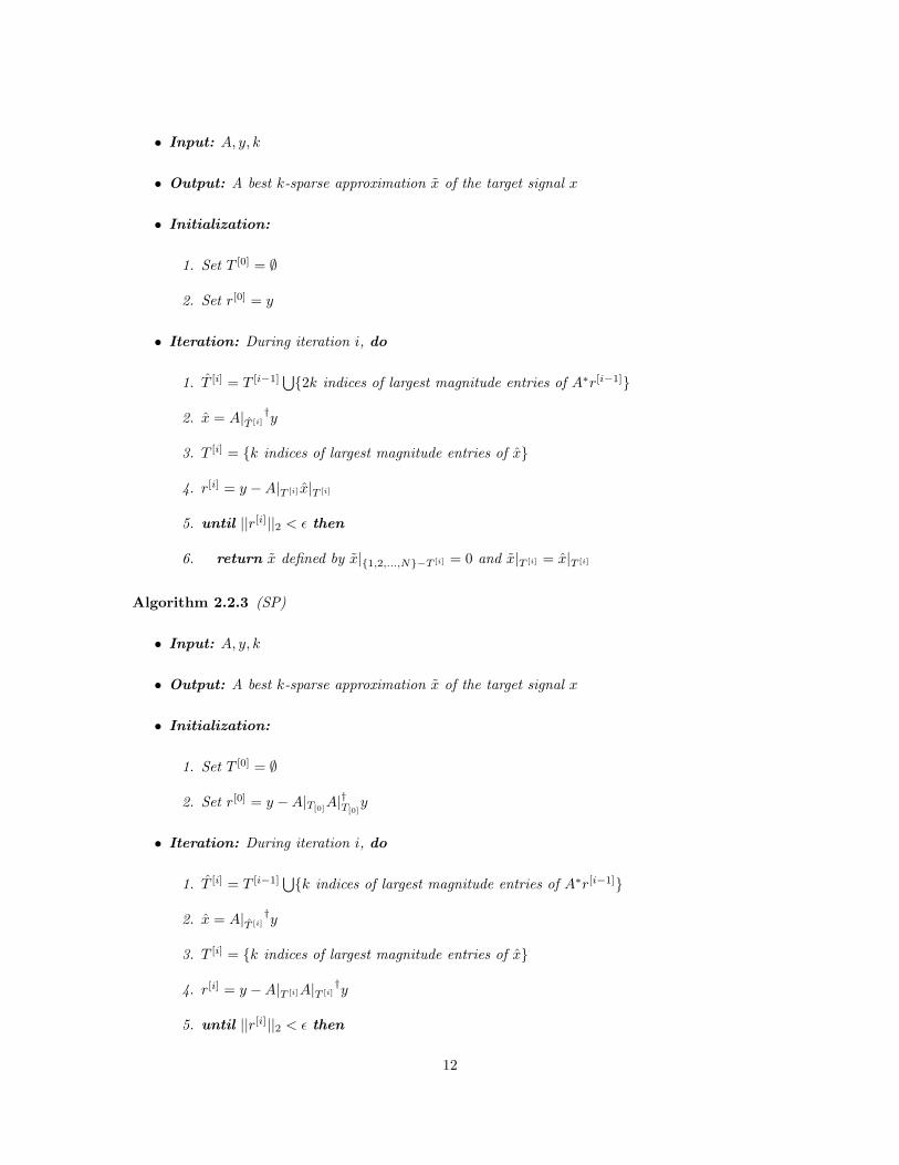
• Input: A, y, k

• Output: A best k-sparse approximation x of the target signal x

• Initialization:

1. Set T [0] = ∅

2. Set r[0] = y

• Iteration: During iteration i, do

1. T [i] = T [i−1]⋃2k indices of largest magnitude entries of A∗r[i−1]

2. x = A|T [i]†y

3. T [i] = k indices of largest magnitude entries of x

4. r[i] = y −A|T [i] x|T [i]

5. until ||r[i]||2 < ε then

6. return x defined by x|1,2,...,N−T [i] = 0 and x|T [i] = x|T [i]

Algorithm 2.2.3 (SP)

• Input: A, y, k

• Output: A best k-sparse approximation x of the target signal x

• Initialization:

1. Set T [0] = ∅

2. Set r[0] = y −A|T[0]A|†T[0]

y

• Iteration: During iteration i, do

1. T [i] = T [i−1]⋃k indices of largest magnitude entries of A∗r[i−1]

2. x = A|T [i]†y

3. T [i] = k indices of largest magnitude entries of x

4. r[i] = y −A|T [i]A|T [i]†y

5. until ||r[i]||2 < ε then

12

6. return x defined by x|1,2,...,N−T [i] = 0 and x|T [i] = A†T [i]y

Algorithm 2.2.4 (IHT)

• Input: A, y, k

• Output: A best k-sparse approximation x of the target signal x

• Initialization:

1. Set x[0] = 0

2. Set T [0] = ∅

3. Set r[0] = y

• Iteration: During iteration i, do

1. x[i] = x[i−1]|T [i−1] + wA∗r[i−1]

2. T [i] = k indices of largest magnitude entries of x[i]

3. r[i] = y −A|T [i]x[i]|T [i]

4. until ||r[i]||2 < ε then

5. return x defined by x|1,2,...,N−T [i] = 0 and x|T [i] = x[i]|T [i]

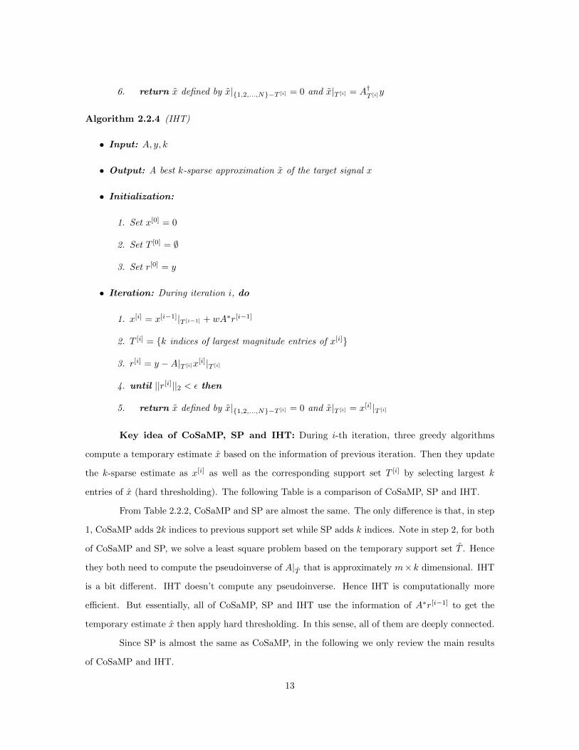
Key idea of CoSaMP, SP and IHT: During i-th iteration, three greedy algorithms

compute a temporary estimate x based on the information of previous iteration. Then they update

the k-sparse estimate as x[i] as well as the corresponding support set T [i] by selecting largest k

entries of x (hard thresholding). The following Table is a comparison of CoSaMP, SP and IHT.

From Table 2.2.2, CoSaMP and SP are almost the same. The only difference is that, in step

1, CoSaMP adds 2k indices to previous support set while SP adds k indices. Note in step 2, for both

of CoSaMP and SP, we solve a least square problem based on the temporary support set T . Hence

they both need to compute the pseudoinverse of A|T that is approximately m× k dimensional. IHT

is a bit different. IHT doesn’t compute any pseudoinverse. Hence IHT is computationally more

efficient. But essentially, all of CoSaMP, SP and IHT use the information of A∗r[i−1] to get the

temporary estimate x then apply hard thresholding. In this sense, all of them are deeply connected.

Since SP is almost the same as CoSaMP, in the following we only review the main results

of CoSaMP and IHT.

13

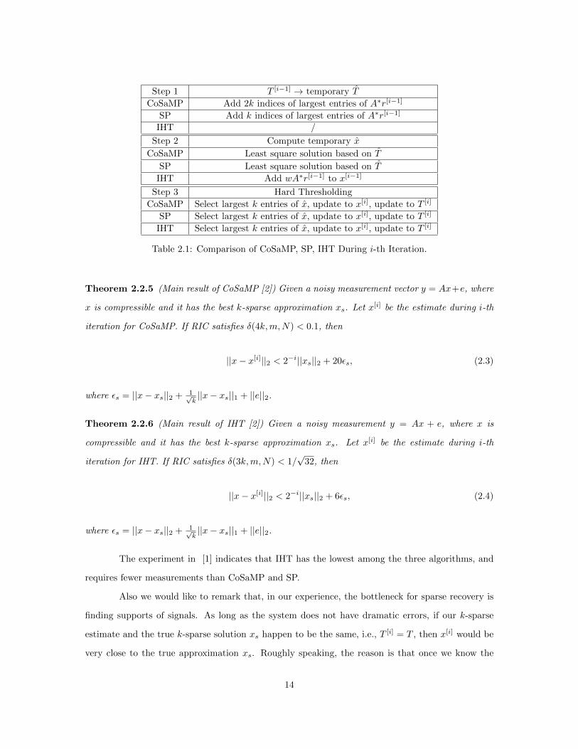
Step 1 T [i−1] → temporary T

CoSaMP Add 2k indices of largest entries of A∗r[i−1]

SP Add k indices of largest entries of A∗r[i−1]

IHT /

Step 2 Compute temporary x

CoSaMP Least square solution based on T

SP Least square solution based on T

IHT Add wA∗r[i−1] to x[i−1]

Step 3 Hard Thresholding

CoSaMP Select largest k entries of x, update to x[i], update to T [i]

SP Select largest k entries of x, update to x[i], update to T [i]

IHT Select largest k entries of x, update to x[i], update to T [i]

Table 2.1: Comparison of CoSaMP, SP, IHT During i-th Iteration.

Theorem 2.2.5 (Main result of CoSaMP [2]) Given a noisy measurement vector y = Ax+e, where

x is compressible and it has the best k-sparse approximation xs. Let x[i] be the estimate during i-th

iteration for CoSaMP. If RIC satisfies δ(4k,m,N) < 0.1, then

||x− x[i]||2 < 2−i||xs||2 + 20εs, (2.3)

where εs = ||x− xs||2 + 1√k||x− xs||1 + ||e||2.

Theorem 2.2.6 (Main result of IHT [2]) Given a noisy measurement y = Ax + e, where x is

compressible and it has the best k-sparse approximation xs. Let x[i] be the estimate during i-th

iteration for IHT. If RIC satisfies δ(3k,m,N) < 1/√

32, then

||x− x[i]||2 < 2−i||xs||2 + 6εs, (2.4)

where εs = ||x− xs||2 + 1√k||x− xs||1 + ||e||2.

The experiment in [1] indicates that IHT has the lowest among the three algorithms, and

requires fewer measurements than CoSaMP and SP.

Also we would like to remark that, in our experience, the bottleneck for sparse recovery is

finding supports of signals. As long as the system does not have dramatic errors, if our k-sparse

estimate and the true k-sparse solution xs happen to be the same, i.e., T [i] = T , then x[i] would be

very close to the true approximation xs. Roughly speaking, the reason is that once we know the

14

support of xs, the system y = Ax + e ≈ Axs becomes over-determined since we have m equations

and only k < m unknown nonzero coefficients of xs. It’s easy to solve the least square problem by

multiplying the pseudoinverse of a sub-matrix of A on y. In other words, if we are able to figure out

the support of xs, then the algorithms immediately converge.

15

Chapter 3

Applications and Extensions of

Compressive Sensing

In practice, there are a lot of sparse or compressible signals. So compressive sensing has a

wide range of applications and extensions. In this chapter, we discuss two direct applications that

are imaging and error correction. Also, we discuss one extension that is robust principle component

analysis.

3.1 Imaging

Let an image be represented by a column vector f ∈ RN . Suppose f is represented by x un-

der certain orthogonal basis such as Fourier basis and wavelets basis. Say the basis is ψ1, ψ2, . . . , ψN .

Then

f = Ψx, (3.1)

where Ψ is an N ×N matrix with waveforms ψi as columns. The entries of x decays significantly

fast if they are sorted by magnitudes. Say x has the best k-sparse approximation xs. Suppose we

have a noisy measurement vector

y = Φf + e, (3.2)

where Φ is an m×N matrix with φ∗i as its rows (see Definition 1.1.2) and e is error.

16

Combine (3.1) and (3.2) and define A = ΦΨ, we get

y = Ax+ e. (3.3)

Hence, the imaging problem is equivalent to the sparse recovery problem 1.1.2. An important

question is: does matrix A = ΦΨ have a good RIP? Recall the definition of coherence of the matrix

pair (Φ,Ψ),

µ(Φ,Ψ) =√N max

i,j| 〈φi, ψj〉 |,

where φi is the column vector of Φ and ψj is the row vector of Ψ. It’s not hard to see that

µ(Φ,Ψ) ∈ [1,√N ]. It’s incoherent if if µ(Φ,Ψ) is close to 1. It’s called maximum incoherent when

µ(Φ,Ψ) = 1. Then we have two typical choices [4]:

1. Φ is spike basis and Ψ is Fourier basis (maximum incoherent);

2. Φ is noiselet and Ψ is wavelets basis [9].

3.2 Error Correction

The error correction problem is modeled as follows [23] [8]. Suppose we have a message

vector f ∈ RK . Let C be the N by K coding matrix, where N > K. Then compute the codeword

vector Cf ∈ RN . The coding matrix is a tall matrix, i.e., the length N of codeword is larger than

the length K of message vector. Let y ∈ RN be received codeword with some error e ∈ RN , say

g = Cf + e. (3.4)

In digital communication, the error vector e ∈ RN has two parts. One is sparse dramatic error

(i.e., some entries in g are highly corrupted) and the other is just small nonsparse random Gaussian

noise. If there are k dramatic errors in the received codeword, then e has k large entries. Suppose

e has the best k-sparse approximation es. For decoding, we are interested in locating the sparse

dramatic errors. In other words, we want to solve for the best k-sparse approximation es. It’s easy

to construct a matrix A ∈ Rm×N of rank m = N −K such that AC = 0. Then (3.4) becomes

Ag = ACf +Ae. (3.5)

17

Let y = Ag. As AC = 0, we have

y = Ae. (3.6)

This is exactly a sparse recovery problem. The error vector e can be found by recovery algorithms

in previous section, provided A is the measurement matrix and y is the measurement vector. For

example we locate the error e by l1-minimization:

mine∈RN

||e||1 s.t. ||y −Ae||2 < ε. (3.7)

3.3 Robust Principle Component Analysis

Robust principle component analysis can be viewed as an extension of compressive sensing.

Suppose we are given an n by n data matrix M which can be decomposed as

M = L0 + S0,

where L0 is a low-rank matrix and S0 a is sparse matrix. Sometimes the data matrix is highly

corrupted. i.e., We have only available a few entries. Let Ω ⊂ [n] × [n] and PΩ be the orthogonal

projection onto the linear space of matrices supported on Ω,

(PΩX)ij =

Xij (i, j) ∈ Ω

0 (i, j) /∈ Ω

We observe

Y = PΩ(L0 + S0) = PΩL0 + S′0. (3.8)

The question is whether it is possible to recover the low-rank component L0 from (3.8). It is showed

in [5] that under certain conditions, L0 can be recovered from (3.8) with high probability by solving

the following problem:

minL,S||L||∗ +

1√n||S||1 s.t. Y = PΩ(L+ S), (3.9)

18

where L has low rank and S is sparse. The nuclear norm ||L||∗ is defined as the sum of all singular

values of L:

||L||∗ =∑

σi(L),

and the l1-norm of S treats the sparse matrix S as a long n× n dimensional vector,

||S||1 =∑|Sij |.

It is assumed that [5]:

1. Ω is uniformly distributed among all subsets of cardinality m obeying m = 0.1n2

2. The incoherence condition on L0. It requires the low-rank matrix M be non-sparse.

The incoherence condition is necessary. The following example is given in [5]. Let M = e1e∗1. Then

M only has one nonzero entry. It is both sparse and low-rank. How can we decide whether it is

low-rank or sparse? In other words, the separation may not be unique. Actually, the incoherence

condition ensures the uniqueness of the solution to (3.9). Also, we can not recover all types of

low-rank matrices. We can only recover those low-rank matrices which satisfy the incoherence

condition.

19

Chapter 4

Generalized Eigenvalues Approach

In this chapter, we starts the case when the measurement matrix is a partial Fourier matrix.

Fourier measurements are important in digital communications, in MRI and probably other applica-

tions. Under this assumption, we show how the recovery problem is related to sparse interpolation.

In the first section, we discuss sparse interpolation problem via generalized eigenvalues method. In

the second section, we modify the generalized eigenvalues method by taking more than 2k measure-

ments and apply it to compressive sensing. We call our new algorithm generalized eigenvalues (GE).

Then we compare GE with Iterated Hard Thresholding (IHT). The result indicates GE performs

much better if the number of Fourier measurements is small while IHT is better when the number

of measurements is very large. Finally, our experiments indicate that GE may be improved by using

adaptive measurements.

4.1 Generalized Eigenvalues for Sparse Interpolation with

m = 2k

4.1.1 Sparse Interpolation

Problem 4.1.1 (Sparse Interpolation) Suppose we are given a black box for a k-sparse univariate

polynomial f ∈ R[t]

f(t) =

k∑j=1

cjtdj ,

20

where c1, c2, . . . , ct ∈ R and d1, d2, . . . , dk ∈ Z≥0. We assume that the degree of the polynomial is

less than N ,

0 ≤ d1 < d2 < · · · < dk ≤ N − 1.

Evaluating

y1 = f(ν1), y2 = f(ν2), y3 = f(ν3), . . . , ym = f(νm) (4.1)

at our own choice of points ν1, ν2, . . . , νm ∈ C, where m = O(k), we want to determine the exponents

d1, d2, . . . , dk and the coefficients c1, c2, . . . , ck.

4.1.2 Generalized Eigenvalues

Let ω0 be the N -th root of unity,

ω0 = e2πiN .

We evaluate at 1, ω0, ω20 , . . . , ω

2k−10 to get our first 2k Fourier coefficients,

y1 = f(1), y2 = f(ω0), y3 = f(ω20), . . . , y2k = f(ω2k−1

0 ). (4.2)

Let

b1 = ωd10 , , . . . , bk = ωdk0 . (4.3)

If we write the evaluation process in the form of matrix multiplication, then (4.2) is equivalent to

y =

y1

y2

...

y2k

=

1 1 . . . 1

b1 b2 . . . bk...

.... . .

...

b2k−11 b2k−1

2 . . . b2k−1k

c1

c2...

ck

. (4.4)

21

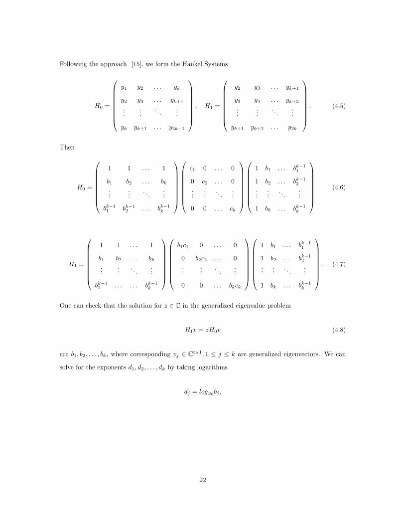
Following the approach [15], we form the Hankel Systems

H0 =

y1 y2 . . . yk

y2 y3 . . . yk+1

......

. . ....

yk yk+1 . . . y2k−1

, H1 =

y2 y3 . . . yk+1

y3 y4 . . . yk+2

......

. . ....

yk+1 yk+2 . . . y2k

. (4.5)

Then

H0 =

1 1 . . . 1

b1 b2 . . . bk...

.... . .

...

bk−11 bk−1

2 . . . bk−1k

c1 0 . . . 0

0 c2 . . . 0

......

. . ....

0 0 . . . ck

1 b1 . . . bk−11

1 b2 . . . bk−12

......

. . ....

1 bk . . . bk−1k

(4.6)

H1 =

1 1 . . . 1

b1 b2 . . . bk...

.... . .

...

bk−11 . . . . . . bk−1

k

b1c1 0 . . . 0

0 b2c2 . . . 0

......

. . ....

0 0 . . . bkck

1 b1 . . . bk−11

1 b2 . . . bk−12

......

. . ....

1 bk . . . bk−1k

. (4.7)

One can check that the solution for z ∈ C in the generalized eigenvalue problem

H1v = zH0v (4.8)

are b1, b2, . . . , bk, where corresponding vj ∈ Ct×1, 1 ≤ j ≤ k are generalized eigenvectors. We can

solve for the exponents d1, d2, . . . , dk by taking logarithms

dj = logω0bj ,

22

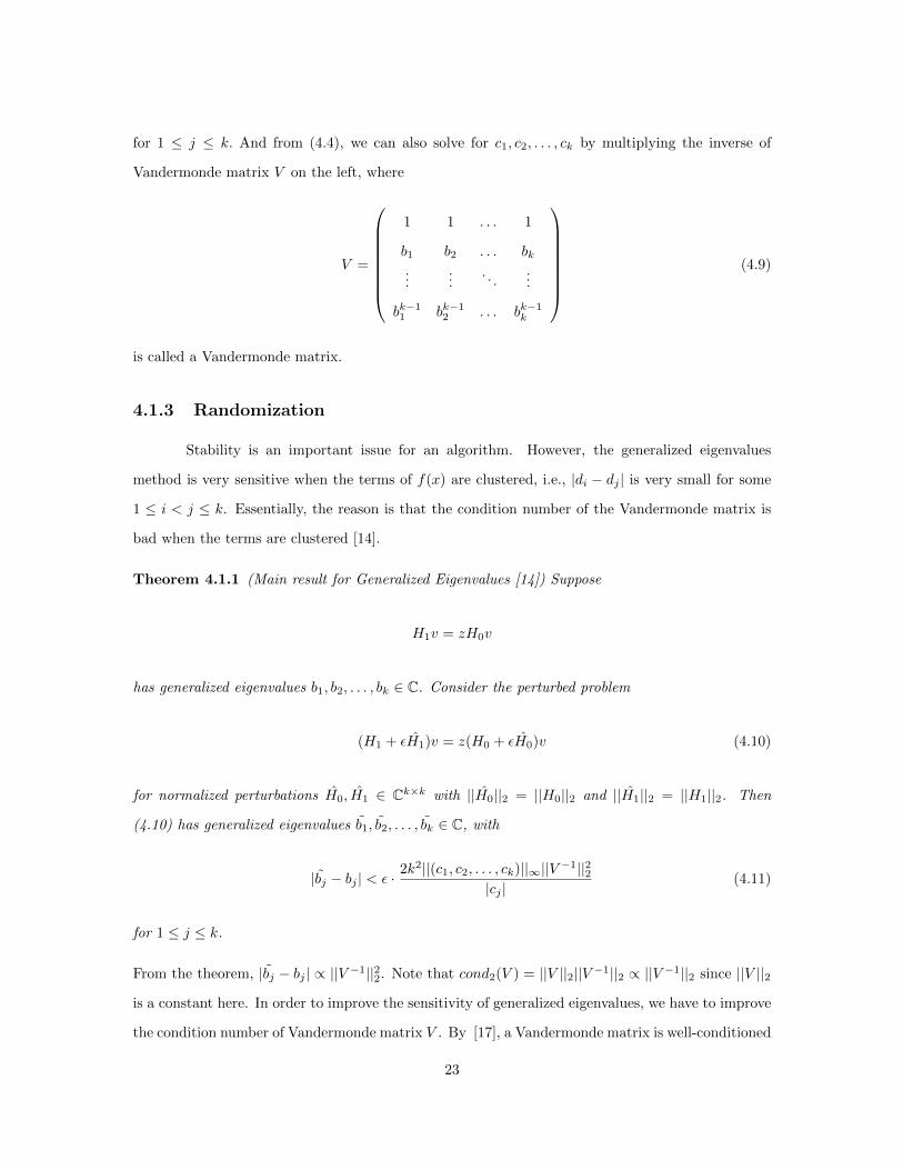
for 1 ≤ j ≤ k. And from (4.4), we can also solve for c1, c2, . . . , ck by multiplying the inverse of

Vandermonde matrix V on the left, where

V =

1 1 . . . 1

b1 b2 . . . bk...

.... . .

...

bk−11 bk−1

2 . . . bk−1k

(4.9)

is called a Vandermonde matrix.

4.1.3 Randomization

Stability is an important issue for an algorithm. However, the generalized eigenvalues

method is very sensitive when the terms of f(x) are clustered, i.e., |di − dj | is very small for some

1 ≤ i < j ≤ k. Essentially, the reason is that the condition number of the Vandermonde matrix is

bad when the terms are clustered [14].

Theorem 4.1.1 (Main result for Generalized Eigenvalues [14]) Suppose

H1v = zH0v

has generalized eigenvalues b1, b2, . . . , bk ∈ C. Consider the perturbed problem

(H1 + εH1)v = z(H0 + εH0)v (4.10)

for normalized perturbations H0, H1 ∈ Ck×k with ||H0||2 = ||H0||2 and ||H1||2 = ||H1||2. Then

(4.10) has generalized eigenvalues b1, b2, . . . , bk ∈ C, with

|bj − bj | < ε · 2k2||(c1, c2, . . . , ck)||∞||V −1||22|cj |

(4.11)

for 1 ≤ j ≤ k.

From the theorem, |bj − bj | ∝ ||V −1||22. Note that cond2(V ) = ||V ||2||V −1||2 ∝ ||V −1||2 since ||V ||2

is a constant here. In order to improve the sensitivity of generalized eigenvalues, we have to improve

the condition number of Vandermonde matrix V . By [17], a Vandermonde matrix is well-conditioned

23

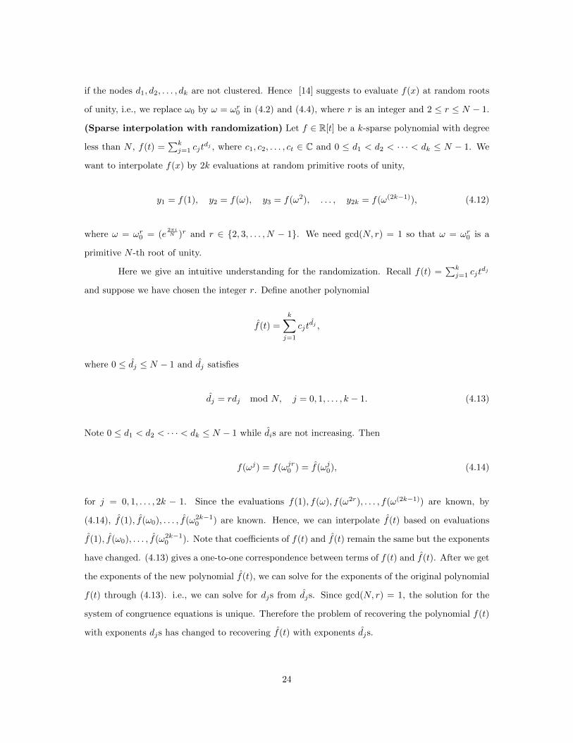
if the nodes d1, d2, . . . , dk are not clustered. Hence [14] suggests to evaluate f(x) at random roots

of unity, i.e., we replace ω0 by ω = ωr0 in (4.2) and (4.4), where r is an integer and 2 ≤ r ≤ N − 1.

(Sparse interpolation with randomization) Let f ∈ R[t] be a k-sparse polynomial with degree

less than N , f(t) =∑kj=1 cjt

dj , where c1, c2, . . . , ct ∈ C and 0 ≤ d1 < d2 < · · · < dk ≤ N − 1. We

want to interpolate f(x) by 2k evaluations at random primitive roots of unity,

y1 = f(1), y2 = f(ω), y3 = f(ω2), . . . , y2k = f(ω(2k−1)), (4.12)

where ω = ωr0 = (e2πiN )r and r ∈ 2, 3, . . . , N − 1. We need gcd(N, r) = 1 so that ω = ωr0 is a

primitive N -th root of unity.

Here we give an intuitive understanding for the randomization. Recall f(t) =∑kj=1 cjt

dj

and suppose we have chosen the integer r. Define another polynomial

f(t) =

k∑j=1

cjtdj ,

where 0 ≤ dj ≤ N − 1 and dj satisfies

dj = rdj mod N, j = 0, 1, . . . , k − 1. (4.13)

Note 0 ≤ d1 < d2 < · · · < dk ≤ N − 1 while dis are not increasing. Then

f(ωj) = f(ωjr0 ) = f(ωj0), (4.14)

for j = 0, 1, . . . , 2k − 1. Since the evaluations f(1), f(ω), f(ω2r), . . . , f(ω(2k−1)) are known, by

(4.14), f(1), f(ω0), . . . , f(ω2k−10 ) are known. Hence, we can interpolate f(t) based on evaluations

f(1), f(ω0), . . . , f(ω2k−10 ). Note that coefficients of f(t) and f(t) remain the same but the exponents

have changed. (4.13) gives a one-to-one correspondence between terms of f(t) and f(t). After we get

the exponents of the new polynomial f(t), we can solve for the exponents of the original polynomial

f(t) through (4.13). i.e., we can solve for djs from djs. Since gcd(N, r) = 1, the solution for the

system of congruence equations is unique. Therefore the problem of recovering the polynomial f(t)

with exponents djs has changed to recovering f(t) with exponents djs.

24

Let ciedi and cje

dj be any two terms of f(t). Define the distance for the two terms as

dij = min|di − dj |, N − |di − dj |. For example, if di = 0 and dj = N − 1, then dij = 1 by the

definition and we consider them as clustered terms. Let ∆ be the minimal distance for terms of f(t),

∆ = mini,j

dij .

Then f(t) has clustered terms if ∆ is small.

Similarly, let ciedi and cje

dj be any two terms of f(t). Define their distance as dij =

min|di − dj |, N − |di − dj |. Let ∆ be the minimal distance for terms of f(t),

∆ = mini,j

dij .

As we mentioned before, the generalized eigenvalues method is especially sensitive in the

case that the polynomial has clustered terms (i.e., when ∆ is very small). Hence, if ∆ happens to

be small, then we are supposed to choose a proper integer r to increase ∆ as much as possible. But

the problem is that we don’t have any prior information about how the terms are clustered.

If we randomly choose an integer r, how likely ∆ is not small? We have the following

theorem.

Theorem 4.1.2 [14] Let r be chosen uniformly and randomly from 1, 2, . . . , N − 1. Then with

probability at least 1/2,

∆ > bNk2c.

4.1.4 Relationship between Sparse Interpolation and Compressive Sens-

ing

In this section, we claim sparse interpolation problem is a special sparse recovery problem

in compressive sensing. The evaluations in sparse interpolation can actually be viewed as Fourier

measurements in compressive sensing.

For sparse interpolation (4.1), we want to determine the k-sparse polynomial

f(t) =

k∑j=1

cjtdj ∈ R[t]

25

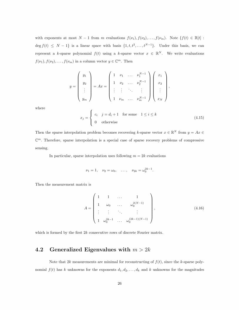
with exponents at most N − 1 from m evaluations f(ν1), f(ν2), . . . , f(νm). Note f(t) ∈ R[t] :

deg f(t) ≤ N − 1 is a linear space with basis 1, t, t2, . . . , tN−1. Under this basis, we can

represent a k-sparse polynomial f(t) using a k-sparse vector x ∈ RN . We write evaluations

f(ν1), f(ν2), . . . , f(νm) in a column vector y ∈ Cm. Then

y =

y1

y2

...

ym

= Ax =

1 ν1 . . . νN−11

1 ν2 . . . νN−12

......

. . ....

1 νm . . . νN−1m

x1

x2

...

xN

,

where

xj =

ci j = di + 1 for some 1 ≤ i ≤ k

0 otherwise(4.15)

Then the sparse interpolation problem becomes recovering k-sparse vector x ∈ RN from y = Ax ∈

Cm. Therefore, sparse interpolation is a special case of sparse recovery problems of compressive

sensing.

In particular, sparse interpolation uses following m = 2k evaluations

ν1 = 1, ν2 = ω0, . . . , ν2k = ω2k−10 .

Then the measurement matrix is

A =

1 1 . . . 1

1 ω0 . . . ω2(N−1)0

......

. . ....

1 ω2k−10 . . . ω

(2k−1)(N−1)0

, (4.16)

which is formed by the first 2k consecutive rows of discrete Fourier matrix.

4.2 Generalized Eigenvalues with m > 2k

Note that 2k measurements are minimal for reconstructing of f(t), since the k-sparse poly-

nomial f(t) has k unknowns for the exponents d1, d2, . . . , dk and k unknowns for the magnitudes

26

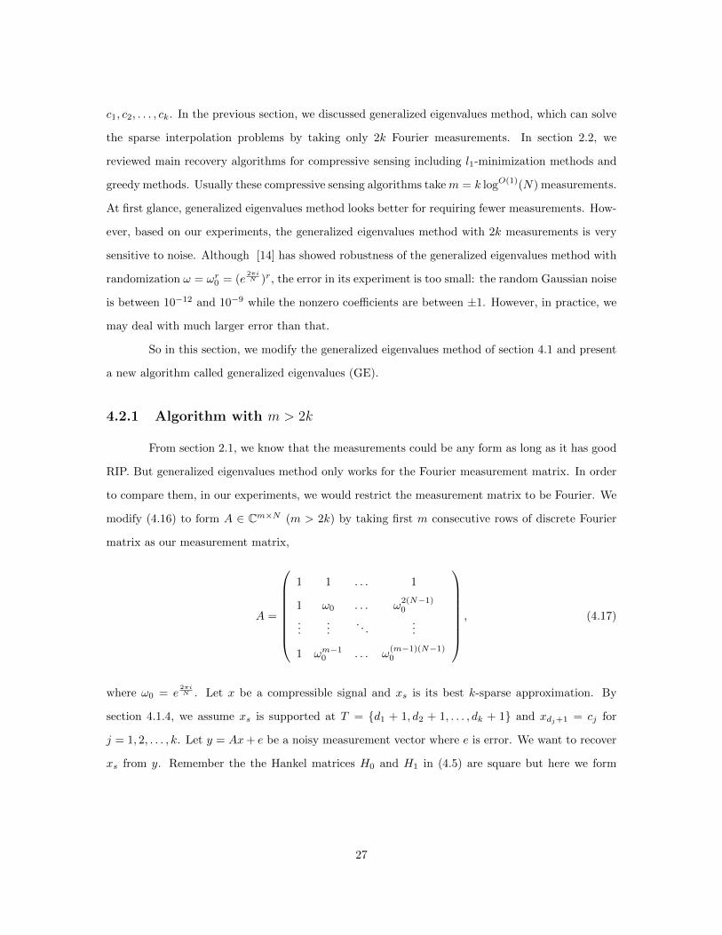
c1, c2, . . . , ck. In the previous section, we discussed generalized eigenvalues method, which can solve

the sparse interpolation problems by taking only 2k Fourier measurements. In section 2.2, we

reviewed main recovery algorithms for compressive sensing including l1-minimization methods and

greedy methods. Usually these compressive sensing algorithms takem = k logO(1)(N) measurements.

At first glance, generalized eigenvalues method looks better for requiring fewer measurements. How-

ever, based on our experiments, the generalized eigenvalues method with 2k measurements is very

sensitive to noise. Although [14] has showed robustness of the generalized eigenvalues method with

randomization ω = ωr0 = (e2πiN )r, the error in its experiment is too small: the random Gaussian noise

is between 10−12 and 10−9 while the nonzero coefficients are between ±1. However, in practice, we

may deal with much larger error than that.

So in this section, we modify the generalized eigenvalues method of section 4.1 and present

a new algorithm called generalized eigenvalues (GE).

4.2.1 Algorithm with m > 2k

From section 2.1, we know that the measurements could be any form as long as it has good

RIP. But generalized eigenvalues method only works for the Fourier measurement matrix. In order

to compare them, in our experiments, we would restrict the measurement matrix to be Fourier. We

modify (4.16) to form A ∈ Cm×N (m > 2k) by taking first m consecutive rows of discrete Fourier

matrix as our measurement matrix,

A =

1 1 . . . 1

1 ω0 . . . ω2(N−1)0

......

. . ....

1 ωm−10 . . . ω

(m−1)(N−1)0

, (4.17)

where ω0 = e2πiN . Let x be a compressible signal and xs is its best k-sparse approximation. By

section 4.1.4, we assume xs is supported at T = d1 + 1, d2 + 1, . . . , dk + 1 and xdj+1 = cj for

j = 1, 2, . . . , k. Let y = Ax+ e be a noisy measurement vector where e is error. We want to recover

xs from y. Remember the the Hankel matrices H0 and H1 in (4.5) are square but here we form

27

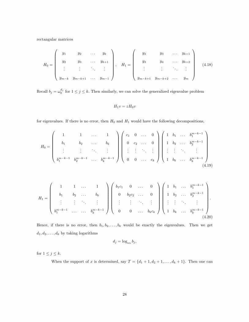
rectangular matrices

H0 =

y1 y2 . . . yk

y2 y3 . . . yk+1

......

. . ....

ym−k ym−k+1 . . . ym−1

, H1 =

y2 y3 . . . yk+1

y3 y4 . . . yk+2

......

. . ....

ym−k+1 ym−k+2 . . . ym

(4.18)

Recall bj = ωdj0 for 1 ≤ j ≤ k. Then similarly, we can solve the generalized eigenvalue problem

H1v = zH0v

for eigenvalues. If there is no error, then H0 and H1 would have the following decompositions,

H0 =

1 1 . . . 1

b1 b2 . . . bk...

.... . .

...

bm−k−11 bm−k−1

2 . . . bm−k−1k

c1 0 . . . 0

0 c2 . . . 0

......

. . ....

0 0 . . . ck

1 b1 . . . bm−k−11

1 b2 . . . bm−k−12

......

. . ....

1 bk . . . bm−k−1k

(4.19)

H1 =

1 1 . . . 1

b1 b2 . . . bk...

.... . .

...

bm−k−11 . . . . . . bm−k−1

k

b1c1 0 . . . 0

0 b2c2 . . . 0

......

. . ....

0 0 . . . bkck

1 b1 . . . bm−k−11

1 b2 . . . bm−k−12

......

. . ....

1 bk . . . bm−k−1k

.

(4.20)

Hence, if there is no error, then b1, b2, . . . , bk would be exactly the eigenvalues. Then we get

d1, d2, . . . , dk by taking logarithms

dj = logω0bj ,

for 1 ≤ j ≤ k.

When the support of x is determined, say T = d1 + 1, d2 + 1, . . . , dk + 1. Then one can

28

solve for coefficients c1, c2, . . . , ck. Let V be the rectangular Vandermonde matrix,

V =

1 1 . . . 1

b1 b2 . . . bk...

.... . .

...

bm−k−11 bm−k−1

2 . . . bm−k−1k

(4.21)

Note V = A|T and x|T = xs|T = (c1, c2, . . . , ck)t, then

y = Ax+ e ≈ Ax ≈ Axs = A|Txs|T = V · (c1, c2, . . . , ck)t

The system is over determined since we have m equations and only k < m unknowns. Hence it’s

easy to solve for cjs as follows:

(c1, c2, . . . , ck)t = V †y, (4.22)

where V † is the pseudoinverse of V . Finally reconstruct the signal using (4.15).

4.2.2 Determining the Sparsity

Greedy algorithms in section 2.2 use sparsity k as an input. However, k is usually unknown

and it has to be determined. In some paper, they use estimates. For example, in [24], they take

k ≈ m/(2 logN). One of the advantages of our generalized eigenvalues method is that we are able to

determine the sparsity from the rank of a series of square Hankel matrices. Suppose from a k-sparse

signal x we have measured y1, y2, . . . , ym which are not noisy. Let 1 ≤ j ≤ bm2 c. We consider the

rank of following square Hankel matrix,

H [j] =

y1 y2 . . . yj

y2 y3 . . . yj+1

......

. . ....

yj yj+1 . . . y2j−1

.

29

If j ≥ k, then H [j] has the following decomposition

H [j] =

1 1 . . . 1

b1 b2 . . . bk...

.... . .

...

bj−11 bj−1

2 . . . bj−1k

c1 0 . . . 0

0 c2 . . . 0

......

. . ....

0 0 . . . ck

1 b1 . . . bj−11

1 b2 . . . bj−12

......

. . ....

1 bk . . . bj−1k

Hence, if j ≥ k, the rank of H [j] is equal to the sparsity k. If j < k, then the rank of H [j] is obviously

less than k. Therefore, we determine the sparsity by computing the ranks of H [1], H [2], . . . until they

remain a finite integer k. Then integer k is the sparsity. Actually, let j = bm2 c. If m is large enough,

then j > k. We can determine the sparsity k by only computing the rank of H [j].

However, if the measurement vector y is noisy, then it would be a bit harder to determine

the rank of a singular matrix since it usually becomes a full-rank matrix. In this case, we determine

an approximate rank as follows. Suppose the eigenvalues of H [j] are

λ1 ≥ λ2 ≥ · · · ≥ λk ≥ · · · ≥ λj ≥ 0.

As long as their is no dramatic error,

λ1, λ2, . . . , λk ≈ c1, c2, . . . , ck, λk+1 ≈ 0, . . . , λj ≈ 0.

Let gj , j = 1, 2, . . . , j − 1 be the“gaps” between those eigenvalues,

g1 =λ1

λ2, g2 =

λ2

λ3, . . . gj−1 =

λj−1

λj

If the error is a bit large, a safe way is to choose a larger integer k as the sparsity. A larger sparsity

k won’t affect the result of our generalized eigenvalues method. Also, after we have determined the

sparsity k, we replace k by 2k and then solve for d1, d2, . . . , d2k by generalized eigenvalues method.

Since djs are supposed to integer, from them we select d1, d2, . . . , dk with smallest imaginary parts.

4.2.3 Algorithm

Now we present our algorithm of generalized eigenvalues (GE)

30

Algorithm 4.2.1 (GE)

• Input: A measurement vector y ∈ Cm, the signal dimension N .

• Output: support and corresponding coefficients (c1, d1 + 1), (c2, d2 + 1), . . . , (ck, dk + 1).

1. Determine an approximate sparsity k. Let j = bm2 c, construct H [j] and compute

its rank using the method of section 4.2.2. Set the sparsity k as an integer that is slightly

larger than the rank of H [j].

2. Construct Hankel Systems H0 and H1. Use the k from step 1 to form H0, H1 ∈

C(m−2k)×2k as in (4.18) where k is replaced by 2k.

3. Solve a generalized eigenvalue problem. Solve 2k generalized eigenvalues b1, b2, . . . , b2k

from H1v = zH0v.

4. Take logarithms. dj = logω0bj , where ω0 = e

2πiN .

5. Determine support. From above d1, d2, . . . , d2k, select d1, d2, . . . , dk with smallest imag-

inary parts. Set d1 + 1, d2 + 1, . . . , dk + 1 as the support.

6. Determine coefficients. Construct a rectangular Vandermonde matrix V as in (4.21)

and solve for nonzero coefficients c1, c2, . . . , ck by (4.22).

4.2.4 GE vs IHT

By section 2.2.2, the greedy algorithms (CosaMP, SP, IHT) are fast and have good stability.

And IHT is the best one among them because IHT has the lowest computational cost, and requires

fewer measurements than CoSaMP and SP [1]. Hence, in this section, we compare our generalized

eigenvalues method (GE) with Iterated Hard Thresholding (IHT).

We randomly generate a k-sparse signal x of length N = 1009. We first pick k random

positions as the support set of x and for each position, we set the corresponding entry of x via

uniform distribution U(−1, 1). Then for GE, we take first m consecutive rows of discrete Fourier

matrix as our measurement matrix. For IHT, we randomly select m rows from discrete Fourier

matrix and then normalized the columns. In Figure (a), we add complex Gaussian noise of level

10−5 on the measurements. In Figure (b), we add complex Gaussian noise of level 10−4 on the

measurement. In Figure (c), we add complex Gaussian noise of level 10−3 on the measurements.

And for all Figure (a), (b) and (c), the x-axis is the number of measurements m, which varies from

31

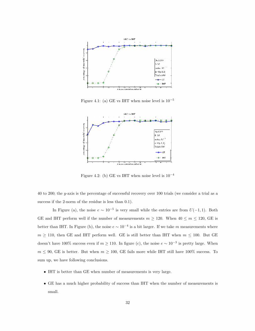
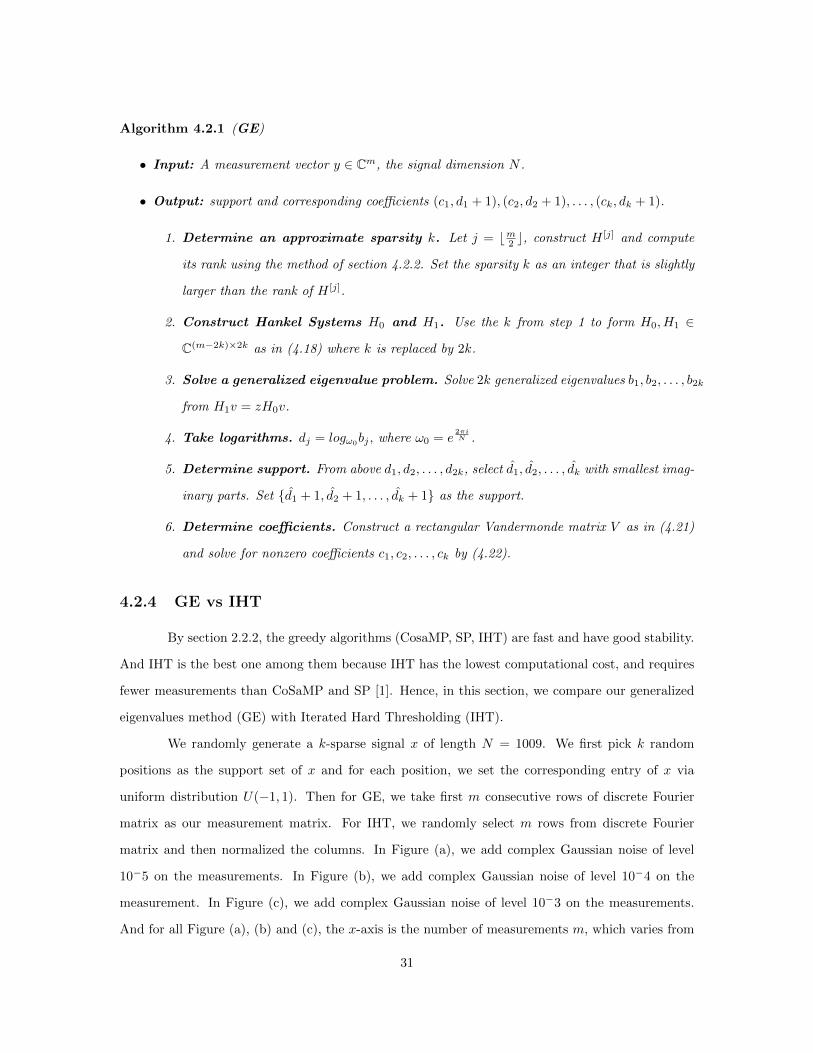
Figure 4.1: (a) GE vs IHT when noise level is 10−5

Figure 4.2: (b) GE vs IHT when noise level is 10−4

40 to 200; the y-axis is the percentage of successful recovery over 100 trials (we consider a trial as a

success if the 2-norm of the residue is less than 0.1).

In Figure (a), the noise e ∼ 10−5 is very small while the entries are from U(−1, 1). Both

GE and IHT perform well if the number of measurements m ≥ 120. When 40 ≤ m ≤ 120, GE is

better than IHT. In Figure (b), the noise e ∼ 10−4 is a bit larger. If we take m measurements where

m ≥ 110, then GE and IHT perform well. GE is still better than IHT when m ≤ 100. But GE

doesn’t have 100% success even if m ≥ 110. In figure (c), the noise e ∼ 10−3 is pretty large. When

m ≤ 90, GE is better. But when m ≥ 100, GE fails more while IHT still have 100% success. To

sum up, we have following conclusions.

• IHT is better than GE when number of measurements is very large.

• GE has a much higher probability of success than IHT when the number of measurements is

small.

32

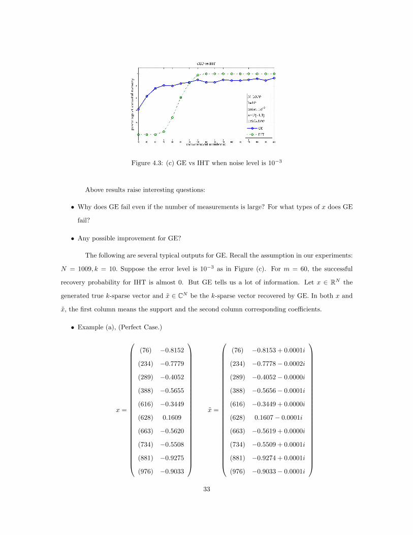
Figure 4.3: (c) GE vs IHT when noise level is 10−3

Above results raise interesting questions:

• Why does GE fail even if the number of measurements is large? For what types of x does GE

fail?

• Any possible improvement for GE?

The following are several typical outputs for GE. Recall the assumption in our experiments:

N = 1009, k = 10. Suppose the error level is 10−3 as in Figure (c). For m = 60, the successful

recovery probability for IHT is almost 0. But GE tells us a lot of information. Let x ∈ RN the

generated true k-sparse vector and x ∈ CN be the k-sparse vector recovered by GE. In both x and

x, the first column means the support and the second column corresponding coefficients.

• Example (a), (Perfect Case.)

x =

(76) −0.8152

(234) −0.7779

(289) −0.4052

(388) −0.5655

(616) −0.3449

(628) 0.1609

(663) −0.5620

(734) −0.5508

(881) −0.9275

(976) −0.9033

x =

(76) −0.8153 + 0.0001i

(234) −0.7778− 0.0002i

(289) −0.4052− 0.0000i

(388) −0.5656− 0.0001i

(616) −0.3449 + 0.0000i

(628) 0.1607− 0.0001i

(663) −0.5619 + 0.0000i

(734) −0.5509 + 0.0001i

(881) −0.9274 + 0.0001i

(976) −0.9033− 0.0001i

33

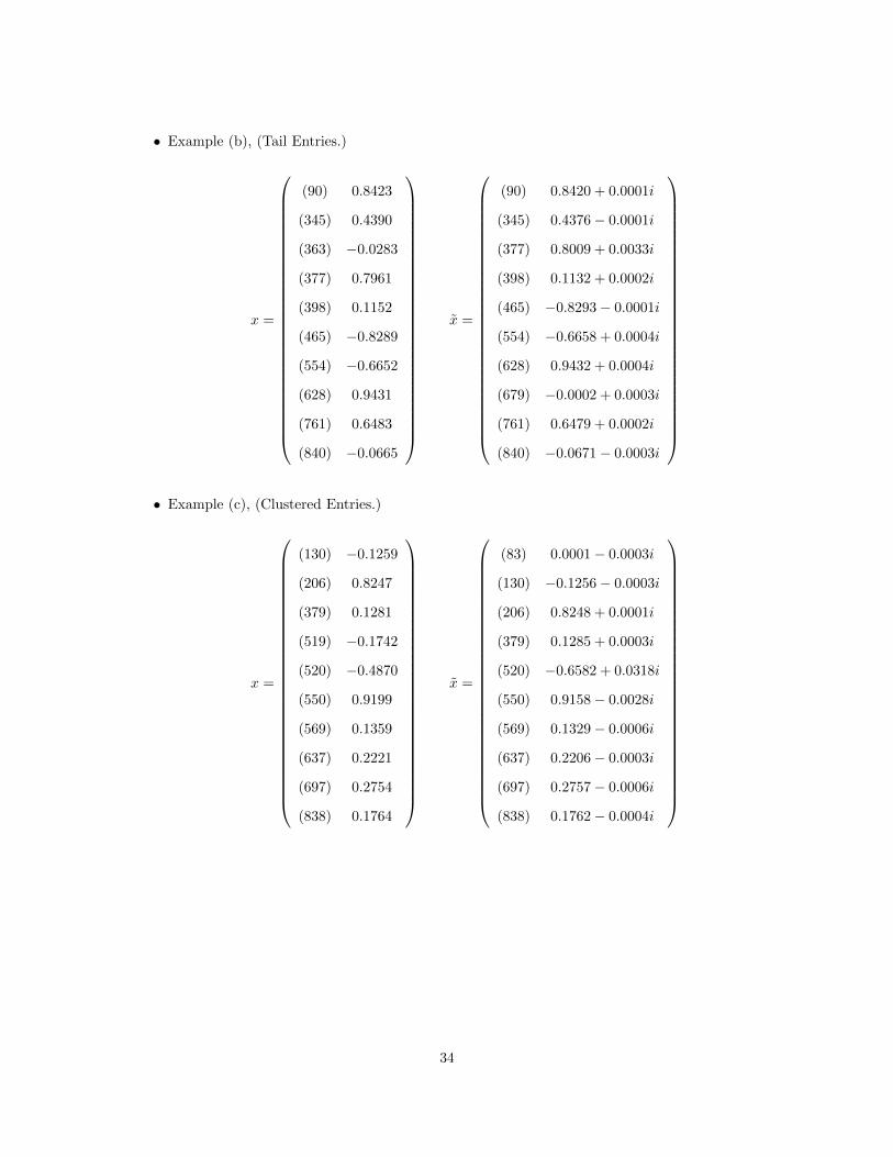
• Example (b), (Tail Entries.)

x =

(90) 0.8423

(345) 0.4390

(363) −0.0283

(377) 0.7961

(398) 0.1152

(465) −0.8289

(554) −0.6652

(628) 0.9431

(761) 0.6483

(840) −0.0665

x =

(90) 0.8420 + 0.0001i

(345) 0.4376− 0.0001i

(377) 0.8009 + 0.0033i

(398) 0.1132 + 0.0002i

(465) −0.8293− 0.0001i

(554) −0.6658 + 0.0004i

(628) 0.9432 + 0.0004i

(679) −0.0002 + 0.0003i

(761) 0.6479 + 0.0002i

(840) −0.0671− 0.0003i

• Example (c), (Clustered Entries.)

x =

(130) −0.1259

(206) 0.8247

(379) 0.1281

(519) −0.1742

(520) −0.4870

(550) 0.9199

(569) 0.1359

(637) 0.2221

(697) 0.2754

(838) 0.1764

x =

(83) 0.0001− 0.0003i

(130) −0.1256− 0.0003i

(206) 0.8248 + 0.0001i

(379) 0.1285 + 0.0003i

(520) −0.6582 + 0.0318i

(550) 0.9158− 0.0028i

(569) 0.1329− 0.0006i

(637) 0.2206− 0.0003i

(697) 0.2757− 0.0006i

(838) 0.1762− 0.0004i

34

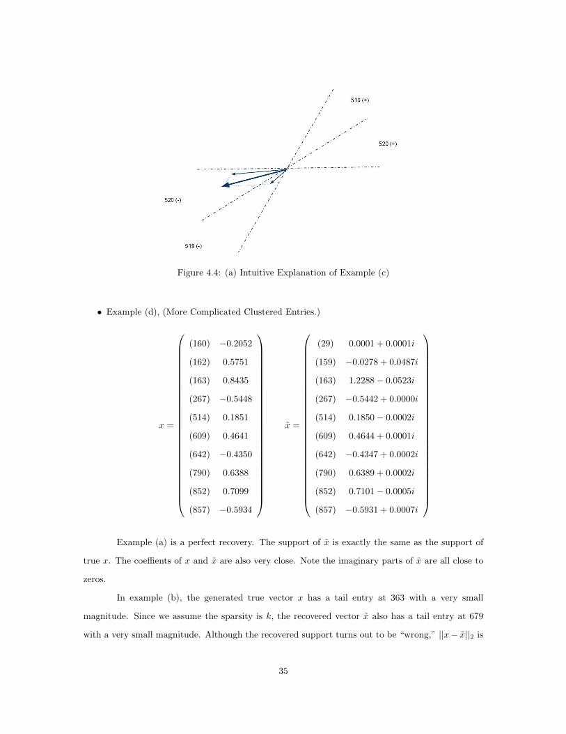
Figure 4.4: (a) Intuitive Explanation of Example (c)

• Example (d), (More Complicated Clustered Entries.)

x =

(160) −0.2052

(162) 0.5751

(163) 0.8435

(267) −0.5448

(514) 0.1851

(609) 0.4641

(642) −0.4350

(790) 0.6388

(852) 0.7099

(857) −0.5934

x =

(29) 0.0001 + 0.0001i

(159) −0.0278 + 0.0487i

(163) 1.2288− 0.0523i

(267) −0.5442 + 0.0000i

(514) 0.1850− 0.0002i

(609) 0.4644 + 0.0001i

(642) −0.4347 + 0.0002i

(790) 0.6389 + 0.0002i

(852) 0.7101− 0.0005i

(857) −0.5931 + 0.0007i

Example (a) is a perfect recovery. The support of x is exactly the same as the support of

true x. The coeffients of x and x are also very close. Note the imaginary parts of x are all close to

zeros.

In example (b), the generated true vector x has a tail entry at 363 with a very small

magnitude. Since we assume the sparsity is k, the recovered vector x also has a tail entry at 679

with a very small magnitude. Although the recovered support turns out to be “wrong,” ||x− x||2 is

35

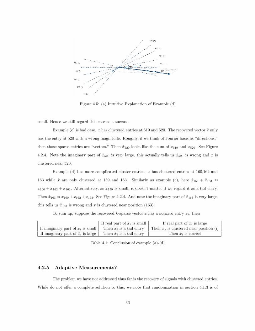
Figure 4.5: (a) Intuitive Explanation of Example (d)

small. Hence we still regard this case as a succuss.

Example (c) is bad case. x has clustered entries at 519 and 520. The recovered vector x only

has the entry at 520 with a wrong magnitude. Roughly, if we think of Fourier basis as “directions,”

then those sparse entries are “vectors.” Then x520 looks like the sum of x519 and x520. See Figure

4.2.4. Note the imaginary part of x520 is very large, this actually tells us x520 is wrong and x is

clustered near 520.

Example (d) has more complicated cluster entries. x has clustered entries at 160,162 and

163 while x are only clustered at 159 and 163. Similarly as example (c), here x159 + x163 ≈

x160 + x162 + x163. Alternatively, as x159 is small, it doesn’t matter if we regard it as a tail entry.

Then x163 ≈ x160 +x162 +x163. See Figure 4.2.4. And note the imaginary part of x163 is very large,

this tells us x163 is wrong and x is clustered near position (163)!

To sum up, suppose the recovered k-sparse vector x has a nonzero entry xi, then

If real part of xi is small If real part of xi is largeIf imaginary part of xi is small Then xi is a tail entry Then xs is clustered near position (i)If imaginary part of xi is large Then xi is a tail entry Then xi is correct

Table 4.1: Conclusion of example (a)-(d)

4.2.5 Adaptive Measurements?

The problem we have not addressed thus far is the recovery of signals with clustered entries.

While do not offer a complete solution to this, we note that randomization in section 4.1.3 is of

36

potential help. Let x be the recovered vector using GE algorithm. Suppose xd1+1, xd2+1, . . . , xdj+1

have both large real parts and imaginary parts, where d1 + 1, d2 + 1, . . . , dj + 1 ⊆ [C −Θ, C + Θ].

Then by Table 4.2.4, xs has clustered entries within [C − γΘ, C + γΘ] for some γ > 1. Although we

known where the the entries are clustered, we are not able to separate them using current measure-

ments. Recall the idea of randomization in section 4.1.3, if we do another round of measurements

with randomization, then d1+1, d2+1, . . . , dj+1 becomes rd1+1, rd2+1, . . . , rdj+1( mod N).

And it’s possible that these clustered entries xd1+1, xd2+1, . . . , xdj+1 can be recovered. Note, our

measurements are adaptive, i.e., we take a second round of measurements based on the information

of the first round of measurements.

37

Chapter 5

Summary and Future Work

Compressive sensing is a novel paradigm for acquiring signals. In Chapter 2, we briefly

reviewed previous work of compressive sensing including main concepts like RIP and Measurements

matrices and main recovery algorithms like l1-minimization methods and greedy methods. In Chap-

ter 3, we briefly discussed the applications and extensions of compressive sensing including imaging,

error correction and robust principle component analysis. Chapter 4 is the major part of this thesis

which contains our contribution to this field. In Chapter 4, we looked at compressive sensing from

a different point of view by connecting it to sparse interpolation. We modified the method in sparse

interpolation and constructed a new algorithm for compressive sensing that is called generalized

eigenvalues (GE). Then we compared it with iterated hard thresholding (IHT). The result suggest

GE performs better if the number of Fourier measurements is small while it’s sensitive for sig-

nals with clustered entries. During our experiments, we found some interesting observations which

showed taking adaptive measurements may potentially improves GE. Hence, our future work lies in

improving GE such that it can be more stable for clustered signals.

38

Appendices

39

Appendix A MATLAB Codes

%1, main function

clear;

clc;

N=1009;

t=10;

trials=100;

numj=20;

recResGei=zeros(numj,trials);

recResIht=zeros(numj,trials);

for j=1:numj

m=10*j;

%error:

%(m1,l1):dramatic error

%(m2,l2):small error

m1=0;

l1=1;

l2=3;

for k=1:trials

[x_true]=rvec(N,t);

row_iht=sort(randsample(N,m));

y_iht_true=N*ifft(x_true);

y_iht_true=y_iht_true(row_iht)/sqrt(m);

row_gei=[1:m];

y_gei_true=N*ifft(x_true);

y_gei_true=y_gei_true(row_gei);

40

e=err(m,m1,l1,l2);

y_iht=y_iht_true+e;

y_gei=y_gei_true+e;

[T_gei]=supp(y_gei,N,t);

[x_gei]=lsq(T_gei,y_gei,N);

recResGei(j,k)=norm(x_gei-x_true,2);

x_iht=iht(y_iht,N,t,row_iht);

recResIht(j,k)=norm(x_iht-x_true,2);

end

end

%%%%%%%%%%%%%%%%%%%%%%%%%%%%%%%%%

%2, Generating error e=e1+e2;

%e1 is large error vector; e2 is small error vector;

%Both e1 and e2 have length m;

%e1 has m1 nonzero entries~10^(-l1);

%It returns e=e1+e2;

function [e]=err(m,m1,l1,l2)

emtx1=randn([m,2]);

a=10^(-l1)*(emtx1(:,1)+1i*emtx1(:,2))/sqrt(2);

row=sort(randsample(m,m1));

e1=zeros(m,1);

e1(row)=a(row);

emtx2=randn([m,2]);

e2=10^(-l2)*(emtx2(:,1)+1i*emtx2(:,2))/sqrt(2);

e=e1+e2;

41

%%%%%%%%%%%%%%%%%%%%%%%%%%%%%%%%%%

%3, solving x use IHT

function x=iht(y,N,t,row)

m=size(y,1);

%Initilization

x=zeros(N,1);

r=y;

%Iteration

for j=1:400

r_long=zeros(N,1); % a longer r

r_long(row)=r;

x_temp=x+fft(r_long)./sqrt(m);

[mag,idx]=sort(abs(x_temp),’descend’);

x=zeros(N,1);

x(idx(1:t))=x_temp(idx(1:t));

y1=ifft(x).*N./sqrt(m);

y1=y1(row);

r=y-y1;

end

%%%%%%%%%%%%%%%%%%%%%%%%%%%%%%%

%4, solving a least square problem

function [x]=lsq(T,y,N)

T=T-1;

m=size(y,1);

t=size(T,1);

b=exp(2*pi*1i*T/N);

V=zeros(m,t);

42

for j=1:m

for k=1:t

V(j,k)=b(k).^(j-1);

end

end

c=lscov(V,y);

x=zeros(N,1);

T=T+1;

for j=1:t

x(T(j))=c(j);

end

%%%%%%%%%%%%%%%%%%%%%%%%%%%%%%%%

%5, This function solves the support

function [I]=supp(r,N,t)

m=size(r,1);

% we choose a larger sparsity t1=2*t

t1=2*t;

H= zeros(m-t1,t1+1);

for j = 1: m-t1

for k = 1: t1+1

H(j,k) = r(j+k-1);

end

end

b=eig(pinv(H(1:m-t1,1:t1))*H(1:m-t1,2:t1+1));

I_temp=log(b).*N./(2*pi*1i);

%we don’t use tan because this may delete support 0;

%tan_I =imag(I_temp)./real(I_temp);

%[mag,idx]=sort(abs(tan_I),’ascend’);

imag_I =imag(I_temp);

43

[mag,idx]=sort(abs(imag_I),’ascend’);

I=I_temp(idx(1:t));

I=round(real(I));

I=mod(I,N)+1;

I=sort(I);

I=dele(I);

%%%%%%%%%%%%%%%%%%%%%%%%%%%%%%

%6. Generating uniform random vectors

function [x,d]=rvec(N,t)

d = sort(randsample(N,t));

x = zeros(N,1);

for j = 1:t

x(d(j,1),1)=rand(1)*(-1)^(randi([0,1]));

end

end

%%%%%%%%%%%%%%%%%%%%%%%%%%%%%

%7. This function delete repeating entries

%input: sorted integer vector with repeating entries

%output: sorted integer vector without repeating entries

function [d2]=dele(d1)

d1_min=min(d1);

d1_max=max(d1);

range=d1_max-d1_min+1;

count=histc(d1,d1_min-0.5:1:d1_max+0.5);

d2=zeros(0,1);

for j=1:range

if count(j)>0

44

d2=[d2;d1_min+j-1];

end

end

45

Bibliography

[1] Jeffrey D. Blanchard, Coralia Cartis B, Jared Tanner B, and Andrew Thompson B. Phasetransitions for greedy sparse approximation algorithms. submitted, 2009.

[2] Thomas Blumensath and Mike E. Davies. Iterative hard thresholding for compressed sensing.CoRR, abs/0805.0510, 2008.

[3] Emmanuel C, Justin Romberg, and Terence Tao. Stable signal recovery from incomplete andinaccurate measurements, 2005.

[4] E. J. Candes. Compressive sampling. Proceedings of the International Congress ofMathematicians, Madrid, Spain. 2006.

[5] Emmanuel J. Candes, Xiaodong Li, Yi Ma, and John Wright. Robust principal componentanalysis? CoRR, abs/0912.3599, 2009.

[6] Emmanuel J. Candes and Justin Romberg. Quantitative robust uncertainty principles andoptimally sparse decompositions. Found. Comput. Math., 6(2):227–254, 2006.

[7] Emmanuel J. Candes, Justin K. Romberg, and Terence Tao. Robust uncertainty principles:exact signal reconstruction from highly incomplete frequency information. IEEE Transactionson Information Theory, 52(2):489–509, 2006.

[8] Emmanuel J. Candes and Terence Tao. Decoding by linear programming. CoRR,abs/math/0502327, 2005.

[9] R. Coifman, F. Geshwind, and Y. Meyer. Noiselets. Appl. Comput. Harmon. Anal., 10(1):27–44,2001.

[10] Wei Dai and Olgica Milenkovic. Subspace pursuit for compressive sensing signal reconstruction.IEEE Trans. Inf. Theor., 55(5):2230–2249, 2009.

[11] A. d’Aspremont and L. El Ghaoui. Testing the nullspace property using semidefinite program-ming. Math. Progr., February 2010. Special issue on machine learning.

[12] Ronald A. DeVore. Deterministic constructions of compressed sensing matrices. J. Complex.,23(4-6):918–925, 2007.

[13] David L. Donoho. Compressed sensing. IEEE Transactions on Information Theory, 52(4):1289–1306, 2006.

[14] Mark Giesbrecht, George Labahn, and Wen-shin Lee. Symbolic-numeric sparse interpolation ofmultivariate polynomials. In ISSAC ’06: Proceedings of the 2006 international symposium onSymbolic and algebraic computation, pages 116–123, New York, NY, USA, 2006. ACM.

46

[15] Gene H. Golub, Peyman Milanfar, and James Varah. A stable numerical method for invertingshape from moments. SIAM J. Sci. Comput, 21:1222–1243, 1999.

[16] Remi Gribonval and Karin Schnass. Dictionary identification - sparse matrix-factorisation vial1-minimisation. CoRR, abs/0904.4774, 2009.

[17] Nicholas J. Higham. Accuracy and Stability of Numerical Algorithms. Second edition, 2002.

[18] M. A. Iwen. Simple deterministically constructible rip matrices with sublinear fourier samplingrequirements. In in in Proc. of Proceedings of CISS 2008, 2008.

[19] Kenneth Kreutz-Delgado, Joseph F. Murray, Bhaskar D. Rao, Kjersti Engan, Te-Won Lee,and Terrence J. Sejnowski. Dictionary learning algorithms for sparse representation. NeuralComput., 15(2):349–396, 2003.

[20] Julien Mairal, Guillermo Sapiro, and Michael Elad. Multiscale sparse image representationwithlearned dictionaries. In ICIP (3), pages 105–108, 2007.

[21] Stephane Mallat. A Wavelet Tour of Signal Processing. AP Professional, London, 1997.

[22] B. K. Natarajan. Sparse approximate solutions to linear systems. SIAM J. Comput., 24(2):227–234, 1995.

[23] Mark Rudelson and Roman Vershynin. Geometric approach to error correcting codes andreconstruction of signals. INT. MATH. RES. NOT, 64:4019–4041, 2005.

[24] Joel A. Tropp and Deanna Needell. Cosamp: Iterative signal recovery from incomplete andinaccurate samples. CoRR, abs/0803.2392, 2008.

47