Embed Size (px)
Citation preview
How to use your favorite MIP Solver:modeling, solving, cannibalizing
Andrea LodiUniversity of Bologna, Italy
January-February, 2012 @ Universitat Wien
A. Lodi, How to use your favorite MIP Solver
Setting
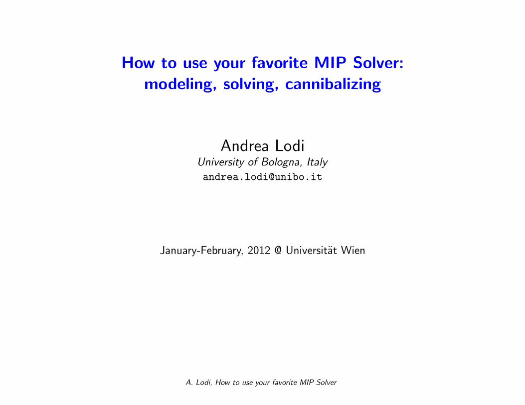
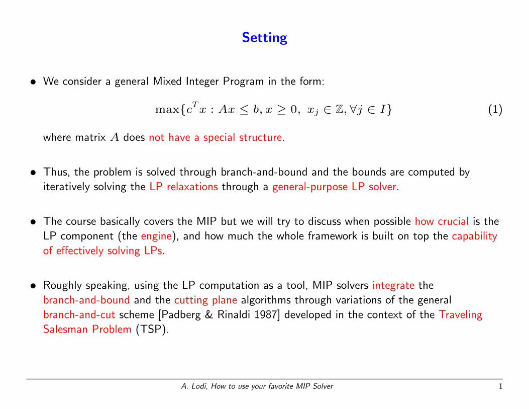
• We consider a general Mixed Integer Program in the form:
max{cTx : Ax ≤ b, x ≥ 0, xj ∈ Z, ∀j ∈ I} (1)
where matrix A does not have a special structure.
A. Lodi, How to use your favorite MIP Solver 1
Setting
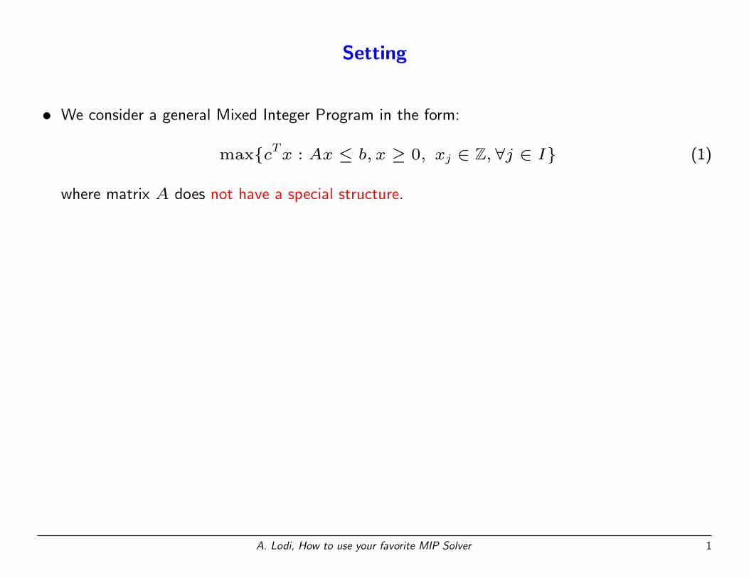
• We consider a general Mixed Integer Program in the form:
max{cTx : Ax ≤ b, x ≥ 0, xj ∈ Z, ∀j ∈ I} (1)
where matrix A does not have a special structure.
• Thus, the problem is solved through branch-and-bound and the bounds are computed by
iteratively solving the LP relaxations through a general-purpose LP solver.
A. Lodi, How to use your favorite MIP Solver 1
Setting
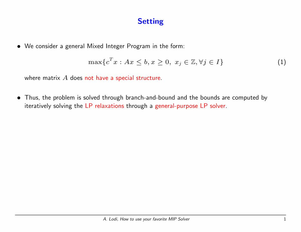
• We consider a general Mixed Integer Program in the form:
max{cTx : Ax ≤ b, x ≥ 0, xj ∈ Z, ∀j ∈ I} (1)
where matrix A does not have a special structure.
• Thus, the problem is solved through branch-and-bound and the bounds are computed by
iteratively solving the LP relaxations through a general-purpose LP solver.
• The course basically covers the MIP but we will try to discuss when possible how crucial is the
LP component (the engine), and how much the whole framework is built on top the capability
of effectively solving LPs.
• Roughly speaking, using the LP computation as a tool, MIP solvers integrate the
branch-and-bound and the cutting plane algorithms through variations of the general
branch-and-cut scheme [Padberg & Rinaldi 1987] developed in the context of the Traveling
Salesman Problem (TSP).
A. Lodi, How to use your favorite MIP Solver 1
Motivation
• I have been asked for a PhD course under the general title of Advanced Methods in
Optimization.
• So, a sensible question is
Why Mixed Integer Programming and especially MIP Solvers?
A. Lodi, How to use your favorite MIP Solver 2

Motivation
• I have been asked for a PhD course under the general title of Advanced Methods in
Optimization.
• So, a sensible question is
Why Mixed Integer Programming and especially MIP Solvers?
• An easy answer is that developing MIP methodology (and solvers) is what I have been doing for
the last 15 years. . .
A. Lodi, How to use your favorite MIP Solver 2
Motivation
• I have been asked for a PhD course under the general title of Advanced Methods in
Optimization.
• So, a sensible question is
Why Mixed Integer Programming and especially MIP Solvers?
• An easy answer is that developing MIP methodology (and solvers) is what I have been doing for
the last 15 years. . .
• However, one main point of talking about MIP and MIP solvers, and especially doing that in
Vienna, is that in the recent years MIP solvers have become effective, reliable and flexible tools
for algorithmic development and real-world solving.
• In other words, MIP technology as moved from theory to practice and the course will try to
establish the confidence and give the pointers to fully take advantage of MIP (solvers).
A. Lodi, How to use your favorite MIP Solver 2
Outline
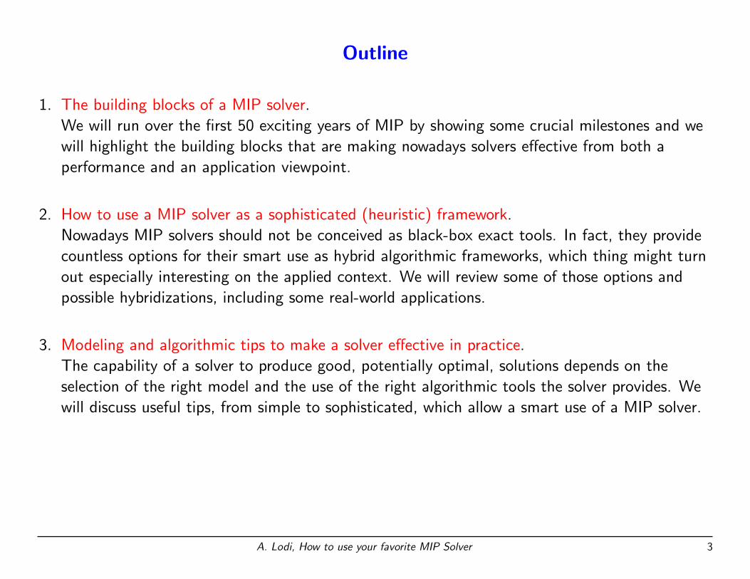
1. The building blocks of a MIP solver.
We will run over the first 50 exciting years of MIP by showing some crucial milestones and we
will highlight the building blocks that are making nowadays solvers effective from both a
performance and an application viewpoint.
A. Lodi, How to use your favorite MIP Solver 3
Outline
1. The building blocks of a MIP solver.
We will run over the first 50 exciting years of MIP by showing some crucial milestones and we
will highlight the building blocks that are making nowadays solvers effective from both a
performance and an application viewpoint.
2. How to use a MIP solver as a sophisticated (heuristic) framework.
Nowadays MIP solvers should not be conceived as black-box exact tools. In fact, they provide
countless options for their smart use as hybrid algorithmic frameworks, which thing might turn
out especially interesting on the applied context. We will review some of those options and
possible hybridizations, including some real-world applications.
3. Modeling and algorithmic tips to make a solver effective in practice.
The capability of a solver to produce good, potentially optimal, solutions depends on the
selection of the right model and the use of the right algorithmic tools the solver provides. We
will discuss useful tips, from simple to sophisticated, which allow a smart use of a MIP solver.
A. Lodi, How to use your favorite MIP Solver 3

Outline
1. The building blocks of a MIP solver.
We will run over the first 50 exciting years of MIP by showing some crucial milestones and we
will highlight the building blocks that are making nowadays solvers effective from both a
performance and an application viewpoint.
2. How to use a MIP solver as a sophisticated (heuristic) framework.
Nowadays MIP solvers should not be conceived as black-box exact tools. In fact, they provide
countless options for their smart use as hybrid algorithmic frameworks, which thing might turn
out especially interesting on the applied context. We will review some of those options and
possible hybridizations, including some real-world applications.
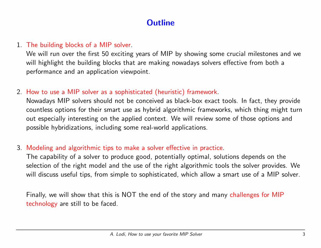
3. Modeling and algorithmic tips to make a solver effective in practice.
The capability of a solver to produce good, potentially optimal, solutions depends on the
selection of the right model and the use of the right algorithmic tools the solver provides. We
will discuss useful tips, from simple to sophisticated, which allow a smart use of a MIP solver.
Finally, we will show that this is NOT the end of the story and many challenges for MIP
technology are still to be faced.
A. Lodi, How to use your favorite MIP Solver 3
Outline
1. The building blocks of a MIP solver.
We will run over the first 50 exciting years of MIP by showing some crucial milestones and we
will highlight the building blocks that are making nowadays solvers effective from both a
performance and an application viewpoint.
2. How to use a MIP solver as a sophisticated (heuristic) framework.
Nowadays MIP solvers should not be conceived as black-box exact tools. In fact, they provide
countless options for their smart use as hybrid algorithmic frameworks, which thing might turn
out especially interesting on the applied context. We will review some of those options and
possible hybridizations, including some real-world applications.
3. Modeling and algorithmic tips to make a solver effective in practice.
The capability of a solver to produce good, potentially optimal, solutions depends on the
selection of the right model and the use of the right algorithmic tools the solver provides. We
will discuss useful tips, from simple to sophisticated, which allow a smart use of a MIP solver.
Finally, we will show that this is NOT the end of the story and many challenges for MIP
technology are still to be faced.
A. Lodi, How to use your favorite MIP Solver 3
PART 1
1. The building blocks of a MIP solver
2. How to use a MIP solver as a sophisticated (heuristic) framework
A. Lodi, How to use your favorite MIP Solver 4
PART 1
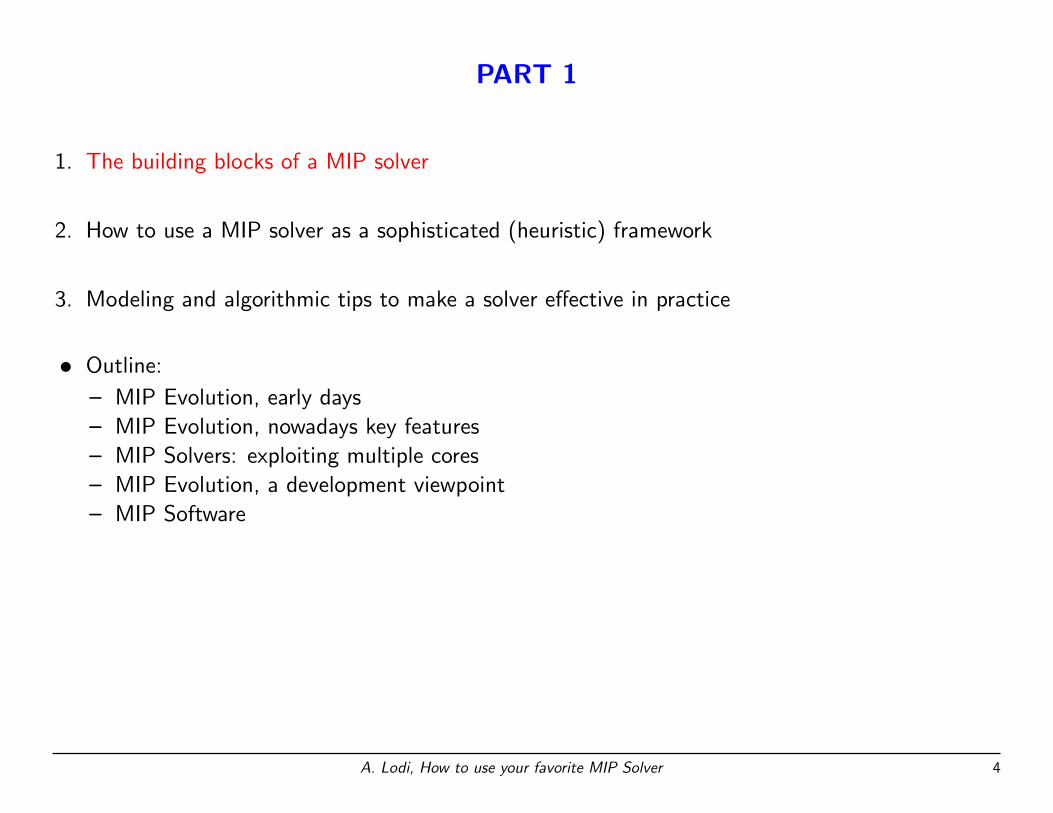
1. The building blocks of a MIP solver
2. How to use a MIP solver as a sophisticated (heuristic) framework
3. Modeling and algorithmic tips to make a solver effective in practice
• Outline:
– MIP Evolution, early days
– MIP Evolution, nowadays key features
– MIP Solvers: exploiting multiple cores
– MIP Evolution, a development viewpoint
– MIP Software
A. Lodi, How to use your favorite MIP Solver 4
MIP Evolution, early days
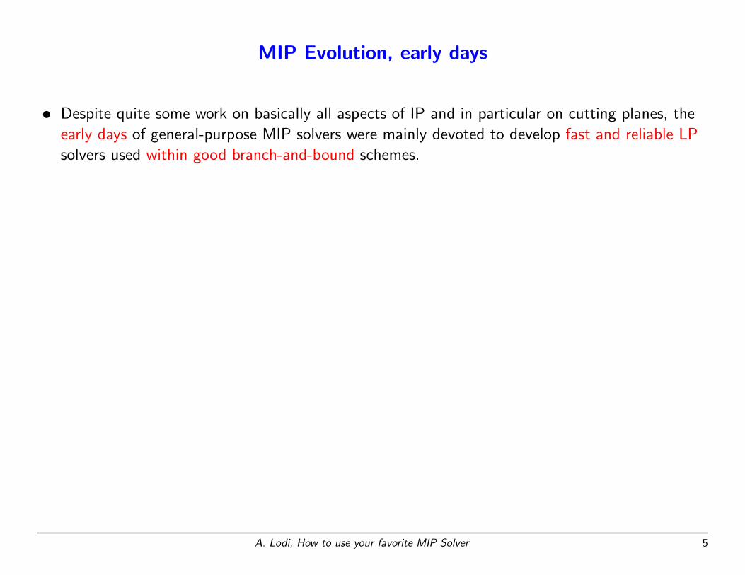
• Despite quite some work on basically all aspects of IP and in particular on cutting planes, the
early days of general-purpose MIP solvers were mainly devoted to develop fast and reliable LP
solvers used within good branch-and-bound schemes.
A. Lodi, How to use your favorite MIP Solver 5
MIP Evolution, early days
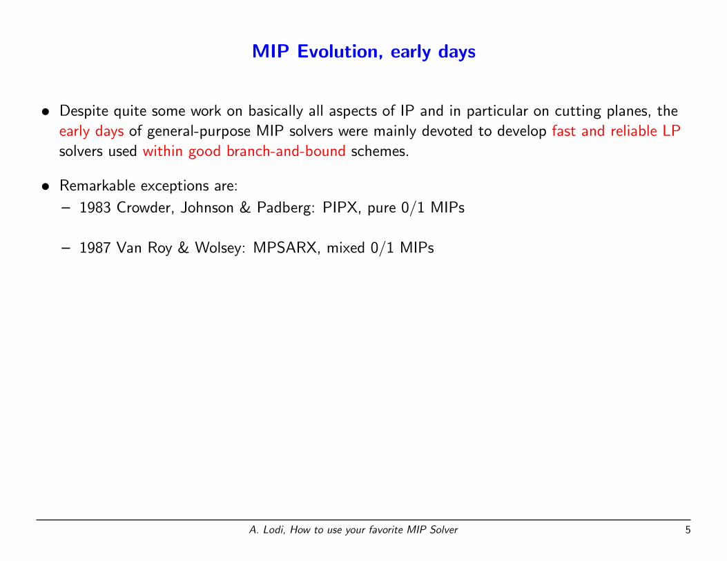
• Despite quite some work on basically all aspects of IP and in particular on cutting planes, the
early days of general-purpose MIP solvers were mainly devoted to develop fast and reliable LP
solvers used within good branch-and-bound schemes.
• Remarkable exceptions are:
– 1983 Crowder, Johnson & Padberg: PIPX, pure 0/1 MIPs
– 1987 Van Roy & Wolsey: MPSARX, mixed 0/1 MIPs
A. Lodi, How to use your favorite MIP Solver 5
MIP Evolution, early days
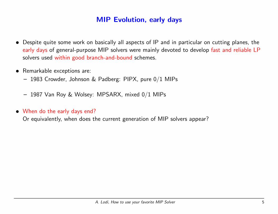
• Despite quite some work on basically all aspects of IP and in particular on cutting planes, the
early days of general-purpose MIP solvers were mainly devoted to develop fast and reliable LP
solvers used within good branch-and-bound schemes.
• Remarkable exceptions are:
– 1983 Crowder, Johnson & Padberg: PIPX, pure 0/1 MIPs
– 1987 Van Roy & Wolsey: MPSARX, mixed 0/1 MIPs
• When do the early days end?
Or equivalently, when does the current generation of MIP solvers appear?
A. Lodi, How to use your favorite MIP Solver 5
MIP Evolution, early days
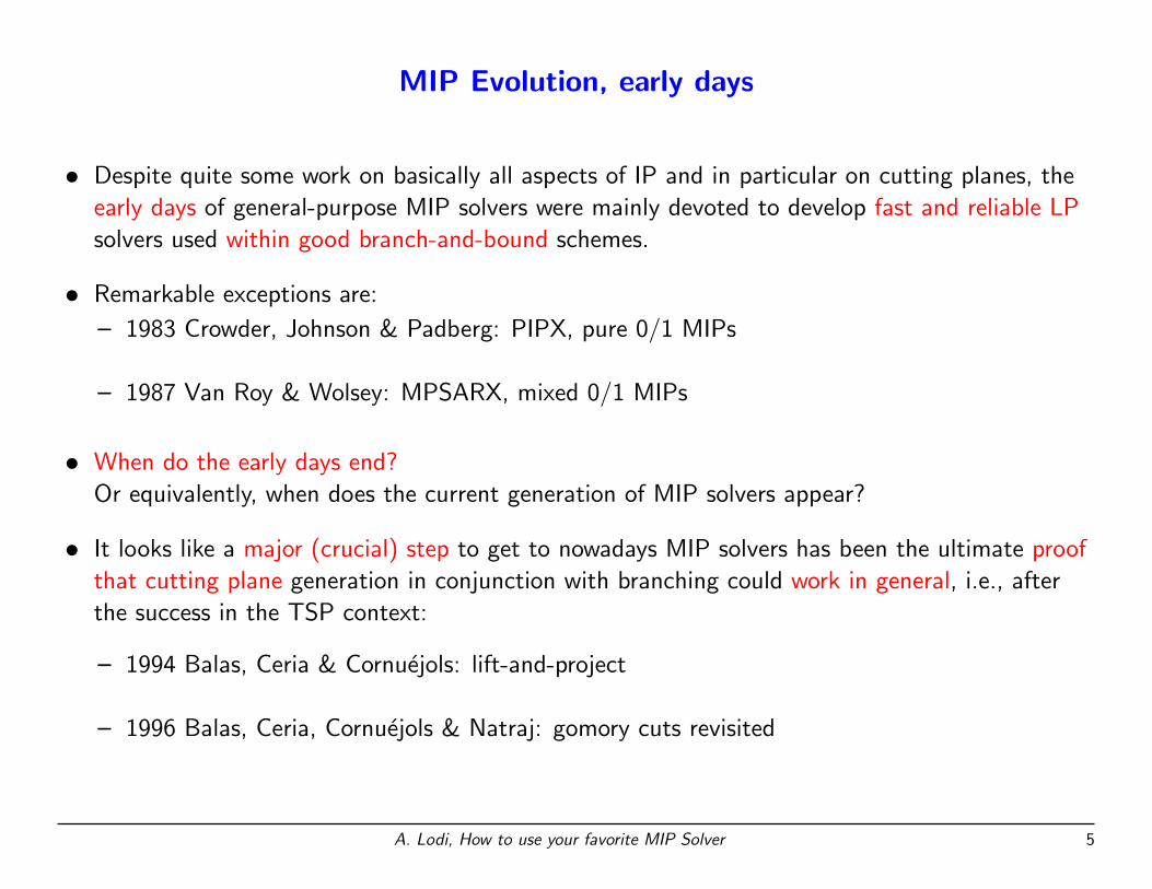
• Despite quite some work on basically all aspects of IP and in particular on cutting planes, the
early days of general-purpose MIP solvers were mainly devoted to develop fast and reliable LP
solvers used within good branch-and-bound schemes.
• Remarkable exceptions are:
– 1983 Crowder, Johnson & Padberg: PIPX, pure 0/1 MIPs
– 1987 Van Roy & Wolsey: MPSARX, mixed 0/1 MIPs
• When do the early days end?
Or equivalently, when does the current generation of MIP solvers appear?
• It looks like a major (crucial) step to get to nowadays MIP solvers has been the ultimate proof
that cutting plane generation in conjunction with branching could work in general, i.e., after
the success in the TSP context:
– 1994 Balas, Ceria & Cornuejols: lift-and-project
– 1996 Balas, Ceria, Cornuejols & Natraj: gomory cuts revisited
A. Lodi, How to use your favorite MIP Solver 5
MIP Evolution, Cplex numbers
• Bob Bixby (Gurobi) & Tobias Achterberg (IBM) performed the following interesting experiment
comparing Cplex versions from Cplex 1.2 (the first one with MIP capability) up to Cplex 11.0.
A. Lodi, How to use your favorite MIP Solver 6
MIP Evolution, Cplex numbers
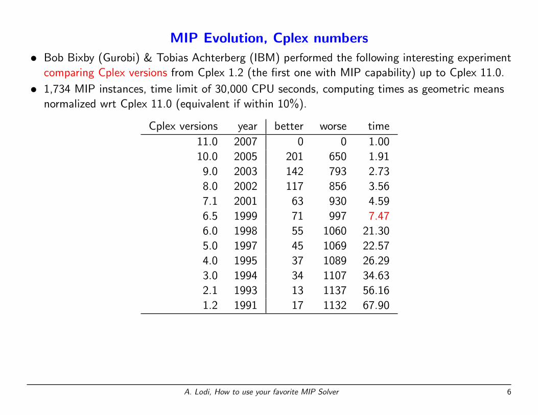
• Bob Bixby (Gurobi) & Tobias Achterberg (IBM) performed the following interesting experiment
comparing Cplex versions from Cplex 1.2 (the first one with MIP capability) up to Cplex 11.0.
• 1,734 MIP instances, time limit of 30,000 CPU seconds, computing times as geometric means
normalized wrt Cplex 11.0 (equivalent if within 10%).
Cplex versions year better worse time
11.0 2007 0 0 1.00
10.0 2005 201 650 1.91
9.0 2003 142 793 2.73
8.0 2002 117 856 3.56
7.1 2001 63 930 4.59
6.5 1999 71 997 7.47
6.0 1998 55 1060 21.30
5.0 1997 45 1069 22.57
4.0 1995 37 1089 26.29
3.0 1994 34 1107 34.63
2.1 1993 13 1137 56.16
1.2 1991 17 1132 67.90
A. Lodi, How to use your favorite MIP Solver 6
MIP Evolution, Cplex numbers
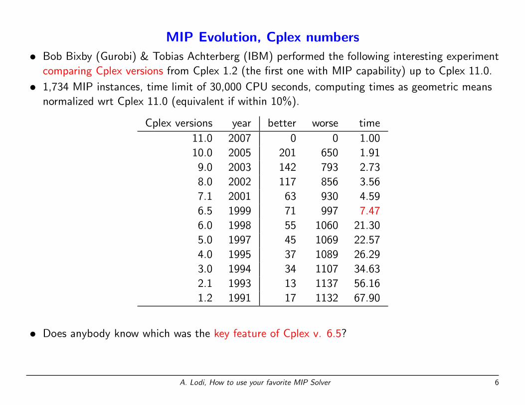
• Bob Bixby (Gurobi) & Tobias Achterberg (IBM) performed the following interesting experiment
comparing Cplex versions from Cplex 1.2 (the first one with MIP capability) up to Cplex 11.0.
• 1,734 MIP instances, time limit of 30,000 CPU seconds, computing times as geometric means
normalized wrt Cplex 11.0 (equivalent if within 10%).
Cplex versions year better worse time
11.0 2007 0 0 1.00
10.0 2005 201 650 1.91
9.0 2003 142 793 2.73
8.0 2002 117 856 3.56
7.1 2001 63 930 4.59
6.5 1999 71 997 7.47
6.0 1998 55 1060 21.30
5.0 1997 45 1069 22.57
4.0 1995 37 1089 26.29
3.0 1994 34 1107 34.63
2.1 1993 13 1137 56.16
1.2 1991 17 1132 67.90
• Does anybody know which was the key feature of Cplex v. 6.5?
A. Lodi, How to use your favorite MIP Solver 6
MIP Evolution, Cutting Planes
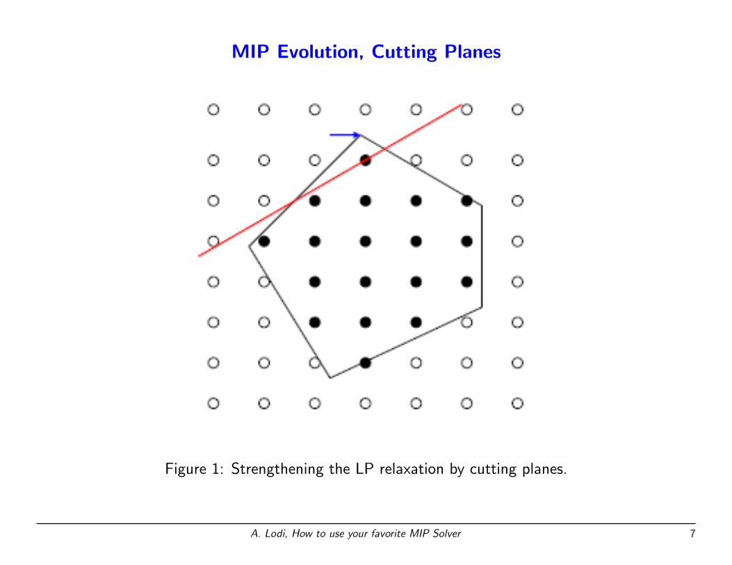
Figure 1: Strengthening the LP relaxation by cutting planes.
A. Lodi, How to use your favorite MIP Solver 7
MIP Evolution, nowadays key features
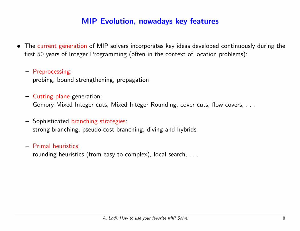
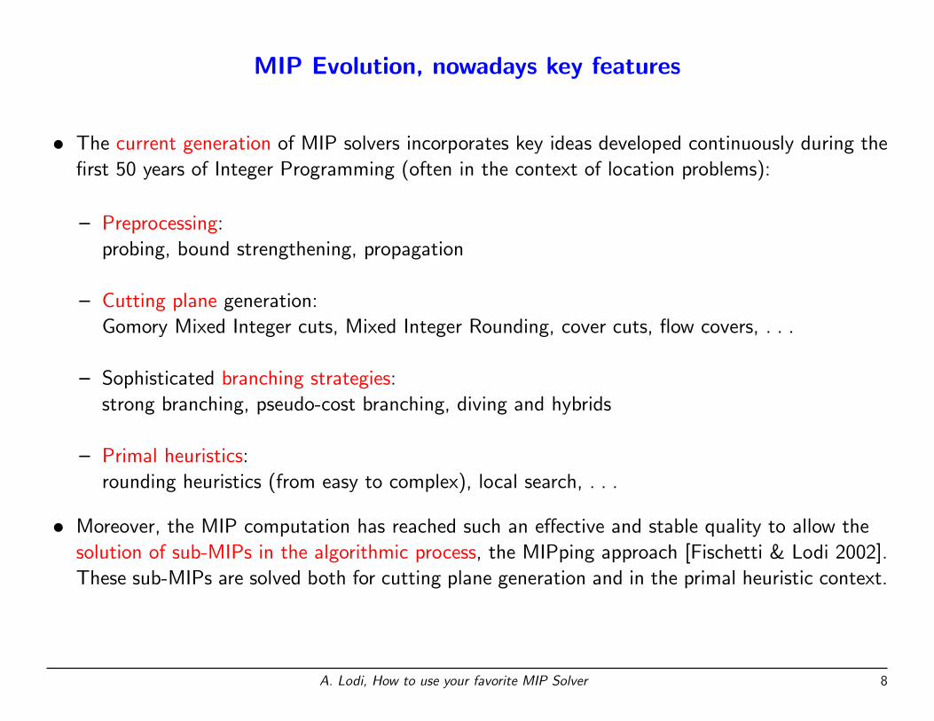
• The current generation of MIP solvers incorporates key ideas developed continuously during the
first 50 years of Integer Programming (often in the context of location problems):
A. Lodi, How to use your favorite MIP Solver 8
MIP Evolution, nowadays key features
• The current generation of MIP solvers incorporates key ideas developed continuously during the
first 50 years of Integer Programming (often in the context of location problems):
– Preprocessing:
probing, bound strengthening, propagation
– Cutting plane generation:
Gomory Mixed Integer cuts, Mixed Integer Rounding, cover cuts, flow covers, . . .
– Sophisticated branching strategies:
strong branching, pseudo-cost branching, diving and hybrids
– Primal heuristics:
rounding heuristics (from easy to complex), local search, . . .
• Moreover, the MIP computation has reached such an effective and stable quality to allow the
solution of sub-MIPs in the algorithmic process, the MIPping approach [Fischetti & Lodi 2002].
These sub-MIPs are solved both for cutting plane generation and in the primal heuristic context.
A. Lodi, How to use your favorite MIP Solver 8
MIP Building Blocks: Preprocessing/Presolving
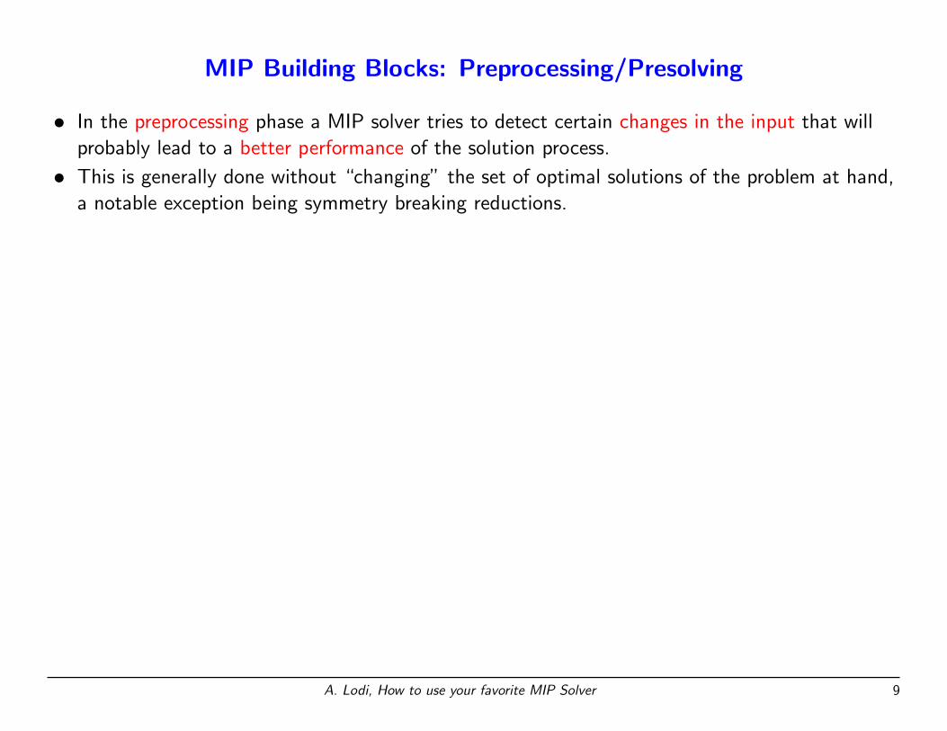
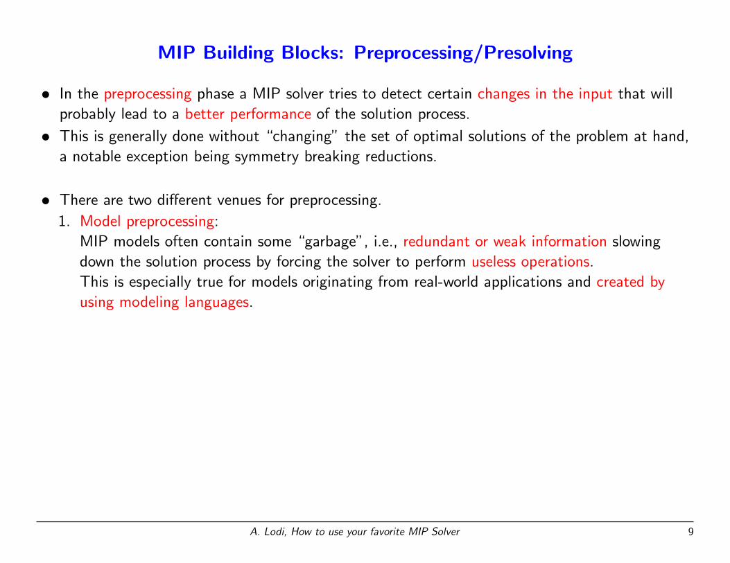
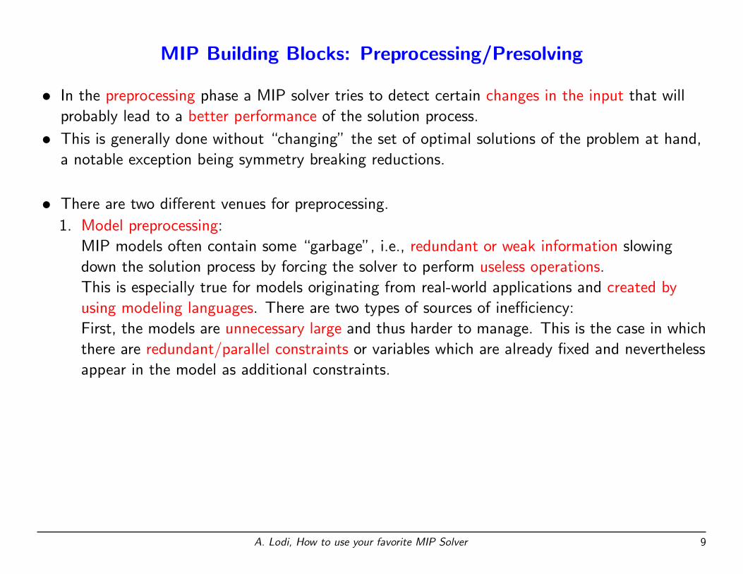
• In the preprocessing phase a MIP solver tries to detect certain changes in the input that will
probably lead to a better performance of the solution process.
• This is generally done without “changing” the set of optimal solutions of the problem at hand,
a notable exception being symmetry breaking reductions.
A. Lodi, How to use your favorite MIP Solver 9
MIP Building Blocks: Preprocessing/Presolving
• In the preprocessing phase a MIP solver tries to detect certain changes in the input that will
probably lead to a better performance of the solution process.
• This is generally done without “changing” the set of optimal solutions of the problem at hand,
a notable exception being symmetry breaking reductions.
• There are two different venues for preprocessing.
1. Model preprocessing:
MIP models often contain some “garbage”, i.e., redundant or weak information slowing
down the solution process by forcing the solver to perform useless operations.
This is especially true for models originating from real-world applications and created by
using modeling languages.
A. Lodi, How to use your favorite MIP Solver 9
MIP Building Blocks: Preprocessing/Presolving
• In the preprocessing phase a MIP solver tries to detect certain changes in the input that will
probably lead to a better performance of the solution process.
• This is generally done without “changing” the set of optimal solutions of the problem at hand,
a notable exception being symmetry breaking reductions.
• There are two different venues for preprocessing.
1. Model preprocessing:
MIP models often contain some “garbage”, i.e., redundant or weak information slowing
down the solution process by forcing the solver to perform useless operations.
This is especially true for models originating from real-world applications and created by
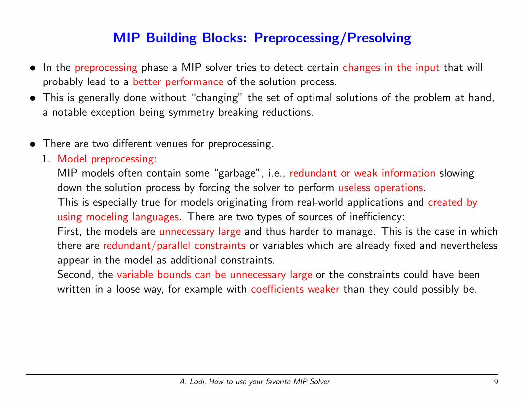
using modeling languages. There are two types of sources of inefficiency:
First, the models are unnecessary large and thus harder to manage. This is the case in which
there are redundant/parallel constraints or variables which are already fixed and nevertheless
appear in the model as additional constraints.
A. Lodi, How to use your favorite MIP Solver 9
MIP Building Blocks: Preprocessing/Presolving
• In the preprocessing phase a MIP solver tries to detect certain changes in the input that will
probably lead to a better performance of the solution process.
• This is generally done without “changing” the set of optimal solutions of the problem at hand,
a notable exception being symmetry breaking reductions.
• There are two different venues for preprocessing.
1. Model preprocessing:
MIP models often contain some “garbage”, i.e., redundant or weak information slowing
down the solution process by forcing the solver to perform useless operations.
This is especially true for models originating from real-world applications and created by
using modeling languages. There are two types of sources of inefficiency:
First, the models are unnecessary large and thus harder to manage. This is the case in which
there are redundant/parallel constraints or variables which are already fixed and nevertheless
appear in the model as additional constraints.
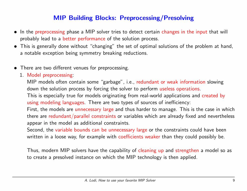
Second, the variable bounds can be unnecessary large or the constraints could have been
written in a loose way, for example with coefficients weaker than they could possibly be.
A. Lodi, How to use your favorite MIP Solver 9
MIP Building Blocks: Preprocessing/Presolving
• In the preprocessing phase a MIP solver tries to detect certain changes in the input that will
probably lead to a better performance of the solution process.
• This is generally done without “changing” the set of optimal solutions of the problem at hand,
a notable exception being symmetry breaking reductions.
• There are two different venues for preprocessing.
1. Model preprocessing:
MIP models often contain some “garbage”, i.e., redundant or weak information slowing
down the solution process by forcing the solver to perform useless operations.
This is especially true for models originating from real-world applications and created by
using modeling languages. There are two types of sources of inefficiency:
First, the models are unnecessary large and thus harder to manage. This is the case in which
there are redundant/parallel constraints or variables which are already fixed and nevertheless
appear in the model as additional constraints.
Second, the variable bounds can be unnecessary large or the constraints could have been
written in a loose way, for example with coefficients weaker than they could possibly be.
Thus, modern MIP solvers have the capability of cleaning up and strengthen a model so as
to create a presolved instance on which the MIP technology is then applied.
A. Lodi, How to use your favorite MIP Solver 9
MIP Building Blocks: Preprocessing/Presolving (cont.d)
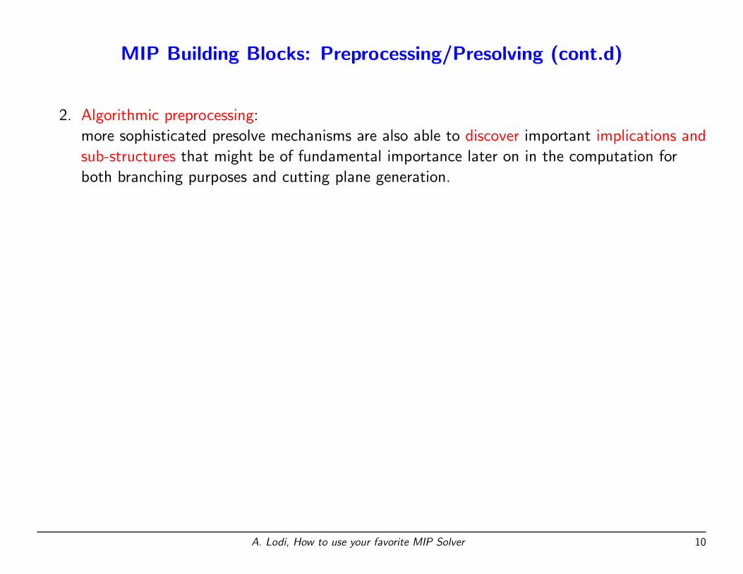
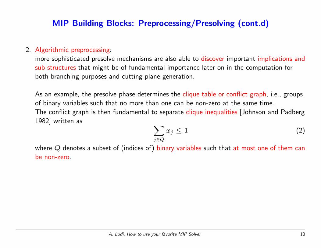
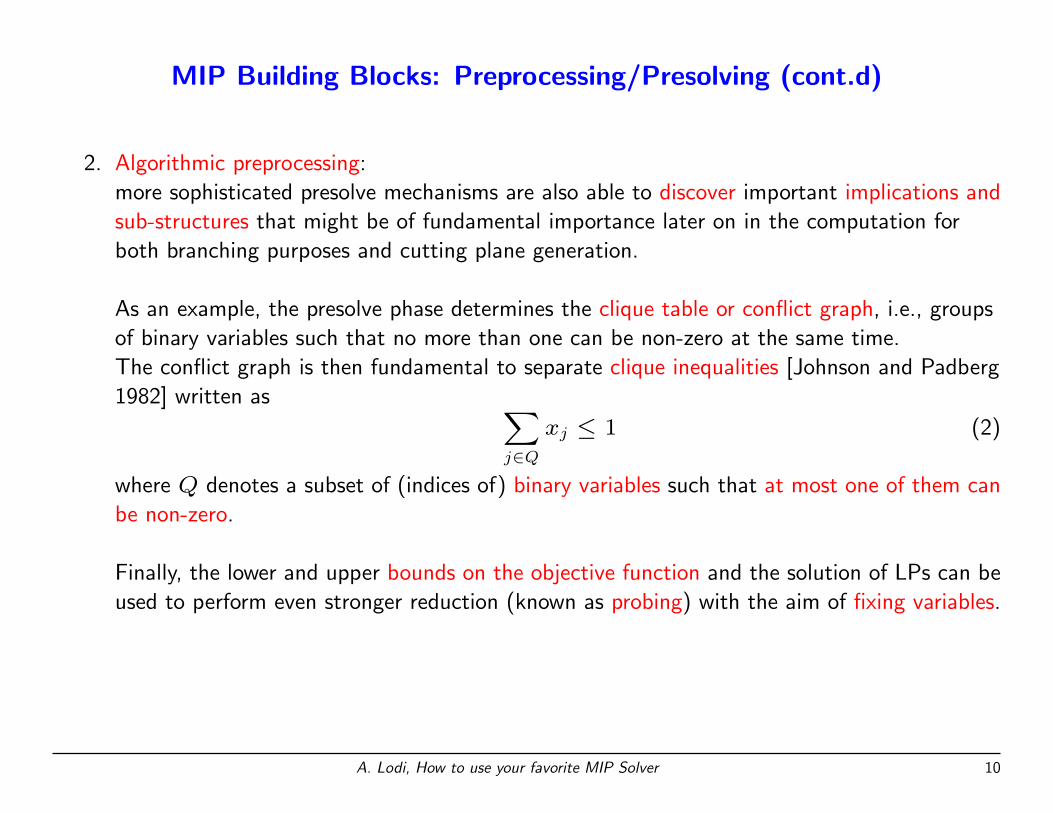
2. Algorithmic preprocessing:
more sophisticated presolve mechanisms are also able to discover important implications and
sub-structures that might be of fundamental importance later on in the computation for
both branching purposes and cutting plane generation.
A. Lodi, How to use your favorite MIP Solver 10
MIP Building Blocks: Preprocessing/Presolving (cont.d)
2. Algorithmic preprocessing:
more sophisticated presolve mechanisms are also able to discover important implications and
sub-structures that might be of fundamental importance later on in the computation for
both branching purposes and cutting plane generation.
As an example, the presolve phase determines the clique table or conflict graph, i.e., groups
of binary variables such that no more than one can be non-zero at the same time.
The conflict graph is then fundamental to separate clique inequalities [Johnson and Padberg
1982] written as ∑j∈Q
xj ≤ 1 (2)
where Q denotes a subset of (indices of) binary variables such that at most one of them can
be non-zero.
Finally, the lower and upper bounds on the objective function and the solution of LPs can be
used to perform even stronger reduction (known as probing) with the aim of fixing variables.
A. Lodi, How to use your favorite MIP Solver 10
MIP Building Blocks: Cutting Planes
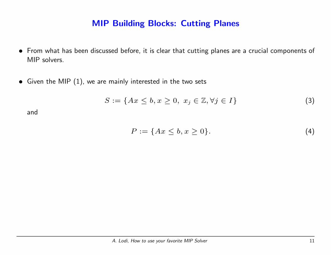
• From what has been discussed before, it is clear that cutting planes are a crucial components of
MIP solvers.
A. Lodi, How to use your favorite MIP Solver 11
MIP Building Blocks: Cutting Planes
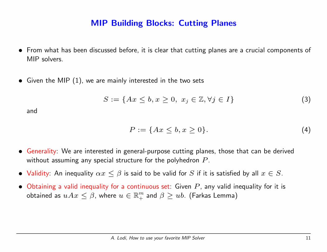
• From what has been discussed before, it is clear that cutting planes are a crucial components of
MIP solvers.
• Given the MIP (1), we are mainly interested in the two sets
S := {Ax ≤ b, x ≥ 0, xj ∈ Z, ∀j ∈ I} (3)
and
P := {Ax ≤ b, x ≥ 0}. (4)
A. Lodi, How to use your favorite MIP Solver 11
MIP Building Blocks: Cutting Planes
• From what has been discussed before, it is clear that cutting planes are a crucial components of
MIP solvers.
• Given the MIP (1), we are mainly interested in the two sets
S := {Ax ≤ b, x ≥ 0, xj ∈ Z, ∀j ∈ I} (3)
and
P := {Ax ≤ b, x ≥ 0}. (4)
• Generality: We are interested in general-purpose cutting planes, those that can be derived
without assuming any special structure for the polyhedron P .
• Validity: An inequality αx ≤ β is said to be valid for S if it is satisfied by all x ∈ S.
• Obtaining a valid inequality for a continuous set: Given P , any valid inequality for it is
obtained as uAx ≤ β, where u ∈ Rm+ and β ≥ ub. (Farkas Lemma)
A. Lodi, How to use your favorite MIP Solver 11
MIP Building Blocks: Cutting Planes (cont.d)
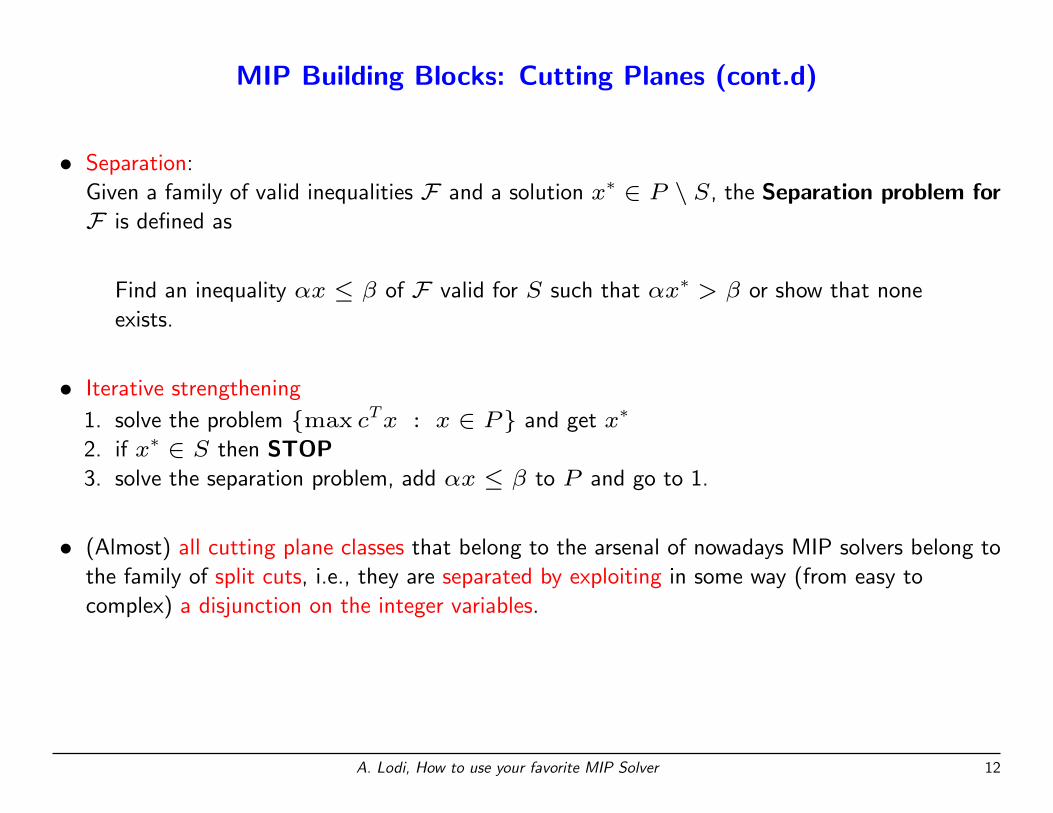
• Separation:
Given a family of valid inequalities F and a solution x∗ ∈ P \ S, the Separation problem forF is defined as
Find an inequality αx ≤ β of F valid for S such that αx∗ > β or show that none
exists.
• Iterative strengthening
1. solve the problem {max cTx : x ∈ P} and get x∗
2. if x∗ ∈ S then STOP3. solve the separation problem, add αx ≤ β to P and go to 1.
• (Almost) all cutting plane classes that belong to the arsenal of nowadays MIP solvers belong to
the family of split cuts, i.e., they are separated by exploiting in some way (from easy to
complex) a disjunction on the integer variables.
A. Lodi, How to use your favorite MIP Solver 12
MIP Building Blocks: Cutting Planes (cont.d)
• A basic rounding argument:
If x ∈ Z and x ≤ f f 6∈ Z, then x ≤ bfc.
A. Lodi, How to use your favorite MIP Solver 13
MIP Building Blocks: Cutting Planes (cont.d)
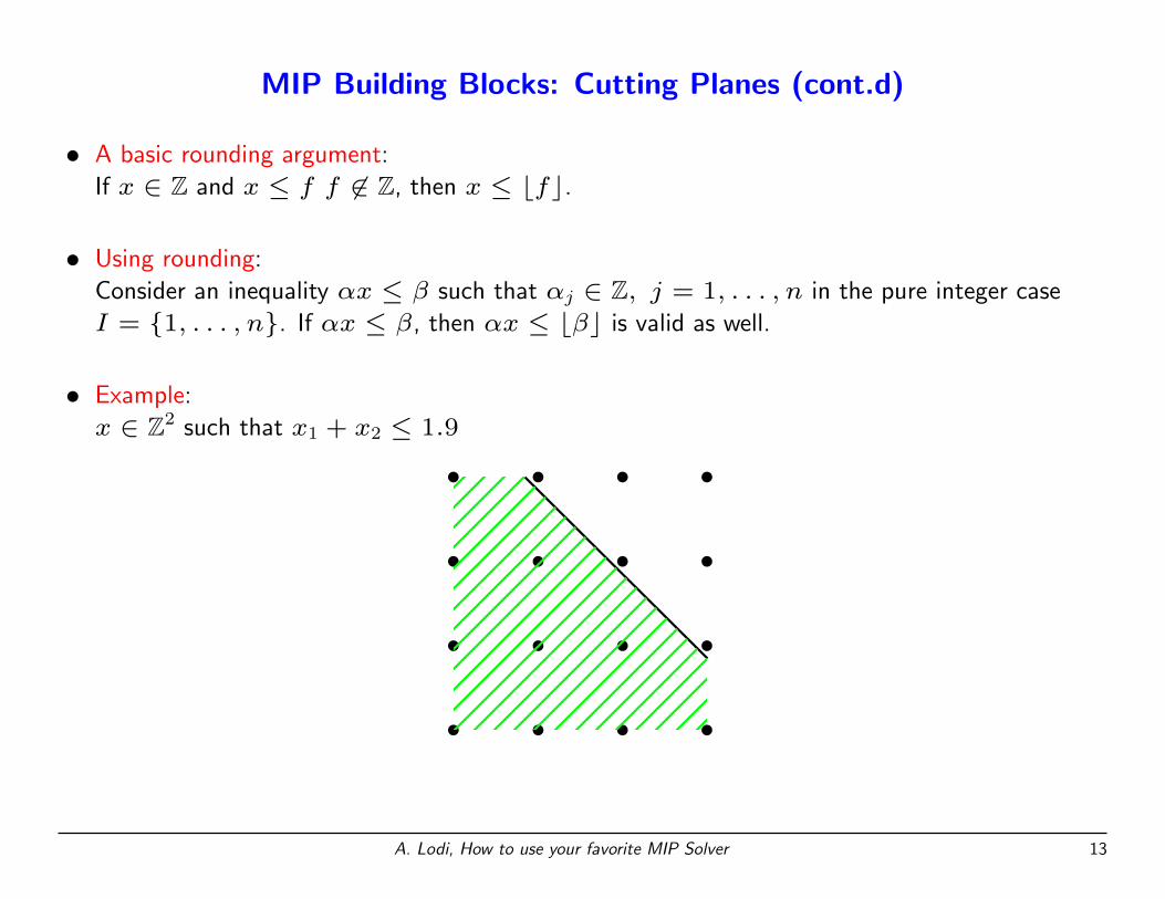
• A basic rounding argument:
If x ∈ Z and x ≤ f f 6∈ Z, then x ≤ bfc.
• Using rounding:
Consider an inequality αx ≤ β such that αj ∈ Z, j = 1, . . . , n in the pure integer case
I = {1, . . . , n}. If αx ≤ β, then αx ≤ bβc is valid as well.
A. Lodi, How to use your favorite MIP Solver 13
MIP Building Blocks: Cutting Planes (cont.d)
• A basic rounding argument:
If x ∈ Z and x ≤ f f 6∈ Z, then x ≤ bfc.
• Using rounding:
Consider an inequality αx ≤ β such that αj ∈ Z, j = 1, . . . , n in the pure integer case
I = {1, . . . , n}. If αx ≤ β, then αx ≤ bβc is valid as well.
• Example:
x ∈ Z2 such that x1 + x2 ≤ 1.9
2. Basic rounding
A basic rounding argument
If x ! Z and x " f f #! Z, then x " $f %.Using rounding
Consider an inequality !x " " such that !j ! Z, j = 1, . . . , n inthe pure integer case I = {1, . . . , n}. If !x " ", then !x " $"% isvalid as well.
Example
x ! Z2 such that x1 + x2 " 1.9
A. Lodi, How to use your favorite MIP Solver 13
MIP Building Blocks: Cutting Planes (cont.d)
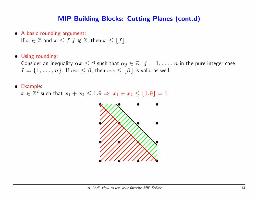
• A basic rounding argument:
If x ∈ Z and x ≤ f f 6∈ Z, then x ≤ bfc.
• Using rounding:
Consider an inequality αx ≤ β such that αj ∈ Z, j = 1, . . . , n in the pure integer case
I = {1, . . . , n}. If αx ≤ β, then αx ≤ bβc is valid as well.
• Example:
x ∈ Z2 such that x1 + x2 ≤ 1.9⇒ x1 + x2 ≤ b1.9c = 1
2. Basic rounding
A basic rounding argument
If x ! Z and x " f f #! Z, then x " $f %.Using rounding
Consider an inequality !x " " such that !j ! Z, j = 1, . . . , n inthe pure integer case I = {1, . . . , n}. If !x " ", then !x " $"% isvalid as well.
Example
x ! Z2 such that x1 + x2 " 1.9 & x1 + x2 " $1.9% = 1
A. Lodi, How to use your favorite MIP Solver 14
MIP Building Blocks: Cutting Planes (cont.d)
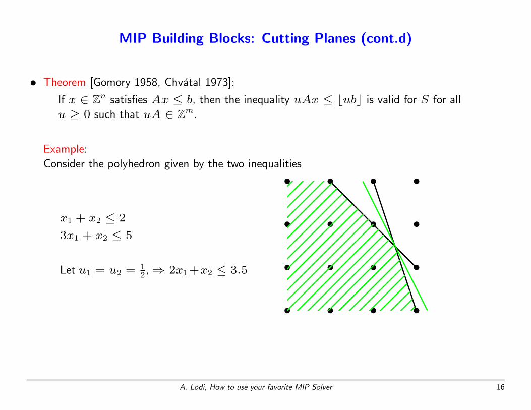
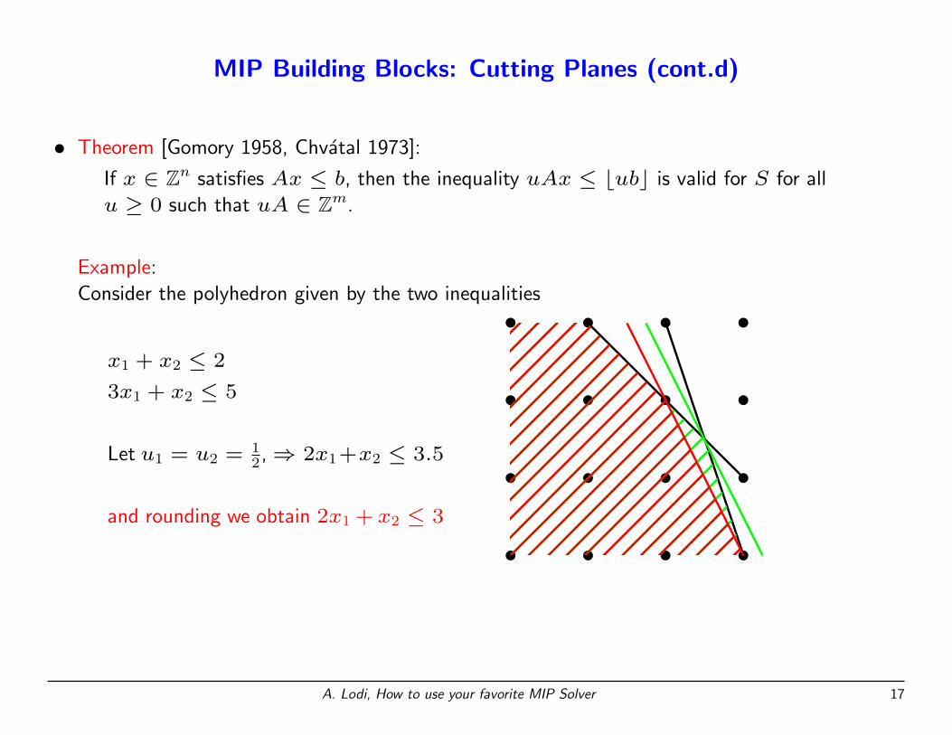
• Theorem [Gomory 1958, Chvatal 1973]:
If x ∈ Zn satisfies Ax ≤ b, then the inequality uAx ≤ bubc is valid for S for all
u ≥ 0 such that uA ∈ Zm.
A. Lodi, How to use your favorite MIP Solver 15
MIP Building Blocks: Cutting Planes (cont.d)
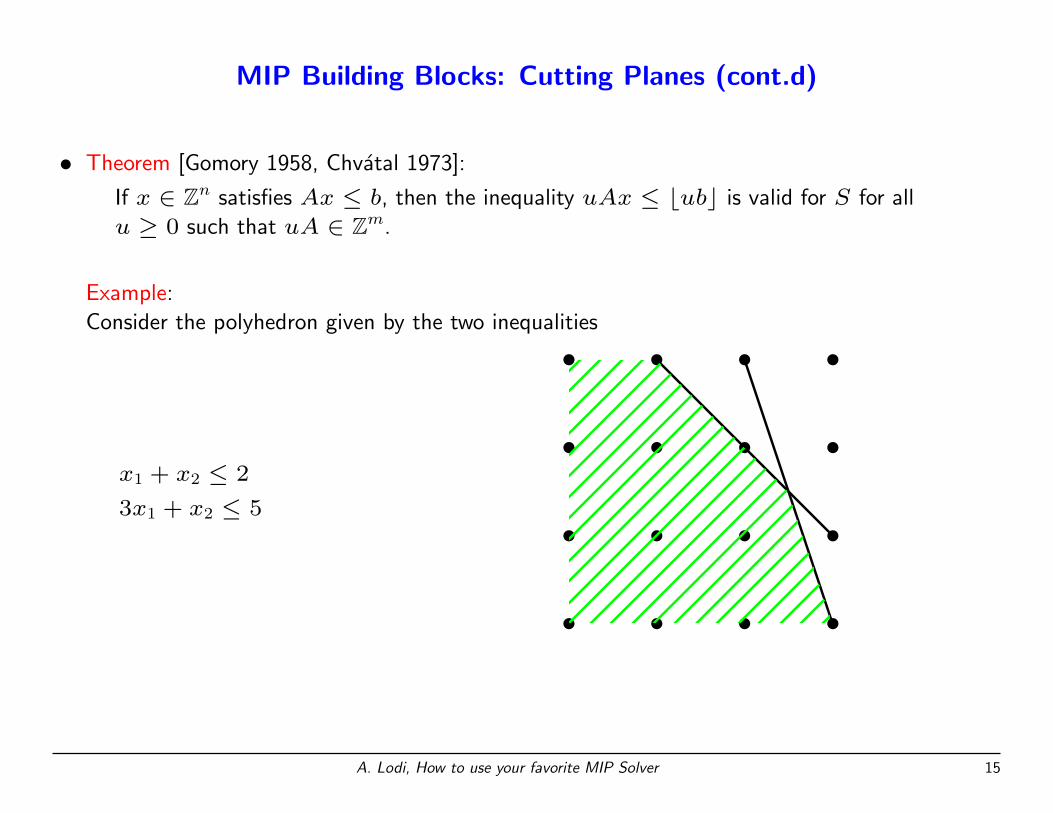
• Theorem [Gomory 1958, Chvatal 1973]:
If x ∈ Zn satisfies Ax ≤ b, then the inequality uAx ≤ bubc is valid for S for all
u ≥ 0 such that uA ∈ Zm.
Example:
Consider the polyhedron given by the two inequalities
x1 + x2 ≤ 2
3x1 + x2 ≤ 5
2. Chvatal-Gomory cuts, [Gomory 1958, Chvatal 1973]
TheoremIf x ! Zn satisfies Ax " b, then the inequality uAx " #ub$ is validfor S for all u % 0 such that uA ! Zm.
Example
Consider the polyhedron given by the two inequalities
x1 + x2 " 2
3x1 + x2 " 5
A. Lodi, How to use your favorite MIP Solver 15
MIP Building Blocks: Cutting Planes (cont.d)
• Theorem [Gomory 1958, Chvatal 1973]:
If x ∈ Zn satisfies Ax ≤ b, then the inequality uAx ≤ bubc is valid for S for all
u ≥ 0 such that uA ∈ Zm.
Example:
Consider the polyhedron given by the two inequalities
x1 + x2 ≤ 2
3x1 + x2 ≤ 5
Let u1 = u2 = 12,⇒ 2x1+x2 ≤ 3.5
2. Chvatal-Gomory cuts, [Gomory 1958, Chvatal 1973]
TheoremIf x ! Zn satisfies Ax " b, then the inequality uAx " #ub$ is validfor S for all u % 0 such that uA ! Zm.
Example
Consider the polyhedron given by the two inequalities
x1 + x2 " 2
3x1 + x2 " 5
Let u1 = u2 = 1/2, then
2x1 + x2 " 3.5
A. Lodi, How to use your favorite MIP Solver 16
MIP Building Blocks: Cutting Planes (cont.d)
• Theorem [Gomory 1958, Chvatal 1973]:
If x ∈ Zn satisfies Ax ≤ b, then the inequality uAx ≤ bubc is valid for S for all
u ≥ 0 such that uA ∈ Zm.
Example:
Consider the polyhedron given by the two inequalities
x1 + x2 ≤ 2
3x1 + x2 ≤ 5
Let u1 = u2 = 12,⇒ 2x1+x2 ≤ 3.5
and rounding we obtain 2x1 + x2 ≤ 3
2. Chvatal-Gomory cuts, [Gomory 1958, Chvatal 1973]
TheoremIf x ! Zn satisfies Ax " b, then the inequality uAx " #ub$ is validfor S for all u % 0 such that uA ! Zm.
Example
Consider the polyhedron given by the two inequalities
x1 + x2 " 2
3x1 + x2 " 5
Let u1 = u2 = 1/2, then
2x1 + x2 " 3.5
and rounding we obtain
2x1 + x2 " 3
A. Lodi, How to use your favorite MIP Solver 17
MIP Building Blocks: Branching
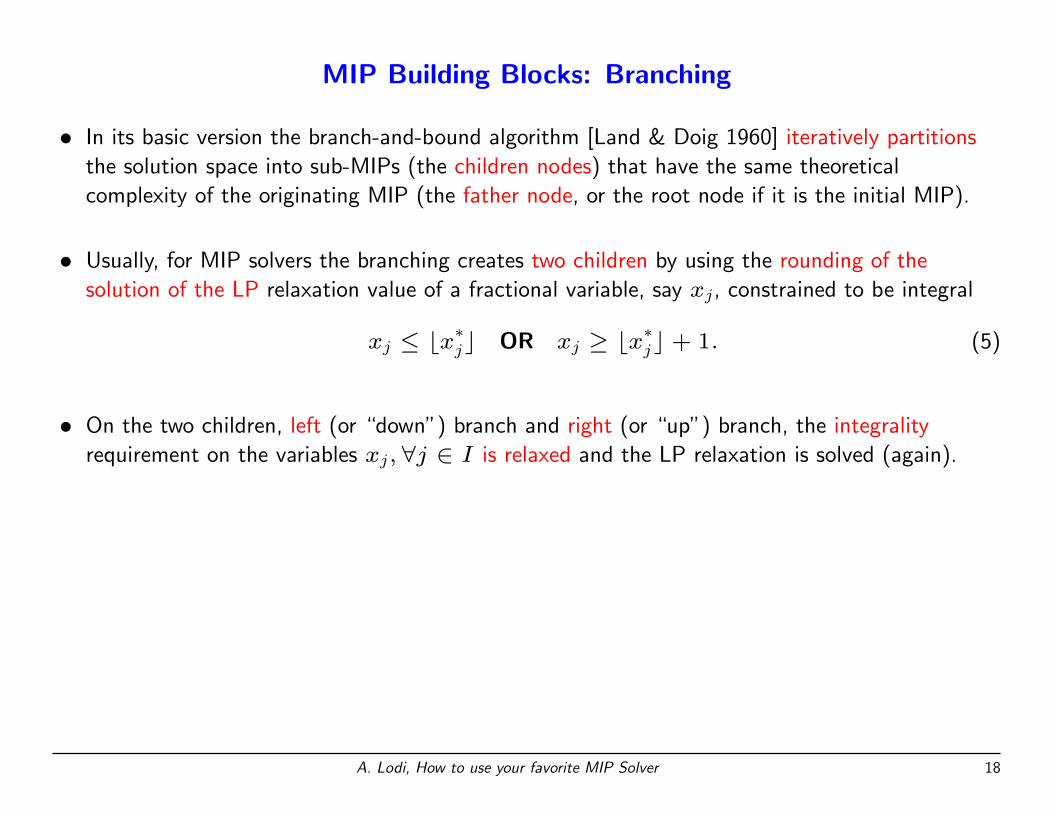
• In its basic version the branch-and-bound algorithm [Land & Doig 1960] iteratively partitions
the solution space into sub-MIPs (the children nodes) that have the same theoretical
complexity of the originating MIP (the father node, or the root node if it is the initial MIP).
A. Lodi, How to use your favorite MIP Solver 18
MIP Building Blocks: Branching
• In its basic version the branch-and-bound algorithm [Land & Doig 1960] iteratively partitions
the solution space into sub-MIPs (the children nodes) that have the same theoretical
complexity of the originating MIP (the father node, or the root node if it is the initial MIP).
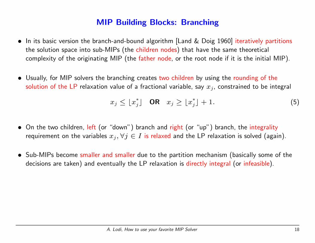
• Usually, for MIP solvers the branching creates two children by using the rounding of the
solution of the LP relaxation value of a fractional variable, say xj, constrained to be integral
xj ≤ bx∗jc OR xj ≥ bx∗jc+ 1. (5)
A. Lodi, How to use your favorite MIP Solver 18
MIP Building Blocks: Branching
• In its basic version the branch-and-bound algorithm [Land & Doig 1960] iteratively partitions
the solution space into sub-MIPs (the children nodes) that have the same theoretical
complexity of the originating MIP (the father node, or the root node if it is the initial MIP).
• Usually, for MIP solvers the branching creates two children by using the rounding of the
solution of the LP relaxation value of a fractional variable, say xj, constrained to be integral
xj ≤ bx∗jc OR xj ≥ bx∗jc+ 1. (5)
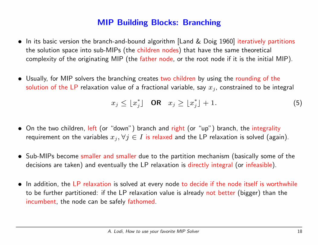
• On the two children, left (or “down”) branch and right (or “up”) branch, the integrality
requirement on the variables xj, ∀j ∈ I is relaxed and the LP relaxation is solved (again).
A. Lodi, How to use your favorite MIP Solver 18
MIP Building Blocks: Branching
• In its basic version the branch-and-bound algorithm [Land & Doig 1960] iteratively partitions
the solution space into sub-MIPs (the children nodes) that have the same theoretical
complexity of the originating MIP (the father node, or the root node if it is the initial MIP).
• Usually, for MIP solvers the branching creates two children by using the rounding of the
solution of the LP relaxation value of a fractional variable, say xj, constrained to be integral
xj ≤ bx∗jc OR xj ≥ bx∗jc+ 1. (5)
• On the two children, left (or “down”) branch and right (or “up”) branch, the integrality
requirement on the variables xj, ∀j ∈ I is relaxed and the LP relaxation is solved (again).
• Sub-MIPs become smaller and smaller due to the partition mechanism (basically some of the
decisions are taken) and eventually the LP relaxation is directly integral (or infeasible).
• In addition, the LP relaxation is solved at every node to decide if the node itself is worthwhile
to be further partitioned: if the LP relaxation value is already not better (bigger) than the
incumbent, the node can be safely fathomed.
A. Lodi, How to use your favorite MIP Solver 18
MIP Building Blocks: Branching (cont.d)
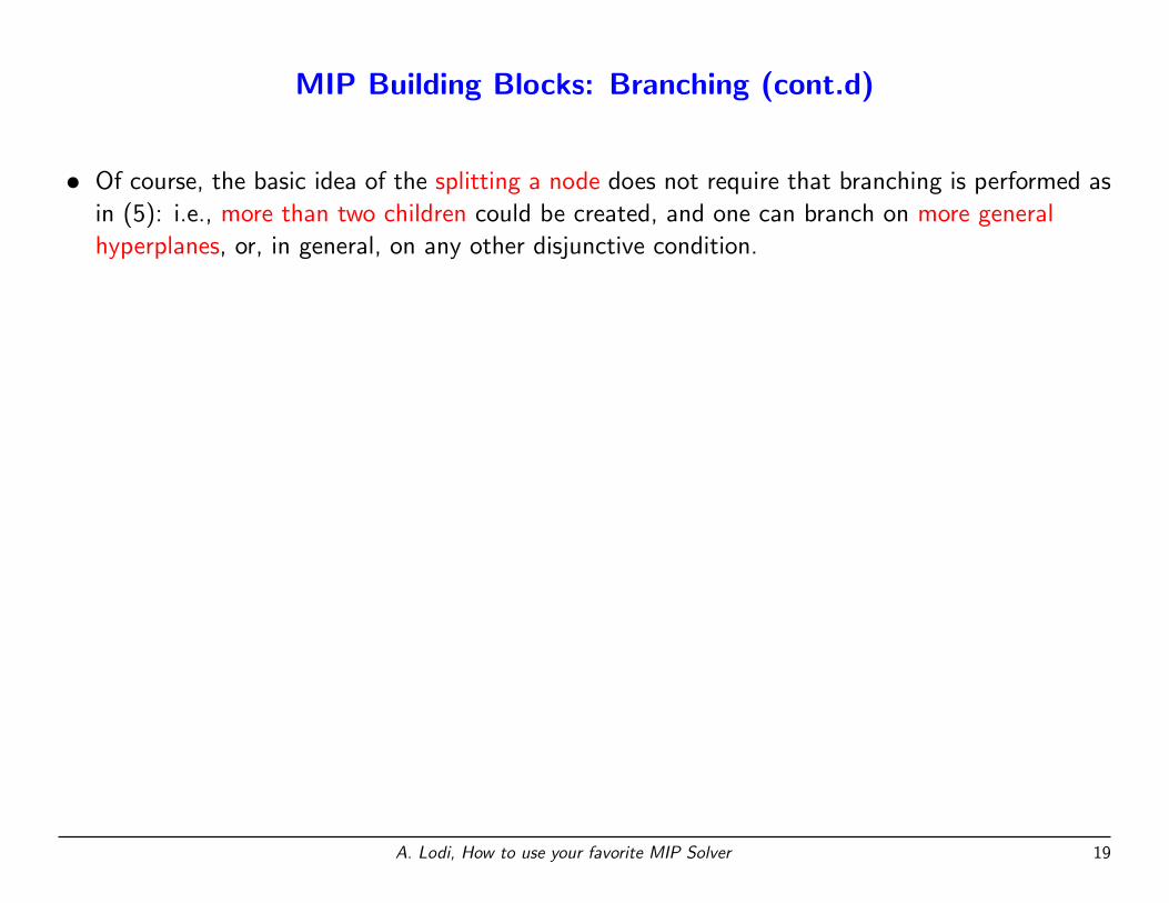
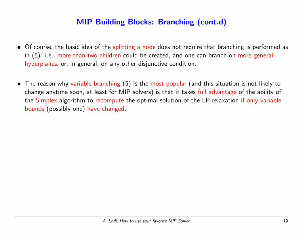
• Of course, the basic idea of the splitting a node does not require that branching is performed as
in (5): i.e., more than two children could be created, and one can branch on more general
hyperplanes, or, in general, on any other disjunctive condition.
A. Lodi, How to use your favorite MIP Solver 19
MIP Building Blocks: Branching (cont.d)
• Of course, the basic idea of the splitting a node does not require that branching is performed as
in (5): i.e., more than two children could be created, and one can branch on more general
hyperplanes, or, in general, on any other disjunctive condition.
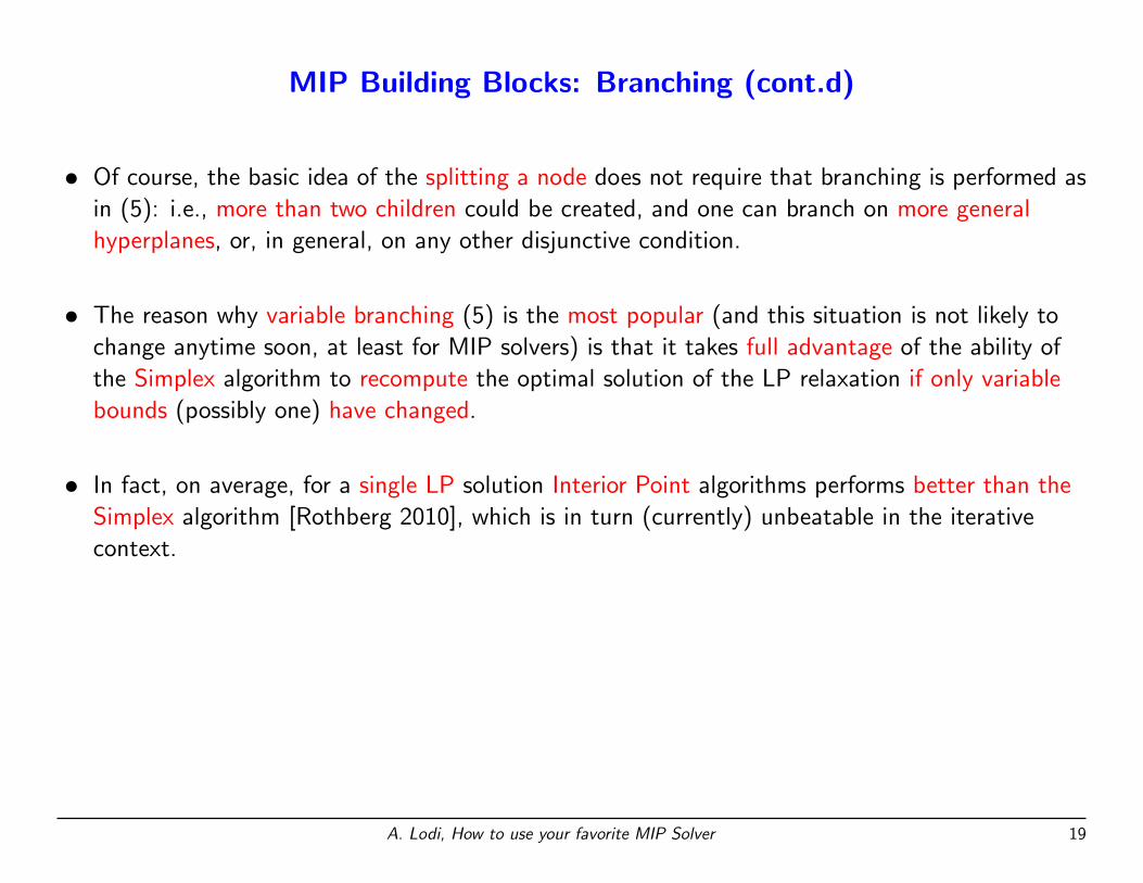
• The reason why variable branching (5) is the most popular (and this situation is not likely to
change anytime soon, at least for MIP solvers) is that it takes full advantage of the ability of
the Simplex algorithm to recompute the optimal solution of the LP relaxation if only variable
bounds (possibly one) have changed.
A. Lodi, How to use your favorite MIP Solver 19
MIP Building Blocks: Branching (cont.d)
• Of course, the basic idea of the splitting a node does not require that branching is performed as
in (5): i.e., more than two children could be created, and one can branch on more general
hyperplanes, or, in general, on any other disjunctive condition.
• The reason why variable branching (5) is the most popular (and this situation is not likely to
change anytime soon, at least for MIP solvers) is that it takes full advantage of the ability of
the Simplex algorithm to recompute the optimal solution of the LP relaxation if only variable
bounds (possibly one) have changed.
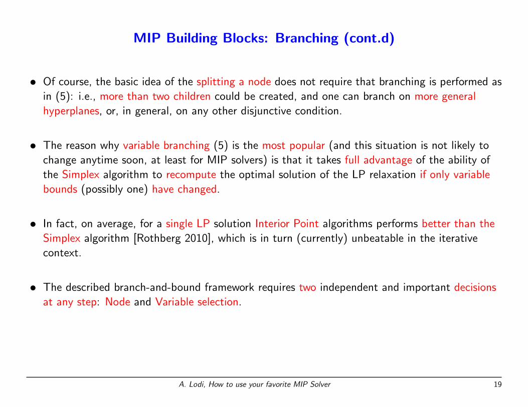
• In fact, on average, for a single LP solution Interior Point algorithms performs better than the
Simplex algorithm [Rothberg 2010], which is in turn (currently) unbeatable in the iterative
context.
A. Lodi, How to use your favorite MIP Solver 19
MIP Building Blocks: Branching (cont.d)
• Of course, the basic idea of the splitting a node does not require that branching is performed as
in (5): i.e., more than two children could be created, and one can branch on more general
hyperplanes, or, in general, on any other disjunctive condition.
• The reason why variable branching (5) is the most popular (and this situation is not likely to
change anytime soon, at least for MIP solvers) is that it takes full advantage of the ability of
the Simplex algorithm to recompute the optimal solution of the LP relaxation if only variable
bounds (possibly one) have changed.
• In fact, on average, for a single LP solution Interior Point algorithms performs better than the
Simplex algorithm [Rothberg 2010], which is in turn (currently) unbeatable in the iterative
context.
• The described branch-and-bound framework requires two independent and important decisions
at any step: Node and Variable selection.
A. Lodi, How to use your favorite MIP Solver 19
MIP Building Blocks: Branching (cont.d)
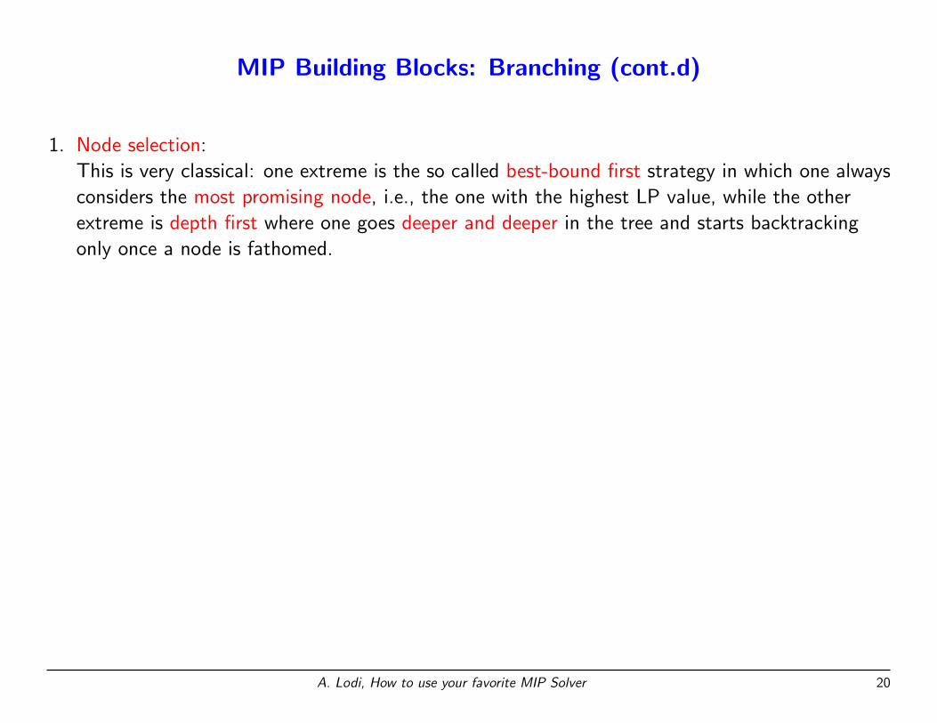
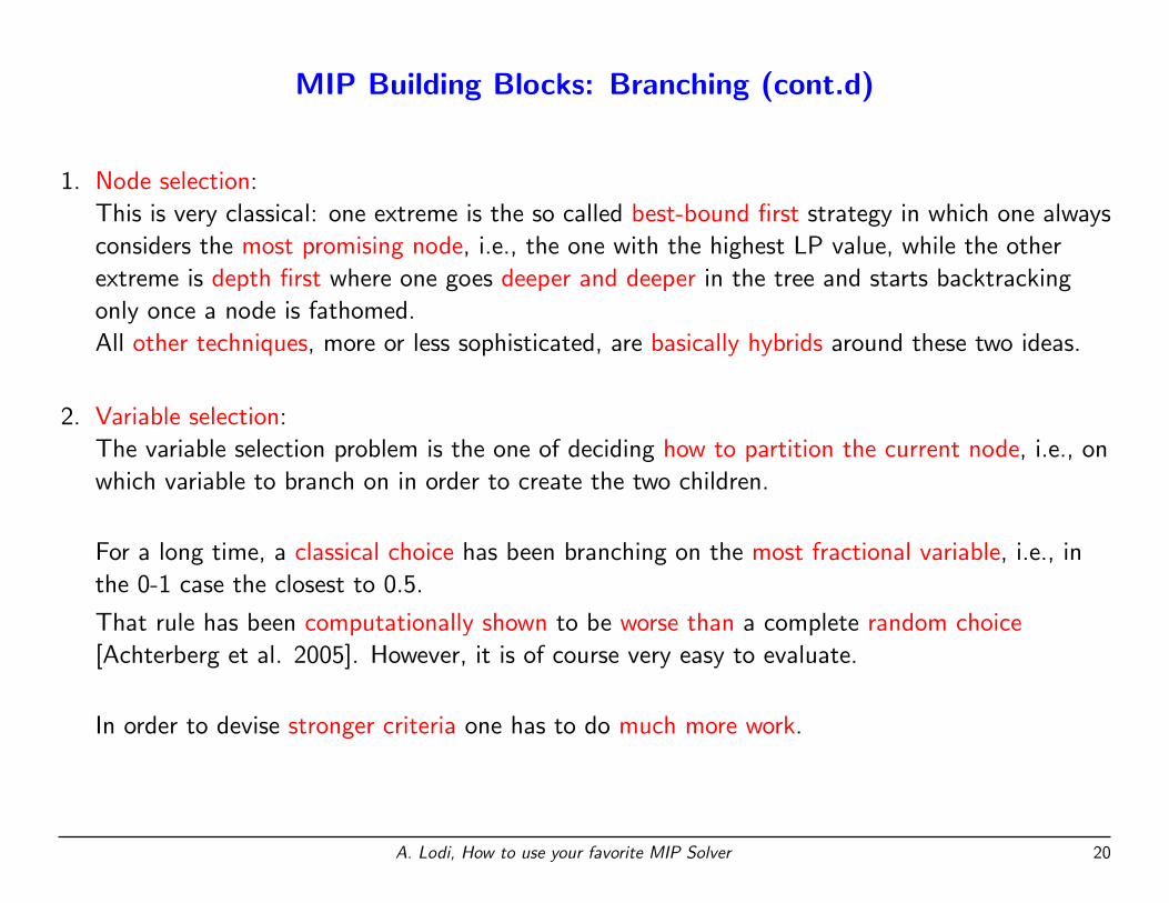
1. Node selection:
This is very classical: one extreme is the so called best-bound first strategy in which one always
considers the most promising node, i.e., the one with the highest LP value, while the other
extreme is depth first where one goes deeper and deeper in the tree and starts backtracking
only once a node is fathomed.
A. Lodi, How to use your favorite MIP Solver 20
MIP Building Blocks: Branching (cont.d)
1. Node selection:
This is very classical: one extreme is the so called best-bound first strategy in which one always
considers the most promising node, i.e., the one with the highest LP value, while the other
extreme is depth first where one goes deeper and deeper in the tree and starts backtracking
only once a node is fathomed.
All other techniques, more or less sophisticated, are basically hybrids around these two ideas.
2. Variable selection:
The variable selection problem is the one of deciding how to partition the current node, i.e., on
which variable to branch on in order to create the two children.
For a long time, a classical choice has been branching on the most fractional variable, i.e., in
the 0-1 case the closest to 0.5.
That rule has been computationally shown to be worse than a complete random choice
[Achterberg et al. 2005]. However, it is of course very easy to evaluate.
In order to devise stronger criteria one has to do much more work.
A. Lodi, How to use your favorite MIP Solver 20
MIP Building Blocks: Branching (cont.d)
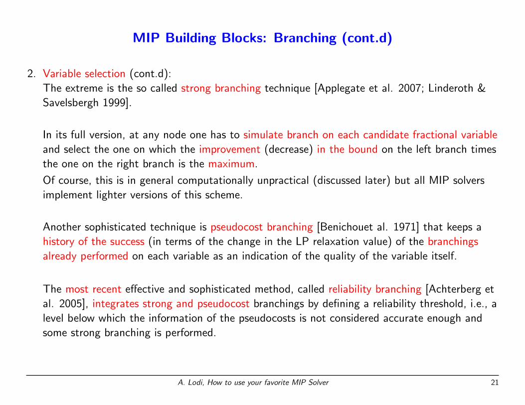
2. Variable selection (cont.d):
The extreme is the so called strong branching technique [Applegate et al. 2007; Linderoth &
Savelsbergh 1999].
A. Lodi, How to use your favorite MIP Solver 21
MIP Building Blocks: Branching (cont.d)
2. Variable selection (cont.d):
The extreme is the so called strong branching technique [Applegate et al. 2007; Linderoth &
Savelsbergh 1999].
In its full version, at any node one has to simulate branch on each candidate fractional variable
and select the one on which the improvement (decrease) in the bound on the left branch times
the one on the right branch is the maximum.
Of course, this is in general computationally unpractical (discussed later) but all MIP solvers
implement lighter versions of this scheme.
Another sophisticated technique is pseudocost branching [Benichouet al. 1971] that keeps a
history of the success (in terms of the change in the LP relaxation value) of the branchings
already performed on each variable as an indication of the quality of the variable itself.
The most recent effective and sophisticated method, called reliability branching [Achterberg et
al. 2005], integrates strong and pseudocost branchings by defining a reliability threshold, i.e., a
level below which the information of the pseudocosts is not considered accurate enough and
some strong branching is performed.
A. Lodi, How to use your favorite MIP Solver 21
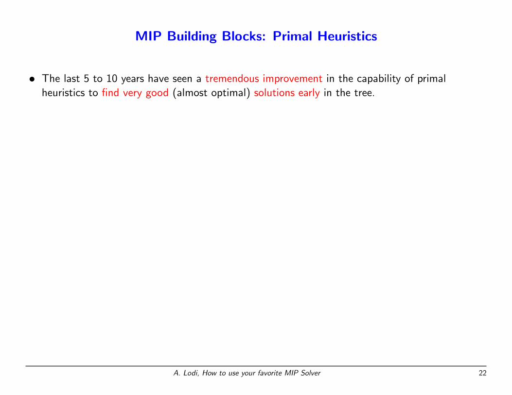
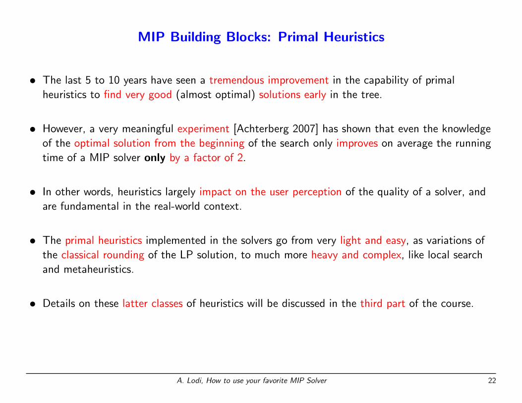
MIP Building Blocks: Primal Heuristics
• The last 5 to 10 years have seen a tremendous improvement in the capability of primal
heuristics to find very good (almost optimal) solutions early in the tree.
A. Lodi, How to use your favorite MIP Solver 22
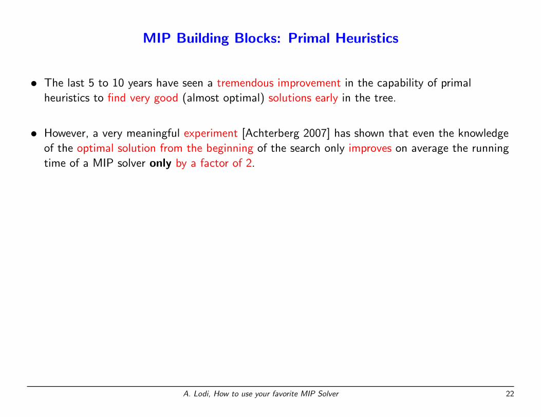
MIP Building Blocks: Primal Heuristics
• The last 5 to 10 years have seen a tremendous improvement in the capability of primal
heuristics to find very good (almost optimal) solutions early in the tree.
• However, a very meaningful experiment [Achterberg 2007] has shown that even the knowledge
of the optimal solution from the beginning of the search only improves on average the running
time of a MIP solver only by a factor of 2.
A. Lodi, How to use your favorite MIP Solver 22
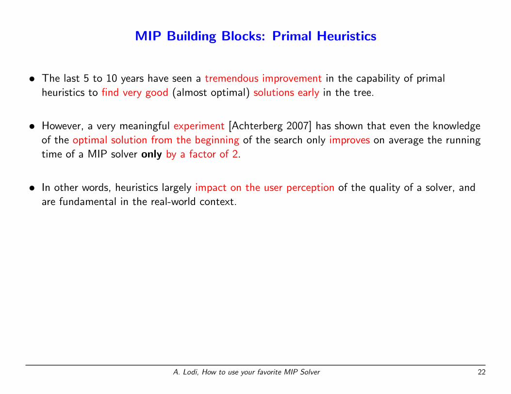
MIP Building Blocks: Primal Heuristics
• The last 5 to 10 years have seen a tremendous improvement in the capability of primal
heuristics to find very good (almost optimal) solutions early in the tree.
• However, a very meaningful experiment [Achterberg 2007] has shown that even the knowledge
of the optimal solution from the beginning of the search only improves on average the running
time of a MIP solver only by a factor of 2.
• In other words, heuristics largely impact on the user perception of the quality of a solver, and
are fundamental in the real-world context.
A. Lodi, How to use your favorite MIP Solver 22
MIP Building Blocks: Primal Heuristics
• The last 5 to 10 years have seen a tremendous improvement in the capability of primal
heuristics to find very good (almost optimal) solutions early in the tree.
• However, a very meaningful experiment [Achterberg 2007] has shown that even the knowledge
of the optimal solution from the beginning of the search only improves on average the running
time of a MIP solver only by a factor of 2.
• In other words, heuristics largely impact on the user perception of the quality of a solver, and
are fundamental in the real-world context.
• The primal heuristics implemented in the solvers go from very light and easy, as variations of
the classical rounding of the LP solution, to much more heavy and complex, like local search
and metaheuristics.
• Details on these latter classes of heuristics will be discussed in the third part of the course.
A. Lodi, How to use your favorite MIP Solver 22
MIP Solvers: exploiting multiple cores
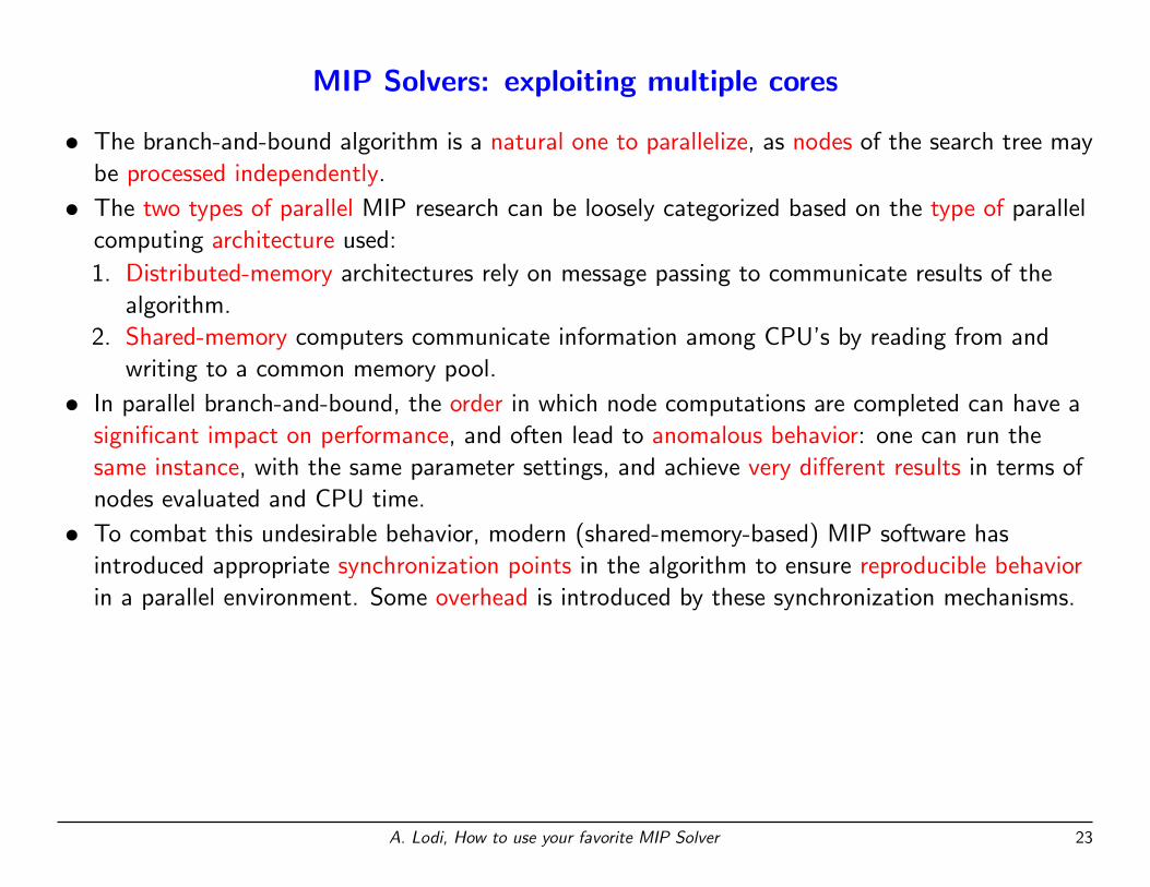
• The branch-and-bound algorithm is a natural one to parallelize, as nodes of the search tree may
be processed independently.
A. Lodi, How to use your favorite MIP Solver 23
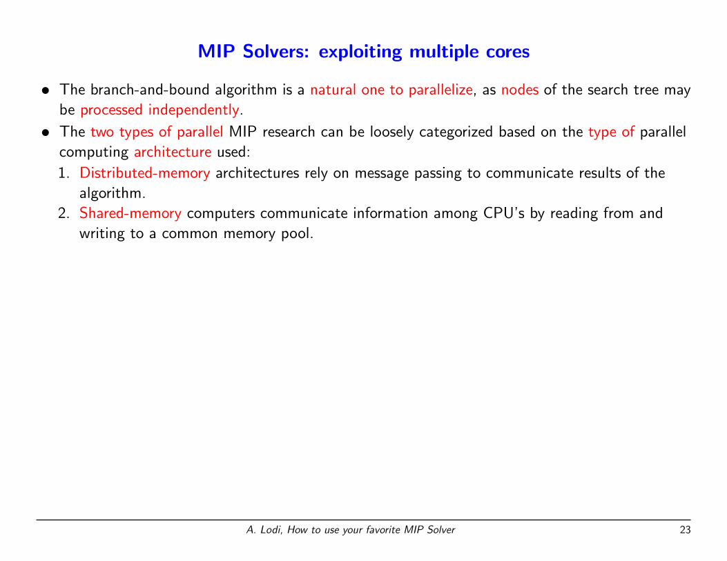
MIP Solvers: exploiting multiple cores
• The branch-and-bound algorithm is a natural one to parallelize, as nodes of the search tree may
be processed independently.
• The two types of parallel MIP research can be loosely categorized based on the type of parallel
computing architecture used:
1. Distributed-memory architectures rely on message passing to communicate results of the
algorithm.
2. Shared-memory computers communicate information among CPU’s by reading from and
writing to a common memory pool.
A. Lodi, How to use your favorite MIP Solver 23
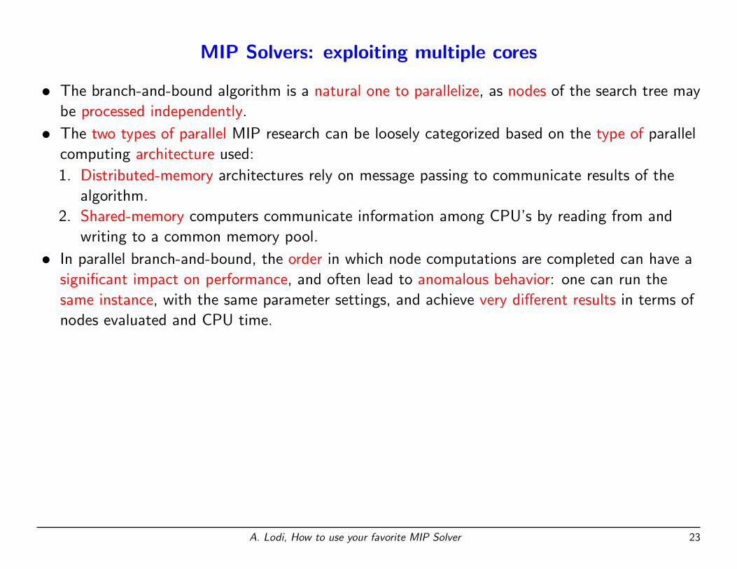
MIP Solvers: exploiting multiple cores
• The branch-and-bound algorithm is a natural one to parallelize, as nodes of the search tree may
be processed independently.
• The two types of parallel MIP research can be loosely categorized based on the type of parallel
computing architecture used:
1. Distributed-memory architectures rely on message passing to communicate results of the
algorithm.
2. Shared-memory computers communicate information among CPU’s by reading from and
writing to a common memory pool.
• In parallel branch-and-bound, the order in which node computations are completed can have a
significant impact on performance, and often lead to anomalous behavior: one can run the
same instance, with the same parameter settings, and achieve very different results in terms of
nodes evaluated and CPU time.
A. Lodi, How to use your favorite MIP Solver 23
MIP Solvers: exploiting multiple cores
• The branch-and-bound algorithm is a natural one to parallelize, as nodes of the search tree may
be processed independently.
• The two types of parallel MIP research can be loosely categorized based on the type of parallel
computing architecture used:
1. Distributed-memory architectures rely on message passing to communicate results of the
algorithm.
2. Shared-memory computers communicate information among CPU’s by reading from and
writing to a common memory pool.
• In parallel branch-and-bound, the order in which node computations are completed can have a
significant impact on performance, and often lead to anomalous behavior: one can run the
same instance, with the same parameter settings, and achieve very different results in terms of
nodes evaluated and CPU time.
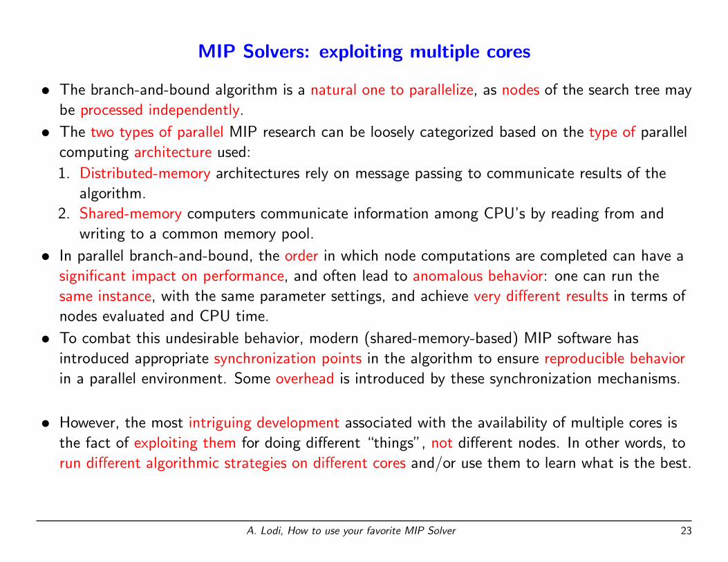
• To combat this undesirable behavior, modern (shared-memory-based) MIP software has
introduced appropriate synchronization points in the algorithm to ensure reproducible behavior
in a parallel environment. Some overhead is introduced by these synchronization mechanisms.
A. Lodi, How to use your favorite MIP Solver 23
MIP Solvers: exploiting multiple cores
• The branch-and-bound algorithm is a natural one to parallelize, as nodes of the search tree may
be processed independently.
• The two types of parallel MIP research can be loosely categorized based on the type of parallel
computing architecture used:
1. Distributed-memory architectures rely on message passing to communicate results of the
algorithm.
2. Shared-memory computers communicate information among CPU’s by reading from and
writing to a common memory pool.
• In parallel branch-and-bound, the order in which node computations are completed can have a
significant impact on performance, and often lead to anomalous behavior: one can run the
same instance, with the same parameter settings, and achieve very different results in terms of
nodes evaluated and CPU time.
• To combat this undesirable behavior, modern (shared-memory-based) MIP software has
introduced appropriate synchronization points in the algorithm to ensure reproducible behavior
in a parallel environment. Some overhead is introduced by these synchronization mechanisms.
• However, the most intriguing development associated with the availability of multiple cores is
the fact of exploiting them for doing different “things”, not different nodes. In other words, to
run different algorithmic strategies on different cores and/or use them to learn what is the best.
A. Lodi, How to use your favorite MIP Solver 23
MIP Evolution, a development viewpoint
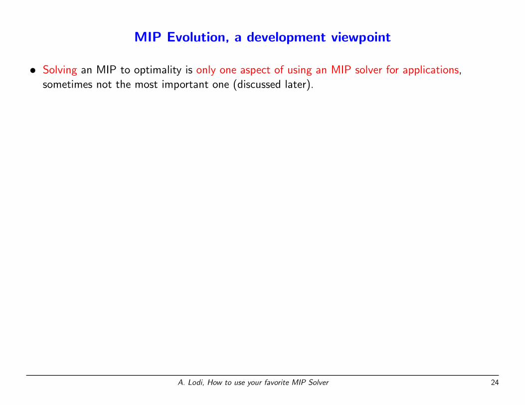
• Solving an MIP to optimality is only one aspect of using an MIP solver for applications,
sometimes not the most important one (discussed later).
A. Lodi, How to use your favorite MIP Solver 24
MIP Evolution, a development viewpoint
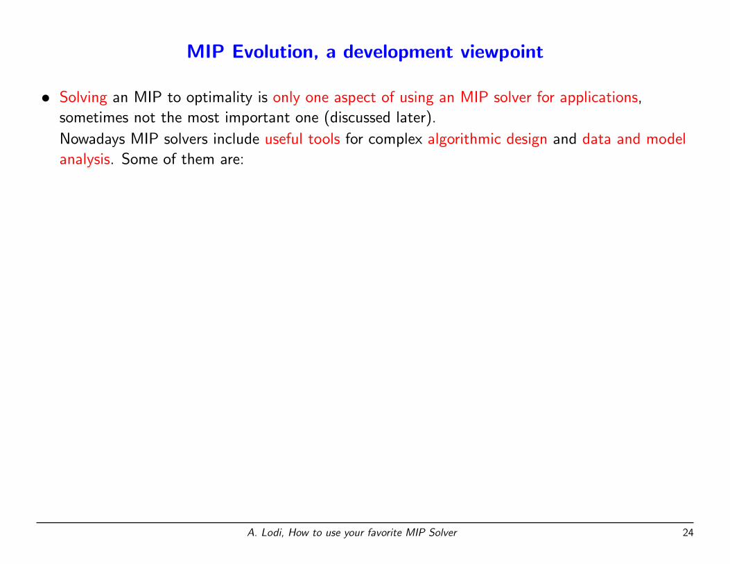
• Solving an MIP to optimality is only one aspect of using an MIP solver for applications,
sometimes not the most important one (discussed later).
Nowadays MIP solvers include useful tools for complex algorithmic design and data and model
analysis. Some of them are:
A. Lodi, How to use your favorite MIP Solver 24
MIP Evolution, a development viewpoint
• Solving an MIP to optimality is only one aspect of using an MIP solver for applications,
sometimes not the most important one (discussed later).
Nowadays MIP solvers include useful tools for complex algorithmic design and data and model
analysis. Some of them are:
– automatic tuning of the parameters:
the number of parameters (corresponding to different algorithmic options) makes the
hand-tuning complex but it guarantees great flexibility
– multiple solutions:
allow flexibility and support for decision making and, as side effect, improve primal heuristics
– detection of sources of infeasibility in the models:
real-world models are often over constrained and sources of infeasibility must be removed
[Amaldi et al. 2003; Chinneck 2001]
– callbacks:
allow flexibility to accommodate the user code so as to take advantage of specific knowledge
A. Lodi, How to use your favorite MIP Solver 24
MIP Software
• We have already discussed about the historical path that led to nowadays solvers.
A. Lodi, How to use your favorite MIP Solver 25
MIP Software
• We have already discussed about the historical path that led to nowadays solvers.
• An important aspect of the design of software for solving MIPs is the user interface. The range
of purposes for MIP software is quite large, thus the need of a large number of user interfaces.
• In general, users may wish
1. to solve MIPs using the solver as a “black box” (so-called interactive use),
2. to call the software from a third-party package (like a modeling language as AMPL), or
3. to embed the solver into custom applications, which would require software to have a
callable library.
• Finally, the user may wish to adapt certain aspects of the algorithm, and, as already discussed,
this can be achieved by callback functions, or, when the source code is available, through
abstract interfaces.
A. Lodi, How to use your favorite MIP Solver 25
MIP Commercial Software
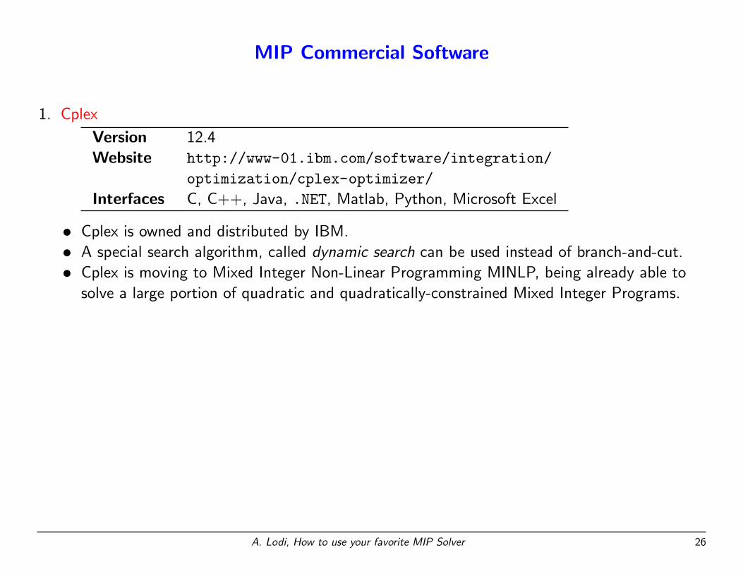
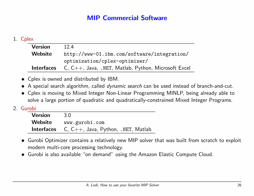
1. Cplex
Version 12.4
Website http://www-01.ibm.com/software/integration/
optimization/cplex-optimizer/
Interfaces C, C++, Java, .NET, Matlab, Python, Microsoft Excel
• Cplex is owned and distributed by IBM.
• A special search algorithm, called dynamic search can be used instead of branch-and-cut.
• Cplex is moving to Mixed Integer Non-Linear Programming MINLP, being already able to
solve a large portion of quadratic and quadratically-constrained Mixed Integer Programs.
A. Lodi, How to use your favorite MIP Solver 26
MIP Commercial Software
1. Cplex
Version 12.4
Website http://www-01.ibm.com/software/integration/
optimization/cplex-optimizer/
Interfaces C, C++, Java, .NET, Matlab, Python, Microsoft Excel
• Cplex is owned and distributed by IBM.
• A special search algorithm, called dynamic search can be used instead of branch-and-cut.
• Cplex is moving to Mixed Integer Non-Linear Programming MINLP, being already able to
solve a large portion of quadratic and quadratically-constrained Mixed Integer Programs.
2. GurobiVersion 3.0
Website www.gurobi.com
Interfaces C, C++, Java, Python, .NET, Matlab
• Gurobi Optimizer contains a relatively new MIP solver that was built from scratch to exploit
modern multi-core processing technology.
• Gurobi is also available “on demand” using the Amazon Elastic Compute Cloud.
A. Lodi, How to use your favorite MIP Solver 26
MIP Commercial Software (cont.d)
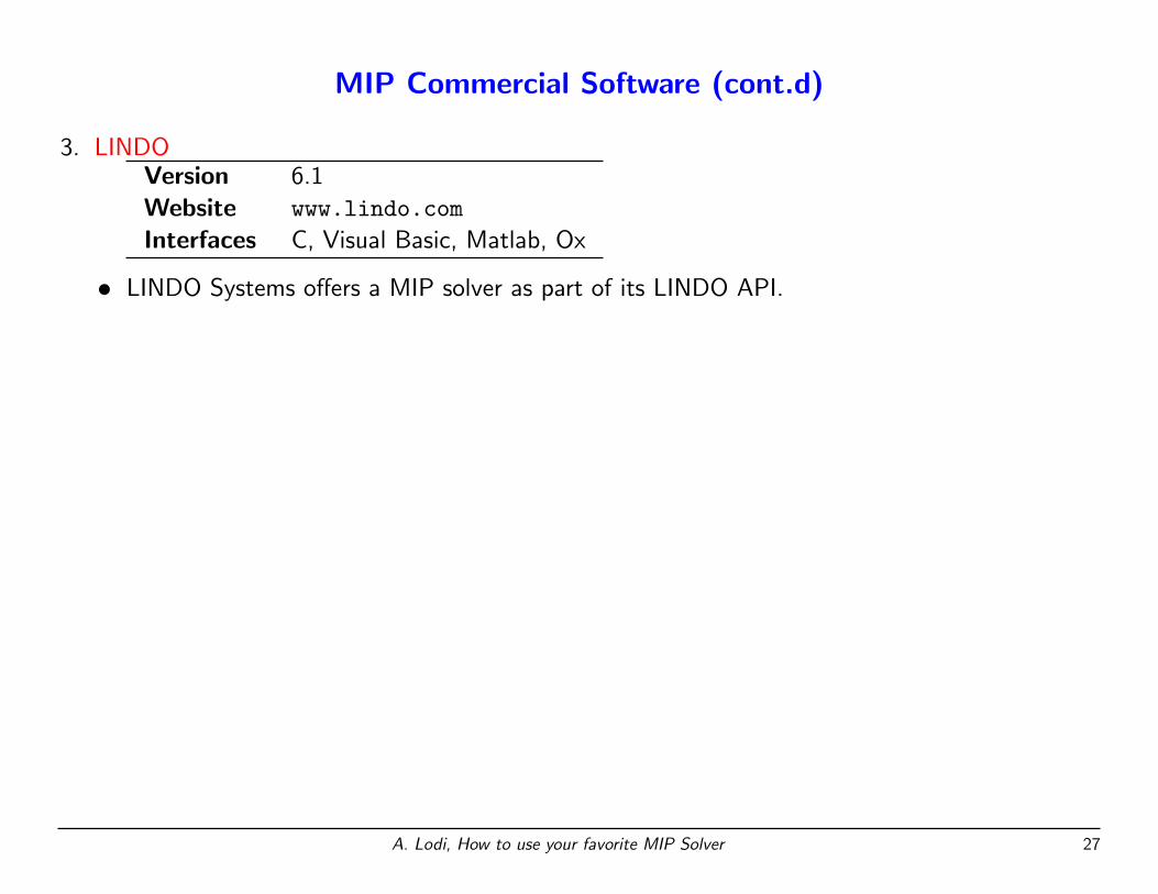
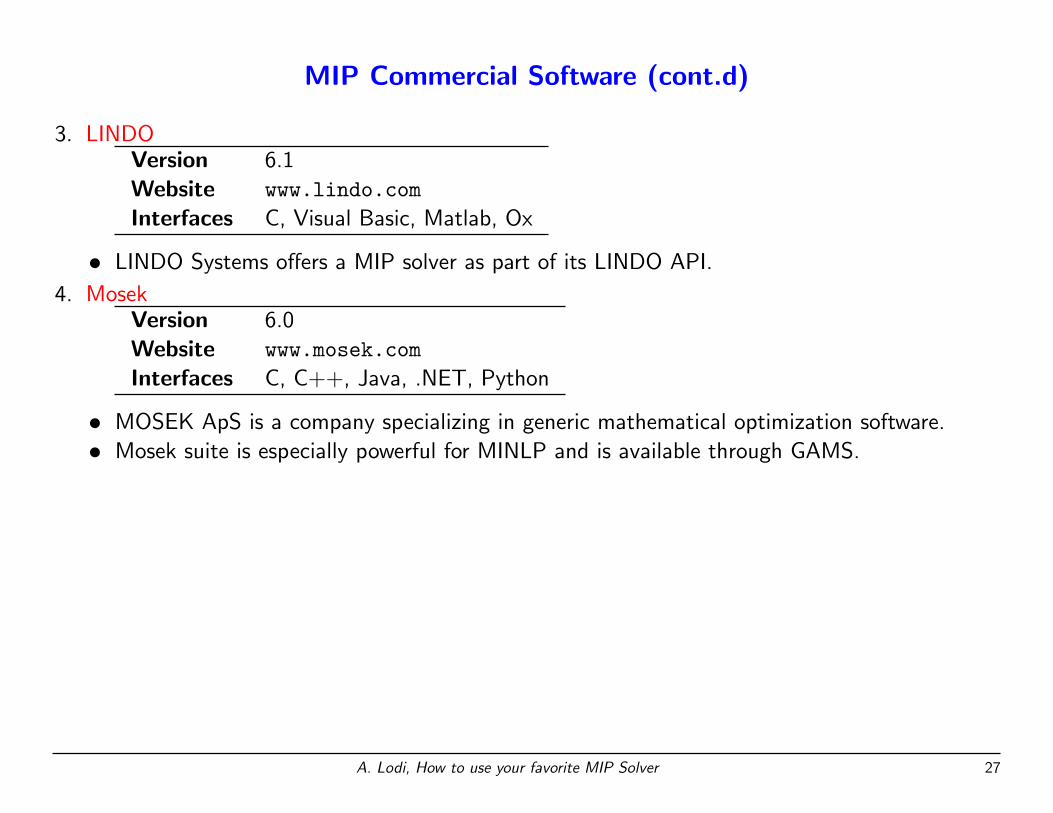
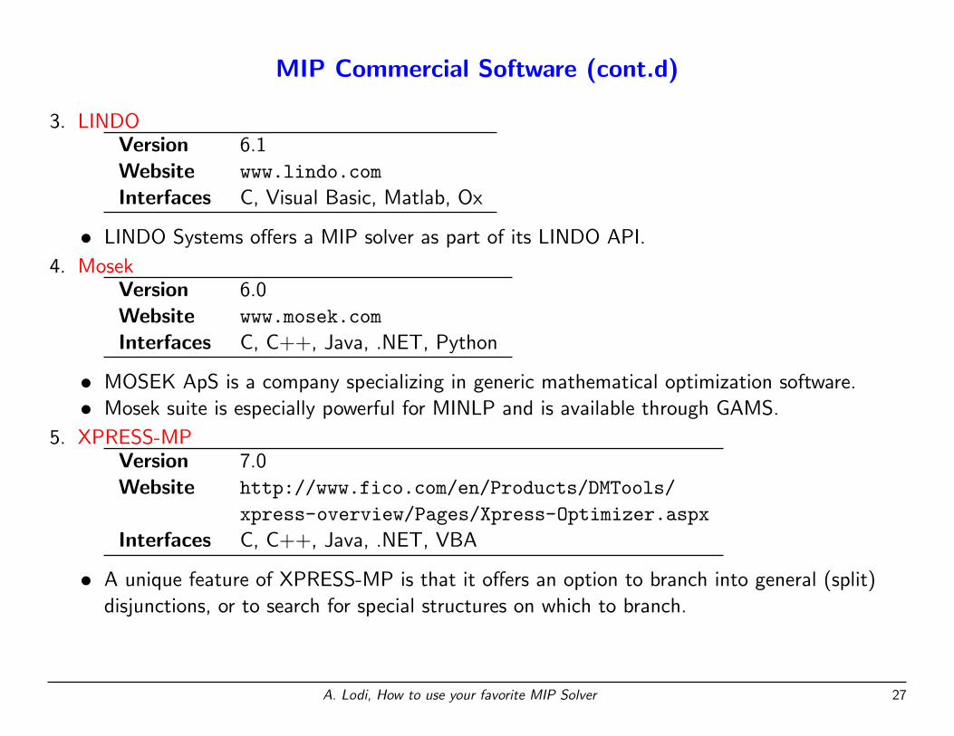
3. LINDOVersion 6.1
Website www.lindo.com
Interfaces C, Visual Basic, Matlab, Ox
• LINDO Systems offers a MIP solver as part of its LINDO API.
A. Lodi, How to use your favorite MIP Solver 27
MIP Commercial Software (cont.d)
3. LINDOVersion 6.1
Website www.lindo.com
Interfaces C, Visual Basic, Matlab, Ox
• LINDO Systems offers a MIP solver as part of its LINDO API.
4. MosekVersion 6.0
Website www.mosek.com
Interfaces C, C++, Java, .NET, Python
• MOSEK ApS is a company specializing in generic mathematical optimization software.
• Mosek suite is especially powerful for MINLP and is available through GAMS.
5. XPRESS-MPVersion 7.0
Website http://www.fico.com/en/Products/DMTools/
xpress-overview/Pages/Xpress-Optimizer.aspx
Interfaces C, C++, Java, .NET, VBA
• A unique feature of XPRESS-MP is that it offers an option to branch into general (split)
disjunctions, or to search for special structures on which to branch.
A. Lodi, How to use your favorite MIP Solver 27
MIP Noncommercial Software
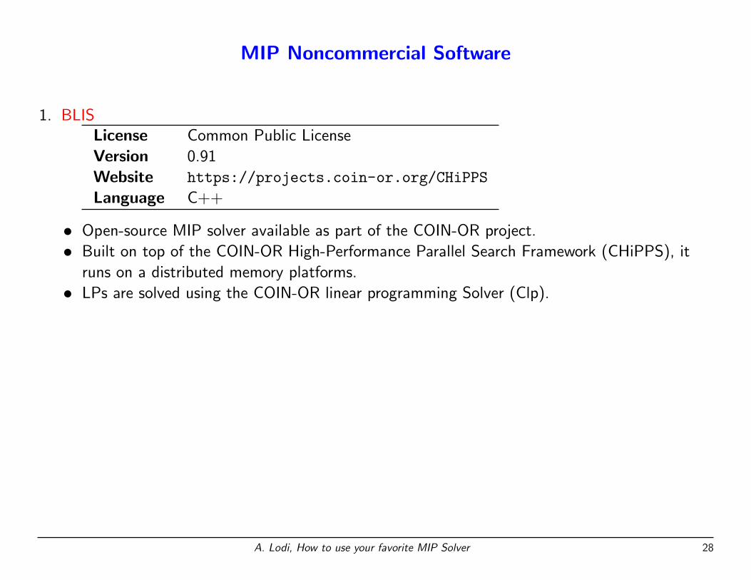
1. BLISLicense Common Public License
Version 0.91
Website https://projects.coin-or.org/CHiPPS
Language C++
• Open-source MIP solver available as part of the COIN-OR project.
• Built on top of the COIN-OR High-Performance Parallel Search Framework (CHiPPS), it
runs on a distributed memory platforms.
• LPs are solved using the COIN-OR linear programming Solver (Clp).
A. Lodi, How to use your favorite MIP Solver 28
MIP Noncommercial Software
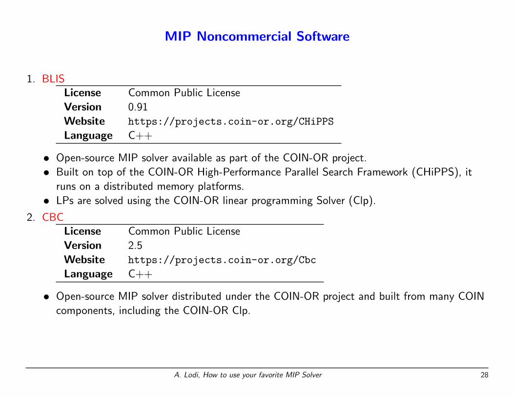
1. BLISLicense Common Public License
Version 0.91
Website https://projects.coin-or.org/CHiPPS
Language C++
• Open-source MIP solver available as part of the COIN-OR project.
• Built on top of the COIN-OR High-Performance Parallel Search Framework (CHiPPS), it
runs on a distributed memory platforms.
• LPs are solved using the COIN-OR linear programming Solver (Clp).
2. CBCLicense Common Public License
Version 2.5
Website https://projects.coin-or.org/Cbc
Language C++
• Open-source MIP solver distributed under the COIN-OR project and built from many COIN
components, including the COIN-OR Clp.
A. Lodi, How to use your favorite MIP Solver 28
MIP Noncommercial Software (cont.d)
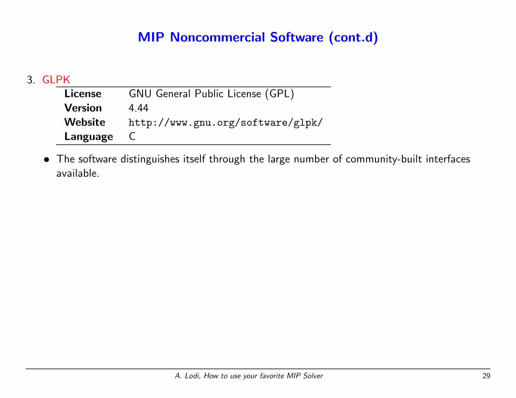
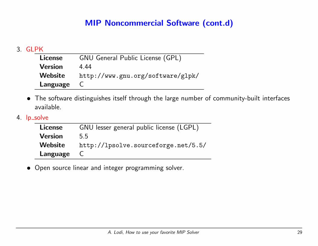
3. GLPKLicense GNU General Public License (GPL)
Version 4.44
Website http://www.gnu.org/software/glpk/
Language C
• The software distinguishes itself through the large number of community-built interfaces
available.
A. Lodi, How to use your favorite MIP Solver 29
MIP Noncommercial Software (cont.d)
3. GLPKLicense GNU General Public License (GPL)
Version 4.44
Website http://www.gnu.org/software/glpk/
Language C
• The software distinguishes itself through the large number of community-built interfaces
available.
4. lp solve
License GNU lesser general public license (LGPL)
Version 5.5
Website http://lpsolve.sourceforge.net/5.5/
Language C
• Open source linear and integer programming solver.
A. Lodi, How to use your favorite MIP Solver 29
MIP Noncommercial Software (cont.d)
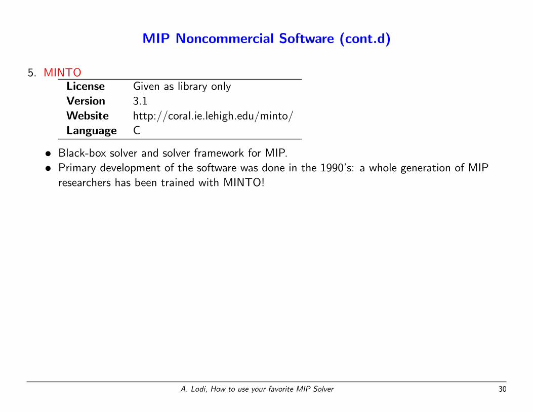
5. MINTOLicense Given as library only
Version 3.1
Website http://coral.ie.lehigh.edu/minto/
Language C
• Black-box solver and solver framework for MIP.
• Primary development of the software was done in the 1990’s: a whole generation of MIP
researchers has been trained with MINTO!
A. Lodi, How to use your favorite MIP Solver 30

MIP Noncommercial Software (cont.d)
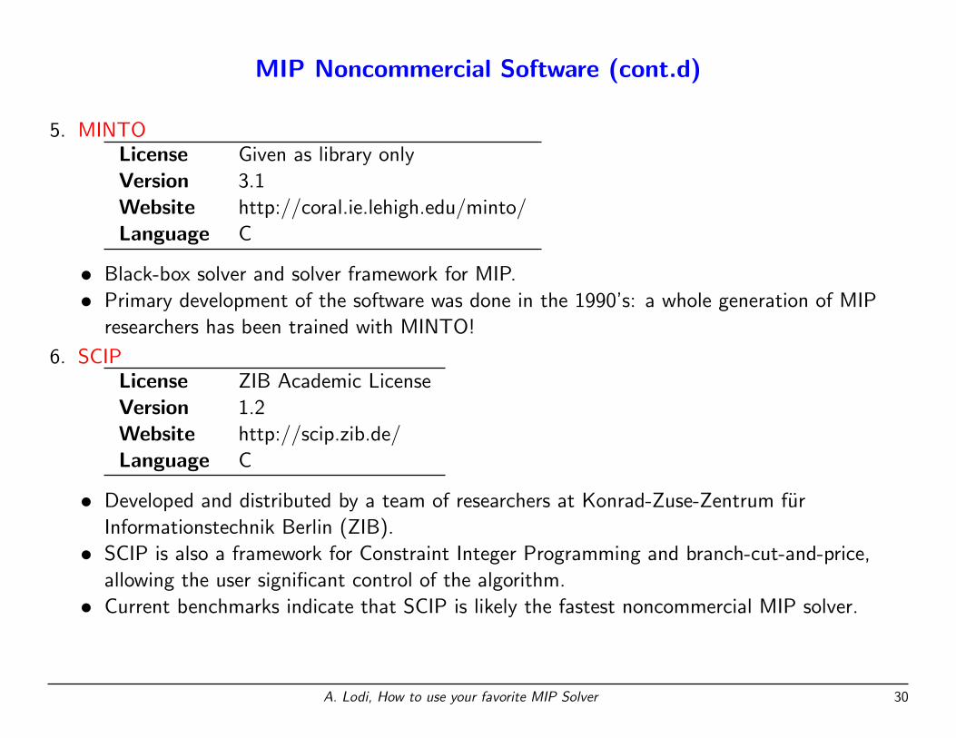
5. MINTOLicense Given as library only
Version 3.1
Website http://coral.ie.lehigh.edu/minto/
Language C
• Black-box solver and solver framework for MIP.
• Primary development of the software was done in the 1990’s: a whole generation of MIP
researchers has been trained with MINTO!
6. SCIPLicense ZIB Academic License
Version 1.2
Website http://scip.zib.de/
Language C
• Developed and distributed by a team of researchers at Konrad-Zuse-Zentrum fur
Informationstechnik Berlin (ZIB).
• SCIP is also a framework for Constraint Integer Programming and branch-cut-and-price,
allowing the user significant control of the algorithm.
• Current benchmarks indicate that SCIP is likely the fastest noncommercial MIP solver.
A. Lodi, How to use your favorite MIP Solver 30
MIP Noncommercial Software (cont.d)
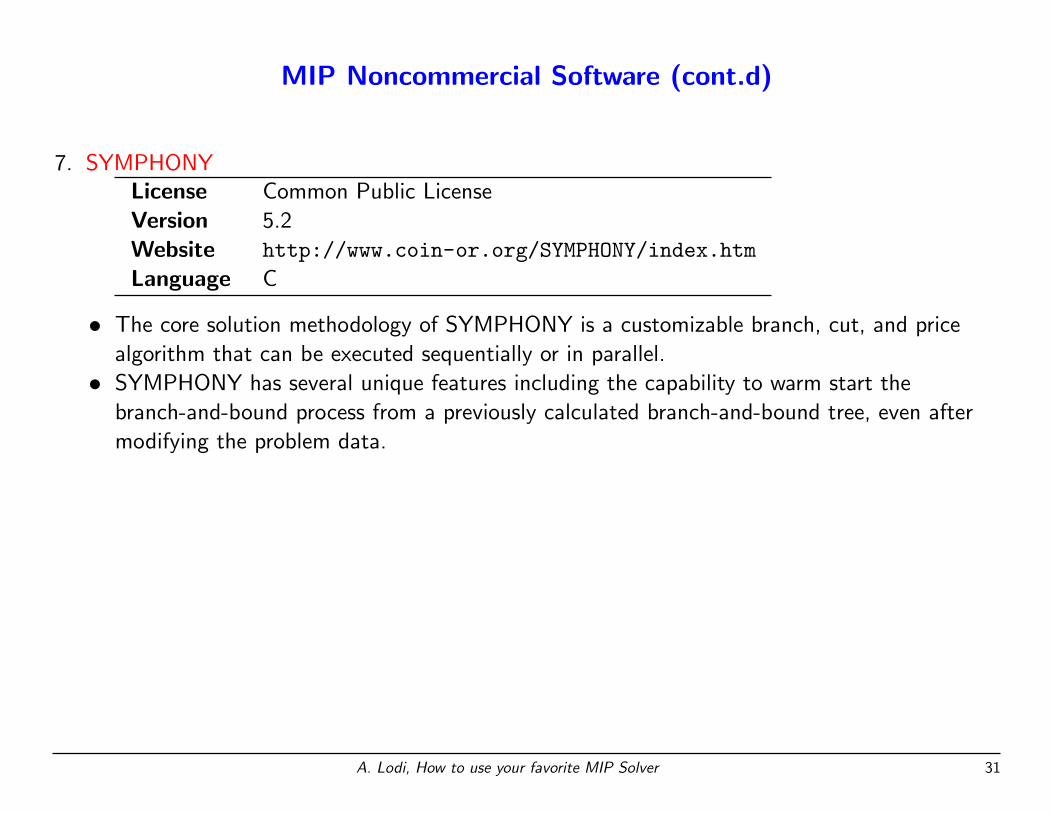
7. SYMPHONYLicense Common Public License
Version 5.2
Website http://www.coin-or.org/SYMPHONY/index.htm
Language C
• The core solution methodology of SYMPHONY is a customizable branch, cut, and price
algorithm that can be executed sequentially or in parallel.
• SYMPHONY has several unique features including the capability to warm start the
branch-and-bound process from a previously calculated branch-and-bound tree, even after
modifying the problem data.
A. Lodi, How to use your favorite MIP Solver 31
MIP Software: further remarks/pointers
• Any review of software features is inherently limited by the temporal nature of software itself.
A. Lodi, How to use your favorite MIP Solver 32
MIP Software: further remarks/pointers
• Any review of software features is inherently limited by the temporal nature of software itself.
• Many of the commercial packages have free or limited cost licensing options for academics.
A. Lodi, How to use your favorite MIP Solver 32
MIP Software: further remarks/pointers
• Any review of software features is inherently limited by the temporal nature of software itself.
• Many of the commercial packages have free or limited cost licensing options for academics.
• Hans Mittelmann has for many years run independent benchmarks of MIP software, and been
publishing the results. In general, the commercial software significantly outperforms
noncommercial software, but no conclusion is possible on the relative performance of different
commercial systems. See http://plato.asu.edu/ftp/milpf.html.
• The most recent version of MIP library, MIPLIB 2010 http://miplib.zib.de/, not only
provides problems and data, but it includes, for the first time, scripts to run automated tests in
a predefined way, and a solution checker to test the accuracy of provided solutions using exact
arithmetic [Koch et al. 2011].
• NEOS, server for optimization www-neos.mcs.anl.gov/neos: A user can submit an
optimization problem to the server and obtain the solution and running time statistics using the
preferred solver through different interfaces.
• COIN-OR http://www.coin-or.org: COmputational INfrastructure for Operations Research.
A. Lodi, How to use your favorite MIP Solver 32