How the Pandemic Taught Us to Turn Smart Beta into Real Alpha

How the Pandemic Taught Us to Turn Smart Beta into Real AlphaAs published in Journal of Asset Management December 2020

Dan diBartolomeo and Chris KantosSpaulding Group

PMAR June 2021

www.northinfo.com Slide 2

Introduction

• The ongoing coronavirus pandemic has strongly reminded equity investors that rare but extreme events occur from time to time. These events represent periods of increased volatility and in some cases very negative returns for extended periods.

•

• In this presentation we will examine how including the potential for such large events changes traditional views of equity returns and the known factors that contribute to those returns.

• By incorporating the probability of such rare events in factor models we conclude that strategies that focus on “alpha” (risk adjusted return) as defined in Jensen (1968) are structurally superior to “smart beta” strategies that attempt to outperform an equity index by active exposure to one or more known factors.

– Northfield US Fundamental Model is close enough in structure to provide persuasive empirical evidence.


Historical Features We Want to Explain

• The equity risk premium (return of equities minus the risk free rate) is widely considered to the unexpectedly high.

– This has lead some researchers to argue that long term investors should always be fully invested in equities (e.g. Siegel, 2014, Stocks for the Long Run)

• There has been widespread criticism of the mostly widely known asset pricing model, the CAPM (Sharpe, 1964) as failing to describe equity asset returns.

– The amount of return associated with low beta stocks versus high beta stocks seems inconsistent with the Sharpe version of CAPM.

• There is a massive literature of “factor anomalies” that describe persistent excess returns associated with security attributes in violation of the “Efficient Markets Hypothesis” (Fama, 1970).

– Value, Momentum, Size, Low Volatility


Distinct Semantics of Factor Returns

• The first distinction is the difference between “excess return” and “alpha”.

– “Excess return” outcomes that outperform some passive benchmark.

– “Alpha” to describe investment outcomes that outperform the some expected return associated with risk

• The second distinction is whether we estimate the return outcomes in a simple or orthogonal fashion.

– Factor outcomes can be simple: compare returns on a large cap portfolio and a small cap portfolio, as a “size” factor.

– Those two portfolios will have lots of other differences (e.g. average P/E) so we can’t be sure that return actually arise from “size”

– Statistical techniques can be used to control for correlated variables.

– We will always refer to orthogonalized values so we are describing returns associated with factors on a ceteris paribus basis.


Capital Asset Pricing Model (Sharpe, 1964)

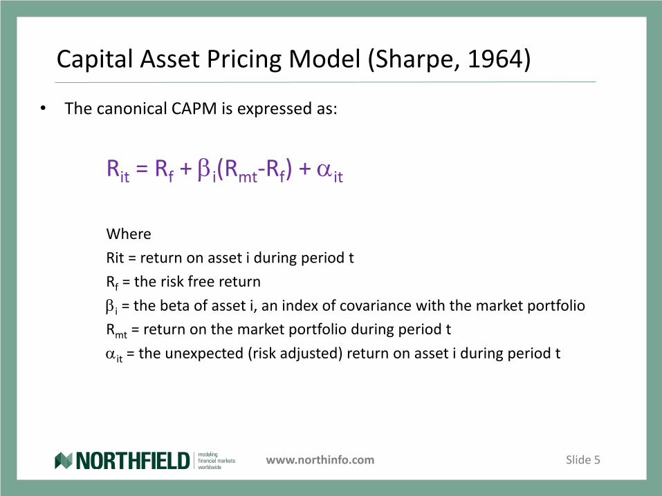
• The canonical CAPM is expressed as:

Rit = Rf + bi(Rmt-Rf) + ait

Where

Rit = return on asset i during period t

Rf = the risk free return

bi = the beta of asset i, an index of covariance with the market portfolio

Rmt = return on the market portfolio during period t

ait = the unexpected (risk adjusted) return on asset i during period t


Criticism of CAPM

• Numerous studies have argued the many unrealistic assumptions that are embedded in the original CAPM

– Single period model. Ignores compounding of returns

– Investors are assumed to borrow and lend at the risk free rate

– No limitations on investor leverage

– The “market portfolio” is well defined

– No transaction costs or taxes

– Beta values are known not estimated

• The major criticism is that empirical data suggests that the slope of the security market line is much less than (Rmt-Rf).

– The many critiques are summarized in Grinold (1992)

– Critiques are about expected returns, not about beta as a risk measure

– After 56 years, nobody has come up with a more widely accepted alternative


An Explanation of the Flatter SML

• Northfield has previously proposed explanations of the flatter SML

– These were covered in https://www.northinfo.com/documents/575.pdf.

– Various “fixes” are proposed for:

– The lack of compounding in the single period assumption

– The poor specification of the market portfolio

– The assumption of guaranteed survival (no bankruptcy)

– Use of estimates rather than known values for beta.

• The “fixes” individually and in aggregate suggest a flatter SML

• Uniquely, we assert that the SML is not a line at all but a curve which curves downward past a critical value we call “beta*”

– The SML curve is upward sloping for beta < beta*

– The SML curve is downward sloping for beta > beta*

https://www.northinfo.com/documents/575.pdf


Other Versions of CAPM

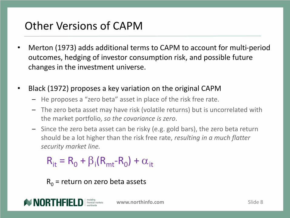
• Merton (1973) adds additional terms to CAPM to account for multi-period outcomes, hedging of investor consumption risk, and possible future changes in the investment universe.

• Black (1972) proposes a key variation on the original CAPM

– He proposes a “zero beta” asset in place of the risk free rate.

– The zero beta asset may have risk (volatile returns) but is uncorrelated with the market portfolio, so the covariance is zero.

– Since the zero beta asset can be risky (e.g. gold bars), the zero beta return should be a lot higher than the risk free rate, resulting in a much flatter security market line.

Rit = R0 + bi(Rmt-R0) + ait

R0 = return on zero beta assets


CAPM is Derived from Markowitz MPT

• With some additional assumptions, the CAPM can be derived MPT (Markowitz, 1952)

– This means that CAPM also embeds some of the assumptions of MPT including that the security returns are effectively random walk where portfolio returns are normally distributed and serially uncorrelated.

• Long term studies of equity returns such as Dimson, Marsh and Staunton (2014) illustrate that this assumption confounded by rare but large events.

– At the global level we might consider World War I, the Spanish Flu pandemic (1918), the 1929 Crash and subsequent Great Depression, World War II, the Global Financial Crisis (2007-2010), and the current Coronavirus pandemic. Six “large” events over roughly a century.

– There are numerous example of national financial collapse such as Russia (1917), Germany (1930s) China (1948), Mexico (1982), Russia (1997), Zimbabwe (2008), Venezuela (now)


Catastrophe Bonds and Lottery Tickets

• One way to reconcile the CAPM and with the existence of rare, but large events is to think of investors being long the equity market and a short a lottery ticket where they randomly sustain large losses.

– Similar to the concept of catastrophe bonds in fixed income

• Since the rare events are rare and random, the expectation of the correlation between lottery payoffs and the market is zero.

– Our very risky position in lottery tickets therefore has zero beta

– Barro (2005) and Gabaix (2009) argue that investors are aware of the potential for rare, large losses and demand a high equity risk premium.

– If the implicit “catastrophe loss” asset is unavoidably built into an investor’s market exposure, this qualifies under Black version of CAPM as the zero beta risky asset.

– The expectation of rare, large losses implies that the expected distribution of equity market returns will have negative skew and positive excess kurtosis over finite intervals.


Patching CAPM for Higher Moments

• A common approach to reconciling return distributions with higher moments when they are assumed to be normal is the method of Cornish and Fisher (1937)

• Essentially we adjust the expected volatility of the market portfolio to account for the effects of skew and kurtosis.

– For example, consider an asset 8% expected return with an estimated annual volatility of 10% under the normal distribution assumption.

– If we assume a 6% annual likelihood of a 50% loss, the expected return drops to 5.2% and effective volatility of this asset goes from 10% to 23%.

• It should follow that investors will demand additional return compensation for the lost return and increased risk, increasing the magnitude of the portion of equity risk premium (Rmt- Rf) that is attributable to R0t and reducing the slope of the SML (Rmt- R0t)


The Answer is Always Six

• There are three components of the expectation of R0

• The first is the time value of money, Rf

• The second is the change in the expected mean of the distribution

– In our previous example, (8-5.2) = 2.8%

• The third is incremental return that investors will demand for the increase in effective volatility

– In the example, the expectation of the incremental return is (23-10)/6 = 2.16%

– For our hypothetical, the effect of including our “short lottery ticket” is 4.96%, a large fraction of usual expectations of the equity risk premium

– The rationale for the denominator of six was explained in a recent webinar, https://www.northinfo.com/Documents/939.pdf

https://www.northinfo.com/Documents/939.pdf


An Alternative Approach

• Harvey and Siddique (2000) studies the impact of “co-skewness” across securities on asset pricing models.

• It considers how much a particular security contributes to the skewness of a broad portfolio.

– In a large market decline driven by the onset of war, some equities would might be hurt a lot while other might actually prosper (e.g. defense contractors).

– In the GFC, financial stocks were particularly impacted

– In the coronavirus pandemic, airlines and hotels have been most strongly impacted, while many tech firms and pharma companies have done well.

• They conclude that the collective impact of “co-skewness” is on the order of 3.6% return per annum on a typical market index portfolio.

– “In the ballpark” of our estimate of the components of R0


Bankruptcy Risk

• Bankruptcies at the individual firm level are obviously more likely during periods of market stress. The correlation across failures is a major source of “co-skewness”

– The CAPM assumes that bankruptcies do not exist.

– Merton (1974) shows that bankruptcy risk can described as an option where the volatility of a firm’s asset value is the key input.

– diBartolomeo (JOI, 2010) shows that asset volatility is approximately equal to equity volatility divided by the firm’s debt/equity ratio

– Several studies have shown that the excess return associated with successfully avoiding bankruptcies is on the order of 3% per annum. https://www.northinfo.com/Documents/848.pdf

• If total volatility contributes to bankruptcy losses, but the return associated with beta risk is upward sloping (positive SML) then the return from idiosyncratic risk at the firm level must be negative, while CAPM assumes zero.

https://www.northinfo.com/Documents/848.pdf


Northfield US Fundamental Model

• For empirical analysis of the our ideas, we can use the Northfield US Fundamental Model.

– There is a large sample of data history extending back to January 1989. Analytical changes to the model have been minimal (we got it right the first time) and do not effect this analysis.

– ADRs are included to give some coverage of global equities

– The model is based in the class CAPM, with the alpha term subdivided into 66 “factor alphas” (11 unit normal style factors and 55 industries)

– Estimation of the factor beta and factor alpha is weighted by the square root of capitalization which affords a balance between the influence of large cap stocks and the more numerous small cap stocks. As noted in Grinold and Kahn (1995), there are also desirable statistical properties to this concept.

– One of the “style factors” is a rescaled range measure of total volatility which we will use as our proxy for bankruptcy risk and thus likely contribution to the existence of higher moments in the market portfolio.


Fundamental Model Formulation

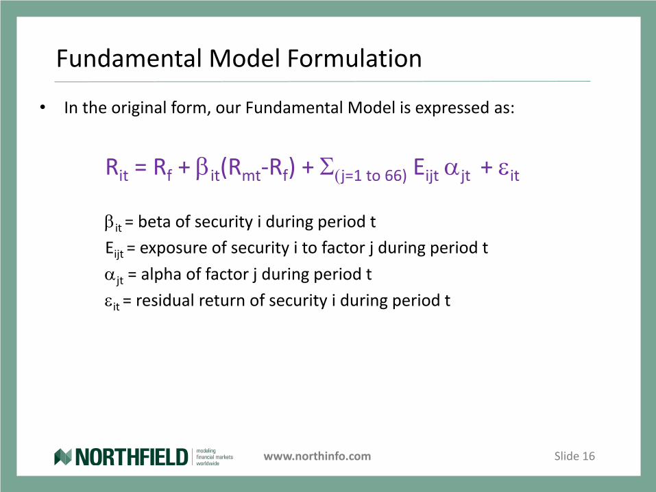
• In the original form, our Fundamental Model is expressed as:

Rit = Rf + bit(Rmt-Rf) + S(j=1 to 66) Eijt ajt + eit

bit = beta of security i during period t

Eijt = exposure of security i to factor j during period t

ajt = alpha of factor j during period t

eit = residual return of security i during period t


Reordered US Fundamental Model

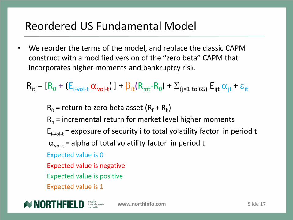
• We reorder the terms of the model, and replace the classic CAPM construct with a modified version of the “zero beta” CAPM that incorporates higher moments and bankruptcy risk.

Rit = [R0 + (Ei-vol-t avol-t) ] + bit(Rmt-R0) + S(j=1 to 65) Eijt ajt + eit

R0 = return to zero beta asset (Rf + Rh)

Rh = incremental return for market level higher moments

Ei-vol-t = exposure of security i to total volatility factor in period t

avol-t = alpha of total volatility factor in period t

Expected value is 0

Expected value is negative

Expected value is positive

Expected value is 1


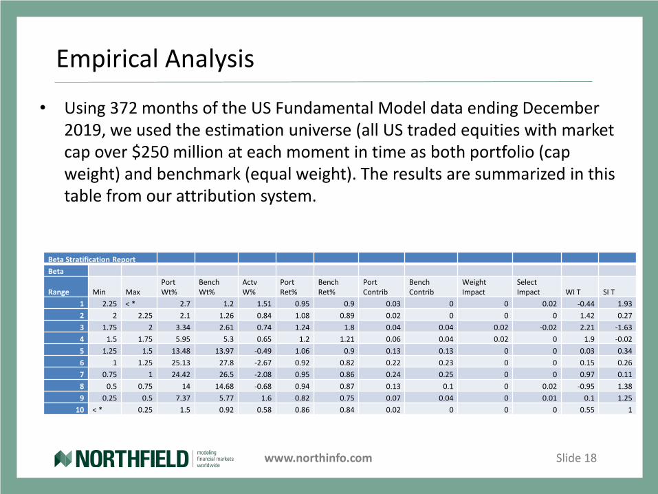
Empirical Analysis

• Using 372 months of the US Fundamental Model data ending December 2019, we used the estimation universe (all US traded equities with market cap over $250 million at each moment in time as both portfolio (cap weight) and benchmark (equal weight). The results are summarized in this table from our attribution system.

Beta Stratification Report

Beta

Range Min MaxPort Wt%

Bench Wt%

Actv W%

Port Ret%

Bench Ret%

Port Contrib

Bench Contrib

Weight Impact

Select Impact WI T SI T

1 2.25 < * 2.7 1.2 1.51 0.95 0.9 0.03 0 0 0.02 -0.44 1.93

2 2 2.25 2.1 1.26 0.84 1.08 0.89 0.02 0 0 0 1.42 0.27

3 1.75 2 3.34 2.61 0.74 1.24 1.8 0.04 0.04 0.02 -0.02 2.21 -1.63

4 1.5 1.75 5.95 5.3 0.65 1.2 1.21 0.06 0.04 0.02 0 1.9 -0.02

5 1.25 1.5 13.48 13.97 -0.49 1.06 0.9 0.13 0.13 0 0 0.03 0.34

6 1 1.25 25.13 27.8 -2.67 0.92 0.82 0.22 0.23 0 0 0.15 0.26

7 0.75 1 24.42 26.5 -2.08 0.95 0.86 0.24 0.25 0 0 0.97 0.11

8 0.5 0.75 14 14.68 -0.68 0.94 0.87 0.13 0.1 0 0.02 -0.95 1.38

9 0.25 0.5 7.37 5.77 1.6 0.82 0.75 0.07 0.04 0 0.01 0.1 1.25

10 < * 0.25 1.5 0.92 0.58 0.86 0.84 0.02 0 0 0 0.55 1


Empirical Analysis Discussion

• Using the data which underlies the table we are able to estimate the key parameters of the “reordered” Fundamental Model

– There is positive correlation between beta values and portfolio returns on both a cap weighted (.41) and equal weighted (.61) basis. Both produce SML slopes (Rm-R0)around +1.6% per annum, with T-stats of 3 and 3.6 respectively.

– Pooling results in a slope of 1.8% with a T-Stat of 4

– The average value of Rh (risk premium for rare, large events) is .39% per month or about 4.7% per annum, close to values from our hypothetical and Harvey and Siddique (3.6 for skew only)

– The times series average factor alpha to total volatility is -.20% per month, in line with our expectation of bankruptcy losses in equities with higher idiosyncratic risk.

– If we bifurcate the universe into “high vol” and “low vol” groups the resultant factor active factor exposure is consistent with the 3% excess return for bankruptcy avoidance.


Discussion of Other Factor Alphas

• The foregoing suggests a robust representation of the role of risk in equity asset pricing, but “style factor” anomalies persist

– An alpha of .71% per month associated with our “relative strength” (momentum) factor.

– A combined alpha of .55% per month to the aggregate of the four valuation factors (flip signs to get price in denominator).

The Fundamentals Return Impacts

FactorPort

ExposureBench

Exposure Actv Exposure Factor Alpha Impact Impact T

Price/Earnings 0.06 0.02 0.04 -0.18 -0.02 -1.67

Price/Books 0.03 0.28 -0.25 -0.07 0.01 0.74

Dividend Yield -0.04 0.08 -0.11 0.18 -0.01 -1.56

Trading Activity 0.00 -0.24 0.24 -0.06 -0.02 -1.23

Relative Strength 0.00 0.01 0.00 0.71 -0.06 -2.49

Market Cap 0.00 1.88 -1.88 -0.13 0.25 2.21Earnings Variability 0.04 -0.18 0.22 -0.11 -0.04 -2.98

EPS Growth Rate -0.08 -0.06 -0.01 -0.03 0.01 0.88

Price/Revenue 0.01 0.16 -0.15 -0.12 0.02 1.78

Debt/Equity 0.02 0.14 -0.12 -0.07 0.00 1.27

Price Volatility 0.00 -0.32 0.32 -0.20 -0.07 -2.38


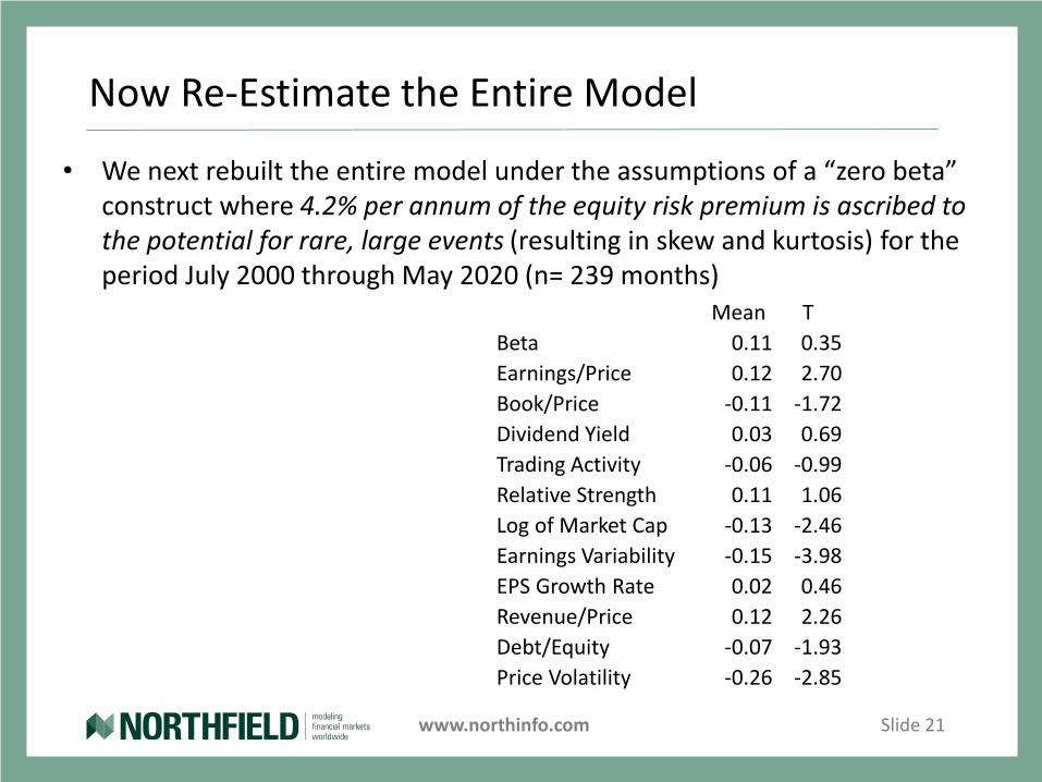
Now Re-Estimate the Entire Model

• We next rebuilt the entire model under the assumptions of a “zero beta” construct where 4.2% per annum of the equity risk premium is ascribed to the potential for rare, large events (resulting in skew and kurtosis) for the period July 2000 through May 2020 (n= 239 months)

Mean T

Beta 0.11 0.35

Earnings/Price 0.12 2.70

Book/Price -0.11 -1.72

Dividend Yield 0.03 0.69

Trading Activity -0.06 -0.99

Relative Strength 0.11 1.06

Log of Market Cap -0.13 -2.46

Earnings Variability -0.15 -3.98

EPS Growth Rate 0.02 0.46

Revenue/Price 0.12 2.26

Debt/Equity -0.07 -1.93

Price Volatility -0.26 -2.85


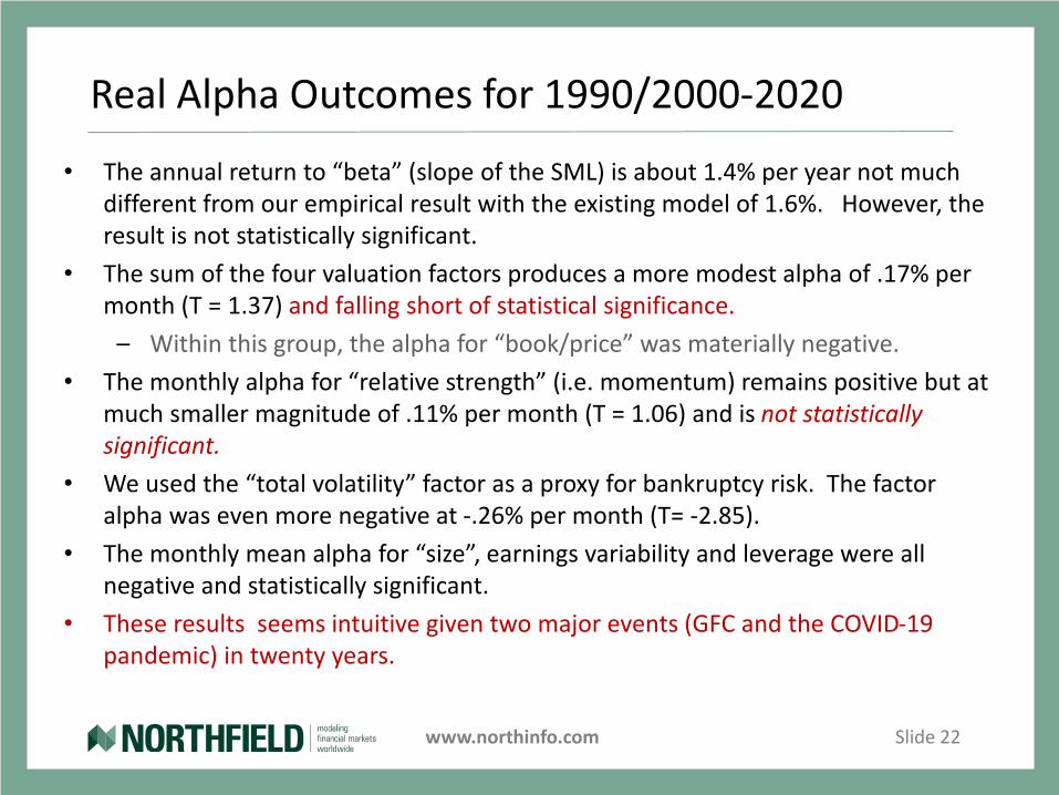
Real Alpha Outcomes for 1990/2000-2020

• The annual return to “beta” (slope of the SML) is about 1.4% per year not much different from our empirical result with the existing model of 1.6%. However, the result is not statistically significant.

• The sum of the four valuation factors produces a more modest alpha of .17% per month (T = 1.37) and falling short of statistical significance.

– Within this group, the alpha for “book/price” was materially negative.

• The monthly alpha for “relative strength” (i.e. momentum) remains positive but at much smaller magnitude of .11% per month (T = 1.06) and is not statistically significant.

• We used the “total volatility” factor as a proxy for bankruptcy risk. The factor alpha was even more negative at -.26% per month (T= -2.85).

• The monthly mean alpha for “size”, earnings variability and leverage were all negative and statistically significant.

• These results seems intuitive given two major events (GFC and the COVID-19 pandemic) in twenty years.


Factor Outcomes by Decade: 1990s

Traditional CAPM Extended CAPM

1990-1999 Mean StDev T Mean StDev T

Beta 0.95 4.14 2.51 0.53 4.78 1.22

Earnings/Price 0.06 0.59 1.20 0.09 0.81 1.16

Book/Price 0.17 0.72 2.55 0.04 0.83 0.59

Dividend Yield 0.21 0.89 2.58 0.16 0.99 1.78

Trading Activity 0.08 1.66 0.54 0.09 0.81 1.27

Relative Strength 1.13 2.07 5.97 -0.22 1.86 -1.30

Log of Market Cap 0.00 0.87 0.02 -0.37 4.60 -0.87

Earnings Variability 0.02 0.53 0.35 -0.03 0.56 -0.62

EPS Growth Rate 0.07 0.57 1.29 0.06 1.44 0.43

Revenue/Price 0.09 0.86 1.15 -0.05 0.54 -1.12

Debt/Equity -0.06 0.78 -0.84 0.64 2.77 2.53

Price Volatility 0.03 1.06 0.32 -0.03 0.89 -0.40


Factor Outcomes By Decade: 2000s


2000-2009 Mean Stdev T Mean StDev T

Beta 0.16 5.50 0.31 -0.08 5.56 -0.16

Earnings/Price 0.31 0.83 4.09 0.33 0.77 4.63

Book/Price -0.05 1.10 -0.47 0.02 1.01 0.24

Dividend Yield 0.15 0.70 2.31 0.11 0.70 1.75

Trading Activity -0.19 1.03 -1.99 -0.16 1.02 -1.68

Relative Strength 0.06 1.89 0.33 0.00 1.88 -0.03

Log of Market Cap -0.28 0.93 -3.24 -0.23 1.06 -2.33

Earnings Variability -0.24 0.73 -3.58 -0.24 0.74 -3.55

EPS Growth Rate -0.06 0.78 -0.81 -0.05 0.78 -0.64

Revenue/Price 0.16 1.06 1.67 0.17 1.03 1.80

Debt/Equity -0.07 0.69 -1.16 -0.05 0.63 -0.90

Price Volatility -0.32 1.86 -1.90 -0.29 1.55 -2.04


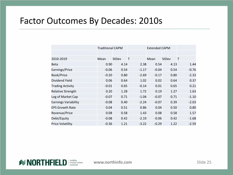
Factor Outcomes By Decades: 2010s


2010-2019 Mean StDev T Mean StDev T

Beta 0.90 4.14 2.38 0.54 4.13 1.44

Earnings/Price -0.06 0.54 -1.17 -0.04 0.54 -0.76

Book/Price -0.20 0.80 -2.69 -0.17 0.80 -2.33

Dividend Yield 0.06 0.64 1.02 0.02 0.64 0.37

Trading Activity -0.01 0.65 -0.14 0.01 0.65 0.21

Relative Strength 0.20 1.28 1.72 0.19 1.27 1.63

Log of Market Cap -0.07 0.71 -1.04 -0.07 0.71 -1.10

Earnings Variability -0.08 0.40 -2.24 -0.07 0.39 -2.03

EPS Growth Rate 0.04 0.51 0.86 0.04 0.50 0.80

Revenue/Price 0.08 0.58 1.43 0.08 0.58 1.57

Debt/Equity -0.08 0.42 -2.19 -0.06 0.42 -1.68

Price Volatility -0.36 1.21 -3.22 -0.29 1.22 -2.59


Conclusions

• Our results show that a more nuanced approach to asset pricing yields highly intuitive results.

• A large part of the equity risk premium is associated with rare but extreme events.

• A smaller part of the equity risk premium is associated with the classic CAPM view of beta as the relevant risk measure for asset pricing.

• The CAPM view that idiosyncratic risk should carry no return is refuted. We expect and find a negative return arising from bankruptcy risk at the firm level and contributing to co-skewness at the market level.

• “Smart beta” strategies that are predicated on historical excess returns alone without the context of how risks influence asset pricing are ill advised