HW1 Beta(p;4,10),Beta(p;9,15), Beta(6,6) likelihood Beta(p;1,1)

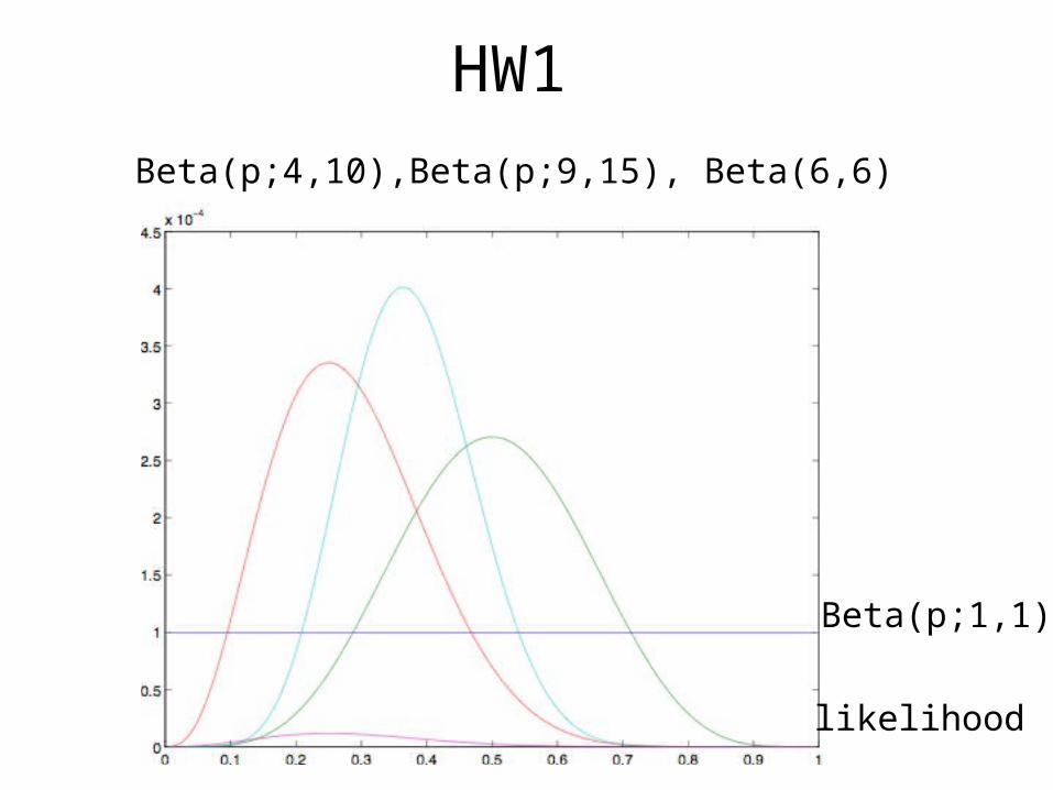
HW1

Beta(p;4,10),Beta(p;9,15), Beta(6,6)

likelihood

Beta(p;1,1)

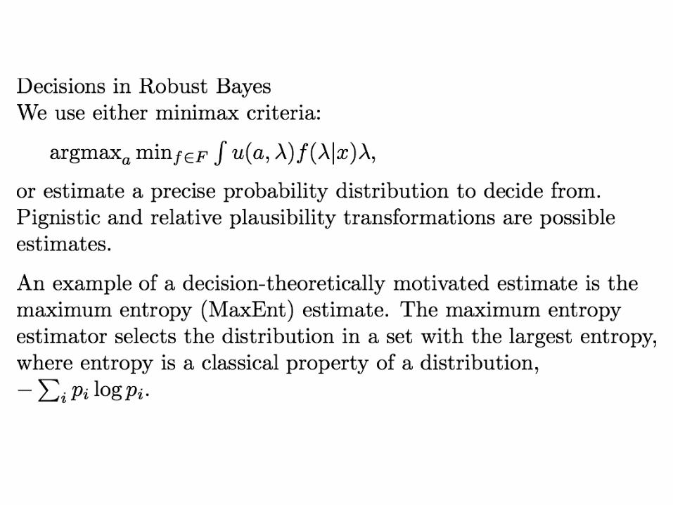
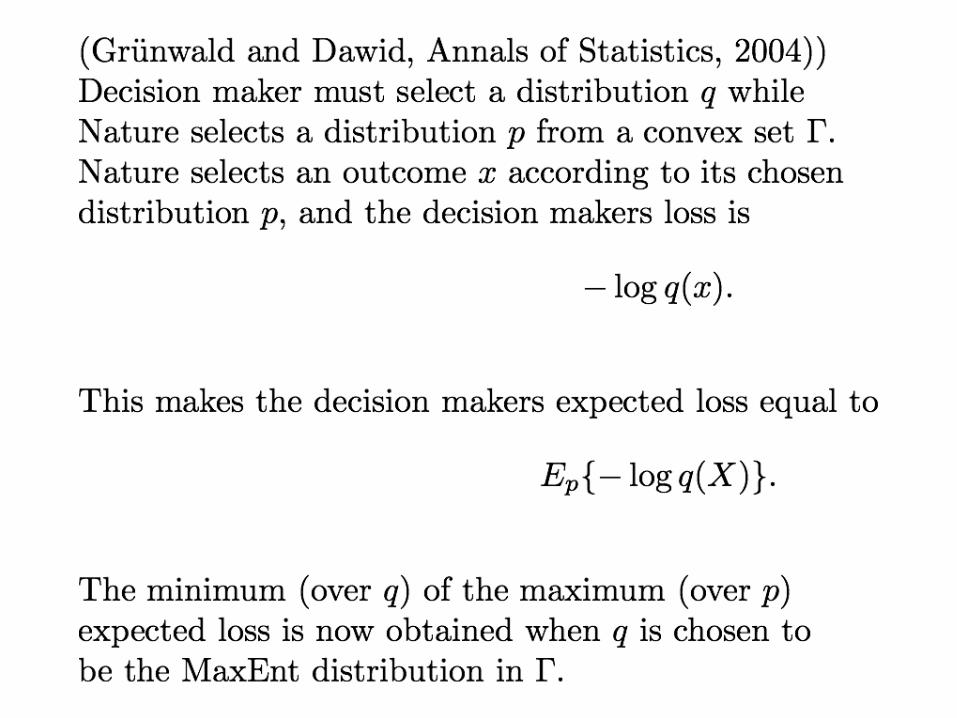
FDR, Evidence Theory, Robustness

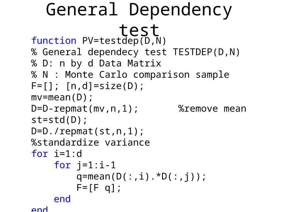
function PV=testdep(D,N)% General dependecy test TESTDEP(D,N)% D: n by d Data Matrix% N : Monte Carlo comparison sampleF=[]; [n,d]=size(D);mv=mean(D);D=D-repmat(mv,n,1); %remove meanst=std(D);D=D./repmat(st,n,1); %standardize variancefor i=1:d for j=1:i-1 q=mean(D(:,i).*D(:,j)); F=[F q]; endend

General Dependency test

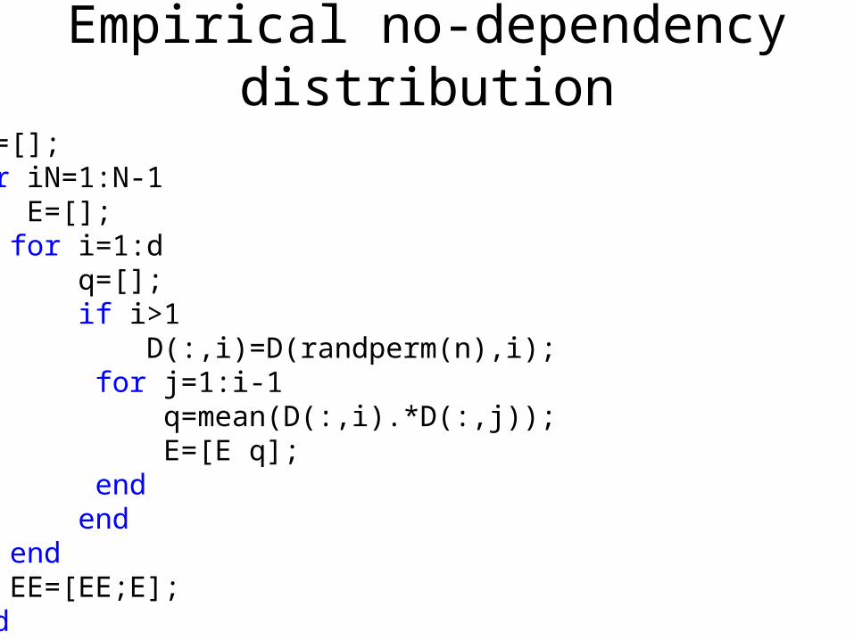
EE=[];for iN=1:N-1 E=[]; for i=1:d q=[]; if i>1 D(:,i)=D(randperm(n),i); for j=1:i-1 q=mean(D(:,i).*D(:,j)); E=[E q]; end end end EE=[EE;E];end

Empirical no-dependency distribution

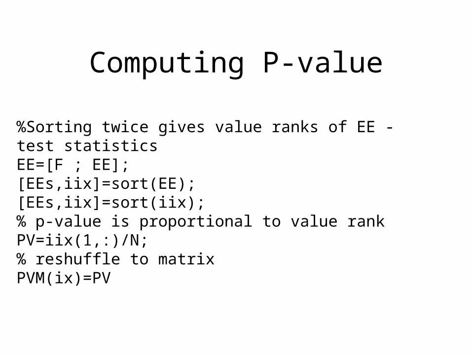
%Sorting twice gives value ranks of EE - test statisticsEE=[F ; EE];[EEs,iix]=sort(EE);[EEs,iix]=sort(iix);% p-value is proportional to value rankPV=iix(1,:)/N;% reshuffle to matrixPVM(ix)=PV

Computing P-value

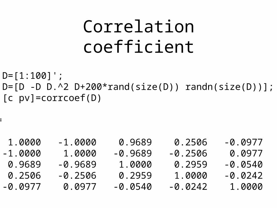
Correlation coefficient

>> D=[1:100]';>> D=[D -D D.^2 D+200*rand(size(D)) randn(size(D))];>> [c pv]=corrcoef(D)

c =

1.0000 -1.0000 0.9689 0.2506 -0.0977 -1.0000 1.0000 -0.9689 -0.2506 0.0977 0.9689 -0.9689 1.0000 0.2959 -0.0540 0.2506 -0.2506 0.2959 1.0000 -0.0242 -0.0977 0.0977 -0.0540 -0.0242 1.0000

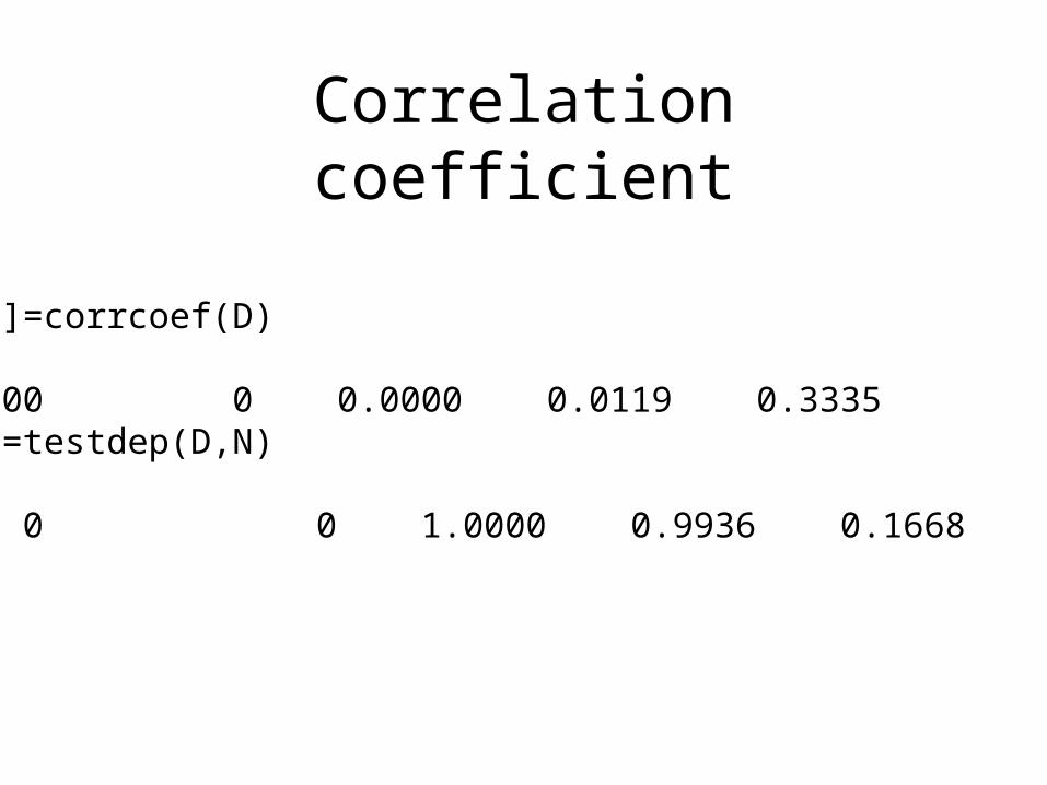
Correlation coefficient

>> [c pv]=corrcoef(D)pv = 1.0000 0 0.0000 0.0119 0.3335 >> [,pv]=testdep(D,N)pv = 0 0 1.0000 0.9936 0.1668>>

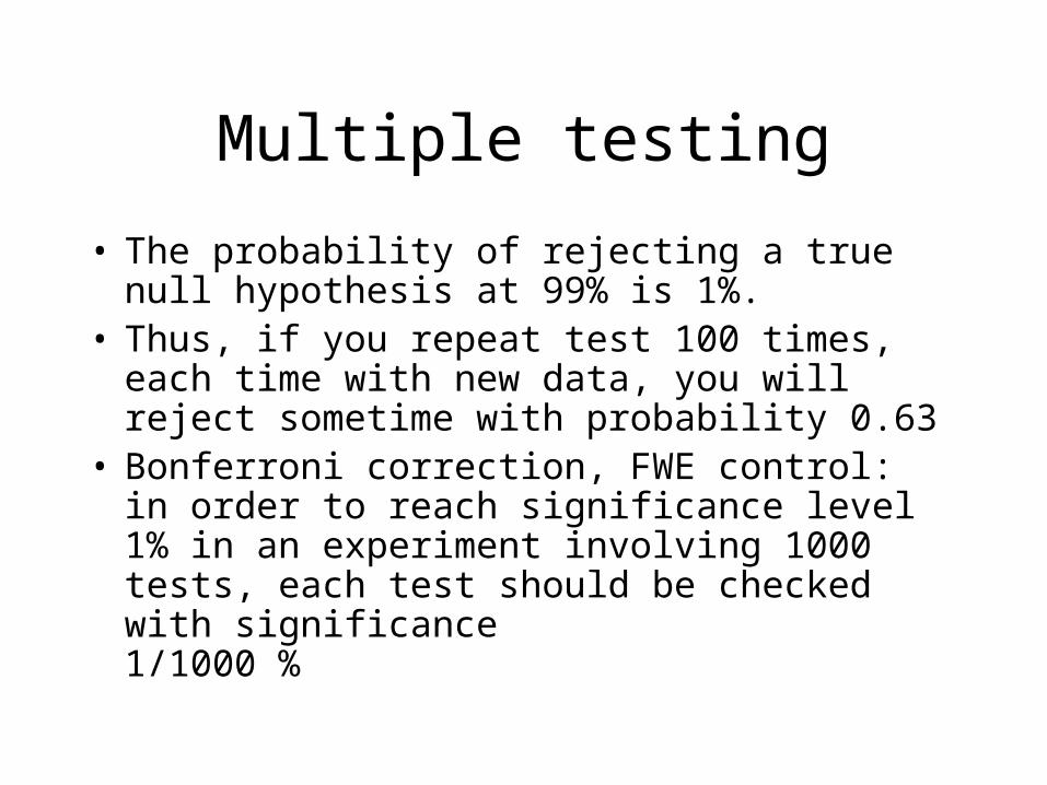
Multiple testing

• The probability of rejecting a true null hypothesis at 99% is 1%.

• Thus, if you repeat test 100 times, each time with new data, you will reject sometime with probability 0.63

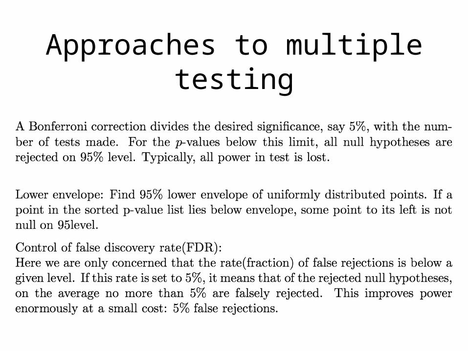
• Bonferroni correction, FWE control:in order to reach significance level 1% in an experiment involving 1000 tests, each test should be checked with significance 1/1000 %

Multiple testing

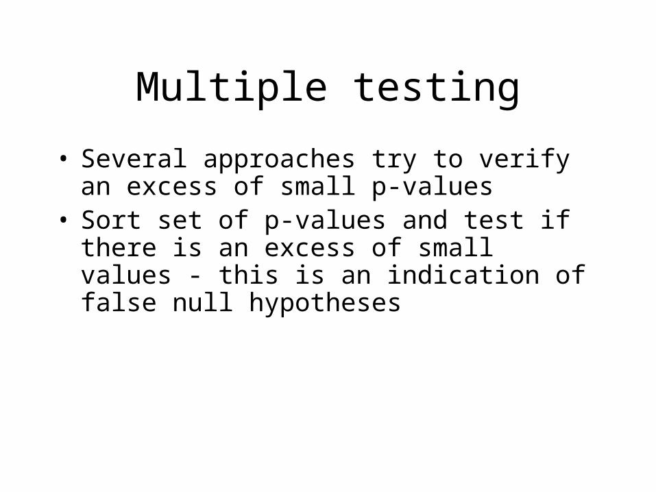
• Several approaches try to verify an excess of small p-values

• Sort set of p-values and test if there is an excess of small values - this is an indication of false null hypotheses

Approaches to multiple testing

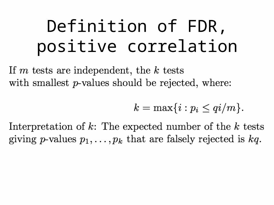
Definition of FDR, positive correlation

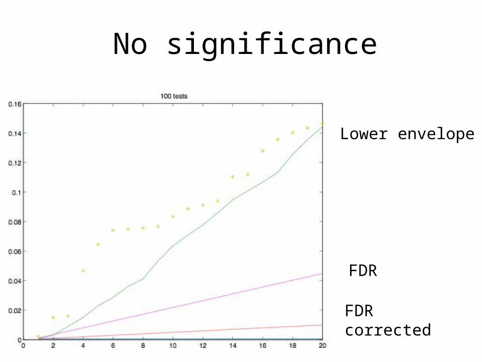
No significance

Lower envelope

FDR

FDR corrected

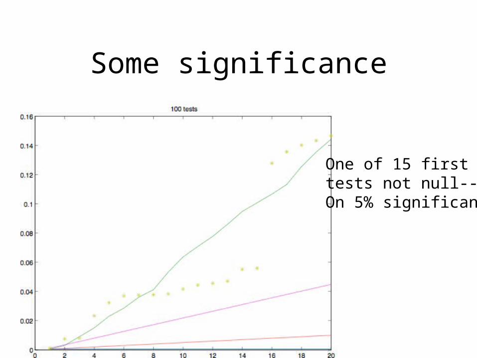
Some significance

One of 15 first tests not null--On 5% significanc

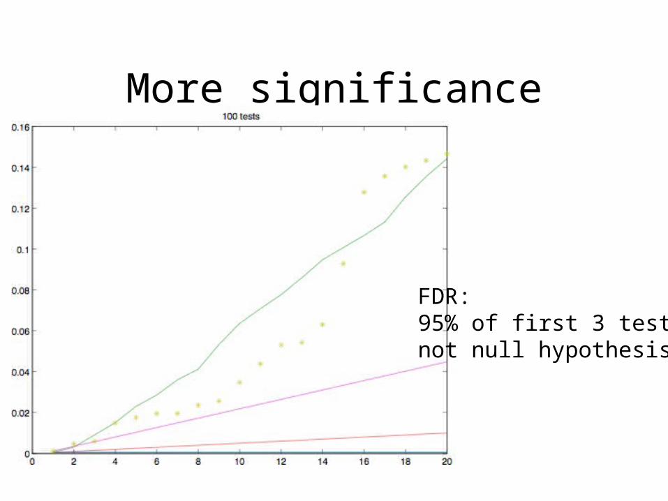
More significance

FDR:95% of first 3 tests not null hypothesis

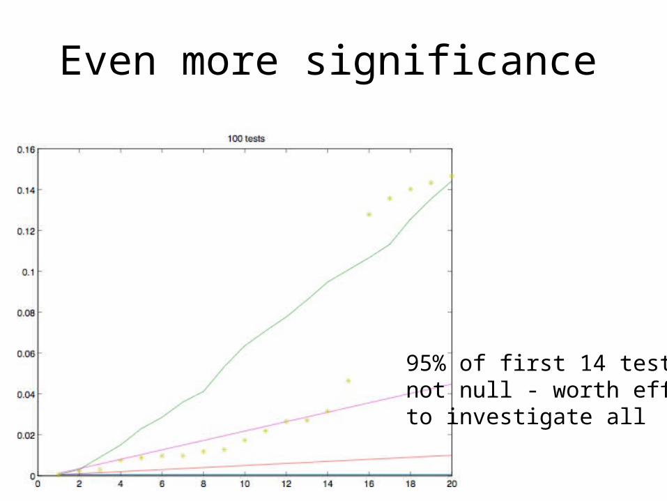
Even more significance

95% of first 14 testsnot null - worth effortto investigate all

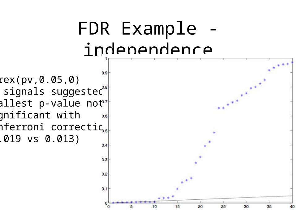
FDR Example - independence

Fdrex(pv,0.05,0)10 signals suggested.Smallest p-value notsignificant with Bonferroni correction (0.019 vs 0.013)

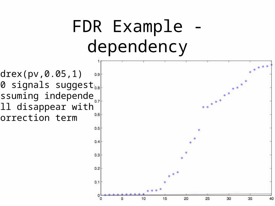
FDR Example - dependency

Fdrex(pv,0.05,1)10 signals suggestedassuming independenceall disappear with correction term

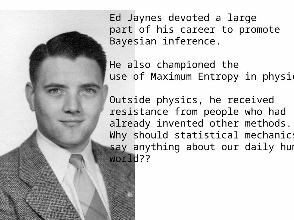
Ed Jaynes devoted a large part of his career to promoteBayesian inference.

He also championed theuse of Maximum Entropy in physics

Outside physics, he received resistance from people who hadalready invented other methods.Why should statistical mechanics say anything about our daily human world??

Generalisation of Bayes/Kalman:

What if: • You have no prior?• Likelihood infeasible to compute (imprecision)?• Parameter space vague, i.e., not the same for

all likelihoods? (Fuzziness, vagueness)?• Parameter space has complex structure

(a simple structure is e.g., a Cartesian product of reals, R, and some finite sets)?

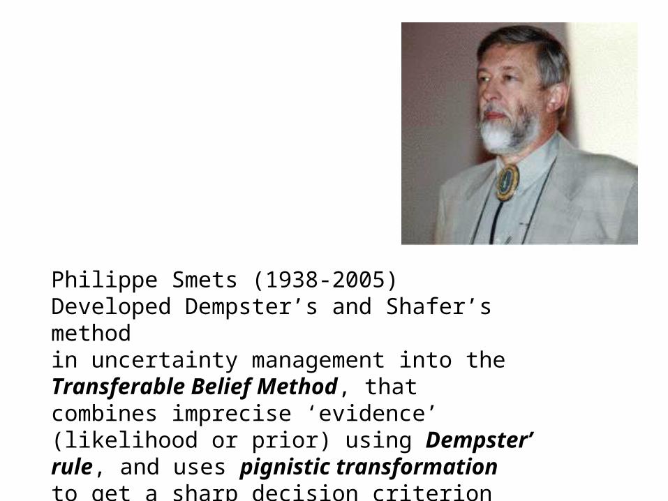
Philippe Smets (1938-2005)Developed Dempster’s and Shafer’s method in uncertainty management into the Transferable Belief Method, that combines imprecise ‘evidence’ (likelihood or prior) using Dempster’ rule, and uses pignistic transformation to get a sharp decision criterion

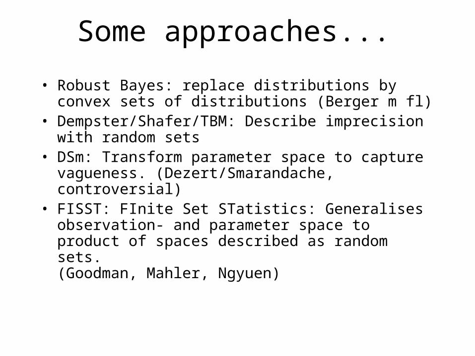
Some approaches...

• Robust Bayes: replace distributions by convex sets of distributions (Berger m fl)

• Dempster/Shafer/TBM: Describe imprecision with random sets

• DSm: Transform parameter space to capture vagueness. (Dezert/Smarandache, controversial)

• FISST: FInite Set STatistics: Generalisesobservation- and parameter space to product of spaces described as random sets.(Goodman, Mahler, Ngyuen)

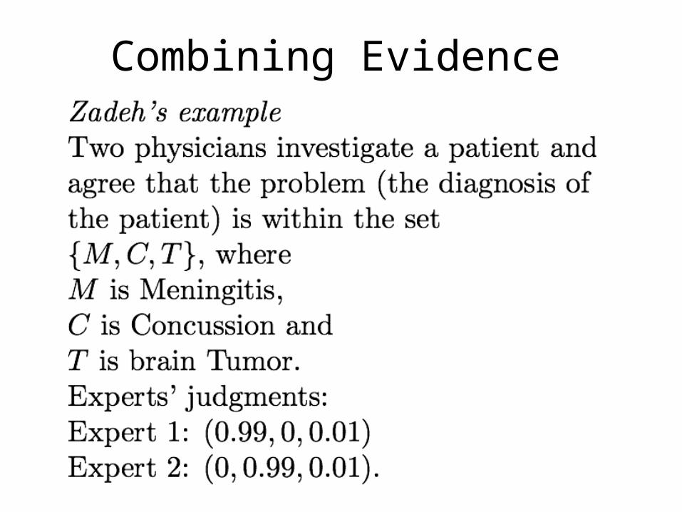
Combining Evidence

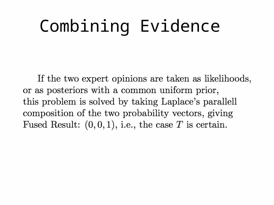
Combining Evidence

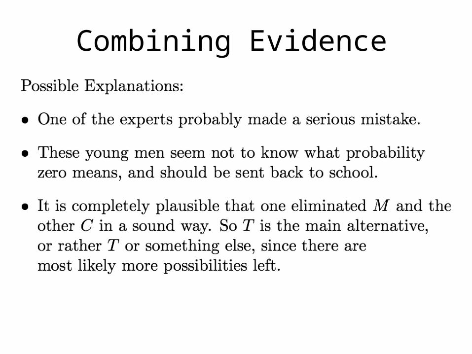
Combining Evidence

QuickTime™ and aTIFF (LZW) decompressor

are needed to see this picture.

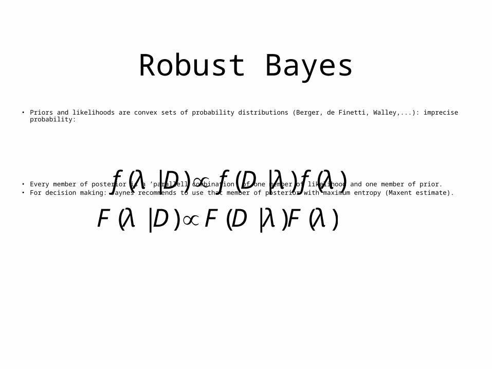
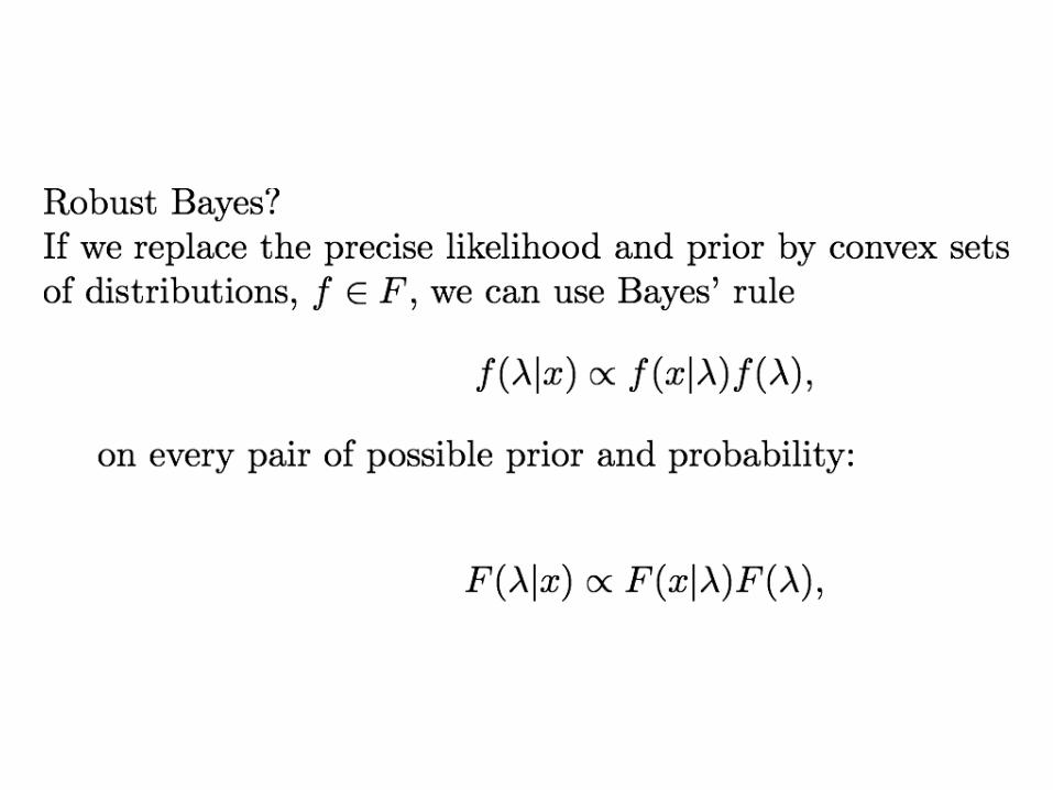
Robust Bayes• Priors and likelihoods are convex sets of probability distributions (Berger, de Finetti, Walley,...): imprecise probability:

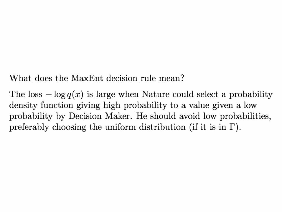
• Every member of posterior is a ’parallell combination’ of one member of likelihood and one member of prior.• For decision making: Jaynes recommends to use that member of posterior with maximum entropy (Maxent estimate).

€

f (λ |D)∝ f (D | λ ) f (λ )

€

F(λ |D)∝ F(D | λ )F(λ )

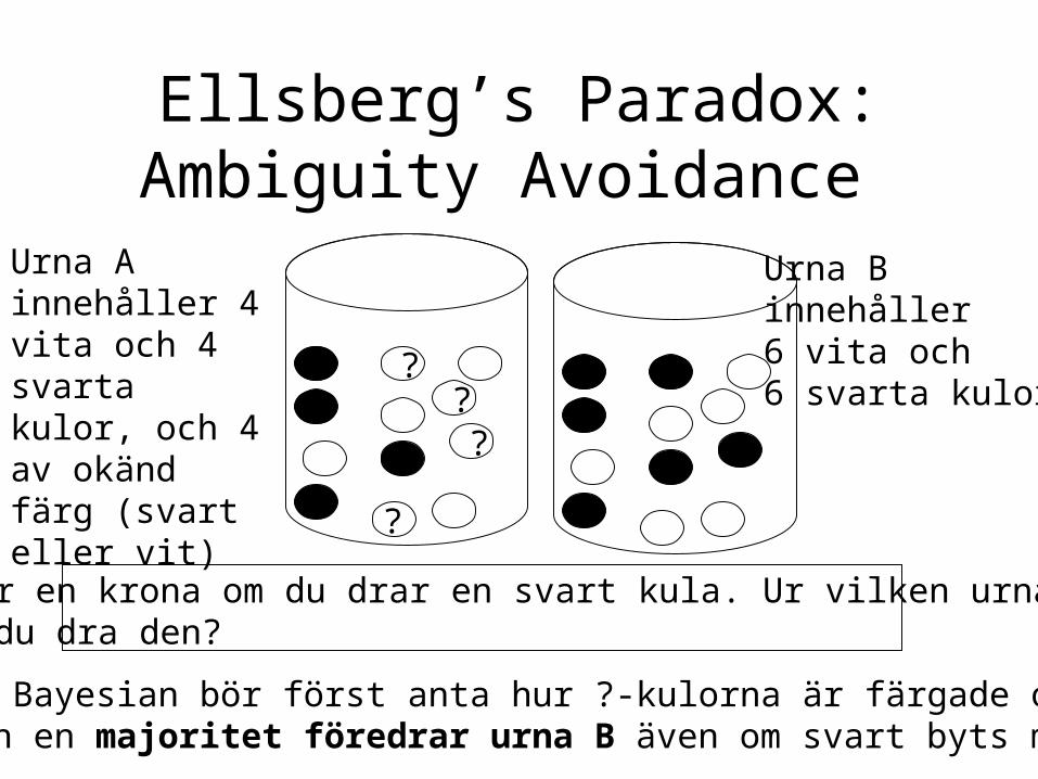
Ellsberg’s Paradox:Ambiguity Avoidance

?

?

??

Urna A innehåller 4 vita och 4 svarta kulor, och 4 av okänd färg (svart eller vit)

Urna B innehåller 6 vita och 6 svarta kulor

Du får en krona om du drar en svart kula. Ur vilken urnavill du dra den?

En precis Bayesian bör först anta hur ?-kulorna är färgade och sedansvara. Men en majoritet föredrar urna B även om svart byts mot vit

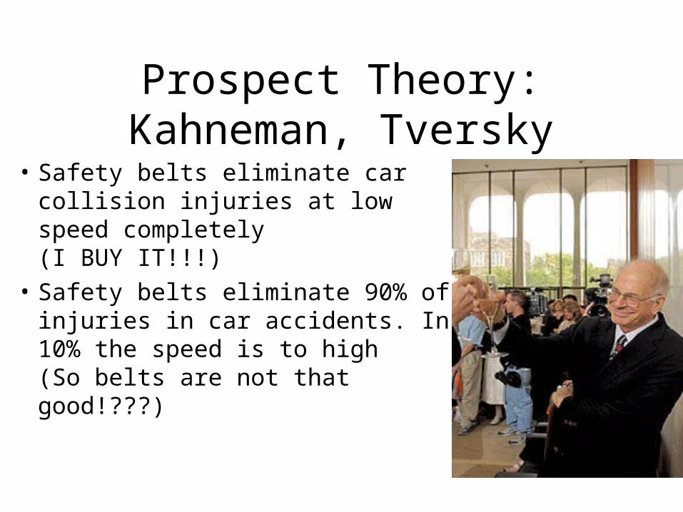
Prospect Theory: Kahneman, Tversky

• Safety belts eliminate car collision injuries at low speed completely(I BUY IT!!!)

• Safety belts eliminate 90% ofinjuries in car accidents. In 10% the speed is to high(So belts are not that good!???)

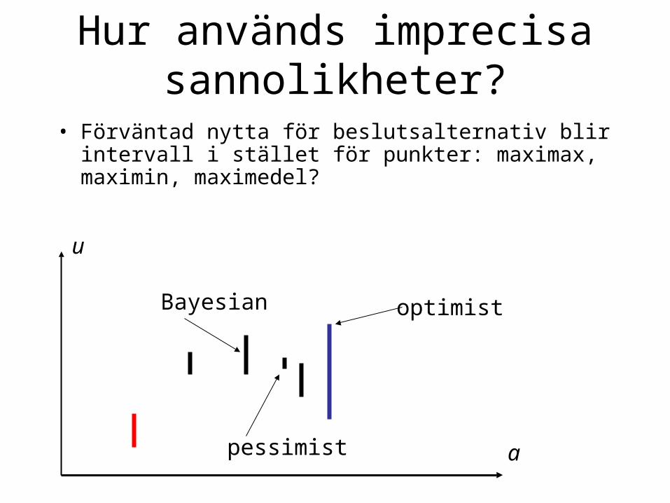
Hur används imprecisa sannolikheter?

• Förväntad nytta för beslutsalternativ blir intervall i stället för punkter: maximax, maximin, maximedel?

u

apessimist

optimistBayesian

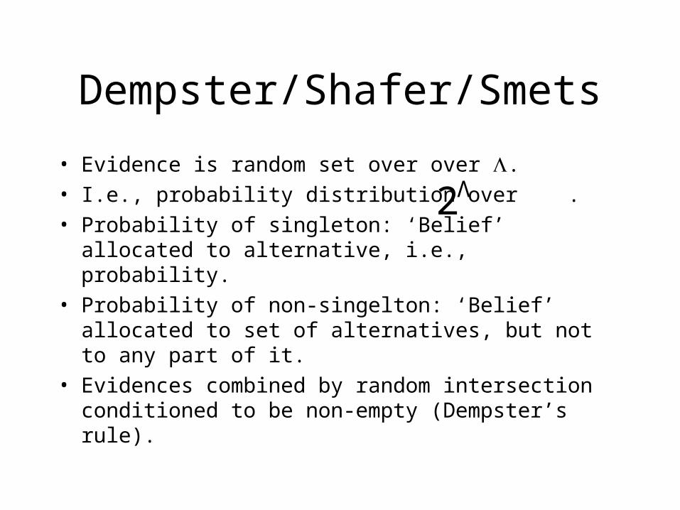
Dempster/Shafer/Smets

• Evidence is random set over over .• I.e., probability distribution over .• Probability of singleton: ‘Belief’ allocated to

alternative, i.e., probability.• Probability of non-singelton: ‘Belief’ allocated to set of

alternatives, but not to any part of it.• Evidences combined by random intersection

conditioned to be non-empty (Dempster’s rule).€

2Λ

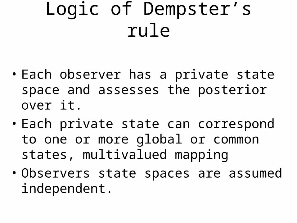
Logic of Dempster’s rule

• Each observer has a private state space and assesses the posterior over it.

• Each private state can correspond to one or more global or common states, multivalued mapping

• Observers state spaces are assumed independent.

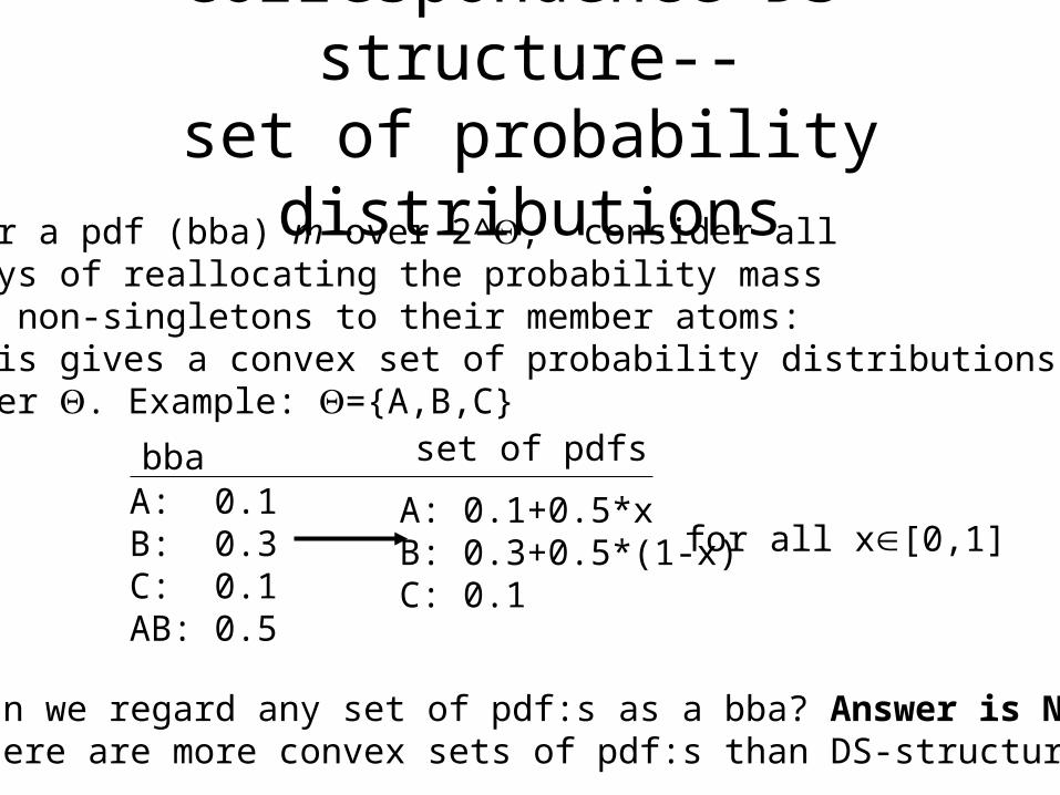
Correspondence DS-structure--set of probability distributions

For a pdf (bba) m over 2^, consider allways of reallocating the probability mass of non-singletons to their member atoms:This gives a convex set of probability distributions over . Example: ={A,B,C}

A: 0.1B: 0.3C: 0.1AB: 0.5

A: 0.1+0.5*xB: 0.3+0.5*(1-x)C: 0.1

Can we regard any set of pdf:s as a bba? Answer is NO!! There are more convex sets of pdf:s than DS-structures

for all x[0,1]

bba set of pdfs

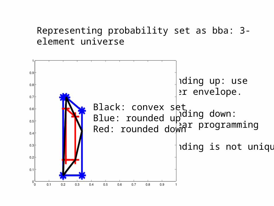
Representing probability set as bba: 3-element universe

Rounding up: uselower envelope.

Rounding down: Linear programming

Rounding is not unique!!

Black: convex setBlue: rounded upRed: rounded down

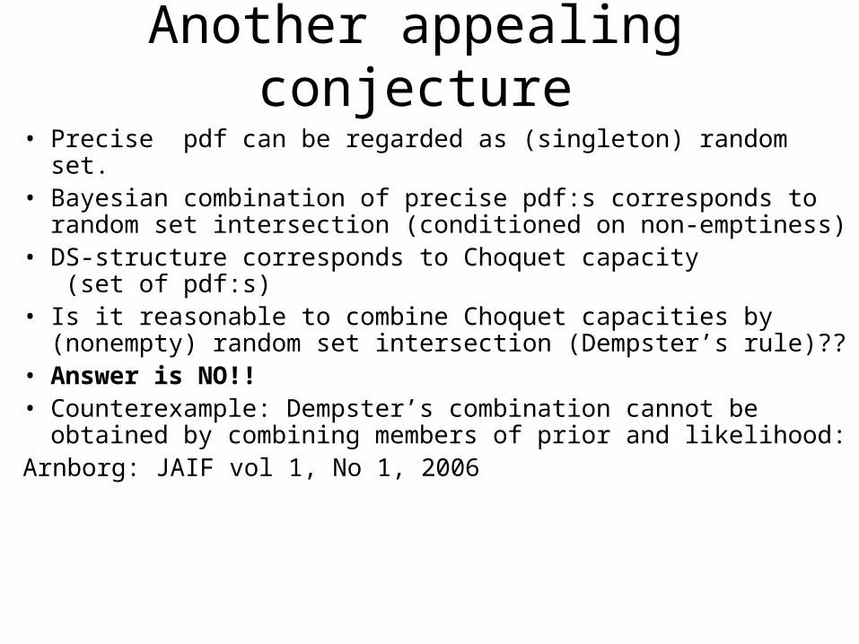
Another appealing conjecture

• Precise pdf can be regarded as (singleton) random set.• Bayesian combination of precise pdf:s corresponds to random

set intersection (conditioned on non-emptiness)• DS-structure corresponds to Choquet capacity

(set of pdf:s)• Is it reasonable to combine Choquet capacities by (nonempty)

random set intersection (Dempster’s rule)??• Answer is NO!!• Counterexample: Dempster’s combination cannot be obtained

by combining members of prior and likelihood:Arnborg: JAIF vol 1, No 1, 2006

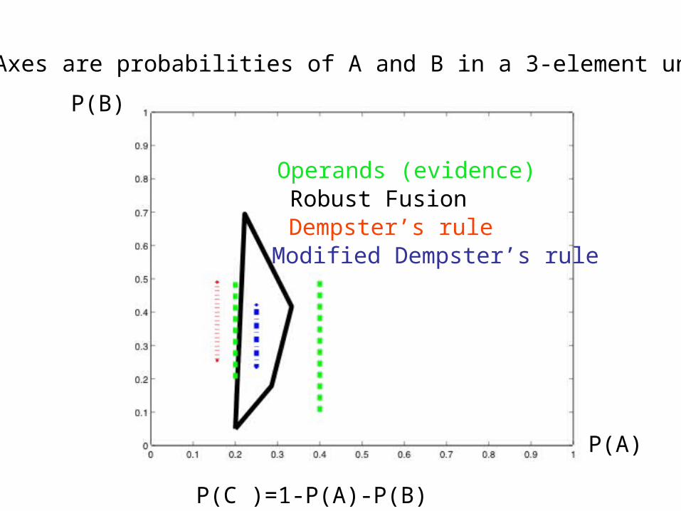
Consistency of fusion operators

DS rule

MDS rule

Rounded robust

Operands (evidence)Robust FusionDempster’s rule

Modified Dempster’s rule

Axes are probabilities of A and B in a 3-element universe

P(A)

P(B)

P(C )=1-P(A)-P(B)

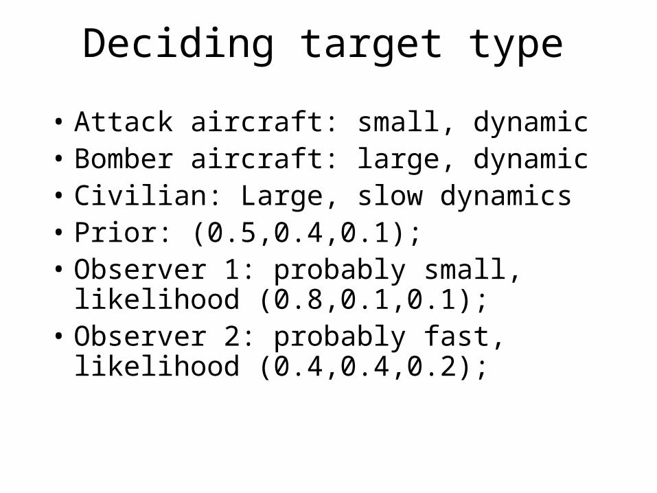
Deciding target type

• Attack aircraft: small, dynamic • Bomber aircraft: large, dynamic• Civilian: Large, slow dynamics• Prior: (0.5,0.4,0.1);• Observer 1: probably small,

likelihood (0.8,0.1,0.1);• Observer 2: probably fast,

likelihood (0.4,0.4,0.2);

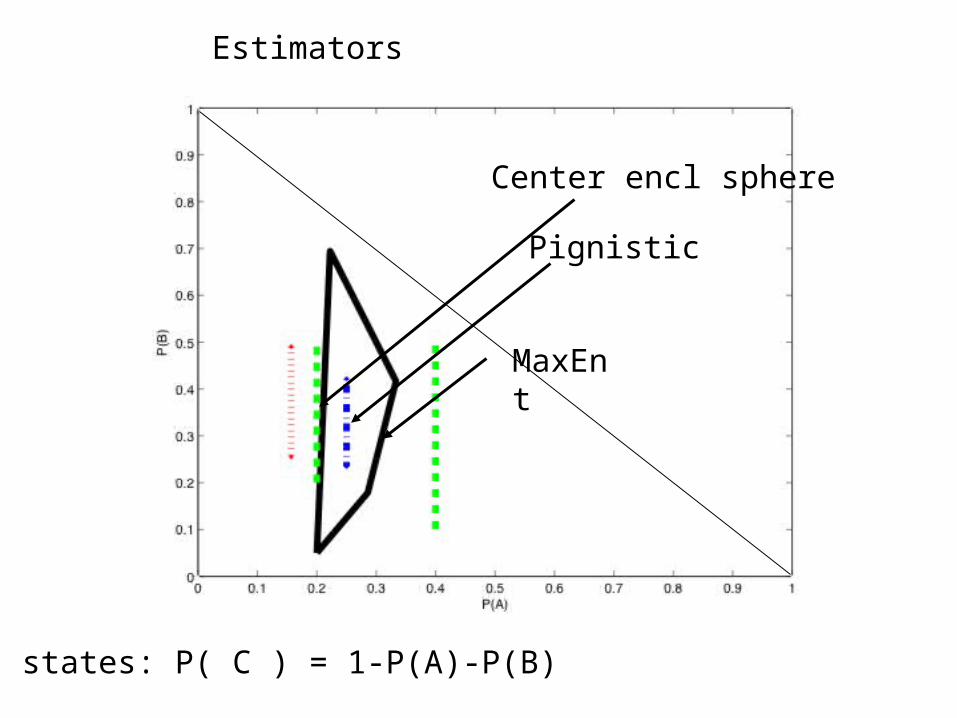
Estimators

Pignistic

MaxEnt

Center encl sphere

3 states: P( C ) = 1-P(A)-P(B)













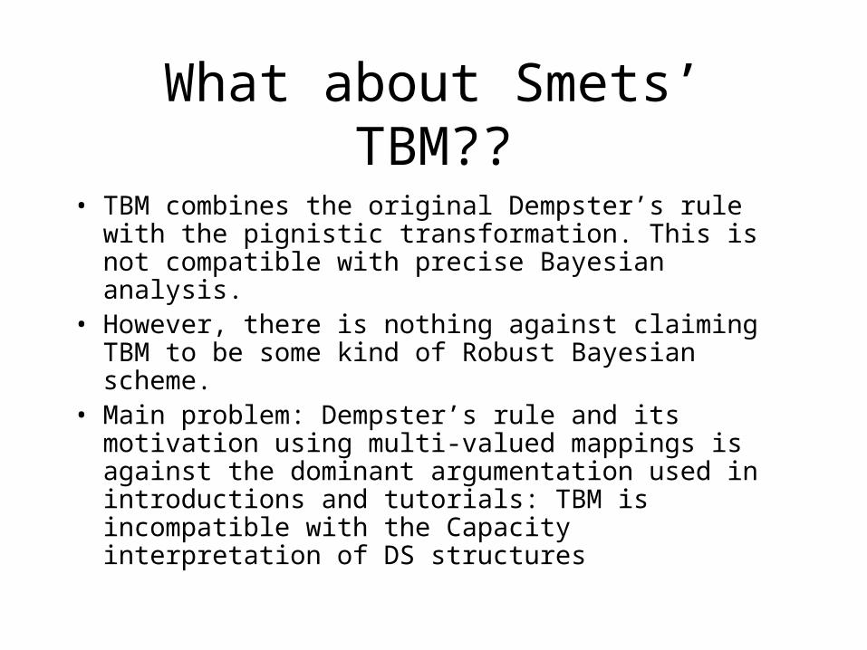
What about Smets’ TBM??

• TBM combines the original Dempster’s rule with the pignistic transformation. This is not compatible with precise Bayesian analysis.

• However, there is nothing against claiming TBM to be some kind of Robust Bayesian scheme.

• Main problem: Dempster’s rule and its motivation using multi-valued mappings is against the dominant argumentation used in introductions and tutorials: TBM is incompatible with the Capacity interpretation of DS structures

Documents

HW1 Beta(p;4,10),Beta(p;9,15), Beta(6,6) likelihood Beta(p;1,1)