Embed Size (px)
Citation preview

HOW THE ECONOMICS PROFESSION GOT IT WRONG ON BREXIT
Ken Coutts, Graham Gudgin and Jordan Buchanan
WP 493 January 2018

HOW THE ECONOMICS PROFESSION GOT IT WRONG ON BREXIT
Centre for Business Research, University of Cambridge
Working Paper No. 493
Ken Coutts CBR, University of Cambridge
Graham Gudgin CBR, University of Cambridge
Jordan Buchanan Ulster University Economic Policy Centre
January 2018

Abstract
A wide range of reports from official bodies and academics have estimated the impact of Brexit. These influenced the outcome of the Brexit referendum and remain influential in informing views on the potential long-term consequences of a range of Brexit trade arrangements. This paper builds on a previous CBR working paper (link) in examining the most influential of these reports, from HM Treasury, and the OECD. In this paper the work of the LSE’s Centre for Economic Performance is also included. Each of these reports base their analyses either on gravity models or a computable general equilibrium models. The addition in this paper a review of the link between trade and productivity, which plays an important role in these reports. We also examine three reports which take a direct approach to measuring the impact by assessing the likely prices increases across a large range of commodities due to the imposition of tariff and non-tariff barriers, and using elasticities to estimate the potential changes in the volume of trade. We find important flaws in both the application of gravity model results to a Brexit context, and in the knock-on impacts from trade to productivity. The flaws always have the result of exaggerating the negative impact of Brexit. The direct approaches involve partial rather than full equilibrium models but provide an important check on results from more complex models. However, the choice of elasticities can result in widely different results from ostensibly similar approaches. The paper starts by looking at the view, supported in the academic literature and widely repeated in the financial media, that accession to the EEC/in 1973 improved the economic growth performance of the UK. The evidence suggests that this view is incorrect. JEL Codes: C54, E24, E44, H24. Keywords: Brexit; Gravity Model; computable general equilibrium; HM Treasury; IMF; trade; macroeconomic forecasts; OECD Acknowledgements We are grateful for insights gained in discussion with Adam Slater of Oxford Economics. He is not responsible for the views expressed in this paper. We are also grateful to Rachel Wagstaff of the Centre for Business Research for considerable help in the final preparation of this paper. Further information about the Centre for Business Research can be found at: www.cbr.cam.ac.uk

1
1. Introduction Economic Forecasters in the UK have a poor record over the last decade. The failure to foresee the 2008 economic crisis has become infamous, even involving the Queen’s famous question: ‘Why did nobody notice it?’ That failure showed up how little work had been done on understanding the importance of credit markets in the UK. One aspect of this was the strange lack of a banking sector in the Bank of England model, a lacuna now being rectified. The failure to predict the crisis was followed by a large over-estimate of the speed of recovery of the UK from the 2009 recession. The tendency of the Office for Budget Responsibility to over-estimate the speed of recovery (see chart 1 below) is now recognised by the OBR itself. The OBR proposes to drop its assumption that growth in UK productivity will return to a pre-recession norm. However, the OBR will continue to base its forecasts on assumptions for productivity and population rather than attempting to forecast these things econometrically. The common tendency to describe OBR projections as forecasts rather than assumptions has compounded the importance of its over-optimism. The term ‘productivity puzzle’ sums up the profession’s difficulties in understanding the slow growth of productivity in the UK, and the related lack of growth in real wages.

2
In light of these shortcomings it might have been expected that the profession would take extra care to make its assessment of the potential impact of Brexit as fair and accurate as possible. A further failure would add substantially to the questioning of the underlying soundness of economic theory and practice related to forecasting. We argue in this paper that this did not happen and that much of the economic assessment of the impact of Brexit has been flawed, leading to a conclusion that the profession does indeed need to reassess its methods. This paper begins by questioning the view common in academic and media publications that UK membership of the EEC/EU has been beneficial for growth in per capita GDP. This is followed by a brief description of the methods used by forecasters to generate the short-term Brexit forecasts, now known to be overly pessimistic. We then briefly summarise our previous work on the use of gravity models by H M Treasury and others in assessing the amount of trade likely to be lost due to Brexit. This is followed by a review of the influential assessments of the impact of Brexit by the London School of Economics’ Centre for Economic Performance (CEP) which relies mostly on a general equilibrium approach. Then, we examine the basis for the widespread claim that any loss of trade will be accompanied by a knock-on impact on productivity. This relationship between trade and productivity commonly accounts for around half of the overall negative impact of Brexit, yet it is only lightly questioned. Finally, we assess a small number of direct, partial equilibrium estimates of the impact of Brexit on trade, plus two reports which have very recently returned to the issue of the long-term impact. Our conclusion is that most estimates of the impact of Brexit in the UK, both short-term and long-term, have exaggerated the degree of potential damage to the UK economy. We stress at this point that this is not a politically-driven exercise. Most of the four-person team behind the research for this and our other papers voted ‘Remain’ in the 2016 referendum and would do so again if given the chance. Our purpose is rather to establish a sound basis for the ongoing debate on the likely potential economic impact of Brexit, and more generally to question the quality of economic analysis in dealing with major, macro-economic policy issue like Brexit.

3
2. Did EEC/EU Membership Accelerate Economic Growth in the UK? The Brexit debate has been distorted by several myths. One of the most persistent and widely repeated is that the economic performance of the UK improved after joining the EU, (or EEC as it then was) in 1973. This claim was made by the OECD1 and was regularly stated in the media during the Brexit referendum campaign. In the academic literature the claim is most commonly associated with Professor Nick Crafts who concludes:
Overall, the evidence summarized in this section2 suggests that the timing of accession to the EU for the UK compared with France and West Germany may have played a significant part in the improvement in the UK’s relative growth performance after 1973. If the UK had stayed outside the EU, it seems very likely that growth of real GDP per person would have continued to lag behind French and German rates. (Crafts, 2016: 7)3
What neither Crafts (2016) nor Broadberry and Crafts (2010) stress is that there was no improvement in UK growth in per capita after 1973 when compared with previous decades (chart 2). Indeed, GDP per head clearly grew more slowly after accession than it had in pre accession decades. Chart 2 GDP per head Before and After Accession to the EEC/EU in 1973
Chart 2 uses ONS data from the UK National Accounts, but the conclusion is the same using Conference Board data at purchasing power parity (PPP). In this latter case the slowdown was from 2.4% per annum from 1950-1973, to 2.0% per annum for 1973-2007.This slowdown is of course greater if the period is
05
1015202530354045
1950
1953
1956
1959
1962
1965
1968
1971
1974
1977
1980
1983
1986
1989
1992
1995
1998
2001
2004
2007
2010
2013
2016
GDP per head (£000 ONS 2013 prices)
GDP per Head 2.75% pa Trend

4
extended to include the post-banking-crisis years. The slowdown is also similar if we take account of the transition period to full UK alignment with the EU tariff regime up to 1978. The claim that membership of the EU was beneficial in terms of UK GDP per head comes instead from a comparison with the original six EEC members, the EU6 (Chart 3). Over the period 1950-1973, per capita GDP in the EU6 grew at an unprecedentedly rapid average rate of 4.6% per annum measured using PPP data. This was almost twice as fast as the UK’s sedate 2.4% per annum. The UK’s growth rate was reasonably rapid by its own historical standards and was sufficient to maintain full employment through most of the period. Chart 3 Annual % change in per capita GDP. Difference between UK and EU6
Perhaps ironically, the period 1950-1973 in the UK is often termed the ‘golden age’, even by economists who argue that joining the EU was beneficial for UK economic growth. Even so, the view at the time was that the UK could grow significantly more rapidly by joining the fast-growing EEC. Another irony was that growth in the EU6 economies slowed down very soon after UK accession to the EEC. From 1979 to 2007 growth in per capita GDP in the EU6 was only 1.6% per annum, well under half of the pre-1973 rate. Per capita GDP in the EU6 in 2015 was at the same level as in 2007 although growth has picked up since then. Those who claim a UK economic benefit from EU membership argue that the UK’s economic growth improved relative to the EU6. Prior to accession in 1973 UK economic growth at 2.4% per annum had been 2.2 percentage points a year slower than the EU6. After accession, and up to the banking crisis starting in 2007, UK growth was 0.3 percentage points faster than the EU6. It is this improvement of 2.5 percentage points that is taken
Source of Data: Conference Board. Data is at Purchasing Power Parity. EU6 is a weighted average. The trend is a 5-year moving average

5
as the prime evidence of a gain from membership of the EU. Before joining the EU, the UK was a laggard relative to the EU6. After accession, the UK performed a little better than these economies for most of the period. We should notice however that the UK’s relative improvement was wholly due to the slowdown in the EU6. To repeat, there was no actual improvement in economic growth in the UK itself. To believe that the growth of the UK economy benefitted from EU membership, we must believe that the UK growth post-1973 would have deteriorated outside the EU as Crafts suggested. If the slowdown in EU6 growth was due to general world factors, including the six-fold increase in the real oil price between 1973 and 1980, this may be plausible. Such factors should however have also affected other major economies including the USA, Canada and Australia, but here the post-1973 slowdown was minor and much less than in the EU6. The slowdown in the EU6 has a much more obvious explanation. Rapid growth in these countries was initially due to post-war reconstruction and then due to post-war economic reforms in a context of reducing world trade barriers. In 1950, per capita GDP in the EU6 was only half that of the USA. By 1979 it was close to 90% of the US level. This meant that catch-up with the technological frontier represented by the USA was largely complete by the end of the 1970s. After that, growth could not be faster than the USA unless innovation, skills and efficiency rose above US levels, which they did not. Growth thus settled down at close to, or a little below, the US rate. Importantly, we would not expect the same slowdown for the UK which neither mirrored the EU6’s post-war catch-up with the USA, nor approached as close to the US level of per capita GDP. A better counterfactual for the UK economy is the USA. In this case, UK GDP per head has remained close to 70-75% of the US level throughout the post-war period. There is no sign that joining the EU improved UK economic growth relative to the USA. The only small improvement came after 2000 and was due to a minor slow-down in US growth. We can conclude that there is no evidence that joining the EU improved the rate of economic growth in the UK. Growth in the UK, as elsewhere, is constrained by technology, skills and investment. None of these has been better than the USA and hence the USA experience puts a ceiling on potential long-term growth in the UK, as it does in the EU6. The UK joined the EEC just as the EU6 catch-up ended. The UK thus joined on a false prospectus that accession would accelerate growth. It is also a fact that the previously slow growing Commonwealth markets actually expanded faster than the EU over the long period since 1973.

6
Chart 4 Per capita GDP in the UK and EU6. (USA=100)
Source of data: Conference Board. Total Economy dataset
It may be argued that even though economic growth in the UK has kept pace with the USA, growth would have been slower outside the EEC/EU. Crafts reviews the literature suggesting that openness to trade and greater FDI generally promote higher levels of per capita GDP. However, the general reduction in trade barriers under the GATT and WTO rounds, plus the liberalisation measures introduced by the Thatcher governments from 1979, were powerful influences that were in many ways independent of EU membership. Clarke et al (2017) attempt to assess the economic impact of the UK joining the EEC/EU through econometric estimation (page 185). Their ECM equations, fitted over 1950-2014 account for annual changes in real GDP in terms of the levels of GDP, and levels and changes in capital stock, skills, exchange rate and trade openness. Their EU membership dummy variable (set at one from 1973, zero otherwise) was negative but statistically insignificant. Similar equations of our own fitted over 1960-2016 are shown in Appendix A. These include world trade, domestic credit conditions and tax rates as explanatory variables. One equation shows a negative and statistically insignificant dummy variable for EEC/EU membership even if the difficult transition years 1973-1977 are omitted. However, a slightly different, specification reverses this conclusion, but any positive impact of EU membership appears to be concentrated in the period prior to 1992. After that there is no advantage. This latter equation reflects what is obvious from charts 1 and 3, i.e. that there is little evidence of an overall improvement in growth of GDP per head. If Crafts and others are correct that zero tariffs within the EU, and the subsequent reduction in non-
50.0
55.0
60.0
65.0
70.0
75.0
80.0
85.0
90.0
95.0
1950
1953
1956
1959
1962
1965
1968
1971
1974
1977
1980
1983
1986
1989
1992
1995
1998
2001
2004
2007
2010
2013
2016
GDP per Head @ppp (USA=100)
EU6
UK

7
tariff barriers within the EU, led to greater competition and higher productivity, the evidence is that these effects were either not large or were offset by countervailing influences. We do not however put much weight on a single equation approach to explaining annual growth rates in the UK. Different choices of explanatory variables lead to changing values for the EU dummies. We can note in passing, that the Treasury’s citing of Canada as an example of the gains to productivity from joining an FTA are less than convincing. HMT cited a paper by Melitz and Trefler (2012) which shows that productivity in Canadian manufacturing rose by 14% in a few years after joining the US-Canada FTA in 1989. Part of this was due to the closure of low productivity plants and part due to rising productivity within survivors. An examination of change in per capita GDP (at PPP) in the total economy however shows an immediate fall in per capita GDP and a failure to regain Canada’s pre-1989 trend for 20 years. Canada’s per capita GDP also fell relative to the USA and remained low. What may have happened is that labour which was displaced from manufacturing through increased competition within the FTA was not re-employed at equivalent wages for decades. A review of trends on per capita GDP across a range of NAFTA and EU15 members (in the latter case joining from 1973) shows few cases in which accession was followed by faster growth. 3. Short-term Impact of the Brexit Referendum Several reports published during the referendum campaign included separate estimates for both the short-term impact of uncertainty and the long-term impact of changed trading arrangements. The short-term impacts reflected assumptions that the uncertainty surrounding Brexit would undermine the confidence of companies and consumers leading to lower consumption and investment. The estimates, made in 2016, generally refer to a period before the UK leaves the EU, but some stretch into the early years outside the EU. A summary of short-term impacts from non-government sources is shown in Table 1. The UK Government’s own estimates are shown in Table 2. The estimates vary depending on what is assumed about the nature of the likely eventual relationship sought with the EU. The largest estimates of losses of GDP stem from an expectation that the UK will leave the single market and customs union and will fall back on WTO rules. Something of a consensus emerges from these studies with an expectation that uncertainty will reduce GDP (relative to a pre-referendum baseline) by around 1% after one year, 2–4% after 2 years, 3–4% after three years and 4–6% after 5 years. The Treasury’s estimates are at the high end of this spectrum of views with a view that GDP would be reduced by between 3.5% and 6%.

8
3.1 The Treasury’s Short-term Assessment The Treasury summarized its own view in the following words, ‘The analysis shows that the economy would fall into recession with four quarters of negative growth. After two years, GDP would be around 3.6% lower…. the fall in the value of the pound would be around 12%, and unemployment would increase by around 500,000, with all regions experiencing a rise in the number of people out of work. The exchange-rate-driven increase in the price of imports would lead to a material increase in prices, with the CPI inflation rate higher by 2.3 percentage points after a year’ (our emphasis added). The Bank of England and IMF agreed that recession was possible4. The mechanism underlying the Treasury assessment is that:
• Firms and households would begin adjusting to the expected new relationship with the EU.
• Household consumption and business investment would be damaged by
uncertainty.
• Financial markets would react immediately with a 10–14% fall in the sterling exchange rate. Credit conditions would tighten and equity prices would fall, leading to a 10-18% reduction in house prices relative to the baseline.
These effects were entered into the NiGEM5 macro-economic model which then generated further effects including real wages reduced by the higher prices caused by the sterling depreciation. Lower real wages in turn further reduced consumer spending. Exports would be higher and imports lower but the overall impact would be sharply negative. Table 1 HMT Summary of Studies of Short-term Impact of Brexit on GDP
Source: H.M. Government (2016). H.M. Treasury Analysis: The Long-term Economic Impact of EU Membership and the Alternatives, April 2016. Cmnd. 9250. Box 3.D

9
Table 2 HM Treasury Estimates of the Short-term Impact of Brexit
Source: H.M. Government (2016). H. M. Treasury Analysis: The Immediate Economic Impact of Leaving the EU. May 2017 Cmnd. 9292, p. 8. Writing more than eighteen months after the referendum result, only one of the Treasury’s expectations has been clearly realized. This is the fall in the value of sterling, and the consequential rise in inflation. A 10-15% fall in the effective exchange rate matches the HMT ‘shock’ scenario, but is also close to its ‘severe shock’ scenario. No recession materialised over the 12 months following the referendum. Nor has unemployment risen. In autumn 2017, fifteen months after the referendum, unemployment has fallen to its lowest level for 33 years, and shows little sign of rising. The UK Treasury expectation that equity risk premia would rise, leading to lower equity prices, has thus proved wrong. The sterling depreciation instead led to higher UK equity prices as corporate earnings from abroad became worth more in sterling. While there was no sign of an economic slowdown in the second half of 2016, and certainly no recession, growth slowed a little in 2017. With four quarters of data now available, it looks likely that growth in GDP in 2017 will be 1.8%. Growth in consumption has fallen since 2016, but business investment has experienced healthy growth in 2017 in contrast to the decline in 2016. There are few signs of actual decline. Estimates of the impact of Brexit per se have been calculated using our UKMOD econometric model of the UK economy. Even in the absence of Brexit, economic growth was expected to slow in 2017 due to continuing government austerity and constrained growth of mortgage credit. Uncertainty over Brexit in 2017 is calculated to have reduced consumption and company investment by 0.25% and household investment by 0.5%. These constraints are however offset by 10-15% depreciation in the sterling effective exchange rate and small relaxations in fiscal and monetary policies. Overall, our estimate is that the Brexit referendum result has made little difference growth in

10
GDP in 2017 compared with what we predict would have happened without the referendum, and is expected to do the same in 2018. Estimating the short-term impact of Brexit in 2017 depends on calculating a counter-factual forecast. Others may make different calculations, but the forecasts listed above for private sector forecasters of a 1% reduction in GDP imply that, with an outturn of 1.8% growth, GDP growth without Brexit would have been 2.8%, which is higher than any year since 2007 except for the pre-election year 2014. There were several reasons why HMT got its short-term forecasts so badly wrong.
• HMT’s transition effect was too large because the long-term losses towards which the economy was transitioning were exaggerated. This issue is described below.
• The impact of uncertainty depended ultimately on assumptions, which proved to be wrong. An index of uncertainty was constructed, with a VAR model to link uncertainty to a range of economic variables. However, there was little on which to base a judgement on how much uncertainty would be created by the referendum result. HMT made a guess, assuming a 1 to 1.5 standard deviation rise in uncertainty. Their forecasts for GDP etc. should have revealed that they were based on assumptions.
• Assumptions were also used to obtain the financial markets effects.
Increases were assumed in interest rates on loans and on equity risk premia (leading to lower equity prices). These assumptions proved wrong, at least for the twelve months following the referendum. The obvious point that a sterling depreciation would raise share prices in sterling due to a higher sterling value for firm’s foreign currency earnings was missed by HMT.
• It was assumed that short-term interest rates and government expenditure plans would remain unchanged. In the event the bank rate was lowered, and expenditure plans were raised, albeit by a small amount.
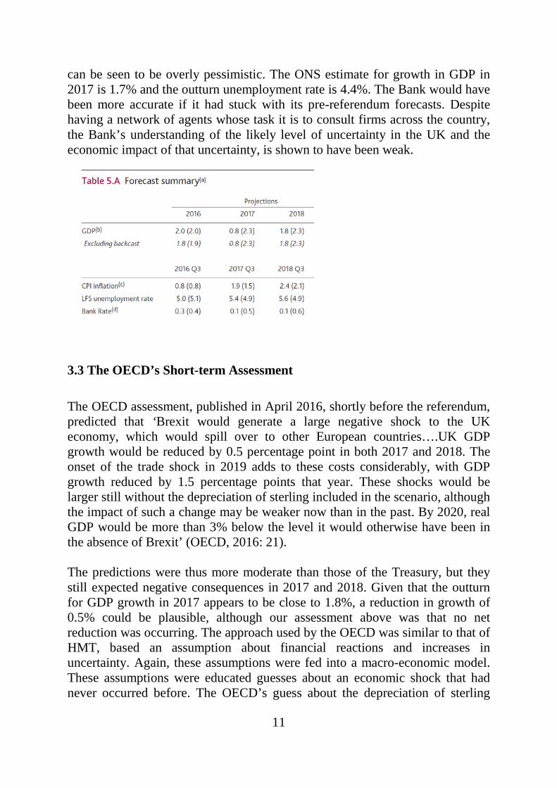
3.2 The Bank of England’s Short-term Forecasts The Bank of England published a set of economic forecasts in its August 2016 Inflation Report published two months after the Brexit Referendum result and soon after its decision to reduce the bank rate from 0.5% to 0.25%. The forecasts are reproduced below, with the pre-referendum forecasts included in parentheses. The forecasts for 2017 can now be compared with the outturns, and
11
can be seen to be overly pessimistic. The ONS estimate for growth in GDP in 2017 is 1.7% and the outturn unemployment rate is 4.4%. The Bank would have been more accurate if it had stuck with its pre-referendum forecasts. Despite having a network of agents whose task it is to consult firms across the country, the Bank’s understanding of the likely level of uncertainty in the UK and the economic impact of that uncertainty, is shown to have been weak.
3.3 The OECD’s Short-term Assessment
The OECD assessment, published in April 2016, shortly before the referendum, predicted that ‘Brexit would generate a large negative shock to the UK economy, which would spill over to other European countries….UK GDP growth would be reduced by 0.5 percentage point in both 2017 and 2018. The onset of the trade shock in 2019 adds to these costs considerably, with GDP growth reduced by 1.5 percentage points that year. These shocks would be larger still without the depreciation of sterling included in the scenario, although the impact of such a change may be weaker now than in the past. By 2020, real GDP would be more than 3% below the level it would otherwise have been in the absence of Brexit’ (OECD, 2016: 21). The predictions were thus more moderate than those of the Treasury, but they still expected negative consequences in 2017 and 2018. Given that the outturn for GDP growth in 2017 appears to be close to 1.8%, a reduction in growth of 0.5% could be plausible, although our assessment above was that no net reduction was occurring. The approach used by the OECD was similar to that of HMT, based an assumption about financial reactions and increases in uncertainty. Again, these assumptions were fed into a macro-economic model. These assumptions were educated guesses about an economic shock that had never occurred before. The OECD’s guess about the depreciation of sterling

12
was too low, and in practice the pound fell by twice the amount the OECD expected. As a result, the boost to economic growth from the depreciation has been larger than expected and has played a larger role in offsetting reductions in growth due to uncertainty. The assumption about the impact of uncertainty on consumption in 2017 seems about right. OECD assumed increases in bond spreads and equity risk premia that have not occurred by the end of 2017. They did not allow for the easing of monetary policy, and like HMT failed to foresee the boost to UK share prices in sterling. Looking slightly further ahead, the OECD envisaged an 8% loss of trade if no trade deal was in place. Again, this was more moderate than the Treasury prediction, as was the assumed knock-on impact from trade to productivity. To anticipate the discussion below, our view is that trade losses will be even smaller and that there will be no knock-on impact on productivity. Unlike HMT the OECD assume a reduction in migration of 84,000 per annum from 2019. An actual reduction of close to this magnitude has already occurred in 2016 and 2017, and this seems to be due to both the fall in sterling and a Brexit ‘chill effect’. Overall, the OECD’s assumptions were more reasonable than those of the Treasury. Now that data is available for much of 2017 we can judge that some of these were too pessimistic. Financial predictions are always difficult and in this case the OECD expected a larger negative reaction than has occurred to date. The OECD’s assumption on the impact of uncertainty on consumption seems reasonable for 2017, but the offsetting gains from depreciation were too small. The small overall prediction in 2017 is not unreasonable, but is nonetheless too large.
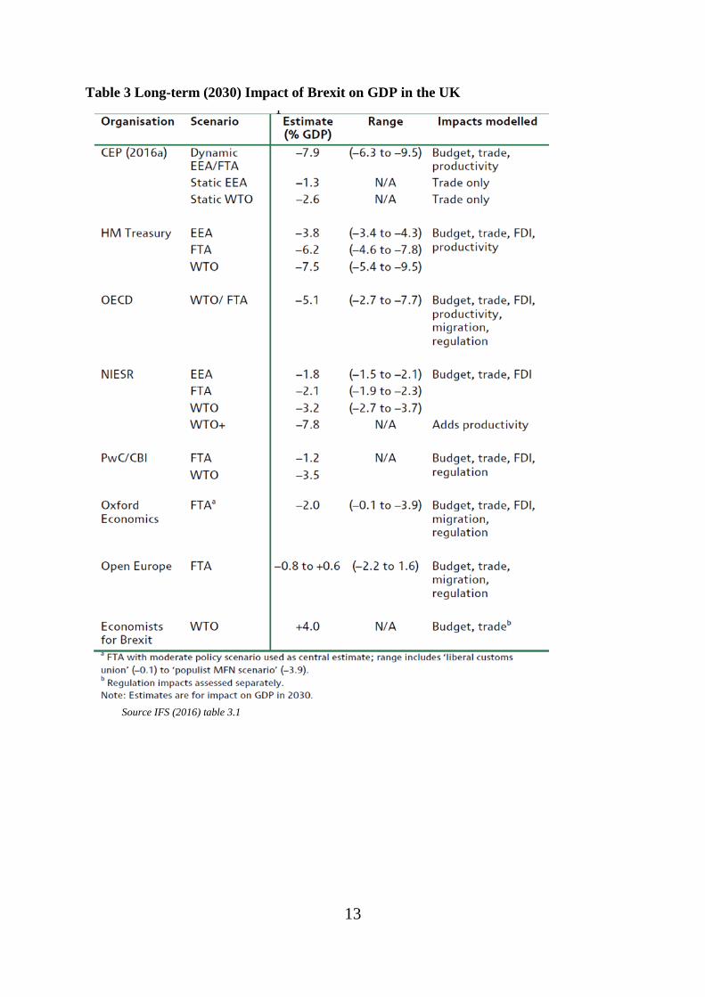
4. Long-term Impact of the Brexit Referendum Once again, a substantial number of reports were written during the referendum campaign on the long-term impact of Brexit. Some of these have been subsequently updated. A range of results was generated, nearly all of them suggesting a negative long-term impact. Most reports considered a range of potential Brexit scenarios including a free-trade agreement and no-deal on trade leading to a reliance on WTO tariffs and non-tariff barriers. A range of predictions is shown in Table 3 and chart 5. In this section we focus on the WTO scenarios as a worst case.
13
Table 3 Long-term (2030) Impact of Brexit on GDP in the UK
Source IFS (2016) table 3.1

14
Chart 5 Estimates of Long-term Impact of Brexit on UK GDP
Note: the ranges shown in this chart cover all of the possible forms of Brexit. The most negative (LHS) end of each range represents no deal on trade.
4.1 The Long-Term Forecasts of HM Treasury The Treasury approach involved using gravity models to calculate how much extra UK trade was undertaken with the EU as a result of the UK’s membership. It was then assumed that most of this additional trade would be lost to the UK on leaving the UK and adopting WTO rules. A similar exercise was undertaken for foreign direct investment (FDI). An additional knock-on impact on productivity was added to reflect a belief that productivity is positively related to trade openness and lower FDI. Finally, the results of these exercises were entered into the NiGEM macro-economic model to generate forecasts for GDP, unemployment etc. In this section we briefly repeat our previous work which replicated the Treasury’s gravity model analyses to estimate the potential trade losses from Brexit. This work reproduced the Treasury gravity model analysis for trade in goods, involving a huge data base of trade and other variables including almost a million pieces of data. As far as we know we are the only research group to have done so, and hence are the only group fully capable of identifying the key short-comings in the Treasury analysis. The productivity links are dealt with in a later section.

15
The gravity model-based methods used by the Treasury are described in HM Treasury April (2016a) and in Gudgin et al (2017a and 2017b). The approach involves analysing trade flows between around 120 countries over a 65-year period and estimating an equation relating bilateral trade to the size of the two economies in each trade pair, their distance apart and other factors such as a common language. This basic gravity equation is then used to estimate how much more trade is conducted between countries that are both members of the EU than between other trade-pairs. There are several important short-comings in the Treasury’s use of the gravity model approach to measuring the impact of EU membership on trade:
• The number of country pairs is very large, many of which are small developing nations undertaking minimal trade with the UK. The inclusion of such countries affects the underlying gravity equation and hence the size of the average deviation from the underlying equation. In technical terms the variance of trade is much higher for small countries than large countries and hence the measured errors are heteroscedastic.
• The Treasury measures the average impact of EU membership across all EU members and does not investigate whether this calculated impact is relevant to the UK alone. When we replicate the Treasury analysis we find that there is a large and significant negative residual for the UK. Indeed, the Treasury Report provides virtually no information directly about UK trade with the EU. We will return to this issue below.
• Although the Treasury does not in all cases assume that the benefits to trade of EU membership are fully reversed on leaving, in their upper (worst-case) scenario they do assume a full reversal of benefits, despite the fact that UK firms must currently be compliant with EU regulations and are likely to maintain compliance to continue trading.
The Treasury analysis contains further weaknesses
• The Treasury makes no allowance for changes in migration as a
consequence of Brexit. It thus assumes that any change in GDP is mirrored by a change in per capita GDP
• Despite predicting a depreciation of sterling in its ‘Immediate Impact’ report, the Treasury makes no allowance for a long-term lower level of the sterling exchange rate which might offset higher costs imposed by EU tariffs. If the large post-referendum depreciation in sterling proves to be permanent, this will offset much, or all, of the increases in costs due to

16
higher tariffs in most sectors. In the academic literature on trade, gravity models generate estimates of the impact of EU membership on exports which are variable but for all EU members are always positive and significant. The Treasury’s review of the gravity model literature also found a wide variety of estimates for the average impact of EU membership on trade in both goods and services. Their table A.5 is reproduced below. This shows that the gravity model technique can generate different results dependent on the data sources, periods used and other aspects of the precise methodology. Gudgin et al (2017a) apply a range of different ways of applying the gravity approach. All of these alternative estimates for the average EU effect across all member states are lower than that of the Treasury with the range of estimates still approximating to a doubling of export goods trade inside the EU. However, the most important point is that this average impact does not relate directly to UK trade. The UK is the only EU state, other than Malta, which exports more to non-EU countries than to other EU member states. UK exports of goods to the EU have usually been well below the levels predicted by these gravity model equations. Instead of the Treasury’s average impact across all 28 EU member states of around 115% extra trade, the increase in the UK alone appears to be much lower, in the range 20-25%. There is evidence that the impact on UK exports was somewhat higher than this before 2000, which accords with the evidence from time series trends showing that the share of UK exports (of goods and services) rose rapidly from accession in 1973 to 1990. Since 1990 the share first stalled and in recent years has been falling rapidly as non-EU markets have grown much faster than those within the EU and within the Eurozone. An analysis at company level finds that many British companies have been diversifying their trade away from the EU (Mayer et al., 2017).

17
HM Treasury Table A.5 External and HM Treasury estimate of EU and FTA membership effects _____________________________________________________________________________
EU Membership Effect FTA Membership EffectHM Treasury 68%/76%/85% 14%/17%/21%OECD(2015) 60% N/ABaier,Bergstrand et al (2008) 92% 58%Hufbauer and Schott(2007) 31% 27%Carrere(2006) 104% N/AEicher and Henn(2011) 37% InsignificantEicher et al(2012) 51% N/A_____________________________________________________________________________The range of impacts for the HM Treasury results is based on using a +/_1 standard error range____________________________________________________________________________
The Treasury’s estimated uplift in goods exports due to EU membership is 115%. A similar exercise for services trade gives an uplift of 24%. The weighted average for both goods and services is 76%. If fully reversed, this overall uplift of 76% gives a loss for EU trade in goods and services of 43%. This is equivalent to a loss in total trade (both EU and non-EU) of 24%. However, not all of the gains are likely to be reversed, and especially not immediately. While tariffs on goods may be imposed overnight if the UK reverts to WTO rules, these tariffs are much smaller than when the UK joined the EEC in 1973. For many non-agricultural commodities the tariffs are now very low. Even if there is new free-trade agreement, evidence suggests that many firms may prefer to pay the (low) tariffs to avoid paperwork (Keck A and Lendle A, 2012). With the UK outside the customs union, there will also be additional administrative costs but the WTO Trade Facilitation Agreement of February 2017, recently signed by the EU, will help to minimise these. Other non-tariff barriers should be initially low since UK firms are mostly already compliant with EU regulations. The Treasury takes this latter point into account in its low and medium impact projections but not for its high (no-trade deal) projection. Our estimate for the impact of no deal on UK exports is much lower. The total loss of EU exports of goods due to tariff and non-tariff barriers is 20-25%. In Gudgin et al. (2017) we did not calculate trade losses for services and implicitly accepted the Treasury estimate of a 20% loss for services, even though we had little detail on the Treasury analysis for services. We have subsequently become aware of a study of service trade (Walsh, 2006). This finds that services trade is influenced by size of economy and common language but not by distance. The growth of internet and social media usage since 2006 is likely to have strengthened this conclusion on distance. Walsh found no significant trade uplift

18
due to EU membership, although we do not know whether this conclusion applied specifically to the UK. If were to accept Walsh’s conclusion of no EU membership impact on services trade with the EU, then our estimate of the total loss of EU trade following no deal on trade would be 12%. This equates to a 5% loss of total (EU plus non-EU) trade. This is much smaller than the Treasury’s estimate of 24% for the loss of trade in the event of no deal on trade. In our view, not all of the trade gains would be lost. UK firms would face a trade weighted tariff of around 4%, but outside food, drink, clothing and vehicles the tariffs are lower at around 1-2%. If firms were to increase their prices by the amount of the tariff and face an average price elasticity of -2 on their sales, then the loss of exports might be 4-8%. Regulatory issues should initially be minor due to the existing compliance of UK firms with EU rules, although there may be regulatory divergence over time. Kee and Nicita (2017) suggest that the loss of UK goods exports might be as low as 2% since commodities facing higher tariffs tend to have low price elasticities. We havebeen unable to get a meeting with the Treasury to discuss these differences, nor were HMT willing to release any further details of their methods or equations. We do know however that there is an internal Treasury paper from 2005 which generates much smaller estimates of the impact of EU membership on intra-EU trade (HM Treasury, 2005). Importantly, this paper recognises that the impact of EU membership was much smaller for the UK than for other EU members. We had assumed that HMT’s failure to recognise this key point in their 2016 report was due to an oversight, but the existence of the 2005 Treasury paper suggests that it was more deliberate. The omission could, of course, be due to a lack of institutional memory in an organisation with high staff turnover, but it is important to note that the official responsible for the 2016 report, Treasury Chief Economist, Sir Dave Ramsden (now Deputy Governor at the Bank of England), was employed at the Treasury in 2005. 4.1.1 Foreign Direct Investment The Treasury Report’s analysis of the impact of Brexit on foreign direct investment (FDI) also uses a gravity model applied to OECD and UNCTAD data and estimated across 40 countries for the period 2000-2012. The data are financial, i.e. the value in money terms of the change in the stock of foreign-owned businesses within a country. HMT find that EU membership increases FDI flows within the EU by 35%, but there is no significant increase in FDI flows into EU members from outside the EU. The latter finding, of no increase from outside the EU is ignored by HMT. The analysis instead assumed that the

19
scale of flows from outside the EU should be the same as for intra-EU flows. If we follow the Treasury and take the estimate of a 22% mid-range fall in the flow of FDI from all sources due to no deal on trade (i.e. a reversion to WTO rules), our calculations suggest that this scale of reduction in the inflow would be associated with about a 1% p.a. decline in the stock of FDI. The Treasury uses a sectoral production-function approach to calculate that each 1% reduction in the stock of FDI in the UK would, in turn, reduce productivity in the UK by 0.04%. Hence a decade after leaving the EU it would reduce the level of productivity by 0.4%, which is a small effect. In fact, since the HMT gravity model analysis only suggests that intra-EU investment would be affected by Brexit, the potential fall in FDI flows and hence the stock would be a little over half of the HMT estimate, and give an even smaller reduction in productivity. These calculations for FDI are complicated by the fact that FDI is measured as financial flows, and that these are dominated by mergers and acquisitions and by financing flows rather than by new physical investment. The OECD estimates that on average only one third of FDI flows consists of physical investment. Our estimate for the UK is around one quarter. While FDI in new productive activities is likely to raise productivity, mergers and acquisitions may or may not do so. Mergers like the Kraft take-over of Cadbury which result in plant closures and the removal of the HQ to a tax haven, have a less obvious positive impact on productivity. In such cases productivity may be raised at the cost of lower levels of activity. For these reasons we feel that the potential impact of leaving the EU on productivity via the FDI channel is particularly uncertain. However, since survey evidence suggests that multi-national companies value the UK’s membership of the EU in making decisions to invest in the UK, we assume that leaving the EU single market will have some detrimental impact on physical FDI.

20
4.1.2 The Link between (Goods) Trade and Productivity Around half of the total negative impact of Brexit calculated by the Treasury comes from a link between trade and productivity. The belief is that greater openness to trade leads to higher productivity. HMT use a relationship in which a 1% increase in the UK’s trade openness, (i.e. the ratio of trade to GDP), leads to a 0.2-0.3% increase in UK productivity. This estimate is derived from a number of studies, chiefly Feyrer (2009a, 2009b), which conduct gravity-model analyses across a wide number of countries. These countries are dominated by small emerging economies and appear not to apply to relatively small trade changes in an advanced economy. Even if we adopt the Treasury assumption, the impact would, in our view, be small. However, we believe that no aggregate link exists between trade and productivity for advanced open economies, unlike emerging economies where a relaxation of constraints on trade allow multi-national companies to enter, and to raise both exports and productivity. In chart 6 we reproduce chart 5 from Feyrer showing the relationship between trade and per capita GDP across 76 countries over the 35-year period 1960-95. This indicates that an increase in growth in trade of ten percentage points was associated with a five percentage-point higher level of growth in per capita GDP. Feyer was concerned with the possibility that the causal link might flow from productivity to trade rather than vice-versa but concluded that there was a direct relationship between trade and productivity with an elasticity of 0.5. In a second paper (Feyrer, (2009b)) the same author used the 1967-75 closure of the Suez Canal as a natural experiment to estimate the relationship between trade and per capita GDP. He concluded that the link was weaker, estimating an elasticity in the range 0.15-0.25. This result is dominated by four countries from the Indian sub-continent, since these were most affected by the closure of the Suez Canal. Most European countries were little affected. The Treasury adopted an elasticity between the two Feyrer estimates, but closer to the latter. The Centre for Economic Performance (Dhingra et al. (2016)) criticised the Treasury for being too cautious and took the view that HMT should have used the higher estimate from Feyrer, (2009a). The important point here is that all of Feyrer’s estimates are dominated by emerging economies, as well as being based on data largely from the 1960s and 1970’s. Neither HMT nor the CEP asked whether such results were relevant to an advanced economy leaving the EU in the 21st century. In fact, the evidence is that they are not relevant. We have updated the chart shown above from Feyrer (2009a). We have preserved the 35-year period, but taken this from 1980-2015. Crucially, we have focussed on OECD countries and hence excluded most emerging economies, although the OECD includes Chile, Turkey and Poland.

21
The results shown in chart 7 below, excludes South Korea and Ireland as large positive outliers. In the Irish case both the trade and GDP data are distorted by Ireland’s tax haven status. For the remaining OECD countries there is a weak and barely significant relationship between (goods) trade and productivity. A 10 percentage-point higher annual rate of growth in trade is associated with a 1% higher rate of growth in per capita GDP. However, as the chart shows, even this relationship is dependent on the OECD’s three poorer members. For the richer countries, those in Western Europe, North America and Japan, there is no relationship whatsoever. In these advanced economies, faster growing goods trade is not associated with faster growth in productivity. The UK had one of the slowest rates of goods trade over this period, but this was offset by rapid growth in exports of services supported its important, high productivity financial services sector, among others.
Chart 6 The Link between Trade and Productivity From Feyrer 2009
Source of data: Penn world tables 6.2. IMF DoT database

22
Chart 7 The Link Between trade goods and productivity for OECD Countries
Source of data: WTO and Conference Board Total Economy Database 4.2 OECD Estimates of the Long-term Impact The OECD’s assessment of the economic impact of Brexit parallels the Treasury in starting with trade and FDI and then estimating the consequent impact on productivity. An additional factor in the OECD analysis is to take account of potential changes in regulation, and of restrictions in migration, leading to lower investment in R&D and reduced managerial quality. Like the Treasury, the OECD uses a gravity model to calculate the impacts on trade and FDI. The OECD estimates that ‘trade openness’ will decline as a result of Brexit by between 10 and 20 per cent. This is said to be based on an OECD gravity model paper by Fournier et al (2015), but it is difficult to see how this paper supports these figures. The gravity model analysis covers only OECD members and a short time period of 1990-2012. The results are confusing and contradictory with some equations showing no rise in intra-EU exports as a result of EU membership. Other equations show a large increase (72%) in intra-EU trade. An average of zero and 72% would give 36% increase in exports due to EU membership. Reversing this gives a decline of (36/136=) 25% for exports to the EU or 11% for total exports, so it remains unclear why the OECD report adopts a range of 10-20%. The figure of 72% seems to us to be more plausible, but this is an average across all 28 EU members and there is no attempt to examine whether this applies specifically to the UK. 4.3 Treasury and OECD Macro-Economic Estimates for Brexit The Treasury makes no assumptions about migration policy post-Brexit and instead uses the ONS population projections in all of its scenarios. The ONS
0.0
0.5
1.0
1.5
2.0
2.5
3.0
3.5
0.0 2.0 4.0 6.0 8.0 10.0 12.0
Per c
ap G
DP
Trade
Annual Growth rate in Goods Trade & per cap GDP 1980-2016OECD Countries (excl RoI & Korea)
Chile
TurkeyPoland

23
arbitrarily assumes a fall in migration after 2019 from around 330,000 per annum to 185,000. The OECD assumes a fall in migration of 116,000 in their pessimistic scenario. In both cases the consequent slower growth in the labour force results in lower GDP. Both mention the possibility of loss of skills, but in practice controls on skilled migration are, in our view, less likely. These various calculated impacts of Brexit on trade, FDI, productivity etc., are finally converted into macro-economic aggregates to predict overall impacts on GDP, incomes and unemployment. Both the Treasury and the OECD feed their estimates into NIESR’s NiGEM model. In both cases monetary policies and exchange rates are held constant. The NiGem model is a multi-national general equilibrium system which uses CES production functions to govern demand for the factors of production, and a price system to bring demand into balance with supply. The mid-range estimates of the reduction in GDP in 2030 under a WTO scenario are 7.2% for the Treasury and 5.1% for the OECD. For what now seems the more likely outcome, i.e. a Canada-style free-trade agreement with the EU, the Treasury predicted a reduction in GDP of 6.2%. This seems large if tariffs are zero, and regulatory alignment is maintained. Administrative costs of around 2% for border control plus costs for reporting third-country content at say 5%, would lead to a reduction in demand for exports of 14% if fully passed on into prices with an average elasticity of -2, This would imply a reduction of 7% in total exports, compared with 33% predicted by the Treasury. The Treasury estimate is effectively doubled by its assumption of a knock-on impact. 4.4 The CEP’s Computable General Equilibrium and Dynamic Analyses In this section we examine a discussion paper from members of the Centre for Economic Performance, London School of Economics. It reports the technical analysis underlying the group’s assessment of the consequences for economic welfare, resulting from the trade losses that might occur when the UK leaves the EU. 6 It is worth studying in some detail because it is one of the most comprehensive and sophisticated analyses of this issue by academic economists to date. The group’s work is widely cited in the media and in policy circles as representing an authoritative quantitative assessment of the impact on economic welfare of the decision to leave the EU. Their approach is firmly rooted in a large literature on trade theory and its empirical implementation. The paper has two objectives. The first is to employ a static analysis which uses counter-factual scenarios to evaluate the change in welfare from the UK decision to leave the EU. The second is to attempt to

24
evaluate the ‘dynamic’ losses not captured by the static analysis by using what the paper calls reduced form estimates. We will examine each in turn. 4.4.1 The static analysis At the core of the analysis is a static computable general equilibrium (CGE) model of trade. They describe it as one of a class of ‘new quantitative trade models’ (NQTMs). The underlying claim is that trade liberalisation ‘tends to increase welfare because it allows countries to specialise in their areas of comparative advantage and reduces the costs of goods, services and intermediate inputs’ (p. 3). The paper outlines a simple version of the CGE model, based on the Armington (1969) model, although the authors focus on a variant - the Eaton-Kortum (2002) model. The supporting papers by Ottaviano (2014) and Costinot et al. (2014) use a version of Armington as a simple illustrative model, which we discuss in Appendix B. The common feature of the trade models is that they cover all world trade (both inter and intra country trade), are general equilibrium in their scope and have micro foundations that can generate a form of gravity model in which the principal variables are proportionally related. This class of NQTMs is based on highly restrictive assumptions as listed by Ottaviano (2014). These micro-foundations are: (a) Dixit-Stiglitz consumer preferences; (b) one factor of production; (c) linear cost functions; (d) perfect or monopolistic competition. There are also three macro-level restrictions: (e) trade is balanced; (f) aggregate profits are a constant share of aggregate revenues; (g) the import demand system exhibits constant elasticity of substitution (CES). Being a CGE model, it has the property that all prices adjust to clear all the markets for goods and services. These models are common in the international trade literature despite their highly unrealistic assumptions. The methodology appears to follow the instrumentalist approach of Milton Friedman, in which the unreality of the assumptions is irrelevant if the resulting model can make testable predictions about the real world. In the present case, this would require that the model’s parameters are estimated from the data and the model is used to make predictions of further data. It is not clear from the paper that the authors have done more than calibrate the static model to the data. The unrealistic nature of the assumptions is therefore an important criticism of their analysis. Besides, the authors are not principally interested in the nature of the static model. Their interest in this class of NQTM is in its comparative static properties for the purpose of policy evaluation.

25
It is a property of this class of models that if one is only interested in comparisons of one alternative scenario with a given state, the amount of information about the underlying static model needed to compute the comparison is significantly reduced. The welfare gains from trade, compared for example with autarky, can be calculated using two key values, the observed share of domestic expenditure and an estimate of the trade elasticity. The former is defined as the share of expenditure of country j on imports from country i, where expenditure is the value of the consumption of country j on all goods. The latter is the elasticity of the relative change in trade resulting from a change in trade barriers (trade friction, trade resistance etc.). In this class of models, the elasticity is a common constant because of the assumption of CES preferences. This framework can be extended to compare two alternative counter-factual scenarios. The data needed are the initial expenditure shares, the initial income levels and an estimate of the trade elasticity. Further information is required on the alternative level of tariffs and trade obstacles that would arise when the UK leaves the EU compared with the current status quo. It is important to note that although there is a saving on the information needed to compute comparative static scenario changes compared with the general equilibrium level results, the scenarios are still dependent on all the highly unrealistic assumptions of the CGE model. The reason is that the simplification obtained in comparing changes depends on the structural specification of the underlying general equilibrium model. Since this model’s predictions do not appear to have been tested in the Friedman manner, the scenario estimates depend on the full set of assumptions of the general equilibrium model. This is a serious limitation on the applicability of the model to policy changes such as Brexit. A further level of detail is introduced because the model disaggregates each country’s trade into industrial sectors. For agriculture, mining and the manufacturing sector they use a set of trade elasticity estimates, covering each sector of production, taken from Table 1 of Caliendo and Parro (2015), which are quoted in Table A3 of the CEP paper. For the service sectors they assume an elasticity of 5. It is worth noting that the Caliendo and Parro estimates show considerable heterogeneit7y, depending on whether the full sample or a 97.5% sample is used. The estimated elasticities appear to be sensitive to the inclusion of countries which have a low share of trade in the relevant sectors. The CEP analysis depends on the full sample. To calculate the welfare loss (in terms of consumption) of leaving the EU and adopting WTO rules for trade with the EU, Dhingra et al. require information on changes in tariffs on goods, changes in non-tariff barriers on goods and

26
services and trade losses arising from the exclusion of the UK from future integration within the EU. In the ‘leave’ scenario where the UK trades under WTO rules, the paper applies the relevant MFN tariffs from WTO data. For non-tariff barriers, the paper relies on estimates from Berden et al. (2009, 2013) which calculates tariff equivalents between US and EU trade. Under the pessimistic scenario, CEP assumes that UK-EU trade is subject to ¾ of the Berden estimates. CEP quotes results from Méjean and Schwellnus (2009), using panel data on French firms regarding price convergence in different markets between 1995 and 2004. They estimated a price convergence rate of -0.412 for OECD countries and -0.593 for EU countries, which is a 40% higher rate of convergence for the latter. Dhingra et al. assume that intra-EU trade costs will continue to fall at this 40% rate but UK trade costs will not 8 . Assumptions on the future exclusion of UK trade cost reductions from continued access to the single market rely on figures taken from Eaton and Kortum, Berden et al. and Méjean and Schwellnus, plus further assumptions made by Dhingra et al. This is discussed in greater detail in Appendix C. A final refinement is that the calculation of welfare change, although entirely static, is the present value of an infinite stream of instantaneous identical changes with a discount factor, ρ, (= 0.96 in the main scenarios). It is therefore taken as measuring a long-run effect. In the Brexit scenarios, the calculation includes an assumption about the size of fiscal transfers between each country. There would be a fiscal gain (eventually) for the UK and losses for EU countries after Brexit. Armed with estimates from this technically sophisticated model and results taken from other studies, the key scenario results for the static analysis are presented in Tables 3 and 4 of the CEP paper. Note that while the tariff rates as given in Table 1 of the CEP paper are relatively modest, the calculation of the tariff-equivalent non-tariff barriers is 8.31% in the case of returning to WTO rules. The tariff-equivalent exclusion from future trade cost reductions given by Dhingra et al. on page 17 is 12.65%. In CEP Table 3, the pessimistic scenario is where the UK leaves the EU and each imposes most favoured nation WTO tariffs on each other’s trade in goods. The calculated loss in the present value of consumption is 2.66% of consumption, or a fall of £1,773 in income per household. It is not directly possible to compare with HM Treasury estimates, but the Treasury Report (HMT April 2016) estimated a permanent loss of 7.5% of GDP or £5,200 per household9. The CEP calculations of the welfare loss are considerably smaller than the Treasury’s estimates in 2016, published just before the referendum. Dhingra et al., (2016), commenting on the Treasury’s estimates, stated that if

27
anything, the welfare losses were likely to be greater than those given by the Treasury. This is not supported, at least for the static estimates, by the work of Dhingra et al. (2017). CEP Table 4, reproduced below, aims to decompose the welfare losses into the three components: imposition of tariffs, the increase in non-tariff barriers; exclusion from future cost reductions as members of the single market.
Contribution to total welfare loss, pessimistic scenario Rise in EU-UK tariffs -0.13% Rise in EU-UK non-tariff barriers -1.31% Exclusion from future cost reductions -1.61%
The totals do not add to -2.66% because each is a separate scenario. It is interesting to note that the losses arising from the imposition of tariffs are quite small. Most WTO tariffs on manufactures are already low. There are higher tariffs on motor vehicles and on agricultural products. Similarly, the non-tariff costs are low. This is consistent with the UK already being compliant with EU regulation. Some of the non-tariff costs will depend on the cost of administering the movement of goods across borders after Brexit. It is the third component which has the largest effect, although the evidence for this cost benefit from further integration of intra-EU markets is open to question. In search of additional losses from leaving the EU, Dhingra et al. turn to the dynamic effects.
4.4.2 Dynamic effects
The paper argues that by increasing competition, trade integration raises R&D and facilitates the diffusion of knowledge across the intra-trade countries. This appears to be additional to the gains from cost reductions counted above as static.
The authors claim that dynamic productivity and welfare losses from leaving the EU, not captured by the static analysis include:
• reductions in the variety of goods and services; • weaker competition; • the erosion of vertical production chains; • falls in foreign direct investment; • slower technology diffusion;

28
• less learning from exports; • lower research and development.
The authors concede that these gains ‘are less well understood than the static gains captured by our model’. One of the authors claims in a separate paper (Sampson (2016)) that ‘lower trade costs increase the long-run growth rate generating dynamic welfare gains that roughly triple the gains from trade compared to conventional static estimates’. (p.22). This is a very strong claim – a rise in the long-run growth rate from a step reduction in costs. Although these arguments are about dynamic effects of trade on productivity, the calculations that follow are static in nature.
This second part of the paper on dynamic impacts uses a more familiar methodology. The first stage is to use gravity equations to estimate the loss of UK trade with EU countries from leaving the EU. For this they rely on Baier et al. (2008) who estimate the loss of UK trade with the EU, due to leaving the EU and joining EFTA, as 25.2%. The estimates appear considerably lower than the Treasury estimates (H M Treasury (2016)). In a commentary paper on the Treasury report, (Dhingra et al. (2016)) stated: ‘In fact, our view is that the Treasury have been too conservative in many of their assumptions and should have generated larger effects’.
The second stage is to consider trade diversion effects. After reviewing a variety of literature they conclude that there is no convincing evidence of trade diversion effects. They assume, as did the Treasury, that the UK would not gain trade from outside the EU after leaving. The third stage is to take account of a potential link between trade and productivity relies on the estimates of Feyrer (2009) discussed above. The estimate used by the CEP is that a 10% loss of trade is associated with a 5% to 7.5% loss of income per head.
Using Baier’s and Feyrer’s estimates for trade and income per head respectively, CEP calculates the loss of UK income per head of leaving the EU and joining EFTA as 6.3% to 9.4%. They say that this is similar to results in Crafts (2016). On page 25, they compare these estimates with Mulabdic et al. (2017) who estimate the trade loss of the UK in leaving and trading under WTO rules as 53.3%. Dhingra et al. appear not to want to place too much weight on these estimates. ‘While we have based our calculations on estimates obtained using best practice empirical methodologies, sampling error and identification challenges inevitably mean that some degree of uncertainty must be attached to these estimates.’ They say that the estimates could just as well underestimate the losses in income per head as overstate them. Despite these caveats, they say that these estimates support the conclusion from the static analysis that there would be a ‘sizeable negative impact on UK welfare’.

29
Our view, outlined above, is there is no evidence for advanced economies that growth in goods trade over recent decades is associated with higher productivity. If this relationship is omitted from the CEP analysis then all that remains is the direct trade effect with a 25% loss of UK trade with the EU (12.6% loss of total trade). Again, as outlined above while we do not disagree with the gravity-model estimates for changes in trade made by Baier et al and used by the CEP analysis, we argue that the estimates are inappropriate for estimating the impact of Brexit. This is because the estimates are an average for all EU member states, and do not allow for the fact that the UK does more trade outside the EU than any other member state. Hence our view is that the dynamic estimates of Dhingra et al. are greatly exaggerated.
5. Direct estimates of the Impact of Tariff and Non-Tariff Barriers on Exports
Several reports have calculated an impact of Brexit on trade without further full equilibrium impacts on the GDP and the wider economy. Two of these are from the Economic and Social Research Institute (ESRI) in Dublin and one from World Bank/UNCTAD economists. We refer to these as direct estimates since they are based on observed trade outcomes as in gravity model studies. Instead they directly calculate the additions to production costs from tariff and non-tariff barriers, and use sector or commodity-specific elasticities to estimate the impact on demand for exports and imports.
5.1 ESRI, Dublin
Lawless and Morgenroth (2016) at the ESRI examined the potential impact on EU trade of the UK adopting WTO tariffs after Brexit. The study examined detailed trade flows between the UK and all other EU members, matching over 5200 products to the WTO tariff applicable to external EU trade. The study assumes that tariffs are fully reflected in higher prices and uses broad sector-level elasticity estimates as calculated by Imbs and Méjean (2016).10
Taking into account the new tariffs and the elasticity of the trade response to this price increase, the paper shows that reductions in trade to the UK would have significantly different impacts across countries, varying from a 5% reduction (Finland) to 43% (Bulgaria) Food and textiles trade are the hardest hit, with trade in these sectors reduced by up to 90%. The results for the UK were a fall in EU to UK trade by 30 % and a 22 % reduction in UK to EU trade if median elasticity estimates are used. Mean elasticities give slightly higher impacts and would generate falls of 37% in EU-UK trade and 27% in UK-EU trade. The upper and lower bounds of the estimates are given by the maximum elasticity estimates which would generate trade falls of 56% and 45% in EU-UK
30
and UK-EU trade respectively and the minimum estimates would result in trade declines of 17% and 12% respectively.
These estimates are for tariffs alone and exclude any influence of the impact of higher administrative costs for borders and the impact of regulatory differences. The former will be relevant outside the EU Customs Union, but the latter may be largely absent at least in the early years if the UK agrees a high degree of regulatory equivalence as seems likely. The ESRI’s estimate of the impact solely of tariffs may also not be relevant if as again seems likely a free-trade agreement in goods is agreed in the Brexit talks but is a potentially useful benchmark for the impact of WTO tariffs alone. The study also takes no account of the post-referendum depreciation of sterling. This depreciation has been large enough to offset the impact of higher tariffs on any loss of trade in around 90% of commodities. A second ESRI study (Lawless and Studnicka, (2017)) was undertaken for InterTradeIreland, an organisation in Northern Ireland which promotes cross-border trade on the island of Ireland. The study focusses on trade between Ireland and Northern Ireland and Ireland and Great Britain. It uses a similar method as in Lawless and Morgenroth in calculating the impact of tariffs, but also takes into account non-tariff barriers and exchange rates. The calculation of the impact of non-tariff barriers on trade is based on Kee, Nicita and Olarreaga (2009) who use the UK TRAINS database and the EU standards database for 32 categories of NTB across 4575 products to derive tariff equivalents for NTBs. The average NTB is equivalent to a 12% tariff, but since NTBs tend to be higher in emerging economies, Lawless and Studnicka follow Dhingra et al. (2016) in applying one quarter of the average NTBs. The impact on trade due to cost increases from tariffs and NTBs is calculated using sector-level elasticities from Imbs and Méjean 9(016), as in the Lawless and Morgenoth (2016).
We are not here concerned with the calculated impact on Ireland-Northern Ireland trade, even though this border issue is playing a prominent role in the Brexit talks. What is more important for our purposes is the overlap between the two ESRI studies. Both calculate an impact from tariffs alone on trade between Ireland and the UK. However, whereas Lawless and Morgenroth calculate that WTO tariff would reduce UK exports to Ireland by 28%, the calculation in Lawless and Studnicka is a much smaller reduction of 3%. In private correspondence on this difference Morgenroth states that the difference between the two divergent estimates may be due to three factors:
1. The most important difference is that while Lawless and Morgenroth used the median price elasticities, the InterTradeIreland (ITI) report used the lowest elasticities. Using the higher ones has pretty catastrophic effects on NI exports, but using the lower ones reduces the impact on GB.

31
2. Secondly, while the data in Lawless and Morgenroth is for 2015 that in the ITI paper is for 2016. With the significant devaluation of sterling post referendum there is already some Brexit effect in the 2016 data that is not in the 2015 data.
3. Thirdly, while Lawless and Morgenroth used UN COMTRADE for trade flows, the ITI paper uses CSO data. The data for COMTRADE is based on the export statistics of national statistical office and they may also do some cleaning and matching. The CSO and ONS data for the same flows show significant differences. We looked into this before for ITI but as HMRC is not prepared to cooperate on trying to trace the sources of the differences they remain largely unexplained.
Comparison of the two papers thus shows that quite different estimates can be made for the impact of tariffs on trade, dependent on such things as the source of trade data and the precise form of elasticities.
5.2 World Bank/UNCTAD Kee and Nicita (2017) assess the short-term impact of Brexit on goods exports is using their Overall Trade Restrictiveness Index of the United Kingdom’’s major trading partners. The index combines tariff and non-tariff barriers, with the latter expressed as ad valorem equivalents. For the EU the import-weight EU tariff is 3% and the AVE NTB is 3.6%. The analysis then applies a set of elasticities, estimated by Kee and Nicita (2017) with the average elasticity at -2.1. These come from UN-COMTRADE for HS 6 digit-level and export data, and UNCTAD TRAINS for tariff and NTM data. Most of the NTM data were collected around 2015/2016,
The results show that in the short run, leaving the European Union without a trade deal may cause the United Kingdom’s exports to the European Union to decrease by 2 percent, and the prospect of a major trade collapse post-Brexit is unlikely. The impact is small because the European Union’s demand for imports from the UK is fairly inelastic, especially for products that face the higher tariffs. High EU tariffs tent to be on less elastic products including transport equipment, food, apparel and plastics. Low tariffs are generally on more elastic products including pulp and paper and scientific instruments. These results apply only to goods and the inclusion of services could give a larger impact. Kee and Nicita assume that tariffs will change in the absence of a trade deal and hence a move to WTO tariffs. It is not fully clear but it seems that they assume that non-tariff barriers will not be erected at Brexit. Although the EU currently has NTBs with a tariff-equivalent value of 3.6 for third countries the assumption appears to be that the UK is currently fully compliant with EU regulations and hence there will no short-term impact. If this is the case then the

32
calculated impact is essentially for tariffs alone. Regulatory alignment may emerge from the Brexit negotiations, but if it does then it seems likely that this will be in the context of a free-trade agreement for goods. Even then, there will be new administrative costs for crossing EU borders as long as the UK is outside the Customs Union which at present appears likely.
The Kee and Nicita analysis is analogous to the ESRI studies and the results appear much closer to Lawless and Studnicka (2017) than to Lawless and Morgenroth (2017). The trade impacts are also much smaller than those based on gravity models. Even if the gravity model results are adjusted to focus specifically on the UK rather than the EU as a whole, the estimated impact from gravity model analyses is much greater than that of Kee and Nicita. The direct estimates of ESRI and Kee and Nicita take into account the sector and commodity composition of trade. This should not necessarily affect the gravity model studies, since the lack of sectoral detail should not bias the estimate for goods trade as a whole. It may be that the EU Single Market and Customs union promotes more intra-EU trade than would be expected from an absence of tariffs and border controls or from co-ordinated regulations. We should also note that the ESRI and Kee and Nicita studies say nothing about any productivity impacts consequent upon changes in trade. While we would support this omission, it is another reason that differentiates these ‘direct’ analyses from the gravity-based approaches of the Treasury, OECD and others.
6. New Brexit Impact Estimates in 2018 6.1 The Mayor of London’s Report
The Mayor of London’s report, (Greater London Authority, Preparing for Brexit), was commissioned from the economic consultants Cambridge Econometrics (CE)11, and used CE’s E3ME global model. We regard this as a plausible model since it is based on economic relationships estimated using actual historic data rather the theory and assumptions which dominate ‘general equilibrium’ models used in most other Brexit studies. The results are similar to our own obtained by using a UK macro-economic model constructed using similar principles. The CE report generated estimates for a baseline of remaining in the single market and customs union plus four ‘leave’ options as outlined in the following table.

33
SCENARIOS
Two-year
‘status quo’
transition
period
Single
Market
Customs
Union
EU/UK trade deal
1 –and CU membership from March
2019
N/A Y Y N/A
2 – Two-year transition followed by SM
membership without CU
Y Y N N/A
3 – Two-year transition followed by CU
membership without SM
Y N Y N/A
4 – Two-year transition followed by no
membership of the SM or CU and falling
back to WTO rules
Y N N WTO Rules
5 – No transition, no membership of the
SM or CU, and no preferential EU/UK
trade agreement
N N N WTO Rules
Strangely, the CE report does not include a scenario for the UK Government’s preferred position of a 2-year transition period followed by a Canada-style free-trade agreement augmented for financial services. The predictions for each of the four ‘leave’ scenarios are expressed as a percentage difference from the ‘remain’ baseline in 2030. For instance, in the table below, GVA is predicted to be 2.7% below the baseline in 2030 if a 2-year transition period was followed by no deal (scenario 4). The media headlines on these results focussed on scenario 5 which assumes no transition, despite the fact that a transition is desired by the UK and appears to have been accepted by the EU. The results in this case were a 3% lower level of GVA and a 1.5% lower level of employment (giving a loss of 482,000 jobs).
Differences from Scenario 1 (baseline) for the UK by 2030 (%)
Scenario 2 Scenario 3 Scenario 4 Scenario 5 Export to rest of the world -0.4 -0.6 -2.3 -2.3 Import from rest of the world -1.5 -2.3 -4.4 -4.6 Population -0.7 -1.4 -2.2 -2.2 GVA -1.0 -1.6 -2.7 -3.0 Investment -6.7 -9.9 -13.8 -15.4 Employment -0.5 -0.9 -1.4 -1.5 Productivity -0.5 -0.7 -1.3 -1.5

34
An important aspect of these predictions was given no prominence in either the Report itself or in the media coverage of the report. This was the fact that per capita GVA (which measures living standards) was predicted to be only very slightly reduced by 2030 in any of the Brexit scenarios. This is not shown explicitly in the Report’s tables but can be seen in the table above by comparing the GVA and Population rows in the table. In scenario 4 for instance GVA is predicted to be 2.7% lower, and population to be 2.2% lower. Combining these two estimates gives a reduction of per capita GVA of 0.5% by 2030. Presumably, a scenario combining a transition period with a free-trade agreement would give an even smaller reduction in per capita GVA. Such small reductions are well within margins of error over such a long period, and can reasonably regarded as involving little or no change from the ‘remain’ baseline. The population forecasts are based on CE’s assumptions that net migration will fall from today’s level of around 250,000 people per annum to 100,000 due to migration controls. These migration assumptions then influence the forecasts for GVA and employment. What is implicitly happening in the CE forecasts is that most of the loss of output and jobs will be due to lower migration. Since 76% of the 4.3 million extra jobs in the UK over the last 15 years were taken by workers born outside the UK, the CE forecast is on solid ground in predicting that a Brexit-related reduction of job creation would reflect a lower level of migration into the UK. The impact on jobs for indigenous workers would be relatively small. The CE predictions are not very different from those generated by our own CBR UK model12. Our forecast is based on a 2-year transition period followed by a free-trade agreement for goods only (i.e. no special arrangement for financial services). The assumption is that both exports and imports to and from the EU would fall by 11%, with losses slowly replaced by higher non-EU trade over a 20-year period. The resulting prediction is that by 2030 GDP would be 1.4% lower than in the baseline forecast, and employment 1.2% lower (a loss of 380,000 jobs), but per capita GDP would be higher by 0.5%. The CE Report also provided results for London alone (shown in the table below). In this case the reduction in GVA is less than the reduction in population for all scenarios, indicating a higher level of per capita GVA in London by 2030 whatever type of Brexit is adopted. In other words, Brexit would enhance average living standards in London under any form of Brexit.

35
Differences from Scenario 1 (baseline) for London by 2030 (%)
Scenario 2 Scenario 3 Scenario 4 Scenario 5 GVA -0.8 -1.2 -1.9 -2.1 Employment -0.6 -1.0 -1.6 -1.6 Productivity -0.2 -0.2 -0.3 -0.5 Population1 -1.3 -2.7 -4.2 -4.2
This conclusion may mean little since the fall in population is based on assumptions, and seems large. It is also complicated by the fact that there is no mention of commuters (who contribute about a million of London’s 5 million workers). CE say that the large reduction in employment is due to the fact that ‘London has a larger proportion of non-UK workers, so border restrictions and a reduction in EU migration are expected to impact London the most’. However interpreted, there is no sense in which the CE report predicts a negative impact on living standards in London. In conclusion, the CE report predicts lower GVA and employment but no substantial reduction in living standards as measured by per capita GVA. In true ‘project fear’ style, the reductions were widely reported but the important point on living standards was ignored. The predictions, whether commented upon or not, can be viewed as plausible. The UK economy is likely to be a little smaller after Brexit, mainly because lower migration will mean lower numbers of jobs and less output. We agree with CE that the living standards of the resident population are likely to be little changed. 6.2 Scotland’s Place in Europe: People, Jobs and Investment (Jan 2018) The recent report by the Scottish SNP Government was published in an attempt to persuade the UK Government to remain within the Single market and Customs Union. It is an essentially political report which reiterates The Scottish Government’s established preference for Scotland becoming an independent state within the EU. Independence was rejected by the Scottish electorate in the 2014 referendum and, in light of the subsequent collapse in oil prices, the SNP has had to put onto the back-burner its pressure for a second Scottish referendum. This characteristically assertive report concludes that ‘The conclusions are stark and unambiguous: in the context of Brexit, Scotland’s future economic prospects are best protected by the UK remaining within the European Single Market and a Customs Union which replicates the terms of the current EU Customs Union’. We might note that the SNP needs the UK to remain within some form of the EU in order to pursue in future its aim of

36
Scottish independence. The prospect of tariffs and regulatory barriers between Scotland and the rest of the UK (with which Scotland does four times as much trade as with the EU27), would effectively rule out future independence for Scotland. The report examines three scenarios and predicts large losses of GDP for the UK outside both the Single Market and Customs Union. The magnitudes are proportionately even larger than those predicted by HM Treasury for the UK as a whole. The methods used to make these predictions are similar to those of HM Treasury (2016), and our published criticisms of the Treasury’s approach have been ignored 13 . The Scottish Government used their in-house global model, based on the National Institute’s NiGEM model recalibrated for the Scottish economy. This model predicts demand for Scottish exports for all countries and then scales down post-Brexit demand from EU countries. The degree of scaling-down is the crucial assumption in the entire forecast. In the case of no deal it is assumed that the UK loses 50% of its EU export market, despite the fact that the average tariff in this worst-case scenario is only 5% and despite a forecast of a 15% depreciation in sterling which makes exports cheaper and more profitable. Headline Macroeconomic Indicators by 2030
This assumption of a loss of half of the UK’s exports to the EU (and hence almost a quarter of all UK exports) is drawn from the ‘gravity model’ trade literature as summarised in Ebell Hurst and Warren, (2016). Such studies typically show that trade between EU member states is up to twice as large as might be expected on these ‘gravity’ principles. However, estimates are usually an average across all EU members and fail to take account of the fact that the UK does proportionately less trade within the EU than any other state. In fact, the UK is the only EU state (other than Malta) which exports more to non-EU countries than to other EU states. As argued above, taking account of this fact reduces the estimated impact of Brexit on UK trade with the EU by about half. The Scottish Government’s failure to acknowledge this leads them to considerably exaggerate the impact of Brexit.
GDP (%)
Per Capita GDP (£) 2016 Prices
Real Disposable Income (%)
Business Investment (%)
EEA -2.7% -£688 -1.4% -2.9%
FTA -6.1% -£1,610 -7.4% -7.7%
WTO -8.5% -£2,263 -9.6% -10.2%

37
An even larger exaggeration comes in calculating a ‘knock-on’ impact from trade to productivity. Again, as argued above, if the evidence is restricted to rich countries alone, there is little or no evidence of a link between trade and productivity. This productivity ‘knock-on effect dominates the Treasury’s large negative estimate of the impact of Brexit, but the National Institute work (on which the Scottish report is based) leaves out this effect and hence report a much smaller impact of Brexit. The Scottish Government report ignored the example set by the National Institute and decided to add it in, and hence obtain a much larger economic impact. 6.3 CBR Forecasts for Brexit To complete the story, we add our own forecasts for Brexit using the CBR macro-economic model of the UK. This is an econometric model based on past-relationships between macro-economic aggregates and hence similar in approach to the models used by Cambridge Econometrics or Oxford Economics. The purpose of including these forecasts is not to judge their accuracy. The short-term forecasts are generated in the knowledge of the post-referendum outturn data for 2016 and 2017. Indeed, these data have been used in the model to estimate what degree of Brexit-related uncertainty is likely to have been in evidence. Neither is there any claim about the accuracy of the long-term forecasts. It will be many years before it will be possible to make a judgement on this. Rather, the purpose is to set out our predictions, based on a set of clear assumptions, to place alongside those discussed above. Our assumptions on Brexit, input into the model are: • Small (0.25%) ‘uncertainty’ reduction in business and household investment
and in household consumption for 2017, diminishing through 2018-19. • Assumes a 2-year transition period until 2021 followed by a free trade
agreement from 2022. • Loss of EU trade from 2022 building up within 3 years to 10%, with slow
replacement in non-EU markets. • Reduction in imports from EU but half replaced by imports from non-EU
countries. • Interest rates remain very low and public spending a little higher than would
have been the case without Brexit. • Brexit effect on net migration is a fall of 35K, but sterling depreciation adds
further declines (initially 55K). The results of these forecasts are shown in Chart 8. The short-term forecast is for little change compared with a non-Brexit baseline. The small negative
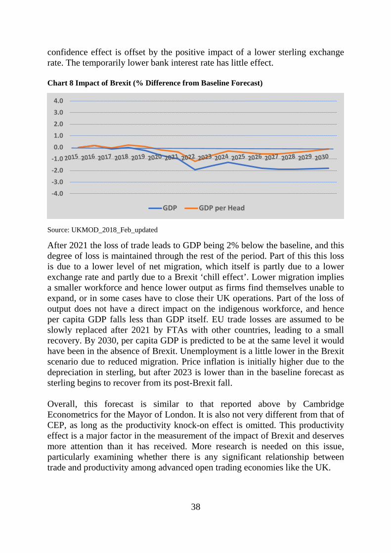
38
confidence effect is offset by the positive impact of a lower sterling exchange rate. The temporarily lower bank interest rate has little effect. Chart 8 Impact of Brexit (% Difference from Baseline Forecast)
Source: UKMOD_2018_Feb_updated
After 2021 the loss of trade leads to GDP being 2% below the baseline, and this degree of loss is maintained through the rest of the period. Part of this this loss is due to a lower level of net migration, which itself is partly due to a lower exchange rate and partly due to a Brexit ‘chill effect’. Lower migration implies a smaller workforce and hence lower output as firms find themselves unable to expand, or in some cases have to close their UK operations. Part of the loss of output does not have a direct impact on the indigenous workforce, and hence per capita GDP falls less than GDP itself. EU trade losses are assumed to be slowly replaced after 2021 by FTAs with other countries, leading to a small recovery. By 2030, per capita GDP is predicted to be at the same level it would have been in the absence of Brexit. Unemployment is a little lower in the Brexit scenario due to reduced migration. Price inflation is initially higher due to the depreciation in sterling, but after 2023 is lower than in the baseline forecast as sterling begins to recover from its post-Brexit fall. Overall, this forecast is similar to that reported above by Cambridge Econometrics for the Mayor of London. It is also not very different from that of CEP, as long as the productivity knock-on effect is omitted. This productivity effect is a major factor in the measurement of the impact of Brexit and deserves more attention than it has received. More research is needed on this issue, particularly examining whether there is any significant relationship between trade and productivity among advanced open trading economies like the UK.
-4.0
-3.0
-2.0
-1.0
0.0
1.0
2.0
3.0
4.0
GDP GDP per Head

39
7. Concluding Comments
In this paper, we have reviewed economists’ assessments of the economic performance of the UK within the EU, and the short-term and long-term economic effects of the referendum decision to leave the EU. Many of these assessments have been by government departments and international agencies. In estimating the economic effects of Brexit on living standards, these rely on a range of analytic approaches, including the use of gravity models, computable general equilibrium models and macroeconomic forecasting models. Our conclusion is that much of this work contains flaws of analysis, and a treatment of evidence that leads to exaggerated costs of Brexit. Gravity models are well established as a technique for estimating the impact of trade associations or currency unions but require more care than has been in shown, when being applied to a specific issue like Brexit. The Treasury has been particularly cavalier in its approach, both in its application of gravity analysis and in applying a ‘knock-on’ impact from trade to productivity. Other organisations have been a little more circumspect about the productivity link, which we doubt exists to any significant degree for advanced economies, but several have used it without much questioning. The short-term forecasts which have turned out to be wrong have further damaged confidence in economists’ contributions to public debate. Partly as a result, very little attention is currently being given by politicians or the public on either side of the debate to the impact assessments published at the time of the referendum. The potential damage to the UK’s negotiating position on Brexit may have been limited by the indifference of policy-makers to economic impact assessments. Although the UK government has steered away from further work on economic assessments of Brexit, devolved governments have felt less constrained. The Mayor of London, reacting against the UK Government’s reluctance to publish assessments, commissioned Cambridge Econometrics, who showed that a modelling approach without gravity models or general equilibrium, will generate moderate and plausible results. Even so, only the most pessimistic of their conclusions on Brexit received any publicity. CE’s gave little attention to their prediction that per capita GVA was little changed by Brexit and hence the media ignored it. The Scottish Government was much less inhibited and ploughed ahead with an analysis incorporating all of the flaws in the Treasury and CEP analyses with no acknowledgement of published criticisms. The consequences of these shortcomings go well beyond Brexit itself. We believe that the credibility of the economic forecasting profession and some of the major parts of the economic press, have been damaged again. It will take
40
more than a decade to be sure of this, but the failure of the short-term forecasts indicates what could happen. The fact that the flaws we identify all point in the direction of pessimism on Brexit, and hence in the direction that most academics and economists tend to lean ideologically, will increase the scepticism of many. The refusal of the Treasury to discuss their approach, at least until the issue was aired in Parliament, is in our view unacceptable in an open democracy. Our conclusion is that in order to restore public confidence in economic forecasting for major policy issues like Brexit, economists need to use more relevant analyses, based on a wider range of evidence. We expect that econometric models used by commercial forecasters like Cambridge Econometrics, will prove to be most accurate in the long-run. If so, the academic profession needs to reconsider both the relevance of its current attachment to theory based on unrealistic assumptions, and to the general quality of policy-relevant applied work. Whatever techniques are used need to be applied with more balance and scepticism. The CEP in discussing the Treasury reports could only think of changes which would have made the HMT predictions even more pessimistic on Brexit. In the words of Oliver Cromwell to the General Assembly of the Church of Scotland, the economic forecasting profession needs to ‘think it possible ye may be mistaken’.

41
Notes 1 ‘Membership of the EU has contributed to the economic prosperity of the UK. Since 1973, when the UK joined the EU, UK GDP per capita doubled, increasing more than in other non-EU English speaking countries over the same period, including in the United States (US). Domestic policies partly explain this strong performance, but geographic proximity and unrestricted access to the largest market in the world are undeniably important factors as well. For smaller countries with competitive markets the benefits could be even larger. For example, Ireland, which also joined the European Union in 1973, had a near quadrupling of its GDP per capita’. OECD (April 2016). This claim for gains from EEC/EU membership is vague. The claim of growth faster than the USA is refuted if GDP in the USA is adjusted for the impact of mispricing of IT production (see Conference Board, 2017). The reference to Ireland omits any mention of that country’s tax haven status and the associated gross distortion of its GDP statistics. 2 In his section 2 ‘The Impact of EU Membership on the UK GDP’, Crafts reviews a range of academic literature. However, some of this does not relate directly to the EU, or takes an average estimate of EU membership on UK economic growth which is not specific to the UK. An exception is Campos et al (2014) which uses a counterfactual scenario based on benchmark countries to calculate what might have occurred in the absence of joining the EU. The calculation that per capita GDP in the UK would have been 23.7% higher was based on New Zealand and Argentina as benchmarks. Our view is that not much can be learnt from comparing the UK with New Zealand and Argentina before and after 1973, and we discount this evidence. See also Broadberry and Crafts (2010) who make similar points in their section 4. Other evidence relates to improvements to competitiveness in UK manufacturing related to openness but not specifically to the EU. 3 Crafts also adds: ‘EU membership has raised trade and income levels in the UK in the past through increasing economic integration. It seems quite clear that these gains have outweighed the “membership fee” which has primarily consisted of budget transfers and costly regulation. When the UK entered the EU in 1973 it was after a period of serious underperformance in economic growth which had seen income and productivity levels fall behind those of France and West Germany. The trade liberalization and concomitant increase in competitive pressures associated with EU entry was an appropriate policy response to relative economic decline especially given the importance of competition for the effective functioning of the

42
“liberal market economy” variety of capitalism’ (Crafts, 2016: 12). 4 Mark Carney, Governor of the Bank of England, Inflation Report Press Conference (May 2016). Christine Lagarde, IMF Managing Director, Press conference for the IMF UK Article IV concluding statement (May 2016). 5 National Institute Global Econometric Model. https://nimodel.niesr.ac.uk/ 6 The Costs and Benefits of Leaving the EU: the Trade Effects. CEP Discussion Paper No 1478 April 2017. For brevity, we refer to the authors: Dhingra, Huang, Ottaviano, Pessoa, Sampson and van Reenan as Dhingra et al. 7 The CGE model is divided into 35 world regions; each region is disaggregated into 31 industrial sectors for goods and services. The data consists of bilateral trade relationships between each region and sector, using the United Nations COMTRADE data base. The inter-sectoral relationships use the WIOD input-output tables from the European Commission (see Timmer et al. (2015)). 8 Dhingra et al. quote their results from the working paper by Méjean and Schwellnus. In the published version, Table 1, column (3) gives a convergence rate for OECD countries of 0.584 (=1-0.416) for OECD countries and 0.394 for EU countries. 9 The figures are taken from Table 3D, central estimates, paragraph 3.56, pages 138 H M Treasury (2016ba) 10 Imbs and Méjean (2016) define their sectors at the ISIC 2-digit level. 11https://www.london.gov.uk/sites/default/files/preparing_for_brexit_final_report.pdf 12 https://www.cbr.cam.ac.uk/fileadmin/user_upload/centre-for-business-research/downloads/working-papers/wp483.pdf 13 Our critique can be seen at: https://www.cbr.cam.ac.uk/fileadmin/user_upload/centre-for-business-research/downloads/working-papers/wp490.pdf/

43
References
Armington, P. S., (1969), A Theory of Demand for Products Distinguished by Place of Production, Staff Papers, International Monetary Fund.
Baier, S. L., Bergstrand, J. H., Egger, P., McLaughlin, P. H., (2008), Do Economic Integration Agreements Actually Work? Issues in Understanding the Causes and Consequences of the Growth of Regionalism, The World Economy, vol 31, (4), 461-497.
Berden, K., François, J., Taminen, S., Thelle, M., and Wymenga, P., (2009), Non-tariff Measures in EU-US Trade and Investment: An Economic Analysis, Final Report, Ecorys.
_______ (2013), Non-tariff Measures in EU-US Trade and Investment: An Economic Analysis, IIDE Discussion Papers, 20090806, Institute for International and Development Economics.
Broadberry, S., and Crafts, N., (2010), Openness Protection and Britain’s Productivity Performance over the long-run. University of Warwick Working paper series no. 36.
Caliendo, L., and Parro, F., (2015), Estimates of the Trade and Welfare Effects of NAFTA, Review of Economic Studies, vol 82, (1), 1-44.
Campos, N., Coricelli, F. and Moretti, L., (2014), Economic Growth and Political Integration: Estimating the Benefits from Membership of the European Union using the Synthetic Counterfactuals Method, CEPR Discussion Paper No. 9968.
Cambridge Econometrics, (2018), Preparing for Brexit, Report for Greater London Authority, January.

44
Clarke, H. D., Goodwin, M. and Whiteley, P., (2017), Brexit:Why Britain Voted to Leave the European Union. CUP.
Costinot, A., and Rodríguez-Clare, A., (2014), Trade Theory with Numbers: Quantifying the Consequences of Globalisation, vol 4, Handbook of International Economics, Elsevier.
Crafts, N., (2016), The Growth Effects of EU Membership for the UK: A Review of the Evidence, Social market Foundation Global Perspectives Series Paper 7.
Dhingra, S., Ottaviano,G., Sampson, T., and van Reenan, J., (2016), The UK
Treasury Analysis of ‘The long-term economic impact of UK membership and the alternatives’: CEP Commentary, Brexit Paper 04.
Dhingra, S., Huang, H., Ottaviano,G., Pessoa, J. P., Sampson, T., and van Reenan, J., (2017), The Costs and Benefits of Leaving the EU: the Trade Effects. CEP Discussion Paper No 1478 April.
Eaton, J., and Kortum, S., (2002), Technology, Geography and Trade, Econometrica, vol 70, (5), 1741-1779.
Ebell M Hurst I and Warren J, (2016) Modelling the Long-term economic Impact of leaving the European Union. NIESR Discussion Paper 462 June 2016.
Feyrer, J., (2009a), Trade and Income – Exploiting Time Series in Geography, NBER Working Papers, 14910, National Bureau of Economic Research, Inc.
Feyrer, J., (2009b), Distance, Trade and Income-The 1968-75 Closing of the Suez Canal as a natural Experiment. NBER Working Paper 15557 Dec 2009.

45
Fournier, J. et al. (2015), ‘Implicit Regulatory Barriers in the EU Single Market: New Empirical Evidence from Gravity Models’, OECD Economics Department Working Papers, No. 1181, OECD Publishing, Paris.
Gudgin G, Coutts K, Gibson N (2015) The CBR Macro-Economic Model of the
UK Economy. Centre for Business Research, University of Cambridge Working Paper No. 472
Gudgin G, Coutts K, Gibson N, and Buchanan J (2017a) The Role of Gravity
Models in estimating the Economic Impact of Brexit. Centre for Business Research, University of Cambridge Working Paper No. 490 https://www.cbr.cam.ac.uk/fileadmin/user_upload/centre-for-business-research/downloads/working-papers/wp490.pdf/
Gudgin G, Coutts K, Gibson N, and Buchanan J (2017b) defying Gravity. A Critique of estimates of the Economic Impact of Brexit. Policy Exchange. London. https://policyexchange.org.uk/wp-content/uploads/2017/06/Defying-Gravity-A-critique-of-estimates-of-the-economic-impact-of-Brexit.pdf/
H. M. Treasury, (2005), EU Membership and Trade. Internal Paper Unclassified. (Authors unknown) https://www.gov.uk/government/uploads/system/uploads/attachment_data/file/220968/foi_eumembership_trade.pdf/
H. M. Treasury, (2016a), H M Treasury Analysis: the long-term economic impact of UK membership and the alternatives, CM 9250, April. https://www.gov.uk/government/uploads/system/uploads/attachment_data/file/517415/treasury_analysis_economic_impact_of_eu_membership_web.pdf/

46
H. M. Treasury, (2016b), The immediate economic impact of leaving the EU. Cmnd 9292. May. https://www.gov.uk/government/uploads/system/uploads/attachment_data/file/524967/hm_treasury_analysis_the_immediate_economic_impact_of_leaving_the_eu_web.pdf/
Imbs, J., and Méjean, I., (2017), Trade Elasticities, Review of International Economics, vol 25, issue 2, May, 383-402.
Institute of Fiscal Studies, (2016), Brexit and the UK’s Public Finances.
Keck, A. and Lendle, A., (2012), New Evidence on Preference Utilisation, World Trade Organisation, Staff Working Paper, ERSD 2012-12.
Kee, Nicita and Olarreaga (2009) Estimating Trade Restrictiveness Indices. Economic Journal. 2009. Vol 119 p.172-199
Kee, H. L. and Nicita, A., (2017), Short Term Impact of Brexit on the UK’s Exports of Goods. Vox Blog, World Bank and UNCTAD.
Lawless, M. and Morgenroth, E, (2016), The Product and Sector level Impact of a Hard Brexit across the EU, ESRSI, working Paper no. 550, November.
Lawless, M. and Studnicka, Z., (2017), Potential Impact of WTO Tariffs on Cross-border Trade, InterTradeIreland, June.
Mayer, M., Hautz, J., Stadler, C., Whittington, R., (2017), While Corporate UK was for Remain, Their Business Strategies tell a Different Story, LSE, Politics and Policy, http://blogs.lse.ac.uk/politicsandpolicy/a-close-look-at-british-business-was-it-destined-to-leave-the-eu/#Author/

47
Melitz, M. and Trefler, D., (2012), The Gains from Trade when Firms Matter, Journal of Economic Perspectives, vol 26, issue 2, 91-118.
Méjean, I., and Schwellnus, C., (2009), Price Convergence in the European Union: Within Firms or Composition of Firms? Working Papers, hal-00354190, HAL.
Mulabdic, A., Osnago, A., and Ruta, M., (2017), Deep Integration and UK- EU Trade Relations, Policy Research Working Paper Series 7947, The World Bank.
OECD, (2016), The Economic Consequences of Brexit: A Taxing Decision. OECD Economic Policy Paper No. 16, April.
Ottaviano, G., (2014), European Integration and the Gains from Trade, Centre for Financial Studies, Working Paper 470, September.
Sampson, T., (2016), Dynamic Selection: An Idea Flows Theory of Entry, Trade and Growth, The Quarterly Journal of Economics, vol 131, issue 1, 315.
Timmer, M. P., Dietzenbacher, E., Los, B., Stehrer, R. and de Vries, G. J., (2015), An Illustrated User Guide to the World Input-Output Database: the Case of Global Automotive Production, Review of International Economics, vol 23, 575-605.
Walsh, K., (2006), Trade in Services: Does Gravity Hold? A Gravity Model Approach to Estimating Barriers to Services, Trade. Discussion Paper Series, no 183, Revenue Commissioners Dublin.

48
Appendix A Equations for Impact of EU membership on Growth in per capita GDP in the UK
The following equations fitted over the period 1960-2016 include a range of statistically significant influences on the annual growth rate of per capita GDP in the UK. They also include dummy variables for EU membership. One of these (D_EU_70s) covers the difficult early period 1973-77 during which the UK was aligning its tariff regime to that of the UK. Average tariffs changed relatively little, but these were difficult years for both the UK and world economies following the quadrupling of word oil prices in 1973 and subsequent recession in many economies. Many other important factors influenced growth. One was high wage inflation followed by a wage freeze from 1976, Another was the steady build-up of North Sea Oil production. Dependent Variable: DLOG(GDPV_0) Method: Least Squares Date: 10/31/17 Time: 10:37 Sample: 1960 2016 Included observations: 57
Variable Coefficient Std. Error t-Statistic Prob.
C 1.956272 0.607969 3.217716 0.0025 LOG(GDPV(-1)) -0.152684 0.048381 -3.155857 0.0029
LOG(WTI) 0.052686 0.018949 2.780382 0.0080 NUMLOANS(-1)/POPW(-1) 0.000916 0.000205 4.465667 0.0001
D(TAX_CTRATE(-1)) -0.002854 0.000607 -4.703320 0.0000 DLOG(GDPV(-2)) -0.412188 0.062409 -6.604609 0.0000
DLOG(ER) 0.933855 0.107698 8.671076 0.0000 D_EEC_70S -0.020354 0.005384 -3.780474 0.0005
D_EEC2 -0.002467 0.005093 -0.484277 0.6306 DLOG(TAX_CTRATE) 0.123212 0.026554 4.640123 0.0000
D69 -0.019712 0.008312 -2.371479 0.0223 D80 -0.033778 0.008598 -3.928582 0.0003 D84 -0.021639 0.008894 -2.432891 0.0192
D2009 -0.025507 0.009867 -2.584997 0.0132
R-squared 0.888489 Mean dependent var 0.024069 Adjusted R-squared 0.854776 S.D. dependent var 0.020853 S.E. of regression 0.007947 Akaike info criterion -6.622772 Sum squared resid 0.002715 Schwarz criterion -6.120970 Log likelihood 202.7490 Hannan-Quinn criter. -6.427755 F-statistic 26.35473 Durbin-Watson stat 1.953323 Prob(F-statistic) 0.000000

49
Another EU dummy variable (D_EU2) covers the period 1978-2016, i.e. the period in which UK trade policy was fully aligned with the EEC/EU. In the first equation below the D_EU_70s dummy variable is significant and negative, no doubt reflecting the difficult world economic conditions of this period. The main D_EU2 dummy is negative but non-significant. However, small changes in specification, in the second equation, reverse this conclusion. In this case D_EU_70s is not significant but D_EU2 is significant and positive indicating an ongoing advantage from membership of the EU. The third equation shows that this advantage only occurs in the period prior to 1992, and hence before the Maastrict Treaty which led to acceleration in regulatory convergence.
Dependent Variable: DLOG(GDPV) Method: Least Squares Date: 01/13/18 Time: 15:18 Sample (adjusted): 1961 2016 Included observations: 56 after adjustments
Variable Coefficient Std. Error t-Statistic Prob. C 3.633030 0.971626 3.739122 0.0005
LOG(GDPV(-1)) -0.287008 0.075058 -3.823792 0.0004 LOG(WTI) 0.095367 0.026218 3.637405 0.0007
LR(-1) -0.002134 0.001041 -2.050231 0.0465 TAX_CTRATE(-1) -0.001723 0.000485 -3.552142 0.0009 NUMLOANS(-1) 4.44E-08 6.14E-09 7.226522 0.0000
DLOG(GDPV(-2)) -0.339730 0.070046 -4.850108 0.0000 DLOG(NUMLOANS) 0.025305 0.007147 3.540479 0.0010
TAX_INC_BASIC_RATE(-1) 0.003295 0.001379 2.390188 0.0213 D(TAX_INC_TOP_RATE) -0.000352 0.000278 -1.267712 0.2117
D_EEC_70S 0.008778 0.009266 0.947366 0.3487 D_EEC2 0.025280 0.010294 2.455826 0.0182
D(ER) 0.007356 0.001996 3.685902 0.0006 R-squared 0.858462 Mean dependent var 0.023510
Adjusted R-squared 0.818963 S.D. dependent var 0.020306 S.E. of regression 0.008640 Akaike info criterion -6.464687 Sum squared resid 0.003210 Schwarz criterion -5.994516 Log likelihood 194.0112 Hannan-Quinn criter. -6.282402 F-statistic 21.73376 Durbin-Watson stat 2.336400 Prob(F-statistic) 0.000000
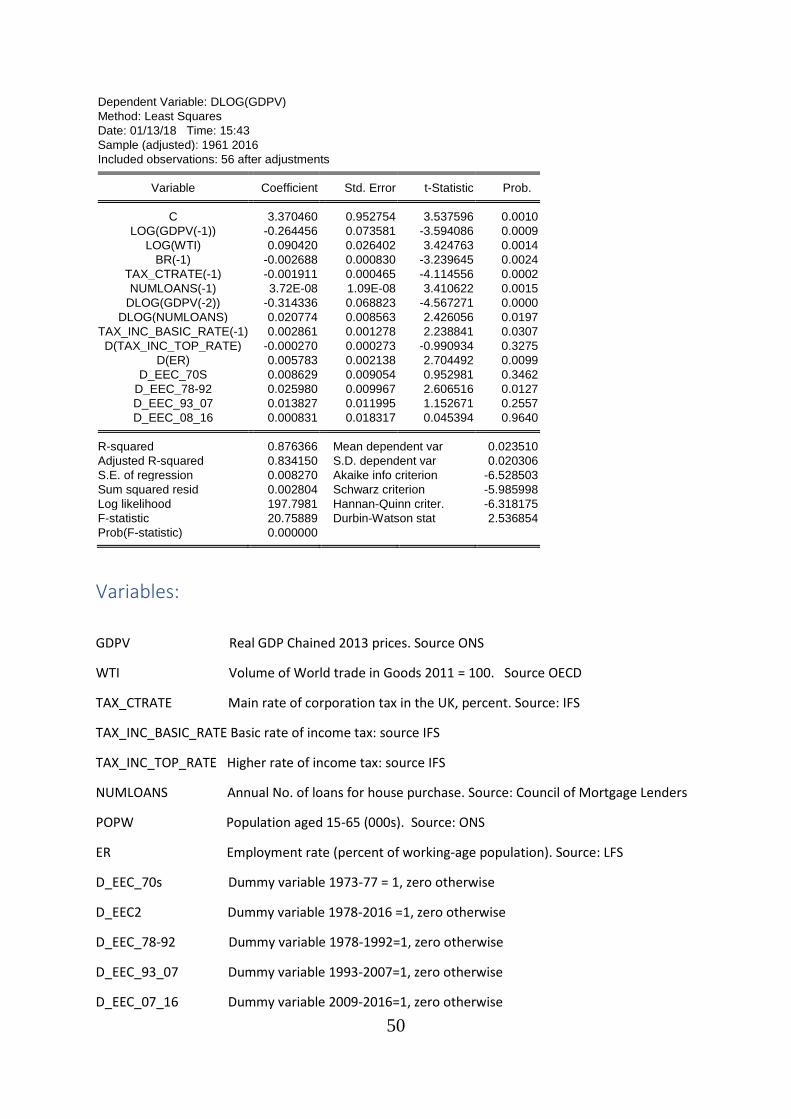
50
Dependent Variable: DLOG(GDPV) Method: Least Squares Date: 01/13/18 Time: 15:43 Sample (adjusted): 1961 2016 Included observations: 56 after adjustments
Variable Coefficient Std. Error t-Statistic Prob. C 3.370460 0.952754 3.537596 0.0010
LOG(GDPV(-1)) -0.264456 0.073581 -3.594086 0.0009 LOG(WTI) 0.090420 0.026402 3.424763 0.0014
BR(-1) -0.002688 0.000830 -3.239645 0.0024 TAX_CTRATE(-1) -0.001911 0.000465 -4.114556 0.0002 NUMLOANS(-1) 3.72E-08 1.09E-08 3.410622 0.0015
DLOG(GDPV(-2)) -0.314336 0.068823 -4.567271 0.0000 DLOG(NUMLOANS) 0.020774 0.008563 2.426056 0.0197
TAX_INC_BASIC_RATE(-1) 0.002861 0.001278 2.238841 0.0307 D(TAX_INC_TOP_RATE) -0.000270 0.000273 -0.990934 0.3275
D(ER) 0.005783 0.002138 2.704492 0.0099 D_EEC_70S 0.008629 0.009054 0.952981 0.3462
D_EEC_78-92 0.025980 0.009967 2.606516 0.0127 D_EEC_93_07 0.013827 0.011995 1.152671 0.2557 D_EEC_08_16 0.000831 0.018317 0.045394 0.9640
R-squared 0.876366 Mean dependent var 0.023510
Adjusted R-squared 0.834150 S.D. dependent var 0.020306 S.E. of regression 0.008270 Akaike info criterion -6.528503 Sum squared resid 0.002804 Schwarz criterion -5.985998 Log likelihood 197.7981 Hannan-Quinn criter. -6.318175 F-statistic 20.75889 Durbin-Watson stat 2.536854 Prob(F-statistic) 0.000000
Variables:
GDPV Real GDP Chained 2013 prices. Source ONS
WTI Volume of World trade in Goods 2011 = 100. Source OECD
TAX_CTRATE Main rate of corporation tax in the UK, percent. Source: IFS
TAX_INC_BASIC_RATE Basic rate of income tax: source IFS
TAX_INC_TOP_RATE Higher rate of income tax: source IFS
NUMLOANS Annual No. of loans for house purchase. Source: Council of Mortgage Lenders
POPW Population aged 15-65 (000s). Source: ONS
ER Employment rate (percent of working-age population). Source: LFS
D_EEC_70s Dummy variable 1973-77 = 1, zero otherwise
D_EEC2 Dummy variable 1978-2016 =1, zero otherwise
D_EEC_78-92 Dummy variable 1978-1992=1, zero otherwise
D_EEC_93_07 Dummy variable 1993-2007=1, zero otherwise
D_EEC_07_16 Dummy variable 2009-2016=1, zero otherwise

51
Appendix B
Comparative static properties of an Armington model
To gain a clearer understanding of the technical analysis which underlies the static effects of Brexit, we discuss in more detail the general equilibrium model on which the analysis is based. Consumption preferences for each country are given by the CES specification:
𝐶𝐶𝑗𝑗 = ���𝐶𝐶𝑖𝑖𝑗𝑗𝜓𝜓𝑖𝑖𝑗𝑗
�
𝜎𝜎−1𝜎𝜎
𝑛𝑛
𝑖𝑖=1
�
𝜎𝜎𝜎𝜎−1
(1)
where 𝐶𝐶𝑗𝑗 is the consumption of country j, 𝐶𝐶𝑖𝑖𝑗𝑗 are country j’s consumption from country i, 𝜓𝜓𝑖𝑖𝑗𝑗 are consumption preference parameters and 𝜎𝜎 is the elasticity of substitution. Aggregate expenditure is defined as:
𝑃𝑃𝑗𝑗𝐶𝐶𝑗𝑗 = �𝑃𝑃𝑖𝑖𝑗𝑗𝐶𝐶𝑖𝑖𝑗𝑗 = 𝐸𝐸𝑗𝑗 (2)𝑛𝑛
𝑖𝑖=1
Maximisation of (1) subject to this budget constraint leads to a corresponding price index:
𝑃𝑃𝑗𝑗 = ���𝜓𝜓𝑖𝑖𝑗𝑗𝑃𝑃𝑖𝑖𝑗𝑗�1−𝜎𝜎
𝑛𝑛
𝑖𝑖=1
�
11−𝜎𝜎
(3)
It is also straightforward to derive the associated gravity equation:
𝑋𝑋𝑖𝑖𝑗𝑗 = �𝜓𝜓𝑖𝑖𝑗𝑗𝑃𝑃𝑖𝑖𝑗𝑗𝑃𝑃𝑗𝑗
�1−𝜎𝜎
𝐸𝐸𝑗𝑗 (4)
Note that the total expenditure by country j on imports plus its own purchase of domestic production is: 𝐸𝐸𝑗𝑗 = ∑ 𝑋𝑋𝑖𝑖𝑗𝑗𝑛𝑛
𝑖𝑖=1 . Trade frictions are Samuelson’s iceberg type –country i has to ship 𝜏𝜏𝑖𝑖𝑗𝑗 ≥ 1 units of its good to land one unit at the destination country. There are ad-valorem tariffs, 𝑡𝑡𝑖𝑖𝑗𝑗 ≥ 0. This implies:
𝑃𝑃𝑖𝑖𝑗𝑗𝑄𝑄𝑖𝑖 = �1 + 𝑡𝑡𝑖𝑖𝑗𝑗�𝜏𝜏𝑖𝑖𝑗𝑗𝑃𝑃𝑖𝑖𝑖𝑖𝑄𝑄𝑖𝑖
The landed price of a good from country j landed in county i is higher than the domestic price by the tariff and the trade friction cost. Income is defined as:
𝑌𝑌𝑖𝑖 = 𝑃𝑃𝑖𝑖𝑖𝑖𝑄𝑄𝑖𝑖, so 𝑃𝑃𝑖𝑖𝑗𝑗 = 𝜙𝜙𝑖𝑖𝑗𝑗𝑌𝑌𝑖𝑖𝑄𝑄𝑖𝑖� where 𝜙𝜙𝑖𝑖𝑗𝑗 = �1 + 𝑡𝑡𝑖𝑖𝑗𝑗�𝜏𝜏𝑖𝑖𝑗𝑗.
The whole system of n endogenous levels of income, 𝑌𝑌𝑖𝑖 , can be solved by n non-linear equations. Once the income levels are determined, prices can similarly be solved. From price information, the trade flows and the

52
expenditures can also be solved. From these, the consumption levels can be solved, which are used as the measure of welfare in the subsequent analysis. The important point to note is that this solution depends on providing values for the production in each country, 𝑄𝑄𝑖𝑖, the consumer preference parameters and the elasticity of substitution. One reason for the increasing popularity of NQTM models by trade economists is the limited number of pieces of information that are required to do counter-factual analysis. Changes in consumption can be calculated when comparing a change in trade costs from actual, 𝜙𝜙𝑖𝑖𝑗𝑗 , to counter-factual, 𝜙𝜙′𝑖𝑖𝑗𝑗 . Using only
information on actual and counter-factual trade shares, 𝜆𝜆𝑖𝑖𝑗𝑗 = 𝑋𝑋𝑖𝑖𝑗𝑗𝐸𝐸𝑗𝑗� , and the
trade elasticity parameter, 𝜀𝜀 = 𝜎𝜎 − 1 , changes in welfare as measured by consumption can be evaluated. CEP works with a single factor of production, 𝐸𝐸𝑗𝑗 = 𝑤𝑤𝑗𝑗𝐿𝐿𝑗𝑗 and solve for unknown wages instead of incomes. Ottaviano 2014 demonstrates the comparative static property of the above model. It can be shown that the welfare change:
�̂�𝐶𝑗𝑗 =1 − 𝜋𝜋𝑗𝑗1 − 𝜋𝜋′𝑗𝑗
��̂�𝜆𝑗𝑗𝑗𝑗�−1𝜀𝜀
where
𝜋𝜋𝑗𝑗 = �𝑡𝑡𝑖𝑖𝑗𝑗
1 + 𝑡𝑡𝑖𝑖𝑗𝑗𝜆𝜆𝑖𝑖𝑗𝑗 and 𝜋𝜋′𝑗𝑗 = �
𝑡𝑡′𝑖𝑖𝑗𝑗1 + 𝑡𝑡′𝑖𝑖𝑗𝑗
𝑛𝑛
𝑖𝑖=1
𝜆𝜆𝑖𝑖𝑗𝑗𝜆𝜆′𝑖𝑖𝑗𝑗 𝑛𝑛
𝑖𝑖=1
The hat over a variable shows the ratio of the new to initial value of that variable. The counter-factual values will depend on tariff and non-tariff inputs and initial and counter-factual expenditure shares. A further level of complexity is introduced by disaggregating trade by country into industrial sectors. The single elasticity parameter, 𝜎𝜎 , is replaced by elasticities for each sector. The corresponding formula takes the form:
�̂�𝐶𝑗𝑗 =1 − 𝜋𝜋𝑗𝑗1 − 𝜋𝜋′𝑗𝑗
���̂�𝜆𝑗𝑗𝑗𝑗�−𝛽𝛽𝑗𝑗,𝑠𝑠𝑎𝑎�𝑗𝑗,𝑠𝑠𝑠𝑠
𝜀𝜀𝑠𝑠
𝑆𝑆
𝑠𝑠,𝑘𝑘=1
Two further sets of data are introduced. The β coefficients are shares of sectoral output in household expenditure. The 𝑎𝑎�𝑗𝑗,𝑠𝑠𝑘𝑘 are the elements of the inverse of matrix �1 − 𝐴𝐴𝑗𝑗�
−1 and are described on page 12 as the elasticity of the price index in sector s with respect to changes in the price of sector k. The final

53
complication is that the calculation of welfare change is treated as the discounted permanent flow of consumption losses as discussed in the main text.
Appendix C Quantifying the implications of the UK not benefitting from future intra-EU trade cost declines The third element in the counter-factual scenarios, after tariffs and non-tariff barriers, is the assumption that future intra-EU trade costs will continue to decline while this will not happen when the UK is no longer a member of the single market. The CEP makes a number of assumptions about this effect and takes figures from several studies. CEP use results from Méjean and Schwellnus (2009) on the extent to which there is faster convergence of price differences for similar products within the EU than for exports outside the EU to OECD countries. CEP takes a figure from Table II of Eaton and Kortum (2002) which they take to represent the extent to which there are price differences for UK imports depending on the source. CEP takes a figure from their paper, Table 2, sourced from Berden et al. (2009) as to the percent of non-tariff barriers that are reducible and assume that the same percentage applies to the price differences quoted in Eaton and Kortum (2002). They further assume that in the pessimistic case (adoption of WTO rules), three-quarters of the reducible trade costs of UK-EU trade could be reduced. CEP quote rates of price convergence from Méjean and Schwellnus (2009) as -0.412 and -0.593 for OECD and EU countries respectively. These appear to be taken from Table 1, column (3), where the price convergence is -0.412 and -0.594. CEP appears to have dropped a third insignificant coefficient to use these figures. Column (2) specification gives the price convergence as -0.416 and -0.606 respectively. Whichever figures are used, it implies a faster convergence for EU compared with OECD countries of 44%-46%. It is worth noting that the implied rates of price convergence from the Méjean and Schwellnus (2009) paper are very rapid. The implied rates at which prices decline are 1-0.416=0.584 and 1-0.606=0.394 respectively. Their half-lives are given by: log�1
2� � = 𝑡𝑡 log(0.584) etc., giving 15 months for OECD countries and 9 months for EU countries. Turning to Eaton and Kortum (2002) for evidence on price differences, CEP takes a figure of UK prices being 49% higher than EU prices. This appears to be taken from Table II, but the figure given for the UK is 1.46 or 46% higher. What the table measures is that a UK resident who imported all goods from

54
abroad would face paying 46% more from the Netherlands, but would face paying 136% more if buying all goods from Japan. A resident abroad would pay 52% more for UK goods if living in France, but 104% more if living in New Zealand. CEP appears to have taken 49% as the average excess of price differences in different markets, though this is not clearly explained. The next step is that CEP assumes that the percent of non-tariff barriers that might be reducible, given in Berden et al. (2009), and referenced in CEP’s Table 2, also applies to price differences in different EU markets. The average weighted share given in the table is 54% of non-tariff barriers. They further assume that the reducible price difference, as proxied by non-tariff barriers, will be ¾ of the 54% assumed figure. The CEP calculation, given in their appendix B, is that the tariff equivalent of this reducible price difference in the pessimistic case is: 1 + 0.49*0.54*0.75 = 1.20. This compares with the tariff equivalent value of non-tariff barriers of 8.31%. The final step is to apply the approximately 44% faster convergence of prices from Méjean and Schwellnus (2009). The procedure is unclear in their appendix B, but CEP appears to have taken the excess convergence rate of 0.594 - 0.412 = 0.182 as the data for the speed of decay, which is 1 – 0.182. This rate of decay is applied to the 20% price excess (in the pessimistic case) for 10 years after which it is assumed to cease. Note that after 10 years the 20% rate will have decayed to 2.7%. In the text, CEP says that ‘future declines in intra-EU trade costs will reduce non-trade barriers within EU 10 years after Brexit by 12.65% and 5.63% in our pessimistic and optimistic scenarios, respectively’. They presumably meant to refer to future price reductions rather than non-tariff barriers. The average value of this price excess over 10 years is (20% + 2.7%)/2 = 11.4%, which is similar to the 12.65% given in the text. The key point is that this calculation gives a tariff equivalent effect that is 11.69% higher than the non-tariff barrier estimate at the exit from the EU and 5.61% lower after 10 years. For the first 5 years it is higher than the non-tariff barrier. Despite the weak foundations on which this reduction in future trade costs that the UK will miss on leaving the single market, this third static scenario result is quantitatively larger than the tariff and non-tariff barrier effects.

55