Embed Size (px)
Citation preview
DI
SC
US
SI
ON
P
AP
ER
S
ER
IE
S
Forschungsinstitut zur Zukunft der ArbeitInstitute for the Study of Labor
How the Demand for Labor May Adapt to the Availability of Labor: A Preliminary Exploration with Historical Data
IZA DP No. 8918
March 2015
Harriet Orcutt DuleepXingfei Liu
How the Demand for Labor May Adapt to the Availability of Labor: A Preliminary
Exploration with Historical Data
Harriet Orcutt Duleep College of William and Mary
and IZA
Xingfei Liu IZA
Discussion Paper No. 8918 March 2015
IZA
P.O. Box 7240 53072 Bonn
Germany
Phone: +49-228-3894-0 Fax: +49-228-3894-180
E-mail: [email protected]
Any opinions expressed here are those of the author(s) and not those of IZA. Research published in this series may include views on policy, but the institute itself takes no institutional policy positions. The IZA research network is committed to the IZA Guiding Principles of Research Integrity. The Institute for the Study of Labor (IZA) in Bonn is a local and virtual international research center and a place of communication between science, politics and business. IZA is an independent nonprofit organization supported by Deutsche Post Foundation. The center is associated with the University of Bonn and offers a stimulating research environment through its international network, workshops and conferences, data service, project support, research visits and doctoral program. IZA engages in (i) original and internationally competitive research in all fields of labor economics, (ii) development of policy concepts, and (iii) dissemination of research results and concepts to the interested public. IZA Discussion Papers often represent preliminary work and are circulated to encourage discussion. Citation of such a paper should account for its provisional character. A revised version may be available directly from the author.
IZA Discussion Paper No. 8918 March 2015
ABSTRACT
How the Demand for Labor May Adapt to the Availability of Labor: A Preliminary Exploration with Historical Data
This note presents and tests a general model to help explain why the demand for labor adapts to the availability of labor. In particular, we postulate that the cost of hiring declines with a growth in available labor for two reasons: (1) individuals seeking employment would be coming to employers instead of the latter seeking them out and (2) the larger set of potential employees would increase the probability of employers finding individuals suitable for unfilled jobs. Moreover, individuals seeking employment likely encourage employers to think of new ways in which labor can be used. An increase in the number of entrants to the labor force would lower the cost of hiring and increase employment demand at any given wage rate. Hence, a change in the labor force – such as the addition of women or immigrants – does not increase unemployment as much as is predicted for current workers because demand for labor increases as the cost of hiring decreases. Failure to taken into account what we term an – “encouraged employer effect” may also explain why surges in employment are often underestimated. JEL Classification: J20, J21, J23 Keywords: encouraged employer effect, hiring cost, labor demand, labor force Corresponding author: Xingfei Liu IZA Schaumburg-Lippe-Str. 5-9 53113 Bonn Germany E-mail: [email protected]
2
How the Demand for Labor May Adapt to the Availability of Labor: A Preliminary
Exploration with Historical Data
Harriet Duleep and Xingfei Liu
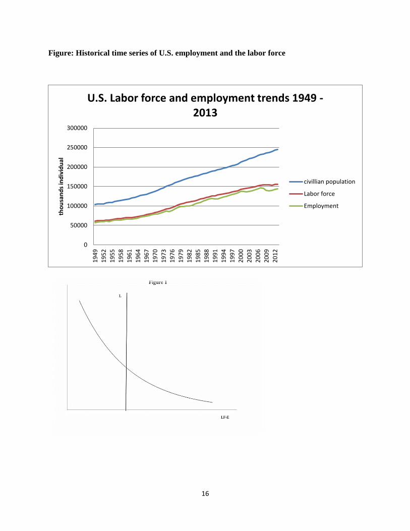
Labor supply is typically presented as a function of labor demand in economics text
books. Yet, as shown below, employment tracks the labor force. In this paper we posit a general
model of how labor demand responds to labor supply and test it with historical data.
[Figure: Historical time series of U.S. employment and the labor force]
I. The Model
We propose the following joint hypothesis: the cost of hiring declines with increases in
the amount of labor available for employment, and the employment decisions of firms are
inversely related to the cost of hiring.
The cost of hiring should decrease with a growth in the available labor supply (either new
entrants or unemployed individuals) for two reasons: individuals seeking employment would be
approaching employers instead of the latter seeking them out, and the larger set of potential
employees would increase the probability of employers finding suitable individuals for unfilled
jobs. Moreover, individuals seeking employment likely encourage employers to think of new
ways in which labor can be used. Employment inversely related to hiring costs rests on the
assumption that firms minimize costs.
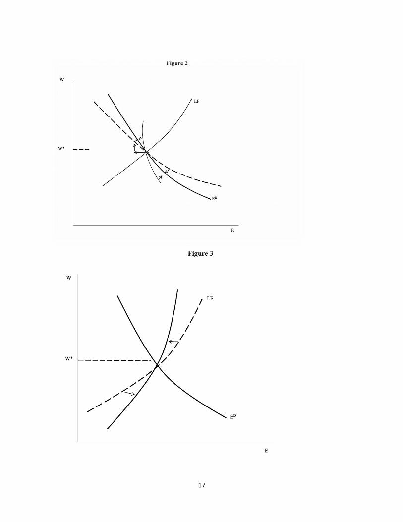
Figures 1 and 2 clarify these ideas. The cost of hiring, L, is a function of the number of
persons in the labor force minus the number employed, LF – E. The broken line in Figure 2
represents the traditionally conceived labor demand curve where employment decisions are a
3
function of the wage rate. The continuous line demonstrates the added effect of the cost of
hiring, L.
Starting at the equilibrium wage rate, W*, an increase in the wage rate decreases the
demand for employment. The increased wage increases the amount of labor available for
employment (LF – E), which lowers L. The lower value of L induces additional demand for
employment. And additional employment increases L. The process converges somewhere in
between, to the right of the original demand curve. Similarly, going below the equilibrium wage
rate increases L, which then decreases the demand for employment at any given wage rate.
A shift in the labor supply curve, LF, would also affect the cost of hiring in the same
way. For example, an increase in the number of entrants to the labor force would lower L and
increase employment demand at any given wage rate.
Insert Figure 1 and Figure 2 here.
A process symmetric to the cost-of-hiring effect occurs from the point of view of labor.
An increase in employment or a decrease in the labor force decreases the cost of finding a job,
which then increases the labor supply at any given wage rate (Figure 3). This has been referred to
as the ―discouraged worker effect.‖ We are proposing an ―encouraged employer effect.‖
Insert Figure 3 here.
The general state of the labor market is disequilibrium. We have assumed that observed
employment is the minimum of the demand and supply of labor. Referring back to Figure 2, the
demand for labor is only observed when the wage rate exceeds the equilibrium wage rate.
However, given the difficulty of determining an equilibrium wage rate, we simply assume that
4
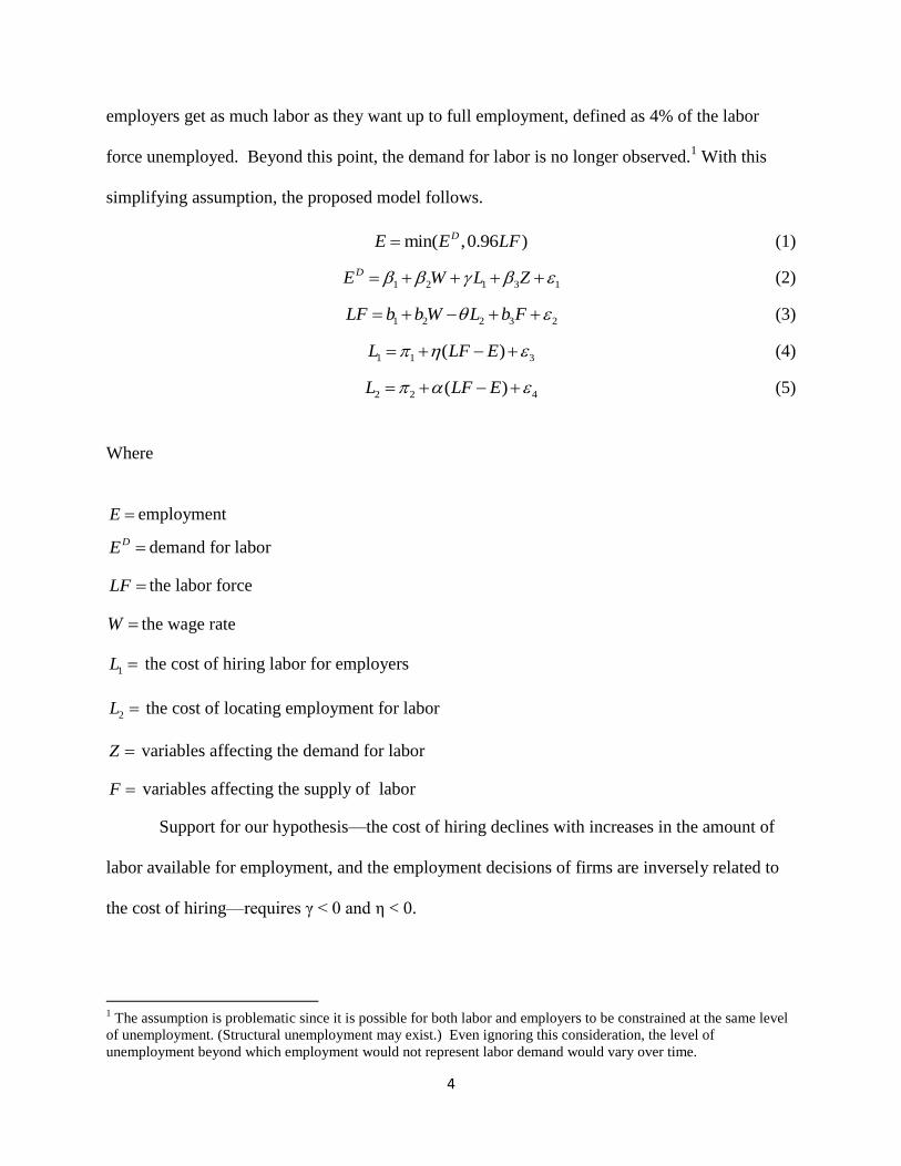
employers get as much labor as they want up to full employment, defined as 4% of the labor
force unemployed. Beyond this point, the demand for labor is no longer observed.1 With this
simplifying assumption, the proposed model follows.
min( ,0.96 )DE E LF (1)
1 2 1 3 1
DE W L Z (2)
1 2 2 3 2LF b b W L b F (3)
1 1 3( )L LF E (4)
2 2 4( )L LF E (5)
Where
E employment
DE demand for labor
LF the labor force
W the wage rate
1L the cost of hiring labor for employers
2L the cost of locating employment for labor
Z variables affecting the demand for labor
F variables affecting the supply of labor
Support for our hypothesis—the cost of hiring declines with increases in the amount of
labor available for employment, and the employment decisions of firms are inversely related to
the cost of hiring—requires γ < 0 and η < 0.
1 The assumption is problematic since it is possible for both labor and employers to be constrained at the same level
of unemployment. (Structural unemployment may exist.) Even ignoring this consideration, the level of
unemployment beyond which employment would not represent labor demand would vary over time.
5
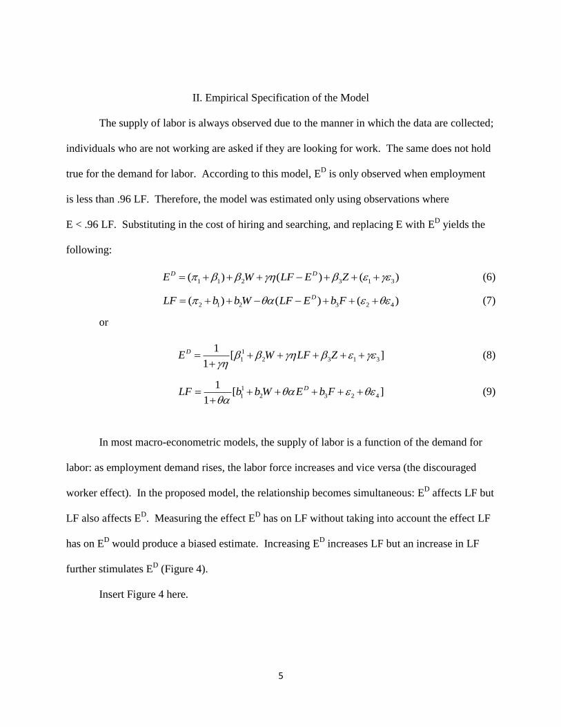
II. Empirical Specification of the Model
The supply of labor is always observed due to the manner in which the data are collected;
individuals who are not working are asked if they are looking for work. The same does not hold
true for the demand for labor. According to this model, ED is only observed when employment
is less than .96 LF. Therefore, the model was estimated only using observations where
E < .96 LF. Substituting in the cost of hiring and searching, and replacing E with ED yields the
following:
1 1 2 3 1 3( ) ( ) ( )D DE W LF E Z (6)
2 1 2 3 2 4( ) ( ) ( )DLF b b W LF E b F (7)
or
1
1 2 3 1 3
1[ ]
1
DE W LF Z
(8)
1
1 2 3 2 4
1[ ]
1
DLF b b W E b F
(9)
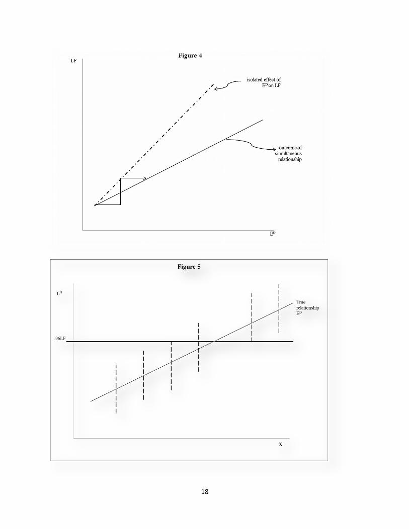
In most macro-econometric models, the supply of labor is a function of the demand for
labor: as employment demand rises, the labor force increases and vice versa (the discouraged
worker effect). In the proposed model, the relationship becomes simultaneous: ED affects LF but
LF also affects ED. Measuring the effect E
D has on LF without taking into account the effect LF
has on ED would produce a biased estimate. Increasing E
D increases LF but an increase in LF
further stimulates ED (Figure 4).
Insert Figure 4 here.
6
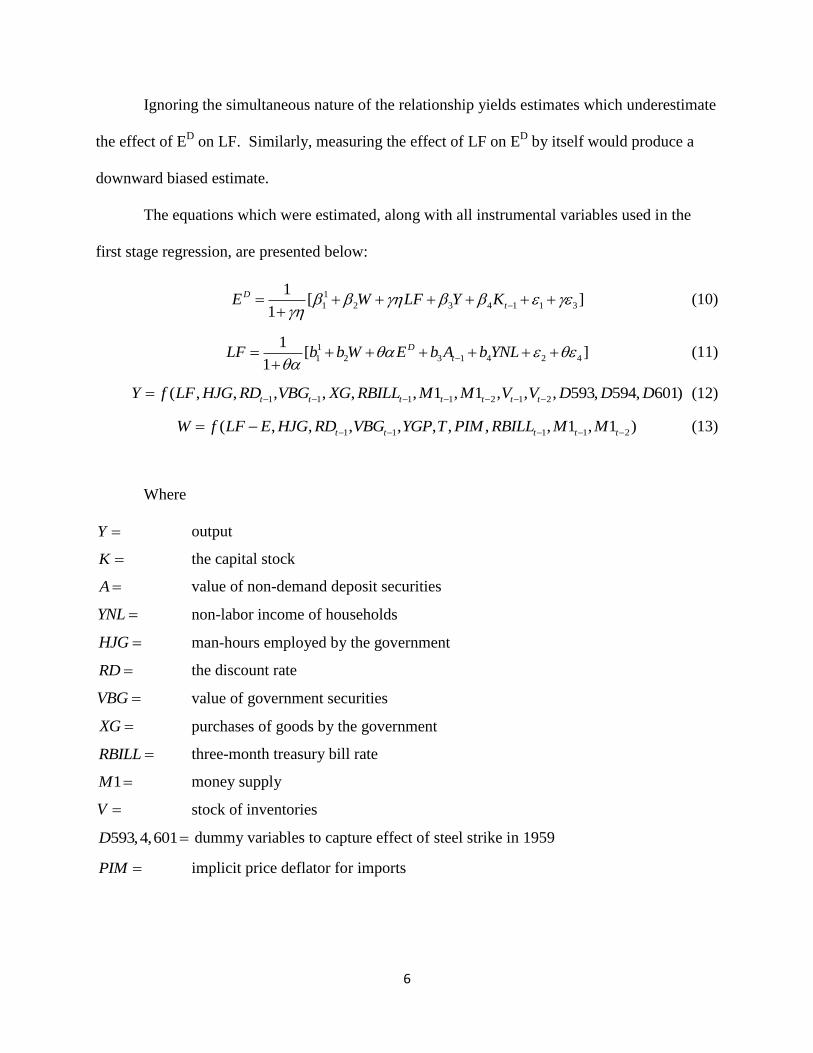
Ignoring the simultaneous nature of the relationship yields estimates which underestimate
the effect of ED on LF. Similarly, measuring the effect of LF on E
D by itself would produce a
downward biased estimate.
The equations which were estimated, along with all instrumental variables used in the
first stage regression, are presented below:
1
1 2 3 4 1 1 3
1[ ]
1
D
tE W LF Y K
(10)
1
1 2 3 1 4 2 4
1[ ]
1
D
tLF b b W E b A b YNL
(11)
1 1 1 1 2 1 2( , , , , , , 1 , 1 , , , 593, 594, 601)t t t t t t tY f LF HJG RD VBG XG RBILL M M V V D D D (12)
1 1 1 1 2( , , , , , , , , 1 , 1 )t t t t tW f LF E HJG RD VBG YGP T PIM RBILL M M (13)
Where
Y output
K the capital stock
A value of non-demand deposit securities
YNL non-labor income of households
HJG man-hours employed by the government
RD the discount rate
VBG value of government securities
XG purchases of goods by the government
RBILL three-month treasury bill rate
1M money supply
V stock of inventories
593,4,601D dummy variables to capture effect of steel strike in 1959
PIM implicit price deflator for imports
7
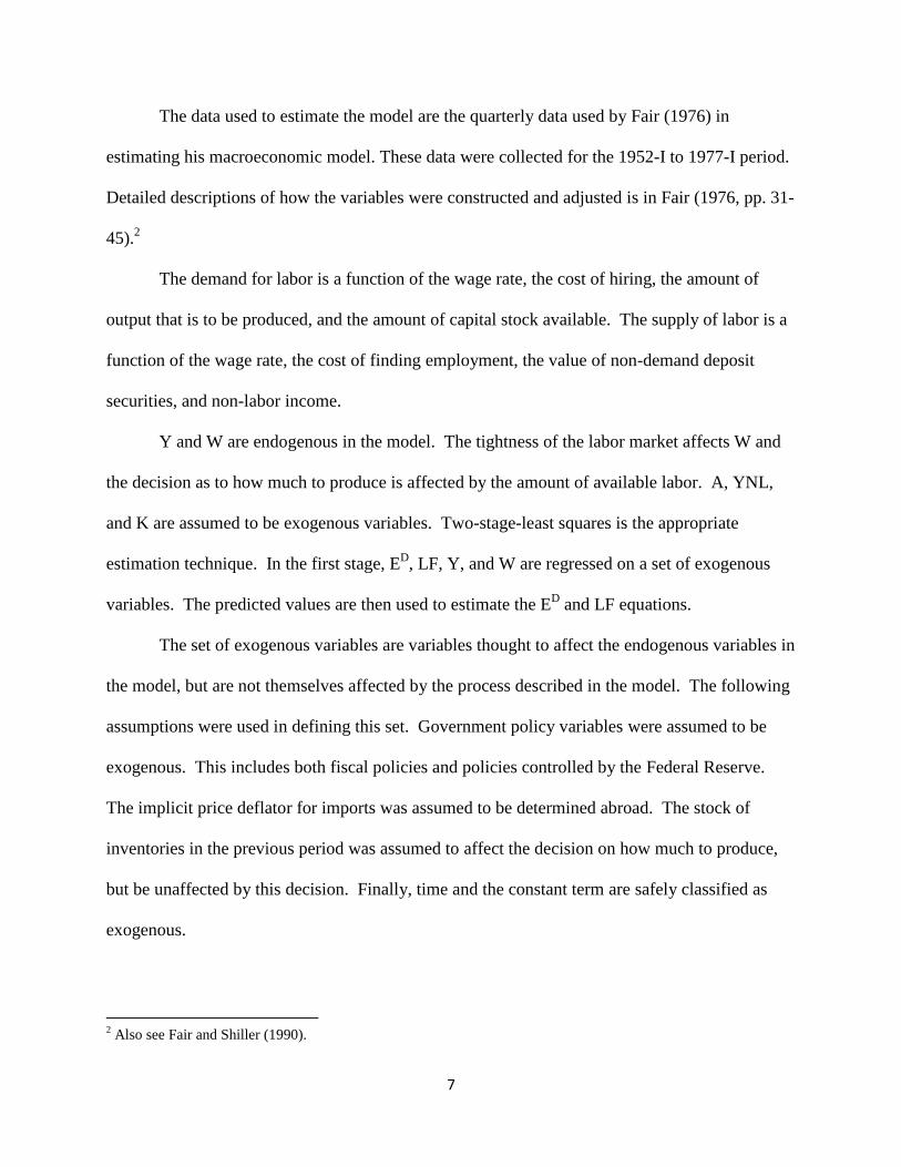
The data used to estimate the model are the quarterly data used by Fair (1976) in
estimating his macroeconomic model. These data were collected for the 1952-I to 1977-I period.
Detailed descriptions of how the variables were constructed and adjusted is in Fair (1976, pp. 31-
45).2
The demand for labor is a function of the wage rate, the cost of hiring, the amount of
output that is to be produced, and the amount of capital stock available. The supply of labor is a
function of the wage rate, the cost of finding employment, the value of non-demand deposit
securities, and non-labor income.
Y and W are endogenous in the model. The tightness of the labor market affects W and
the decision as to how much to produce is affected by the amount of available labor. A, YNL,
and K are assumed to be exogenous variables. Two-stage-least squares is the appropriate
estimation technique. In the first stage, ED, LF, Y, and W are regressed on a set of exogenous
variables. The predicted values are then used to estimate the ED and LF equations.
The set of exogenous variables are variables thought to affect the endogenous variables in
the model, but are not themselves affected by the process described in the model. The following
assumptions were used in defining this set. Government policy variables were assumed to be
exogenous. This includes both fiscal policies and policies controlled by the Federal Reserve.
The implicit price deflator for imports was assumed to be determined abroad. The stock of
inventories in the previous period was assumed to affect the decision on how much to produce,
but be unaffected by this decision. Finally, time and the constant term are safely classified as
exogenous.
2 Also see Fair and Shiller (1990).
8
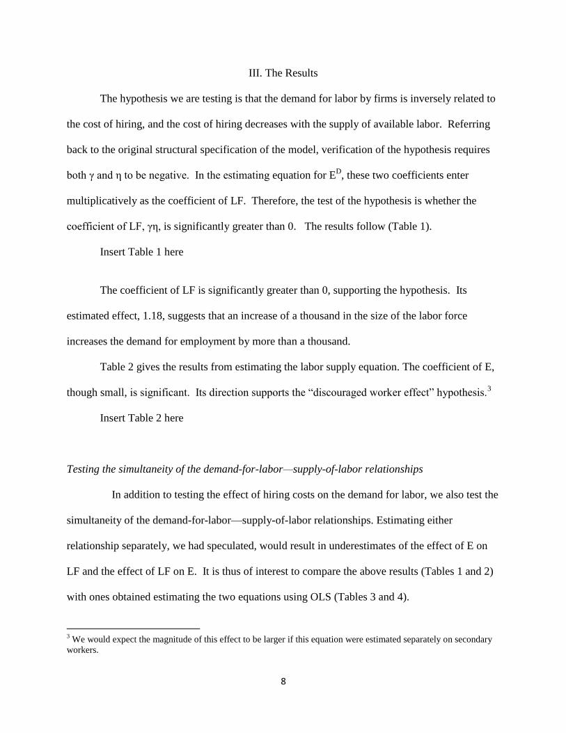
III. The Results
The hypothesis we are testing is that the demand for labor by firms is inversely related to
the cost of hiring, and the cost of hiring decreases with the supply of available labor. Referring
back to the original structural specification of the model, verification of the hypothesis requires
both γ and η to be negative. In the estimating equation for ED, these two coefficients enter
multiplicatively as the coefficient of LF. Therefore, the test of the hypothesis is whether the
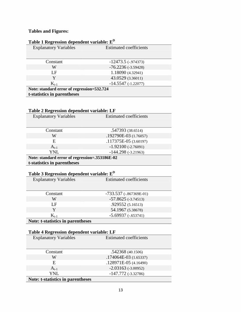
coefficient of LF, γη, is significantly greater than 0. The results follow (Table 1).
Insert Table 1 here
The coefficient of LF is significantly greater than 0, supporting the hypothesis. Its
estimated effect, 1.18, suggests that an increase of a thousand in the size of the labor force
increases the demand for employment by more than a thousand.
Table 2 gives the results from estimating the labor supply equation. The coefficient of E,
though small, is significant. Its direction supports the ―discouraged worker effect‖ hypothesis.3
Insert Table 2 here
Testing the simultaneity of the demand-for-labor—supply-of-labor relationships
In addition to testing the effect of hiring costs on the demand for labor, we also test the
simultaneity of the demand-for-labor—supply-of-labor relationships. Estimating either
relationship separately, we had speculated, would result in underestimates of the effect of E on
LF and the effect of LF on E. It is thus of interest to compare the above results (Tables 1 and 2)
with ones obtained estimating the two equations using OLS (Tables 3 and 4).
3 We would expect the magnitude of this effect to be larger if this equation were estimated separately on secondary
workers.
9
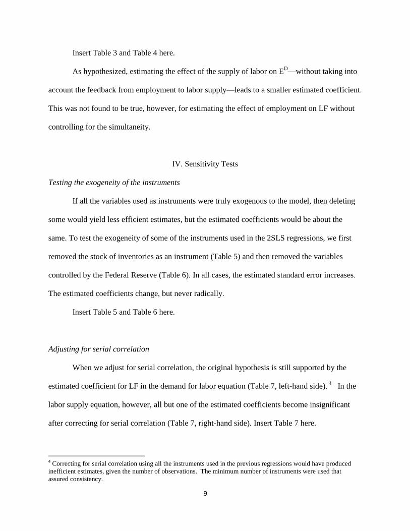
Insert Table 3 and Table 4 here.
As hypothesized, estimating the effect of the supply of labor on ED—without taking into
account the feedback from employment to labor supply—leads to a smaller estimated coefficient.
This was not found to be true, however, for estimating the effect of employment on LF without
controlling for the simultaneity.
IV. Sensitivity Tests
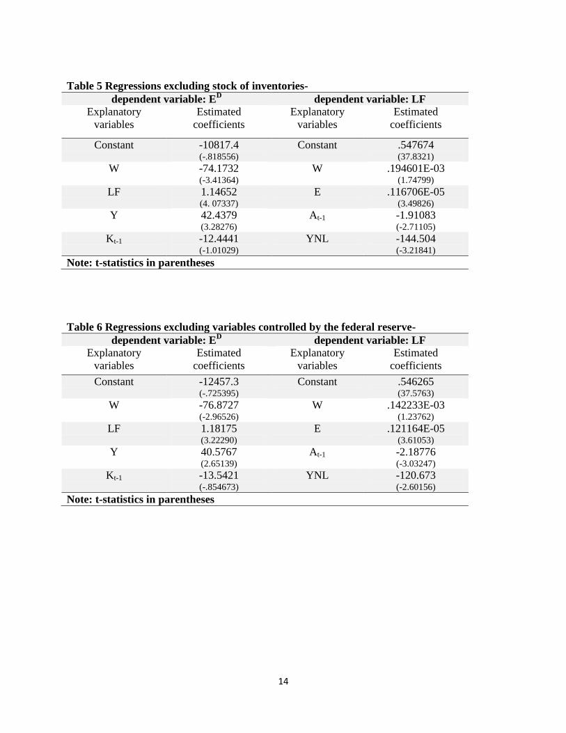
Testing the exogeneity of the instruments
If all the variables used as instruments were truly exogenous to the model, then deleting
some would yield less efficient estimates, but the estimated coefficients would be about the
same. To test the exogeneity of some of the instruments used in the 2SLS regressions, we first
removed the stock of inventories as an instrument (Table 5) and then removed the variables
controlled by the Federal Reserve (Table 6). In all cases, the estimated standard error increases.
The estimated coefficients change, but never radically.
Insert Table 5 and Table 6 here.
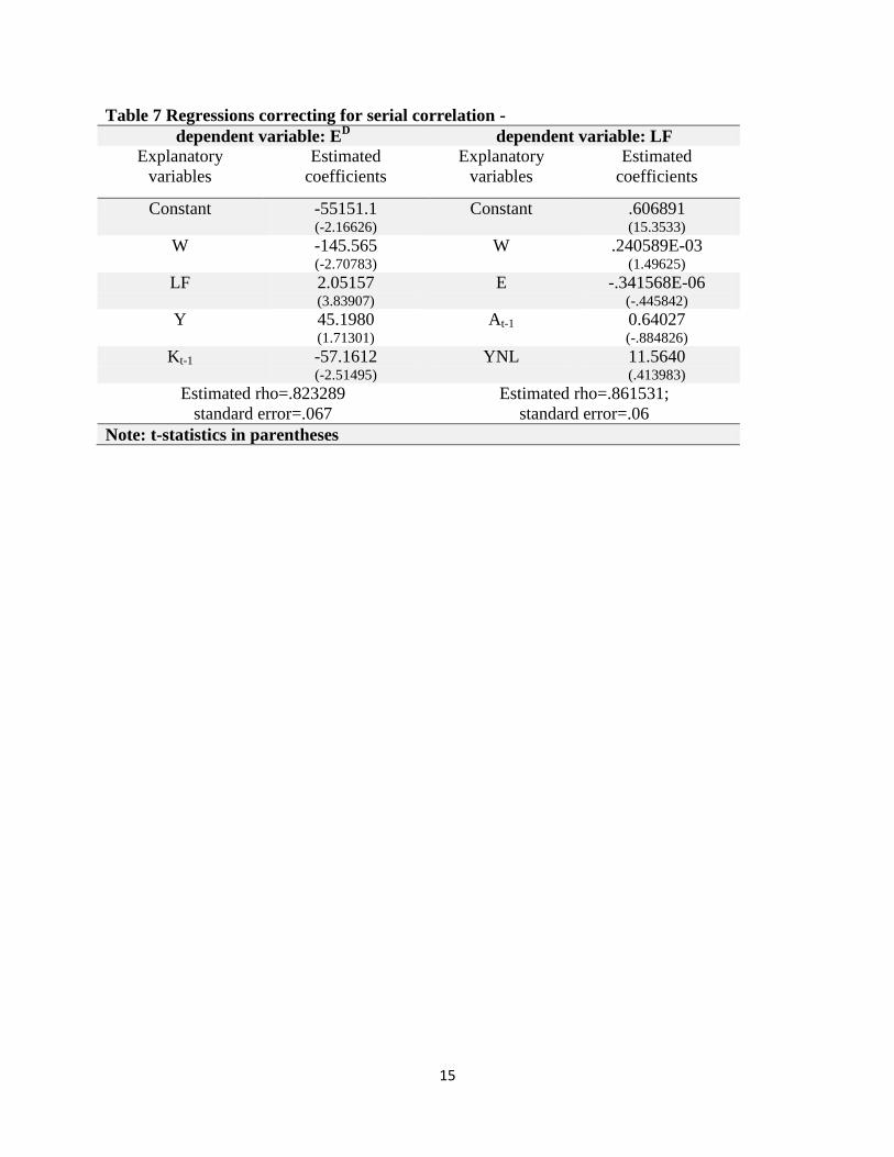
Adjusting for serial correlation
When we adjust for serial correlation, the original hypothesis is still supported by the
estimated coefficient for LF in the demand for labor equation (Table 7, left-hand side). 4
In the
labor supply equation, however, all but one of the estimated coefficients become insignificant
after correcting for serial correlation (Table 7, right-hand side). Insert Table 7 here.
4 Correcting for serial correlation using all the instruments used in the previous regressions would have produced
inefficient estimates, given the number of observations. The minimum number of instruments were used that
assured consistency.
10
V. Directions for Further Work
Evidently, one direction for further work is to lengthen, with more recent and earlier data,
the time series for estimating the model. Several steps could also be taken to more rigorously test
the model.
A truncated dependent variable
Since the demand for labor is not observed beyond a certain point, the model was
estimated only on those values for which E<.96LF. The dependent variable for the employment
demand equation is truncated. As shown in Figure 5, using only observations for which ED <
.96LF the E(ε |X) < 0 and all estimated coefficients will be inconsistent (Hausman and Wise,
1977). This is not a problem for the labor supply since the dependent variable is always
observed.
Insert Figure 5 here.
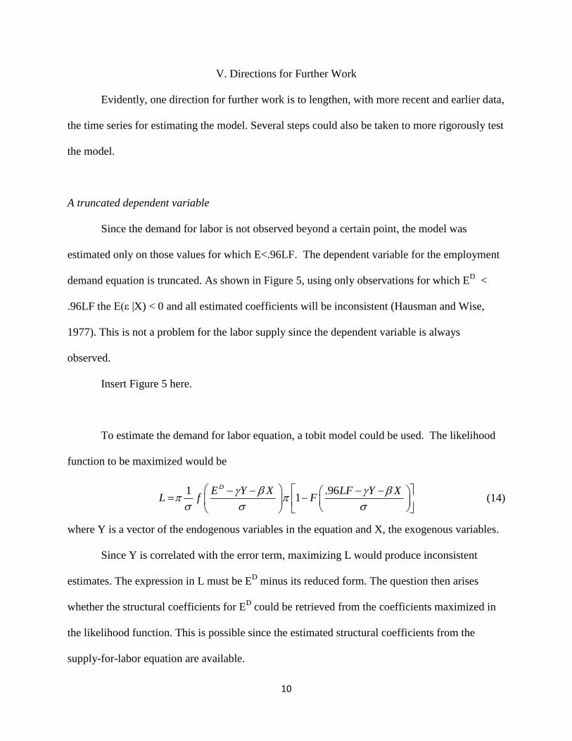
To estimate the demand for labor equation, a tobit model could be used. The likelihood
function to be maximized would be
1 .96
1 DE Y X LF Y X
L f F
(14)
where Y is a vector of the endogenous variables in the equation and X, the exogenous variables.
Since Y is correlated with the error term, maximizing L would produce inconsistent
estimates. The expression in L must be ED minus its reduced form. The question then arises
whether the structural coefficients for ED could be retrieved from the coefficients maximized in
the likelihood function. This is possible since the estimated structural coefficients from the
supply-for-labor equation are available.
11
Testing for specification error
To more rigorously test for specification error, the estimates obtained using all the
instrumental variables, ̂0, should be compared with the estimated coefficients deleting
questionable instruments, ̂. A test statistic can be formed which is distributed asymptotically
as central χ2 where K is the number of unknown parameters in β when no misspecification occurs
(Hausman, 1978).
Testing E = ED
when E<.96LF
Finally, a simple procedure could be performed to test the assumption that E = ED
when
E<.96LF.5 The demand for labor equation could be estimated on another set of observations
assuming a different truncation point, say .95LF. If the demand for employment were only
observed until E=.95LF, then the estimated coefficients would be lower for the estimated
equation assuming ED is observed until employment equals 96% of the labor force.
VI. Conclusion
Labor supply is typically viewed as a function of labor demand. This note posits a general
model of how labor demand is a function of labor supply and tests this model with historical
data. Our preliminary exploration supports an encouraged employer effect. If this conclusion
holds with more rigorous testing, two important implications follow: 1. Failure to take the
encouraged employer effect into account may help explain why a change in the labor force—
such as the addition of women or immigrants—does not increase unemployment as much as is
5 The problem of not observing the demand for employment beyond a certain point has been approached in different
contexts by investigators studying markets in disequilibrium (e.g., Fair and Jaffee, 1972; Amemiya, 1974; and
Maddala and Nelson, 1974).

12
predicted for current workers. 2. It may also explain why economists often underestimate surges
in employment.
13
Tables and Figures:
Table 1 Regression dependent variable: ED
Explanatory Variables Estimated coefficients
Constant -12473.5 (-.974373)
W -76.2236 (-3.59428)
LF 1.18090 (4.32941)
Y 43.0529 (3.36011)
Kt-1 -14.5547 (-1.22077)
Note: standard error of regression=532.724
t-statistics in parentheses
Table 2 Regression dependent variable: LF
Explanatory Variables Estimated coefficients
Constant .547393 (38.6514)
W .192790E-03 (1.76057)
E .117375E-05 (3.60197)
At-1 -1.92100 (-2.76091)
YNL -144.298 (-3.21963)
Note: standard error of regression=.353186E-02
t-statistics in parentheses
Table 3 Regression dependent variable: ED
Explanatory Variables Estimated coefficients
Constant -733.537 (-.867369E-01)
W -57.8625 (-3.74513)
LF .929552 (5.16513)
Y 54.1967 (5.38678)
Kt-1 -5.69937 (-.653741)
Note: t-statistics in parentheses
Table 4 Regression dependent variable: LF
Explanatory Variables Estimated coefficients
Constant .542368 (40.1506)
W .174064E-03 (1.65337)
E .128971E-05 (4.16490)
At-1 -2.03163 (-3.00952)
YNL -147.772 (-3.32786)
Note: t-statistics in parentheses
14
Table 5 Regressions excluding stock of inventories-
dependent variable: ED dependent variable: LF
Explanatory
variables
Estimated
coefficients
Explanatory
variables
Estimated
coefficients
Constant -10817.4 (-.818556)
Constant .547674 (37.8321)
W -74.1732 (-3.41364)
W .194601E-03 (1.74799)
LF 1.14652
(4. 07337) E .116706E-05
(3.49826) Y 42.4379
(3.28276) At-1 -1.91083
(-2.71105) Kt-1 -12.4441
(-1.01029)
YNL -144.504 (-3.21841)
Note: t-statistics in parentheses
Table 6 Regressions excluding variables controlled by the federal reserve-
dependent variable: ED dependent variable: LF
Explanatory
variables
Estimated
coefficients
Explanatory
variables
Estimated
coefficients
Constant -12457.3 (-.725395)
Constant .546265 (37.5763)
W -76.8727 (-2.96526)
W .142233E-03 (1.23762)
LF 1.18175 (3.22290)
E .121164E-05 (3.61053)
Y 40.5767 (2.65139)
At-1 -2.18776 (-3.03247)
Kt-1 -13.5421 (-.854673)
YNL -120.673 (-2.60156)
Note: t-statistics in parentheses
15
Table 7 Regressions correcting for serial correlation -
dependent variable: ED dependent variable: LF
Explanatory
variables
Estimated
coefficients
Explanatory
variables
Estimated
coefficients
Constant -55151.1 (-2.16626)
Constant .606891 (15.3533)
W -145.565 (-2.70783)
W .240589E-03 (1.49625)
LF 2.05157 (3.83907)
E -.341568E-06 (-.445842)
Y 45.1980 (1.71301)
At-1 0.64027 (-.884826)
Kt-1 -57.1612 (-2.51495)
YNL 11.5640 (.413983)
Estimated rho=.823289
standard error=.067
Estimated rho=.861531;
standard error=.06
Note: t-statistics in parentheses
16
Figure: Historical time series of U.S. employment and the labor force
0
50000
100000
150000
200000
250000
300000
19
49
19
52
19
55
19
58
19
61
19
64
19
67
19
70
19
73
19
76
19
79
19
82
19
85
19
88
19
91
19
94
19
97
20
00
20
03
20
06
20
09
20
12
tho
usa
nd
s in
div
idu
al
U.S. Labor force and employment trends 1949 - 2013
civillian population
Labor force
Employment
17
18
19
References
Amemiya, T (1974). ―A Note on a Fair and Jaffee Model,‖ Econometrica, 42(4): 759- 762.
Fair, Ray C. (1976) Model of Macroeconomic Activity: The Empirical Model v. 2 Ballinger
Publishing Co.
Fair, Ray C. and Dwight M. Jaffee, (1972) ―Methods of Estimation for Markets in
Disequilibrium,‖ Econometrica, 40(3):497-514.
Fair, Ray C. and Robert J. Shiller. (1990). ―Comparing Information in Forecasts from
Econometric Models,‖ American Economic Review, 80(3):175-189.
Hausman, Jerry A. (1978). ―Specification Tests in Econometrics,‖ Econometrica, 46(6): 1251–
1271.
Hausman, Jerry A. and David A. Wise, (1977). ―Social Experimentation, Truncated Distributions
and Efficient Estimation,‖ Econometrica, 45(4), 319-39.
Maddala, G. S. and Forest D. Nelson, ―Maximum Likelihood Methods for Models of Markets in
Disequilibrium,‖ Econometrica, 42(6), 1013-1030.