Embed Size (px)
Citation preview

How should we measure the fear of job loss?
by Andy Dickerson* and Francis GREEN**
Paper prepared for Fifth IZA/SOLE Transatlantic Meeting of Labour Economists, 18-21 May 2006; Buch-Ammersee, Germany.
* Institute for Employment Research, University of Warwick.
** University of Kent.
Address for Correspondence:
Francis Green, Professor of Economics, Department of Economics, Keynes College, University of Kent, Canterbury CT2 7NP, UK. [email protected] Tel: 44 1227 827305 http://www.kent.ac.uk/economics/staff/gfg/

ABSTRACT
We investigate the value of subjective data on expectations of job loss, primarily by examining the associations between expectations and realisations, among representative samples of German and Australian workers taken, respectively, from the German Socio-Economic Panel (GSOEP) and from the Household Income and Labour Dynamics in Australia Survey (HILDA) . We find that:
a. Collection of subjective expectations data on job loss is worthwhile because the data reveal private information on job loss risk, as shown both with the raw data and using conventional panel estimators.
b. On average, workers in both countries over-estimate the chance of losing their job by a factor of approximately two.
c. Cardinal probability scales show a non-linear relationship between expectations and realisations.
d. As predictors of subsequent job loss, expectations of job loss data did not perform clearly better after the GSOEP scale switched from ordinal verbal descriptors to cardinal numerical descriptors in 1999.
e. In a small minority of cases responses to cardinal scales showed inconsistencies with other expectations data.
f. No great inter-group differences were found for the extent to which workers over-estimated their chances of job loss.
We recommend that, when framing questions on expectations of job loss, researchers should:
i) Be explicit and unambiguous about the risk under investigation; in general focus on the single event of job loss rather than conflating this with other elements of insecurity.
ii) Utilise an ordinal scale, with relatively few scale points.
iii) Devise unambiguous descriptors for every scale point. One possible strategy is to use probability ranges.

1. Introduction. Perceptions of job insecurity have been found to generate anxiety and lower the well-being of workers and their dependents, to inhibit consumer spending, and to reduce the wage growth of male employees (Wichert, 2002; Benito, 2004; Lusardi, 1998; Carroll et al., 2003; Campbell et al., forthcoming 2007). In addition to such practical effects, job insecurity perceptions have also been to some extent validated in two recent studies, one for a sample of older Canadian men, the other using two nationally representative samples of British workers of all ages. These studies give evidence that job loss risk perceptions are correlated with subsequent experiences of job loss, but that employees are nevertheless pessimistic, in that many overestimate the chances of losing their job. Unsurprisingly, job insecurity perceptions tend to track labour market tightness; they also fit a plausible model of how expectations are formed, reflecting objective labour market factors, prior unemployment experiences and other social encounters with unemployment (Schmidt, 1999; Green et al., 2000; Manski and Straub, 2000; Campbell et al., forthcoming 2007; Stephens, 2004).
Because of its welfare-reducing effects it is natural to look for ways of reducing insecurity perceptions. Macroeconomic stabilisation policies serve this function, but in addition Bryson et al. (2004) find that firm-level job protection policies do have the desired effect of reducing employees’ feelings of insecurity. Clark and Postel-Vinay (2004), however, find that the presence of economy-wide employment protection laws is associated with raised insecurity perceptions. A possible reason for this apparently perverse finding is that respondents may have interpreted the job security instrument from the European Community Household Panel utilised in that study to include the cost of job loss. As Clark and Postel-Vinay note, if employment protection is associated with longer unemployment spells, the protection laws raise the cost of job loss, and this effect may outweigh any downward impact on the risk of job loss. This confounding of two components of job insecurity is one illustration of a problem throughout much of the literature on job security, namely that there lacks sufficient clarity and consistency across studies in the way that job insecurity is conceived and measured (Green, 2006). Job security comprises multiple parts: the expectation of job loss, its potential cost, and the uncertainty surrounding future wages if the job continues. Survey questions about job insecurity are sometimes imprecise1, and the responses may be affected by all three elements in unknown proportions. Questions about satisfaction with security introduce the further dimension of how much security the employee was counting on in the first place.
The best research practice is to develop where possible instruments that measure validly and reliably the separate components of insecurity. The aim of this paper is therefore to contribute some evidence about the methodology of measuring job insecurity, with a view to informing instrument design in future research. We focus on the first component, the expectation of job loss.2 Recent papers have examined and supported the usefulness of subjective expectations data in economics generally (Hurd and McGarry, 2002; Manski, 2004). We add to the case that expectations of job loss can be effectively measured through direct survey instruments. We extend the finding of conditional correlation between job loss risk perception and subsequent job loss for Canada and Britain to two more countries, namely Germany and Australia. In the Canadian and British studies noted above, it was possible that this correlation could have been due to unobserved individual heterogeneity, whereby individuals with an undisclosed propensity to worry are selected into low quality and more insecure jobs. In this 1 For example, the question in the International Social Survey Programme of 1989 and 1997 asks for the extent of agreement/disagreement with the statement: “My job is secure”. 2 There is a separate literature on estimates of the cost of job loss and its change over time - see Green (2006) for a review.
1
paper, we exploit longitudinal data to account for that possibility. Our findings for both countries strengthen confidence in the conclusion that expectations can predict subsequent job loss.
Additionally it turns out that German and Australian workers also show pessimism in their job loss expectations. We investigate whether this pessimism is a statistical artefact resulting from strategic quitting to pre-empt redundancy; or, equally mundanely, a mis-timing of the prediction whereby job loss does come about as predicted, but occurs later than had been anticipated.
An important methodological issue is the choice of response scale for questions on the risk of job loss. A cardinal scale, in which respondents are asked to state the probability of job loss, has considerable attraction if respondents can sensibly and reliably answer on such a scale. With a probabilistic scale, interpersonal and intra-personal comparisons of perceptions can also be scaled. Use of non-probabilistic scales with verbal descriptors relies on assuming that respondents have a shared understanding of the descriptors, and restricts comparisons to ordinal rankings. Yet while some small-scale studies in psychology imply that it is possible to elicit probabilistic expectations in certain domains, we lack evidence as to whether such replies are reliable, or whether they contain more information than ordinal scales. We provide some tests of the feasibility and reliability of a cardinal probability scale, using large representative samples of employees in Germany and Australia, and compare the predictive power of a cardinal scale with that of an ordinal scale. Finally, we examine whether expectations of job loss are more accurate, as might be expected, for groups that are better informed or more educated.
The paper proceeds as follows. The next section reviews arguments and existing evidence concerning the use of probabilistic or ordinal scales when measuring expectations, and reviews possible explanations for the pessimism shown in the previous studies. Section 3 describes the data. The main findings which address the research questions posed above are presented in Section 4, 5 and 6. Finally, Section 7 concludes with a discussion of the implications for the construction of questions on the expectations of job loss.
2. Issues in the Measurement of the Risk of Job Loss
Manski (2004) makes a powerful argument for economists to directly measure expectations of future events. Rather than assuming an ideal process of expectations formation (usually ‘rational’) and then identifying decision processes from observed behaviour, Manski advocates combining choice data with self-reported data on perceived expectations. He suggests that this should ‘mitigate the credibility problem’ associated with defending unrealistic maintained assumptions about expectations formation. His paper then surveys an emerging literature on the feasibility, method and reliability of measuring expectations in diverse fields including the return to schooling, job loss risk, cost of job loss, fertility, consumer spending, survival time, and social security.
One problem in some of the literature is that respondents are sometimes presented with too few alternative responses – for example, will ‘x’ happen, yes or no. An obvious recommendation is that respondents be allowed to reported the perceived likelihood of x happening.
But how might respondents report that likelihood? A common procedure is to use an ordinal verbal scale such as “no chance”, “very unlikely”, “unlikely”, “evens”, “quite likely”, “very likely”. Yet it is possible that these descriptors are not interpersonally comparable, if different individuals do not have a shared understanding of the descriptors. An alternative procedure is
2

to use a probabilistic scale. A cardinal ranking would mitigate the problem of interpersonal comparisons because the meaning of any given percentage should be identical for all (numerate) respondents. Moreover, a cardinal measure of risk is potentially more efficient or parsimonious as an explanatory variable in econometric analyses. Manski (2004) cites evidence that respondents are willing to make probabilistic judgements, and finds no indication of internal inconsistencies in these cases. The counter-argument is the assertion that respondents may not be capable of making reliable cardinal probability judgements. Even though they are willing to report subjective cardinalprobabilities, these may not correspond with objective circumstances. Lukasiewicz et al. (2001) note the paucity of work validating scales of risk perception, and provide some evidence in favour of using verbal scales for measuring instantaneous perceptions of risk. Erev and Cohen (1990) report experimental evidence that verbal and numerical scales were equally efficient at conveying event probabilities, and that judgemental biases (wishful thinking and/or the conjunction fallacy) occurred independently of which kind of scale was used.
One issue to be investigated in this paper, therefore, is whether cardinal scales for questions on job loss expectations perform better, in the sense of achieving greater reliability than ordinal scales while maintaining face validity. An adjunct to this question concerns how to phrase the probabilistic scale. Options are to ask respondents to report any integer from 0 to 100, to present single points on a coarser scale (e.g. 0 to 10), or to present banded ranges for the probability. To assess the reliability of subjective expectations data one cannot directly check whether the respondents really do hold the expectations they report, since it is normally infeasible to directly measure neural processes that accompany the answering of questions. Rather, one can instead check to what extent the reported expectations are realised, as well as whether they conform to a plausible model of expectations formation. In this paper we confine ourselves to evidence on realisations, this being the more stringent test.
Two aspects of these realisations are of interest, corresponding to the marginal and the average expectation. We shall say that the marginal expectation is reliable to the extent that an incremental rise in the perceived probability of job loss is matched by an equal rise in the frequency of job loss. Second, a reliable predictor for a group will be realised on average across all in the group. If the average perceived probability of job loss is greater than the average outturn, that group is said to suffer from pessimism on average. Systematic average optimism or pessimism has been found in a number of fields. Smokers, for example, typically suffer from unrealistic optimism. They underestimate their chances of contracting lung cancer, an error that is usually attributed to information deficit (e.g. Weinstein et al., 2005). Similarly, drivers and motorbike riders under-estimate the chances of having an accident (e.g. Rutter et al., 1998). A prominent explanation is that drivers may suffer from an illusion of control. In other fields pessimism is found, for example with respect to air travel. One source of pessimism in the case of negative risk is said to be an individual’s propensity to worry, since it is maintained that worriers are more likely than others to rehearse the reasons why negative events could happen (Constans, 2001). While there is no comprehensive psychological account of pessimism, a useful point of this literature is that accuracy of predictions is likely to be related to the amount of information available to respondents, and their ability to process it.
Concerning the risk of job loss the main finding in the cases of both Canada and Britain (Stephens, 2004; Campbell et al., forthcoming 2007) is that employees are pessimistic about job loss, in that they overestimate the chances of job loss both at the margin and on average. In this paper we investigate whether pessimism about job loss is a more general phenomenon, and whether pessimism is found whatever scale is used, cardinal or ordinal.
3

3. Data To investigate these issues we make use of two panel data sets, the German Socio-Economic Panel (GSOEP), which runs from 1984 to the present, and the Household Income and Labour Dynamics in Australia (HILDA) Survey which began in 2001.
GSOEP is a panel survey of households in Germany, including, from 1990 onwards, East Germany. The first wave in 1984 comprised 12,290 individuals in 5,921 households; the sample is depleted annually with some attrition, and replenished with regular additions through household splitting and expansion, and through occasional refreshment. Full details are given at the website: http://www.diw.de/english/sop/. 3
Regularly, though not every year, respondents are asked about their expectations in the labour market. Respondents in employment are asked: “How probable is it in the next two years that you will lose your job?”, and the question is posed with the same words every time. Other expectations are also enquired about, for example retirement and promotion possibilities, though the range of these varies across waves. The response scale to all the expectations questions was, for the years 1985, 1987, 1989, 1991, 1993, 1994, 1996 and 1998, a consistent ordinal scale with descriptors: “definitely”, “probably”, “probably not”, “definitely not”.4 In 1999, 2001 and 2003, while the question on the expectation of job loss remained the same as in earlier years, the response scale was cardinal. Respondents were asked to indicate the likelihood of the event happening by answering on a scale labelled 0, 10, 20 … to 100, where “the value 0 means that it is certain not to take place” and “the value 100 means that it is certain to take place”. The switch from an ordinal to a cardinal scale enables us to carry out a “before-after” test of the predictive powers of the two scales. For the purposes of this paper, we focused on the 1994, 1996 and 1998 waves, from before the scale switch, and all relevant waves after the scale switch currently available (to be updated), namely 1999, 2001 and 2003.
Also required is an indication for whether job loss is realised in the period subsequent to the expectation being expressed. Job loss here is defined as a job termination due to dismissal, a temporary job or apprenticeship being completed or the close of the business (including for self-employed people). Dismissal is the most frequent of these three reasons. Note that job loss does not necessarily imply a period of unemployment. For the expectation expressed in year t, we have taken the relevant 2-year period to be during year t or year t+1.5
HILDA is a panel survey of Australian households. The first wave was drawn from a probability sample, and comprised 7,682 household interviews, with a response rate of 66%. Within households, 92% of eligible (aged over 15) persons responded, giving 13,969 individuals. The questionnaires investigate labour market dynamics, family dynamics, and economic and subjective well-being. Full details of the panel, including subsequent attrition rates and sample renewal procedures, are given in the HILDA Users Manual available from http://melbourneinstitute.com/hilda/.
3 The data was made available to us by the German Socio-Economic Panel Study (SOEP) at the German Institute for Economic Research (DIW Berlin). 4 The English version translation was different before 1998, but the German scale remained unaltered; the translation given here, used for 1998, is most accurate. 5 Most interviews (between two-thirds and three-quarters) are completed by the end of March in each year, so this does not seem unreasonable. We will test the sensitivity to this assumption later using the calendar data present in GSOEP in ongoing work, but do not anticipate that this will alter our findings substantially. Note that realisations following the 2003 expectations are absent until the 2005 wave becomes available.
4

Each year the HILDA survey asks a number of questions about the labour market expectations of respondents, and for those in employment these questions focus on expectations of job loss, of (voluntary) quitting, and of getting another equally good job in the event of job loss. We restricted our sample to those who were employees when they express their expectations of job loss. The question on risk of job loss is: “I would like you to think about your employment prospects over the next 12 months. What do you think is the per cent chance that you will lose your job during the next 12 months? By loss of job, I mean getting fired, being laid off or retrenched, being made redundant, or having your contract not renewed.” This question is excellent, as its meaning is clear and unambiguous: each respondent can be expected to have the same understanding of the question (in particular, about what is meant by “loss of job”) as other respondents and researchers.
The issue here then revolves around the response scale. The respondents simply give a number anywhere between 0 and 100 inclusive. There would appear to be no validity doubts here; the only issue is whether respondents can answer reliably about their objective situation.
In Waves 2 onwards, some questions address recent employment and unemployment experiences, and in particular respondents are asked to give the main reason why the job that they held at the previous interview had ceased. We collapsed the multiple reasons into two types, according to whether they had ceased working in the job voluntarily, or whether this had been involuntary. The latter included: dismissal, employer out of business, laid off, made redundant, no work available, retrenched, temporary or seasonal job.
Both GSOEP and HILDA also collect a rich array of variables, some of which we used as controls in our analysis of job loss: highest education, age, gender, contractual status, recent unemployment experience, sector and establishment size.
4. Findings
a) Distribution of Responses
A basic requirement for any question on the expectation of job loss is that respondents take sufficient meaning from the question and the response scale to be able to answer it. Re-assurance is immediately forthcoming for the instruments used in both GSOEP and HILDA. For GSOEP, the proportion of respondents unwilling or unable to answer the question was 1.56% and 1.25% in the period before and after the change in the scale respectively. For HILDA, there were only 0.1% missing responses. Respondents are thus willing to report expectations against either ordinal or cardinal scales. Possibly, the very low figure for HILDA is a reflection of its unambiguous question wording.
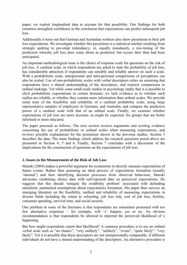
A second requirement for a good instrument is that the distribution of responses should be spread across scale response points in a plausible way. Figures 1 to 3 present these responses (averaged over years) for GSOEP (ordinal), GSOEP (cardinal) and HILDA.
As can be seen from all three figures, the large majority do not expect to lose their job. In the GSOEP (ordinal) period (Figure 1), about one in ten perceived that job loss was probable or definite in the following two years, while 31% said that they would definitely not lose their job. In the ensuing GSOEP (cardinal) period, the proportion answering that the chance of job loss was zero was 42.5%. The difference from the immediately preceding years using the ordinal scale suggests that some respondents replying “improbable” are induced to reply zero when presented with a cardinal scale. Figure 2 gives the distribution for all those not replying zero. As can be seen, even though respondents are constrained to reply at decile points, there are apparent spikes at both 50% and 100%.
5
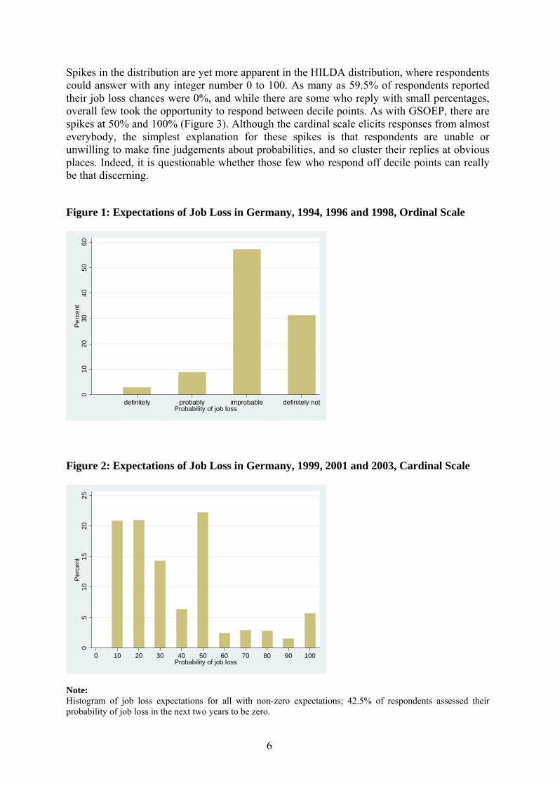
Spikes in the distribution are yet more apparent in the HILDA distribution, where respondents could answer with any integer number 0 to 100. As many as 59.5% of respondents reported their job loss chances were 0%, and while there are some who reply with small percentages, overall few took the opportunity to respond between decile points. As with GSOEP, there are spikes at 50% and 100% (Figure 3). Although the cardinal scale elicits responses from almost everybody, the simplest explanation for these spikes is that respondents are unable or unwilling to make fine judgements about probabilities, and so cluster their replies at obvious places. Indeed, it is questionable whether those few who respond off decile points can really be that discerning.
Figure 1: Expectations of Job Loss in Germany, 1994, 1996 and 1998, Ordinal Scale
010
2030
4050
60P
erce
nt
definitely probably improbable definitely notProbability of job loss
Figure 2: Expectations of Job Loss in Germany, 1999, 2001 and 2003, Cardinal Scale
05
1015
2025
Per
cent
0 10 20 30 40 50 60 70 80 90 100Probability of job loss
Note: Histogram of job loss expectations for all with non-zero expectations; 42.5% of respondents assessed their probability of job loss in the next two years to be zero.
6

Figure 3: Expectations of Job Loss in Australia, 2000-2004, Cardinal Scale
05
1015
2025
Per
cent
0 5 10 15 20 25 30 35 40 45 50 55 60 65 70 75 80 85 90 95 100Probability of job loss
Note: Histogram of job loss expectations for all with non-zero expectations; 59.5% of respondents assessed their probability of job loss in the next year to be zero. b) Perceptions and Realisations of Job Loss
Next we investigate how closely respondents’ expectations of job loss match the realisations of job loss. Tables 1 and 2 show this match for Germany and Australia respectively. We group respondents according to their perceptions of the risk of job loss – at their precise decile scale points for Germany, and in decile bands for Australia.
As can be seen, on average respondents in both Germany and Australia tend to overestimate the risk of job loss by a factor of approximately two. In Germany, the mean perceived probability of 2-year job loss in 1999 and 2001 was 20.5%, but the average realised incidence of job loss in the subsequent two years was 9.5%. Corresponding figures for the 1-year risk in Australia over 2001-2003 were 11.5% and 5.7%.
In fact, in both countries, the cardinal scales indicate that overestimation of risk occurs for all groups that envisage a non-zero risk of job loss. In contrast, those who report that there is no chance of losing their job are underestimating the risk to a small extent: for them, the incidence of job loss was 5.4% in Germany, and 3.5% in Australia.
The verbal ordinal scales also indicate overestimation of risk in Germany for those who perceive some risk: among those in the “definitely” category, the incidence of job loss was only 42%. This amount is quite close to the job loss incidence (46%) found for those answering 100% on the cardinal scale. Similarly, underestimation occurs at the no-risk end of the scale: job loss incidence was 4% among those in the “definitely not” category.
Despite this overestimation on average, there is a positive relationship between perceived job loss band and the subsequent incidence of job loss. In the case of Germany this relationship is monotonic, and for Australia it is nearly so. With few exceptions, being in a group that expects a higher chance of job loss is indeed linked with a higher incidence of job loss. We
7

take this finding as confirming that responses do convey useful information about employment prospects.
Figure 4 shows that the relationships between perception and realisation in Germany and Australia are quite similar. The 45o line denotes perfect prediction – that is when outcomes are the same as perceptions. In both countries the line runs below the 45o line for most of its length. It is also sloped less steeply. Both the finding of the presence of overestimation (together with underestimation at the no-risk end of the scale), and the finding of a monotonic (or near-monotonic) relationship between perception and realisation, make the pattern of responses from Germany and Australia similar to those in Britain and Canada.
Finally, note that the relationships shown in Figure 4 are non-linear at the top end of the scale in both countries. Stephens (2004) finds something similar for his sample of older Canadian men. This finding implies a shortcoming of the cardinal scale, since such a scale assumes that the marginal change in the probability of job loss is measured by changes in the number reported for the perceived probability. Yet it transpires that in Germany a change in perception from, say, 20% to 30% is matched by a 3 percentage point increase in the incidence of job loss; but a change from 90% to 100% is matched by a 22 percentage point increase in incidence of job loss. The same pattern of non-linearity holds for Australia, and in addition there is a break in the monotonic relationship around some off-spike points of the distribution.
It is possible that the observed overestimation could be due to strategic quitting, whereby those expecting to lose their job pre-empt this event by quitting voluntarily. If large numbers of respondents were doing this, the “true” proportion losing their job might come close to that expected. However, at least in the case of Australia this is not the case. Employees’ quit rates are placed alongside the job loss groups in Table 2. Overall, about one in six employees quit in any year. As can be seen, there is only a weak relationship between job loss expectation and quitting. Another possibility is that many respondents were right to expect job loss, but were wrong in their estimation of how imminent it was. If the job loss were expected in one year but came, instead, within two years, the realisation of expectations might be seen as less far out. However, as Table 2 shows, again this possibility does not materialise: the job loss in the second year is not positively related to the bands for probability of job loss in one year. We thus conclude that overestimation of job loss is a genuine phenomenon.
8

Table 1: Proportions of Employees Losing Their Job by Perceived Likelihood of Job Loss in Germany1
Ordinal/category scale (1994, 1996 and 1998)
Cardinal/numerical scale2 (1999 and 2001)
Actual Job Loss Actual Job Loss Perceived likelihood of job loss: 1 (%) (s.e.)
Perceived likelihood of job loss: 1 (%) (s.e.)
Definitely Not 4.0 (0.2) 0% 5.4 (0.2) Probably Not 7.6 (0.2) 10% 5.7 (0.5) Probably 23.0 (0.9) 20% 6.7 (0.5) Definitely 42.4 (2.0) 30% 9.5 (0.7) 40% 11.6 (1.2) 50% 15.8 (0.8) 60% 18.0 (2.5) 70% 19.9 (2.4) 80% 20.7 (2.5) 90% 24.3 (3.6) 100% 46.1 (1.9)
Notes: 1. Time frame for perceived likelihood of job loss question and actual job loss experienced is
two years for both ordinal (category) and cardinal (numerical) scales. 2. Respondents give the perceived likelihood of job loss on a discrete 0 to 100 scale at decile
intervals, and are told that 0 means certain not to happen, while 100 means certain to happen.
3. Standard errors (s.e.) are in parentheses. Ordinal scale (1994, 1996 and 1998): Mean (s.e.) proportion experiencing job loss: 0.088 (0.002) Number of observations: 22,507 Cardinal scale (1999 and 2001): Mean (s.e.) proportion experiencing job loss: 0.095 (0.002) Mean (s.e.) perceived likelihood of job loss: 0.205 (0.002) Number of observations: 19,747
9
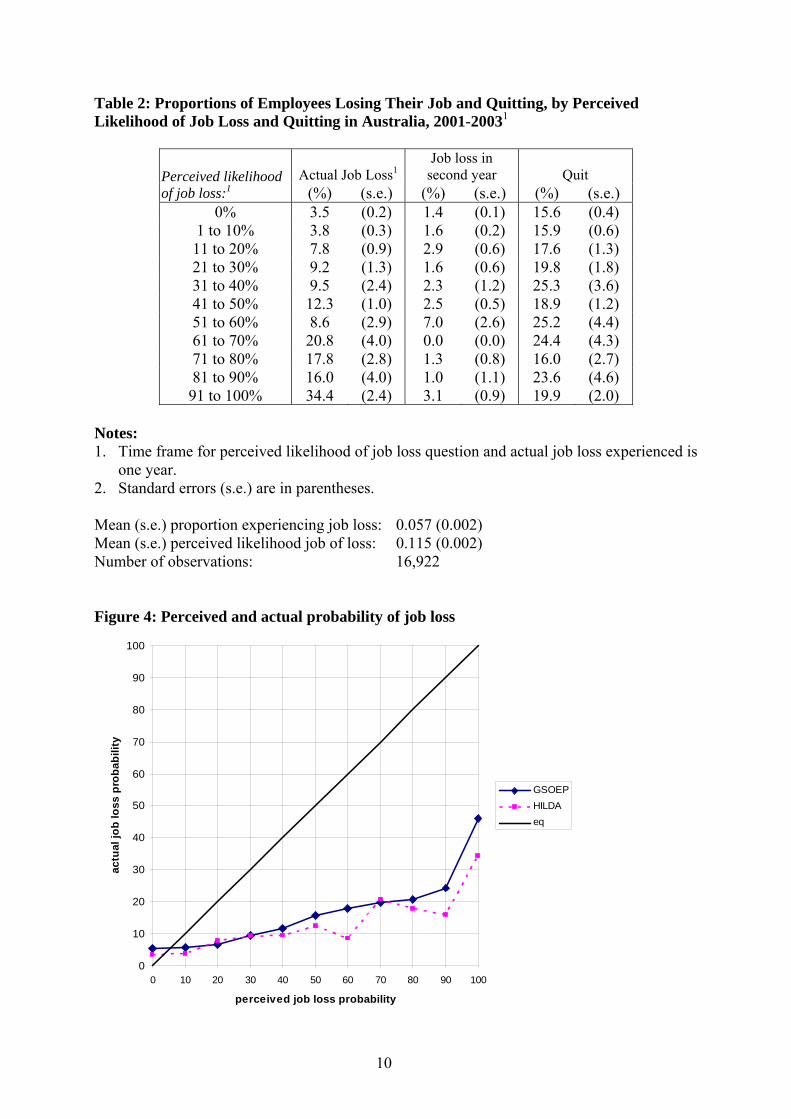
Table 2: Proportions of Employees Losing Their Job and Quitting, by Perceived Likelihood of Job Loss and Quitting in Australia, 2001-20031
Actual Job Loss1Job loss in
second year Quit Perceived likelihood of job loss:1 (%) (s.e.) (%) (s.e.) (%) (s.e.)
0% 3.5 (0.2) 1.4 (0.1) 15.6 (0.4) 1 to 10% 3.8 (0.3) 1.6 (0.2) 15.9 (0.6) 11 to 20% 7.8 (0.9) 2.9 (0.6) 17.6 (1.3) 21 to 30% 9.2 (1.3) 1.6 (0.6) 19.8 (1.8) 31 to 40% 9.5 (2.4) 2.3 (1.2) 25.3 (3.6) 41 to 50% 12.3 (1.0) 2.5 (0.5) 18.9 (1.2) 51 to 60% 8.6 (2.9) 7.0 (2.6) 25.2 (4.4) 61 to 70% 20.8 (4.0) 0.0 (0.0) 24.4 (4.3) 71 to 80% 17.8 (2.8) 1.3 (0.8) 16.0 (2.7) 81 to 90% 16.0 (4.0) 1.0 (1.1) 23.6 (4.6) 91 to 100% 34.4 (2.4) 3.1 (0.9) 19.9 (2.0)
Notes: 1. Time frame for perceived likelihood of job loss question and actual job loss experienced is
one year. 2. Standard errors (s.e.) are in parentheses. Mean (s.e.) proportion experiencing job loss: 0.057 (0.002) Mean (s.e.) perceived likelihood job of loss: 0.115 (0.002) Number of observations: 16,922 Figure 4: Perceived and actual probability of job loss
0
10
20
30
40
50
60
70
80
90
100
0 10 20 30 40 50 60 70 80 90 100
perceived job loss probability
actu
al jo
b lo
ss p
roba
bilit
y
GSOEPHILDAeq
10

c) Predicting job loss
We now turn to examine the degree to which individuals’ perceptions of the probability of job loss are useful predictors of subsequent job loss outcomes. Tables 3 and 4 contain the findings for Germany for the ordinal and cardinal perceptions of job loss scales respectively, while Table 5 reports the results for Australia. Given the binary nature of the dependent variable (‘job loss’), logit regression coefficients are reported in all cases.
In Table 3, individuals’ responses using the ordinal response scale for the fear of job loss recorded in 1994, 1996 and 1998 are correlated with the actual job loss outturns over the subsequent two years. The omitted category of individuals’ perceptions of job loss is ‘Definitely not’. Three different estimators are presented in columns (1), (2) and (3) – pooled logit, random effects logit and (conditional) fixed effects logit estimates respectively. Columns (4), (5) and (6) include a number of additional control variables which may also impact upon individuals’ probability of losing their job. These are gender, a quadratic in age, whether the individual is a graduate (or equivalent), whether they work in the private sector, or in a large establishment and, finally, whether they have had an unemployment spell in the previous year.
As can be seen from column (1), individuals’ fear of job loss is strongly and significantly correlated with their subsequent job loss propensity. The strongly monotonic increasing relationship between perceptions of job loss and job loss probability seen in the raw data in Table 1 is replicated in these logit estimates. This finding is consistent with those in Campbell et al. (forthcoming, 2007) for the UK and Stephens (2004) for Canada. It is also evident in column (2) where the random effects specification takes into account the fact that there are repeated observations on the same individuals. In both Campbell et al (forthcoming, 2007) and Stephens (2004), and in Columns (1) and (2) of Table 3, it remains possible that unobserved factors are affecting both the incidence of job loss, and the perceptions of the risk of job loss. If that were the case, the estimated coefficients would be biased, so one could not be sure that the perceptions themselves were predicting the future outcomes. One way to mitigate this problem is to estimate a (conditional) fixed effects logit, as reported in Column (3). The coefficient estimates are somewhat reduced,6 compared to those in Columns (1) or (2), but nevertheless remain highly significant and monotonically increasing across the ordinally ranked scale point descriptors.
A further step is to condition explicitly for other observable predictors of job loss. Columns (4) presents pooled logit estimates including the control variables. The coefficients on these control variables indicate that women are less likely to lose their jobs while the relationship between job loss and age shows a U-shape, with the probability declining until about age 45 years, and then increasing again. Individuals who are more highly educated, work in the public sector and/or in large establishments are all less likely to lose their jobs. Finally, those who have been unemployed in the last year are more likely to lose their job once more, usually attributable to scarring. However, despite the inclusion of these statistically significant determinants of the probability of job loss, the perceived probability of job loss continues to
6 Strictly speaking, the coefficients in the separate columns (1) to (6) cannot be directly compared without a normalisation to take account of the fact that the variance of the underlying latent variable will be different between the columns, and this will in turn affect the magnitudes of the estimated coefficients (Long, 1997, Winship and Mare, 1984). However, the difference in variance is very marginal, for either with and without control variables, and before and after the change from the ordinal to the cardinal scale as presented in Table 4. Hence we do not implement this normalisation here.
11

be a statistically significant determinant of job loss outcomes. Indeed, the coefficients are little changed from the specifications which do not include these controls. The same is true for columns (5) and (6) which present the random effects logit and (conditional) fixed effects logit estimates including controls.7 Thus the perceptions data do appear to contain private information about job loss risk that is not revealed by observed conventional indicators of job loss risk.
Tables 4a and 5a, for Germany and Australia respectively, have a similar format to Table 3, with the sole difference that they report the results obtained using the cardinal scale responses for the fear of job loss. Once again, individuals’ perceptions of their likelihood of losing their job are strongly and significantly correlated with the probability that they actually do subsequently lose their job; and this conclusion holds for the fixed effects estimations in both countries. The estimated impacts of the control variables follow the same pattern in the two countries, which is the same as that shown in Table 3 for Germany prior to 1999.
In both Tables 4a and 5a it is assumed that the perceptions enter into the prediction of job loss outcomes in a linear manner. However, this assumption, which is implicit in the use of the cardinal probability scale, was called into question earlier in respect of the raw data summarised in Tables 1 and 2. To test the assumption explicitly, Tables 4b and 5b report the results when the perceptions of job loss is included in discrete decile categories, rather that being treated as a continuous variable. The excluded category is a perception of 0% job loss probability. The coefficients can be seen to replicate the pattern in the raw data reported in Tables 1 and 2 above. When compared against the parsimonious specifications used in Tables 4a and 5a which treat the responses as a continuous response scale, the AIC favours the discrete treatment of perceptions while the BIC prefers the more parsimonious continuous variable - a consequence of BIC penalising the extra regressors much more heavily that AIC.8 However, the coefficient estimates re-confirm the finding of a non-linearity in the relationship between perceptions and realisations. Linearity would imply a constant marginal association between successive points on the perception scale and the realisation probability. Yet, for Germany this marginal association is greater at the top end of the scale than elsewhere on the scale. for example, between 20% and 30% the predicted probability of job loss rises by 2.8 percentage points (pooled estimates); while between 90% and 100% the predicted probability rises by 21.8 percentage points. For Australia, the marginal association is also high at the top of the scale, and in addition it fluctuates along the scale, especially in the fixed effects estimates. Notably, the point estimate of the marginal association is negative (though not significant) when moving between the 41-50% band and the 51-60% band. This finding calls into question whether the apparently fine judgement exercised by those who responded with expectations in the 51-60% range is a reliable guide to the probability of job loss in that range.
7 The coefficient on recent unemployment reverses its sign in the fixed-effects specification. This may be due to dynamic effects of unemployment scarring, or to a selection-bias effect. 8 These information criteria are defined as: AIC = -2ll+2k; BIC=-2ll+klnN.
12

Table 3: Predicting Job Loss in Germany, using Ordinal Response Scale for Job Loss Expectations (1) (2) (3) (4) (5) (6)
Estimator: Pooled RE FE Pooled RE FE Perceived prob of job loss:
Definitely 2.875 (0.101)***
3.168 (0.119)***
2.181 (0.221)***
2.760 (0.106)***
2.862 (0.111)***
2.275 (0.228)***
Probably 1.974 (0.081)***
2.116 (0.090)***
1.136 (0.159)***
1.811 (0.083)***
1.861 (0.086)***
1.140 (0.163)***
Improbable 0.690 (0.069)***
0.725 (0.074)***
0.301 (0.123)**
0.618 (0.071)***
0.629 (0.072)***
0.311 (0.127)**
Controls: Gender female
- - - -0.141 (0.051)***
-0.144 (0.054)***
-
Age
- - - -0.044 (0.013)***
-0.047 (0.014)***
-0.026 (0.078)
Age squared /1000
- - - 0.488 (0.167)***
0.518 (0.175)***
1.625 (0.988)*
Graduate or equivalent
- - - -0.169 (0.064)***
-0.178 (0.066)***
-0.480 (0.417)
Unemployment spell in last year
- - - 1.052 (0.070)***
1.032 (0.074)***
-0.879 (0.127)***
Private sector
- - - 0.471 (0.071)***
0.488 (0.074)***
0.103 (0.177)
Large establishment
- - - -0.537 (0.056)***
-0.550 (0.058)***
-0.154 (0.128)
Constant -3.182 (0.061)***
-3.571 (0.071)***
- -2.411 (0.258)***
-2.484 (0.269)***
-
Observations Individuals
22,507 22,507 10,901
2,886 1,143
22,507 22,507 10,901
2,886 1,143
Hausman test χ2(3)=60.8 χ2(9)=415.1Log likelihood -6159.6 -6107.9 -949.7 -5917.5 -5907.2 -915.0
13

Notes to Table 3: 1. The base category for the perceived probability of job loss is ‘Definitely not’. 2. These are logit estimates in each column. The Hausman test reported at the bottom of
column (3) and column (6) rejects RE over FE in both cases. 3. Coefficients estimated to be statistically significantly different from zero are denoted *, **
and *** for 10%, 5% and 1% respectively. Table 4a: Predicting Job Loss in Germany, using Continuous Cardinal Response Scale for Job Loss Expectations (1) (2) (3) (4) (5) (6)
Estimator: Pooled RE FE Pooled RE FE Perceived prob of job loss (%)
0.025 (0.001)***
0.027 (0.001)***
0.016 (0.002)***
0.023 (0.001)***
0.023 (0.001)***
0.018 (0.002)***
Controls: Gender female
- - - -0.079 (0.052)
-0.078 (0.054)
-
Age
- - - -0.106 (0.012)***
-0.110 (0.013)***
-0.138 (0.149)
Age squared /1000
- - - 1.158 (0.152)***
1.205 (0.158)***
6.307 (1.951)***
Graduate or equivalent
- - - -0.102 (0.064)*
-0.107 (0.066)*
0.010 (0.277)
Unemployment spell in last year
- - - 1.028 (0.072)***
1.042 (0.076)***
-1.277 (0.209)***
Private sector
- - - 0.463 (0.076)***
0.479 (0.079)***
-0.017 (0.316)
Large establishment
- - - -0.547 (0.061)***
-0.564 (0.063)***
-0.349 (0.202)**
Constant -2.967 (0.037)***
-3.222 (0.046)***
- -0.967 (0.241)***
-1.007 (0.250)***
-
Observations Individuals
19,747 19,747 13,816
1,330 665
19,747 19,747 13,816
1,330 665
Hausman test χ2(1)=29.1 χ2(7)=210.7Log likelihood -5701.9 -5681.3 -429.9 -5443.4 -5436.5 -377.6
14

Table 4b: Predicting Job Loss in Germany, using Discrete Cardinal Response Scale for Job Loss Expectations (1) (2) (3) (4) (5) (6)
Estimator: Pooled RE FE Pooled RE FE Perceived prob of job loss (ref zero):
10% 0.048 (0.100)
0.050 (0.103)
-0.143 (0.240)
-0.005 (0.101)
-0.005 (0.103)
-0.141 (0.263)
20% 0.213 (0.094)**
0.222 (0.098)**
0.006 (0.222)
0.167 (0.096)*
0.170 (0.098)**
0.086 (0.244)
30% 0.592 (0.098)***
0.621 (0.104)***
0.274 (0.232)
0.512 (0.100)***
0.522 (0.103)***
0.270 (0.251)
40% 0.844 (0.126)***
0.889 (0.134)***
0.418 (0.331)
0.658 (0.129)***
0.679 (0.133)***
0.484 (0.359)
50% 1.177 (0.074)***
1.234 (0.079)***
0.286 (0.194)
0.976 (0.076)***
1.000 (0.078)***
0.371 (0.214)*
60% 1.328 (0.173)***
1.404 (0.187)***
0.893 (0.464)**
1.157 (0.177)***
1.192 (0.184)***
1.040 (0.509)**
70% 1.457 (0.155)***
1.524 (0.169)***
0.150 (0.351)
1.226 (0.161)***
1.254 (0.167)***
0.185 (0.397)
80% 1.493 (0.158)***
1.576 (0.173)***
1.070 (0.499)**
1.318 (0.163)***
1.359 (0.170)***
1.154 (0.562)**
90% 1.716 (0.200)***
1.810 (0.220)***
0.972 (0.431)**
1.650 (0.205)***
1.699 (0.214)***
1.015 (0.452)**
100% 2.696 (0.090)***
2.914 (0.101)***
2.391 (0.367)***
2.415 (0.094)***
2.514 (0.100)***
2.589 (0.384)***
Controls: Gender female
- - - -0.086 (0.053)*
-0.085 (0.054)
-
Age
- - - -0.098 (0.012)***
-0.102 (0.013)***
-0.110 (0.151)
Age squared /1000
- - - 1.051 (0.154)***
1.091 (0.160)***
5.966 (1.979)***
Graduate or equivalent
- - - -0.093 (0.064)
-0.098 (0.066)
-0.040 (0.282)
Unemployment spell in last year
- - - 1.015 (0.073)***
1.028 (0.076)***
-1.287 (0.214)***
Private sector
- - - 0.509 (0.078)***
0.529 (0.080)***
-0.006 (0.320)
Large establishment
- - - -0.539 (0.061)***
-0.555 (0.063)***
-0.352 (0.208)*
Constant -2.852 (0.047)***
-3.099 (0.054)***
- -0.992 (0.243)***
-1.039 (0.253)***
-
Observations Individuals
19,747 19,747 13,816
1,330 665
19,747 19,747 13,816
1,330 665
Hausman test χ2(10)=44.1 χ2(16)=206.0Log likelihood -5680.9 -5658.8 -417.2 -5426.0 -5418.3 -366.3
15

Notes to Table 4: 1. These are logit estimates in each column. The Hausman test reported at the bottom of
column (3) and column (6) rejects RE over FE in both cases. 2. Coefficients estimated to be statistically significantly different from zero are denoted *, **
and *** for 10%, 5% and 1% respectively. Table 5a: Predicting Job Loss in Australia, using Continuous Cardinal Response Scale for Job Loss Expectations (1) (2) (3) (4) (5) (6)
Estimator: Pooled RE FE Pooled RE FE Perceived prob of job loss (%)
0.027 (0.001)***
0.029 (0.001)***
0.022 (0.002)***
0.025 (0.001)***
0.026 (0.001)***
0.022 (0.002)***
Controls: Gender male - - - 0.364
(0.074)***0.371
(0.076)*** -
Age - - - -0.023 (0.016)
-0.025 (0.016)
0.013 (0.196)
Age squared/1000
- - - 0.264 (0.203)
0.286 (0.210)
0.125 (2.536)
Graduate - - - 0.043 (0.092)
0.044 (0.094)
0.419 (0.615)
Unemployment last year
- - - 0.805 (0.094)***
0.793 (0.097)***
-0.713 (0.168)***
Private Sector - - - 0.581 (0.103)***
0.592 (0.106)***
-0.159 (0.240)
20 or more at workplace
- - - -0.259 (0.074)***
-0.271 (0.076)***
-0.164 (0.148)
Casual contract - - - 0.613 (0.085)***
0.627 (0.088)***
0.196 (0.170)
Fix-Term contract
- - - 0.657 (0.111)***
0.664 (0.114)***
0.081 (0.215)
Constant -3.384 (0.045)***
-3.654 (0.056)***
- -3.795 (0.319)***
-3.893 (0.330)***
-
Observations 16,937 16,937 1,596 16,869 16,869 1,583 Individuals 7,546 608 7,529 605 Hausman test χ2(1)=11.9 χ2(9)=171.7Log likelihood -3261.0 -3244.7 -511.0 -3088.5 -3084.2 -496.0
16
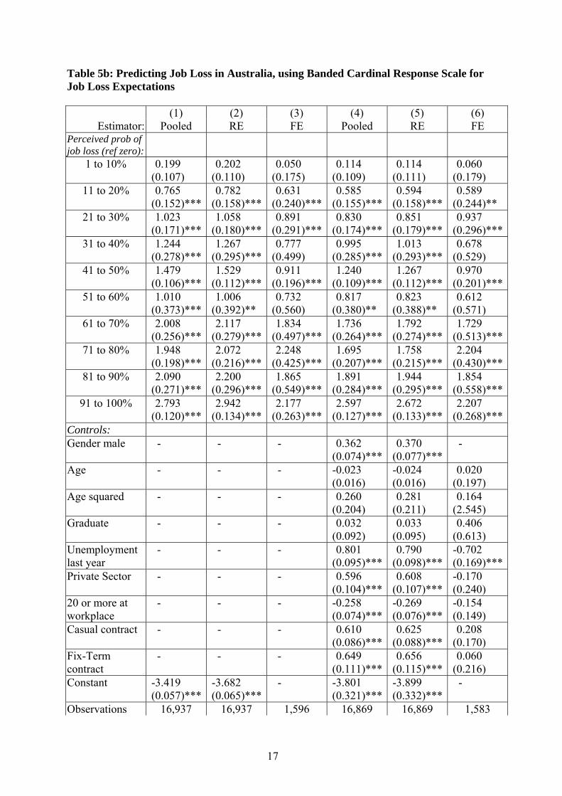
Table 5b: Predicting Job Loss in Australia, using Banded Cardinal Response Scale for Job Loss Expectations (1) (2) (3) (4) (5) (6)
Estimator: Pooled RE FE Pooled RE FE Perceived prob of job loss (ref zero):
1 to 10% 0.199 (0.107)
0.202 (0.110)
0.050 (0.175)
0.114 (0.109)
0.114 (0.111)
0.060 (0.179)
11 to 20% 0.765 (0.152)***
0.782 (0.158)***
0.631 (0.240)***
0.585 (0.155)***
0.594 (0.158)***
0.589 (0.244)**
21 to 30% 1.023 (0.171)***
1.058 (0.180)***
0.891 (0.291)***
0.830 (0.174)***
0.851 (0.179)***
0.937 (0.296)***
31 to 40% 1.244 (0.278)***
1.267 (0.295)***
0.777 (0.499)
0.995 (0.285)***
1.013 (0.293)***
0.678 (0.529)
41 to 50% 1.479 (0.106)***
1.529 (0.112)***
0.911 (0.196)***
1.240 (0.109)***
1.267 (0.112)***
0.970 (0.201)***
51 to 60% 1.010 (0.373)***
1.006 (0.392)**
0.732 (0.560)
0.817 (0.380)**
0.823 (0.388)**
0.612 (0.571)
61 to 70% 2.008 (0.256)***
2.117 (0.279)***
1.834 (0.497)***
1.736 (0.264)***
1.792 (0.274)***
1.729 (0.513)***
71 to 80% 1.948 (0.198)***
2.072 (0.216)***
2.248 (0.425)***
1.695 (0.207)***
1.758 (0.215)***
2.204 (0.430)***
81 to 90% 2.090 (0.271)***
2.200 (0.296)***
1.865 (0.549)***
1.891 (0.284)***
1.944 (0.295)***
1.854 (0.558)***
91 to 100% 2.793 (0.120)***
2.942 (0.134)***
2.177 (0.263)***
2.597 (0.127)***
2.672 (0.133)***
2.207 (0.268)***
Controls: Gender male - - - 0.362
(0.074)***0.370
(0.077)*** -
Age - - - -0.023 (0.016)
-0.024 (0.016)
0.020 (0.197)
Age squared - - - 0.260 (0.204)
0.281 (0.211)
0.164 (2.545)
Graduate - - - 0.032 (0.092)
0.033 (0.095)
0.406 (0.613)
Unemployment last year
- - - 0.801 (0.095)***
0.790 (0.098)***
-0.702 (0.169)***
Private Sector - - - 0.596 (0.104)***
0.608 (0.107)***
-0.170 (0.240)
20 or more at workplace
- - - -0.258 (0.074)***
-0.269 (0.076)***
-0.154 (0.149)
Casual contract - - - 0.610 (0.086)***
0.625 (0.088)***
0.208 (0.170)
Fix-Term contract
- - - 0.649 (0.111)***
0.656 (0.115)***
0.060 (0.216)
Constant -3.419 (0.057)***
-3.682 (0.065)***
- -3.801 (0.321)***
-3.899 (0.332)***
-
Observations 16,937 16,937 1,596 16,869 16,869 1,583
17

Individuals 7,546 608 7,529 605 Hausman test χ2(10)=24.7 χ2(18)=181.8Log likelihood -3257.6 -3241.8 -507.7 -3085.7 -3081.4 -493.2 Notes to Table 5: 1. These are logit estimates in each column. The Hausman test reported at the bottom of
column (3) and column (6) rejects RE over FE in both cases. 2. Coefficients estimated to be statistically significantly different from zero are denoted *, **
and *** for 10%, 5% and 1% respectively. d) Ordinal vs cardinal response scale? Finally in this section we examine the relative performance of the ordinal and cardinal response scales for the perceived risk of job loss in predicting actual job loss. In particular, we provide some measures of whether the use of the ordinal or the cardinal perception scale provides a ‘better’ predictive performance. Table 6 summarises our findings. Table 6a: Comparing the Ordinal and Cardinal Response scales No controls: With controls: Hosmer-Lemeshow Scale and year: Pseudo-R2 M&Z R2 Pseudo-R2 M&Z R2 χ2(8) p-value Nobs Ordinal scale:
1994 0.068 0.098 0.098 0.148 9.3 0.31 √ 7,3171996 0.091 0.122 0.120 0.177 16.9 0.03 × 7,4021998 0.099 0.128 0.158 0.224 14.6 0.07 √ 7,788
1994/1996/1998 0.085 0.115 0.121 0.177 31.3 0.00 × 22,507Cardinal scale: (continuous)
1999 0.091 0.132 0.137 0.202 2.6 0.95 √ 7,7792001 0.081 0.112 0.122 0.187 17.9 0.02 × 11,968
1999/2001 0.084 0.118 0.125 0.189 12.5 0.13 √ 19,747Cardinal scale: (discrete)
1999 0.097 0.119 0.142 0.193 13.2 0.10 √ 7,7792001 0.084 0.111 0.124 0.185 22.4 0.00 × 11,968
1999/2001 0.087 0.111 0.128 0.183 26.8 0.00 × 19,747 Notes: 1. The table reports the goodness-of-fit measures for the logit regressions of actual job loss
on perceived job loss for the GSOEP data for the years indicated in the first column. 2. Pseudo-R2 is the commonly reported McFadden (1973) measure based on the log
likelihoods; M&Z R2 is due to McKelvey and Zavoina (1975) (see text for details). 3. The control variables are identical to those in Table 3 and Table 4 above. 4. The Hosmer-Lemeshow test is a measure of goodness-of-fit similar to the conventional
Pearson χ2 test (see text for details). It has a χ2(8) distribution under the null hypothesis. At 5%, the critical value is χ2(8)=15.5.
There is a plethora of R2-type measures for limited dependent variable models such as the logit regressions presented here. Useful surveys are presented by Windmeijer (1995) and
18

Veall and Zimmermann (1996) amongst others. Table 6a reports two such R2 measures. The first is the most commonly employed Pseudo-R2 which is due to McFadden (1973), and is defined as the proportionate gain in the log-likelihood (relative to an intercept only model). The second measure is due to McKelvey and Zavoina (1975). This is of the ‘explained variation class’ of measures in that it mimics the standard R2 in OLS since it can be interpreted as the ratio of explained sum of squares to the total sum of squares (Veall and Zimmermann, 1996). Simulations suggest that this measure most closely approximates the OLS R2 for the underlying (unobserved) latent variable model (Hagel and Mitchell, 1992; Windmeijer, 1995) and hence it is an attractive choice.
The results for these two goodness-of-fit measures in Table 6a shows that, while year-by-year there is some variation, a comparison does not strongly suggest that the cardinal response scale is any better or worse, in general, than the ordinal response scale in predicting actual job loss. This conclusion holds whether or not the other control variables are also included in the logit regressions. Moreover, when the data are pooled for the ordinal and cardinal response scales (as in the regressions reported in Table 3, columns (1) and (4), and Tables 4a and 4b, columns (1) and (4)), once again there is no strong case for preferring either the ordinal or the cardinal response scale on the basis of their predictive performance, at least as measured by these two goodness-of-fit statistics.9
For the specifications with the control variables, we also report the Hosmer-Lemeshow goodness-of-fit test statistic. This is equivalent to the conventional Pearson chi-squared goodness-of-fit test10 for the case where the number of ‘cells’ (distinct covariate patterns) approaches N (the number of observations) as will be the case when we have many and/or continuous regressors. In such circumstances, the Pearson test is invalid since it relies on the expected number of observations per cell to be large. The Hosmer and Lemeshow (1980) test groups the observations into g = 10 deciles of risk based on their ordered estimated probabilities, and uses these 10 cells to compute a Pearson-like chi-squared test statistic comparing the observed and estimated number of cases per cell. Under the null – that the model is a good fit to the data – the resulting test statistic has a χ2(g-2) distribution.
The Hosmer-Lemeshow test statistics together with the p-values are reported for each of the years, and also for the data pooled for the ordinal and cardinal scales. The results again reveal some variation year-by-year, although with the cardinal scale treated as a continuous variable, the overall fit is acceptable while for the ordinal scale it is not. (However, perhaps somewhat surprisingly, when the cardinal scale is treated in a discrete fashion, the overall model fit is not acceptable, despite not having the constraint of linearity).
There is an important weakness in the above comparisons between the predictive performance of the ordinal and cardinal response scales. In estimating using separate cross-sections, or pooling the data, we are not comparing the same individuals using the different response scales. Thus, in Table 6b we restrict the analysis to individuals who appear both before and after the change in measurement scale from ordinal to cardinal. There are a number of ways of doing this. First, in Panel (A), we compare the predictive performance of all those who are in the sample of respondents in 1998 with their performance in 1999 if they are present. Second, in Panel (B), we compare the performance of the 1999 sample with that of those who had also been there in 1998. Finally, in Panel (C), we can compare the performance of only those who were present in both 1998 and 1999 by taking the relevant observations from Panel (A) and
9 We did examine alternative goodness-of-fit measures but these too did not provide conclusive evidence that the cardinal scale performs any better or worse than the ordinal scale. 10 That is, the test based on the sum of squared differences between the observed and expected number of cases per cell divided by its standard error.
19
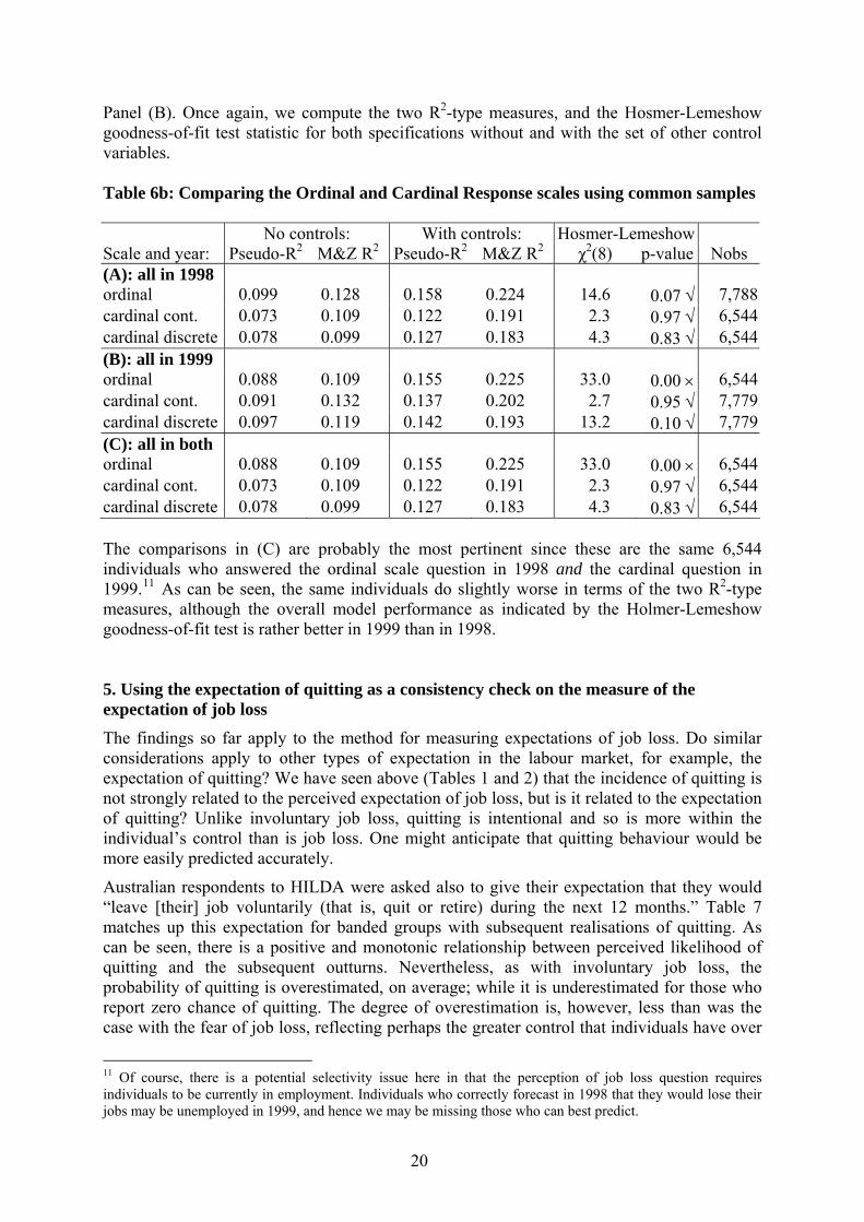
Panel (B). Once again, we compute the two R2-type measures, and the Hosmer-Lemeshow goodness-of-fit test statistic for both specifications without and with the set of other control variables. Table 6b: Comparing the Ordinal and Cardinal Response scales using common samples No controls: With controls: Hosmer-Lemeshow Scale and year: Pseudo-R2 M&Z R2 Pseudo-R2 M&Z R2 χ2(8) p-value Nobs (A): all in 1998 ordinal 0.099 0.128 0.158 0.224 14.6 0.07 √ 7,788cardinal cont. 0.073 0.109 0.122 0.191 2.3 0.97 √ 6,544cardinal discrete 0.078 0.099 0.127 0.183 4.3 0.83 √ 6,544(B): all in 1999 ordinal 0.088 0.109 0.155 0.225 33.0 0.00 × 6,544cardinal cont. 0.091 0.132 0.137 0.202 2.7 0.95 √ 7,779cardinal discrete 0.097 0.119 0.142 0.193 13.2 0.10 √ 7,779(C): all in both ordinal 0.088 0.109 0.155 0.225 33.0 0.00 × 6,544cardinal cont. 0.073 0.109 0.122 0.191 2.3 0.97 √ 6,544cardinal discrete 0.078 0.099 0.127 0.183 4.3 0.83 √ 6,544 The comparisons in (C) are probably the most pertinent since these are the same 6,544 individuals who answered the ordinal scale question in 1998 and the cardinal question in 1999.11 As can be seen, the same individuals do slightly worse in terms of the two R2-type measures, although the overall model performance as indicated by the Holmer-Lemeshow goodness-of-fit test is rather better in 1999 than in 1998. 5. Using the expectation of quitting as a consistency check on the measure of the expectation of job loss The findings so far apply to the method for measuring expectations of job loss. Do similar considerations apply to other types of expectation in the labour market, for example, the expectation of quitting? We have seen above (Tables 1 and 2) that the incidence of quitting is not strongly related to the perceived expectation of job loss, but is it related to the expectation of quitting? Unlike involuntary job loss, quitting is intentional and so is more within the individual’s control than is job loss. One might anticipate that quitting behaviour would be more easily predicted accurately.
Australian respondents to HILDA were asked also to give their expectation that they would “leave [their] job voluntarily (that is, quit or retire) during the next 12 months.” Table 7 matches up this expectation for banded groups with subsequent realisations of quitting. As can be seen, there is a positive and monotonic relationship between perceived likelihood of quitting and the subsequent outturns. Nevertheless, as with involuntary job loss, the probability of quitting is overestimated, on average; while it is underestimated for those who report zero chance of quitting. The degree of overestimation is, however, less than was the case with the fear of job loss, reflecting perhaps the greater control that individuals have over
11 Of course, there is a potential selectivity issue here in that the perception of job loss question requires individuals to be currently in employment. Individuals who correctly forecast in 1998 that they would lose their jobs may be unemployed in 1999, and hence we may be missing those who can best predict.
20

quitting. Table 7 also shows that there is a weak relationship between quit perception and subsequent job loss. Thus, only to a minor extent does job loss pre-empt an expected quit.
Table 7: Proportions of Employees Quitting and Losing Their Job, by Perceived Likelihood of Quitting in Australia, 2001-2003
Actual quits1 Job loss1 Perceived likelihood of quitting:1 (%) (s.e.) (%) (s.e.)
0% 8.7 (0.3) (4.7) (0.2) 1 to 10% 9.8 (0.7) (3.7) (0.4) 11 to 20% 14.2 (1.4) (5.2) (0.9) 21 to 30% 17.0 (1.7) (5.2) (1.0) 31 to 40% 21.9 (3.1) (7.9) (2.0) 41 to 50% 24.6 (1.0) (7.4) (0.6) 51 to 60% 29.9 (3.2) (4.9) (1.5) 61 to 70% 33.2 (2.8) (9.4) (1.7) 71 to 80% 33.8 (1.9) (7.4) (1.0) 81 to 90% 42.9 (2.6) (7.0) (1.3) 91 to 100% 50.3 (1.4) (12.3) (0.9)
Notes: 1. Time frame for perceived likelihood of quitting and actual quits and job loss is one year. 2. Standard errors (s.e.) are in parentheses. Mean (s.e.) perceived likelihood of quitting: 0.221 (0.003) Mean (s.e.) proportion quitting: 0.164 (0.003) Number of observations: 16,921 This finding is included here as additional evidence that respondents are able to make successful forecasts of future labour market states. We intend in future work to extend the analysis to other types of labour market expectation.
Of particular interest here, however, is the conjunction of job loss expectations with quit intentions, within the same questionnaire. There can be non-zero probabilities of both occurring for any individual. It would be illogical, however, for an individual to report perceived probabilities that sum to more than 100%, because the two outcomes are mutually exclusive. The questions on job loss and quitting expectations were asked one immediately after the other, but (as far as we can tell) no check is made during the interview to pre-empt any replies that are inconsistent in this way.
This fact allows a further check on the validity of the probability scale used in HILDA. It emerges that, in 5.5% of cases, the sum of the probabilities of job loss and quitting is greater than 100%. At the extreme, there were 203 cases (0.8%) over the four waves of people predicting that both events would happen with certainty, despite the fact that they are clearly mutually exclusive. This finding casts some doubt on how well even properly-formed questions are understood by a small minority of respondents. Note, however, that it is possible that similar inconsistencies might be revealed even when ordinal verbal scales are used; but in the ordinal scale period of GSOEP the various alternative expectations that are asked about are not mutually exclusive events.
21

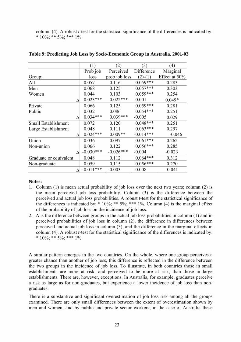
6. Extension: expectations and realisations of job loss among socio-economic groups In previous sections we have shown that individuals’ expectations of job loss provide information about their job loss chances over and above the conventional demographic and labour market information typically collected in survey work. In this final section we briefly extend the analysis by asking whether the expectations held by some groups of workers are more informative than those held by others. Following on from our brief review of the literature in Section 2, one might consider whether groups that are arguably more informed about the labour market are able to predict better. By a better prediction, in this case, we mean predictions that imply a lower degree of overestimation of actual job loss on average and at the margin.
Tables 8 and 9 show relevant descriptive statistics for Germany and Australia, using the cardinal scales. They give the mean perceived probability of job loss alongside the actual incidence of job loss, and the difference between these two, which is the extent of overestimation or pessimism on average. The final column gives the marginal effect, evaluated at the point where the perceived probability of job loss is 50%. If individuals in a group reported accurate information about their chances of job loss, this marginal effect would be 1.
Table 8: Predicting Job Loss by Socio-Economic Group in Germany, 1999 and 2001
(1) (2) (3) (4)
Group: Prob job
loss Perceived
prob job lossDifference
(2)-(1) Marginal
Effect at 50% All 0.0954 0.2049 0.1095*** 0.334 Men 0.0972 0.2009 0.1037*** 0.381 Women 0.0932 0.2098 0.1165*** 0.315
Δ 0.0040 -0.0089** -0.0129*** 0.0660*** Private 0.1069 0.2136 0.1067*** 0.316 Public 0.0571 0.1757 0.1187*** 0.339
Δ 0.0499*** 0.0378*** -0.0120*** -0.023 Small Establishment 0.1183 0.2175 0.0992*** 0.347 Large Establishment 0.0571 0.1838 0.1266*** 0.279
Δ 0.0612*** 0.0337*** -0.0274*** 0.068*** Graduate or equivalent 0.0720 0.1919 0.1199*** 0.326 Non-graduate 0.1048 0.2101 0.1052*** 0.333
Δ -0.0328*** -0.0181*** 0.0147*** 0.007 Notes: 1. Column (1) is mean actual probability of job loss over the next two years; column (2) is
the mean perceived job loss probability. Column (3) is the difference between the perceived and actual job loss probabilities. A robust t-test for the statistical significance of the differences is indicated by: * 10%; ** 5%; *** 1%. Column (4) is the marginal effect of the probability of job loss on the incidence of job loss.
2. Δ is the difference between groups in the actual job loss probabilities in column (1) and in perceived probabilities of job loss in column (2), the difference in differences between perceived and actual job loss in column (3), and the difference in the marginal effects in
22
column (4). A robust t-test for the statistical significance of the differences is indicated by: * 10%; ** 5%; *** 1%.
Table 9: Predicting Job Loss by Socio-Economic Group in Australia, 2001-03
(1) (2) (3) (4)
Group: Prob job
loss Perceived
prob job lossDifference
(2)-(1) Marginal
Effect at 50% All 0.057 0.116 0.059*** 0.283 Men 0.068 0.125 0.057*** 0.303 Women 0.044 0.103 0.059*** 0.254
Δ 0.023*** 0.022*** 0.001 0.049* Private 0.066 0.125 0.059*** 0.281 Public 0.032 0.086 0.054*** 0.251
Δ 0.034*** 0.039*** -0.005 0.029 Small Establishment 0.072 0.120 0.048*** 0.251 Large Establishment 0.048 0.111 0.063*** 0.297
Δ 0.024*** 0.009** -0.014*** -0.046 Union 0.036 0.097 0.061*** 0.262 Non-union 0.066 0.122 0.056*** 0.285
Δ -0.030*** -0.026*** -0.004 -0.023 Graduate or equivalent 0.048 0.112 0.064*** 0.312 Non-graduate 0.059 0.115 0.056*** 0.270
Δ -0.011*** -0.003 -0.008 0.041 Notes: 1. Column (1) is mean actual probability of job loss over the next two years; column (2) is
the mean perceived job loss probability. Column (3) is the difference between the perceived and actual job loss probabilities. A robust t-test for the statistical significance of the differences is indicated by: * 10%; ** 5%; *** 1%. Column (4) is the marginal effect of the probability of job loss on the incidence of job loss.
2. Δ is the difference between groups in the actual job loss probabilities in column (1) and in perceived probabilities of job loss in column (2), the difference in differences between perceived and actual job loss in column (3), and the difference in the marginal effects in column (4). A robust t-test for the statistical significance of the differences is indicated by: * 10%; ** 5%; *** 1%.
A similar pattern emerges in the two countries. On the whole, where one group perceives a greater chance than another of job loss, this difference is reflected in the difference between the two groups in the incidence of job loss. To illustrate, in both countries those in small establishments are more at risk, and perceived to be more at risk, than those in large establishments. There are, however, exceptions. In Australia, for example, graduates perceive a risk as large as for non-graduates, but experience a lower incidence of job loss than non-graduates.
There is a substantive and significant overestimation of job loss risk among all the groups examined. There are only small differences between the extent of overestimation shown by men and women, and by public and private sector workers; in the case of Australia these
23
differences are statistically insignificant. In contrast, those working in small establishments are significantly closer to reality in their expectations of job loss than those in large establishments. In addition, in Germany the marginal expectation (at 50%) is somewhat greater for small than for large establishments. One might interpret these findings about both the average and the marginal expectation as possibly attributable to those in smaller establishments being better informed, perhaps through informal channels, of labour market developments. However, there are no differences in the marginal expectation in Australia.
Taking these results together, they provide only very weak support for the proposition that some groups of workers may be better informed than others and hence able to form more accurate expectations of their future job security.
7. Conclusions The measurement of expectations of labour market agents is potentially valuable as a tool for analysing a wide range of labour market behaviour. We have focussed on the expectation of job loss, since this is an important ingredient of the wider concept of job insecurity. There is a good case for using questions that unambiguously capture this risk, without conflating it with subsequent possibilities (for example, the uncertain cost of job loss). Conflation with other related risks reduces the validity of the instrument, because it induces ambiguity. In addition it is known that if some respondents, asked to report the joint likelihood of two risks, are liable to commit the conjunction fallacy.
When measuring workers’ expectations of job loss one might opt to defend any format that successfully elicits expectations, whether or not the expressed expectations are realised. If workers say they have a high fear of job loss this might affect their behaviour even if that fear is not warranted. However, if the intention of a survey design is to obtain measures of anxiety or worry it is probably best to turn to already-tested instruments in the field of psychology. Normally, economists will find expressions about labour market expectations of interest if they convey private information – that is, information about the respondents’ particular circumstances or personal intentions that would not typically be collected in other ways by researchers external to the subject’s workplace.
In this light, the finding reported here that the expectations of job loss questions in GSOEP and HILDA are additionally informative about the probability of subsequent job loss provides solid support for the value of such questions in labour market analysis. By extending this insight, previously found in Canada and Britain, to two further substantial labour forces, there can be some considerable confidence in the use of such expectations questions. Moreover, by showing for the first time that the predictive power of the expectations data holds using a fixed-effects panel estimator, this paper makes the insight that much stronger.
Despite the predictive power of the expectations questions, we have also found a pattern of pessimism (over-estimation of the chance of job loss) for all workers who have any fear of job loss, while those who think that they have no chance at all of job loss underestimate the small risk they face. Again, German and Australian workers appear to be similar in this respect to British and Canadian workers. Those working in large establishments are more pessimistic than those in small workplaces. The pessimism in all cases is genuine in the sense that it is not a statistical artefact arising from strategic quitting; nor is it merely a consequence of a mistiming of the period over which job loss is expected. We have not investigated the origins of this pessimism, preferring to leave this field of enquiry to psychologists better qualified to frame the right questions and experiments. One predicted effect of pessimism would be to
24

generate an excess demand for unemployment insurance, though the extent of this effect will depend on the potential costs of job loss.
We have also addressed whether cardinal scales, expressing the perceived probability of job loss, are methodologically superior to ordinal scales with verbal descriptors. Cardinal scales are in principle preferable, because the meaning of numerical scale points is unambiguous while that of verbal descriptors might differ among respondents if their understanding of language is heterogeneous, or if the words are vague. Moreover, cardinal scales offer analytical advantages, in that marginal changes in probability are commensurate along the scale, which is not true of ordinal verbal descriptors. Nevertheless, it was an open question as to whether the responses on cardinal scales are reliable.
The analysis of realisations is not wholly favourable to the use of cardinal scales. We have compared goodness-of-fit measures in GSOEP from before and after the switch from ordinal to cardinal scales, and found no strong case to choose between them on these grounds. We have also found no evidence that, where a comparison is possible, a cardinal scale elicits a substantively lower level of pessimism than an ordinal scale. If these were the only findings we would nevertheless recommend cardinal scales on the grounds that they have greater face validity, and that their predictive power is no worse than that of ordinal scales. However, further analysis of the cardinal scale results showed that the relationship to job loss incidence was non-linear. This finding implies that it would not be reliable to treat a marginal change in job loss expectations as proportional to a marginal change in the objective incidence of job loss. Moreover, there is reason to doubt the reliability of the perceptions of those who place themselves just away from the focal point of 50%, and even more so of those few who report off-decile-point perceptions.
In light of this finding, we recommend the use of discrete scale points for questions on job loss expectations. These scale points should be taken as ordinally ranked descriptors of job loss probabilities in analyses, rather than cardinal probability measures. Given the lumpiness of responses to the HILDA and GSOEP scales, and the unreliability of some of the ‘off-spike’ points, it also seems advisable to utilise rather less than ten scale points. Whether the descriptors of the scale points should be verbal or numerical, however, is not prescribed by the evidence here. There may therefore be merit in utilising numerical banded scales, which will have better face validity than the less precise verbal descriptors commonly used. Alternatively, there is an argument for combining the verbal and numerical approach, by attaching probability bands to verbal descriptors.
There remains scope for expanding the analysis of expectations in the labour market to further domains. Closely related to the present paper is another major component of job insecurity, the probability of succeeding or failing to regain employment of similar quality. While several surveys elicit expectations in this domain, the reliability of the responses has yet to be confirmed. HILDA also collects data on the job-gaining expectations of unemployed people – the reverse of the transition examined in this paper. GSOEP collects information on other possibilities for employees such as the chances of promotion or demotion. As part of an investigation of the uncertainty associated with job insecurity, we are analysing the reliability of this expectations data in ongoing work.
25
References Benito, A. (2004). Does job insecurity affect household consumption?, Working Paper No.
220, Structural Economic Analysis Division, Bank of England.
Bryson, A., L. Cappellari and C. Lucifora (2004). Do Job Security Guarantees Work?, London School of Economics, Centre for Economic Performance, Discussion Paper 661.
Campbell, D., A. Carruth, A. Dickerson and F. Green (forthcoming 2007). “Job Insecurity and Wages.” Economic Journal.
Carroll, C D, Dynan, K E and Krane, S D (2003), ‘Unemployment risk and precautionary wealth: evidence from households’ balance sheets’, Review of Economics and Statistics, Vol. 85, pages 586-604.
Clarke, A. E. and F. Postel-Vinay (2004). Job Security and Job Protection, DELTA, Working Paper No. 2004-16, Paris.
Constans, J. I. (2001). “Worry propensity and the perception of risk.” Behaviour Research and Therapy 39: 721-729.
Erev, I. and B. Cohen (1990) “Verbal versus numerical probabilities: efficiency, Biases and the preference paradox”, Organizational Behavior and Human Decision Processes, 45, 1-18.
Green, F. (2006). Demanding Work. The Paradox of Job Quality in the Affluent Economy. Woodstock, Princeton University Press.
Green, F., B. Burchell and A. Felstead (2000). “Job insecurity and the difficulty of regaining employment: an empirical study of unemployment expectations.” Oxford Bulletin of Economics and Statistics 62 (December): 855-884.
Hagle T. M. and G. E. Mitchell (1992), “Good-of-fit measures for Probit and Logit”, American Journal of Political Science, 36, pp.762-784
Hosmer D. W. and S. Lemeshow (1980), “Goodness-of-fit test for the multiple logistic regression model”, Communications in Statistics: Theory and Methods Part A, 9, pp.1043-1069.
Hurd, M.D. and McGarry, K. (2002). “The Predictive Validity of Subjective Probabilities of Survival”, Economic Journal, 112, No. 482, October, 966-987.
Long, J. S. (1997). Regression Models for Categorical and Limited Dependent Variables. Thousand Oaks, CA: Sage Publications.
Lukasiewicz E, Fischler C, Setbon M, Flahault A (2001) Comparison of three scales to assess health risk perception, Revue D’Epidemiologie Et De Sante Publique 49 (4): 377-385 September.
Lusardi, A (1998), ‘On the importance of the precautionary saving motive’, American Economic Review, Papers and Proceedings, Vol. 88, pages 449-53.
Manski, C. F. (2004). “Measuring Expectations.” Econometrica 72(5): 1329-1376.
Manski, C.F. and Straub, J. D. (2000) “Worker Perceptions of Job Insecurity in the Mid-1990s”, Journal of Human Resources, 35 (3), 447-479.
McFadden D. (1973), “Conditional Logit Analysis of Qualitative Choice Behavior", in Zarembka P. (ed.), Frontiers in Econometrics, pp.105-142, Academic Press, New York.
26
McKelvey, R., and Zavoina, W. (1975) “A Statistical Model for the Analysis of Ordinal Level Dependent Variables”, Journal of Mathematical Sociology 4, pp. 103-120.
Rutter, D. R., Quine, L. and I.P. Albery (1998) “Perceptions of risk in motorcyclists: Unrealistic optimism, relative realism and predictions of behaviour”, British Journal of Psychology, 89, 681-696.
Schmidt, S. R. (1999) “Long-Run Trends in Workers’ Beliefs about Their Own Job Security: Evidence from the General Social Survey”, Journal of Labour Economics, 17 (4), Part 2, S127-S141.
Stephens, M. Jr. (2004), “Job loss expectations,. realizations and household consumption behaviour”, Review of Economics and Statistics, 86(1): 253-269.
Veall, M.R. and K.F. Zimmermann (1996), “Pseudo-R2 Measures for Some Common Limited Dependent Variable Models”, Journal of Economic Surveys, Vol. 10, No. 3, 241-259.
Weinstein N. D., S. E. Marcus and R. P. Moser (2005) “Smokers' unrealistic optimism about their risk”, Tobacco Control 14 (1): 55-59.
Windmeijer F. A. G. (1995), “Goodness-of-fit measures in Binary Choice Models” Econometric Reviews, 14, pp.101-116.
Wichert, I. (2002) Job insecurity and work intensification : the effects on health and well-being. Job Insecurity And Work Intensification. Burchell, B., Ladipo, D, and Wilkinson, F. London and New York, Routledge: 92-111.
Winship, C. and R. D. Mare.(1984) “Regression Models with Ordinal Variables.” American Sociological Review 49(August): 512–525.
27