How multiple supernovae overlap to form superbubbles … · How multiple supernovae overlap to form superbubbles ... injection of mechanical energy by massive stars in the form of

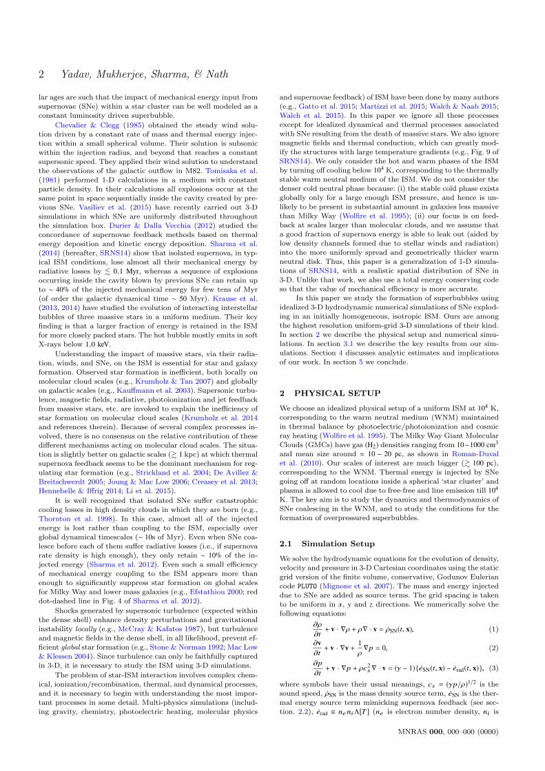
MNRAS 000, 000–000 (0000) Preprint 21 June 2017 Compiled using MNRAS LATEX style file v3.0

How multiple supernovae overlap to form superbubbles

Naveen Yadav1?, Dipanjan Mukherjee2†, Prateek Sharma1‡ and Biman B. Nath31Department of Physics & Joint Astronomy Programme, Indian Institute of Science, Bangalore, India -560012.2Research School of Astronomy & Astrophysics, Mount Stromlo Observatory, ACT 2611, Australia.3Raman Research Institute, Sadashiva Nagar, Bangalore, India -560080.

21 June 2017

ABSTRACTWe explore the formation of superbubbles through energy deposition by multiple su-pernovae (SNe) in a uniform medium. We use total energy conserving, 3-D hydrody-namic simulations to study how SNe correlated in space and time create superbubbles.While isolated SNe fizzle out completely by ∼ 1 Myr due to radiative losses, for a re-alistic cluster size it is likely that subsequent SNe go off within the hot/dilute bubbleand sustain the shock till the cluster lifetime. For realistic cluster sizes, we find thatthe bubble remains overpressured only if, for a given ng0, NOB is sufficiently large.While most of the input energy is still lost radiatively, superbubbles can retain upto ∼ 5 − 10% of the input energy in form of kinetic+thermal energy till 10 Myr forISM density ng0 ≈ 1 cm−3. We find that the mechanical efficiency decreases for higher

densities (ηmech ∝ n−2/3g0 ). We compare the radii and velocities of simulated supershells

with observations and the classical adiabatic model. Our simulations show that the su-perbubbles retain only . 10% of the injected energy, thereby explaining the observedsmaller size and slower expansion of supershells. We also confirm that a sufficientlylarge (& 104) number of SNe is required to go off in order to create a steady windwith a stable termination shock within the superbubble. We show that the mechanicalefficiency increases with increasing resolution, and that explicit diffusion is requiredto obtain converged results.

Key words: Hydrodynamics – Methods: numerical – ISM: bubbles.

1 INTRODUCTION

HI holes, shells, rings, expanding cavities, galactic chimneys, and

filaments are ubiquitous structures which are embedded in the

large scale gas distribution of a galaxy. Heiles (1979) identifiedlarge cavities in the local interstellar medium (ISM) with energy

requirement of & 3 × 1052 erg as supershells. Our solar system isitself embedded in such a cavity (radius ∼ 100 pc) filled with hot(∼ 106 K) and tenuous (n ∼ 5 × 10−3 cm−3) plasma (Sanders et al.

1977; McCammon et al. 1983) known as the local hot bubble(LHB).

When the size of a superbubble becomes comparable to the

galactic HI scale height, it may break out of the galactic disk ifthe shell is sufficiently fast (e.g., Mac Low & McCray 1988; Roy

et al. 2013) and inject energy and metals into the galactic halo.The widely accepted model of galaxy-scale superwinds involvesinjection of mechanical energy by massive stars in the form of

radiation (L?), stellar winds (Lw) and supernova (SN) explosions

(ESN ∼ 1051 erg). Clearly, such large cavities cannot be created byeither the wind from a single massive star or by the supernovaexplosion of a single star. Further it is known from observations

? [email protected]† [email protected]‡ [email protected]

of O-type stars in the Galaxy that ∼ 70% of them are associated

with clusters and OB associations and a very small fraction ofthe known O-stars are isolated (Chu & Gruendl 2008). Out of

the remaining 30%, more than one-third are runaway stars which

have been ejected in close gravitational encounters (Gies 1987).Hence the most plausible mechanism for the formation of largesuperbubbles is quasi-continuous energy injection from multiple

stars. The expanding shells of each individual star/SN merge toform a large scale bubble known as a superbubble.

Pikel’Ner (1968); Avedisova (1972) studied the interaction

of a strong stellar wind with the interstellar medium (ISM). Thecircumstellar shell enters the snowplow phase when the radiativecooling timescale for the swept gas becomes equal to the dynam-

ical age of the shell. Weaver et al. (1977) calculated the detailed

structure for interaction of a strong stellar wind with the inter-stellar medium. Castor et al. (1975) obtained a solution for the

case of continuous energy injection (at a point) inside a homo-geneous medium by a stellar wind (Lw = ÛMv2

w/2) in the absenceof radiative energy losses and found the presence of a transition

region dominated by thermal conduction between the cold outerlayer of the shell (shocked ISM) and the hot inner layer of the

shell (shocked stellar wind). Weaver et al. (1977) analytically cal-culated detailed structure of the bubble in various phases of evolu-tion, including the effects of radiative cooling. McCray & Kafatos

(1987) highlighted that the stellar initial mass function and stel-

© 0000 The Authors

arX

iv:1

603.

0081

5v3

[as

tro-

ph.H

E]

20

Jun

2017

2 Yadav, Mukherjee, Sharma, & Nath

lar ages are such that the impact of mechanical energy input from

supernovae (SNe) within a star cluster can be well modeled as a

constant luminosity driven superbubble.

Chevalier & Clegg (1985) obtained the steady wind solu-

tion driven by a constant rate of mass and thermal energy injec-tion within a small spherical volume. Their solution is subsonic

within the injection radius, and beyond that reaches a constant

supersonic speed. They applied their wind solution to understandthe observations of the galactic outflow in M82. Tomisaka et al.

(1981) performed 1-D calculations in a medium with constant

particle density. In their calculations all explosions occur at thesame point in space sequentially inside the cavity created by pre-

vious SNe. Vasiliev et al. (2015) have recently carried out 3-Dsimulations in which SNe are uniformly distributed throughout

the simulation box. Durier & Dalla Vecchia (2012) studied the

concordance of supernovae feedback methods based on thermalenergy deposition and kinetic energy deposition. Sharma et al.

(2014) (hereafter, SRNS14) show that isolated supernova, in typ-

ical ISM conditions, lose almost all their mechanical energy byradiative losses by . 0.1 Myr, whereas a sequence of explosions

occurring inside the cavity blown by previous SNe can retain up

to ∼ 40% of the injected mechanical energy for few tens of Myr(of order the galactic dynamical time ∼ 50 Myr). Krause et al.

(2013, 2014) have studied the evolution of interacting interstellar

bubbles of three massive stars in a uniform medium. Their keyfinding is that a larger fraction of energy is retained in the ISM

for more closely packed stars. The hot bubble mostly emits in softX-rays below 1.0 keV.

Understanding the impact of massive stars, via their radia-tion, winds, and SNe, on the ISM is essential for star and galaxy

formation. Observed star formation is inefficient, both locally on

molecular cloud scales (e.g., Krumholz & Tan 2007) and globallyon galactic scales (e.g., Kauffmann et al. 2003). Supersonic turbu-

lence, magnetic fields, radiative, photoionization and jet feedback

from massive stars, etc. are invoked to explain the inefficiency ofstar formation on molecular cloud scales (Krumholz et al. 2014

and references therein). Because of several complex processes in-

volved, there is no consensus on the relative contribution of thesedifferent mechanisms acting on molecular cloud scales. The situa-

tion is slightly better on galactic scales (& 1 kpc) at which thermal

supernova feedback seems to be the dominant mechanism for reg-ulating star formation (e.g., Strickland et al. 2004; De Avillez &

Breitschwerdt 2005; Joung & Mac Low 2006; Creasey et al. 2013;

Hennebelle & Iffrig 2014; Li et al. 2015).

It is well recognized that isolated SNe suffer catastrophic

cooling losses in high density clouds in which they are born (e.g.,Thornton et al. 1998). In this case, almost all of the injected

energy is lost rather than coupling to the ISM, especially overglobal dynamical timescales (∼ 10s of Myr). Even when SNe coa-lesce before each of them suffer radiative losses (i.e., if supernovarate density is high enough), they only retain ∼ 10% of the in-jected energy (Sharma et al. 2012). Even such a small efficiency

of mechanical energy coupling to the ISM appears more than

enough to significantly suppress star formation on global scalesfor Milky Way and lower mass galaxies (e.g., Efstathiou 2000; red

dot-dashed line in Fig. 4 of Sharma et al. 2012).

Shocks generated by supersonic turbulence (expected within

the dense shell) enhance density perturbations and gravitationalinstability locally (e.g., McCray & Kafatos 1987), but turbulenceand magnetic fields in the dense shell, in all likelihood, prevent ef-ficient global star formation (e.g., Stone & Norman 1992; Mac Low

& Klessen 2004). Since turbulence can only be faithfully capturedin 3-D, it is necessary to study the ISM using 3-D simulations.

The problem of star-ISM interaction involves complex chem-ical, ionization/recombination, thermal, and dynamical processes,

and it is necessary to begin with understanding the most impor-

tant processes in some detail. Multi-physics simulations (includ-ing gravity, chemistry, photoelectric heating, molecular physics

and supernovae feedback) of ISM have been done by many authors(e.g., Gatto et al. 2015; Martizzi et al. 2015; Walch & Naab 2015;

Walch et al. 2015). In this paper we ignore all these processesexcept for idealized dynamical and thermal processes associated

with SNe resulting from the death of massive stars. We also ignore

magnetic fields and thermal conduction, which can greatly mod-ify the structures with large temperature gradients (e.g., Fig. 9 of

SRNS14). We only consider the hot and warm phases of the ISM

by turning off cooling below 104 K, corresponding to the thermallystable warm neutral medium of the ISM. We do not consider the

denser cold neutral phase because: (i) the stable cold phase exists

globally only for a large enough ISM pressure, and hence is un-likely to be present in substantial amount in galaxies less massive

than Milky Way (Wolfire et al. 1995); (ii) our focus is on feed-

back at scales larger than molecular clouds, and we assume thata good fraction of supernova energy is able to leak out (aided by

low density channels formed due to stellar winds and radiation)

into the more uniformly spread and geometrically thicker warmneutral disk. Thus, this paper is a generalization of 1-D simula-

tions of SRNS14, with a realistic spatial distribution of SNe in3-D. Unlike that work, we also use a total energy conserving code

so that the value of mechanical efficiency is more accurate.

In this paper we study the formation of superbubbles usingidealized 3-D hydrodynamic numerical simulations of SNe explod-

ing in an initially homogeneous, isotropic ISM. Ours are among

the highest resolution uniform-grid 3-D simulations of their kind.In section 2 we describe the physical setup and numerical simu-

lations. In section 3.1 we describe the key results from our sim-

ulations. Section 4 discusses analytic estimates and implicationsof our work. In section 5 we conclude.

2 PHYSICAL SETUP

We choose an idealized physical setup of a uniform ISM at 104 K,

corresponding to the warm neutral medium (WNM) maintainedin thermal balance by photoelectric/photoionization and cosmic

ray heating (Wolfire et al. 1995). The Milky Way Giant Molecular

Clouds (GMCs) have gas (H2) densities ranging from 10−1000 cm3

and mean size around ≈ 10 − 20 pc, as shown in Roman-Duval

et al. (2010). Our scales of interest are much bigger (& 100 pc),

corresponding to the WNM. Thermal energy is injected by SNegoing off at random locations inside a spherical ‘star cluster’ and

plasma is allowed to cool due to free-free and line emission till 104

K. The key aim is to study the dynamics and thermodynamics ofSNe coalescing in the WNM, and to study the conditions for the

formation of overpressured superbubbles.

2.1 Simulation Setup

We solve the hydrodynamic equations for the evolution of density,

velocity and pressure in 3-D Cartesian coordinates using the static

grid version of the finite volume, conservative, Godunov Euleriancode PLUTO (Mignone et al. 2007). The mass and energy injecteddue to SNe are added as source terms. The grid spacing is taken

to be uniform in x, y and z directions. We numerically solve thefollowing equations:

∂ρ

∂t+ v · ∇ρ + ρ∇ · v = ÛρSN(t, x), (1)

∂v∂t+ v · ∇v +

1ρ∇p = 0, (2)

∂p

∂t+ v · ∇p + ρc2

s∇ · v = (γ − 1){ ÛeSN(t, x) − Ûerad(t, x)}, (3)

where symbols have their usual meanings, cs = (γp/ρ)1/2 is the

sound speed, ÛρSN is the mass density source term, ÛeSN is the ther-mal energy source term mimicking supernova feedback (see sec-

tion. 2.2), Ûerad ≡ neniΛ[T ] (ne is electron number density, ni is

MNRAS 000, 000–000 (0000)

Supernovae to Superbubbles 3

ion number density and Λ[T ] is the temperature-dependent cool-

ing function) is the rate of energy loss per unit volume due to

radiative cooling. We use the ideal gas equation

ρε =p

(γ − 1) (4)

with γ = 5/3 (ε is internal energy per unit mass).

PLUTO solves the system of conservation laws which can be

written as

∂u∂t= −∇ ·Π + S, (5)

where u is a vector of conserved quantities, Π is the flux tensorand S is the source term. The system of equations is integrated

using finite volume methods. The temporal evolution of Eq. 5 iscarried by explicit methods and the time step is limited by the

Courant-Friedrichs-Lewy (CFL; Courant et al. 1928) condition.

The code implements time-dependent optically thin cooling ( Ûeradin Eq. 3) and the source terms ( ÛρSN in Eq. 1 and ÛeSN in Eq. 3)

via operator splitting. Our results are unaffected by boundary

conditions because we ensure that our box-size is large enoughsuch that the outer shock is sufficiently inside the computational

domain. We use the HLLC Riemann solver (Toro et al. 1994).

The solution is advanced in time using a second order Runge-Kutta (RK2) scheme and a total variation diminishing (TVD)

linear interpolation is used. The CFL number is set to 0.3 for nu-

merical stability. The computational domain is initialized with aninterstellar medium (ISM) of uniform density (ng0), with a mean

molecular weight per particle µ = 0.603 (mean molecular weightper electron µe = 1.156) and solar metallicity at a temperature of

104 K.

We have used the cooling module of PLUTO with the solarmetallicity cooling table of Sutherland & Dopita 1993).The cool-

ing function is set to zero below 104 K. We do not include self-

gravity, disk stratification, magnetic fields, and any form of gasheating (except by thermal energy injection due to SNe) in our

simulations.

We have two types of simulation setups:

• Full box: The full box simulations have a computational

domain extending from −L to +L in all three directions. Out-flow boundary conditions are used at the boundary of the com-

putational box (i.e., the planes x = −L, +L, y = −L, +L and

z = −L, +L).

• Octant: In octant simulations the simulation box extends

from 0 to +L along the three directions. We inject SNe in aspherical ‘star cluster’ centred at the origin, and the outcomes

are spherically symmetric in a statistical sense. Therefore, thesesimulations are statistically equivalent to the full box simulations,

but are computationally less expensive by roughly a factor of 8.These simulations are only carried out for a large number of SNe(NOB ≥ 103) because of a larger spatial stochasticity for smallnumber of SNe; for small NOB, an octant may have an effective

number of SNe which is substantially different from NOB/8. Forprecise mass and energy budgeting, we account for the actual

mass and energy dumped in by SNe in all cases. Reflective bound-ary conditions are used at the faces intersecting within the ‘starcluster’ (i.e., the planes x = 0, y = 0 and z = 0).

2.2 Supernova Energy Injection

In our setup, supernovae explode within a ‘star cluster’, a spher-ical region of radius rcl centred at the origin of the simulation

box. Most young star clusters are . 10 pc in size (e.g., see Larsen

1999) but we allow rcl to be larger. A larger rcl crudely mimicsa collection of star clusters that powers global galactic outflows

such as in M82 (O’Connell et al. 1995). The locations of SNe arechosen randomly, distributed uniformly within a sphere of radius

rcl, using the uniform random number generator ran2 (Press et al.

1986). Supernovae are injected uniformly in time, with the time

separation between successive SNe given by

δtSN =τOBNOB

, (6)

where τOB (chosen to be 30 Myr) is the life time of the OB as-sociation and NOB is the total number of SNe (which equals the

total number of O and B stars). Ferrand & Marcowith 2010 haveshown that statistically the supernova rate is uniform. McCray

& Kafatos 1987 also show that a constant mechanical luminosity

is a good approximation to supernova energy injection. Also, ithelps to understand the numerical results with simple analytic

calculations.

Each SN deposits a mass of MSN = 5 M� and internal energy

of ESN = 1051 erg over a sphere of size rSN = 5 pc; the SN en-

ergy injection radius is chosen to prevent artificial cooling losses(see Eq. 7 in SRNS14, corresponding to their thermal explosion

model). SRNS14 found that the late time (after a SN enters the

Sedov-Taylor stage) results are independent of whether SN en-ergy is deposited as kinetic or thermal energy (see their Figs. 2

& 3), so we simply deposit thermal energy.

Mass and energy injection from each SN is spread in space

and time using a Gaussian kernel, such that the mass and internal

energy source terms ( ÛρSN in Eq. 1 and ÛeSN in Eq. 3) are propor-tional to exp(−[t − ti]2/δt2

inj) × exp(−[x − xi]2/r2SN), where ith SN is

centred at ti in time and at xi in space. The injection timescale ischosen to be δtinj = δtSN/10. SN injection with smoothing is found

to be numerically more robust and the results are insensitive to

the details of smoothing. In addition to thermal energy, we de-posit a subdominant amount of kinetic energy because the mass

that we add in each grid cell (Eq. 1) is added at the local velocity.

We account for this additional energy in our energy budget.

We have carried out simulations with different values of ini-

tial ambient density (ng0), cluster size (rcl) and number of super-novae (NOB). The physical size of the simulation box is chosen

according to the number of SNe and the ambient density (based

on the adiabatic bubble formula of McCray & Kafatos 1987, theouter shock radius rsb ∝ [NOBt

3/ng0]1/5). All our 3-D simulations

are listed in Table B1 (convergence runs for the fiducial parame-ters, NOB = 100, ng0 = 1 cm−3, rcl = 100 pc) and Table 1 (all other

runs).

3 RESULTS

3.1 The fiducial Run

In this section we describe in detail the morphology and evolu-tion of a superbubble for number of SNe NOB = 100, initial gas

density ng0 = 1 cm−3, and cluster radius rcl = 100 pc, which we

choose as our fiducial run. The assumed parameters are typical ofsupershells (e.g., Heiles 1979; Suad et al. 2014; Bagetakos et al.

2011), but as mentioned earlier, rcl is larger than typical clus-ter sizes. Our spatial resolution is δL = 2.54 pc (run R2.5 in

Table B1). Simulations with different NOB and ng0 evolve in a

qualitatively similar fashion, the differences being highlighted insection 3.4. Numerical resolution quantitively affects our results,

although the qualitative trends remain similar. Strict convergence

is not expected because thermal and viscous diffusion are requiredto resolve the turbulent boundary layers connecting hot and warm

phases (e.g., Koyama & Inutsuka 2004). A detailed convergence

study is presented in Appendix B. Fig. 1 shows the gas densityand pressure slices in the midplane of the simulation domain at

times when SNe are effectively isolated (1.27 Myr) and when they

have coalesced (9.55 Myr) to form an overpressured superbubble.Since the evolution of a single SN is well known (see, e.g., Figs.

1 & 2 in Kim & Ostriker 2015), in order to compare with super-bubble evolution we just briefly review the different phases of SN

evolution. A SN shock starts in the free-expansion phase, moving

MNRAS 000, 000–000 (0000)


−300

−200

−100

0

100

200

300

y[p

c]

t = 1. 27 Myr t = 1. 27 Myr

−300 −200 −100 0 100 200 300

x [pc]

−300

−200

−100

0

100

200

300

y[p

c]

t = 9. 55 Myr

-5.3 -4.5 -3.8 -3.0 -2.2 -1.5 -0.8 0.0

log10ng (cm-3)

−300 −200 −100 0 100 200 300

x [pc]

t = 9. 55 Myr

0.0 1.0 2.0 3.0 4.0 5.0 6.0 7.0 8.0

pressure (10-12

dyne cm-2)

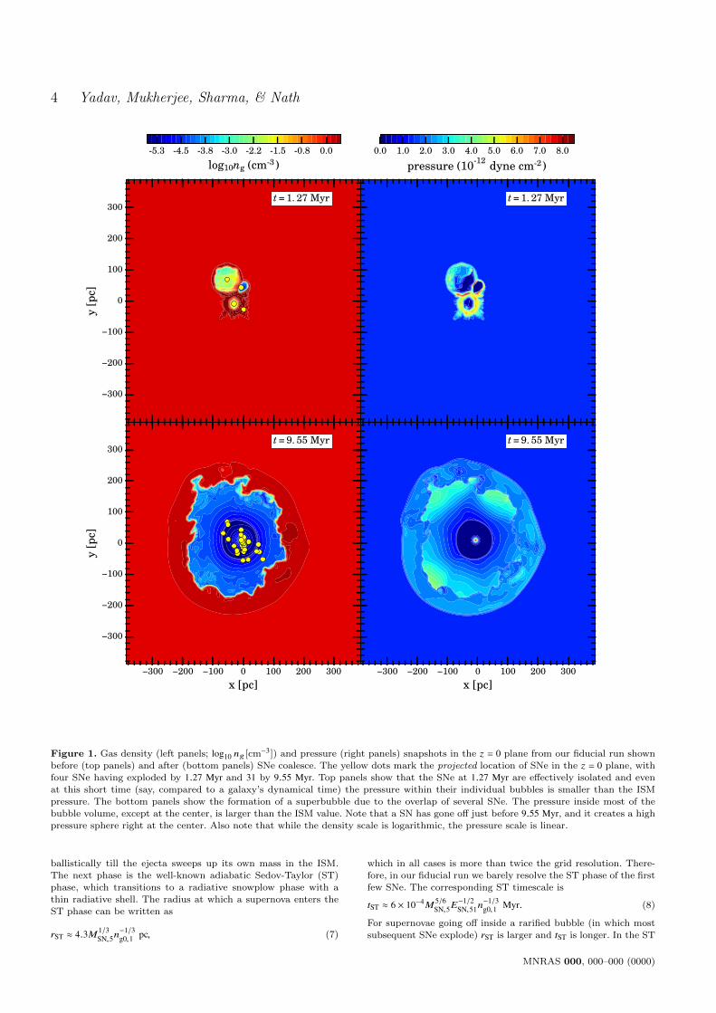
Figure 1. Gas density (left panels; log10 ng [cm−3]) and pressure (right panels) snapshots in the z = 0 plane from our fiducial run shown

before (top panels) and after (bottom panels) SNe coalesce. The yellow dots mark the projected location of SNe in the z = 0 plane, withfour SNe having exploded by 1.27 Myr and 31 by 9.55 Myr. Top panels show that the SNe at 1.27 Myr are effectively isolated and even

at this short time (say, compared to a galaxy’s dynamical time) the pressure within their individual bubbles is smaller than the ISMpressure. The bottom panels show the formation of a superbubble due to the overlap of several SNe. The pressure inside most of thebubble volume, except at the center, is larger than the ISM value. Note that a SN has gone off just before 9.55 Myr, and it creates a highpressure sphere right at the center. Also note that while the density scale is logarithmic, the pressure scale is linear.

ballistically till the ejecta sweeps up its own mass in the ISM.

The next phase is the well-known adiabatic Sedov-Taylor (ST)phase, which transitions to a radiative snowplow phase with a

thin radiative shell. The radius at which a supernova enters the

ST phase can be written as

rST ≈ 4.3M1/3SN,5n

−1/3g0,1 pc, (7)

which in all cases is more than twice the grid resolution. There-

fore, in our fiducial run we barely resolve the ST phase of the firstfew SNe. The corresponding ST timescale is

tST ≈ 6 × 10−4M5/6SN,5E

−1/2SN,51n

−1/3g0,1 Myr. (8)

For supernovae going off inside a rarified bubble (in which most

subsequent SNe explode) rST is larger and tST is longer. In the ST

MNRAS 000, 000–000 (0000)


0 5 10 15 20 25 30

time (Myr)

0

20

40

60

80

100

120

140

injected

mass(M

inj),energy

(Einj)

Minj/(5 M⊙)

Einj/(1051 erg)

0.0 0.5 1.0 1.5 2.00.0

1.0

2.0

3.0

4.0

5.0

6.0Minj

0.0 0.5 1.0 1.5 2.00.0

1.0

2.0

3.0

4.0

5.0

6.0Einj

Figure 2. Energy (thermal + kinetic) and mass injected in thesimulation box (their value at a given time minus the initial value,

normalized appropriately) due to SNe as a function of time for

the fiducial run. Injected mass and energy are normalized (5 M�for mass and 1051 erg for energy) such that every SN adds 1 unit.

Total energy injected is larger than just the thermal energy putin due to SNe by ≈ 30% because kinetic energy is injected in

addition to the dominant thermal energy. The insets at top left

and bottom right show a zoom-in of injected energy and mass,respectively. One can clearly see a unit step in the injected mass

and energy for each SN that goes off.

phase the bubble loses pressure adiabatically. The bubble stops

expanding by ∼0.5 Myr after which the interior pressure falls be-low the ambient value. In this state the shock slows down to the

sound speed in the ambient medium and becomes a sound wave.The SN fizzles out by ∼ 1 Myr. The maximum SN bubble size is

. 50 pc.

Various stages of a single SN evolution can be seen in the toppanels of Fig. 1, which show four isolated SNe that have explodedby 1.27 Myr. The top-left SN (see the projected locations of SNe

in the top-left panel) is the oldest, followed by the bottom leftone; both have faded away, as can be seen from a relatively high

density and low pressure in the bubble region. The other two

SNe are younger. The bottom two panels of Fig. 1 show a fullydeveloped superbubble; it is impossible to make out individualSN remnants. Since most stars form in clusters, individual SN

remnants are an exception rather than a norm (e.g., see Wang2014). Most superbubble volume is overpressured (albeit slightly)

relative to the ISM. Thus, superbubbles as a manifestation of

overlapping SNe are qualitatively different from isolated SNe.

3.1.1 Global mass and energy budget

A key advantage of using a total energy conserving code like PLUTO

is that energy is conserved to a very high accuracy and we canfaithfully calculate the (typically small) mechanical efficiency of

superbubbles. Fig. 2 demonstrates that our mass injection (mim-

0 5 10 15 20 25 30

time(Myr)

0

2

4

6

8

10

12

14

eff

icie

ncy

(%)

kinetic energy, KE/Einj

thermal energy, ∆TE/Einj

total energy, (KE + ∆TE)/Einj

Figure 3. The fraction (percentage) of injected energy retainedas kinetic energy and thermal energy of gas inside the simulation

box. At the end of the simulation the gas retains a small fraction,

≈ 1% and ≈ 5% of the total injected energy as kinetic and thermalenergy respectively. The periodic spikes in energies correspond

to individual SNe going off. In the legend, KE stands for the

kinetic energy and ∆TE for the change in thermal energy withinthe computational domain.

icking SNe) adds 100MSN by 30 Myr, the intended amount. Theenergy added is higher by ≈ 30% because, as mentioned earlier,

the mass added by the density source term (Eq. 1) is added at

the local velocity, and hence mass addition leads to the additionof kinetic energy. Fig. 3 shows thermal, kinetic, and total energy

efficiency as a function of time for the fiducial run. Energy ef-

ficiency is defined as the ratio of excess energy (current minusinitial) in the simulation domain and the total energy injected by

SNe. The energy efficiency that is higher at early times, decreases

and asymptotes to a small value. Due to efficient cooling, most(≈ 95% by 30 Myr) of the deposited energy is lost radiatively. Out

of the remaining 5, ≈ 4% is retained as the thermal energy and

1% is retained as the kinetic energy of the gas. In terms of the en-ergy deposited by a single supernova, the total (kinetic+thermal)

energy retained is ≈ 6 ESN.

3.1.2 Density-pressure phase diagram

A bubble (associated with both an individual SN and a super-

bubble) remains hot and dilute for a long time (several Myr) butis not overpressured with respect to the ISM for a similar dura-tion. The strength of the bubble pressure compared to that of the

ambient medium is a good indicator of its strength. As pressure

decreases with the expansion of the bubble, it will no longer beable to sustain a strong forward shock and will eventually degen-

erate into a sound wave. Fig. 4 shows the volume distribution ofpressure at all times for the fiducial run. At t = 0 all the gas isat the ambient ISM pressure (indicated by the vertical red line at

1.38 × 10−12 dyne cm−2). Because of a very short-lived high pres-sure (Sedov-Taylor) phase and a small volume occupied by the

very overpressured gas, the volume fraction of gas with pressure

MNRAS 000, 000–000 (0000)


0.5 1.0 1.5 2.0 2.5 3.0 3.5

p/p0, p0 ≈ 1.38× 10−12 dyne cm−2

5

10

15

20

25

30

time(M

yr)

-6.0 -5.0 -4.0 -3.0 -2.0 -1.0 0.0 1.0 2.0log10(dv[ p]/dp)

Figure 4. Volume distribution of pressure (along horizontal axis;normalized to the initial value p0) at different times (along verti-

cal axis) for the fiducial run. Color represents the volume fraction

(log10(d3[p]/dp); 3 = 3/V , where V = 8L3 is the volume of the sim-ulation box; p = p/p0; bin-size in pressure ∆p = 0.007) of different

pressures at all times. The vertical red line at unity corresponds

to the large volume occupied by the ambient unperturbed ISM.The circles connected by a solid line mark the location of the local

pressure maximum on the higher side. Before 5 Myr a coherentoverlap of isolated SNe has not happened and a distinct structure

in the pressure distribution does not appear.

& 5×10−12 is small at all times. Before few Myr there is no coher-

ent (in time) structure in the pressure distribution. After overlap

of SNe and the formation of a superbubble, there is a coherenthigh pressure peak (shown by the solid line marked by small cir-

cles) in the volume distribution that decreases with time. Bubblepressure decreases because of radiative and adiabatic losses. As

the input energy is spread over a larger and larger volume the

bubble pressure decreases and eventually (much later than for anisolated supernova) becomes comparable to the ambient pressure.

At this stage the shell propagates as a sound wave. In short, thefirst few SNe behave as if they are isolated, and as their remnantsgrow in size they start overlapping and create a superbubble. InFig. 4, till 4−5 Myr, the ambient ISM is the most dominant phase.

The overlapping of SNe leads to the formation of a second domi-nant branch in the pressure plot, which is at a higher value than

the ambient pressure.

Fig. 5 shows the evolution of gas in the pressure-densityplane. The white plus (+) at ng/ng0, pg/p0 = 1 marks the lo-

cation of the ambient ISM. At early times SNe are isolated as

evident from the multiple bright areas (marked with white ‘x’)in the p − ng distribution at t = 1.27 Myr. Significant volume is

occupied by gas at the ambient temperature (104 K), which rep-resents dense/isothermal radiative shells of isolated SNe at earlytimes and weak outer shock at later times. As the entire cluster

volume is filled with hot gas, it forms an extended hot bubble, andthe p−ng plane shows a bimodal volume distribution in which the

shell/ISM gas is on right and the hot (∼ 108 K) and rarified gas

in the bubble is on left. As the superbubble ages, the hot (∼ 108

K) and warm (∼ 104 K) phases reach rough pressure equilibrium

(most of the superbubble volume is still slightly overpressured; seeFig. 4). However, the bubble gas density, even at late times, is ∼ 4orders of magnitude smaller relative to the ambient ISM value. In

some snapshots (bottom three panels) we see a straight line withslope equal to γ = 5/3 stretching from low density/pressure to

the peak in the hot gas distribution. These streaks represent adi-

abatic hot winds launched by continuous (for a short time δtinj)SN energy injection (see section 2.2) inside the dilute hot bubble

(see the very low density/pressure sphere at the center in the bot-

tom panels of Fig. 1). The curved streak at low pressure/densityis due to smaller energy injection at the beginning (and end) of

SN energy injection (recall that energy injection follows Gaussiansmoothing in time; see section 2.2). These streaks are an artefact

of our smooth SN energy injection.

3.1.3 Average profiles & overpressure-fraction

The radius evolution of a single SN remnant inside a uniform

medium is well known. The radius expands differently with timein each of the free-expansion, Sedov-Taylor, pressure-driven snow-

plow and momentum-conserving phases (e.g., Cox 1972). The ra-

dius evolution of a superbubble is qualitatively different from theradius evolution of a single SN because of the continuous injection

of mechanical energy till the lifetime of the OB association (e.g.,

SRNS14). A large bubble pressure is maintained until the energy(only a small fraction of it is retained due to radiative losses) is

spread over a large volume.

The bubble retains only a fraction of injected mechanicalenergy because of radiative losses. For simplicity, the effects of

radiative losses can be incorporated in the adiabatic relations us-

ing a mechanical efficiency factor, ηmech. The superbubble radius(rsb) and velocity (3sb = drsb/dt) evolves with time as (Eq. 5 of

Weaver et al. 1977)

rsb ≈ 58 pc η1/5mech,−1

(ESN,51NOB,2τOB,30ng0

)1/5t

3/5Myr, (9)

3sb ≈ 34 km s−1 η1/5mech,−1


)1/5t−2/5Myr , (10)

where ESN,51 is the SN energy scaled to 1051 erg, NOB,2 is the

number of OB stars in units of 100, τOB,30 is the age of OB as-

sociation in units of 30 Myr, ng0 is the ambient gas density incm−3, and tMyr is time in Myr. The mechanical energy retention

efficiency ηmech,−1 is scaled to 0.1. The supershell velocity can be

expressed in terms of its radius as

3sb ≈ 34 km s−1

(ηmech,−1ESN,51NOB,2

τOB,30ng0r2sb,58pc

)1/3

. (11)

The superbubble weakens after the the outer shock speed becomescomparable to the sound speed; i.e., 3sb ≈ c0 (c0 ≡ [γkBT0/µmp ]1/2is the sound speed in the ambient ISM). Thus, using Eq. 10, the

fizzle-out time is

tfiz ≈ 21.3 Myr η1/2mech,−1


)1/2c−5/20,1 , (12)

where c0,1 is the sound speed in the ambient medium in units of10 km s−1. Fig. 6 shows density, pressure and x− velocity profilesalong the x− axis for the fiducial run at the same times as the pan-els in Fig. 5. The evolution of various profiles is as expected. Theshell become weaker and slower with time and eventually prop-

agates at roughly the sound speed of the ambient medium (c0).Time evolution of the angle-averaged (unlike Fig. 6, which showsa cut along x− axis) inner and outer shell radii (see Appendix A)

is shown in Fig. 7.The radius and velocity evolution of bubbles is critically de-

pendent on the presence of radiative losses (encapsulated by ηmech;

MNRAS 000, 000–000 (0000)


−2.5

−2.0

−1.5

−1.0

−0.5

0.0

0.5

1.0

t = 1.27 Myr t = 3.18 Myr t = 4.77 Myr

−5 −4 −3 −2 −1 0 1−2.5

−2.0

−1.5

−1.0

−0.5

0.0

0.5

1.0

t = 9.55 Myr

−5 −4 −3 −2 −1 0 1

t = 14.33 Myr

−5 −4 −3 −2 −1 0 1

t = 20.70 Myr

-4.5 -4.0 -3.5 -3.0 -2.5 -2.0 -1.5 -1.0 -0.5 0.0log10(d

2v[ng, p]/d log10 ngd log10 p)

log10 ng/ng0, ng0 ≈ 1.0 cm−3

log10

p/p 0,p 0

≈1.38

×10

−12dynecm

−2

Figure 5. Volume distribution of pressure and gas number density (d2 3/d log10 ngd log10 p; 3 = 3/V , ng = ng/ng0, p = p/p0; the bin size

∆ log10 ng = 0.03, ∆ log10 p = 0.01) for the fiducial run at different times. At late times there are two peaks in the distribution functioncorresponding to the WNM (ambient ISM at 104 K) and the hot bubble (at ∼ 106 −108 K). At 1.27 Myr we can see the signatures of non-

overlapping SNe fizzling out. Later, after about 5 Myr, we see the formation of a low density and (slightly) over pressured superbubble.

At some times we see streaks with p ∝ n5/3g , representing adiabatic cooling of recent SNe ejecta expanding in the low density cavity.

The white line shows a temperature of 104 K, ‘+’ represents the ambient pressure and density, and ‘x’s at 1.27 Myr represent bubblescorresponding to individual SNe (the bottom-right SN in the top-left panel of Fig. 1 is very young and not clearly seen).

Weaver et al. 1977). In order to assess the strength of a super-

bubble, it is useful to define an overpressure volume fraction (ηO)as

ηO =V>

V> +V<, (13)

where V> is the volume occupied by gas at pressure p > 1.5p0 and

V< is the volume occupied by gas at p < p0/1.5 (p0 is the ambientISM pressure; the choice of 1.5 is somewhat arbitrary). Thus ηOgives the fraction of volume occupied by high pressure, hot and

dilute bubble gas. Since we exclude gas close to the ambient ISMpressure in its definition, ηO is independent of the computationaldomain and characterizes the bubble pressure. In Fig. 7 we also

show the evolution of the hot volume fraction (ηO) as a function oftime for the fiducial run. The hot volume fraction drops initially

when SNe have not overlapped, but reaches unity after ≈ 3 Myr,and starts decreasing rapidly after radiative losses become sig-nificant and the bubble pressure become comparable to the ISM

pressure (or equivalently, the shock velocity becomes comparableto the ISM sound speed). The nature of the hot volume fraction

evolution is discussed in more detail in sections 3.4.2 and 4.1.

3.2 Effects of thermal conduction

We have done the fiducial run with the isotropic thermal conduc-

tion module in PLUTO code, which implements Spitzer and sat-urated thermal conduction based on super time stepping (STS,

Alexiades et al. 1996; νSTS = 0.01). Matter evaporates from the

cold shell to the interior of the hot bubble (made of shocked SNe)due to thermal conduction, as shown analytically by Castor et al.

1975 (see also the right panel of Fig. 9 in SRNS14). Fig. 8 shows

the density snapshots and projected velocity unit vectors for thefiducial run with (right panel) and without (left panel) conduc-

tion. The density in the hot bubble is much higher with conduc-

tion due to the evaporative flow from the dense shell to the hotbubble, as indicated by the velocity unit vectors in the right panel.

Such a flow is absent in the run without conduction. The max-

imum temperature reached by the gas with conduction is muchsmaller than without it (c.f. Fig. 19). Overall, we find that ther-

mal conduction does not affect the dynamics of the shell (e.g., itsradius and velocity) but affects the temperature distribution of

gas within the shell, which can influence its emission/absorption

MNRAS 000, 000–000 (0000)


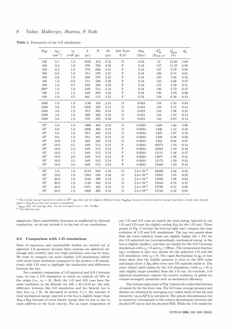
Table 1. Parameters of our 3-D simulations

NOB ng0 rcl L N δL Sim Type δtSN E‡inj η†mech η†O(cm−3) (×102 pc) (pc) (pc) F/O (Myr) (ESN ,51) (%)

100 0.1 1.0 1038 410 2.54 O 0.24 12 12.66 1.00100 0.3 1.0 876 700 2.50 F 0.24 137 11.37 0.98

100 0.5 1.0 779 620 2.51 F 0.24 137 8.70 0.69

100 0.8 1.0 714 570 2.51 F 0.24 136 6.74 0.61100 2.0 1.0 698 570 2.45 F 0.24 135 3.28 0.22

100 1.0 0.0 714 580 2.46 F 0.24 123 4.66 0.37100 1.0 0.7 649 300 4.33 F 0.24 131 4.49 0.41

100? 1.0 1.0 649 512 2.54 F 0.24 136 5.72 0.47

100 1.0 1.5 649 300 4.33 F 0.24 130 3.93 0.36100 1.0 0.3 601 512 2.35 F 0.24 138 6.38 0.44

1000 1.0 1.0 1136 450 2.54 O 0.024 134 5.34 0.941000 2.0 1.0 1055 420 2.51 O 0.024 134 3.17 0.44

1000 3.0 1.0 974 385 2.54 O 0.024 134 1.96 0.21

1000 4.0 1.0 909 360 2.54 O 0.024 134 1.25 0.141000 5.0 1.0 876 350 2.50 O 0.024 133 0.83 0.12

104 5.0 1.0 1006 400 2.52 O 0.0024 1408 1.80 0.86

104 6.0 1.0 1006 400 2.52 O 0.0024 1406 1.44 0.58

104 8.0 1.0 974 385 2.54 O 0.0024 1405 1.07 0.16

104 9.0 1.0 974 385 2.54 O 0.0024 1398 0.38 0.08

104 10.0 1.0 860 340 2.54 O 0.0024 1404 0.68 0.07

104 10.0 0.5 649 512 2.54 F 0.0024 16274 1.45 0.44

104 10.0 1.0 649 512 2.54 F 0.0024 16385 1.49 0.48

104 10.0 1.5 649 512 2.54 F 0.0024 15151 1.48 0.47

104 10.0 2.0 649 512 2.54 F 0.0024 13971 1.38 0.45

104 10.0 2.5 649 512 2.54 F 0.0024 13173 1.29 0.43

104 10.0 3.0 649 512 2.54 F 0.0024 12409 1.23 0.44

105 1.0 1.0 2110 850 2.48 O 2.4 × 10−4 16036 4.58 0.92

105 10.0 1.0 1363 550 2.48 O 2.4 × 10−4 15955 1.65 0.92

105 20.0 1.0 1233 490 2.52 O 2.4 × 10−4 15899 1.06 0.83

105 30.0 1.0 1136 450 2.54 O 2.4 × 10−4 15843 0.78 0.47

105 40.0 1.0 1071 425 2.52 O 2.4 × 10−4 15786 0.57 0.09

105 50.0 1.0 1006 400 2.52 O 2.4 × 10−4 15732 0.42 0.05

‡ The actual energy injected in units of 1051 erg; this can be slightly different from NOBESN because of extra kinetic energy injection; octant runs should

inject ≈ ESN/8 as only one octant is simulated.† ηmech (Eq. 19) and ηO (Eq. 13) are averaged over t = 29 − 30 Myr.? The fiducial run.

signatures. Since superbubble dynamics is unaffected by thermal

conduction, we do not include it in the rest of our simulations.

3.3 Comparison with 1-D simulations

Most of supernova and superbubble studies are carried out in

spherical 1-D geometry because these systems are spherical (al-though only crudely) and very high resolution runs can be done.We want to compare our more realistic 3-D simulations (albeit

with much lower resolution compared to the modern 1-D simula-tions) with 1-D runs to highlight the similarities and differences

between the two.

For a realistic comparison of 1-D spherical and 3-D Cartesianruns, we run a 3-D simulation in which we explode all SNe at

the origin (i.e., rcl = 0). Both the 1-D and 3-D runs have the

same resolution as the fiducial run (δL = δr=2.54 pc; the onlydifference between this 3-D simulation and the fiducial run is

that here rcl = 0). As discussed in section 3.1.1, the amount of

total mechanical energy injected in the box is slightly larger thanNOB × ESN because of extra kinetic energy that we put in due to

mass addition at the local velocity. For an exact comparison of

our 1-D and 3-D runs we match the total energy injected in our

1-D and 3-D runs (by slightly scaling ESN for the 1-D run). Three

panels of Fig. 9 (except the bottom-right one) compare the timeevolution of 1-D and 3-D simulations. The top two panels show

that the total radiative losses are slightly higher (by ≈ 3%) for

the 1-D spherical run (correspondingly, mechanical energy in thebox is slightly smaller), and they are similar for the 3-D Cartesian

simulations with rcl = 0 and rcl = 100 pc. The overpressure fraction(ηO) evolution is also very similar for the spherical 1-D and the

3-D simulation with rcl = 0. The rapid fluctuations in ηO at late

times show that the bubble pressure is close to the ISM valueand jumps above 1.5p0 after every new SN explodes inside it. Theouter (inner) shell radius for the 3-D simulation (with rcl = 0) is

only slightly larger (smaller) than the 1-D run. To conclude, 1-Dspherical simulations capture the correct evolution of global (or

volume-averaged) quantities such as mechanical efficiency.

The bottom right panel of Fig. 9 shows the radial distributionof emissivity for the three runs. For 3-D runs, average pressure and

density are obtained by averaging over radial shells of size δL and

emissivity (neniΛ[T ]) is calculated. The almost discontinuous risein emissivity corresponds to the contact discontinuity between the

shocked SN ejecta and the shocked ISM. While the 1-D emissivity

MNRAS 000, 000–000 (0000)


0.0

0.5

1.0

1.5

2.0

2.5

3.0

3.5

4.0

n/n

g0

1.27 Myr

3.18 Myr

4.78 Myr

9.55 Myr

14.33 Myr

20.70 Myr

10-2

10-1

100

101

102

103

p/p

0

−400 −300 −200 −100 0 100 200 300 400

x [pc]

−300

−200

−100

0

100

200

300

vx/c

0

100 150 200 250 300 350 400-2

-1

0

1

2

Figure 6. Gas density, pressure and x− velocity profiles along thex−axis (y = z = 0) for the fiducial run at various times. The swept-

up shell density decreases with time as the superbubble weakens

and eventually the shell propagates at the sound speed in theambient medium (c0 ≈ 15 km s−1). As seen in Fig. 1, the bubble

density is ∼ 4 orders of magnitude smaller than the ambient value.The main bubble pressure decreases with time, except during SN

injection, during which a high pressure core and an adiabatic

wind with large velocity and small pressure (similar to Chevalier& Clegg 1985) forms (the streaks seen in some panels of Fig. 5

are also a signature of this). The inset in the lowest panel shows

that the dense shell propagates at about half the sound speed inthe ambient ISM, but the velocities in the low density bubble aremuch higher.

profile is very sharp, the transition for 3-D runs (particularly withrcl = 100 pc) is smoother. This smoothing is due to deviation from

sphericity, in particular the crinkling of the contact surface seen in

the bottom panels of Fig. 1. This also makes the shell in Cartesiansimulations slightly thicker compared to the spherical 1-D run.

Radiative losses for 3-D runs are spread almost throughout theshell but are confined to the outer radiative relaxation layer inthe spherical run (see Fig. 5 in SRNS14).

Both the 1-D and 3-D simulations show that the bubbles aresmaller than the analytic estimates because of radiative cooling.Even in a uniform medium the shell can be unstable to various

3-D instabilities such as ‘Vishniac instability’ (Vishniac 1983),which affect the morphology of supershells (c.f. Fig. 13; see also

Krause et al. 2013).

3.4 Effects of cluster & ISM properties

After discussing the fiducial run in detail, in this section we studythe influence of cluster and ISM parameters (cluster radius rcl,number of OB stars NOB, and ISM density ng0).

0 5 10 15 20 25 30

time (Myr)

0.0

0.2

0.4

0.6

0.8

1.0

overp

ress

ure

fra

ctio

n(η

O)

ηO

0

1

2

3

4

5

6

7

rad

ius

(10

2p

c)

cluster radius

fizzli

ng

sta

rts

vO ≈ 16 km s-1

vI ≈ 08 km s-1

c0 ≈ 15 km s-1

outer boundary, RO

inner boundary, RI

Figure 7. The inner (green line) and outer (red line) radius of the

superbubble shell as a function of time for the fiducial run. Theblue line shows the overpressure fraction (ηO) as a function of

time. The superbubble starts to fizzle out when the overpressure

fraction starts falling from ≈ 1, which happens around 15 Myr.The average outer shell velocity is comparable to the ISM sound

speed; the inner shell speed is smaller. The bottom panel of Fig.

6 shows that at late times the shell material moves at ≈ c0/2,similar to the inner shell speed. The outer shell velocity is higher,

≈ c0, consistent with the shell density decreasing in time.

3.4.1 Effects of ISM density

The gas density in which SNe explode is a crucial parameter

that determines their subsequent evolution, both in adiabatic(rsb ∝ ρ−1/5) and radiative (radiative losses are higher for a larger

density) regimes. The left panel of Fig. 10 shows that the overpres-

sure fraction at early times (< 5 Myr) both falls and rises slowlyfor a higher density ISM. The overlap of SNe at higher densities

takes longer because the individual bubble radius is smaller for a

higher density and one needs to wait longer to fill the whole clus-ter with hot gas. At late times, the overpressure fraction drops

earlier for higher densities because of larger radiative losses (al-

though the bubble pressure scales as n3/5g0 according to Weaver

et al. 1977 adiabatic scaling).

The right panel of Fig. 10 shows that the bubble expandsmore rapidly in the lower density medium. It also shows that al-

though the shell in a higher density ISM expands slowly, it sweepsup more mass. An adiabatically expanding strong bubble in a

uniform medium is expected to sweep up gas at a rate ∝ n2/5g0 t

9/5.

Therefore, the ratio of mass swept by the shells with ng0 = 0.5, 0.8cm−3 shown in Fig. 10 is expected to be (0.5/0.8)2/5 ≈ 0.8, whereasthe actual value is ≈ 0.9. This is because the bubble expanding in

a denser ISM is slower than the adiabatic model due to radiative

losses; moreover, shells in a higher density medium suffer largerradiative losses. The shell for the highest density run (ng0 = 2cm−3) sweeps up an increasingly larger mass at later times be-cause RO ∝ c0t at late times, when the shell moves close to the

ISM sound speed.

MNRAS 000, 000–000 (0000)


0 50 100 150 200 250 300 350

x [pc]

0

50

100

150

200

250

300

350

y[p

c]

(a) No Thermal Conduction

0 50 100 150 200 250 300 350

x [pc]

(b) With Thermal Conduction

-4.0 -3.5 -3.0 -2.5 -2.0 -1.5 -1.0 -0.5 0.0 log10ng (cm-3)

Figure 8. A density contour plot and a quiver plot showing the projection of the velocity unit vector (3) in the x-y plane for the

fiducial simulation with (right panel) and without (left panel) conduction. Note that in the simulation with conduction there is a region≈ 100 − 150 pc in which the flow is directed inwards, whereas such a flow is absent in the run without conduction; this flow occurs as

conduction leads to evaporation of material from the shell into the bubble. The parameters of these runs are: number of SNe NOB = 100,

initial gas density ng0 = 1 cm−3, and cluster radius rcl = 100 pc. The snapshots are at ≈ 14.33 Myr.

3.4.2 Effects of cluster radius

The key difference of this work from SRNS14 is that we are doing

3-D simulations, which are necessary to study a realistic spatialdistribution of SNe. In 1-D spherical setup all SNe can only ex-

plode at the origin because of spherical symmetry. Fig. 11 showsthe evolution of overpressure volume fraction (ηO) as a function oftime for simulations with NOB = 104, ng0 = 10 cm−3, and different

star cluster radii.1 The plot has a characteristic shape with aninitial fall, a rise and saturation, and an eventual fall. The initial

fall occurs as isolated SNe, without overlapping, fizzle out due to

radiative losses (the top panels of Fig. 1 show density and pres-sure in this stage). The rise happens as SNe overlap and form a

superbubble. Eventually, the overpressure volume fraction dropsas the volume of the superbubble becomes too large and the outershock weakens due to adiabatic and radiative losses.

We can estimate the time when SNe start to overlap. The

radius of an isolated SN remnant is given by rSNR ∼ (ESNt2/ρ)1/5.

Suppose nt SNe have gone off independently by some time t.

The volume occupied by the non-overlapping SN remnants is∼ ∑nt

i=1(4π/3)(ESNi2δt2

SN/ρ)3/5 ∼ (4π/3)(ESNδt

2SN/ρ)

3/5 ∑nti=1 i

6/5 ∼(4π/3)(ESNδt

2SN/ρ)

3/5(5/11)(tNOB/τOB)11/5. Equating this volume

with the volume of the star cluster 4πr3cl/3 gives an estimate for

the time when SNe start to overlap (to,ad, estimate for SNR over-

lap assuming adiabatic evolution),

to,ad ∼ 0.16 Myr τ5/11OB,30N

−5/11OB,4 E

−3/11SN,51n

3/11g0,1r

15/11cl,2 , (14)

where ng0,1 is gas number density in units of 10 cm−3 and rcl,2 is

1 Here we choose parameters (NOB, ng0) different from the fiducial run

because the different stages of evolution are nicely separated in time for

this choice.The temporal behaviour is expected to be qualitatively similar

for different choice of parameters.

the radius of the star cluster in units of 100 pc. Note that we haveused Eq. 6 to obtain the above equation.

We can make another estimate for the SN overlap timescale

by assuming that SNe overlap only after they have become ra-diative. In this case, by a similar argument as that of the last

paragraph, the overlap time to,rad is given by τOB/NOB(rcl/rb,rad)3,

where rb,rad ∼ 37 pc E1/3SN,51n

−1/3g0 (Eq. 2 in Roy et al. 2013) is the

hot/dilute bubble radius when the remnant becomes radiative.Note that the bubble radius does not increase by more than a

factor of 2 after this time (e.g., Fig. 2 in Kim & Ostriker 2015).

Thus, the overlap time, assuming a radiative bubble, is given by

to,rad ∼ 0.6 Myr τOB,30N−1OB,4E

−1SN,51ng0,1r

3cl,2. (15)

The evolution seen in Fig. 11 lies somewhere in between Eqs. 14& 15.

The time for the overpressure volume to saturate after over-

lap of SNe and transition to a superbubble evolution is given by(using Weaver et al. 1977 scaling and setting the superbubbleshell radius equal to the cluster radius),

tsb ∼ 1.2 Myr r5/3cl,2N

−1/3OB,4η

−1/3mech,−1E

−1/3SN,51t

1/3OB,30n

1/3g0,1, (16)

where we have scaled the result with a mechanical efficiency ηmechof 0.1 (i.e., only ∼ 10% of the input SN energy goes into blowingthe superbubble; ∼ 90% is lost radiatively). This estimate for thetime of superbubble formation roughly matches the results in Fig.

11. Finally, the time when the superbubble pressure (∼ 0.75ρ32sb)

falls to ≈ 1.5 times the ISM pressure is given by (apart fromfactors of order unity, this is essentially the same as Eq. 12)

tfiz ∼ 10.3 Myr T−5/44 η

1/2mech,−1E

1/2SN,51τ

−1/2OB N

1/2OB,4n

−1/2g0,1, (17)

(T4 is the ISM temperature in units of 104 K) which is only slightly

lower than the time corresponding to the late time drop in theoverpressure volume fraction in Fig. 11. Note that unless the clus-

ter size (rcl) is unrealistically large, overlap of supernovae is likely

MNRAS 000, 000–000 (0000)


5 10 15 20 25 30

time (Myr)

0

1

2

3

4

5

6

7

8

kinetican

d∆

[thermal

energy

](105

1erg)

1D ∆ [thermal energy]

1D kinetic energy

3D ∆ [thermal energy]

3D kinetic energy

5 10 15 20 25 30

time (Myr)

0.0

0.2

0.4

0.6

0.8

1.0

overpressure

fraction

(ηO)

1D spherical

3D − rcl = 0 pc

3D − rcl = 100 pc

0 5 10 15 20

time (Myr)

0

1

2

3

4

5

6

7

radius(102

pc)

1D − RO

1D −RI

3D −RO, rcl = 0

3D − RI, rcl = 0

102

radius (pc)

10−30

10−29

10−28

10−27

10−26

10−25

10−24

10−23

10−22

neniΛ(T

),em

issivity(erg

cm−3

s−1)

1D spherical

3D − rcl = 0 pc

3D − rcl = 100 pc

0.0

0.2

0.4

0.6

0.8

1.0

1.2

1.4

radiative

losses

(105

3erg)

1D spherical

3D − rcl = 0 pc

3D − rcl = 100 pc

Figure 9. A comparison of 3-D (with rcl = 0 pc; rcl = 100 pc run is also shown for the right panels) and 1-D spherical simulations.

The top-left panel shows the kinetic and thermal energy added to the box by SNe. The top-right panel shows the overpressure fraction

(ηO ; solid lines) for the spherical 1-D run and the 3-D Cartesian runs with rcl = 0, 100 pc; also shown in lines connected by symbolsare cumulative radiative losses. The bottom-left panel shows the time evolution of the inner and outer shell radius for the 1-D and 3-D(rcl = 0) simulations. The bottom right panel shows the angle-averaged emissivity in the shell for the three simulations at 9.55 Myr

(corresponding to the bottom panels of Fig. 1). Note that there is a ‘gap’ in the emissivity for the 1-D spherical run in the dense shellwhere temperature is ≤ 104 K and we force Λ[T ] = 0.

to occur. In this state the time for a superbubble to fizzle out is

independent of the cluster size.

3.4.3 Effects of supernova rate: formation of a steadywind

Chevalier & Clegg 1985 found a solution (hereafter CC85) forthe wind driven by internal energy and mass deposited uniformlywithin an injection radius (r < R). This was applied to the galac-tic outflow in M82. For a large number of SNe (i.e., a large NOB),

MNRAS 000, 000–000 (0000)


5 10 15 20 25 30

time (Myr)

0.0

0.2

0.4

0.6

0.8

1.0

overp

ress

ure

fract

ion

(ηO)

3.0

Myr

5.0

Myr

9.5

Myr

15.0

Myr

20.0

Myr

0. 5

0. 8

2. 0

0 5 10 15 20 25 30

time (Myr)

0

1

2

3

4

5

6

rad

ius

(10

2p

c)cluster radius

0. 5, (RI + RO)/2

0. 8, (RI + RO)/2

2. 0, (RI + RO)/2

0

2

4

6

8

10

msh

(10

6M

sun)

msh

0. 5

0. 8

2. 0

Figure 10. The influence of ambient ISM density (ng0 = 0.5, 0.8, 2 cm−3) on the overpressure fraction (ηO ; left panel), and the inner

and outer shell radii (RI , RO) and the swept-up mass in the shell (msh; right panel) for NOB = 100 and rcl = 100 pc. The vertical lines in

the left panel mark the times when SNe overlap and produce an overpressured bubble and times when they fizzle out due to radiativeand adiabatic losses. The bubble expanding in the lower density medium expands faster and sweeps up smaller mass.

the mechanical energy injection can be approximated as a con-

stant luminosity wind, Lw = NOBESN/τOB. According to CC85,

within the injection radius (r . R) the mass density is constant,whereas at large radii (wind region, r & R) density is expected

to be ∝ r−2. A termination shock is expected at the radius where

the wind ram pressure balances the pressure inside the shockedISM. For small NOB, however, the individual SN ejecta does not

thermalize within the termination shock radius (rTS) as the SN

occurs inside a low density bubble (the bubble density is low inthe absence of significant mass loading as most of the ambient

gas is swept up in the outer shell) created by the previous SNe.For a large SN rate the solution should approach the steady state

described by Chevalier & Clegg 1985. SRNS14 derived analytic

constraints on NOB required for the existence of a smooth CC85wind inside the superbubble (see their Eq. 11) as,

δtSN,CC85 & 0.008 Myr E−9/26SN,51 t

4/13Myr n

−3/13g0 M

15/26SN,5�, (18)

where MSN,5� is the SN ejecta mass and tMyr is the age of the

starburst in Myr. This time between SNe corresponds to a re-quirement of NOB & 4×103 for a smooth CC85 wind to appear by

1 Myr. Using the standard stellar mass function, this corresponds

to a star formation rate of ∼ 0.01M�yr−1. This is a lower limit be-cause thermalization just before the termination shock does notlead to a high density/emissivity core, the characteristic feature

of a CC85 wind. Fig 12 shows the density profiles for a rangeof NOB (NOB = 105 corresponds to a SN rate of ∼ 0.003 yr−1).

As expected from thermalization of a SN within the ejecta of all

previous SNe (Eq. 18), a smooth CC85-type wind with density∝ r−2 at 30 Myr only forms for NOB & 104. Since SNe form in

OB associations, they are expected to overlap and form super-bubbles. For a sufficiently large number of SNe (& 105; e.g., in

the super star clusters powering a galactic wind in M82) a strong

termination shock (with Mach number � 1) exists till late times,which may accelerate majority of Galactic and extragalactic high

energy cosmic rays (e.g., Parizot et al. 2004). In contrast, strong

shocks (especially the reverse shock; McKee 1974) in isolated SNe

exist only at early times (. 103 yr), after which the reverse shock

crushes the central neutron star and the outer shock weakens withtime (in fact catastrophically after it becomes radiative). Fig. 13

shows the 2-D density snapshots of the 3-D runs shown in Fig. 12,

albeit at an earlier time. As expected, the shell is much thinnerfor a larger number of SNe. Also, a dense injection region and a

clear termination shock are visible for the runs with NOB & 104.

Crinkling of the contact discontinuity and the thin shell is thekey difference of 3-D runs as compared to the spherical 1-D sim-

ulations.

The SNe driven wind is able to maintain a strong non-radiative termination shock that is able to power the outwardmotion of the outer shock. The CC85 model has two parame-

ters: the efficiency with which star formation is converted intothermal energy (α ≡ ÛE/SFR), and the mass loading factor (β ≡ÛM/SFR), which determine the properties of galactic outflows (e.g.,

Sarkar et al. 2016). From our setup we can determine the mass-

loading for large NOB simulations by calculating the mass loss ratefrom the cluster measured at radii where the mass outflow rateÛM(r) ≡ 4πr2ρ3 is roughly constant. The mass loading factor for

our NOB = 105 run is ≈ 1 as most of the SN injected mass flows out

in a roughly steady wind. For much larger NOB (or equivalently,SFR) valid for starbursts, the mass loading factor can be reducedbecause of radiative cooling and mass drop-out from the dense

ejecta of SNe (e.g., Wunsch et al. 2007, 2008, 2011). Girichidiset al. 2016 have investigated launching of galactic outflows based

on multi-physics simulations which include variation in SN rate

and various strategies for placing supernovae (random, or at den-sity peaks or isolated). Pakmor et al. 2016; Simpson et al. 2016

investigate the effect of cosmic ray diffusion on dynamics of galac-tic outflows. We will investigate the effect of additional processes

in our future work.

MNRAS 000, 000–000 (0000)


0 5 10 15 20 25

time (Myr)

0.0

0.2

0.4

0.6

0.8

1.0

overp

ress

ure

fra

ctio

n(η

O)

00.5

Myr

01.5

Myr

04.2

Myr

07.5

Myr

11.5

Myr

15.0

Myr

NOB = 104

ng0 = 10 cm-3

rcl = 50 pc

rcl = 100 pc

rcl = 150 pc

rcl = 200 pc

rcl = 250 pc

rcl = 300 pc

Figure 11. The evolution of overpressure fraction as a function

of time for ng0 = 10 cm−3 and NOB = 104, but with different star-cluster sizes (rcl). The overpressure fraction plummets initially

as SNe are effectively isolated and cool catastrophically within 1

Myr. After that, as more SNe go off, they start to overlap andcreate an overpressured bubble. As expected, the transition to

overlap happens later for a larger star-cluster. The late time drop

in overpressure fraction, occurring due to adiabatic and radiativelosses, is similar for different rcl. This suggests that the superbub-

ble evolution is independent of the cluster size, once the coherent

overlap of SNe occurs.

4 DISCUSSION

In this section we discuss the astrophysical implications of our

work, focusing on radiative losses, comparison the observed HIsupershells, and gas expulsion from star clusters.

4.1 Mechanical efficiency & critical supernovarate for forming a superbubble

While isolated SNe lose all their energy by ∼ 1 Myr, even overlap-ping SNe forming superbubbles lose majority of energy injected

by SNe. The mechanical efficiency of superbubbles is defined as

ηmech ≡(KE + ∆TE)

Einj, (19)

where KE is the total kinetic energy of the box, ∆TE is the in-

crease in the box thermal energy, and Einj is the energy injectedby SNe (which is slightly larger than NOBESN because mass is

added at the local velocity). By energy conservation (the compu-

tational box is large enough that energy is not transported in toor out of it), ηmech = 1− RL/Einj, where RL are cumulative radia-tive losses. Fig. 14 shows the mechanical efficiency (Eq. 19) as afunction of the initial gas density (ng0) at various times for runswith different NOB. One immediately sees that mechanical effi-

ciency decreases with an increasing ISM density (ng0). Efficiencyalso decreases with time (by almost a factor of 10 from 5 to 30Myr), especially for higher densities. The maximum efficiency is

∼ 20%, occurring at early times. Our simulations show that themechanical efficiency of 3-D and 1-D simulations are comparable

and almost independent of the cluster size (rcl, see section 3.3 &

10-1

100

101

102

radius (pc)/(Einj, 51)1/5

10-5

10-4

10-3

10-2

10-1

100

101

102

nu

mb

er

den

sity

(cm

-3)

ρ ∝ r-2

ng0 = 1. 0 cm-3t = 30. 0 Myr;

CC85 wind solution

shock

edw

ind

term

ina

tion

shock

shocked ISM (thin shell)

ISM

105

-1D

102

-3D

103

-3D

104

-3D

105

-3D

Figure 12. Spherically averaged gas density profiles for 3-D runs

at 30 Myr (rcl = 100 pc, except for the 1-D spherical run; ng0 = 1cm−3) with various NOB. Radius has been scaled with the ex-

pected scaling ( E1/5inj,51 ≈ N

1/5OB is the total mechanical energy in-

jected in units of 1051 erg; see Table 1). The thin vertical lines

mark the cluster radius (rcl) in the scaled unit. The density pro-

file attains a smooth, steady CC85 profile (its signature is theρ ∝ r−2 profile beyond a core region) within the bubble for a large

NOB & 104, consistent with the analytic considerations in section

4.3 of SRNS14 (see also Fig. 3 in their paper). The radiative shellin 1-D run (with the same resolution as the 3-D run) is much

thinner as compared to 3-D because the 3-D shell is not perfectlyspherical and the contact discontinuity is crinkled (see Fig. 13).

The outer shock is weaker for a smaller NOB but its location scales

with the analytic scaling (∝ N1/5OB ).

Fig. 9), provided that SNe overlap before fizzling out. A rough

scaling of ηmech ∝ n−2/3g0 , valid at most times, can be deduced from

Fig. 14. Also note that the mechanical efficiency increases veryslightly for a larger number of SNe.

Fig. 14 shows mechanical efficiencies that are about an orderof magnitude smaller than the values quoted in SRNS14. For ex-ample, the efficiency (which equals 1− fractional radiative losses;see the right panel of Fig. 8 in SRNS14) for NOB = 105 and ng0 = 1cm−3 in SRNS14 at 30 Myr is ≈ 40%. The value for the same choiceof parameters from Fig. 14 is ≈ 6%, smaller by a factor of ≈ 7.

This discrepancy is mainly due to the much higher resolution inthe 1-D simulations of SRNS14 (see section 4.4).

Fig. 11 shows that the overpressure volume fraction ηO forng0 = 10 cm−3 and NOB = 104 has a similar value for cluster

sizes as large as rcl = 300 pc. This means that the evolution ofthe superbubble is independent of rcl, as long as overlap of SNe

happens before the cluster age, which is very likely not only forindividual star clusters but also for clusters of star clusters asin the center of M82 galaxy (O’Connell et al. 1995). Therefore,the key parameter that determines if the superbubble remains

sufficiently overpressured by the end of the star-cluster lifetime,for a given gas density, is the number of SNe NOB (and not thecluster size rcl).

The overpressure volume fraction (defined in Eq. 13) is anappropriate diagnostic to determine if a superbubble has fizzled

MNRAS 000, 000–000 (0000)


0

20

40

60

80

100

120

140

y[p

c]/(

Ein

j,51)1

/5

NOB = 102

NOB = 103

−140−120−100 −80 −60 −40 −20 0

x[pc]/(Einj, 51)1/5

−140

−120

−100

−80

−60

−40

−20

0

y[p

c]/(

Ein

j,51)1

/5

NOB = 104

0 20 40 60 80 100 120 140

x[pc]/(Einj, 51)1/5

NOB = 105

-4.8 -4.0 -3.2 -2.4 -1.6 -0.8 0.0 0.8 log10ng (cm-3)

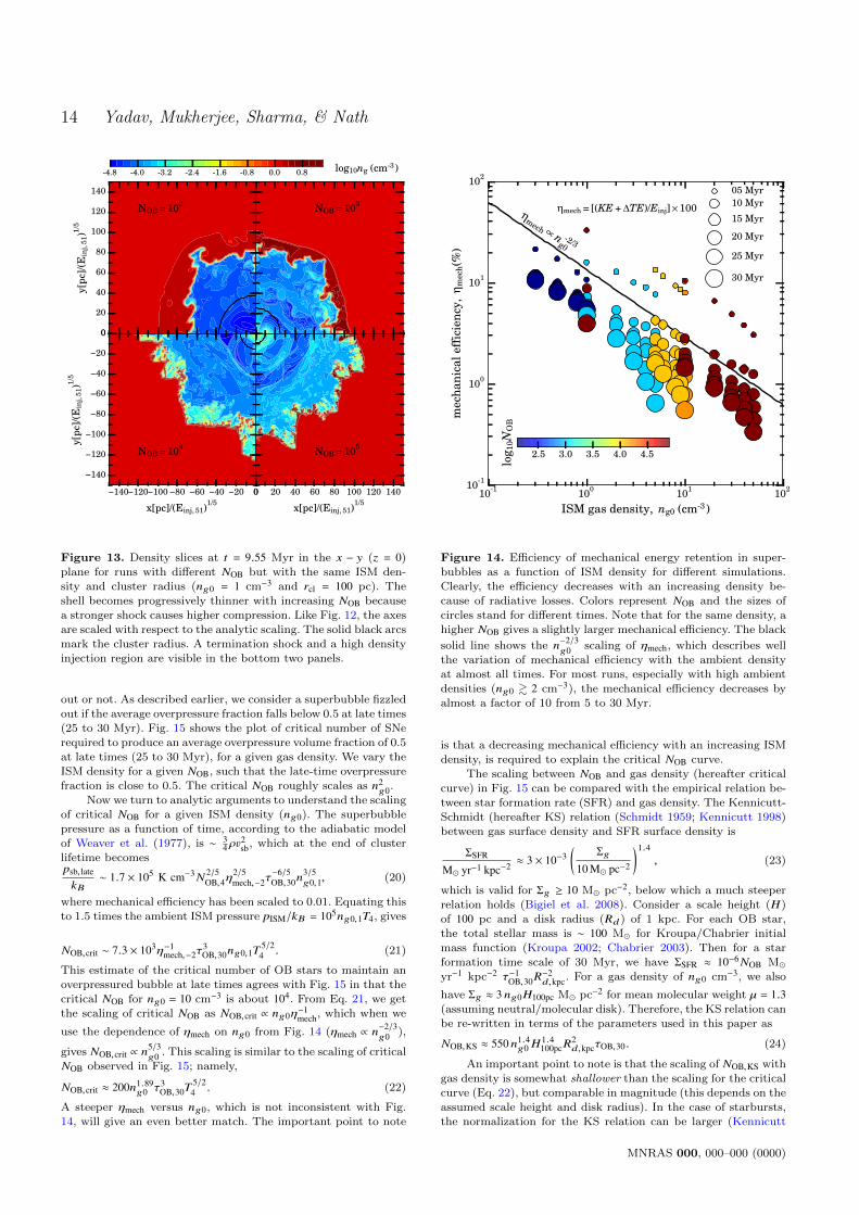
Figure 13. Density slices at t = 9.55 Myr in the x − y (z = 0)plane for runs with different NOB but with the same ISM den-

sity and cluster radius (ng0 = 1 cm−3 and rcl = 100 pc). The

shell becomes progressively thinner with increasing NOB becausea stronger shock causes higher compression. Like Fig. 12, the axes

are scaled with respect to the analytic scaling. The solid black arcs

mark the cluster radius. A termination shock and a high densityinjection region are visible in the bottom two panels.

out or not. As described earlier, we consider a superbubble fizzled

out if the average overpressure fraction falls below 0.5 at late times

(25 to 30 Myr). Fig. 15 shows the plot of critical number of SNerequired to produce an average overpressure volume fraction of 0.5

at late times (25 to 30 Myr), for a given gas density. We vary the

ISM density for a given NOB, such that the late-time overpressurefraction is close to 0.5. The critical NOB roughly scales as n2

g0.

Now we turn to analytic arguments to understand the scaling

of critical NOB for a given ISM density (ng0). The superbubblepressure as a function of time, according to the adiabatic model

of Weaver et al. (1977), is ∼ 34ρ3

2sb, which at the end of cluster

lifetime becomespsb, latekB

∼ 1.7 × 105 K cm−3N2/5OB,4η

2/5mech,−2τ

−6/5OB,30n

3/5g0,1, (20)

where mechanical efficiency has been scaled to 0.01. Equating thisto 1.5 times the ambient ISM pressure pISM/kB = 105ng0,1T4, gives

NOB,crit ∼ 7.3 × 103η−1mech,−2τ

3OB,30ng0,1T

5/24 . (21)

This estimate of the critical number of OB stars to maintain anoverpressured bubble at late times agrees with Fig. 15 in that the

critical NOB for ng0 = 10 cm−3 is about 104. From Eq. 21, we get

the scaling of critical NOB as NOB,crit ∝ ng0η−1mech, which when we

use the dependence of ηmech on ng0 from Fig. 14 (ηmech ∝ n−2/3g0 ),

gives NOB,crit ∝ n5/3g0 . This scaling is similar to the scaling of critical

NOB observed in Fig. 15; namely,

NOB,crit ≈ 200n1.89g0 τ3

OB,30T5/2

4 . (22)

A steeper ηmech versus ng0, which is not inconsistent with Fig.

14, will give an even better match. The important point to note

10-1

100

101

102

ISM gas density, ng0 (cm-3)

10-1

100

101

102

mech

an

ica

leff

icie

ncy

,η

mech

(%)

05 Myr

10 Myr

15 Myr

20 Myr

25 Myr

30 Myr

ηmech = [(KE + ∆TE)/Einj] × 100η

mech ∝

n -2/3g0

2.5 3.0 3.5 4.0 4.5

log

10N

OB

Figure 14. Efficiency of mechanical energy retention in super-bubbles as a function of ISM density for different simulations.

Clearly, the efficiency decreases with an increasing density be-

cause of radiative losses. Colors represent NOB and the sizes ofcircles stand for different times. Note that for the same density, a

higher NOB gives a slightly larger mechanical efficiency. The black

solid line shows the n−2/3g0 scaling of ηmech, which describes well

the variation of mechanical efficiency with the ambient density

at almost all times. For most runs, especially with high ambientdensities (ng0 & 2 cm−3), the mechanical efficiency decreases by

almost a factor of 10 from 5 to 30 Myr.

is that a decreasing mechanical efficiency with an increasing ISM

density, is required to explain the critical NOB curve.

The scaling between NOB and gas density (hereafter criticalcurve) in Fig. 15 can be compared with the empirical relation be-

tween star formation rate (SFR) and gas density. The Kennicutt-

Schmidt (hereafter KS) relation (Schmidt 1959; Kennicutt 1998)between gas surface density and SFR surface density is

ΣSFR

M� yr−1 kpc−2 ≈ 3 × 10−3(

Σg

10 M� pc−2

)1.4, (23)

which is valid for Σg ≥ 10 M� pc−2, below which a much steeper

relation holds (Bigiel et al. 2008). Consider a scale height (H)

of 100 pc and a disk radius (Rd) of 1 kpc. For each OB star,the total stellar mass is ∼ 100 M� for Kroupa/Chabrier initial

mass function (Kroupa 2002; Chabrier 2003). Then for a star

formation time scale of 30 Myr, we have ΣSFR ≈ 10−6NOB M�yr−1 kpc−2 τ−1

OB,30R−2d,kpc. For a gas density of ng0 cm−3, we also

have Σg ≈ 3 ng0H100pc M� pc−2 for mean molecular weight µ = 1.3(assuming neutral/molecular disk). Therefore, the KS relation canbe re-written in terms of the parameters used in this paper as

NOB,KS ≈ 550 n1.4g0 H

1.4100pcR

2d,kpcτOB,30. (24)

An important point to note is that the scaling of NOB,KS withgas density is somewhat shallower than the scaling for the critical

curve (Eq. 22), but comparable in magnitude (this depends on theassumed scale height and disk radius). In the case of starbursts,

the normalization for the KS relation can be larger (Kennicutt

MNRAS 000, 000–000 (0000)


10-1

100

101

102

ISM gas density, ng0 (cm-3)

101

102

103

104

105

106

nu

mb

er

of

sup

ern

ova

e,

NO

B

NOB ∼ 102. 33 + /-0. 15

n1. 89 + /-0. 18g0

ηO-0. 5

ηO < 0. 5

ηO > 0. 5

-0.5 -0.3 -0.1 +0.1 +0.3

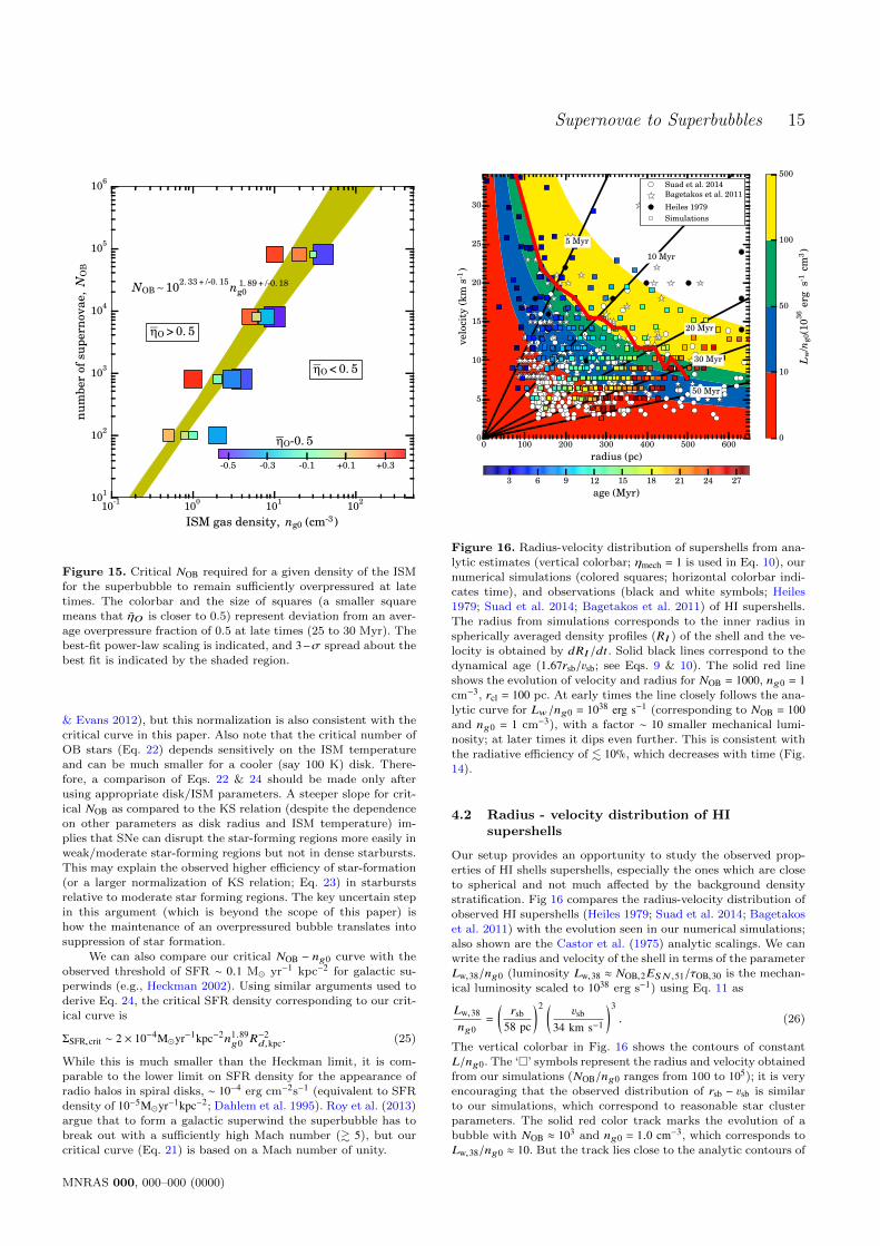
Figure 15. Critical NOB required for a given density of the ISMfor the superbubble to remain sufficiently overpressured at late

times. The colorbar and the size of squares (a smaller square

means that ηO is closer to 0.5) represent deviation from an aver-age overpressure fraction of 0.5 at late times (25 to 30 Myr). The

best-fit power-law scaling is indicated, and 3−σ spread about the

best fit is indicated by the shaded region.

& Evans 2012), but this normalization is also consistent with thecritical curve in this paper. Also note that the critical number of

OB stars (Eq. 22) depends sensitively on the ISM temperature

and can be much smaller for a cooler (say 100 K) disk. There-fore, a comparison of Eqs. 22 & 24 should be made only after

using appropriate disk/ISM parameters. A steeper slope for crit-

ical NOB as compared to the KS relation (despite the dependenceon other parameters as disk radius and ISM temperature) im-

plies that SNe can disrupt the star-forming regions more easily inweak/moderate star-forming regions but not in dense starbursts.

This may explain the observed higher efficiency of star-formation

(or a larger normalization of KS relation; Eq. 23) in starburstsrelative to moderate star forming regions. The key uncertain step

in this argument (which is beyond the scope of this paper) ishow the maintenance of an overpressured bubble translates intosuppression of star formation.

We can also compare our critical NOB − ng0 curve with the

observed threshold of SFR ∼ 0.1 M� yr−1 kpc−2 for galactic su-

perwinds (e.g., Heckman 2002). Using similar arguments used toderive Eq. 24, the critical SFR density corresponding to our crit-

ical curve is

ΣSFR,crit ∼ 2 × 10−4M�yr−1kpc−2n1.89g0 R−2

d,kpc. (25)

While this is much smaller than the Heckman limit, it is com-

parable to the lower limit on SFR density for the appearance of

radio halos in spiral disks, ∼ 10−4 erg cm−2s−1 (equivalent to SFRdensity of 10−5M�yr−1kpc−2; Dahlem et al. 1995). Roy et al. (2013)

argue that to form a galactic superwind the superbubble has tobreak out with a sufficiently high Mach number (& 5), but our

critical curve (Eq. 21) is based on a Mach number of unity.

0 100 200 300 400 500 600

radius (pc)

0

5

10

15

20

25

30

velo

city

(km

s-1)

Suad et al. 2014

Bagetakos et al. 2011

Heiles 1979

Simulations

5 Myr

10 Myr

20 Myr

30 Myr

50 Myr

0

10

50

100

500

Lw/n

g0(1

036

erg

s-1cm

3)

3 6 9 12 15 18 21 24 27

age (Myr)

Figure 16. Radius-velocity distribution of supershells from ana-

lytic estimates (vertical colorbar; ηmech = 1 is used in Eq. 10), ournumerical simulations (colored squares; horizontal colorbar indi-

cates time), and observations (black and white symbols; Heiles1979; Suad et al. 2014; Bagetakos et al. 2011) of HI supershells.

The radius from simulations corresponds to the inner radius in

spherically averaged density profiles (RI ) of the shell and the ve-locity is obtained by dRI /dt. Solid black lines correspond to the

dynamical age (1.67rsb/3sb; see Eqs. 9 & 10). The solid red line

shows the evolution of velocity and radius for NOB = 1000, ng0 = 1cm−3, rcl = 100 pc. At early times the line closely follows the ana-

lytic curve for Lw/ng0 = 1038 erg s−1 (corresponding to NOB = 100and ng0 = 1 cm−3), with a factor ∼ 10 smaller mechanical lumi-nosity; at later times it dips even further. This is consistent with

the radiative efficiency of . 10%, which decreases with time (Fig.

14).

4.2 Radius - velocity distribution of HIsupershells

Our setup provides an opportunity to study the observed prop-

erties of HI shells supershells, especially the ones which are closeto spherical and not much affected by the background density

stratification. Fig 16 compares the radius-velocity distribution ofobserved HI supershells (Heiles 1979; Suad et al. 2014; Bagetakoset al. 2011) with the evolution seen in our numerical simulations;also shown are the Castor et al. (1975) analytic scalings. We can

write the radius and velocity of the shell in terms of the parameterLw,38/ng0 (luminosity Lw,38 ≈ NOB,2ESN ,51/τOB,30 is the mechan-

ical luminosity scaled to 1038 erg s−1) using Eq. 11 as

Lw,38ng0

=

(rsb

58 pc

)2 (3sb

34 km s−1

)3. (26)

The vertical colorbar in Fig. 16 shows the contours of constant

L/ng0. The ‘�’ symbols represent the radius and velocity obtained

from our simulations (NOB/ng0 ranges from 100 to 105); it is veryencouraging that the observed distribution of rsb − 3sb is similar

to our simulations, which correspond to reasonable star cluster

parameters. The solid red color track marks the evolution of abubble with NOB ≈ 103 and ng0 = 1.0 cm−3, which corresponds to

Lw,38/ng0 ≈ 10. But the track lies close to the analytic contours of

MNRAS 000, 000–000 (0000)


Lw,38/ng0 ≈ 0.5 − 1.0. It means that, for a given rsb − vsb the adia-

batic theory overestimates Lw,38/ng0 by a factor of ∼ 10−20. This

discrepancy is primarily due to large radiative losses; mechanicalefficiency in Fig. 14 . 10% is consistent with the evolution in the

rsb − 3sb space. Also we note that some of the simulation points

(below the t = 30 Myr line) have a dynamical age (≡ 5rsb/3vsb)longer than the simulation time.

If SNe are the dominant cause of bubble formation, then

we require large OB associations for the creation of the observedHI supershells. In order to quantify the size of OB associations,

we also need to evaluate the mechanical energy injection from

stellar winds and radiation. However, even without accounting forthese additional energy/momentum sources, the observed shells

are much smaller and slower compared to what is expected fromthe predictions of adiabatic theory applied to the observed stellar

population – the so-called power problem in superbubbles (Oey

2009 and references therein). Our simulations show that radiativelosses can account for the power problem.

4.3 Gas removal from clusters

Due to the presence of feedback from OB stars (radiative, stellar

winds and SNe) the star forming regions clear gas on timescales∼ 106 yr (Lada & Lada 2003). For clusters simulated by us the

mstars/mcl ∼ 0.17NOB,2/ng0r3cl,100 < 1 (for each OB star, the total

stellar mass is ∼ 100 M� for Kroupa/Chabrier initial mass func-

tion), therefore the gravitational well is largely provided by the

cluster gas (this is also true for embedded clusters buried in theirnatal molecular clumps). As a result of gas expulsion the cluster

potential becomes shallower and the cluster may become unbound

depending on the ratio of gas removal timescale and dynamicaltimescale of the cluster (Lada & Lada 2003). If the gas expulsion

time is long compared to the dynamical time, the stars can adi-

abatically attain new viral equilibrium without being unbound.However, in the opposite regime because of a suddenly reduced

gravity majority of stars become unbound. The timescale of gas

expulsion is also important to account for multiple populationsobserved in globular clusters (e.g., Krause et al. 2016 and refer-

ences therein).

While our simulations do not account for gravity that holdsthe star cluster together (inclusion of gravity is important for

strongly bound massive clouds, not so much for smaller clumps

with lower gravitational binding energies), we can qualitativelyunderstand the action of supernova/stellar wind energy injection

in gas expulsion from star clusters. Fig. 17 shows the mass fractionmcl(t)/mcl(0) (mcl is the gas mass inside the cluster radius, r < rcl)as a function of time for various values of NOB and ng0. Since

the ratio of energy injected by SNe to the gravitational potentialenergy ∼ NOBESN/(Gµ2m2

pn2g0r

5cl) ∼ 5 × 105NOB,2ESN,51/(n2

g0r5cl,2)

is large, the effect of neglecting gravity is negligible for the choice

of our parameters (for simulations with gravity, see Calura et al.2015; Krause et al. 2016). We find that the clusters are evac-

uated due to the formation of a superbubble within . 10 Myr(Fig. 17). As expected, lower ISM density and higher NOB evac-uate the cluster gas in a shorter time. An estimate of evacuation

timescale is given in Eq. 16. The estimate depends strongly on thecluster radius (rcl) but is weakly sensitive to parameters such asISM density, NOB, ηmech, etc. The results in Fig. 17 are consistent

with the timescale in Eq. 16; therefore, for different parametersour numerical results can be scaled according to the theoretical

scaling.

4.4 Convergence of ηmech & temperaturedistribution of radiative losses

One of the key questions is whether our results are converged.Convergence of the fiducial 3-D simulation is discussed in Ap-

pendix B. Fig. B1 clearly shows that the higher resolution simula-

tions show finer features. What about the convergence of volume-

averaged quantities such as mechanical efficiency (ηmech)? Fig. 18shows mechanical efficiency (Eq. 19) measured at 30 Myr for the

fiducial 3-D and 1-D runs at various resolutions. Even average

quantities like ηmech do not show perfect convergence (we get ahigher value of ηmech with increasing resolution). The 1-D simula-

tions can be carried out at a much higher resolution than the 3-D

ones, and yet ηmech increases with an increasing resolution. In sec-tion 3.3 we show that at the same resolution the radiative losses

are comparable in 3-D and 1-D (top-right panel of Fig. 9). From

this, we expect that even the very high resolution 3-D simula-tions (which are beyond the capabilities of current computational

resources) will not show convergence.

Recent very high resolution 1-D simulations (Gentry et al.2016; Gupta et al. 2016) have highlighted the importance of very

high resolution to obtain mechanical efficiency and momentumdelivered to the ISM by supernovae. However, our Fig. 18 clearly

shows the lack of convergence even at the highest resolutions. The

cooling losses in any simulation with unresolved boundary layers(radiative relaxation layer and contact discontinuity) will keep

on decreasing with an increasing resolution because the volume

of cooling layers (and hence radiative loss rate) decreases with anincreasing resolution. This means that convergence can only be

achieved by explicitly including diffusive processes such as ther-

mal conduction and/or viscosity, which can numerically resolvethe radiative layers. Moreover, the values of physical conductiv-

ity and viscosity are too small (especially for the dense phases)

to be resolved on the grid. Therefore, artificially large numeri-cal diffusivities (which may crudely mimic small-scale turbulent

transport) must be used. The importance of resolving coolinglayers via explicit thermal conduction to obtain convergence in

thermal instability simulations is highlighted in Koyama & In-

utsuka (2004). Similarly Fromang & Papaloizou (2007); Lesur &Longaretti (2007) show that explicit resistivity and viscosity are

required to get converged results for angular momentum trans-

port due to magnetorotational instability (MRI) in unstratifiedshearing boxes.

One observationally important diagnostic is the temperature

distribution of cooling losses in superbubbles; this determines thewavebands in which they emit. Fig. 19 shows the temperature

distribution of the radiative loss rate for the fiducial 3-D run

with and without thermal conduction. Both with and withoutconduction, the radiative losses occur primarily at ∼ 104 K; the

fractional radiative losses for T < 105 K are 99.6% and 99.3% with

and without conduction, respectively. This result is consistentwith the recent superbubble simulations in dense molecular gas

(Gupta et al. 2016), which show that the cooling losses at ∼ 104 Kare about two order of magnitude larger than X-ray (∼ 106−7 K)

and molecular (∼ 100 K) losses. Thermal conduction reduces the

maximum temperature in the hot bubble due to the evaporationof mass from the dense shell to the hot bubble, as shown in Fig. 8.

5 CONCLUSIONS

We have carried out 3-D hydrodynamic simulations of supernovae

(SNe) in an OB association that creates and drives a superbubble.Our aim has been to study the effect of multiple SNe distributed

over a limited region of a cluster, on the ambient material faroutside the cluster, and derive the dependence of fundamental

parameters such as the efficiency of energy deposition and thecritical number of SN required to create overpressured bubbles.Our settings have been admittedly, and intentionally, kept ide-

alized so that we can perform controlled numerical experiments.Physical effects such as magnetic fields, thermal conduction, strat-ification, and inhomogeneities in the ambient gas, which we have

MNRAS 000, 000–000 (0000)


0 2 4 6 80.0

0.2

0.4

0.6

0.8

1.0

ma

ssfr

act

ion

[mcl(t

)/m

cl(0

)]

NOB = 102

ng0

0. 2

0. 3

0. 5

0. 8

1. 0

2 4 6 8

NOB = 103

ng0

1. 0

2. 0

3. 0

4. 0

5. 0

1 2 3 4

NOB = 104

ng0

5. 0

6. 0

8. 0

9. 0

10. 0

1 2 3 4

NOB = 105

ng0

10

20

30

40

50

time (Myr)

Figure 17. The fraction of original cluster gas remaining within the cluster (r < rcl; rcl = 100 pc for all these runs) as a function of time

for various SN counts (NOB). Each of the sub-panels show curves corresponding to different values of gas density ng0, the initial ISMdensity inside the cluster. It is noted that even a small NOB makes the cluster lose all its gas by about 8 − 10 Myr. The evacuation time

increases with density, as expected.

10-2

10-1

100

101

grid resolution (pc)

100

101

102

mech

an

ica

leff

icie

ncy

,η

mech

(%)

y = axb , a = 8. 54, b = -0. 44

1D-simulations

3D-simulations

0 5 10 15 20 25 30

time(Myr)

0

10

20

30

40

50

60

mech

an

ica

leff

icie

ncy

,η

mech

(%)

2. 500 pc

0. 250 pc

0. 050 pc

0. 025 pc

Figure 18. Mechanical efficiency measured at 30 Myr as a func-tion of grid resolution for various 1-D and 3-D superbubble sim-ulations. The grid parameters are NOB = 100, ng0 = 1 cm−3 andrcl = 0 (for 1-D runs) and rcl = 100 pc (for 3-D runs). The blue

solid line is the best least squares power-law fit to the data points.The inset shows the evolution of mechanical efficiency for the high

resolution 1-D runs. Mechanical efficiency does not converge evenfor the highest resolution 1-D simulations.

not included here, presumably do play important roles in super-

bubble formation and evolution, and will be the focus of our futurestudies.

The broad astrophysical implications of our results are dis-

cussed in section 4. Our key results can be summarized as follows:

• While isolated SNe fizzle out by ∼ 1 Myr due to radiation

losses, for a realistic cluster size it is likely that subsequent SNe

4 5 6 7 8 9

log10 Tg (K)

26

28

30

32

34

36

38

40

log

10

[dE

rad/d

tdT

](e

rgs-1

K-1

)

NC, 1. 27 Myr

NC, 4. 77 Myr

NC, 14. 33 Myr

TC, 1. 27 Myr

TC, 4. 77 Myr

TC, 14. 33 Myr

Figure 19. Radiative loss rate per temperature bin (dErad/dtdT )as a function of gas temperature at different times for our fiducialsimulation with (TC) and without (NC) thermal conduction. Wecalculate the radiative loss rates in logarithmically spaced tem-

perature bins with ∆ log10 T = 0.1. Thermal conduction reducesthe maximum gas temperature in the box because of evaporation

of matter into the hot bubble.

go off in a hot and tenuous medium and sustain a shock lasting for

the cluster lifetime ∼ 30 Myr, comparable to the galactic dynam-ical timescale. 1-D numerical simulations faithfully capture the

global energetics but cannot, by construction, capture morpho-logical features such as the crinkling of the contact discontinuityseen in 3-D.

• While most of the input energy is lost via radiative cool-

ing, the superbubble retains a fraction ηmech of the input energy,

MNRAS 000, 000–000 (0000)


and this fraction scales as ηmech ∝ n−2/3g0 , being of order ∼ 6% for

ng0 ∼ 1 cm−3 over a time period of ∼ 30 Myr. We note that the

mechanical efficiency increases with an increasing resolution, and

that converged result can only be obtained by resolving coolinglayers using explicit diffusion.

• We have explored the parameter space of ISM density (ng0),

number of SNe (NOB) and star cluster radius (rcl) to study the

conditions for the formation of an overpressured superbubble. Forrealistic cluster sizes, we find that the bubble remains overpres-

sured only if, for a given ng0, NOB is larger than a threshold

value. Our results show that threshold condition can be roughlyexpressed as NOB,crit ∼ 200n1.9

g0 , where ng0 is the particle density

in cm−3.

• Classical adiabatic superbubble evolution overestimates theratio of the wind luminosity and the ISM density (Lw/ng0) by a

factor of ∼ 10 − 20, by not taking radiation losses into account.

This explains the ‘power problem’ of the observed size and speedof superbubbles, and our simulations confirm that radiative losses

are the reason for discrepancies between the size-speed distribu-

tion of HI supershells and the sizes of OB associations drivingthem.

• We confirm that a minimum value of NOB(& 104) is need to

produce a steady wind and a strong termination shock within the

cluster region. For a smaller number of SNe, all the supernovaenergy is deposited at the radiative dense shell.

ACKNOWLEDGMENTS

We are grateful to the Supercomputing Education and ResearchCentre (SERC) at IISc for facilitating our use of Cray XC40-

SahasraT cluster, without which these challenging simulations

could not be carried out. This work is partly supported by theDST-India grant no. Sr/S2/HEP-048/2012 and an India-Israel

joint research grant (6-10/2014[IC]; which also supports Naveen

Yadav). We wish to thank Kartick Sarkar, Arpita Roy, DeovratPrasad, Prakriti Pal Choudhury and Prasun Dhang for many

helpful discussions. We thank Siddhartha Gupta for convincing

us to study the convergence of mechanical efficiency in 1-D.

REFERENCES

Alexiades V., Amiez G., Gremaud P.-A., 1996, Communications

in Numerical Methods in Engineering, 12, 31

Avedisova V. S., 1972, Soviet Ast., 15, 708Bagetakos I., Brinks E., Walter F., de Blok W. J. G., Usero A.,

Leroy A. K., Rich J. W., Kennicutt Jr. R. C., 2011, AJ, 141,23

Bigiel F., Leroy A., Walter F., Brinks E., de Blok W. J. G.,Madore B., Thornley M. D., 2008, AJ, 136, 2846

Calura F., Few C. G., Romano D., D’Ercole A., 2015, ApJ, 814,L14

Castor J., McCray R., Weaver R., 1975, ApJ, 200, L107Chabrier G., 2003, PASP, 115, 763

Chevalier R. A., Clegg A. W., 1985, Nature, 317, 44Chu Y.-H., Gruendl R. A., 2008, in Beuther H., Linz H., Henning

T., eds, Astronomical Society of the Pacific Conference Se-ries Vol. 387, Massive Star Formation: Observations Confront

Theory. p. 415 (arXiv:0712.1871)Courant R., Friedrichs K., Lewy H., 1928, Mathematische An-

nalen, 100, 32Cox D. P., 1972, ApJ, 178, 159Creasey P., Theuns T., Bower R. G., 2013, MNRAS, 429, 1922

Dahlem M., Lisenfeld U., Golla G., 1995, ApJ, 444, 119De Avillez M. A., Breitschwerdt D., 2005, A&A, 436, 585Durier F., Dalla Vecchia C., 2012, MNRAS, 419, 465

Efstathiou G., 2000, MNRAS, 317, 697

Ferrand G., Marcowith A., 2010, A&A, 510, A101

Fromang S., Papaloizou J., 2007, A&A, 476, 1113

Gatto A., et al., 2015, MNRAS, 449, 1057

Gentry E. S., Krumholz M. R., Dekel A., Madau P., 2016,

preprint, (arXiv:1606.01242)

Gies D. R., 1987, ApJS, 64, 545

Girichidis P., et al., 2016, MNRAS, 456, 3432

Gupta S., Nath B. B., Sharma P., Shchekinov Y., 2016, MNRAS,

462, 4532

Heckman T. M., 2002, in Mulchaey J. S., Stocke J. T., eds, As-tronomical Society of the Pacific Conference Series Vol. 254,

Extragalactic Gas at Low Redshift. p. 292 (arXiv:astro-

ph/0107438)

Heiles C., 1979, ApJ, 229, 533

Hennebelle P., Iffrig O., 2014, A&A, 570, A81

Joung M. K. R., Mac Low M.-M., 2006, ApJ, 653, 1266

Kauffmann G., et al., 2003, MNRAS, 341, 54

Kennicutt Jr. R. C., 1998, ApJ, 498, 541

Kennicutt R. C., Evans N. J., 2012, ARA&A, 50, 531

Kim C.-G., Ostriker E. C., 2015, ApJ, 802, 99

Koyama H., Inutsuka S.-i., 2004, ApJ, 602, L25

Krause M., Fierlinger K., Diehl R., Burkert A., Voss R., ZieglerU., 2013, A&A, 550, A49

Krause M., Diehl R., Bohringer H., Freyberg M., Lubos D., 2014,

A&A, 566, A94

Krause M. G. H., Charbonnel C., Bastian N., Diehl R., 2016,

A&A, 587, A53

Kroupa P., 2002, Science, 295, 82

Krumholz M. R., Tan J. C., 2007, ApJ, 654, 304

Krumholz M. R., et al., 2014, Protostars and Planets VI, pp 243–266

Lada C. J., Lada E. A., 2003, ARA&A, 41, 57

Larsen S. S., 1999, A&AS, 139, 393

Lesur G., Longaretti P.-Y., 2007, MNRAS, 378, 1471

Li M., Ostriker J. P., Cen R., Bryan G. L., Naab T., 2015, ApJ,

814, 4

Mac Low M.-M., Klessen R. S., 2004, Reviews of Modern Physics,

76, 125

Mac Low M.-M., McCray R., 1988, ApJ, 324, 776

Martizzi D., Faucher-Giguere C.-A., Quataert E., 2015, MNRAS,450, 504

McCammon D., Burrows D. N., Sanders W. T., Kraushaar W. L.,

1983, ApJ, 269, 107

McCray R., Kafatos M., 1987, ApJ, 317, 190

McKee C. F., 1974, ApJ, 188, 335

Mignone A., Bodo G., Massaglia S., Matsakos T., Tesileanu O.,Zanni C., Ferrari A., 2007, ApJS, 170, 228

O’Connell R. W., Gallagher III J. S., Hunter D. A., Colley W. N.,1995, ApJ, 446, L1

Oey M. S., 2009, in Smith R. K., Snowden S. L., Kuntz K. D., eds,American Institute of Physics Conference Series Vol. 1156,

American Institute of Physics Conference Series. pp 295–304,doi:10.1063/1.3211829

Pakmor R., Pfrommer C., Simpson C. M., Springel V., 2016, ApJ,

824, L30

Parizot E., Marcowith A., van der Swaluw E., Bykov A. M., Tatis-cheff V., 2004, A&A, 424, 747

Pikel’Ner S. B., 1968, Astrophys. Lett., 2, 97

Press W. H., Flannery B. P., Teukolsky S. A., 1986, Numericalrecipes. The art of scientific computing

Roman-Duval J., Jackson J. M., Heyer M., Rathborne J., SimonR., 2010, ApJ, 723, 492

Roy A., Nath B. B., Sharma P., Shchekinov Y., 2013, MNRAS,

434, 3572

Sanders W. T., Kraushaar W. L., Nousek J. A., Fried P. M., 1977,ApJ, 217, L87

MNRAS 000, 000–000 (0000)

http://dx.doi.org/10.1002/(SICI)1099-0887(199601)12:1<31::AID-CNM950>3.0.CO;2-5

http://dx.doi.org/10.1002/(SICI)1099-0887(199601)12:1<31::AID-CNM950>3.0.CO;2-5

http://adsabs.harvard.edu/abs/1972SvA....15..708A

http://dx.doi.org/10.1088/0004-6256/141/1/23

http://adsabs.harvard.edu/abs/2011AJ....141...23B

http://adsabs.harvard.edu/abs/2011AJ....141...23B

http://dx.doi.org/10.1088/0004-6256/136/6/2846

http://adsabs.harvard.edu/abs/2008AJ....136.2846B

http://dx.doi.org/10.1088/2041-8205/814/1/L14

http://adsabs.harvard.edu/abs/2015ApJ...814L..14C

http://adsabs.harvard.edu/abs/2015ApJ...814L..14C

http://dx.doi.org/10.1086/181908

http://adsabs.harvard.edu/abs/1975ApJ...200L.107C

http://dx.doi.org/10.1086/376392

http://adsabs.harvard.edu/abs/2003PASP..115..763C

http://dx.doi.org/10.1038/317044a0

http://adsabs.harvard.edu/abs/1985Natur.317...44C

http://arxiv.org/abs/0712.1871

http://dx.doi.org/10.1007/BF01448839

http://dx.doi.org/10.1007/BF01448839

http://adsabs.harvard.edu/abs/1928MatAn.100...32C

http://dx.doi.org/10.1086/151775

http://adsabs.harvard.edu/abs/1972ApJ...178..159C

http://dx.doi.org/10.1093/mnras/sts439

http://adsabs.harvard.edu/abs/2013MNRAS.429.1922C

http://dx.doi.org/10.1086/175587

http://adsabs.harvard.edu/abs/1995ApJ...444..119D

http://dx.doi.org/10.1051/0004-6361:20042146

http://adsabs.harvard.edu/abs/2005A%26A...436..585D

http://dx.doi.org/10.1111/j.1365-2966.2011.19712.x

http://adsabs.harvard.edu/abs/2012MNRAS.419..465D

http://dx.doi.org/10.1046/j.1365-8711.2000.03665.x

http://adsabs.harvard.edu/abs/2000MNRAS.317..697E

http://dx.doi.org/10.1051/0004-6361/200913520

http://adsabs.harvard.edu/abs/2010A&A...510A.101F

http://dx.doi.org/10.1051/0004-6361:20077942

http://adsabs.harvard.edu/abs/2007A&A...476.1113F

http://dx.doi.org/10.1093/mnras/stv324

http://adsabs.harvard.edu/abs/2015MNRAS.449.1057G


http://dx.doi.org/10.1086/191208

http://adsabs.harvard.edu/abs/1987ApJS...64..545G



http://dx.doi.org/10.1093/mnras/stw1920


http://arxiv.org/abs/astro-ph/0107438

http://arxiv.org/abs/astro-ph/0107438

http://dx.doi.org/10.1086/156986

http://adsabs.harvard.edu/abs/1979ApJ...229..533H

http://dx.doi.org/10.1051/0004-6361/201423392

http://adsabs.harvard.edu/abs/2014A%26A...570A..81H

http://dx.doi.org/10.1086/508795

http://adsabs.harvard.edu/abs/2006ApJ...653.1266J

http://dx.doi.org/10.1046/j.1365-8711.2003.06292.x

http://adsabs.harvard.edu/abs/2003MNRAS.341...54K

http://dx.doi.org/10.1086/305588

http://adsabs.harvard.edu/abs/1998ApJ...498..541K

http://dx.doi.org/10.1146/annurev-astro-081811-125610

http://adsabs.harvard.edu/abs/2012ARA%26A..50..531K

http://dx.doi.org/10.1088/0004-637X/802/2/99

http://adsabs.harvard.edu/abs/2015ApJ...802...99K

http://dx.doi.org/10.1086/382478

http://adsabs.harvard.edu/abs/2004ApJ...602L..25K

http://dx.doi.org/10.1051/0004-6361/201220060

http://adsabs.harvard.edu/abs/2013A%26A...550A..49K

http://dx.doi.org/10.1051/0004-6361/201423871

http://adsabs.harvard.edu/abs/2014A%26A...566A..94K

http://dx.doi.org/10.1051/0004-6361/201526685

http://adsabs.harvard.edu/abs/2016A&A...587A..53K

http://dx.doi.org/10.1126/science.1067524

http://adsabs.harvard.edu/abs/2002Sci...295...82K

http://dx.doi.org/10.1086/509101

http://adsabs.harvard.edu/abs/2007ApJ...654..304K

http://dx.doi.org/10.2458/azu_uapress_9780816531240-ch011

http://adsabs.harvard.edu/abs/2014prpl.conf..243K

http://adsabs.harvard.edu/abs/2014prpl.conf..243K

http://dx.doi.org/10.1146/annurev.astro.41.011802.094844

http://adsabs.harvard.edu/abs/2003ARA&A..41...57L

http://dx.doi.org/10.1051/aas:1999509

http://adsabs.harvard.edu/abs/1999A%26AS..139..393L

http://dx.doi.org/10.1111/j.1365-2966.2007.11888.x

http://adsabs.harvard.edu/abs/2007MNRAS.378.1471L

http://dx.doi.org/10.1088/0004-637X/814/1/4

http://adsabs.harvard.edu/abs/2015ApJ...814....4L

http://dx.doi.org/10.1103/RevModPhys.76.125

http://adsabs.harvard.edu/abs/2004RvMP...76..125M

http://dx.doi.org/10.1086/165936

http://adsabs.harvard.edu/abs/1988ApJ...324..776M


http://adsabs.harvard.edu/abs/2015MNRAS.450..504M

http://dx.doi.org/10.1086/161024


http://dx.doi.org/10.1086/165267


http://dx.doi.org/10.1086/152721


http://dx.doi.org/10.1086/513316

http://adsabs.harvard.edu/abs/2007ApJS..170..228M

http://dx.doi.org/10.1086/187916

http://adsabs.harvard.edu/abs/1995ApJ...446L...1O

http://dx.doi.org/10.1063/1.3211829

http://dx.doi.org/10.3847/2041-8205/824/2/L30

http://adsabs.harvard.edu/abs/2016ApJ...824L..30P

http://dx.doi.org/10.1051/0004-6361:20041269

http://adsabs.harvard.edu/abs/2004A&A...424..747P

http://adsabs.harvard.edu/abs/1968ApL.....2...97P

http://dx.doi.org/10.1088/0004-637X/723/1/492

http://adsabs.harvard.edu/abs/2010ApJ...723..492R

http://dx.doi.org/10.1093/mnras/stt1279

http://adsabs.harvard.edu/abs/2013MNRAS.434.3572R

http://dx.doi.org/10.1086/182545

http://adsabs.harvard.edu/abs/1977ApJ...217L..87S


Sarkar K. C., Nath B. B., Sharma P., Shchekinov Y., 2016, ApJ,

818, L24

Schmidt M., 1959, ApJ, 129, 243

Sharma P., McCourt M., Parrish I. J., Quataert E., 2012, MN-

RAS, 427, 1219

Sharma P., Roy A., Nath B. B., Shchekinov Y., 2014, MNRAS,

443, 3463

Simpson C. M., Pakmor R., Marinacci F., Pfrommer C., SpringelV., Glover S. C. O., Clark P. C., Smith R. J., 2016, ApJ, 827,

L29

Stone J. M., Norman M. L., 1992, ApJ, 390, L17

Strickland D. K., Heckman T. M., Colbert E. J. M., Hoopes C. G.,

Weaver K. A., 2004, ApJ, 606, 829

Suad L. A., Caiafa C. F., Arnal E. M., Cichowolski S., 2014, A&A,

564, A116

Sutherland R. S., Dopita M. A., 1993, ApJS, 88, 253

Thornton K., Gaudlitz M., Janka H.-T., Steinmetz M., 1998, ApJ,

500, 95

Tomisaka K., Habe A., Ikeuchi S., 1981, Ap&SS, 78, 273

Toro E. F., Spruce M., Speares W., 1994, Shock Waves, 4, 25

Vasiliev E. O., Nath B. B., Shchekinov Y., 2015, MNRAS, 446,1703

Vishniac E. T., 1983, ApJ, 274, 152

Walch S., Naab T., 2015, MNRAS, 451, 2757

Walch S., et al., 2015, MNRAS, 454, 238

Wang Q. D., 2014, in Ray A., McCray R. A., eds, IAU Sympo-sium Vol. 296, Supernova Environmental Impacts. pp 273–281

(arXiv:1401.6209), doi:10.1017/S1743921313009587

Weaver R., McCray R., Castor J., Shapiro P., Moore R., 1977,ApJ, 218, 377

Wolfire M. G., Hollenbach D., McKee C. F., Tielens A. G. G. M.,

Bakes E. L. O., 1995, ApJ, 443, 152

Wunsch R., Palous J., Tenorio-Tagle G., Silich S., 2007, in

Elmegreen B. G., Palous J., eds, IAU Symposium Vol. 237,

Triggered Star Formation in a Turbulent ISM. pp 497–497,doi:10.1017/S1743921307002852

Wunsch R., Tenorio-Tagle G., Palous J., Silich S., 2008, ApJ, 683,683

Wunsch R., Silich S., Palous J., Tenorio-Tagle G., Munoz-Tunon

C., 2011, ApJ, 740, 75

APPENDIX A: RADIUS DETERMINATION OFTHE SHELL

For 3-D simulations the dense shell is not perfectly spherical.Some figures (e.g., Figs. 7, 16) show the evolution of the shellradius with time. Fig. A1 shows how we determine the inner and

outer radii of the supershells. We construct angle-averaged ra-dial density profiles by dividing the simulation box into spheri-

cal shells of thickness δr = δL, and averaging over all the grid

cells contained within the shell. The inner shell radius is takenat the radius where ng = 0.98ng0 and the outer shell radius hasng = 1.02ng0.

APPENDIX B: CONVERGENCE

In order to ensure the convergence of the results, we carried out

our fiducial run (ng0 = 1 cm−3, T0 = 104 K, NOB = 100, rcl = 100pc) with different grid resolutions (see Table B1). The timestep

is shorter for a higher grid resolution as ∆t ∝ N−1, where N is the

number of grid points along any direction. Hence, the total com-putational cost scales ∝ N4, which becomes prohibitive for a large

number of grid-points. An optimum resolution, large enough to

capture key physical features but computationally feasible, needsto be chosen.

101

102

103

radius (pc)

10-5

10-4

10-3

10-2

10-1

100

101

nu

mb

er

den

sity

,n

g(c

m-3

)

NOB = 102

; ng0 = 1. 0 cm-3 ; t = 25. 39 Myr

outer shell radius, RO

inner bubble radius, RI

Figure A1. Determining the radius of supershells: first we calcu-

late the angle-averaged density profiles in spherical shells of size

δr = δL. The outer shell radius (RO) corresponds to the radiusat which the average density is larger than 1.02 times the ambient

ISM density (ng0) and the inner radius (RI ) corresponds to the

radius at which the average density falls below 0.98ng0.

Fig. B1 compares the evolution of volume integrated quan-tities and the shell radius for various grid resolutions. A larger

energy is retained and the overpressure fraction (Eq. 13) is larger

for a higher resolution, but the difference is small for the highestresolutions (δL = 1.27, 2.54 pc). The evolution of the inner and

outer shell radii are also similar.

Fig. B2 shows the density snapshots of four simulations withthe grid resolution of 1.27 pc, 2.54 pc and 3.57 pc and 4.53 pc at

9.55 Myr. The simulations with higher resolution better resolve

the internal structures within the bubble. Strict convergence isonly expected with explicit viscosity and thermal conductivity.

Since molecular transport is negligible, we do not include these in

our simulations. The run with δL = 2.54 pc looks morphologicallyvery similar to the run with δL = 1.27 pc, but is ≈ 16 times faster.

Since simulations of the cluster over its typical lifetime (∼ 30 Myr)is computationally expensive, we have chosen a resolution close

to δL ≈ 2.54 (corresponding to run R2.5 in Table B1) for most of

our simulations (see Table 1).

MNRAS 000, 000–000 (0000)

http://dx.doi.org/10.3847/2041-8205/818/2/L24


http://dx.doi.org/10.1086/146614

http://adsabs.harvard.edu/abs/1959ApJ...129..243S

http://dx.doi.org/10.1111/j.1365-2966.2012.22050.x

http://dx.doi.org/10.1111/j.1365-2966.2012.22050.x

http://adsabs.harvard.edu/abs/2012MNRAS.427.1219S

http://dx.doi.org/10.1093/mnras/stu1307

http://adsabs.harvard.edu/abs/2014MNRAS.443.3463S

http://dx.doi.org/10.3847/2041-8205/827/2/L29



http://dx.doi.org/10.1086/186361


http://dx.doi.org/10.1086/383136

http://adsabs.harvard.edu/abs/2004ApJ...606..829S

http://dx.doi.org/10.1051/0004-6361/201323147

http://adsabs.harvard.edu/abs/2014A%26A...564A.116S

http://dx.doi.org/10.1086/191823

http://adsabs.harvard.edu/abs/1993ApJS...88..253S

http://dx.doi.org/10.1086/305704

http://adsabs.harvard.edu/abs/1998ApJ...500...95T

http://dx.doi.org/10.1007/BF00648941

http://adsabs.harvard.edu/abs/1981Ap%26SS..78..273T

http://dx.doi.org/10.1007/BF01414629

http://adsabs.harvard.edu/abs/1994ShWav...4...25T

http://dx.doi.org/10.1093/mnras/stu2133

http://adsabs.harvard.edu/abs/2015MNRAS.446.1703V

http://adsabs.harvard.edu/abs/2015MNRAS.446.1703V

http://dx.doi.org/10.1086/161433

http://adsabs.harvard.edu/abs/1983ApJ...274..152V


http://adsabs.harvard.edu/abs/2015MNRAS.451.2757W


http://adsabs.harvard.edu/abs/2015MNRAS.454..238W


http://dx.doi.org/10.1017/S1743921313009587

http://dx.doi.org/10.1086/155692

http://adsabs.harvard.edu/abs/1977ApJ...218..377W

http://dx.doi.org/10.1086/175510


http://dx.doi.org/10.1017/S1743921307002852

http://dx.doi.org/10.1086/589967



http://dx.doi.org/10.1088/0004-637X/740/2/75

http://adsabs.harvard.edu/abs/2011ApJ...740...75W


0 5 10 15 20 25

time (Myr)

0.0

0.2

0.4

0.6

0.8

1.0

1.2

1.4

kin

eti

cen

erg

y(1

05

1erg

s)

R4. 5, δL = 4. 53

R3. 6, δL = 3. 57

R2. 5, δL = 2. 54

R1. 3, δL = 1. 27

0 5 10 15 20 25

time (Myr)

0

1

2

3

4

5

6

7

∆[t

herm

al

en

erg

y]

(10

51

erg

s)

0 5 10 15 20 25

time (Myr)

0.0

0.2

0.4

0.6

0.8

1.0

overp

ress

ure

fra

ctio

n(η

O)

0 5 10 15 20 25

time (Myr)

0

1

2

3

4

5

6

rad

ius

(10

2p

c)

cluster radius

- : outer boundary, RO

+ : inner boundary, RI

Figure B1. Various volume-averaged quantities (kinetic energy, change in thermal energy, overpressure fraction, and inner and outer

radii of the shell) for the fiducial parameters (NOB = 100, ng = 1 cm−3, rcl = 100 pc) as a function of time for different grid resolutions,

δL = 1.27, 2.54, 3.57, 4.53 pc. The top two and the bottom-left panels show binned data with a bin-size of 0.18 Myr. The results showconvergence with an increasing resolution.

Table B1. Convergence runs for fiducial parameters

Label L N δL R†O

R†I KE ∆TE E‡inj ηmech ηO(pc) (pc) (pc) (pc) (1051 erg) (1051 erg) (1051 erg) (%)

R4.5 714 315 4.54 281 490 0.69 3.84 100.38 4.51 0.40R3.6 714 400 3.57 293 496 0.79 4.37 103.05 5.01 0.59

R2.5 649 512 2.54 299 505 0.98 5.29 105.02 5.97 0.68

R1.3 649 1024 1.27 308 512 1.19 6.32 106.11 7.08 0.72

†RO (RI) is the outer (inner) radius of the shell at ≈ 25 Myr.‡ Kinetic and thermal energy added to the simulation box by SNe.

MNRAS 000, 000–000 (0000)


−4

−3

−2

−1

0

1

2

3

4

y[1

02

pc]

δL = 4. 53 pc δL = 3. 57 pc

−4 −3 −2 −1 0 1 2 3 4

x[102

pc]

−4

−3

−2

−1

0

1

2

3

4

y[1

02

pc]

δL = 2. 54 pc

−4 −3 −2 −1 0 1 2 3 4

x[102

pc]

δL = 1. 27 pc

-5.3 -4.5 -3.8 -3.0 -2.2 -1.5 -0.8 0.0log10 ng (cm-3)

Figure B2. Density snapshots in the x − y plane at 9.55 Myr for the fiducial parameters but with various grid resolutions (see Table B1).

The runs with higher resolution better resolve the features at the bubble-shell interface. Yellow filled circles indicate the projected

locations of SNe that have gone off.

MNRAS 000, 000–000 (0000)

Documents

How multiple supernovae overlap to form superbubbles … · How multiple supernovae overlap to form superbubbles ... injection of mechanical energy by massive stars in the form of