Embed Size (px)
Citation preview

Syracuse University Syracuse University
SURFACE SURFACE
Center for Policy Research Maxwell School of Citizenship and Public Affairs
2004
How Much More Does a Disadvantaged Student Cost? How Much More Does a Disadvantaged Student Cost?
William D. Duncombe Syracuse University, [email protected]
John Yinger Syracuse University, [email protected]
Follow this and additional works at: https://surface.syr.edu/cpr
Part of the Education Policy Commons
Recommended Citation Recommended Citation Duncombe, William D. and Yinger, John, "How Much More Does a Disadvantaged Student Cost?" (2004). Center for Policy Research. 103. https://surface.syr.edu/cpr/103
This Working Paper is brought to you for free and open access by the Maxwell School of Citizenship and Public Affairs at SURFACE. It has been accepted for inclusion in Center for Policy Research by an authorized administrator of SURFACE. For more information, please contact [email protected].

ISSN: 1525-3066
Center for Policy Research Working Paper No. 60
How Much More Does a Disadvantaged Student Cost?
William Duncombe and John Yinger
Center for Policy Research Maxwell School of Citizenship and Public Affairs
Syracuse University 426 Eggers Hall
Syracuse, New York 13244-1020 (315) 443-3114 | Fax (315) 443-1081
e-mail: [email protected]
July 2004
$5.00
Up-to-date information about CPR’s research projects and other activities is available from our World Wide Web site at www-cpr.maxwell.syr.edu. All recent working papers and Policy Briefs can be read and/or printed from there as well.

Abstract
This paper provides a guide to statistically based methods for estimating the extra costs of
educating disadvantaged students, shows how these methods are related, and compares state aid
programs that account for these costs in different ways. We show how pupil weights, which are
included in many state aid programs, can be estimated from an education cost equation, which
many scholars use to obtain an education cost index. We also devise a method to estimate pupil
weights directly. Using data from New York State, we show that the distribution of state aid is
similar with either statistically based pupil weights or an educational cost index. Finally, we
show that large, urban school districts with a high concentration of disadvantaged students would
receive far more aid (and rich suburban districts would receive far less aid) if statistically based
pupil weights were used instead of the ad hoc weights in existing state aid programs.
Introduction
Both scholars and policy makers have recognized that it costs more to achieve any given
level of student performance when the students are disadvantaged than when they are not.
Nevertheless, scholars and policy makers tend to use different methods to account for these extra
costs. This paper provides a guide to statistically based methods for estimating the extra costs of
educating disadvantaged students, shows how these methods are related, and compares state aid
programs that account for these costs in different ways.
Most scholars have addressed educational costs through the use of an education cost
index, which operates much like a cost-of-living index. Specifically, an education cost index
indicates the amount a district must spend relative to the average district to obtain the same
performance target. Several scholars also have proposed that these cost indexes be used in state
education aid formulas, and in particular, that higher-cost districts should receive more aid, all
else equal.
Educational costs are also considered by many state aid programs. In fact, a state aid
formula that incorporated a regression-based cost index was implemented for towns (including
overlapping school districts) in Massachusetts in the 1980s (Bradbury et al. 1984). Cost indexes
are rarely used, however. Instead, state aid formulas give extra weight to students in high-cost
categories, such as poor students or students with limited English proficiency (LEP). Because
state aid is based on the number of weighted students in a district, this approach, like a cost index,
results in higher aid for districts with more disadvantaged students. If the extra weight for a poor
student is 20 percent, for example, then a district in which half the students are poor will receive
10 percent more aid than a district with no poor students, all else equal.
This paper is organized as follows. Section 1 provides background on the scholarly
literature and the use of pupil weights in existing state aid formulas. Section 2 provides a guide

to calculating pupil weights. This section shows how cost indexes and pupil weights are related,
devises a new method for estimating pupil weights, and shows how pupil weights can be
incorporated into an aid formula. Section 3 uses data from New York State to illustrate the
consequences of various approaches to estimating pupil weights. In particular, this section shows
which types of districts gain, and which types lose, when measures of expenditure need or
associated state aid payments are based on pupil weights instead of on a cost index. The final
section presents conclusions and policy implications.
1. Background
The idea that educational costs depend on student characteristics can be traced back to the
famous article by Bradford, Malt, and Oates (1969), which showed that the cost of providing
public services depends on the environment in which the services are delivered. Scholars who
have applied this notion to education include Bradbury et al. (1984), Ratcliffe, Riddle, and
Yinger (1990), Downes and Pogue (1994), Ladd and Yinger (1994), Courant, Gramlich, and
Loeb (1995), Duncombe, Ruggiero, and Yinger (1996), Duncombe and Yinger (1997, 1998,
2000), Reschovsky and Imazeki (1998, 2001, 2003), Duncombe and Johnston (2004), and
Imazeki and Reschovsky (2004).
Existing scholarly work on pupil weights includes Reschovsky and Imazeki (1998),
Duncombe (2002), and Duncombe, Lukeymeyer, and Yinger (2003). Reschovsky and Imazeki
(1998) start by estimating an education cost function. Then they use the estimated parameters to
predict total spending in each district. One of the variables in their cost regression is the share of
poor students (as measured by the share of students eligible for a free or reduced-price lunch).
Next they set this variable at a low value (the value below which it has no impact on costs) and
predict total spending again. Finally, they obtain a weight for each district by finding the
difference between these two predictions, which is the impact of actual poverty in the district on

total spending, and dividing this difference by the number of poor students in the district. They
find that in both the mean and median district the extra weight for a poor student is 1.59.
Duncombe, Lukemeyer, and Yinger (2003) use a similar approach to calculate the cost of
bringing a student with a given disadvantage up to the average performance in the state. This
approach also results in a different weight in each school district. They estimate that the extra
weight for a poor student is 1.10 in the upstate big three cities (Buffalo, Syracuse, and Rochester)
and 0.98 in both New York City and the average suburban district. The LEP weight is 1.12 in the
Big Three, 1.15 in New York City, and about 1.10 in the average suburb.
As shown in Tables 1 and 2, many state aid programs account for the higher costs of
educating disadvantaged students.1 Table 1 indicates that the weighted-pupil approach is used to
adjust the main operating aid formula for poverty in 15 states, for students with limited English
proficiency in 9 states, and for students with handicaps in 14 states. The legislated extra weights
for students with these disadvantages vary widely across states. Among the states that adjust for
poverty, 11 use weights of 0.3 or below, whereas Maryland uses a weight of 1.0 and New
Hampshire’s weight reaches 1.0 under some circumstances. The LEP weights vary from 0.06 to
1.2. Virtually all of these weights fall well below the values estimated by scholars. The weights
for handicaps vary widely, depending on the handicap to which they apply, and no attempt is
made to summarize them. Overall, this table testifies both to the intuitive appeal of the weighted-
pupil approach to aid and to the need for a systematic approach to determining the weights.
A legislated pupil weight may not be used in all state aid programs, and it may be subject
to various restrictions. Thus, the effective weight may differ from the legislated weight. Table 2
provides information on effective or implicit poverty weights calculated in several different ways.
This table reveals wide variation in effective poverty weights across states. Alaska, Connecticut,
and New Jersey, for example, provide more than twice as much aid for high-poverty districts as
for low-poverty districts, whereas New Hampshire provides less aid to high-poverty districts

despite a relatively high extra weight (42.6 percent) for poor pupils. Moreover, no state has an
effective poverty weight as high as the estimated weight in the scholarly literature.2
The principle of aid adjustments for student disadvantage has been endorsed by several
state supreme courts. In a 1990 decision that called for a more equitable educational finance
system, for example, the New Jersey State Supreme Court declared:
We have decided this case on the premise that the children of poorer urban districts are as
capable as all others; that their deficiencies stem from their socioeconomic status; and that through an effective education and changes in that socioeconomic status, they can perform as well as others. (Abbott v. Burke, 1990, p. 385)
This type of argument has appeared in decisions by the highest courts in several other states,
including Campaign for Fiscal Equity v. New York, 2003 (See Lukemeyer 2004).
2. How to Calculate Pupil Weights
Pupil weights are designed to indicate the extra expense associated with students in
particular categories, holding student performance constant. In principle, these weights should be
related to actual experience, that is, to the extra expenses that districts must actually pay to bring
disadvantaged students up to a given standard. The existing literature brings in actual experience
by deriving pupil weights from the estimated parameters of a standard education cost function.3
This section begins by exploring various ways to use standard education cost functions to
determine the added cost per disadvantaged student in a state, expressed as a share of the cost for
a student with no disadvantages. An alternative approach is to specify an education cost function
so that the pupil weights can be estimated directly. The second part of this section explores this
approach. The third part shows how to incorporate pupil weights into a state aid formula.
Pupil Weights Based on a Standard Education Cost Function
Consider the following cost function, which is similar to the formulation in most of the
papers cited earlier:

0 exp{ },T Z P ij j j j i j
iS T Z P Cα α αα β= ∑ (1)
where Sj equals spending per pupil in district j; T equals a vector of student test scores and
perhaps other performance measures; Z equals other control variables, such as those designed to
control for district efficiency; P equals the price of the key input, namely teachers; Ci equals the
share of students in cost category i; and α and β indicate coefficients to be estimated. By taking
logarithms and adding an error term, this equation can be estimated with standard linear
regression techniques. Because they are directly influenced by district actions, T and P should be
treated as endogenous (see Duncombe and Yinger, 1997, 1998, 2000; Reschovsky and Imazeki,
1998.)
Once Equation (1) has been estimated, a standard cost index is found in two steps. The
first step is to calculate the spending required in each district to reach a given performance target,
called expenditure need, assuming that districts differ only in their cost characteristics. This step
is accomplished by setting the variables in T at the same performance level for all districts (T );
setting the variables in Z at the state average for all districts ( Z ); setting P at the required wage
level for each district ( P̂ ), based on exogenous factors such as the regional wage level; and
setting student characteristics in C at their actual value in each district.4 Then, with the estimated
values of the coefficients, a and b, substituted for the parameters in Equation (1), α and β, one
obtains this expenditure need in each district, ˆjS . In symbols,
0ˆ ˆ exp{ }.T Z Pa a a i
j j i ji
S a T Z P b C= ∑ (2)
The second step is to divide ˆjS by its value in a district with average required wages and
average student characteristics, say *ˆ
jS , which is defined as5
* 0ˆ ˆ exp{ }.T Z Pa a a i
j ii
S a T Z P b C= ∑ (3)

Equations (2) and (3) lead to a cost index for each district, Ij. This index equals 1.0 in a
district with average characteristics, is above 1.0 in relatively high-cost districts, and is below 1.0
in relatively low-cost districts. A district with a value of 1.5, for example, has educational costs
that are 50 percent above those in a district with average characteristics. The formula for a cost
index is
( )
( )*
ˆ exp{ }ˆ.ˆ ˆ exp{ }
P
P
a ij i j
j ij a
iji
i
P b CSI
S P b C= =
∑
∑ (4)
Note that the T and Z terms are the same in every district, so they cancel when the expression for
Ij is written out.
One complicating factor is that educational cost indexes sometimes account for
economies and diseconomies of enrollment scale, as well as for teacher costs and student
disadvantages. These types of adjustments are somewhat more controversial than others. There is
extensive evidence, for example, that small districts have higher costs per pupil than middle-
sized districts (see Andrews, Duncombe, and Yinger 2002). This can be interpreted as a cost
difference, but it can also be interpreted as a sign that the small districts have refused to
consolidate with their neighbors and thereby to lower their costs.6 Similarly, there is evidence
that large districts have higher costs than middle-sized districts. This difference may reflect
diseconomies of district scale, but it might also reflect mismanagement that arises in some large
districts but not in others. Because these issues are not our primary concern in this paper, we
calculate pupil weights without considering enrollment. We include enrollment variables in our
cost regressions, but we treat them as Z variables. As a result, they are simply set at the average
value for all districts and have no impact on the cost indexes or pupil weights.
As shown by Reschovsky and Imazeki (1998) and Duncombe (2002), district-specific
pupil weights can be calculated using reasoning similar to that behind a cost index. The first step

is to calculate required spending in each district, assuming now that a district has no
disadvantaged students at all, that is, that every variable in C has a value of zero. In this
calculation, as in a cost index calculation, T and Z are held constant and P is allowed to vary
across districts. If district j had no disadvantaged students, in other words, its expenditure need
would be:
00
ˆ ˆ .T Z Pa a aj jS a T Z P= (5)
The second step is to find the extra spending in the district because of the presence of
students with disadvantage i. This can be found by comparing required spending once
disadvantage i is considered with required spending when, as above, one assumes that no
students have this disadvantage, or
( )
0 0
0
ˆ ˆ ˆexp{ }ˆ exp{ } 1 .
T Z P T Z Pa a a a a ai ij j i j j
ij i j
S a T Z P b C a T Z P
S b C
∆ = −
= − (6)
The district-specific weight, i
jW , is the extra cost per student with disadvantage i in
district j expressed as a share of spending on students with no disadvantages.7 To find this weight,
Equation (6) must be divided by the share of students with this disadvantage and by 0ˆjS , or
( )
0
ˆ exp{ } 1.ˆ
iii jji
j iijj j
b CSW
CS C
−∆= = (7)
District-specific weights do not appear in any state aid formula. Instead, states use state-
level weights for each category of student disadvantage. The district-specific weight in Equation
(7) can be translated into a statewide rate by averaging it across districts. The simulations in the
next section examine statewide weights that are both simple averages and enrollment-weighted
averages.
A key question for us to address is: How do measures of a district’s expenditure need
based on a cost index differ from those based on pupil weights? As discussed earlier, expenditure
need equals the amount a district must spend to meet a given performance target, as defined by a

set of values for the T variables. Using Equation (2), we know that expenditure need in district j
equals the amount a district with average costs must spend to reach these performance targets
multiplied by district j’s cost index, or
( )
( )( )* * 0
ˆ exp{ }ˆ ˆ ˆ ˆ exp{ }.
ˆ exp{ }
P
PT Z
P
a ij i j aa a ii
j j j j j i jai i
ii
P b CS S I S a T Z P b C
P b C= = =
∑∑
∑ (8)
Because exp{a} ≈ (1+a) when a is small, we can also write
( )0ˆ ˆ 1 .P
T Zaa a i
j j i ji
S a T Z P b C⎛ ⎞≈ +⎜ ⎟⎝ ⎠
∑ (9)
In the case of pupil weights, the base spending concept refers to spending required to
meet a given performance standard assuming no disadvantaged students but actual wages,
namely, 0ˆjS as defined by Equation (5). Total expenditure need in district j equals 0ˆ
jS multiplied
by the weighted number of students, and student need per pupil (written with a W superscript to
emphasize the role of weighting, or ˆWjS ) equals 0ˆ
jS multiplied by weighted pupils relative to
actual pupils, or, using Equation (7),
( )
00
0
1ˆ ˆ ˆ 1
ˆ 1 exp{ } 1 .
T Z P
T Z P
i ij j j
i a a aW i ij j j j j
ij
a a a ij i j
i
N W CS S a T Z P W C
N
a T Z P b C
⎛ ⎞+⎜ ⎟ ⎛ ⎞⎝ ⎠= = +⎜ ⎟⎝ ⎠
⎡ ⎤= + −⎢ ⎥⎣ ⎦
∑∑
∑
(10)
Using the same approximation as before, we can also write
( )0 0ˆ ˆ ˆ1 1 1 1 ,T Z P T Z Pa a a a a aW i i
j j i j j i ji i
S a T Z P b C a T Z P b C⎡ ⎤ ⎛ ⎞≈ + + − = +⎜ ⎟⎢ ⎥⎣ ⎦ ⎝ ⎠∑ ∑ (11)
which is the same as Equation (9). In other words, cost indexes and the associated district-
specific weights yield approximately the same measures of expenditure need for each district. In
one special case, namely, when there is only one category of disadvantage, there is no need for
approximation: according to Equations (8) and (10), these two approaches yield exactly the same
measure of expenditure need.
The accuracy of the approximation used in this derivation diminishes as the magnitude of
each ii jb C increases. Because this approximation is used to derive both Equations (9) and (11),
however, it is not clear how this feature of the approximation affects the difference between
these two equations. Switching to state-level weights adds another type of approximation to the
mix, one that hurts districts with district-specific weights above the state average. In a later
section we use data from New York to explore the nature of these approximations by identifying
the types of districts that are put at a disadvantage by the use of various state-level weights
instead of a cost index.
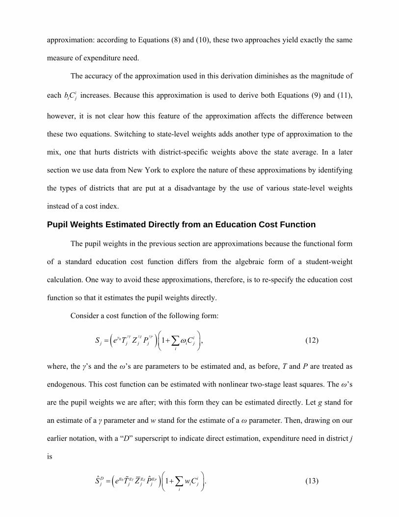
Pupil Weights Estimated Directly from an Education Cost Function
The pupil weights in the previous section are approximations because the functional form
of a standard education cost function differs from the algebraic form of a student-weight
calculation. One way to avoid these approximations, therefore, is to re-specify the education cost
function so that it estimates the pupil weights directly.
Consider a cost function of the following form:
( )0 1 ,T Z P ij j j j i j
i
S e T Z P Cγ γ γγ ω⎛ ⎞= +⎜ ⎟
⎝ ⎠∑ (12)
where, the γ’s and the ω’s are parameters to be estimated and, as before, T and P are treated as
endogenous. This cost function can be estimated with nonlinear two-stage least squares. The ω’s
are the pupil weights we are after; with this form they can be estimated directly. Let g stand for
an estimate of a γ parameter and w stand for the estimate of a ω parameter. Then, drawing on our
earlier notation, with a “D” superscript to indicate direct estimation, expenditure need in district j
is
( )0ˆ ˆ 1 .T Z Pg g g gD ij j j j i j
i
S e T Z P w C⎛ ⎞= +⎜ ⎟⎝ ⎠
∑ (13)

Recall the approximation noted earlier, namely, that exp{a} ≈ (1+a) when a is small.
With a = ii j
iCω∑ , this approximation translates Equation (12) into Equation (1), or vice versa.
Despite this algebraic connection between the two equations, however, they are substantially
different in practice. Compared to Equation (1), the nonlinear Equation (12) requires a more
complicated estimating procedure but results in a dramatic simplification in the calculation of
weights and student needs.
The obvious question to ask at this point is whether Equation (1) or (12) is a better
specification of the cost function, that is, which one provides a better explanation for variation in
school costs.8 This is, of course, an empirical question, which we address in a later section.
However, a specification test alone cannot determine which approach is best for policy purposes.
If the two approaches lead to similar results, then one must weigh the benefits of a relatively
simple estimating equation (Equation (1)) against the benefits of a relatively simple pupil-weight
calculation (Equation (12)). We return to this issue in our conclusion.
Pupil Weights in State Aid Formulas
The most common type of state aid formula is a foundation formula, which is used to
some degree in 43 states (Huang 2004). This type of formula is designed to bring all districts up
to a minimum spending level. Another type of aid formula is a so-called “guaranteed tax base”
plan, which is the main aid formula in three states and which is combined with a foundation plan
in ten others. Except in the case of Missouri, which relies exclusively on a GTB formula, the
weights in Table 1 refer to foundation plans.9 Following the emphasis in existing state aid
programs, we focus exclusively on the role of pupil weights in a foundation formula.10
A foundation formula sets aid per pupil at the difference between an expenditure target,
S , and the amount of money a district can raise at a standard tax rate, a rate set by state policy
makers. This amount of money is the tax rate, t , multiplied by the district’s tax base, Vj. To be
specific,

.j jA S tV= − (14)
A more general approach is to select an educational performance target and then to base the
formula on the expenditure needed to reach this target. Suppose S is the expenditure needed to
reach the desired level of student performance in a district with average costs, namely *ˆ
jS , as
defined by Equation (2). Then, as shown by Ladd and Yinger (1994), a cost index, Ij, can be
added to yield a performance-based foundation aid program:
*ˆ ˆ .j j j j j jA S I tV S tV= − = − (15)
With this approach, total aid to a district obviously equals aid per pupil multiplied by number of
pupils.
Pupil weights are designed to replace some, but not all, of the cost index. Specifically,
pupil weights do not account for differences in teacher costs or in enrollment effects across
districts. (A few states, namely, Colorado, Florida, Maryland, Massachusetts, and Texas,
combine pupil weights with an adjustment for teacher costs or the cost of living.)11 To bring in
pupil weights, therefore, one needs to use a spending base that reflects teacher wages but not
student characteristics, namely, 0ˆjS as defined by Equation (5). 12 Moreover, the number of
weighted pupils is
(1 ) .W i i i ij j j j j j
i iN N W N C N W C= + = +∑ ∑ (16)
Pupil weighting applies only to the expenditure target in a foundation aid formula, not to
the expected local contribution. Introducing pupil weights therefore leads to the following
formula for aid per (unweighted) pupil:
0ˆ .Wj
j j jj
NA S tV
N= − (17)

In this formula, the ratio of weighted to unweighted pupils plays the role of the student-need
component of an education cost index. The wage component of 0ˆjS multiplied by this ratio is
equivalent to a full cost index.
3. Results for New York State
To examine the implications of different approaches to estimating the cost of
disadvantaged students, we now use data from New York State for the 2000-2001 school year to
compare the distribution of state aid using Equation (15) with the aid using Equation (17) and
various forms of pupil weights. As shown in Table 3, we have data for 678 school districts and
have classified these districts into eight categories ranging from New York City to small rural
districts upstate.13 These districts differ substantially in terms of enrollment, wages, and the share
of students with various disadvantages. This table shows, for example, that the share of students
who applied for a free or reduced-price lunch, a commonly used measure of poverty, ranges from
74.9 percent in New York City to 11.2 percent in downstate suburbs. In addition, districts vary
widely in their child poverty rates and in their concentrations of students with limited English
proficiency or in special education. The special education variable, which provides one way to
measure the share of students with disabilities, is discussed in more detail below.
The last column of Table 3 presents a student performance index, which we will use in
our cost estimation. This index combines the passing rates on elementary and secondary math
and reading tests. The elementary tests cover both fourth and eighth grades, and the secondary
exams, called Regents exams, are given twice as much weight because students must pass them
to graduate from high school.14 The resulting index can range from 0 (no students pass any test)
to 200 (all students pass every test).
Cost Indexes

We begin by estimating standard education cost models. These models use the functional
form given in Equation (1), with operating spending per pupil as the dependent variable.
Following Duncombe, Lukemeyer, and Yinger (2003), the regressions also control for school-
district efficiency by including variables that have a conceptual link to efficiency, namely,
property value, income, and state aid—all on a per-pupil basis.
We estimate four versions of this model. These models are distinguished by (a) the
variable used to measure economic disadvantage and (b) whether special education students are
included. We use two different variables to measure economic disadvantage: the child poverty
rate in the school district, which is provided by the Census every two years, and the number of
students in grades K through 6 who sign up for a free lunch or for a reduced-price lunch.15 The
latter variable fluctuates significantly from year to year, so we use a two-year average in all of
our estimations.
Although these two variables are correlated, they are by no means identical.16 As shown
in Table 3, for example, the subsidized lunch variable tends to have a substantially larger value
than the child poverty variable. Moreover, the two variables have different strengths and
weaknesses. The Census poverty variable has the desirable feature that it cannot be manipulated
by school officials, but it is not available every year, it is often excluded from data bases
maintained by state education departments, and we have no evidence about its accuracy in years
not covered by a decennial census. The subsidized lunch variable has the advantages that it is
available every year, is included in many state data bases, and covers a broader population than
does the poverty variable. This variable has the disadvantage, however, that it reflects parental
participation decisions, and perhaps even school management policies. Given these contrasting
strengths and weaknesses, we do not believe that either variable dominates the other and we
present results using both of them.

One final difference between the two variables arises when another measure of student
disadvantage, the share of students with limited English proficiency (LEP), is added to the cost
model. As shown below, this LEP variable is highly significant in cost models that include the
census poverty variable. In contrast, this variable is not close to significant in models that include
the subsidized lunch variable. Thus, in case of New York, the subsidized lunch variable appears
to capture the cost effects both of poverty and of LEP, and the LEP variable is dropped from the
models in which the subsidized lunch variable appears.
The second distinction is whether the model includes a third measure of student
disadvantage, namely, the share of students in a special education program. We focus on a
measure of students with relatively severe disabilities, because these students have a relatively
large impact on educational costs and because the identification of these students is largely
insulated from district discretion. To be specific, this variable indicates the share of students who
require placement for 60 percent or more of the school day in a special class, or who require
special services or programs for 60 percent or more of the school day, or who require home or
hospital instruction for a period of more than 60 days. As we will see, this variable is highly
significant when it is included in a cost regression. However, this variable does not provide a full
analysis of the extra costs imposed by student disabilities. It does not include students with
relatively minor disabilities, for example, and it does not recognize the wide variations in
spending required for different students in the special education category. Moreover, some states
prefer to treat special education with categorical grants, instead of incorporating them into basic
measures of expenditure need and operating aid. As a result, we present all of our results with
and without special education students in the analysis.
These cost models include several cost variables in addition to student characteristics,
namely, teacher salaries (treated as endogenous) 17 and student enrollment categories. The
omitted enrollment category is districts with enrollment below 1,000 students. As explained

earlier, we do not include enrollment effects in our analyses of education costs, expenditure need,
or state aid.
Selected parameter estimates from the cost models are presented in Table 4. (Full results
for two of these cost models are presented in an appendix.18) The performance index is highly
significant in all cases, and the teacher wage variable has an elasticity close to unity. The student
characteristics also have large, statistically significant impacts on costs. A school district’s costs
increase with the share of students in poverty (whether measured by census poverty or subsidized
lunches), with limited English proficiency, or with a severe handicap. As noted earlier, the LEP
variable is not close to significant in models that use the subsidized lunch variable so it has been
dropped from these models.
The second panel of Table 4 presents results for Equation (12), which provides direct
estimates of the pupil weights. This equation also performs well, and the results in this panel are
similar to those in the first panel. We conducted specification tests to determine whether
Equation (1) (the first two panels) or Equation (12) (the last panel) provides a better fit for any
given column.19 We find that neither one of these models can be rejected in favor of the other;
that is, there is no statistical basis for selecting one of them. This choice must be made on other
grounds.
We then use the cost models in Table 4 to calculate cost indexes, using the approach
presented earlier. Our cost indexes reflect teacher wage costs (based on exogenous factors only)
and student characteristics. Not surprisingly, the resulting cost indexes vary widely by district
category. The first panel of Table 5 presents cost indexes based on the census poverty and LEP
variables. As shown in Table 5, our first cost index ranges from about 94 in upstate suburbs and
rural districts to 170.2 in New York City. This index also has relatively high values in Yonkers,
the Big Three, and downstate small cities, and intermediate values in downstate suburbs and
upstate small cities. The other cost indexes in the first panel exhibit similar patterns, with slightly
more variation across types of district when the special education variable is included.
The second panel of Table 5 presents cost indexes based on the share of students in
grades K through 6 who applied for a free or reduced-price lunch. The cost indexes in this panel
exhibit a larger variance than those in the first panel; the range in the first column, for example,
is from 84.4 in the upstate rural districts to 195.7 in New York City. Moreover, the index for
New York City exceeds 200 if special education students are included or if the pupil weights are
estimated directly.
Pupil Weights
Our next step is to calculate statewide pupil weights and to extract the pupil weights
estimated using Equation (12). The results are in Table 6. All the weights in this table are above
1.0, indicating that the cost of educating a student with any one of the three disadvantages we
observe is more than twice as high as the cost of educating a student with none of these
disadvantages. These weights are therefore higher than the weights used by any state except
Maryland (see Tables 1 and 2). Moreover, the weights for special education students are all
above 1.8.
In every case, the pupil weight goes up as one moves from column 1 to column 2 or from
column 2 to column 3. In other words, enrollment-weighted weights are larger than weights for
the average district, and directly estimated weights are larger than the weights calculated from a
standard education cost function. In addition, the poverty weights in the first and third models,
which are based on the census child poverty variable, decline by a small amount when students
requiring special education are added to the analysis, whereas the LEP weight increases slightly
when this change is made. Overall, this poverty weight ranges from 1.22 to 1.67, the LEP weight
ranges from 1.01 to 1.42, and the special education weight varies from 2.05 to 2.64.

Table 6 also presents estimated weights using the number of students applying for a
subsidized school lunch. Without either the special education variable or a direct estimating
procedure, the extra weight for an economically disadvantaged student is higher with the child
poverty variable than with the subsidized lunch variable. If the pupil weights are estimated
directly or if the special education variable is included in the estimation, the weight based on
subsidized lunch is larger, sometimes considerably larger, than the weight based on census
poverty.
Expenditure Need
Tables 7 and 8 compare expenditure need calculations using various approaches to the
cost of disadvantaged students. Table 7 is based on the census child poverty variable; Table 8
uses the subsidized lunch variable. The baseline in all cases is expenditure need with a full cost
index, which we regard as the most direct approach with the clearest conceptual foundation. Our
objective is to determine how much expenditure need diverges from this baseline when pupil
weights are used. As explained earlier, pupil weights approximate a cost index approach, so our
objective is equivalent to calculating which categories of districts are placed at a disadvantage by
this type of approximation. All our calculations include an adjustment for teacher wages.
The first row in each panel of Tables 7 and 8 compares aggregate expenditure need using
the weights identified in each column with aggregate expenditure need using a standard cost
index. A value below 1 indicates that aggregate expenditure need falls below the baseline value
and a value above 1 indicates that aggregate expenditure need is higher with those weights than
with the baseline cost index.
The first column in Table 7 shows how much expenditure need diverges from the
baseline when student characteristics are not accounted for at all. In the first panel, without
special education, this approach lowers aggregate expenditure need substantially, namely, by
almost 30 percent, compared to the baseline and places large cities at a significant disadvantage.

To be specific, the expenditure-need numbers for New York City, Yonkers, and the Big Three
fall about 40 percent below the baseline. In contrast, this approach leads to expenditure needs
that are only about 10 percent below the baseline in suburbs, both upstate and downstate.
The introduction of pupil weights brings the expenditure need calculations much closer
to the baseline for all types of districts. As shown in the second and third columns of the first
panel in Table 7, expenditure need falls no more then 8 percent below the baseline for big cities,
and no more than 1 percent below the baseline for suburbs (on average), when estimated
statewide pupil weights are used. Because the enrollment-weighted average weights tend to be
larger than the simple average weights, the use of an enrollment-weighted average boosts
expenditure need and narrows the divergence from the baseline. Indeed, the results in the third
column of Table 7 reveal almost no divergence from the baseline outside the large cities. The
divergence in the large cities is about 6 percent.
One simple approximation to estimated weights that is similar to the program passed in
Maryland is to use a weight of 1.0 for both poverty and LEP. The fourth column of the first panel
in Table 7 indicates that this approach provides a reasonable approximation to estimated weights
in the suburbs, where expenditure need is about 3 percent below the baseline, but only a rough
approximation in the big cities, where expenditure need falls about 15 percent below the baseline.
Finally, as shown in the last column of this panel, a calculation using weights that are directly
estimated comes very close to matching the results of a cost-index calculation. Indeed, with this
approach, New York City and the Big Three are only 1 percent below the baseline and no group
of districts falls above or below the baseline by as much as 3 percent. This result is not surprising;
as shown earlier, cost indexes and directly estimated pupil weights are approximately the same
thing.
The second panel of Table 7 provides comparable results based on a cost model with
special education students included. The results from this model are similar to those in the first
panel, although the first two models (with no weights and with simple average weights) and the
last model (with directly estimated weights) diverge from the baseline somewhat more than the
comparable models in the first panel. With enrollment-weighted weights, for example, the big
cities now fall about 10 percent below the baseline.
Table 8 presents results from an alternative pair of models that use the subsidized lunch
variable instead of the child poverty and LEP variables in both the baseline cost-index approach
and in all the calculations with pupil weights. This table reveals that leaving out weights
altogether results in an even larger divergence from the baseline with the subsidized lunch
variable than with the census poverty variable. Results in the other columns are similar to the
comparable ones in Table 7, particularly those based on directly estimated pupil weights. Recall
that with a single cost variable, as in the first panel of Table 8, a district-specific weight is
identical to a cost index. Hence, the only source of deviations from the baseline in the second
and third columns of this panel is the averaging procedure. The results in these two columns
therefore prove that moving from district-specific weights to statewide weights is unfair to high-
cost districts, particularly large cities, and that an enrollment-weighted average is preferable to a
simple average.
One contrast between Tables 7 and 8 can be found in the fourth column of the panel with
special education. In this case, the use of rounded weights (1.0 for subsidized lunch, 1.0 for LEP,
and 2.0 for special education) leads to a much larger underestimate of expenditure need,
particularly in the big cities, in Table 8 than in Table 7. This understatement is implicitly
predicted by the relevant directly estimated weights in Table 6, which are 2.1 for subsidized
lunch and 3.0 for special education.
Foundation Aid
As explained earlier, expenditure-need calculations feed into foundation aid formulas.
Thus, baseline state aid is the aid a district would receive with a foundation aid formula that

incorporates a full cost index. Our simulations define a baseline aid program by setting the
student performance index at 160, which is the current state average. Tables 9 and 10 show how
switching to pupil weights alters state aid for each category of district compared to this baseline.
To make the columns comparable, we hold the total budget constant (that is, equal to the baseline
amount) in all cases by raising or lowering the foundation level.20 Results for a baseline aid
program defined by a student performance index of 140 are very similar to those in Tables 9 and
10.
As in Tables 7 and 8, the first column of these two tables indicates the impact of ignoring
student characteristics. In Table 9, which examines aid programs based on the census poverty
and LEP variables, this step would cut the aid of the big-city districts by 20 percent or more
(compared to the baseline) and would greatly boost the aid of all other categories of districts.
Indeed, both the upstate and downstate suburbs would receive at least 46 percent more aid, on
average, with this approach than with the baseline approach.
The next four columns show that introducing pupil weights would bring all categories of
districts much closer to their baseline aid. Indeed, regardless of which pupil weights are used, the
big cities would all be within 8 percent of their baseline aid. In all cases, both the upstate and the
downstate suburbs receive more aid with pupil weights than with the baseline cost index. In
columns two through four, the aid in these districts is between 6 and 20 percent above the
baseline. Not surprisingly, the divergence from the baseline is smallest with directly estimated
weights (the last column). Indeed, in this case, aid to large cities and suburbs is always within 4.5
percent of the baseline amount.
Note that use of rounded weights is less disadvantageous to large cities in Table 9 than in
Table 7. This result reflects the fact that Table 9 holds the state aid budget constant and thereby,
in effect, eliminates the absolute decline in expenditure need in the earlier table. Finally, a
comparison of the two panels of Table 9 indicates that deviations from baseline aid are

somewhat larger when special education is included in the analysis. However, the difference
between a result in the second panel and the comparable result in the first panel is rarely above 2
percentage points.
As shown in Table 10, the patterns across districts are similar when the subsidized lunch
variable is used instead of the census poverty and LEP variables. In most cases, the divergence
from baseline is somewhat larger in Table 10 than for the comparable result in Table 9,
particularly when special education is included. With rounded weights and special education, for
example, the Big Three fall 8 percentage points below the baseline when child poverty is used
but 16 points below the baseline with subsidized lunch. Most of the other differences are
considerably smaller than this.
4. Conclusions and Policy Implications
There is widespread agreement among scholars, policy makers, and state courts that
school districts with relatively high concentrations of disadvantaged students should receive
relatively more state aid per pupil, all else equal. In the academic literature, the state-of-the-art
approach is to estimate an education cost function that includes measures of student disadvantage,
to calculate an education cost index on the basis of this estimation, and then to introduce this
education cost index into a foundation aid formula. Although a few state aid formulas contain
elements of the cost-index approach, most state aid formulas adjust for the presence of
disadvantaged students using pupil weights. Pupil weights appear to be more appealing to policy
makers than the more abstract notion of an education cost index. The key problem is that, in
almost every case, the weights that appear in state aid formulas are determined on an ad hoc
basis and are far below the weights estimated by scholars.
We show that a state aid formula using pupil weights can be thought of as an
approximation for a state aid formula using a cost index. The closeness of this approximation

cannot be determined a priori, but it can readily be calculated on the basis of an estimated
education cost function. We show that a state aid formula combining pupil weights and teacher
wage cost adjustments derived from a standard cost function distributes aid in a way that is
approximately the same as an aid formula based on a cost index. For the large, urban school
districts where most disadvantaged students are concentrated, aid based on statistically based
pupil weights provides a reasonable approximation for aid based on the preferred cost-index
approach. These two approaches differ somewhat more in their treatment of suburban and rural
school districts, which receive almost 20 percent more aid with some types of weights than with
a cost index. Finally, switching to a nonlinear cost function that estimates pupil weights directly
yields an aid formula that closely approximates the baseline approach in almost every case.
Indeed, with directly estimated weights, aid to big cities never falls more than 4 percent below
baseline aid (and aid to suburban districts falls within 5 percent of the baseline), unless special
education is included in the formula and subsidized lunch is the measure of poverty.
The pupil weights we estimate are much larger than the weights that appear in any state
aid formula except for Maryland’s. In a typical aid formula, the extra weight for a pupil from a
poor family or with limited English proficiency is about 25 percent. We estimate that these extra
weights should be between 111 and 215 percent. The use of pupil weights obviously results in a
much poorer approximation of our preferred aid formula when these lower weights are used. At
the extreme, defined by extra weights of zero, the aid received by large urban districts falls at
least 20 percent below the baseline level, and the aid received by suburban districts may exceed
the baseline by over 100 percent. The low weights used in most state aid programs yield results
not too different from this extreme case. The key problem, therefore, is not the use of pupil
weights per se; it is the use of pupil weights that are far below the levels supported by the
evidence.

We estimate similar weights for the census poverty and subsidized lunch variables. We
also conclude that in New York the LEP variable need not be included in an aid formula based
on the subsidized lunch variable, at least not when the weight on the subsidized lunch variable is
high enough, but we find that rounded weights of 1.0 for both subsidized lunch and LEP provide
a reasonable approximation to a cost-index approach. We also estimate an extra weight of at least
185 percent for a student in special education, but this weight obviously is linked to our special
education variable and may not apply to the special education variables that appear in state aid
formulas.
Overall, public officials who design state aid formulas face two key choices regarding
disadvantaged students.21 The first choice is whether to account for the extra cost of educating
these students using a cost index or pupil weights. Judging from the choices states have made so
far, the use of pupil weights appears to be a more appealing approach, and we show that, for
most districts, it can result in aid amounts that closely approximately the aid amounts from a
formula based on a cost index, which is the approach many scholars prefer.
The second choice is how to select pupil weights. The ad hoc process used in most states
is not up to the task. Indeed, the weights used by most states are far below the weights estimated
in this paper and by other scholars. These low weights result in aid payments that support far
lower levels of student performance in school districts with more disadvantaged students than in
other school districts. This outcome violates the key objective of a foundation aid formula,
namely, to bring all districts up to the same minimal performance standard. Finally, we find that
any pupil weights based on an estimated cost function provide a reasonable approximation to the
use of a full education cost index, but that an even better approximation can be obtained using
pupil weights estimated directly from a nonlinear cost function. We find no statistical basis for
preferring a standard cost function to this nonlinear version, so the choice of method depends on

whether policy makers prefer the complexity of the weight calculation with a standard cost
function to the complexity of a nonlinear estimating procedure.
A state aid program is not consistent with student performance objectives unless it
accounts for the higher cost of reaching a performance target in districts with a relatively large
share of disadvantaged students. The use of state aid formulas with extra weight for
disadvantaged students is a reasonable approach to this problem, but the fairness of this approach
can be greatly enhanced through the use of statistically based pupil weights.

Endnotes
1. The information in this table is based on legislative language in various published sources
and web sites, so it may not be complete or include all the latest aid revisions. We are
grateful to Yao Huang for compiling this information.
2. The figures in Table 2 predate the new aid program in Maryland; this new program may
be an exception to this claim.
3. Some scholars (e.g., Guthrie and Rothstein 1999) have criticized the cost-function
approach and have proposed alternatives, such as the use of professional educators to
identify the programs necessary to reach a given performance standard in a school with
many disadvantaged students. (The high pupil weights in Maryland are based on a study
that uses this so-called “professional judgment” approach. See Maryland Commission on
Education Finance, Equity and Excellence 2002.) In our judgment, however, a cost
function makes the best use of available information and is the preferred approach. For a
detailed discussion of the strengths and weaknesses of the various methods, see
Duncombe, Lukemeyer, and Yinger (2004).
4. A note on notation: A “^” indicates a spending level “required” to reach a performance
target under some specified set of conditions (or a wage level required to attract teachers),
a “~” indicates a policy parameter, and a “-“ indicates a mean value. In a few cases the
first and last symbols both appear, indicating the mean of a predicted value.
5. An alternative base in this type of calculation is the value of ˆjS in the average district.
This alternative base leads to similar results, but we find it less appealing because it shifts
the focus away from the average values of the student characteristics on which the
weights are based.
6. In spite of these problems, about one-third of the states give more aid to small or sparsely
settled districts. See Huang (2004).

7. If the data made it possible to identify students with multiple disadvantages (which ours
do not), then each combination of disadvantages could be treated as a separate cost
category.
8. The specifications in (1) and (12) are not the only possible ones. In fact, some scholars,
such as Gyimah-Brempong and Gyapong (1991), have used a more general specification.
9. Texas is one of the ten states with a first-tier foundation formula and a second-tier GTP
formula. It uses pupil weights in both tiers. See Huang (2004).
10. The widespread use of foundation plans reflects, among other things, a widespread
emphasis on an adequacy objective in recent state supreme court decisions concerning
education finance. See Lukemeyer (2002, 2004).
11. This information was provided by Yao Huang.
12. In principle, one could also include enrollment effects in this baseline spending number.
13. The major sources of data are various publications from the New York State Education
Department and New York State Office of the Comptroller. Child poverty rates and
population are from the 2000 Census of Population.
14. For more information on this index, see Duncombe, Lukemeyer and Yinger (2003). This
index is treated as endogenous. We used geographic proximity to identify instruments.
Specifically, our list of potential instruments consists of averages, minimum and
maximum values for adjacent school districts for various measures of fiscal capacity
(income, school aid, and property wealth), student need (poverty, LEP, subsidized lunch,
and special education), physical conditions (pupil density, population density,
enrollment), and student performance (test scores). To select instruments from this list,
we used three standard rules. The instruments must (1) make conceptual sense, (2) help to
explain the endogenous explanatory variables, and (3) not have a significant direct impact
on the dependent variable. We also implemented an over-identification test (Woolridge
2003) to check the exogeneity of our final set of instruments and the Bound, Jaeger, and
Baker (1995) procedure to check for weak instruments. The latter procedure is not
formally specified for a model like ours, so we examined various combinations of the
instruments and used the set that produced the highest F-test for most endogenous
variables. In most cases, the F-statistic was 5.0 or above, indicating reasonably strong
instruments for that endogenous variable. When estimating equation (12) we use the
same instruments selected for estimating (1).
15. The free lunch and reduced-price lunch programs are separate, but we combine them in
all our analyses. Eligibility rules and funding for these lunch programs is provided by the
federal government. Subsidized lunches are also offered after sixth grade but many
eligible students do not sign up for them, so a subsidized lunch variable for non-
elementary grades does not appear to be useful.
16. For the year 2000, for example, the correlation between the share of K-6 students who
sign up for a subsidized lunch and the child poverty rate is 0.773. Correlations in other
years are similar.
17. The teacher wage variable was first limited to teachers with five years or less of
experience. Teacher wages for individual teachers were then regressed on teacher
experience and whether the teacher had a graduate degree. The results of this regression
were used to construct a predicted teacher salary for each district for a teacher with
statewide average experience (among those with no more than 5 years of experience) and
average probability of a graduate degree. The potential instruments for this variable are
pupil density in the district, private wages in professional occupations, unemployment
rate, concentration of area teachers in the district, and the average (maximum and
minimum) salaries of adjacent districts. The final list was selected using the rules
presented in an earlier footnote.
18. The two regressions in this appendix table, along with comparable regressions for other
models, which are not presented, indicate that the performance index always has the
expected positive impact on costs and is statistically significant. The three efficiency
variables also have the expected signs and are significant in most cases, and all districts

in all enrollment classes except the largest have significantly lower costs per pupil than
districts in the smallest enrollment class.
19. We use the specification tests in Davidson and MacKinnon (2004, Chapter 15).
20. These simulations set the required local property tax rate, t , at 1.5 percent, which is
lower than the rate in most districts. Alternative tables that hold the foundation level
constant and allow the state aid budget to change are available from the authors upon
request, as are tables with a performance standard of 140 instead of 160.
21. Another key choice, which is not examined in this paper, is whether to use a teacher wage
index. Even with accurate pupil weights, an aid formula would not be fair to high-wage
locations unless in it included a wage index or a cost of living index. Only about a dozen
states have this type of index now (Huang 2004).

Table 1. Legislated Pupil Weights in Selected State Aid Programs
Pupil Weight For State Poverty LEP Handicap a Alaska yes Arizona 0.06 yes Colorado 0.115-0.3 Connecticut 0.25 b 0.1 Delaware yes c Florida 0.201 yes Georgia yes Idaho b c yes c Iowa 0.19 yes Kansas 0.1 0.2 Kentucky 0.15 b Louisiana 0.17 Massachusetts 0.343-0.464 b yes Maryland 1.0 1.2 Minnesota 0.01-0.6 b Mississippi 0.05 Missouri 0.22 New Hampshire 0.5-1.0 New Mexico 0.0915 yes Oklahoma 0.25 yes Oregon 0.25 0.5 yes South Carolina yes Texas 0.2 b 0.1 yes West Virginia yes Source: Compiled by Yao Huang based on NCES (2001); updated with information from various sources as cited in Huang (2004). a. Weights for students with handicaps vary widely depending on the nature of the handicap. b. These states also provide categorical grants for students in this category. c. These states adjust aid per teacher unit for weighted pupils, which is similar
to standard pupil weights.
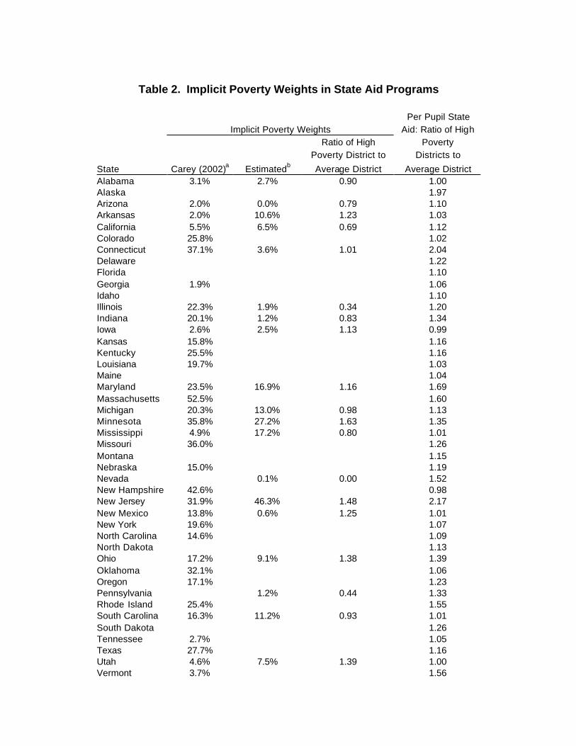
Table 2. Implicit Poverty Weights in State Aid Programs
Per Pupil State Implicit Poverty Weights Aid: Ratio of High Ratio of High Poverty Poverty District to Districts to
State Carey (2002)a Estimatedb Average District Average District Alabama 3.1% 2.7% 0.90 1.00 Alaska 1.97 Arizona 2.0% 0.0% 0.79 1.10 Arkansas 2.0% 10.6% 1.23 1.03 California 5.5% 6.5% 0.69 1.12 Colorado 25.8% 1.02 Connecticut 37.1% 3.6% 1.01 2.04 Delaware 1.22 Florida 1.10 Georgia 1.9% 1.06 Idaho 1.10 Illinois 22.3% 1.9% 0.34 1.20 Indiana 20.1% 1.2% 0.83 1.34 Iowa 2.6% 2.5% 1.13 0.99 Kansas 15.8% 1.16 Kentucky 25.5% 1.16 Louisiana 19.7% 1.03 Maine 1.04 Maryland 23.5% 16.9% 1.16 1.69 Massachusetts 52.5% 1.60 Michigan 20.3% 13.0% 0.98 1.13 Minnesota 35.8% 27.2% 1.63 1.35 Mississippi 4.9% 17.2% 0.80 1.01 Missouri 36.0% 1.26 Montana 1.15 Nebraska 15.0% 1.19 Nevada 0.1% 0.00 1.52 New Hampshire 42.6% 0.98 New Jersey 31.9% 46.3% 1.48 2.17 New Mexico 13.8% 0.6% 1.25 1.01 New York 19.6% 1.07 North Carolina 14.6% 1.09 North Dakota 1.13 Ohio 17.2% 9.1% 1.38 1.39 Oklahoma 32.1% 1.06 Oregon 17.1% 1.23 Pennsylvania 1.2% 0.44 1.33 Rhode Island 25.4% 1.55 South Carolina 16.3% 11.2% 0.93 1.01 South Dakota 1.26 Tennessee 2.7% 1.05 Texas 27.7% 1.16 Utah 4.6% 7.5% 1.39 1.00 Vermont 3.7% 1.56

Virginia 15.1% 12.1% 0.99 1.27 Washington 7.7% 12.6% 0.77 1.12 West Virginia 1.04 Wisconsin 10.0% 1.30 Wyoming 3.0% 1.55 a Source, Carey (2002). b Compensatory aid per child (5 to 17 years old) in poverty divided by total spending per pupil.

Table 3. Description of New York School Districts, 2001
Number of Average Teacher
Average Teacher Percent Child
Percent Subsidized Percent Special
Student Performance
Districts Enrollment Salary Poverty Lunch (K6) LEP1 Education2 Index3 Large Cities New York City
1 1,069,141 $39,561 34.90% 74.86% 12.32% 7.41% 103 Yonkers
1 24,847 $47,237 31.31% 59.72% 16.42% 8.52% 107 Upstate Big Three
3 35,575 $33,113 46.46% 74.53% 6.76% 9.46% 96 Small Cities
Downstate 7
5,647
$47,947
16.62%
33.48%
7.73%
6.07%
148
Upstate 49 4,324 $34,848 25.39% 41.73% 2.23% 6.68% 145 Suburbs
Downstate 168 3,387 $46,082 8.80% 11.22% 3.20% 4.85% 169
Upstate 242 2,450 $35,004 13.24% 19.39% 0.32% 4.44% 160
Rural
Upstate 207 1,113 $33,135 21.57% 29.09% 0.22% 4.33% 156 Statewide 678 1,657 $35,413 14.67% 21.81% 0.00% 4.72% 161 Note: Except in column 1, statewide figures are for the median district. 1LEP stand for “limited English proficiency.” 2The share of students who require placement for 60 percent or more of the school day in a special class, or require special services or programs for 60 percent or more of the school day, or require home or hospital instruction for a period of more than 60 days. 3Index reflects passing rates on elementary middle school and high school tests; maximum possible value is 200.

Table 4. Estimated Performance and Cost Coefficients
Without Special Ed. With Special Ed.
Census Poverty
Subsidized Lunch
Census Poverty
Subsidized Lunch
Standard Cost Models1 Performance index 0.0073 0.0105 0.0079 0.0140 (2.87) (3.12) (3.26) (3.2) Average teacher salary2 1.0006 1.4030 0.9392 1.3541 (8.06) (15.07) (8.82) (13.87) Percent child poverty (2000)3 1.3071 1.1424 (4.06) (4.17) 2-year avg. LEP3 0.9883 0.9908 (2.09) (2.46) K6 subsidized lunch rate3 0.9819 1.1258 (3.78) (3.68) Special education students3,4 1.9547 1.7762 (3.34) (2.63)
Direct Estimate of Pupil Weights5 Performance index 0.0075 0.0117 0.0079 0.0142 (2.85) (3.00) (3.32) (3.07) Average teacher salary2 1.0045 1.5639 0.9520 1.5519 (7.93) (9.69) (9.13) (8.11) Percent child poverty (2000)3 1.6672 1.5915 (3.21) (3.11) 2-year avg. LEP3 1.3078 1.4236 (1.81) (2.07) K6 subsidized lunch rate3 1.6896 2.1452 (2.36) (1.96) Special education students3,4 2.6440 3.0157 (2.69) (1.75) 1Estimated with linear two-stage least squares regression, with the student performance and teacher salaries treated as endogenous. Operating spending per pupil is the dependent variable; t-statistics are in parentheses. Full results for the first two columns of Panel 1 are in the appendix. 2For fulltime teachers with 1 to 5 years of experience. Expressed as a natural logarithm. 3Variables expressed as percentages. Coefficients are similar to elasticities. 4The share of students who require placement for 60 percent or more of the school day in a special class, or require special services or programs for 60 percent or more of the school day, or require home or hospital instruction for a period of more than 60 days. 5Estimated with nonlinear two-stage least squares regression. Other features are the same as in note 1.

Table 5. Cost Index Results1
Standard Cost Function Direct Weight Estimation Without
Special Ed. With
Special Ed. Without
Special Ed. With
Special Ed.
Using Census Poverty and LEP Large Cities New York City 170.2 172.0 165.4 169.9 Yonkers 159.2 166.3 155.9 164.3 Upstate Big Three 135.5 143.6 131.0 141.8 Small Cities Downstate 140.3 141.7 141.1 140.0 Upstate 110.8 113.9 110.6 112.6 Suburbs Downstate 114.8 115.1 114.7 113.7 Upstate 93.8 93.9 93.7 92.7 Rural Upstate 93.6 93.0 93.8 91.8 Using Percent of Students Receiving Subsidized Lunch Large Cities New York City 195.7 233.9 207.6 222.3 Yonkers 157.5 199.1 176.1 194.9 Upstate Big Three 142.8 181.7 148.4 160.0 Small Cities Downstate 146.0 165.8 165.1 173.5 Upstate 108.7 130.3 121.1 128.4 Suburbs Downstate 108.8 111.9 111.9 111.8 Upstate 86.7 93.2 94.0 93.7 Rural Upstate 84.4 96.0 94.8 96.0 1These indexes incorporate cost adjustments for teacher salaries and student needs, but not for enrollment. A district with state-wide average characteristics has an index value of 100.

Table 6. Estimated Pupil Weights
Enrollment- Weighted
Simple Average Average Directly Estimated
Using Census Poverty and LEP Without Special Education
Child Poverty 1.415 1.491 1.667
Limited English 1.007 1.030 1.308
Proficiency
With Special Education
Child Poverty 1.224 1.281 1.592
Limited English 1.009 1.033 1.424
Proficiency
Special Education 2.049 2.081 2.644
Using Share of Students Signed up for Subsidized Lunch Without Special Education
K6 Free and Reduced 1.108 1.294 1.690
Price Lunch Share
(2-year average) With Special Education
K6 Free and Reduced 1.361 1.552 2.145
Price Lunch Share
(2-year average)
Special Education 1.853 1.880 3.016

Table 7. Estimated Expenditure Need with Pupil Weights Relative to Baseline, Using
Census Child Poverty Variable
Regions
No Student Needs
Adjustment
Pupil Weights (Simple Avg.)
Pupil Weights (Enrollment -
Weighted Avg.)
Poverty and LEP Weights =1
Special Education Weight =21
Directly Estimated
Pupil Weights
Without Special Education Ratio of Total Cost With This Adjustment to Spending with Full Cost Index 0.713 0.956 0.967 0.898 1.004 Large Cities New York City 0.592 0.923 0.939 0.847 0.991 Yonkers 0.611 0.931 0.945 0.866 1.000 Upstate Big Three 0.583 0.921 0.938 0.833 0.986 Small Cities Downstate 0.764 0.980 0.990 0.937 1.027 Upstate 0.734 0.973 0.985 0.909 1.018 Suburbs Downstate 0.880 0.995 1.000 0.970 1.019 Upstate 0.899 1.001 1.006 0.972 1.019 Rural Upstate 0.814 0.992 1.002 0.941 1.024
With Special Education Ratio of Total Cost With This Adjustment to Spending with Full Cost Index 0.650 0.930 0.940 0.900 1.019 Large Cities New York City 0.539 0.890 0.903 0.851 1.003 Yonkers 0.539 0.889 0.901 0.856 1.003 Upstate Big Three 0.514 0.876 0.889 0.832 0.988 Small Cities Downstate 0.687 0.955 0.963 0.931 1.041 Upstate 0.662 0.945 0.955 0.912 1.031 Suburbs Downstate 0.796 0.980 0.985 0.966 1.038 Upstate 0.830 0.991 0.996 0.975 1.039 Rural Upstate 0.761 0.979 0.986 0.951 1.044 1Special education weight of 2 only applies in the model with special education students (lower panel).

Table 8. Estimated Expenditure Need with Pupil Weights Relative to Baseline, Using Subsidized Lunch Variable
No Student Needs
Adjustment
Pupil Weights (Simple Avg.)
Pupil Weights (Enrollment -
Weighted Avg.)
Poverty and LEP Weights
=1 Special
Education Weight =21
Directly Estimated
Pupil Weights
Without Special Education Ratio of Total Need With This Adjustment to Total Need with Full Cost Index 0.580 0.922 0.962 0.914 1.079 Large Cities New York City 0.453 0.875 0.926 0.874 1.070 Yonkers 0.509 0.914 0.962 0.942 1.100 Upstate Big Three 0.437 0.862 0.913 0.835 0.058 Small Cities Downstate 0.635 0.966 1.006 0.977 1.119 Upstate 0.588 0.947 0.990 0.916 1.113 Suburbs Downstate 0.813 0.986 1.007 0.992 1.066 Upstate 0.804 1.004 1.028 0.981 1.096 Rural Upstate 0.687 0.985 1.020 0.947 1.124 With Special Education Ratio of Total Need With This Adjustment to Total Need with Full Cost Index 0.470 0.852 0.899 0.802 1.075 Large Cities New York City 0.353 0.790 0.845 0.734 1.044 Yonkers 0.396 0.830 0.883 0.801 1.083 Upstate Big Three 0.327 0.758 0.811 0.686 1.009 Small Cities Downstate 0.525 0.911 0.957 0.877 1.136 Upstate 0.476 0.882 0.931 0.810 1.118 Suburbs Downstate 0.699 0.951 0.978 0.935 1.100 Upstate 0.714 0.985 1.016 0.938 1.145 Rural Upstate 0.595 0.952 0.996 0.877 1.162 1Special education weight of 2 only applies in the model with special education students (lower panel).

Table 9. State Aid Relative to Baseline for a Given State Aid Budget Using Census Child Poverty Rate and LEP Rate
No Student Needs
Adjustment
Pupil Weights
(Simple Avg.)
Pupil Weights (Enrollment -
Weighted Avg.)
Poverty and LEP Weights =1
Special Education
Weight =21
Directly Estimated
Pupil Weights
Without Special Education
Large Cities New York City 0.780 0.957 0.963 0.928 0.983 Yonkers 0.800 0.965 0.969 0.952 0.994 Upstate Big Three 0.788 0.959 0.965 0.917 0.979 Small Cities Downstate 1.136 1.050 1.046 1.079 1.046 Upstate 1.049 1.028 1.028 1.021 1.019 Suburbs Downstate 1.579 1.096 1.079 1.190 1.035 Upstate 1.459 1.084 1.071 1.146 1.026 Rural Upstate 1.230 1.062 1.058 1.078 1.031 With Special Education Large Cities New York City 0.781 0.949 0.952 0.934 0.981 Yonkers 0.767 0.944 0.946 0.937 0.981 Upstate Big Three 0.761 0.937 0.940 0.916 0.966 Small Cities Downstate 1.099 1.052 1.048 1.065 1.045 Upstate 1.034 1.027 1.026 1.023 1.018 Suburbs Downstate 1.527 1.121 1.108 1.165 1.045 Upstate 1.490 1.120 1.109 1.151 1.037 Rural Upstate 1.280 1.089 1.083 1.096 1.040 Note: Performance standard is set at an index value of 160; required local tax rate is set at 1.5 percent. 1Special education weight of 2 only applies in the model with special education students (lower panel).

Table 10. State Aid Relative to Baseline for a Given State Aid Budget Using Share of Students Signed up for Subsidized Lunch
No Student Needs
Adjustment
Pupil
Weights (Simple Avg.)
Pupil Weights (Enrollment -
Weighted Avg.)
Poverty and LEP Weights =1
Special Education Weight =21
Directly Estimated Pupil
Weights
Without Special Education
Large Cities New York City 0.740 0.937 0.950 0.942 0.980 Yonkers 0.846 0.988 0.996 1.039 1.017 Upstate Big Three 0.727 0.925 0.938 0.896 0.969 Small Cities Downstate 1.186 1.078 1.072 1.109 1.058 Upstate 0.039 1.038 1.036 0.999 1.032 Suburbs Downstate 1.972 1.145 1.092 1.170 0.976 Upstate 1.699 1.153 1.113 1.121 1.014 Rural Upstate 1.312 1.106 1.090 1.050 1.052 With Special Education Large Cities New York City 0.707 0.918 0.935 0.905 0.965 Yonkers 0.803 0.972 0.985 1.007 1.009 Upstate Big Three 0.662 0.880 0.896 0.842 0.930 Small Cities Downstate 1.195 1.112 1.111 1.150 1.097 Upstate 1.032 1.053 1.056 1.022 1.053 Suburbs Downstate 2.067 1.225 1.174 1.326 1.055 Upstate 1.927 1.281 1.237 1.306 1.112 Rural Upstate 1.430 1.190 1.178 1.155 1.124 Note: Performance standard is set at an index value of 160; required local tax rate is set at 1.5 percent. 1Special education weight of 2 only applies in the model with special education students (lower panel).

Table A1. Results of Education Cost Models1
With Census Poverty With Subsidized Lunch Variables Coefficient t-statistic Coefficient t-statistic Constant -2.6253 -2.53 -7.4910 -5.47 Performance index 0.0073 2.87 0.0105 3.12 Efficiency variables:2 Full value 0.0000 9.31 0.0000 10.30 Aid 0.8583 3.05 0.6872 2.39 Income 0.0000 1.55 0.0000 -0.70 Average teacher salary3 1.0006 8.06 1.4030 15.07 Percent child poverty (2000)4 1.3071 4.06 2-year avg. LEP4 0.9883 2.09 K6 subsidized lunch rate4 0.9819 3.78 Enrollment classes:5 1,000-2,000 students -0.0823 -3.31 -0.0859 -3.28 2,000-3,000 students -0.0896 -3.00 -0.0957 -3.15 3,000-5,000 students -0.1067 -2.87 -0.1218 -3.35 5,000-7,000 students -0.0915 -2.27 -0.1110 -2.73 7,000-15,000 students -0.1019 -2.12 -0.1208 -2.53 Over 15,000 students 0.0236 0.22 0.0308 0.27 Adjusted R-square 0.485 0.457 1Estimated with linear two-stage least squares regression, with student performance and teacher salaries treated as endogenous; operating spending per pupil is the dependent variable. 2Calculated as the difference between district value and the average in peer group. 3 For fulltime teachers with 1 to 5 years of experience. Expressed as a natural logarithm. 4All variables expressed as a percentage. Coefficients are similar to elasticities. 5The base enrollment is 0 to 1000 students. The coefficients can be interpreted as the percent change in costs from being in this enrollment class compared to the base enrollment class.

References
Abbott v. Burke, 119 N.J. 287, 575 A.2d 359 (New Jersey) 1990 (Abbott II). Andrews, M., W.D. Duncombe, and J. Yinger. 2002. “Revisiting Economies of Size in
Education: Are We Any Closer to a Consensus?” Economics of Education Review 21(3) (June): 245-262.
Bound, J., D.A. Jaeger, and R. Baker. 1995. “Problems with Instrumental Variables Estimation
When the Correlation between the Instruments and the Endogenous Explanatory Variables is Weak.” Journal of the American Statistical Association 90 (June): 443-450.
Bradbury, K.L., H.F. Ladd, M. Perrault, A. Reschovsky and J. Yinger. 1984. “State Aid to Offset
Fiscal Disparities Across Communities.” National Tax Journal 37(June): 151-170. Bradford, D., R.A. Malt, W.E. Oates. 1969. “The Rising Cost of Local Public Services: Some
Evidence and Reflections.” The National Tax Journal 22(2): 185-202. Campaign for Fiscal Equity (CFE), v. The State of New York. June 26, 2003. (Not yet filed) Carey, K. 2002. “State Poverty Based Education Funding: A Survey of Current Programs and
Options for Improvement.” Washington, DC: Center on Budget and Policy Priorities. Courant, P.N., E. Gramlich, and S. Loeb. 1995. “A Report on School Finance and Educational
Reform in Michigan.” In T.A. Downes and W.A. Tests (eds.), Midwest Approaches to School Reform. Chicago: Federal Reserve Bank of Chicago, pp.5-33.
Davidson, R., and J.G. MacKinnon. 2004. Econometric Theory and Methods. New York: Oxford
University Press. Downes, T.A., and T.F. Pogue. 1994. “Adjusting School Aid Formulas for the Higher Cost of
Educating Disadvantaged Students.” National Tax Journal 67(March): 89-110. Duncombe, W. D. 2002. “Estimating the Cost of an Adequate Education in New York.” CPR
Working Paper No. 44. Syracuse, NY: Center for Policy Research. Duncombe, W. D., and J.M. Johnston. 2004. “The Impacts of School Finance Reform in Kansas:
Equity Is in the Eye of the Beholder.” In J. Yinger (ed.), Helping Children Left Behind: State Aid and the Pursuit of Educational Equity. Cambridge, MA: MIT Press, pp. 147-193.
Duncombe, W. D., A. Lukemeyer and J. Yinger. 2003. “Financing an Adequate Education: A
Case Study of New York.” In W.J. Fowler, Jr. (ed.) Developments in School Finance: 2001-2002. Washington, DC: U.S. Department of Education, National Center for Education Statistics, June. Available at http://www-cpr.maxwell.syr.edu/efap/ 07.Duncombe_18June.pdf. (Last accessed 3/4/2004.)

Duncombe, W. D., A. Lukemeyer and J. Yinger. 2004. “Education Finance Reform in New York:
Calculating the Cost of a ‘Sound Basic Education’ in New York City.” Center for Policy Research Policy Brief 28/2004, Syracuse University, Syracuse, NY. Available at http://cpr.maxwell.syr.edu/efap.
Duncombe, W. D., J. Ruggiero and J. Yinger. 1996. “Alternative Approaches to Measuring the
Cost of Education.” In H.F. Ladd (ed.), Holding Schools Accountable: Performance-Based Reform in Education. Washington, DC: The Brookings Institute, pp. 327-356.
Duncombe, W. D., and J. Yinger. 1997. “Why is it So Hard to Help Central City Schools?”
Journal of Policy Analysis and Management 16: 85-113. Duncombe, W. D., and J. Yinger. 1998. “School Finance Reform: Aid Formulas and Equity
Objectives.” National Tax Journal (June): 239-262. Duncombe, W. D., and J. Yinger. 2000. “Financing Higher Student Performance Standards: The
Case of New York State? “ Economics of Education Review 19 (October): 363-386. Guthrie, J.W., and R. Rothstein. 1999. “Enabling ‘Adequacy’ to Achieve Reality: Translating
Adequacy into State School Finance Distribution Arrangements.” In H.F. Ladd, R. Chalk and J. Hansen (eds.), Equity and Adequacy in Education Finance: Issues and Perspectives. Washington, DC: National Academy Press, pp. 209-259.
Gyimah-Brempong, K., and A.O. Gyapong. 1991. “Production of Education: Are Socioeconomic
Characteristics Important Factors?” Eastern Economic Journal 17 (October-December): 507-521.
Huang, Y. 2004. Appendix B: “A Guide to State Operating Aid Programs for Elementary and
Secondary Education.” In J. Yinger (ed.), Helping Children Left Behind: State Aid and the Pursuit of Educational Equity. Cambridge, MA: MIT Press, pp. 331-351.
Imazeki, J., and A. Reschovsky. 2004. “School Finance Reform in Texas: A Never Ending
Story.” In J. Yinger (ed.), Helping Children Left Behind: State Aid and the Pursuit of Educational Equity. Cambridge, MA: MIT Press, pp. 251-281.
Ladd, H.F., and J. Yinger. 1994. “The Case of Equalizing Aid.” National Tax Journal 47(1):
211-224. Lukemeyer, A. 2004. “Financing a Constitutional Education: Views from the Bench.” In J.
Yinger (ed.), Helping Children Left Behind: State Aid and the Pursuit of Educational Equity. Cambridge, MA: MIT Press, pp. 59-85.
Lukemeyer, A. 2002. “Courts as Policymakers: School Finance Reform Litigation.” New York,
LFB Scholarly Publications. Maryland Commission on Education Finance, Equity, and Excellence. 2002. Final Report.
Baltimore: Maryland Commission on Education Finance, Equity, and Excellence. Available at http://mlis.state.md.us/other/education/. (Last accessed 6/14/04.)

Ratcliffe, K., B. Riddle, and J. Yinger. 1990. “The Fiscal Condition of School Districts in
Nebraska: Is Small Beautiful?” Economics of Education Review 9(January): 81-99. Reschovsky, A., and J. Imazeki. 1998. “The Development of School Finance Formulas to
Guarantee the Provision of Adequate Education to Low-Income Students.” In W.J. Fowler Jr. (ed.), Developments in School Finance, 1997: Does Money Matter? Washington, D.C.: U.S. Department of Education, National Center for Educational Statistics, pp. 121-148.
Reschovsky, A., and J. Imazeki. 2001. “Achieving Educational Adequacy Through School
Finance Reform.” Journal of Education Finance 26(4) (Spring): 373-396. Reschovsky, A., and J. Imazeki. 2003. “Let No Child Be Left Behind: Determining the Cost of
Improving Student Performance.” Public Finance Review 31 (May): 263-290. Woolridge, J. M. 2003. Introductory Econometrics: A Modern Approach. South-Western,
Independence, Mason, Ohio: Thomson Learning, 2nd Edition.