How many ENSO flavors can we distinguish?*

Nathaniel C. Johnson

International Pacific Research Center, SOEST, University of Hawaii at Manoa,

Honolulu, Hawaii

Journal of Climate

Revised December 23, 2012

____________________ *International Pacific Research Center publication number XXX

Corresponding author address: Nathaniel Johnson, IPRC, University of Hawaii at Manoa, 401 POST Building,

Honolulu, HI, 96822.

E-mail: natj@hawaii.edu

1

ABSTRACT 1

2

It is now widely recognized that the El Niño-Southern Oscillation (ENSO) occurs in 3

more than one form, with the canonical eastern Pacific (EP) and more recently recognized 4

central Pacific (CP) ENSO types receiving the most focus. Given that these various ENSO 5

“flavors” may contribute to climate variability and long-term trends in unique ways, and that 6

ENSO variability is not limited to these two types, this study presents a framework that treats 7

ENSO as a continuum but determines a finite, maximum number of statistically distinguishable 8

representative ENSO patterns. A neural network-based cluster analysis called self-organizing 9

map (SOM) analysis paired with a statistical distinguishability test determine nine unique 10

patterns that characterize the September – February tropical Pacific SST anomaly fields for the 11

period from 1950 through 2011. These nine patterns represent the flavors of ENSO, which 12

include EP, CP, and mixed ENSO patterns. Over the 1950-2011 period, the most significant 13

trends reflect changes in La Niña patterns, with a shift in dominance of La Niña-like patterns 14

with weak or negative west Pacific warm pool SST anomalies until the mid 1970s, followed by a 15

dominance of La Niña-like patterns with positive west Pacific warm pool SST anomalies, 16

particularly after the mid 1990s. Both an EP and especially a CP El Niño pattern experienced 17

positive frequency trends, but these trends are indistinguishable from natural variability. 18

Overall, changes in frequency within the ENSO continuum contributed to the pattern of tropical 19

Pacific warming, particularly in the equatorial eastern Pacific and especially in relation to 20

changes of the La Niña-like rather than El Niño-like patterns. 21

22

23

24

2

1. Introduction 25

The El Niño-Southern Oscillation (ENSO) is the dominant mode of tropical atmosphere-26

ocean interaction on interannual timescales, with impacts that span much of the globe 27

(Ropelewski and Halpert 1987; Trenberth and Caron 2000). Typically, ENSO episodes have 28

been identified through the monitoring of sea surface temperature (SST) anomalies in the 29

equatorial Pacific region, most notably the so-called Niño 3.4 region (5ᵒS - 5ᵒN, 120 - 170ᵒW). 30

However, recent studies have made it increasingly clear that traditional definitions of ENSO 31

episodes fail to distinguish two unique types of El Niño episode, the canonical El Niño that is 32

centered in the eastern equatorial Pacific and the more recently recognized El Niño that is 33

centered farther west near the International Date Line. This latter type, which has been referred 34

by various names such as the “dateline El Niño” (Larkin and Harrison 2005), “El Niño Modoki” 35

(Ashok et al. 2007), “warm pool El Niño” (Kug et al. 2009), and “central Pacific El Niño” (Yeh 36

et al. 2009), has received increased attention because of its unique underlying dynamics (Kao 37

and Yu 2009; Kug et al. 2009; Newman et al. 2011a,b; Yu and Kim 2011), global impacts 38

(Larkin and Harrison 2005; Weng et al. 2007; Ashok et al. 2007; Mo 2010; Hu et al. 2012), and 39

potential trends under global warming (Yeh et al. 2009) relative to those of the eastern Pacific 40

(EP) El Niño. On the basis of climate model simulations analyzed in the IPCC Fourth 41

Assessment Report, Yeh et al. (2009) suggest that the relative frequency of central Pacific (CP) 42

El Niño episodes may increase under anthropogenic global warming in response to changes in 43

the equatorial Pacific mean thermocline. However, the recent increasing trend in the frequency 44

of CP El Niño episodes (Lee and McPhaden 2010) may be indistinguishable from natural 45

variability (Newman et al. 2011b; Yeh et al. 2011). 46

3

The recent focus on the distinction between the EP and CP El Niño is consistent with the 47

notion that ENSO may come in many different “flavors” (Trenberth and Stepaniak 2001) that are 48

distinct from the canonical El Niño and La Niña composites and cannot be characterized by a 49

single index. In order to describe the structure and evolution of these various flavors, 50

investigators have increasingly considered multiple indices that capture the zonal gradient of 51

equatorial Pacific SST anomalies such as the “Trans-Niño Index” (Trenberth and Stepaniak 52

2001) or, more commonly for the identification of EP and CP El Niño episodes, a comparison 53

between Niño 3 (5ᵒS - 5ᵒN, 150ᵒ - 90ᵒW) and Niño 4 region (5ᵒS - 5ᵒN, 160ᵒE - 150ᵒW) SST 54

anomalies. Although this additional information clearly reveals some of the distinct properties 55

between various ENSO episodes, such subjective index choices are not necessarily optimal for 56

describing the various ENSO flavors that are discernible in the observational record. 57

Another common approach for distinguishing tropical SST patterns is through empirical 58

orthogonal function (EOF) analysis, but this method is not guaranteed to reveal physically 59

interpretable SST modes (e.g., L’Heureux et al. 2012). In particular, the leading EOF of tropical 60

Pacific SSTs generally resembles the canonical EP ENSO pattern, and either the second (e.g., 61

Ashok et al. 2007) or third (e.g., L’Heureux et al. 2012) EOF resembles the CP ENSO pattern. 62

However, this second or third EOF also tends to capture the spatial asymmetry between the EP 63

El Niño and La Niña patterns (Hoerling et al. 1997; Rodgers et al. 2004), which means that this 64

particular EOF is not uniquely identified with CP ENSO episodes. This complication highlights 65

one of the potential pitfalls of using a linear, orthogonal method like EOF analysis to 66

characterize nonlinear, non-orthogonal SST patterns. 67

In this study we consider a new perspective and methodology for describing ENSO 68

flavors. Under the perspective presented here, we recognize that there is a continuum of ENSO 69

4

states but that the relatively brief observational record limits the number of distinct ENSO 70

flavors that we can distinguish. Here we consider a methodology that treats ENSO as a 71

continuum but also determines a finite, maximum number of statistically distinguishable ENSO 72

flavors. This approach is based on a pairing of a type of neural network-based cluster analysis, 73

called self-organizing map (SOM) analysis, with a statistical distinguishability test, described 74

more thoroughly in the following section. This approach represents a more objective partitioning 75

of the equatorial Pacific SST data than the standard approach of partitioning by somewhat 76

subjective SST indices. In addition, this approach, which is constrained by neither linearity nor 77

orthogonality, avoids the disadvantages of common linear methods such as EOF analysis and 78

often results in more easily interpretable physical patterns (Reusch et al. 2005; Liu et al. 2006; 79

Johnson et al. 2008). 80

Because tropical SST trends play a critical role in remote, regional temperature and 81

precipitation trends (Shin and Sardeshmukh 2011) and tropical precipitation and circulation 82

changes (Xie et al. 2010; Johnson and Xie 2010; Ma et al. 2012; Tokinaga et al. 2012), it is 83

worthwhile to examine how changes in the frequency of different ENSO flavors impact the long-84

term SST trend. As demonstrated and discussed in the following three sections, the framework 85

adopted here allows us to connect the long-term SST trend to changes in the frequency 86

distribution of interannually varying SST patterns. 87

The remainder of the paper is organized as follows. Section 2 provides a description of 88

the general framework, methodology, and data used in this analysis. Section 3 presents the main 89

results, which include the SOM cluster patterns and the results of the trend analysis. The paper 90

concludes with discussion and conclusions in Sections 4 and 5. 91

92

5

2. Data and Methodology 93

In this section we examine the approach for determining the ENSO region SST clusters 94

and then determining the maximum number of distinguishable clusters. 95

96

a. Self-organizing map SST cluster patterns 97

98

Conceptually, we would expect that determining the maximum number of distinguishable 99

ENSO flavors would require a partitioning of tropical Pacific SST fields into groups that 100

maximize similarity within groups while also maximizing the dissimilarity between groups. 101

Computationally, this sort of partitioning may be accomplished either by K-means cluster or 102

SOM analysis. Specifically, K-means cluster analysis treats each SST field as an M-dimensional 103

vector, where M is the number of grid points, and minimizes the sum of squared distances 104

between each SST field and the nearest of the K cluster centroids. There are several reasonable 105

choices for a distance metric, but Euclidean distance is perhaps most commonly used, and is 106

used in the analysis presented here. The clusters are most commonly determined through an 107

iterative, two-step procedure described as such: Given an initial assignment of K cluster 108

centroids, which may be a random distribution, the first step is the assignment of the data vectors 109

(SST fields in this case) to the nearest cluster centroid, and the second step is the calculation of 110

the new cluster centroids. These two steps are repeated until the cluster assignments no longer 111

change, which corresponds to a local minimum of the sum of squared distances described above. 112

The value of K must be specified prior to the cluster analysis, and the method for determining K 113

for this problem is discussed in Section 2b. K-means cluster analysis has remained a popular 114

method of cluster analysis in the atmospheric and ocean sciences for decades (e.g., Michelangeli 115

6

et al. 1995; Christiansen 2007; Johnson and Feldstein 2010; Riddle et al. 2012; Freeman et al. 116

2012). 117

SOM analysis (Kohonen 2001) is a relatively new neural network-based cluster analysis 118

that bears strong similarities to K-means clustering and has increased in popularity in the 119

atmospheric and ocean sciences over the past decade (e.g., Hewitson and Crane 2002; 120

Richardson et al. 2003; Liu et al. 2006; Leloup et al. 2007; Johnson et al. 2008; Jin et al. 2010; 121

Lee et al. 2011; Chu et al. 2012). SOM analysis most significantly distinguishes itself from K-122

means cluster analysis through the addition of a topological ordering on a low-dimensional 123

(typically one- or two-dimensional) map. In other words, the clusters “self-organize” such that 124

similar clusters are located close together on this low-dimensional map, often displayed as a grid, 125

and dissimilar clusters are located farther apart. This combination of clustering and topological 126

ordering makes SOM analysis effective for providing a visualization of the continuum of 127

patterns within a dataset. Similar to the objectives of this study, SOM analysis has been used in 128

previous studies to describe the continuum of atmospheric teleconnection patterns (e.g., Johnson 129

et al. 2008; Lee et al. 2011) and to describe decadal changes in ENSO (Leloup et al. 2007). 130

The self-organizing nature of SOM analysis owes to a component called the 131

neighborhood function, with an associated parameter called the neighborhood radius. When the 132

neighborhood radius is greater than zero, the clusters become organized within the low-133

dimensional map. When the neighborhood radius is set to zero, the SOM algorithm reduces to 134

the K-means clustering algorithm. Thus, SOM analysis can be considered a “constrained version 135

of K-means clustering” (Hastie et al. 2009). In the present analysis, a one-dimensional SOM 136

analysis is performed such that the neighborhood radius gradually shrinks to a value of zero. 137

Therefore, the SOM patterns become topologically ordered along a line when the neighborhood 138

7

radius is greater than zero, but the algorithm used to determine the cluster patterns converges to 139

the K-means clustering algorithm. The SOM approach is chosen to ensure that similar ENSO 140

flavors are grouped together, but we would expect to see similar results with K-means cluster 141

analysis. See the appendix of Johnson et al. (2008) for a more thorough description of the basic 142

SOM methodology and Liu et al. (2006) for additional information on recommended SOM 143

parameter choices. 144

In this study, we consider ENSO flavors to be represented by SOM SST anomaly patterns 145

in the equatorial Pacific domain. We use September – February mean SST data for the period 146

from 1950 through 2011 derived from the Extended Reconstructed Sea Surface Temperature 147

Dataset, Version 3b (ERSST v3b; Xue et al. 2003; Smith et al. 2008). The September – 148

February period is used because of the seasonal phase locking of ENSO, which results in the vast 149

majority of ENSO episodes peaking during boreal fall or winter. The starting year of 1950 is 150

chosen because of the improved spatial and temporal coverage of SST data that begins around 151

that time (Deser et al. 2010; see their Fig. 3). In addition, prior to 1950 the SST patterns of 152

ENSO episodes may depend strongly on the method of reconstruction for the SST dataset (Giese 153

and Ray 2011; Ray and Giese 2012). The chosen domain covers the tropical Pacific region 154

between 120ᵒE and 50ᵒW and between 25ᵒS and 25ᵒN. The ERSST v3b data are on a 2ᵒ 155

latitude-longitude grid, but because the analysis described in the following section requires equal 156

weight to be placed on each grid point, the data are linearly interpolated to an equal-area grid 157

with 1ᵒ latitudinal spacing and longitudinal spacing that increases from 1ᵒ at the equator to 158

approximately 1.1ᵒ at 25ᵒ latitude. Anomalies are calculated by subtracting the seasonal cycle 159

for the 1981-2010 base period. The choice of the most recent 30-year climatology is based on 160

the standard practice of the National Oceanic and Atmospheric Administration (NOAA) Climate 161

8

Prediction Center (CPC), but the focus of this study, the spatial variations and trends of ENSO 162

flavors, is not sensitive to this choice of base period. SOM analysis is performed on the SST 163

anomaly data for various choices of K, as described in section 2b. Because the analysis 164

converges to a local rather than global minimum of the error function described at the beginning 165

of this section, the SOM analyses and all tests of Section 2b are repeated five times without any 166

noticeable change in results. Thus, the results presented here are robust. All SOM calculations 167

are performed with the Matlab SOM Toolbox (Vesanto et al. 2000) that is freely available on the 168

Web (http://www.cis.hut.fi/somtoolbox/). 169

170

b. Determining the maximum number of distinguishable ENSO flavors 171

172

Because K must be specified prior to a K-means cluster or SOM analysis, one challenge 173

in any cluster analysis is the determination of the optimal number of clusters. Many studies have 174

suggested various useful heuristic methods for determining K (e.g., Michelangeli et al. 1995; 175

Christiansen 2007; Hastie et al. 2009; Riddle et al. 2012), but an objective optimal K has 176

remained elusive. In this study we consider a new criterion for choosing K: the maximum 177

number such that all clusters are statistically distinguishable from another. Thus, if K* is the 178

optimal K by this criterion, then we can determine K* unique cluster patterns, but K*+1 clusters 179

would result in two or more clusters that are indistinguishable by this statistical definition. In the 180

present application, K* would refer to the maximum number of statistically discernible ENSO 181

flavors. 182

The determination of whether two cluster patterns are statistically distinguishable 183

requires a test of field significance. Often times in the atmospheric and ocean sciences, field 184

9

significance tests have been conducted through Monte Carlo resampling methods (Livezey and 185

Chen 1983). Recently, another field significance approach based on the “false discovery rate” 186

(FDR) has been introduced to the climate sciences (Benjamini and Hochberg 1995; Wilks 2006). 187

The FDR refers to the expected proportion of local null hypotheses that are rejected but are 188

actually true. In the present application, the local hypotheses being evaluated are whether the 189

SST anomalies at each grid point in cluster pattern i are significantly different from the 190

corresponding SST anomalies in cluster pattern j. If at least one local test has a p-value that 191

satisfies the specified FDR criterion, typically q = 0.05, then the cluster patterns are statistically 192

distinguishable also at the level q. If no local tests meet the FDR criterion, then the cluster 193

patterns are statistically indistinguishable. Further explanation of this test is provided below. 194

The FDR approach has a number of advantages over conventional field significance tests, 195

including generally better test power, robust results even when the local test results are correlated 196

with each other, and the identification of significant local tests while controlling the proportion 197

of false rejections (Wilks 2006). In addition, FDR tests are much more computationally efficient 198

than Monte Carlo methods, and so a large number of field significance tests can be conducted 199

with little computational effort, as required for the tests described here. 200

To determine if SOM cluster i is statistically distinguishable from SOM cluster j, we first 201

calculate the p-values (two-sided) at each grid point corresponding to the Student’s t distribution 202

for a difference of means, where the null hypothesis is that the local SST composite anomalies 203

are the same in both clusters. This test is based on the recognition that SOM cluster pattern i (j) 204

with ni (nj) cluster members is equivalent to an SST composite pattern with ni (nj) samples that 205

10

comprise the composite1. Each of the ni or nj cluster members is a seasonal SST anomaly field 206

assigned to that cluster on the basis of minimum Euclidean distance. For each pair of cluster 207

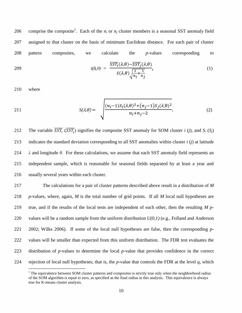
pattern composites, we calculate the p-values corresponding to 208

t(λ,θ) =

(1) 209

where 210

S(λ θ) =

(2) 211

The variable ( ) signifies the composite SST anomaly for SOM cluster i (j), and Si (Sj) 212

indicates the standard deviation corresponding to all SST anomalies within cluster i (j) at latitude 213

λ and longitude θ. For these calculations, we assume that each SST anomaly field represents an 214

independent sample, which is reasonable for seasonal fields separated by at least a year and 215

usually several years within each cluster. 216

The calculations for a pair of cluster patterns described above result in a distribution of M 217

p-values, where, again, M is the total number of grid points. If all M local null hypotheses are 218

true, and if the results of the local tests are independent of each other, then the resulting M p-219

values will be a random sample from the uniform distribution U(0,1) (e.g., Folland and Anderson 220

2002; Wilks 2006). If some of the local null hypotheses are false, then the corresponding p-221

values will be smaller than expected from this uniform distribution. The FDR test evaluates the 222

distribution of p-values to determine the local p-value that provides confidence in the correct 223

rejection of local null hypotheses; that is, the p-value that controls the FDR at the level q, which 224

1 The equivalence between SOM cluster patterns and composites is strictly true only when the neighborhood radius

of the SOM algorithm is equal to zero, as specified as the final radius in this analysis. This equivalence is always

true for K-means cluster analysis.

11

is also the global or field significance level αglobal. This test is conducted as follows. Let p(m) 225

denote the mth smallest of the M p-values. The FDR can be controlled at the level q for 226

. (3) 227

All local tests that yield a p-value less than or equal to the largest p-value that satisfies the right-228

hand side of (3) are deemed significant, which means that the expected fraction of local null 229

hypotheses that are actually true for those tests is less than or equal to q. If no local tests meet 230

the criterion specified in (3), then the patterns are statistically indistinguishable. In the present 231

application, we shall not focus on the specific value of pFDR, but instead shall focus on whether 232

or not any local tests satisfy (3) for q = 0.05; that is, whether or not the cluster patterns are 233

statistically distinguishable at the 95% confidence level. Although the assumption of 234

independent local tests does not hold in this case due to high spatial correlation in the SST fields, 235

the results of FDR tests do not appear sensitive to this independence assumption (Wilks 2006). 236

For K SOM cluster patterns there are K(K-1)/2 possible pairs of patterns to compare with 237

the test described above. To determine K*, we perform the SOM analysis for values of K that 238

increase from two to 20 at an increment of one, perform the K(K-1)/2 field significance tests, as 239

described above, for each choice of K, and count the number of SOM cluster pattern pairs that 240

are statistically indistinguishable. The maximum number of statistically distinguishable ENSO 241

flavors, K*, is the largest value of K with zero statistically indistinguishable cluster pattern pairs. 242

243

3. Results 244

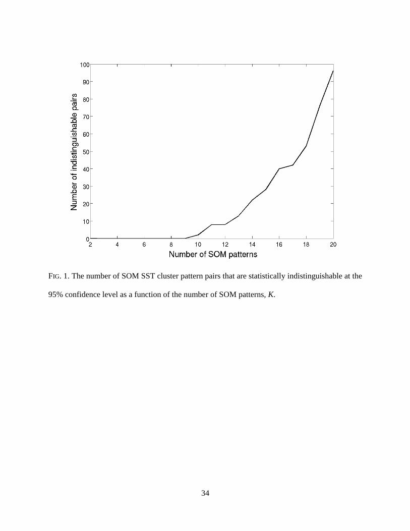
We first examine the results of the field significance tests described above. Figure 1 245

illustrates the number of statistically indistinguishable cluster pattern pairs as a function of K. 246

12

We see that as K is increased from two to nine, all pairs of cluster patterns for each K remain 247

statistically distinguishable. When K is increased to ten, however, the number of statistically 248

indistinguishable pairs rises above zero. As we would expect, the number of indistinguishable 249

pairs rises monotonically with K above nine2. Thus, by the reasoning stated above, the 250

maximum number of statistically distinguishable ENSO flavors is determined to be nine. 251

The value of K* may vary slightly based on the domain chosen to represent ENSO 252

flavors. Reasons for the slight variations include changes in the number of spatial degrees of 253

freedom, the convergence of cluster analyses to local rather than global minima of the error 254

functions, and the use of a sharp significance threshold of αglobal = 0.05. However, we do obtain 255

the same value of K* when we change the northern and southern boundaries to 20ᵒN/S or move 256

the western boundary to 90ᵒE. Moreover, the analysis performed on both smaller and larger 257

domains results in similar interpretations of the variability and trends, supporting the robustness 258

of the results discussed below. 259

260

a. SOM of tropical Pacific SST patterns 261

262

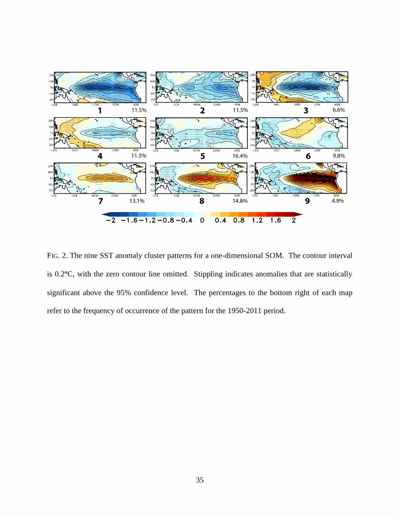
With K* determined, we now examine the nine SOM cluster patterns of tropical Pacific 263

SST anomalies. Figure 2 presents these nine patterns for the one-dimensional SOM. Because of 264

the topological ordering by the SOM, similar patterns are similarly numbered. Figure 2 reveals 265

three moderate to strong La Niña-like patterns (patterns 1-3), two weak La Niña-like patterns 266

(patterns 4-5), two weak CP El Niño-like patterns (patterns 6-7), a moderate CP/EP El Niño-like 267

pattern (pattern 8) and a strong EP El Niño-like pattern (pattern 9). In addition to amplitude, the 268

2 If a SOM cluster has only a single member, then (1) is undefined, and the distinguishability test cannot be

conducted. Therefore, in cases where a cluster only has one member, all pairs that include that particular cluster are

automatically assigned as statistically indistinguishable.

13

La Niña-like patterns most significantly distinguish themselves by the longitude of maximum 269

equatorial cooling and by the presence of weak (pattern 1), negative (patterns 2 and 5), or 270

positive (patterns 3 and 4) western Pacific SST anomalies. The El Niño-like patterns also 271

distinguish themselves by amplitude and the longitude of maximum equatorial SST anomalies, 272

but the western Pacific SST anomalies are similar for each El Niño-like pattern. Pattern 9 273

resembles the canonical EP El Niño, whereas pattern 8 seemingly represents a hybrid EP/CP El 274

Niño pattern, with maximum warming in the central Pacific, but a tongue of positive SST 275

anomalies that extends to the South American coast. Together, these nine SST patterns represent 276

the ENSO SST continuum. 277

As mentioned above, each September – February SST field is assigned to the best-278

matching SOM pattern on the basis of minimum Euclidean distance. The frequency of 279

occurrence of each SOM pattern is indicated to the bottom right of each map, revealing that most 280

patterns occur with similar frequency. To verify that these nine patterns do, in fact, resemble the 281

seasonal SST fields that comprise the clusters, centered pattern correlations (e.g., Santer et al. 282

1993) between each SST field and its corresponding best-matching SOM pattern are calculated. 283

The mean pattern correlation is 0.76, which confirms the close resemblance between these nine 284

patterns and the individual constituent SST anomaly fields of each cluster. 285

286

b. Changes in frequency distribution within the ENSO continuum 287

288

Next we examine how the frequency of occurrence of these nine SOM patterns has varied 289

over the past 60 years and how these changes in frequency have influenced the long-term 290

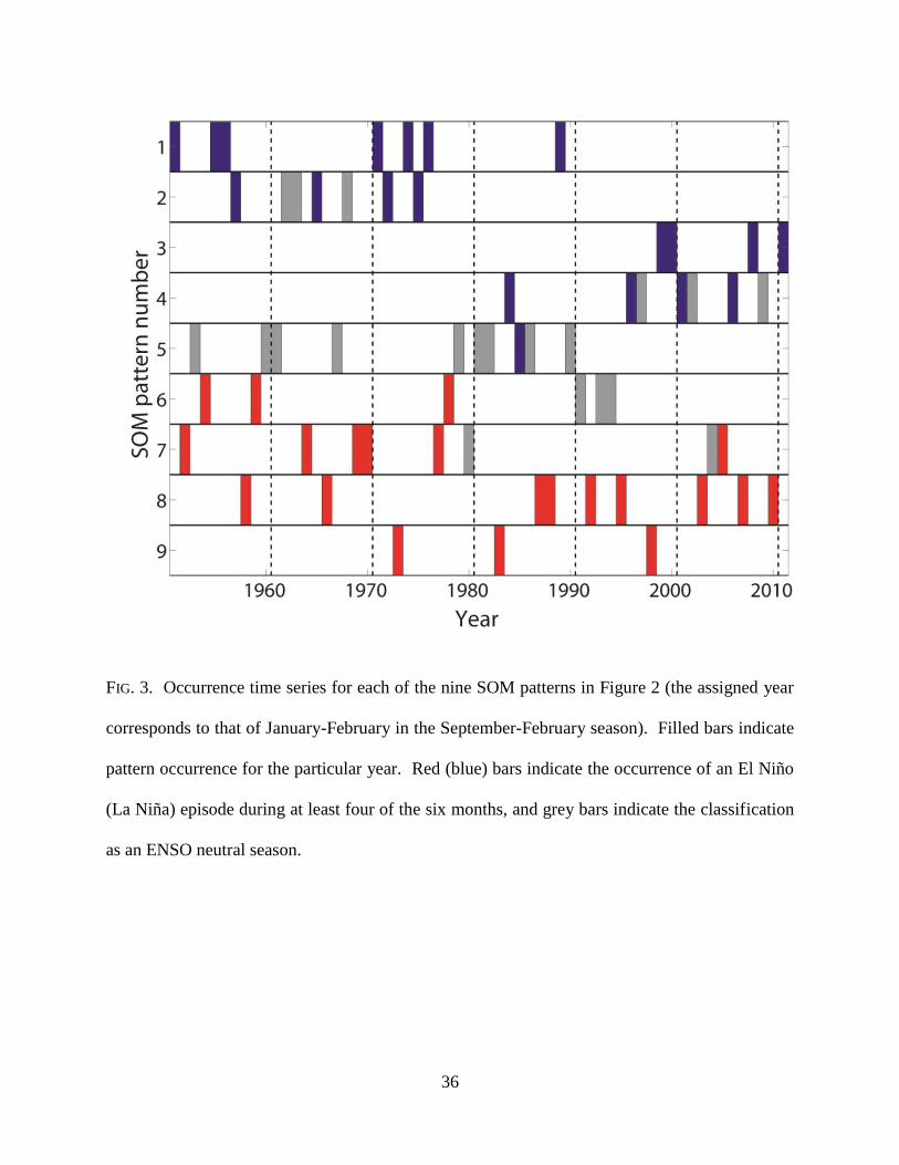
tropical Pacific SST trends. Figure 3 illustrates the occurrence time series for each of the nine 291

14

patterns. This plot demonstrates that each SOM pattern generally occurs for a single season and 292

for no more than two consecutive years. In addition, Figure 3 indicates whether at least four of 293

the six months in the September through February season are classified as an El Niño or La Niña 294

episode by NOAA CPC. NOAA CPC classifies an El Niño (La Niña) episode when the three-295

month running mean Niño 3.4 SST anomaly is greater than 0.5ᵒC (less than -0.5ᵒC) for at least 296

five consecutive overlapping, three-month seasons. Figure 3 confirms that patterns 1-4 are 297

closely associated with La Niña episodes, and patterns 6-9 are tied to El Niño episodes. Pattern 298

5 generally occurs when neutral ENSO conditions are declared. The CP El Niño episodes noted 299

in previous literature (e.g., Kug et al. 2009) generally correspond with SOM patterns 6 (e.g, 300

1977/78 and 1990/91), 7 (e.g., 2004/05), or 8 (e.g., 1994/95 and 2002/03). The only clearly 301

defined EP El Niño pattern, SOM pattern 9, corresponds with the strong El Niño episodes of 302

1972/73, 1982/83, and 1997/98. This observation that recent strong El Niño episodes have 303

strongly positive SST anomalies centered in the eastern Pacific, but that all other El Niño 304

episodes are centered over a broad range of longitudes is consistent with the recent studies of 305

Giese and Ray (2011) and Ray and Giese (2012). 306

Perhaps the most striking feature of Fig. 3 is the obvious trend in patterns 1-4, with 307

patterns 1 and 2 prevalent early in the period but nearly absent in the second half of the period, 308

and patterns 3 and 4 prevalent only after the mid 1990s. This trend represents a transition from 309

La Niña-like patterns with weak or negative SST anomalies in the western Pacific warm pool 310

(patterns 1 and 2) to La Niña-like patterns with positive SST anomalies in the western Pacific 311

warm pool (patterns 3 and 4). 312

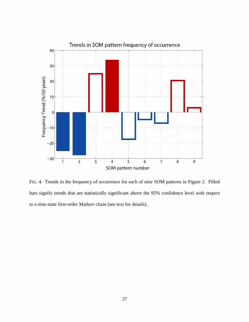
This transition is demonstrated more clearly in Figure 4, which shows the trend in the 313

frequency of occurrence for each SOM pattern. Statistical significance is assessed with respect 314

15

to a K-state first-order Markov chain, as determined through a Monte Carlo test similar to that of 315

Riddle et al. (2012). For this test, 10,000 synthetic first-order Markov chain SOM pattern 316

occurrence time series (like that of Fig. 3) are generated with the same transition probabilities as 317

observed. For each synthetic time series the trend in pattern frequency of occurrence is 318

calculated. Observed trends that are greater than the 97.5th

or less than the 2.5th

percentile of the 319

synthetic trends are deemed statistically significant above the 95% confidence level. Figure 4 320

confirms that the trends in SOM patterns 1-4 are strongest, with only the trend in pattern 3 falling 321

just short of statistical significance. Although flavors of El Niño have received more focus than 322

those of La Niña, none of the trends in the El Niño-like patterns (patterns 6-9) is statistically 323

significant over the past 60 years. 324

To determine how these SOM pattern frequency trends have contributed to the total 325

tropical Pacific SST trends, we calculate the SOM-derived trend as 326

(4) 327

where

is the frequency trend of SOM pattern i, and SSTi is SOM pattern i. Figure 5 presents 328

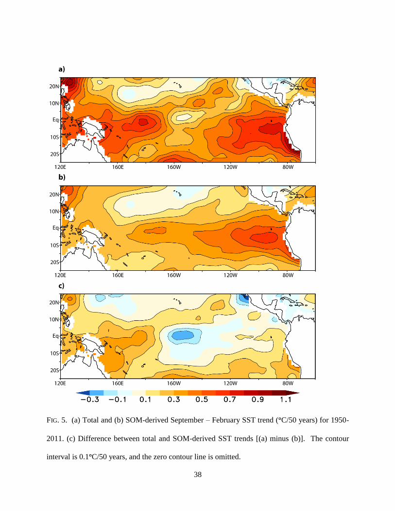
the total and SOM-derived September – February SST trends over the tropical Pacific region. 329

The total SST trend (Fig. 5a) reveals warming over the past 60 years over almost the entire 330

domain, but the most pronounced warming is indicated over the eastern equatorial Pacific and 331

western Pacific warm pool. The trend derived from (4) (Fig. 5b) also shows warming over most 332

of the domain, but the warming is most pronounced only over the eastern Pacific region. Figure 333

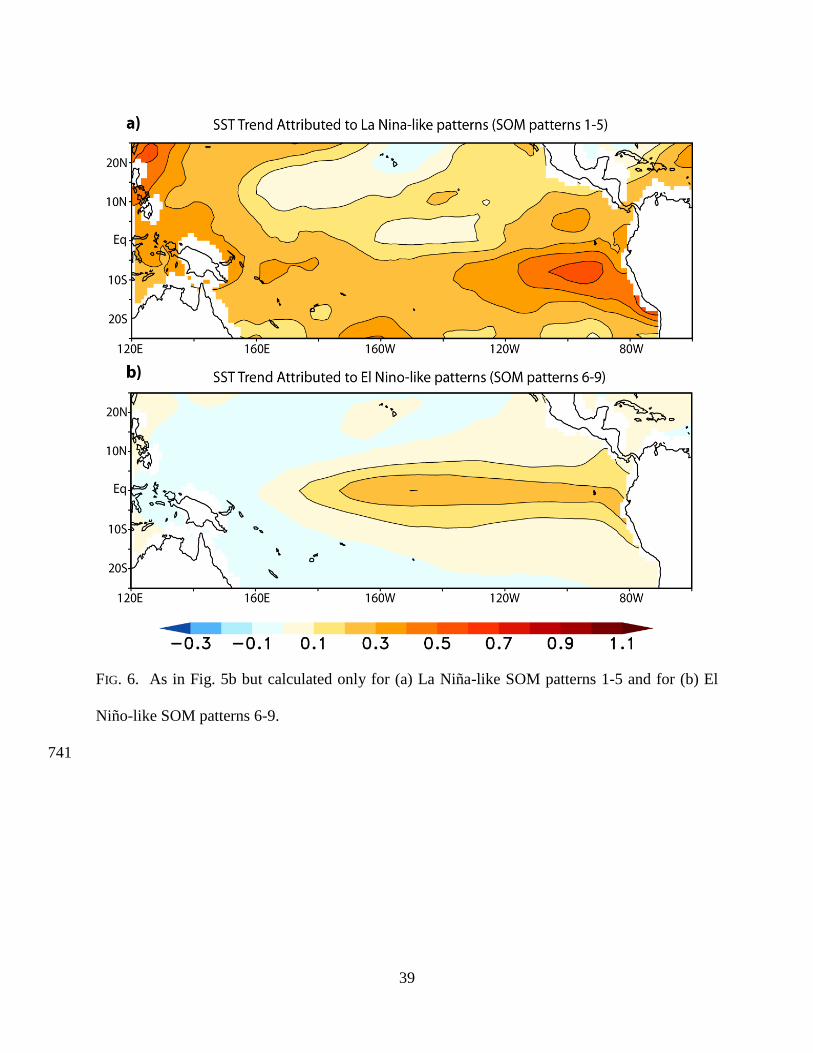
4 suggests that most of these ENSO flavor-related trends relate to changes in the frequency of La 334

Niña-like rather than El Niño-like patterns. This suggestion is confirmed in Fig. 6, which shows 335

the trends from the application of (4) only for La Niña-like SOM patterns 1-5 (Fig. 6a) and only 336

for El Niño-like SOM patterns 6-9 (Fig. 6b). The trend pattern derived solely from La Niña-like 337

16

pattern frequency changes (Fig. 6a) closely resembles the total ENSO-related trend pattern (Fig. 338

5b). The positive trends in El Niño-like pattern frequencies have contributed to modest warming 339

in the eastern equatorial Pacific region, but El Niño-related trends are weak throughout the rest 340

of the domain (Fig. 6b). 341

The difference between the total and SOM-derived trends (Fig. 5c) reveals generally 342

weak and even negative SST trends over the equatorial Pacific domain but with pronounced 343

positive trends remaining over the west Pacific warm pool. This result suggests that trends in the 344

frequency of occurrence of various ENSO flavors have dominated the SST trends in the eastern 345

equatorial Pacific region, but the trends in the west Pacific warm pool reflect a combination of 346

changes in frequency distribution and an additional superimposed long-term non-ENSO trend. 347

348

4. Discussion 349

The preceding analysis reveals nine statistically distinguishable patterns that represent the 350

ENSO continuum. This continuum perspective contrasts the framework of recent studies that 351

suggest two clearly distinct types of El Niño. This continuum perspective also is supported by 352

the recent work of Giese and Ray (2011), who find that the central longitude of El Niño SST 353

anomalies is not bimodal but rather is indistinguishable from a Gaussian distribution centered 354

near 140ᵒW. One notable observation is that the three strongest El Niño episodes of the past 60 355

years as measured by Niño 3.4 SST anomalies (1972/73, 1982/83, and 1997/98) feature strongest 356

SST anomalies in the eastern Pacific (SOM pattern 9). Perhaps the increased attention paid to 357

these strongest episodes has resulted in an over-emphasized sharpening of the differences 358

between EP and CP El Niño episodes. Evidence from an ocean reanalysis suggests that these 359

strong EP El Niño episodes may have resulted in an eastward bias of reconstructed El Niño SST 360

17

anomalies for periods before 1950 owing to the influence of these strong El Niño episodes on the 361

SST reconstructions (Giese and Ray 2011; Ray and Giese 2012). 362

The analysis also reveals that these nine ENSO flavors have made a significant 363

contribution to the long-term tropical Pacific SST trend through changes in their frequency 364

distribution (Fig. 5b). The most significant trends relate to the La Niña-like patterns, with the 365

dominance of patterns with negative western Pacific SST anomalies (patterns 1 and 2) before the 366

mid 1970s followed by the dominance of patterns with positive western Pacific SST anomalies 367

(patterns 3 and 4) after the mid 1970s, particularly from the mid 1990s to the present. These 368

frequency trends have contributed to tropical Pacific warming, particularly in the western Pacific 369

and eastern equatorial Pacific regions (Fig. 6a). One may hypothesize that this behavior reflects 370

a long-term warming trend most pronounced in the western Pacific warm pool superimposed on 371

interannual ENSO variability. However, this analysis suggests that there is a disproportionate 372

western Pacific warming for La Niña-like patterns, while there is no similar trend in the western 373

Pacific evident for the El Niño-like patterns3. In fact, the positive trend in the frequency of El 374

Niño-like patterns, particularly pattern 8, contributes to a weak negative SST trend in the west 375

Pacific warm pool region (Fig. 6b). Therefore, this analysis suggests that the simple paradigm of 376

a long-term trend superimposed on interannual variability, as typically assumed in global 377

warming attribution studies (e.g., Pall et al. 2011), may not be sufficient for understanding 378

tropical Pacific SST variability and trends. Rather, changes in the frequency distribution of 379

interannually varying patterns within the ENSO continuum, as depicted in Fig. 2, may impart a 380

significant contribution to the long-term trend. Moreover, recent theoretical work (Liang et al. 381

2012) proposes that the recent elevation in ENSO variance may be more of a cause than a 382

3 See Fig. 10 of L’Heureux et al. (2012) for additional evidence of enhanced west Pacific warm pool warming trends

in La Niña episodes relative to El Niño episodes during November – February.

18

consequence of eastern tropical Pacific warming, which would further underscore the difficulty 383

of separating interannual variability from the tropical mean state. 384

The trend toward La Niña-like patterns with positive SST anomalies in the western 385

Pacific warm pool is of particular interest because this general pattern may represent the “perfect 386

ocean for drought” over many midlatitude regions (Hoerling and Kumar 2003). This SST 387

pattern, captured by SOM patterns 3 and 4, dominated during the period between 1998 and 2002 388

(Fig. 3), which was a period of prolonged drought throughout much of the United States, 389

southern Europe, and Southwest Asia. Climate model simulations suggest that both the negative 390

SST anomalies in the eastern Pacific and positive SST anomalies in the western tropical Pacific 391

acted synergistically to force the persistent drought during this period (Hoerling and Kumar 392

2003; Lau et al. 2006). Figure 3 reveals that SOM patterns 3 and 4 occurred several additional 393

times since that period. In addition, there is evidence that the positive trend in Indo-Pacific 394

warm pool SSTs has contributed to changes in the wintertime teleconnection response to La 395

Niña, a trend toward a more zonally oriented circumglobal teleconnection pattern (Kumar et al. 396

2010; Lee et al. 2011). Given the widespread societal impacts of these particular La Niña 397

flavors, it is worthwhile for future studies to investigate whether the disproportionate warm pool 398

warming for La Niña-like patterns shall continue. 399

Both an EP (pattern 9) and CP/EP El Niño (pattern 8) SOM pattern also have experienced 400

positive trends in the frequency of occurrence over the past 60 years, but these trends are 401

indistinguishable from natural variability (Fig. 4). Given the recent focus on whether CP El 402

Niño episodes will become more frequent under global warming (Yeh et al. 2009), the positive 403

trend of CP El Niño-like SOM pattern 8 is of particular interest. However, the lack of a 404

significant trend is consistent with recent studies based on long integrations of a multivariate red 405

19

noise model (Newman et al. 2011b) and a coupled climate model (Yeh et al. 2011), which found 406

that the recent multidecadal increase in CP El Niño relative to EP El Niño episodes is consistent 407

with natural variability. 408

The changes in frequency of the ENSO flavor SOM patterns have contributed to an 409

overall positive SST trend in the central and eastern equatorial Pacific region (Fig. 5b), which is 410

consistent with recent findings linking positive equatorial Pacific trends to ENSO (Compo and 411

Sardeshmukh 2010; Lee and McPhaden 2010; L’Heureux et al. 2012). In addition, the increased 412

dominance of SOM patterns 3 and 4 at the expense of patterns 1 and 2 has contributed to the 413

warming trend in the tropical West Pacific region. The residual SST trend (Fig. 5c) reveals 414

positive SST trends in the western Pacific but weak or even negative SST trends throughout the 415

equatorial eastern Pacific region. Interestingly, this residual trend in Fig. 5c is somewhat similar 416

to the ENSO-unrelated SST trends obtained after applying a dynamic ENSO filter (Compo and 417

Sardeshmukh 2010; Solomon and Newman 2012). This particular filter, which accounts for the 418

SST evolution during ENSO and is obtained through a linear inverse modeling approach, reveals 419

a trend pattern of western Indo-Pacific warming and eastern equatorial Pacific cooling after the 420

trends associated with ENSO have been removed. The approach adopted here similarly shows 421

that ENSO-related trends have contributed to eastern equatorial Pacific warming (Fig. 5b), and 422

the residual SST warming is most pronounced in the west Pacific warm pool (Fig. 5c). 423

However, we must exercise caution when viewing long-term SST trends, given the data 424

uncertainties. In particular, a recent SST reconstruction based only on bucket SST and nighttime 425

marine surface air temperature measurements suggests less pronounced western Pacific warming 426

relative to that of the eastern Pacific (Tokinaga et al. 2012). Although beyond the scope of this 427

study, future research shall continue to investigate whether this enhanced western Pacific 428

20

warming is real, and, if so, whether it represents a response to anthropogenic warming (Clement 429

et al. 1996, Cane et al. 1997) or if enhanced equatorial Pacific warming, as in global climate 430

models (Collins et al. 2010; Xie et al. 2010), is more likely. The interplay between the potential 431

impact of greenhouse gas warming on ENSO (Guilyardi et al. 2009; Yeh et al. 2009; Collins et 432

al. 2010; Vecchi and Wittenberg 2010) and on long-term SST trends is a challenging problem, 433

but the approach presented here provides a possible framework for exploring this interaction. 434

435

5. Conclusions 436

This study opens with the question: how many ENSO flavors can we distinguish? To 437

address this question, we examine an approach that partitions tropical Pacific SST fields through 438

SOM analysis and then determines the maximum number of SOM cluster patterns that are 439

statistically distinguishable. This approach can be applied more generally to other cluster 440

analysis problems, particularly those of K-means cluster or SOM analysis, in order to answer the 441

recurring question of what is the optimal, or at least the maximum number of clusters to retain. 442

The approach adopted here has the appeal of being grounded in an accessible concept, statistical 443

distinguishability. Many other applications with serially correlated data would face the 444

additional challenge of accounting for serial correlation in the calculation of local p-values, but 445

the basic approach described here still would apply. 446

Although the present study focuses on seasonal SST patterns, ENSO also undergoes other 447

types of interdecadal variations, including changes in the seasonal evolution of ENSO-related 448

SST anomalies. Future extensions of this study may explore seasonal variations of ENSO 449

flavors. In addition, the dynamical processes responsible for these nine patterns remain an open 450

question. Through a multivariate red noise framework for tropical SST variability, Newman et 451

21

al. (2011a,b) find that the leading optimal structure corresponding with the EP ENSO is driven 452

by both surface and thermocline interactions, as in the classic “recharge-discharge” mechanism 453

(Jin 1997). In contrast, the optimal structure corresponding with CP ENSO evolves through non-454

local SST interactions, such as the advection of SST anomalies, but without the recharge-455

discharge mechanism. The CP ENSO event growth is more modest than that of the EP ENSO, 456

but the lack of a discharge mechanism allows the CP ENSO to decay more slowly (Newman et 457

al. 2011b). Because these two optimal initial structures are orthogonal, the framework of 458

Newman et al. (2011a,b) suggests a continuum of “mixed” CP/EP ENSO patterns with 459

intermediate dynamical characteristics. The analysis presented here is consistent with this 460

general framework, but additional work is needed. 461

The analysis presented here also suggests that although El Niño flavors often receive 462

more focus than those of La Niña in the literature, changes related to La Niña-like SST patterns 463

have made a stronger impact on long-term SST trends over the past 60 years. A number of 464

outstanding questions remain. Given that tropical Pacific SST anomalies have far-reaching 465

effects through tropical convection anomalies and the triggering of atmospheric teleconnections, 466

future research shall augment recent efforts (e.g., Larkin and Harrison 2005; Weng et al. 2007; 467

Mo 2010; Hu et al. 2012) to examine how many ENSO flavor teleconnections and remote 468

impacts can be distinguished. In addition, the various ENSO flavors within the ENSO 469

continuum and their relationship with the long-term SST trend remain an active area of research 470

(Guilyardi et al. 2009; Yeh et al. 2009; Collins et al. 2010; Liang et al. 2012). A unique set of 471

questions raised in this study relates to the trend toward La Niña-like patterns with enhanced 472

SST anomalies in the west Pacific warm pool. Why has there been disproportionate west Pacific 473

warming for La Niña patterns? Will this trend continue? Can coupled global climate models 474

22

capture this sort of variability? The approach presented here provides a framework for 475

examining the ENSO continuum and questions like these with a manageable set of representative 476

ENSO flavors. 477

478

Acknowledgments. 479

I sincerely thank Drs. Steven Feldstein, Sukyoung Lee, Jinbao Li, and Shang-Ping Xie for 480

thoughtful discussions and helpful comments that contributed to this work. I also thank Dr. Eli 481

Tziperman and two anonymous reviewers for constructive comments that improved the quality 482

of this study. I am grateful for support through a grant from the NOAA Climate Test Bed 483

program. NOAA ERSST V3 data are provided by the NOAA/OAR/ESRL PSD, Boulder, 484

Colorado, USA, from their Web site at http://www.esrl.noaa.gov/psd. 485

486

487

References 488

Ashok, K., S. K. Behera, S. A. Rao, H. Weng, and T. Yamagata, 2007: El Niño Modoki and its 489

possible teleconnection. J. Geophys. Res., 112, C11007, doi:10.1029/2006JC003798. 490

491

Benjamini, Y., and Y. Hochberg, 1995: Controlling the false discovery rate: A practical and 492

powerful approach to multiple testing. J. Roy. Stat. Soc., B57, 289-300. 493

494

Cane, M. A., A. C. Clement, A. Kaplan, Y. Kushnir, D. Pozdnyakov, R. Seager, S. E. Zebiak, 495

and R. Murtugudde, 1997: Twentieth-century sea surface temperature trends. Science, 275, 957-496

960. 497

23

498

Christiansen, B., 2007: Atmospheric circulation regimes: Can cluster analysis provide the 499

number?. J. Climate, 20, 2229–2250. 500

501

Chu, J.-E., S. N Hameed, and K.-J. Ha, 2012: Non-linear, intraseasonal phases of the East Asian 502

summer monsoon: Extraction and analysis using self-organizing maps. J. Climate, in press. 503

504

Collins, M., S.-I An, W. Cai, A. Ganachaud, E. Guilyardi, F.-F. Jin, M. Jochum, M. Lengaigne, 505

S. Power, A. Timmermann, G. Vecchi, and A. Wittenberg, 2010: The impact of global warming 506

on the tropical Pacific Ocean and El Niño. Nat. Geosci., 3, 391-397. 507

508

Compo, G. P., and P. D. Sardeshmukh, 2010: Removing ENSO-Related variations from the 509

climate record. J. Climate, 23, 1957–1978. 510

511

Deser, C., M. A. Alexander, S.-P. Xie, and A. S. Phillips, 2010: Sea surface temperature 512

variability: patterns and mechanisms. Ann. Rev. Mar. Sci., 2010.2, 115-143. 513

514

Folland, C., C. Anderson, 2002: Estimating changing extremes using empirical ranking methods. 515

J. Climate, 15, 2954–2960. 516

517

Freeman, L. A., A. J. Miller, R. D. Norris, and J. E. Smith, 2012: Classification of remote Pacific 518

coral reefs by physical oceanographic environment, J. Geophys. Res., 117, C02007, 519

doi:10.1029/2011JC007099. 520

24

521

Giese, B. S., and S. Ray, 2011: El Niño variability in simple ocean data assimilation (SODA), 522

1871-2008. J. Geophys. Res., 116, C02024, doi:10.1029/2010JC006695. 523

524

Guilyardi, E., A. Wittenberg, A. Fedorov, M. Collins, C. Wang, A. Capotondi, G. J. van 525

Oldenborgh, T. Stockdale, 2009: Understanding El Niño in ocean–atmosphere general 526

circulation models: Progress and challenges. Bull. Amer. Meteor. Soc., 90, 325–340. 527

528

Hastie, T., R. Tibshirani, and J. Friedman, 2009: Unsupervised learning. The Elements of 529

Statistical Learning: Data Mining, Inference, and Prediction, Springer, 485-585. 530

531

Hewitson, B.C., and R. G. Crane, 2002: Self-organizing maps: Applications to synoptic 532

climatology. Clim. Res., 22, 13-26. 533

534

Hoerling, M. P., and A. Kumar, 2003: The perfect ocean for drought. Science, 299, 691-694. 535

536

Hoerling, M. P., A. Kumar, and M. Zhong, 1997: El Niño, La Niña, and the nonlinearity of their 537

teleconnections. J. Climate, 10, 1769–1786. 538

539

Hu, Z.-Z., A. Kumar, B. Jha, W. Wang, B. Huang, and B. Huang, 2012: An analysis of warm 540

pool and cold tongue El Niños: air-sea coupling processes, global influences, and recent trends. 541

Climate Dyn., in press, doi:10.1007/s00382-011-1224-9. 542

543

25

Jin, B., G. Wang, Y. Liu, and R. Zhang, 2010: Interaction between the East China Sea Kuroshio 544

and the Ryukyu Current as revealed by the self-organizing map, J. Geophys. Res., 115, C12047, 545

doi:10.1029/2010JC006437. 546

547

Jin, F.-F., 1997: An equatorial ocean recharge paradigm for ENSO. Part I: Conceptual model. J. 548

Atmos. Sci., 54, 811-829. 549

550

Johnson, N. C., and S. B. Feldstein, 2010: The continuum of North Pacific sea level pressure 551

patterns: Intraseasonal, interannual, and interdecadal variability. J. Climate, 23, 851–867. 552

553

Johnson, N. C., S. B. Feldstein, and B. Tremblay, 2008: The continuum of Northern Hemisphere 554

teleconnection patterns and a description of the NAO Shift with the use of self-organizing maps. 555

J. Climate, 21, 6354–6371. 556

557

Johnson, N. C., and S.-P. Xie, 2010: Changes in the sea surface temperature threshold for 558

tropical convection. Nat. Geosci., 3, 842-845. 559

560

Larkin, N. K, and D. E. Harrison, 2005: Global seasonal temperature and precipitation anomalies 561

during El Niño. Geophys. Res. Lett., 32, L16705, doi:10.1029/2005GL022860. 562

563

Leloup, J., Z. Lachkar, J.-P. Boulanger, and S. Thiria, 2007: Detecting decadal changes in ENSO 564

using neural networks. Climate Dyn., 28, 147-162, doi:10.1007/s00382-006-0173-1. 565

566

26

Kao, H.-Y., and J.-Y. Yu, 2009: Contrasting eastern-Pacific and central-Pacific types of ENSO. 567

J. Climate, 22, 615-632. 568

569

Kohonen, T., 2001: Self-Organizing Maps. Springer, 501. 570

571

Kug, J.-S., F.-.F. Jin, and S.-I. An, 2009: Two types of El Niño events: Cold tongue El Niño and 572

warm pool El Niño. J. Climate, 22, 1499-1515. 573

574

Kumar, A., B. Jha, and M. L’Heureux, 2010: Are tropical SST trends changing the global 575

teleconnection during La Niña? Geophys. Res. Lett., 37, L12702, doi:10.1029:2010GL043394. 576

577

Lau, N.-C., A. Leetmaa, M. J. Nath, and H.-L. Wang, 2006: Attribution of atmospheric 578

variations in the 1997-2003 period to SST anomalies in the Pacific and Indian Ocean basins. J. 579

Climate, 19, 3607-3628. 580

581

Lee, S., T. Gong, N. Johnson, S. B. Feldstein, and D. Pollard, 2011: On the possible link between 582

tropical convection and the Northern Hemisphere Arctic surface air temperature change between 583

1958 and 2001. J. Climate, 24, 4350–4367. 584

585

Lee, T., and M. J. McPhaden, 2010: Increasing intensity of El Niño in the central-equatorial 586

Pacific. Geophys. Res. Lett., 37, L14603, doi:10.1029/2010GL044007. 587

588

27

L’Heureux, M. L., D. C. Collins, and Z.-Z. Hu, 2012: Linear trends in sea surface temperature of 589

the tropical Pacific Ocean and implications for the El Niño-Southern Oscillation. Climate Dyn., 590

in press, doi:10.1007/s00382-012-1331-2. 591

592

Liang, J., X.-Q. Yang, and D.-Z. Sun, 2012: The effect of ENSO events on the tropical Pacific 593

mean climate: Insights from an analytical model. J. Climate, 25, 7590-7606. 594

595

Liu, Y., R. H. Weisberg, and C. N. K. Mooers, 2006: Performance evaluation of the self-596

organizing map for feature extraction. J. Geophys. Res., 111, C05018, 597

doi:10.1029/2011GL047658. 598

599

Livezey, R. E., and W. Y. Chen, 1983: Statistical field significance and its determination by 600

Monte Carlo techniques. Mon. Wea. Rev., 111, 46-59. 601

602

Ma, J., S.-P. Xie, and Y. Kosaka, 2012: Mechanisms for tropical tropospheric circulation change 603

in response to global warming. J. Climate, 25, 2979-2993. 604

605

Michelangeli, P.-A., R. Vautard, and B. Legras, 1995: Weather regimes: Recurrence and quasi 606

stationarity. J. Atmos. Sci., 52, 1237–1256. 607

608

Newman M., M. A. Alexander, and J. D. Scott, 2011a: An empirical model of tropical ocean 609

dynamics. Climate Dyn., 37, 1823-1841. 610

611

28

Newman, M., S.-I. Shin, and M. A. Alexander, 2011b: Natural variation in ENSO flavors. 612

Geophys. Res. Lett., 38, L14705, doi:10.1029/2011GL047658. 613

614

Pall, P., T. Aina, D. A. Stone, P. A. Stott, T. Nozawa, A. G. J. Hilberts, D. Lohmann, and M. R. 615

Allen, 2011: Anthropogenic greenhouse gas contribution to flood risk in England and Wales in 616

autumn 2000. Nature, 470, 382-385. 617

618

Ray, S., and B. S. Giese, 2012: Historical changes in El Niño and La Niña characteristics in an 619

ocean reanalysis. J. Geophys. Res., 117, C11007, doi:10.1029/2012JC008031. 620

621

Riddle E. E., M. B. Stoner, N. C. Johnson, M. L. L’Heureux, D. C. Collins, and S. B. Feldstein, 622

2012: The impact of the MJO on clusters of wintertime circulation anomalies over the North 623

American region. Climate Dyn., in press, doi:10.1007/s00382-012-1493-y. 624

625

Rodgers, K. B., P. Friederichs, and M. Latif, 2004: Tropical Pacific decadal variability and its 626

relation to decadal modulation of ENSO. J. Climate, 17, 3761-3774. 627

628

Reusch, D. B., R. B. Alley, and B. C. Hewitson, 2005: Relative performance of self-organizing 629

maps and principal component analysis in pattern extraction from synthetic climatological data. 630

Polar Geogr., 29, 227-251. 631

632

Richardson, A. J., C. Risien, and F. A. Shillington, 2003: Using self-organizing maps to identify 633

patterns in satellite imagery. Prog. Oceanog., 59, 223-239. 634

29

635

Ropelewski, C. F., M. S. Halpert, 1987: Global and regional scale precipitation patterns 636

associated with the El Niño/Southern Oscillation. Mon. Wea. Rev., 115, 1606–1626. 637

638

Santer, B. D., T. M. L. Wigley, and P. D. Jones, 1993: Correlation methods in fingerprint 639

detection studies. Climate Dyn., 8, 265-276. 640

641

Shin, S.-I., and P. D. Sardeshmukh, 2011: Critical influence of the pattern of tropical ocean 642

warming on remote climate trends. Climate Dyn., 36, 1577-1591. 643

644

Smith, T.M., R.W. Reynolds, T. C. Peterson, and J. Lawrimore, 2008: Improvements to NOAA's 645

Historical Merged Land-Ocean Surface Temperature Analysis (1880-2006). J. Climate, 21, 646

2283-2296. 647

648

Solomon, A., and M. Newman, 2012: Reconciling disparate twentieth-century Indo-Pacific 649

ocean temperature trends in the instrumental record. Nature Climate Change, 650

doi:10.1038/NCLIMATE1591. 651

652

Tokinaga, H., S.-P. Xie, C. Deser, Y. Kosaka, and Y. M. Okumura, 2012: Slowdown of the 653

Walker circulation driven by tropical Indo-Pacific warming. Nature, 491, 439-443. 654

655

Trenberth, K. E., and J. M. Caron, 2000: The Southern Oscillation revisited: sea level pressures, 656

surface temperatures, and precipitation. J. Climate, 13, 4358-4365. 657

30

658

Trenberth, K. E., and D. P. Stepaniak, 2001: Indices of El Niño. J. Climate, 14, 1697-1701. 659

660

Vecchi, G.A. and A.T. Wittenberg, 2010: El Niño and our future climate: where do we stand? 661

WIREs Clim. Change, 1, 260-270. 662

663

Vesanto, J., J. Himberg, E. Alhoniemi, and J. Parhankangas, 2000: SOM toolbox for Matlab 5. 664

Helsinki University of Technology, Finland. [Available online at 665

http://www.cis.hut.fi/projects/somtoolbox/.] 666

667

Weng, H., K. Ashok, S. K. Behera, S. A. Rao, and T. Yamagata, 2007: Impacts of recent El Niño 668

Modoki on dry/wet conditions in the Pacific Rim during boreal summer. Climate Dyn., 29, 113-669

129. 670

671

Xie, S.-P., C. Deser, G. A. Vecchi, J. Ma, H. Teng, and A. T. Wittenberg, 2010: Global warming 672

pattern formation: Sea surface temperature and rainfall. J. Climate, 23, 966–986. 673

674

Xue, Y., T. M. Smith, and R. W. Reynolds, 2003: Interdecadal changes of 30-yr SST normals 675

during 1871-2000. J. Climate, 16, 1601-1612. 676

677

Yeh, S.-W, B. K. Kirtman, J.-S. Kug, W. Park, and M. Latif, 2011: Natural variability of the 678

central Pacific El Niño event on multi-centennial timescales. Geophys. Res. Lett., 38, L02704, 679

doi:10.1029/2010GL045886. 680

681

31

Yeh, S.-W., J.-S. Kug, B. Dewitte, M.-H. Kwon, B. P. Kirtman, and F.-F. Jin, 2009: El Niño in a 682

changing climate. Nature, 461, 511-514. 683

684

Yu, J.-Y., and S. T. Kim, 2011: Relationships between extratropical sea level pressure variations 685

and the central Pacific and eastern Pacific types of ENSO. J. Climate, 24, 708-720. 686

687

Wilks, D. S., 2006: On “field significance” and the false discovery rate. J. Appl. Meteor. 688

Climatol., 45, 1181-1189. 689

690

691

692

693

694

695

696

697

698

699

700

701

702

703

704

32

List of Figures 705

FIG. 1. The number of SOM SST cluster pattern pairs that are statistically indistinguishable at the 706

95% confidence level as a function of the number of SOM patterns, K. 707

708

FIG. 2. The nine SST anomaly cluster patterns for a one-dimensional SOM. The contour interval 709

is 0.2ᵒC, with the zero contour omitted. Stippling indicates anomalies that are statistically 710

significant above the 95% confidence level. The percentages to the bottom right of each map 711

refer to the frequency of occurrence of the pattern for the 1950-2011 period. 712

713

FIG. 3. Occurrence time series for each of the nine SOM patterns in Figure 2 (the assigned year 714

corresponds to that of January-February in the September-February season). Filled bars indicate 715

pattern occurrence for the particular year. Red (blue) bars indicate the occurrence of an El Niño 716

(La Niña) episode during at least four of the six months, and grey bars indicate the classification 717

as an ENSO neutral season. 718

719

FIG. 4. Trends in the frequency of occurrence for each of nine SOM patterns in Figure 2. Filled 720

bars signify trends that are statistically significant above the 95% confidence level with respect 721

to a nine-state first order Markov chain (see text for details). 722

723

FIG. 5. (a) Total and (b) SOM-derived September – February SST trend (ᵒC/50 years) for 1950-724

2011. (c) Difference between total and SOM-derived SST trends [(a) minus (b)]. The contour 725

interval is 0.1ᵒC/50 years, and the zero contour line is omitted. 726

727

33

FIG. 6. As in Fig. 5b but calculated only for (a) La Niña-like SOM patterns 1-5 and for (b) El 728

Niño-like SOM patterns 6-9. 729

730

731

732

733

734

735

736

737

738

739

740

34

FIG. 1. The number of SOM SST cluster pattern pairs that are statistically indistinguishable at the

95% confidence level as a function of the number of SOM patterns, K.

35

FIG. 2. The nine SST anomaly cluster patterns for a one-dimensional SOM. The contour interval

is 0.2ᵒC, with the zero contour line omitted. Stippling indicates anomalies that are statistically

significant above the 95% confidence level. The percentages to the bottom right of each map

refer to the frequency of occurrence of the pattern for the 1950-2011 period.

36

FIG. 3. Occurrence time series for each of the nine SOM patterns in Figure 2 (the assigned year

corresponds to that of January-February in the September-February season). Filled bars indicate

pattern occurrence for the particular year. Red (blue) bars indicate the occurrence of an El Niño

(La Niña) episode during at least four of the six months, and grey bars indicate the classification

as an ENSO neutral season.

37

FIG. 4. Trends in the frequency of occurrence for each of nine SOM patterns in Figure 2. Filled

bars signify trends that are statistically significant above the 95% confidence level with respect

to a nine-state first-order Markov chain (see text for details).

38

FIG. 5. (a) Total and (b) SOM-derived September – February SST trend (ᵒC/50 years) for 1950-

2011. (c) Difference between total and SOM-derived SST trends [(a) minus (b)]. The contour

interval is 0.1ᵒC/50 years, and the zero contour line is omitted.

39

FIG. 6. As in Fig. 5b but calculated only for (a) La Niña-like SOM patterns 1-5 and for (b) El

Niño-like SOM patterns 6-9.

741