07-074

Copyright © 2007, 2008 by Eric Werker, Faisal Z. Ahmed, Charles Cohen

Working papers are in draft form. This working paper is distributed for purposes of comment and discussion only. It may not be reproduced without permission of the copyright holder. Copies of working papers are available from the author.

How is Foreign Aid Spent? Evidence from a Natural Experiment Eric Werker Faisal Z. Ahmed Charles Cohen

How is Foreign Aid Spent? Evidence from a Natural Experiment

By ERIC WERKER, FAISAL Z. AHMED, AND CHARLES COHEN∗

July 2008

Abstract We use oil price fluctuations to construct a new instrument to test the

impact of transfers from wealthy OPEC nations to their poorer Muslim allies. The instrument identifies plausibly exogenous variation in foreign aid. We investigate how aid is spent by tracking its short-run effect on aggregate demand, the national accounts, and the balance of payments. Aid has no measurable impact on prices or economic growth, though it does affect most components of the national income accounts. We find that much aid is consumed, primarily in the form of imported non-capital goods. Aid substitutes for domestic savings, has no effect on the financial account, and leads to unaccounted capital flight.

∗ Eric Werker, Harvard Business School, Boston MA, 02163, ewerker@hbs.edu; Faisal Z. Ahmed, University of Chicago, faisal@uchicago.edu; Charles Cohen, Sankaty Advisors, ccohen@sankaty.com. We would like to thank Alberto Alesina, Laura Alfaro, Andreea Balan, Abhijit Banerjee, Olivier Blanchard, Francesco Caselli, Santanu Chatterjee, Edward Glaeser, Michael Kremer, David Roodman, two anonymous referees, and participants at the Harvard Development Workshop, New England Universities Development Consortium, and Center for Global Development for valuable comments and suggestions. The usual caveat applies.

1

It is notoriously difficult to measure the causal impact of foreign aid on the economy. The

“micro-macro paradox” (Mosley 1986) renders it impossible to add up the effects of individual

aid projects, since foreign aid is fungible. Thus, researchers are left to conduct cross-country

analyses to capture the effect of aid on economic growth and other outcomes, net of the recipient

governments’ domestic budget reshuffling. This large literature has produced mixed results and

much disagreement, largely due to different interpretations over causal inference (Roodman

2007). After all, since donors may reward countries for good performance—or bail out basket

cases—concerns of endogeneity are justified. Not surprisingly, the literature has employed a

number of instrumentation strategies (see Rajan and Subramanian, forthcoming).

Existing instrumental-variable approaches use the literature on the determinants of aid

(e.g. Alesina and Dollar 2000) to isolate variables that predict foreign aid, broadly, and then use

the best candidates to predict aid in a two-stage aid-on-growth regression. But each existing

instrument for aid (see Boone 1996; Hansen and Tarp 2001) can be criticized for one of three

broad reasons: one, it is highly collinear with aid itself (e.g. lagged aid, lagged aid squared); two,

it stands a good chance of not being truly exogenous to the economy (e.g. lagged arms imports,

lagged “policy”, lagged GDP per capita, policy interactions); or three, it is basically time-

invariant and thus limits the temporal inferences that can be drawn from the analysis (e.g. Egypt,

Africa Franc zone, population).

In this paper, we undertake a very different attempt to purge endogeneity concerns from

the cross-country regressions. Rather than rely on a broad determinant of foreign aid to isolate

exogenous variation, we focus on a specific episode of foreign aid and instrument for aid using a

natural experiment approach. In particular, we track the economic impact of what may be the

most significant foreign aid windfall since the Marshall Plan.

The twin oil crises of 1973 and 1979 produced over a decade of sky-high oil prices,

which filled the government coffers of Gulf oil exporters. These nations, principally Saudi

Arabia, the United Arab Emirates, and Kuwait, then turned around and distributed some of the

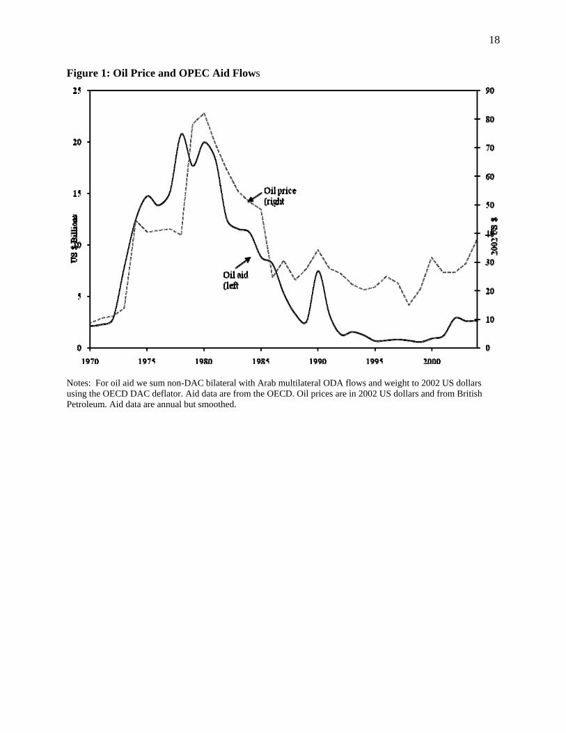
rents to countries in the developing world (Neumayer 2002) as depicted in Figure 1. Arab donors

were generous with their foreign aid, donating over 1.5 percent of their GDP (Neumayer 2003).

2

Not surprisingly, the aid heavily favored Muslim countries.1 In contrast to most aid today, this

aid was largely unconditional block grants to finance ministries (Hallwood and Sinclair 1981;

Hunter 1984). Together, these facts imply that poor, Muslim countries received a windfall in

unconditional foreign aid coincident with the rise in the price of oil.

This natural experiment approach is uniquely powerful among instrumental variable

approaches to measure the short-run impact of aid on the economy. This question represents a

significant gap in our understanding of the macroeconomic effects of aid. With all the attention

on aid and growth, there has been relatively little focus on what one would actually expect to

occur in a normal economy upon receipt of foreign assistance. For instance, foreign aid should

not show up in gross domestic product in and of itself – after all, it is not produced inside a

country's borders. However, if a reasonable fraction of it is spent inside the country, it should

eventually appear in the national accounts, whether or not a country is corrupt or mismanaged.

Yet we have very little understanding of how foreign aid trickles through the economy.

Since we are interested in the short-run impact of aid on macroeconomic activity, the

price of oil may be correlated with the outcome variables we are evaluating. But we can

incorporate the fact that OPEC aid heavily favored Muslim countries. Although oil prices may

directly affect the outcome variables of interest, they should not differentially affect these

outcomes in Muslim countries. Hence, we can use interaction of the price of oil with whether the

recipient country is Muslim as an instrument for foreign aid.

Our instrument allows for the inclusion of country fixed effects, which eliminates omitted

variable bias due to unobservable time-invariant country effects, as well time fixed effects that

account for global shocks. Moreover, the flow of other funds (principally workers’ remittances

and private charity) originating from oil exporters that are potentially correlated with our

instrument do not seem to constitute an important threat to the validity of the empirical strategy,

as we show in various robustness checks.

Using this empirical approach, we examine the short-run effect of foreign aid on

aggregate demand, including real GDP growth, inflation, and real exchange rate appreciation.

We then explore how the aid windfall was spent by tracking the impact of aid on the national

accounts. Finally, we investigate the impact of aid on domestic savings and the financial account.

1 Neumayer (2003) performs a Heckman estimation of aid receipts from Arab donors as many countries receive no aid at all from these donors. The only two significant variables at the gate-keeping stage and the level stage, other than the size of population, are whether the recipient country is Arab and/or Muslim.

3

The results are informative. We find little effect on growth, domestic prices, or the real

exchange rate. However, there is some evidence that all the components of GDP, including

government spending and investment, may have been affected. Consumption, specifically of

imports, rises substantially. For each percentage point of GDP in additional foreign aid,

household consumption rises by at least 0.6 percent of GDP, and imports increase by around 1

percent of GDP. Non-capital imports appear to rise faster than capital imports. Aid substitutes

approximately one-for-one for domestic savings and brings little in the way of foreign

investment. Finally, contrary to anecdotes of Arab charity flooding into poor Muslim countries,

the aid was associated with huge unaccounted capital outflows on the balance of payments.

The rest of the paper is organized as follows. Section I explains the empirical

specification and data. Section II describes our results. Section III subjects the findings to various

robustness checks. Section IV concludes.

I. Specification and Data

Our empirical setup involves the standard aid-on-growth specification with fixed effects,

taking advantage of the two stage least squares (2SLS) setup:

(1) Aidit = α + β*Muslimi*p(oil)t + δ*Xit + λ*Di + ζ*Dt + εit

(2) yi,t = a + b* Aidit + c*Xit + d*Di + e*Dt + uit

where i indexes countries, t indexes years, Muslim is a dummy variable indicating whether at

least 70 percent of the country’s population identifies with the Islamic religion, p(oil) is the price

of oil, X is a vector economic, political, and demographic controls for each country, and D is a

vector of country and year fixed effects. Aid is expressed as a percentage of GDP, and y is the

outcome variable of interest—e.g. economic growth, or consumption as a percentage of GDP.

Unless otherwise specified, all data are from the World Development Indicators 2005

database from the World Bank and include all available observations from 1960-2003. Likewise,

our analysis excludes rich countries (classified as high income by the World Bank) and oil

producers (classified by British Petroleum (2005)). Rich countries do not receive development

4

assistance, and for Muslim oil-producing developing countries, the impact of high oil prices will

have a direct impact on the economy that dwarfs any increase in foreign aid. Appendix A lists

the countries that are included.

We choose standard controls that should not introduce unnecessary endogeneity into the

aid/economy relationship. The controls are real GDP per capita (poor countries receive more

aid), log of population (aid is biased towards smaller countries), lagged growth in GDP per

capita, and the occurrence of war within the country (both of which may have a first-order effect

on the economy independent of aid). As we include dummy variables for year and country as

part of our fixed effects specification, it is not necessary to introduce any other spatial or

temporal dummies such as world regions, ethnolinguistic fractionalization, or Cold War era.

Further details on the all the included variables and their summary statistics are available in

Appendices B and C.

As we are interested in the short-run effects of aid on the economy, we estimate

regressions using annual data as well as data averaged over intervals of 4 years. These periods

(1960-1963, 1964-1967, etc.) are intended to help smooth some fluctuations in both the

independent and dependent variables, but still effectively account for the heterogeneity in our

instrument over time. For the annual frequency data we estimate our initial set of regressions

using Newey-West standard errors that allow for autocorrelation up to one lag period. We

estimate our 4-year averaged regressions using ordinary least squares (OLS) with Huber-White

standard errors.

II. Results

A. First stage

Table 1 reports the results of the first stage regression. Column 1 describes the effect of

oil prices on the amount of foreign aid received by non-oil producer Muslim countries. The

coefficient on aid is 0.116 which means that an increase in the price of oil by $10 provides a

windfall of foreign aid to non-oil producer Muslim countries equal to 1.16 percent of GDP. The

control variables have the expected signs: richer and more populous countries receive less aid

(as a percent of GDP), countries at war receive less aid, and growth is insignificant. The F-test on

5

the instrument yields a value of 28.3 easily exceeding the threshold for weak instruments of 10

suggested by Staiger and Stock (1997).

The instrument performs reasonably well in the regressions using data averaged over 4

years. An increase in the price of oil by $10 provides an average windfall of foreign aid to non-

oil Muslim countries equal to 1.1 percent of GDP. The control variables jump around somewhat,

and the F-test on the instrument (13.1) exceeds the threshold for weak instruments. The strength

of the first stage regression at both annual and 4-year frequencies allows us to run two stage least

squares on a variety of outcome variables, though the lower F-statistic on the 4-year data warns

of noisier results on the pooled data.

To confirm that these effects are being driven through aid and not GDP we rerun the

specifications in columns 1 and 2 on aid per capita. While the F-statistics are weaker than in the

first two columns, the instrument retains strong predictive power. A $10 increase in the price of

oil is associated with more than eight dollars additional aid per capita to Muslim non-oil

producers.

The chief concern with the instrumentation strategy is that it will pick up not only

government-to-government aid from Gulf states to poor Muslim countries, but private financial

flows as well—in particular, workers’ remittances and private charity. Ex ante, there is no reason

to doubt that salaries getting sent home from Muslim workers in the oilfields, or Wahabbi charity

from Saudi Arabia to Muslim communities in the Sahel, might be substantial. (Interestingly, this

phenomenon may plague other papers estimating the economic impact of foreign aid, but the

concern has not been raised in the literature.)

There are no direct data available on private charity, but we test for these flows using

balance of payments data in sub-section E, where we find little evidence that private charity

flows are any concern for the estimation strategy. For workers’ remittances, using data from the

IMF (with unfortunately limited coverage during the 1970s), we follow a two-part approach.

First, we re-run the first-stage regression with workers’ remittances, then remittances combined

with aid, as outcome variables. With this exercise we find that the aid windfall picked up by the

instrument dwarfs any remittance windfall. Second, in section III B we re-run our main results

controlling for workers’ remittances as well as instrumenting for a combined aid plus

remittances. This exercise changes the magnitudes of some of the estimations but does not alter

our qualitative conclusions.

6

Column 5 of Table 1 regresses workers’ remittances on the instrument. As can be seen,

the magnitude of the coefficient (0.022) is less than one sixth that of the coefficient when

combined remittances plus aid are regressed on the instrument (0.139) in column 6. So it appears

that an increase in remittances is being picked up by the instrument, but also that the aid windfall

dominates any remittance windfall. This should not be surprising for two reasons. One, there is

no reason to suspect that the oil companies would have raised wages one-for-one with oil prices;

likely, the companies and the state would keep most of the rents. Two, while there are many

workers in the Gulf from primarily Muslim countries, there are also many from countries we do

not classify as Muslim, like the Philippines. Given these results, and the limitations that

including the remittance data imposes on the sample size, we proceed through our main results

without controlling for remittances, but recognizing that we may be overestimating some

coefficients.

B. Aggregate Demand, Inflation, and the Real Exchange Rate

A transfer of funds from one country to another raises the recipient government’s level of

available funds. If spent, an inflow of aid should provide an economic stimulus, representing an

outward shift in aggregate demand. All else equal, this should raise output (growth) and prices.

We directly test for this effect.

Table 2 presents the coefficients of aid on a number of dependent variables capturing

components of the economy. Each line of the table contains a different dependent variable. Each

column is a different regression specification: column 1 reports the non-instrumented regression

using our sample; column 2 reports the instrumented regression; column 3 is identical to column

2 but lags aid by one year (the exact timing of the aid entering the economy is unknown);

columns 4 and 5 are equivalent to 1 and 2, but with data averaged in 4-year intervals. All

regressions contain country and year fixed effects, as well as the control variables described in

Section I.

The first row reports the effect of foreign aid on growth in GDP per capita. As column 1

indicates, an increase in foreign aid equal to one percent of GDP is associated with an increase in

the per capita growth rate of 0.046 percentage points. Of course, as we discussed above, there is

no reason to believe that there should be anything causal in this relationship. In column 2,

7

instrumenting for foreign aid with Muslim*p(oil), we note an increase in the coefficient to 0.215,

but the size of the standard error prevents us from drawing any conclusions. Column 3, using

lagged aid, provides a similar coefficient (significant at the p=0.1 level). However, in columns 4

and 5, averaged over 4-year periods, we find no association or effect from foreign aid to

economic growth.2

The inflow of foreign aid may not only stimulate output, but also prices. The second row

of Table 2 reports the effect of aid on inflation (measured as the log of the annual percentage

change in consumer prices). As the coefficients indicate, the inflation regressions are noisy and

inconclusive. Since many developing countries at this time controlled inflation through foreign

exchange controls with fluctuating black market premia (Pinto 1989), this lack of a pattern may

not be much of a surprise. Yet even without any discernable effect on domestic prices or

quantities, the aid windfall may show up in the exchange rate.

A surge in foreign exchange in any form (including aid) can cause an appreciation in the

exchange rate, thereby shifting production to non-tradables and demand to tradeables. This so-

called Dutch Disease phenomenon may therefore result in a loss of competitiveness in the export

sector, which in turn may slow long-run growth as export industries are typically technological

leaders within a country (Rajan and Subramanian 2005). Following Rodrik (2007, 11), we

generate a measure of real exchange rate undervaluation using data from the Penn World

Tables.3 Row 3 in Table 2 reports the effect of aid on the log of real-exchange-rate

undervaluation. In the instrumented regressions, we interestingly do not find any evidence for

real appreciation of the exchange rate—in fact the coefficients, though statistically insignificant,

indicate devaluation.4

C. The National Income Identity

2 We repeat the exercise using total GDP (not reported) and the effects are nearly identical to using GDP per capita, reflecting the stationary nature of population growth across countries. 3 This is calculated using a three-step approach. First, we take the log of the ratio of exchange rates to PPP conversion factors from the Penn World Tables to get a measure of the log of the real exchange rate (RER). Second, we regress this ln(RER) on ln(real per-capita GDP) to adjust for the fact that non-traded goods are cheaper in poor countries. Third, we take the value of ln(RER) from the first step and subtract the predicted values of ln(RER) from the second step, and define that measure as ln(UNDERVALUATION). 4 A graphical analysis shows a slight real exchange rate appreciation in Muslim countries, relative to non-Muslim countries, through 1980 followed by a stronger depreciation through 1985. A more complicated medium-run story of the aid windfall and macroeconomic management may explain this outcome.

8

The small effect of aid on economic growth may be the expression of its limited impact

on the economy, but it could also be hiding larger but countervailing effects. The bottom half of

Table 2 reports the effect of aid on the components of the national income identity, namely

consumption, investment, government expenditures, exports, and imports. The dependent

variables, like foreign aid, are expressed as a percentage of GDP. Each cell represents the

coefficient on the aid term and we have a balanced panel. If aid is being spent and consumed, we

should expect aid to raise private and government consumption and lead to a widening of the

trade deficit.5

Our empirical approach essentially compares non-oil-producing developing Muslim

countries with their non-Muslim counterparts as the price of oil changes. Figure 2 is a

representative case, which plots government consumption as a share of GDP across our treatment

and control groups over time.6 (This graphical approach ignores the precision introduced by the

econometric controls describes in Section I). As can be seen by inspection, there is a bump in

government consumption in Muslim countries corresponding to the increase in oil prices. This

bump is what our econometric strategy will measure, though our statistical results will be diluted

by non-petrodollar related trends, such as the high level of government consumption in Muslim

countries during the low oil price years of the early 1960s.

In row 4 of Table 2 we examine, econometrically, aid’s impact on private consumption.

The first and fourth columns report the (non-instrumented) statistical association between aid and

consumption, which is positive and a little over 0.2. This may be capturing the effect of untied

aid on consumption, but it might also be picking up donor preferences and various

tied/conditional aid programs. When we instrument for aid to measure the impact of the Gulf

windfall on Muslim recipients, the results are large and robust. An increase in aid of one percent

of GDP raises private consumption by 0.7 to 0.9 percentage points, depending on the

specification. We remind the reader that this, and the following regressions, may be somewhat

inflated by the contemporaneous bump in remittance inflows.

The fifth row of Table 2 presents the marginal effect of aid on investment. Our measure

of investment is gross capital formation which consists of private and government outlays on 5 Our predictions are consistent with recent theoretical work. Chatterjee, Sakoulis, and Turnovsky (2003), for example, model the effects of a pure aid transfer (i.e., untied aid) and show that temporary pure transfers have modest short-run effects, with the most direct impact on private consumption. Pure transfers worsen the current account in the recipient country, primarily through import consumption. 6 Graphs of other variables available from the authors on request.

9

fixed assets, net changes in the levels of inventories, and net acquisitions of valuables. The

coefficient estimate on aid from our 2SLS regression is 0.3, but it is only marginally significant

at the 10-percent level. The coefficient estimate on 1-year lagged aid is slightly larger at 0.4, and

statistically significant. Over the medium term, aid seems to maintain a positive effect on

investment: in the 4-year averaged regressions, the coefficients are the same but the statistical

significance is lost.

We examine the effect of aid on government final consumption expenditures in row 6.

This variable includes all government current expenditures for purchases of goods and services

(including compensation to employees), but does not include government capital formation.7 We

find that a one percent of GDP increase in aid raises government spending by 0.1 percent of GDP

but this is not statistically significant. Our point estimate from the 4-year-averaged data is

double, but is close to zero with lagged aid. Figure 2 hints at why the measurement might be so

imprecise: of the three episodes when Muslim sample countries had higher government

consumption than non-Muslim sample countries, only one was during a period of high oil prices.

If aid leads to an increase in consumption, investment, and government spending in the

absence of GDP growth, it follows from the national accounts identity that the trade balance

must be widening. This import bill is financed either from export earnings or foreign capital

inflows, such as foreign aid. Whether exports rise or fall in response to an aid inflow in the short-

run is difficult to predict ex ante, although some evidence suggests exports will fall (Rajan and

Subramanian, 2005; Prati and Tressel, 2006).8 To examine this further we assess the marginal

effect of aid on exports and imports separately.

Row 7 of Table 2 reports the coefficients on aid with exports of goods and services (as a

share of GDP) as the dependent variable. In all the instrumental-variable regressions, the

coefficient on aid is positive (ranging from 0.05 to 0.2) but not statistically significant. How does

the response of exports compare to imports in the short-run? The marginal effect of aid on

imports of goods and services is reported in the eighth row of Table 2, which rise by a large

amount. In all the regressions, the coefficient on aid is positive and highly significant. Our

7 This government consumption measure also includes most expenditures on national defense and security but excludes government military expenditures that potentially have wider public use and are part of government capital formation. 8 Rajan and Subramanian (2005) argue that a real exchange rate appreciation due to additional aid may cause slower growth in export-oriented, labor-intensive industries relative to other manufacturing industries. Similarly, Prati and Tressel (2006) find that aid tends to depress exports.

10

coefficient estimates on aid from the 2SLS regressions are triple those from the potentially-

biased OLS regressions. We find that a one-percentage-point increase in aid (as a share of GDP)

raises import consumption by around 1.4 percent of GDP.9 Combining this with our coefficient

estimates on exports means that the trade balance widens by -1.3 percent of GDP. We note that

this effect from aid is much larger than any of those reported by Prati and Tressel (2006) who

find that an increase in aid of one percent of GDP deteriorates the trade balance in the range of

0.16 to 0.23 percentage points of GDP with various OLS and GMM estimations.

D. Import Decomposition and Savings

There is nothing wrong with imports per se. A large portion of domestic capital in

developing countries is imported (Eaton and Kortum 2001; Alfaro and Hammel 2006). If

recipient countries are spending the aid on investment goods, it could have a beneficial effect on

growth (Chenery and Strout 1966). To analyze this possibility we examine the composition of

imports. Unfortunately the World Development Indicators do not report the composition of

imports by types of goods, so we derive import shares from highly disaggregated world import

data for the period 1962-2000.10

We examine the import composition of capital, automobile, and all other goods. Rows 1-

3 in Table 3 report the marginal effect of aid on shares of imported capital, automobiles, and

other goods (as a percent of GDP).11 Aid has a positive and almost uniformly significant effect

on imported capital, automobile-related, and non-capital goods. An inflow of aid equal to one

percent of GDP raises the import of capital goods by 0.2 percent of GDP, automobiles by 0.3

percent of GDP, and non-capital goods by nearly 0.4 percent of GDP. Thus, while the marginal

9 While the figure is statistically indistinguishable from a 1-percent of GDP increase, it is nonetheless possible for $1 in foreign aid to lead to more than $1 in imports, as official aid counts both grants and the concessional part of loans. 10 This data, compiled by Feenstra et al (2005), reports bilateral trade flows reported at the 4 digit SITC level for over 150 countries from 1962 to 2000. We map the SITC codes to the appropriate 2 digit U.S. Bureau of Economic Analysis (BEA) industry classifications. Following DeLong and Summers (1991), Eaton and Kortum (2001), and Alfaro and Hammel (2007), we associate capital equipment with non-electrical equipment, electrical equipment, and instrument industries. We define equipment trade as the sum of BEA industry codes 20-27 and 33 (Farm and Garden Machinery, Construction Mining, etc; Computer and Office Equipment; Other Non-Electric Machinery; Electronic Components; Other Electrical Machinery; and Instruments and Apparatus). We associate automobile and automobile related goods as the sum of BEA industry codes 28 and 29. Non-capital goods refer to all goods excluding capital equipment and automobile goods. 11 To calculate the share of imported capital, automobile, and other goods, we multiply our derived shares (from the world import trade data) with imports of goods (percent of GDP) series from the WDI.

11

effect of aid is consistently larger on imported non-capital goods, some aid is spent on foreign

capital goods.

Examining the shares of these type of goods to total imports (rows 4-6 in Table 3) reveals

a potential shift in the preference for foreign consumption goods over capital goods. This is

consistent with an income effect from aid where consumption goods are more income elastic. An

increase in aid equal to one percent of GDP decreases the import share of capital goods by

around 0.3 percent of total imports and increases the share of non-capital goods by 0.3 to 0.5

percent of imports (both statistically significant at the 5-percent level with lagged aid). The

magnitude of this shift is economically significant. For the typical poor country in our sample

with GDP equal to about $42 billion, a back-of-the-envelope calculation reveals that around $25

million in imports is diverted from capital to non-capital goods from an increase in aid equal to

one percent of GDP—one twelfth of the aid inflow.12 In the 4-year average regressions, the

effects look similar though without statistical precision.

We can take our analysis of imports further. We break down the non-capital goods

imports according to a 2-digit BEA industry classification and examine the impact of

instrumented aid on each import category. As the data are sparse for some industries, we do not

report the regressions, but we note that both consumption goods (apparel, books, miscellaneous

manufactures) and intermediate goods (minerals, fertilizer) rose with the aid. We find no

increase in imports of chemicals, the category that includes oil.

By re-arranging the national accounts identity and looking specifically at the financing of

investment we know that investment equals the sum of domestic savings and net exports. Over

the years, numerous studies have examined the relationship between aid and savings, generally

finding a negative relationship (Hansen and Tarp 2000). Our results are consistent with these

findings; indeed our estimates, reported in row 7 of Table 3, cannot rule out that all aid is

consumed. Our measure of savings is gross domestic savings (as a share of GDP), which is the

sum of private and government savings. In the instrumented models, the coefficient on aid is

negative, highly significant, and around -1.

Finally we note that our coefficient estimates for aid on investment, imports, exports, and

savings add up appropriately. The marginal effect of aid on investment is 0.3, on savings is -1,

12 This figure is the product of the median GDP of $41.9 billion, average share of imported goods to GDP, and our coefficient estimate.

12

and on net imports is 1.3. According to the basic national income identity: I = S + (M – X).

Thus we have 0.3 = -1.0 + 1.3. Summing up our coefficients for the national accounts identity

(Y=C+G+I+X-M) is equal to approximately zero, consistent with aid’s not being produced

within the country’s borders.

E. The Financial Account

To recipient countries, aid is booked in the balance of payments as a source of funds in

current transfers. The balance of payments is a double-entry accounting system in which sources

and uses of funds must sum to zero. (Sub-section C demonstrates that imports are the main use of

the new funds.) We noted in sub-section A that aid from OPEC members in the Gulf to poor

Muslim countries may be correlated with other sources of funds like workers’ remittances and

private charity. It may also be correlated with, or even drive, private investment flows, another

source of funds booked in the financial account. These hypotheses can be tested using balance-

of-payments data.

We estimate the association between instrumented aid and various entries in the financial

account (not reported). As it turns out, this foreign aid had very little effect on the financial

account. The marginal effect of aid on net inflows of foreign direct investment and portfolio

investment are negligible, due in part to the fact that most Muslim countries have historically

restricted financial account transactions.13 This means that our instrumented aid neither caused,

nor is spuriously correlated with, any windfall in private investment.

With a restricted financial account, how can we track private charity flows and off-the-

books remittances? The entries in the balance of payments are forced to sum to zero through an

entry called “errors and omissions,” which is positive if there are unaccounted sources of funds

(money flowing into the economy) and negative if there are unaccounted uses of funds (money

flowing out of the economy). Row 8 of Table 3 reports the regressions on net errors and

omissions. As charitable contributions and other unaccounted funds from Arab oil-producers are

likely to surge following oil price hikes, we would expect this coefficient to be positive. In fact, 13 We verified this claim by examining measures of capital account liberalization from the IMF Annual Exchange Rate Arrangements and Exchange Rate Restrictions as discussed in Alfaro and Hammel (2007). We calculate that about 70 percent of Muslim countries restrict capital account transactions over the period 1966-1995. Moreover, using the WDI data we find that on average net FDI inflows amount to less than 1 percent of GDP for Muslim recipients in our sample (compared to 1.6 percent of GDP for non-Muslim countries).

13

the coefficients are large, statistically significant, and negative. An aid inflow equal to 1 percent

of GDP leads to an outflow of unaccounted funds of around 0.35 percent of GDP. (We note this

magnitude is larger than the documented inflow of remittances.) To explain this negative

coefficient, we speculate that some aid was “recycled” to offshore accounts. During this period,

petrodollar recycling through Western countries was prevalent by Arab oil producers. Similar

recycling by the recipients of Arab foreign aid thus would not be unreasonable.

III. Robustness

A. Economic structure and politics

Our first robustness check accounts for the possibility that Muslim countries have some

other characteristics that systematically bias their responses to changes in the price of oil. If the

only terms in our regressions correlated with the price of oil are in the instrument, then we may

attribute to aid what in reality is working through some other channel. Although it is impossible

to control for every such conceivable channel, we consider two potential ones that are the most

salient.

First, we introduce a control variable that interacts the economic structure of the recipient

country with the price of oil. After all, the direct impact of oil prices on an economy will vary

according to that economy’s dependence on oil, which might systematically differ between

Muslim and non-Muslim countries. As a proxy for this, we consider the extent of

industrialization in a country, measured by the percentage of the population that was rural in

1960. We then interact this with the price of oil.

Second, we introduce a control interacting the political structure of the recipient country

with the price of oil. Countries with different political institutions—in particular, dictatorships

versus democracies—often have different economic agendas, and may react differently when

input prices rise. We include a direct measure of regime type from before the oil crisis and

interact it with the price of oil.14

14 Our political control is a binary variable that measures whether the country was an autocracy in 1972. Using Marshall and Jagger’s (2002) POLITY IV data set, we classify a country autocratic if it had a POLITY2 score between –5 and -10. We choose 1972 as this is the year with the best data coverage before the price of oil rose sharply.

14

Our results are reported in columns 1 and 2 of Table 4.15 The inclusion of controls for

political institutions and economic structure interacted with the price of oil do not change our

core results. Aid generally has a modest, but statistically insignificant, effect on economic

growth in the short run. Nearly all of this aid is consumed (row 2), although each component of

the national income account appears to rise (rows 3-5). Our coefficient estimates for aid’s effect

on imports remains large and significant.

B. Aid and Workers’ Remittances

Our second robustness check introduces two strategies to account for remittances in the

two-stage regressions. Recognizing that including remittances reduces the sample size from

Tables 2 and 3, we first control for remittances directly and then instrument for a combined aid

and remittances.

Column 3 of Table 4 repeats the key results of column 2 in Table 2, controlling for

remittances as a share of GDP as an additional right-hand-side variable. The coefficient of

remittances (not reported) is positive and statistically significant in many of the regressions: for

one percent of GDP in remittances, there is an associated rise in GDP of 0.4 percentage points, in

consumption of 0.8 percentage points, in investment of 0.15 percentage points, and in imports of

1 percentage point. These associations, combined with the finding in Section II that our

instrument picks up a small bump in remittances, lead to an unsurprising series of small changes

to the coefficient estimates as reported in the table. The (statistically insignificant) effect of aid

on growth and exports disappear; the positive effect on investment goes away; the effect on

consumption and imports remain large and statistically significant, but reduce in magnitude; and

an effect on government spending (unaffected by remittances) becomes apparent at the 10-

percent significance level.

Given the potential endogeneity of simply controlling for remittances, in column 4 we

repeat our analysis, this time instrumenting for aid and remittances combined (and without

remittances as a control). The results change little from column 3. Of course, some of this may

be driven by the new (reduced) sample coverage of the remittance variable, so in column 5 we

15 We report coefficient estimates from using annual observations corresponding to columns one and two of the previous tables. Our robustness checks using 4-year-averaged data are similar to those reported earlier.

15

rerun our original specification on the sample in columns 3 and 4. The contrast is instructive.

Most of the differences in the coefficients compared with Table 2 are the result of the reduced

data availability from the 1970s. That said, better accounting for remittances does lower the

coefficient estimates of aid’s effect on consumption and imports by up to one third, consistent

with a direct effect of remittances on those two variables.

IV. Conclusion

In this paper we have measured the impact of foreign aid on the economies of recipient

countries using a novel natural experiment approach. It is worth highlighting that this approach

can only identify the impact of the aid that covaries with the instrument (Angrist 2003). In other

words, the effects found in the paper are not for all aid generally, but for the largely untied

windfall that Gulf oil producers gifted to poorer, non-oil-producing Muslim countries.

The main findings are robust to various specifications. The petro-aid was largely

consumed, nearly all in imports. It did not lead to a measurable increase in growth, prices, or an

appreciation of the exchange rate. Imported goods during the aid surge shifted away from capital

goods and towards non-capital goods, and aid crowded out domestic savings. A significant share

of the aid fled the country in unaccounted transactions.

These findings do not necessarily imply that aid is “bad.” After all, most foreign aid

today comes with more conditionalities than did the early OPEC aid. Moreover, many recipient

countries have more accountable governments than the countries that constitute our treatment

group had in the 1970s and early 1980s. But by examining one particular, and dramatic, aid

surge, this paper demonstrates a new avenue for learning about the macroeconomic effects of aid

as well as the potential pitfalls of giving free money to nondemocratic regimes.

16

References Alesina, Alberto and David Dollar. 2000. “Who gives aid to whom and why?” Journal of Economic Growth, 5(1): 33-63.

Alfaro, Laura and Eliza Hammel. 2007. “Capital Flows and Capital Goods.” Journal of International Economics, 72: 128-150.

Angrist, Joshua D. 2003. “Treatment Effect Heterogeneity in Theory and Practice.” IZA Discussion Paper Series. No. 851

Boone, Peter. 1996. “Politics and the effectiveness of foreign aid.” European Economic Review, 40(2): 29-329.

British Petroleum. 2005. BP Statistical Review of World Energy. URL:http://www.bp.com/centres/energy/index.asp

Chatterjee, Santanu, Georgios Sakoulis and Stephen J. Turnovsky. 2003. “Unilateral capital transfers, public investment, and economic growth.” European Economic Review, 47: 1077-1103.

Chenery, Hollis B. and Alan M. Strout. 1966. “Foreign Assistance and Economic Development.” American Economic Review, 56 (4): 679-733.

Delong, J. Bradford and Lawrence H. Summers.1991. “Equipment Investment and Economic Growth.” Quarterly Journal of Economics, 106 (2): 445-502.

Eaton, Jonathan and Samuel Kortum. 2001. “Trade in Captal Goods.” European Economic Review, 45: 1195-1235.

Feenstra, Robert, Robert E. Lipsey, Haiyan Deng, Alyson C. Ma, and Hengyong Mo. 2005. “World Trade Flows: 1962-2000”, NBER Working Paper 11040.

Hallwood, Paul and Stuart Sinclair. 1981. Oil, Debt & Development: OPEC in the Third World. London: George Allen & Unwin Ltd.

Hansen, Henrik and Finn Tarp. 2001. “Aid and growth regressions.” Journal of Development Economics, 64: 547-570.

Hansen, Henrik and Finn Tarp. 2000. “Aid effectiveness disputed.” Journal of International Development Economics, 12(3): 375-398.

Heston, Alan, Robert Summer and Bettina Aten. 2002. Penn World Table Version 6.1., Center for International Comparison at the University of Pennsylvania (CICUP).

Hunter, Shireen. 1984. OPEC and the Third World: The Politics of Aid. London: Croom Helm.

Mosley, Paul. 1986. “Aid-effectiveness: the micro-macro paradox.” Ids Bulletin / University of

Sussex, Institute of Development Studies 17:22-35.

Neumayer, Eric. 2003. “What Factors Determine the Allocation of Aid by Arab Countries and Multilateral Agencies?” Journal of Development Studies, 39 (4): 134-147

Neumayer, Eric. 2002. “Arab-Related Bilateral and Multilateral Sources of Development Financing: Issues, Trends, and the Way Forward.” United Nations University: World Institute for Development Economics Research Discussion Paper No. 2002/96. October 2002.

17

Pinto, Brian. 1989. “Black Market Premia, Exchange Rate Unification, and Inflation in Sub-Saharan Africa.” World Bank Economic Review, 3(3): 321-338.

Prati, Alessandro and Thierry Tressel. 2006. “Aid Volatility and Dutch Disease: Is There a Role for Macroeconomic Policies.” IMF Working Paper WP/06/145.

Rajan, Raghuram G. and Arvind Subramanian. Forthcoming. “Aid and Growth: What Does the Cross-Country Evidence Really Show?” Review of Economics and Statistics.

Rajan, Raghuram G. and Arvind Subramanian. 2005. “What Undermines Aid’s Impact on Growth?” IMF Working Paper WP/05/126.

Rodrik, Dani. 2007. “The Real Exchange Rate and Economic Growth: Theory and Evidence.” Mimeo: Harvard University.

Roodman, David. 2007. “Macro Aid Effectiveness Research: A Guide for the Perplexed.” Center for Global Development. Working Paper No 134.

Staiger, D. and J.H. Stock. 1997. “Instrumental Variables Regressions with Weak Instruments.” Econometrica. 65 (3), 557-586.

World Bank. 2005. World Development Indicators. CD ROM. Washington, D.C.

18

Figure 1: Oil Price and OPEC Aid Flows

Notes: For oil aid we sum non-DAC bilateral with Arab multilateral ODA flows and weight to 2002 US dollars using the OECD DAC deflator. Aid data are from the OECD. Oil prices are in 2002 US dollars and from British Petroleum. Aid data are annual but smoothed.

19

Figure 2: Government consumption in Muslim and Non-Muslim Aid Receipients

0

5

10

15

20

25

1962 1967 1972 1977 1982 1987 1992 1997 20020

10

20

30

40

50

60

70

80

90

Percent of GDP

Muslim government consumption(left scale)

Non-Muslim government consumption(left scale)

2002 US dollars

Oil price (right scale)

Notes: Non-balanced panel. Oil prices are in 2002 US dollars and from British Petroleum. Government consumption data are annual but smoothed.

20

Table 1: First Stage Regression

Dependent Variable Aid (% of GDP)

Aid (% of GDP),

4 year average Aid per capita (2000 US $)

Aid per capita (2000 US $),

4 year average

Workers' remittances (% of

GDP)

Aid & Workers' remittances (% of

GDP) Estimation Method OLS OLS OLS OLS OLS OLS Muslim*p(oil) 0.116 0.109 0.829 0.883 0.022 0.139 [0.022]*** [0.030]*** [0.241]*** [0.332]*** [0.010]** [0.027]*** GDP per capita growth (annual %) 0.007 0.112 0.319 0.744 0.012 0.021 [0.035] [0.089] [0.129]** [0.299]** [0.053] [0.076] ln(GDP per capita, constant 1995 US$) -10.331 0.112 -14.149 -14.781 -2.403 -15.423 [0.896]*** [0.089] [4.039]*** [5.820]** [0.653]*** [2.028]*** ln(population) -10.484 -7.091 -58.376 -57.406 -5.195 -20.808 [2.848]*** [2.716]*** [15.052]*** [19.037]*** [1.491]*** [6.531]*** War occurring -0.931 0.127 -5.941 -5.684 -0.206 -1.106 [0.522]* [0.898] [1.799]*** [3.426]* [0.332] [0.689] Number of observations 2319 583 2327 584 1563 1527 F-stat of excluded instruments 28.29 13.05 11.8 7.07 4.89 26.35

With annual data, Newey-West standard errors in brackets with first order autocorrelation structure. For averaged data, robust standard errors in brackets. Country and year fixed effects included. * significant at 10%; ** significant at 5%; *** significant at 1%

21

Table 2: Aid and the Macroeconomy

The impact of foreign aid on the macroeconomy. The coefficients on foreign aid (% of GDP) in various specifications: dependent variables are shown in the left column.‡

Dependent variable OLS 2SLS 2SLS, Lagged

aid OLS, 4 year 2SLS, 4 year Growth in per-capita GDP in year t (% annual) 0.046 0.215 0.22 -0.033 -0.027 [0.036] [0.135] [0.122]* [0.028] [0.095] Log inflation (% annual)‡ 0.01 -0.067 -0.047 0.047 -0.095 [0.018] [0.121] [0.110] [0.047] [0.228] Log undervaluation 0.02 0.028 0.03 0.022 0.051 [0.006]*** [0.029] [0.030] [0.016] [0.073]

Household final consumption expenditure (% GDP)

0.231 0.851 0.727 0.212 0.904 [0.059]*** [0.248]*** [0.225]*** [0.084]** [0.390]**

Gross Capital Formation (% GDP) 0.12 0.305 0.416 0.125 0.366 [0.036]*** [0.172]* [0.143]*** [0.062]** [0.236]

Government final consumption expenditure (% GDP)

0.085 0.106 0.006 0.126 0.236 [0.034]** [0.168] [0.137] [0.067]* [0.275]

Exports of goods and services (% GDP) 0.001 0.108 0.18 -0.056 0.043 [0.039] [0.187] [0.162] [0.075] [0.275] Imports of goods and services (% GDP) 0.436 1.37 1.329 0.412 1.562 [0.060]*** [0.274]*** [0.253]*** [0.114]*** [0.407]*** Number of observations 2319 2319 2303 583 583 ‡ Regressions are as follows each column: Column 1. OLS with Newey-West standard errors (with first order autocorrelational structure), annual data, includes country and year fixed effects with RHS variables as in Table 1. Column 2. 2SLS with Newey-West standard errors (with first order autocorrelational structure), annual data, includes country and year fixed effects with RHS variables as in Table 1. Aid is instrumented with Muslim*p(oil)

Column 3. Same as regression in column 2. We use 1 period lagged aid instead of current aid. We report the coefficient estimate on lagged aid. Aid is instrumented with Muslim*p(oil).

Column 4. OLS with robust standard errors, 4-year averaged data, includes country and year fixed effects with RHS variables as in Table 1.

Column 5. 2SLS with robust standard errors, 4-year averaged data, includes country and year fixed effects. Aid is instrumented with Muslim*p(oil). ‡ CPI (% annual) has the following number of observations: 1969 (columns 1 & 2), 1960 (column 3), and 506 (columns 4 & 5). Log undervaluation is the log of the residual of from the regression of log real exchange rate regressed on log real per-capita GDP growth and year dummies. The procedure is described in Rodrik (2007). Log undervaluation has the following number of observations: 906 (columns 1 & 2), 901 (column 3), and 323 (columns 4 & 5).

* = significant at 10%, ** = significant at 5%, *** = significant at 1%

22

Table 3: Aid, Composition of Imports, Savings, and Net Errors and Omissions

The impact of foreign aid on the composition of imports and savings. The coefficients on foreign aid (% of GDP) in various specifications: dependent variables are shown in the left column.‡

Dependent variable OLS 2SLS 2SLS, Lagged

aid OLS, 4 year 2SLS, 4 year Capital imports (% GDP) 0.047 0.207 0.221 0 0.194 [0.022]** [0.096]** [0.083]*** [0.045] [0.104]* Automobile imports (% GDP) 0.044 0.278 0.282 0.009 0.303 [0.017]*** [0.112]** [0.107]*** [0.027] [0.119]** Non-capital imports (% GDP) 0.244 0.378 0.501 0.17 0.245 [0.072]*** [0.193]* [0.187]*** [0.075]** [0.191] Number of observations 1354 1354 1348 430 430 Capital imports (% Total Imports) -0.017 -0.268 -0.356 -0.032 -0.39 [0.027] [0.152]* [0.141]** [0.039] [0.239] Automobile imports (% Total Imports) 0.055 -0.048 -0.138 -0.011 -0.143 [0.026]** [0.130] [0.123] [0.045] [0.199] Non-capital imports (% Total Imports) -0.038 0.315 0.495 0.043 0.533 [0.044] [0.237] [0.220]** [0.069] [0.375] Number of observations 1904 1904 1891 596 596 Gross domestic savings (% GDP) -0.316 -0.957 -0.733 -0.343 -1.143 [0.058]*** [0.210]*** [0.191]*** [0.095]*** [0.304]*** Number of observations 2319 2319 2303 583 583 Net Errors & Omissions (% GDP) -0.07 -0.365 -0.324 -0.101 -0.372 [0.043] [0.133]*** [0.105]*** [0.058]* [0.156]** Number of observations 1682 1682 1676 457 457 ‡ Regressions are as follows each column: Column 1. OLS with Newey-West standard errors (with first order autocorrelational structure), annual data, includes country and year fixed effects with RHS variables as in Table 1. Column 2. 2SLS with Newey-West standard errors (with first order autocorrelational structure), annual data, includes country and year fixed effects with RHS variables as in Table 1. Aid is instrumented with Muslim*p(oil). Column 3. Same as regression in column II. We use 1 period lagged aid instead of current aid. We report the coefficient estimate on lagged aid. Aid is instrumented with Muslim*p(oil). Column 4. OLS with robust standard errors, 4-year averaged data, includes country and year fixed effects with RHS variables as in Table 1. Column 5. 2SLS with robust standard errors, 4-year averaged data, includes country and year fixed effects. Aid is instrumented with Muslim*p(oil).

* = significant at 10%, ** = significant at 5%, *** = significant at 1%

23

Table 4: Politics, Infrastructure, and Workers’ Remittances The coefficients on foreign aid (% of GDP) in various specifications: dependent variables are shown in the left column.‡ Regressions in columns 1 and 2 also include controls for economic infrastructure and politics interacted with the price of oil. Regressions in columns 3 control for workers remittances. Regressions in column 4 instrument for aid and workers' remittances. Regressions in column 5 instrument for aid only, on the same sample. Dependent variable OLS 2SLS 2SLS 2SLS 2SLS Growth in per-capita GDP in year t (%) 0.005 0.244 -0.081 0.013 0.017 [0.045] [0.181] [0.169] [0.134] [0.168] Household final consumption expenditure (% GDP) 0.302 1.024 0.622 0.655 0.821 [0.071]*** [0.314]*** [0.260]** [0.214]*** [0.295]*** Gross capital formation (% GDP) 0.057 0.197 0.029 0.053 0.066 [0.040] [0.226] [0.215] [0.174] [0.218] Government final consumption expenditure (% GDP) 0.128 0.107 0.361 0.299 0.374 [0.044]*** [0.211] [0.197]* [0.161]* [0.202]* Exports of goods and services (% GDP) 0.057 0.124 -0.184 -0.148 -0.185 [0.048] [0.254] [0.219] [0.179] [0.225] Imports of goods and services (% GDP) 0.544 1.452 0.827 0.859 1.076 [0.075]*** [0.364]*** [0.305]*** [0.250]*** [0.336]*** Number of observations 2000 2000 1527 1527 1527 ‡ Regressions are as follows each column: Column 1. OLS with Newey-West standard errors (with first order autocorrelational structure), annual data, includes country and year fixed effects with RHS variables as in Table 1 plus controls for economic development (fraction of population living in rural areas in 1960; this fraction interacted with the price of oil) and politics (dummy for whether the country was an autocracy in 1972, i.e. if POLITY score is between -10 and -5; this autocracy dummy interacted with the price of oil).

Column 2. 2SLS with Newey-West standard errors (with first order autocorrelational structure), annual data, includes country and year fixed effects with RHS variables as in Table 1 plus controls for economic development and politics as described above. Aid is instrumented using Muslim*p(oil).

Column 3. 2SLS with Newey-West standard errors (with first order autocorrelational structure), annual data, includes country and year fixed effects with RHS variables as in Table 1 plus control for remittances. Aid is instrumented using Muslim*p(oil).

Column 4. 2SLS with Newey-West standard errors (with first order autocorrelational structure), annual data, includes country and year fixed effects with RHS variables as in Table 1. Aid and remittances is instrumented using Muslim*p(oil). Column 5. 2SLS with Newey-West standard errors (with first order autocorrelational structure), annual data, includes country and year fixed effects with RHS variables as in Table 1 using the sample in columns 3 and 4. These regressions do not control for remittances. Aid is instrumented using Muslim*p(oil).

* = significant at 10%, ** = significant at 5%, *** = significant at 1%

24

Appendix A: Included Countries

Country Year observations† Muslim Country Year observations Muslim Afghanistan 20 X Lao PDR 18 Albania 16 Latvia 13 Armenia 12 Lebanon 14 X Bangladesh 31 X Lesotho 38 Belarus 12 Liberia 25 Benin 42 Lithuania 12 Bhutan 22 Macedonia, FYR 11 Bolivia 34 Madagascar 42 Botswana 38 Malawi 40 Bulgaria 14 Mali 34 X Burkina Faso 42 Mauritania 42 X Burundi 42 Mauritius 22 Cambodia 9 Moldova 12 Central African Republic 42 Mongolia 11 Chad 42 Morocco 42 X Chile 42 Mozambique 22 Comoros 22 X Namibia 14 Congo, Dem. Rep. 42 Nepal 42 Costa Rica 42 Nicaragua 42 Cote d'Ivoire 42 Niger 42 X Croatia 11 Pakistan 42 X Czech Republic 11 Panama 42 Djibouti 9 X Paraguay 42 Dominican Republic 42 Philippines 42 El Salvador 42 Poland 12 Equatorial Guinea 15 Rwanda 42 Eritrea 10 X Senegal 36 X Estonia 13 Sierra Leone 40 Ethiopia 21 Slovak Republic 11 Fiji 34 Solomon Islands 26 Gambia 36 South Africa 11 Georgia 13 Sri Lanka 42 Ghana 42 Sudan 42 X Guatemala 42 Swaziland 32 Guinea 16 X Tajikistan 12 X Guinea-Bissau 30 Tanzania 14 Guyana 38 Timor-Leste 2 Haiti 42 Togo 42 Honduras 42 Turkey 34 X Hungary 14 Uganda 20 Jamaica 42 Ukraine 13 Jordan 27 X Uruguay 42 Kenya 41 Zambia 40 Kyrgyz Republic 12 X Zimbabwe 37 †

Data exist for aid and all controls

25

Appendix B: Comparison of means for treatment and non-treatment group prior to the first oil shock (1960-1971)

Treatment Group Non-Treatment Group

No. obs Mean Std. Dev No. obs Mean Std. Dev Aid (% GDP) 54 3.55 2.28 275 4.37 4.86 Control variables GDP per capita growth (annual %) 54 1.82 5.88 275 1.92 4.84 ln(GDP per capita, constant 1995 US$) 54 5.91 0.47 275 6.32 0.98 ln(population) 54 15.76 1.19 275 15.09 0.85 War occurring 54 0.22 0.42 275 0.10 0.30 Dependent variables Growth in per-capita GDP in year t (% annual) 54 1.68 5.62 275 2.25 4.86 Log inflation 40 0.04 3.95 185 -1.73 6.76 Log undervaluation 10 -3.55 1.85 138 -1.83 1.31 Household final consumption expenditure (% GDP) 54 70.63 17.92 275 75.86 12.05 Gross capital formation (% GDP) 54 13.71 5.50 275 16.26 6.81 Government final consumption expenditure (% GDP) 54 16.17 9.66 275 11.98 3.99 Exports of goods and services (% GDP) 54 18.32 10.83 275 22.44 12.51 Imports of goods and services (% GDP) 54 18.83 5.63 275 26.54 13.02 Gross domestic savings (% GDP) 54 13.20 9.39 275 12.15 11.32 Treatment group refers to poor Muslim oil importers. Non-treatment refers to poor non-Muslim oil importers. Due to insufficient data observations, summary statistics for workers' remittances, net errors and omissions, and import shares are unavailable for the treatment and non-treatment groups. Eight treatment-group countries are represented: Morocco (10 obs), Mali (3), Mauritania (10), Niger (10), Pakistan (5), Sudan (10), Senegal (4), and Turkey (2).

26

Appendix C: Definitions and sources of regression variables

Variable Comments

Source (World Bank 2005

unless indicated)

Independent variables

Aid (% GDP) Official Development Assistance, including grants and loans with a grant component

Price of oil Measured in constant 2002 US $ British Petroleum 2005

Muslim Percentage Muslim greater than or equal to 70 percent CIA World Factbook

GDP per capita growth (annual %) 1 year lagged growth in real GDP per capita ln (gdp per capita, US$ 1995) Measured in constant 1995 US$ ln (population)

War occurring

Whether or not a war was taking place inside the country that claimed at least 25 battle deaths per year. The "location" variable from PRIO, coded 0-1

Gleditsch et al., 2002

Autocratic in 1972

We use a binary measure of whether the country was an autocracy in 1972 (a Polity2 score of -10 through -5 on the Polity IV dataset.) 1972 was chosen as the year with the best data coverage before the price of oil rose sharply.

Marshall and Jaggers, 2002

Fraction rural in 1960 Fraction of population living a rural area

Workers' Remittances (% of GDP)

This series is included in the WDI, but is originally from the IMF's Balance of Payments Annual Yearbook and International Financial Statistics

Dependent variables

Growth in per-capita GDP in year t (% annual) Percent change in real GDP per capita in year t Consumer price index (% annual)

Log undervaluation

Residual from ln(real exchange rate) regressed on ln(growth in real GDP per capita) with year dummies. Procedure is described in Rodrik (2007)

Heston et al., 2002

National accounts variables (all are % GDP): Household final consumption, Government final consumption expenditure, Gross capital formation, Imports of goods & services, Exports of goods & services, Gross domestic savings.

Data on the national accounts are originally from either the OECD or the United Nations

Net errors and omissions (% GDP)

This series is included in the WDI, but is originally from the IMF's Balance of Payments Annual Yearbook and International Financial Statistics

Capital account variables (all are % GDP): Foreign direct investment (net inflows), Portfolio investment, Total reserves (including gold), Net errors & omissions.

Data on the components of the capital account are originally from the IMF's Balance of Payments Annual Yearbook and International Financial Statistics

Types of imported goods (all are % total imports): Equipment, Automobile, Non-Capital

The disaggregated 4 digit SITC2 product classification data is mapped to the appropriate 2-digit BEA product category (see paper for details).

Feenstra et al., 2005

Types of imported goods (all are % GDP): Equipiment, Automobile, Non-Capital Imports.

Previous import shares (% of total imports) are multiplied with imports of goods (% GDP) series

Feenstra et al., 2005 & WDI