Embed Size (px)
Citation preview

Market vs. policy failures: How governments affect electricity markets and what they should do.
Inaugural-Dissertation
zur Erlangung des Grades Doctor oeconomiae publicae (Dr. oec. publ.)
an der Ludwig-Maximilians-Universität München
vorgelegt von
Darko Jus
2013

ii
Referent: Prof. Dr. Dr. h.c. mult. Hans-Werner Sinn
Korreferentin: Prof. Dr. Karen Pittel
Promotionsabschlussberatung: 6. November 2013

iii
Acknowledgments
First and foremost, I would like to thank my supervisor Hans-Werner Sinn for his
continuous teaching, guidance and encouragement. When we first met, he asked me
whether I really wished to become an economist, and has since fuelled my interest in
economics and shaped my way of economic thinking. I am also very much indebted to
Karen Pittel for many fruitful discussions and supporting me at all times. I also thank Panu
Poutvaara for agreeing to serve as a third reviewer on my dissertation committee.
Moreover, I have profited enormously from uncountable inspiring discussions and
joint projects with Christian Beermann and Markus Zimmer. I would also like to thank
Jakob Eberl, with whom I have worked a lot in the past year, and Martin Watzinger, who
provided me with insightful comments at several stages. I also owe many thanks to my
current and former colleagues at the Center for Economic Studies (CES) – Nadjeschda
Arnold, Florian Buck, Maximilian von Ehrlich, Volker Maier, Ray Rees, Michael
Stimmelmayr, Christoph Trebesch, Silke Übelmesser and Christopher Weber – and at the
ifo Institute – Julian Dieler, Marc Gronwald, Jana Lippelt, and many others – whose
comments and discussions at internal seminars and also during lunch and coffee breaks
have contributed to this work. Furthermore, the writing of this dissertation was greatly
facilitated by Martina Graß, Ursula Baumann, Renate Meitner, Ulrike Gasser, Susanne
Wormslev and a number of student assistants at the CES.
Finally, I thank my family and those (few very good) friends, whose names have
not yet been mentioned. I do not need to list any reasons where they are concerned, as they
continuously demonstrate why they are important to me.
Darko Jus
Munich, June 2013

iv
Table of Contents ….
Acknowledgments ------------------------------------------------------------------------------------ iii
Introduction -------------------------------------------------------------------------------------------- 1 Motivations and contributions ----------------------------------------------------------------- 1 Functions of the public sector according to Musgrave ------------------------------------- 3 Inefficient resource allocation as a justification of public policy ------------------------- 3 The climate change externality and current public policy --------------------------------- 4 Climate change as a reason for subsidizing renewable energy (CH. 2) ------------------ 5 Interaction between renewable energy support and an ETS (CH. 3) --------------------- 6 Unilateral support of renewable energy within a common ETS (CH. 4) ---------------- 7 A new view on technology-specific feed-in tariffs (CH. 5)-------------------------------- 8 An approach for considering nuclear power from an economic perspective -------------- 9 Excessive nuclear risk-taking and the need of public policy (CH. 6) --------------------- 10
1. Key developments in the German electricity industry since 1945 ------------------------------ 12
1.1 Plan of the chapter --------------------------------------------------------------------------- 12
1.2 Coal-intensive economic recovery (1945-1956) ---------------------------------------- 12
1.3 Rise of cheap crude oil and first signs of environmental care (1957-1971) -------- 13
1.4 Renewable energy research funding and the rise of nuclear power (1972-1985) ------- 15
1.5 The Chernobyl disaster and the increase of renewable energy support (1986-1999) ---- 16
1.5 Renewable energy boom and the Fukushima accident (2000-today) ------------- 19
2. Climate change as a reason for subsidizing renewable energy ---------------------------- 24
2.1 Plan of the chapter --------------------------------------------------------------------------- 24
2.2 Carbon dioxide emissions as a negative externality and the Green Paradox ----- 25
2.3 Price-setting on the electricity market: an allocation theory view ---------------- 27 The cost functions and the demand ----------------------------------------------------------- 27 The maximization problems on the supply side -------------------------------------------- 30 The possible market outcomes ---------------------------------------------------------------- 31
2.4 Climate change: A valid reason for subsidizing renewable energy? -------------- 33 The effect of subsidizing renewable electricity on the electricity market -------------- 33 Introducing the climate change externality -------------------------------------------------- 35 The social planner’s choice and the first best policy--------------------------------------- 35 Comparing the social planer’s choice with the market outcome with subsidy --------- 37
2.5 How much should renewable electricity be subsidized for climate reasons? ------- 39

v
2.6 Financing of the subsidy through a levy on electricity consumption ------------- 40 Renewable electricity expansion due to the subsidy --------------------------------------- 40 The unit levy on electricity consumption ---------------------------------------------------- 42 The self-financing condition ------------------------------------------------------------------ 43
2.7 Conclusions ------------------------------------------------------------------------------------ 45
3. Interaction between renewable energy support and an ETS -------------------------------- 47
3.1 Plan of the chapter --------------------------------------------------------------------------- 47
3.2 The European Union Emission Trading System -------------------------------------- 48
3.3 Modeling of the ETS ------------------------------------------------------------------------- 48 The market for emission permits ------------------------------------------------------------- 49 The equilibrium permit price ------------------------------------------------------------------ 53 Renewable electricity generation before the introduction of the subsidy --------------- 54
3.4 Introducing renewable energy support in addition to an ETS --------------------- 56 The change in renewable electricity as a function of the permit price ------------------ 56 The change in total electricity consumption ------------------------------------------------ 58 The change in the emission permit price ---------------------------------------------------- 61 The change in the consumer price ------------------------------------------------------------ 62 The change in renewable electricity generation as a function of the policy ------------ 63 The self-financing condition ------------------------------------------------------------------ 63 Explanation of the result ----------------------------------------------------------------------- 65
3.5 A first set of limitations of the obtained results---------------------------------------- 68
3.6 Conclusions ------------------------------------------------------------------------------------ 69
4. Unilateral support of renewable energy within a common ETS ----------------------------- 71
4.1 Plan of the chapter --------------------------------------------------------------------------- 71
4.2 The European internal market for electricity ----------------------------------------- 72
4.3 Harmonized EU renewable energy policies or unilateral action? ----------------- 74
4.4 Effects of unilaterally supporting renewable energy in a model with ETS ---------- 76 The electricity market with two countries --------------------------------------------------- 76 Modelling of the ETS and the equilibrium without renewable energy support ---------- 77 Renewable electricity support in country 1 ------------------------------------------------- 79 The change in electricity consumption in both countries --------------------------------- 81 The change in the emission permit price ---------------------------------------------------- 83 The change in the consumer price in country 1 --------------------------------------------- 85 The self-financing condition ------------------------------------------------------------------ 86 The zero-consumer-price-change condition ------------------------------------------------- 89 Explanation of the result ----------------------------------------------------------------------- 91
4.5 Implications for electricity trade flows -------------------------------------------------- 94
4.6 Conclusions ------------------------------------------------------------------------------------ 95

vi
5. A new view on technology-specific feed-in tariffs ------------------------------------------- 97
5.1 Plan of the chapter --------------------------------------------------------------------------- 97
5.2 Efficiency reasons in favor of technology-specific feed-in tariffs ------------------ 98 Static efficiency --------------------------------------------------------------------------------- 98 Dynamic efficiency ----------------------------------------------------------------------------- 99
5.3 Renewable energy targets in the EU --------------------------------------------------- 101
5.4 A model for studying technology-specific feed-in tariffs -------------------------- 102
5.5 Allocative efficiency-improving technology-specific feed-in tariffs ------------- 104
5.6 The regulator as a monopsonistic buyer of renewable electricity --------------- 109
5.7 Conclusions ---------------------------------------------------------------------------------- 112
6. Excessive nuclear risk-taking and the need of public policy ---------------------------- 113
6.1 Plan of the chapter ------------------------------------------------------------------------- 113
6.2 Nuclear energy use around the world ------------------------------------------------- 114
6.3 The two major problems associated with the use of nuclear energy ------------ 117
6.4 Limited liability and excessive nuclear risk-taking --------------------------------- 119
6.5 Liability regulation of the nuclear power industry around the world ---------- 122
6.6 Policy instruments with the aim of attaining the optimal level of safety ------- 126 Safety regulation ------------------------------------------------------------------------------ 127 Minimum equity capital requirements ----------------------------------------------------- 129 Mandatory insurance ------------------------------------------------------------------------- 129 Mutual risk-sharing pools -------------------------------------------------------------------- 130 Catastrophe bonds ---------------------------------------------------------------------------- 131
6.7 Taxing nuclear risk with the help of capital markets ------------------------------ 134
6.8 Conclusions ---------------------------------------------------------------------------------- 139 Towards a better energy policy ------------------------------------------------------------------- 141 Bibliography ----------------------------------------------------------------------------------------- 144
Appendix --------------------------------------------------------------------------------------------- 153
Appendix A: Deriving equation (4.21) ----------------------------------------------------- 153
Appendix B: Characteristics of equation (4.21) ------------------------------------------- 155
Appendix C: Deriving equation (4.22) ------------------------------------------------------ 156
Appendix D: Deriving equation (4.23) ------------------------------------------------------ 157

1
Introduction
MOTIVATIONS AND CONTRIBUTIONS
Modern societies are highly dependent on the availability and use of energy, which is
required as an input factor in industrial production, by domestic households and for
transportation purposes. While energy is essential for most (economic) activities in our
society, its transformation and use is a prime example of economic activities involving
substantial market failures. Probably the most severe market failure is associated with the
combustion of fossil energy, which is the main driver of the anthropogenic climate change.
It has been termed a ‘market failure on the greatest scale the world has seen’ by the Stern
Review, inducing intense debate among economists and politicians (Stern, 2007, p. 27).
One potential means of moderating the problem of climate change is the increased
use of renewable energy, which could be achieved by either imposing a price on carbon
dioxide emissions, thereby indirectly increasing the competitiveness of renewable energy,
or by directly influencing its private favorability with subsidies. Many countries have
opted for both, but the subsidizing of renewable energy in particular has led to an
expansion, which is certainly remarkable: for example, around 23,000 wind turbines and
more than 1,200,000 photovoltaic modules have been installed in Germany as of 2012, and
have contributed to more than 10 percent to Germany’s electricity supply already in 2011.
However, citing Milton Friedman’s famous words that ‘there is no such a thing as a free
lunch’, support for renewable energy has been accompanied with high additional costs
channeled towards electricity consumers in the form of a levy. The costs are rising from
year to year, having reached a sum of in excess of 15 billion euros in Germany for 2011
alone, thereby illustrating the special relevance of this topic for society.
This dissertation analyzes four key aspects related to the development of renewable
energy. Firstly, in the presence of a climate change externality, a first-best allocation on the
electricity market generally cannot be achieved with a renewable energy subsidy, thus
highlighting its imperfectness in replacing a correct pricing of carbon dioxide emissions
(Chapter 2). Secondly, supposing the existence of an emission trading system, this
dissertation investigates the effects of additionally supporting renewable energy.
Surprisingly, when considering a one-country model, the market participant who loses

Introduction
2
rents due to the introduction of a levy-financing subsidy scheme, such as the case of
Germany, proves to be the fossil electricity producers rather than the electricity consumers
(Chapter 3). Thirdly, considering a more realistic two-country framework, it becomes more
likely that domestic electricity consumers have to accept a higher electricity price, while
rents are shifted to foreign electricity consumers as a consequence of unilateral renewable
energy support (Chapter 4). Fourthly, this dissertation studies reasons for employing
technology-specific feed-in tariffs, and in contrast to usual intuition, finds them to be
(static) efficiency improving when policy has committed to achieving a strong renewable
energy target (Chapter 5).
The second inspiration for considering energy policy was the unforeseeable
catastrophe that hit Japan in March 2011. Whereas the fierce earthquake and resulting
tsunami caused great immediate suffering among the population, the consequences of the
nuclear catastrophe will have a much longer lasting effect. The truly shocking images of
the Fukushima Dai-ichi nuclear power plant that spread across the world not only triggered
a wave of sympathy, but have also influenced attitudes towards the use of nuclear power
elsewhere in the world. The policy reaction in Germany was particularly strong, where
nuclear power was swiftly declared unwanted, moreover with alarmingly little economic
dispute. There has not been intense debate about possible market failures, which certainly
exist, and whether nuclear power would still be undesired even after they are resolved.
This dissertation focuses on the externality arising due to the limited liability enjoyed by
nuclear power companies, particularly in the case of catastrophic accidents. It reveals the
existence of an incentive for excessive risk-taking in the nuclear industry, reviews current
regulation and proposes better solutions towards the aim of providing an unbiased ground
for further thoughts on the favorability of nuclear power (Chapter 6).
Market power and other forms of strategic behavior of market participants will not
be analyzed in this dissertation, despite certainly being of importance in reality. This is a
carefully considered simplification that allows for a stronger focus on other market
failures, while offering the potential for the future extension of the presented models.

Introduction
3
FUNCTIONS OF THE PUBLIC SECTOR ACCORDING TO MUSGRAVE
Richard Abel Musgrave defined the basic functions of the public sector as the “allocation
function”, “distribution function” and “stabilization function”. The allocation function is
concerned with market failures, aiming to establish efficient economic outcomes. The
distribution function is a necessary element of the public sector, since market outcomes –
independent of their efficiency – may not be in line with social preferences for the
distribution of goods and wealth, and therefore ex-ante or ex-post redistributive policies
may be desirable. Finally, the stabilization function is supposed to reduce fluctuations in
employment and prices through the application of monetary or fiscal policy. It is important
to emphasize that, according to Musgrave, the scope of public policy is determined by the
need for intervention arising from these three functions. Therefore, if none of them applies,
governments should not take action. This reasoning is also valid for sub-disciplines of
public economics, such as energy, environmental and climate policy.
One of the most important results in the field of economics is the first fundamental
theorem of welfare economics, which states that a competitive equilibrium reached within
a market free of market failure is Pareto-efficient. However, such markets seldom exist,
with Musgrave thus concluding that “public policy is needed to guide, correct, and
supplement” the market mechanism in certain respects (Musgrave and Musgrave, 1989, p.
5). This perspective on the role of the public sector forms the basis for all further thoughts
presented in this dissertation.
INEFFICIENT RESOURCE ALLOCATION AS A JUSTIFICATION OF PUBLIC POLICY
From the public policy perspective of seeking allocative efficiency, analyzing market
outcomes consists of a two-step procedure, whereby the insights summarized in the first
fundamental theorem of welfare economics serve as a guiding element. The first step is the
normative view, which aims to define how the energy transformation industry should look
in order to satisfy allocative efficiency. From the first fundamental theorem of welfare
economics, an allocatively efficient allocation would result in the absence of public goods,
externalities, information asymmetries and market power, if all market players rationally
maximize their net benefit.

Introduction
4
In the second step, this desired outcome is compared with the market outcome,
which has possibly already been influenced by public policy interventions. Any difference
between the efficient allocation and pure market allocation could be understood as a
justification for a public policy intervention, assuming its ability to improve the allocation
of resources. Similarly, any difference between the efficient allocation and market outcome
after public policy has intervened would disclose a potential need for fewer, more or other
public policies for correcting the market failure, or would reflect public policy’s inability
to induce the efficient allocation.
THE CLIMATE CHANGE EXTERNALITY AND CURRENT PUBLIC POLICY
From the end of pre-industrial times, the consequences on the global climate of emitting
carbon dioxide into the atmosphere were not well established for more than two centuries.
Despite the existence and reasons for climate change being already known among experts
in the 1980s, this topic only has received considerably more attention by public policy
since the publication of the IPCC First Assessment Report in 1990 (see, IPCC 1990). From
an economic perspective, the climate change externality arises given that the benefits of
emitting carbon dioxide generally only accrue to the party causing the emissions, whereas
the costs, in the form of climate change, spread among large parts of the world. Without
public policy intervention, there would be no market for carbon emissions and the
associated costs would be insufficiently accounted for by carbon emitting individuals and
firms.
The Kyoto Protocol was adopted in 1997, predominantly for this reason. It is
considered as the major international climate policy achievement to date, although its
actual effectiveness in substantially reducing world greenhouse gas emissions has been
strongly questioned. Despite a number of major polluting economies having refused to
burden themselves with reduction targets, it has not discouraged other (groups of)
countries at the frontline the EU from implementing policies, with the aim of reducing
their own consumption of fossil resources and increasing the market penetration of
alternative, often renewable, energy sources, thereby aiming to achieve their Kyoto goals
or self-imposed targets.

Introduction
5
For example, the EU implemented an emission trading system (EU ETS) in 2005,
according to which large industrial carbon dioxide emitters and electric power plants must
obtain emission permits, designed to increase the costs of emitting carbon dioxide (see,
Directive 2003/87/EC). This also represents the stated reason for the introduction of carbon
related taxes and other similar policies. It is disputable whether the pricing of carbon
dioxide emissions achieved following such measures is sufficient, and whether it follows a
necessary time path to achieve a slowing down of the climate change process (see, Sinn
2008a, 2008b, 2012). Independent of the answer to this question, it is evident that these
measures alone would not have triggered such a substantial development of renewable
energy as observed during the past decade, without generous additional support.
In Europe, Germany was a forerunner with its Electricity Feed-in Act1 of 1991,
which was extended and renamed as the Renewable Energy Act2 in 2000 (see, EEG, 2000).
The latter is often regarded as the most effective scheme for supporting renewable energy,
also documented by the figures in Chapter 1 of this dissertation. In certain ways, this
dissertation will address whether the support of renewable energy of this kind is a public
policy intervention that can be justified by the Musgravian definition of its functions.
CLIMATE CHANGE AS A REASON FOR SUBSIDIZING RENEWABLE ENERGY (CH. 2)
The support of renewable energy is often justified by arguments related to climate change
(see, for example, EEG, 2012). The validity of this reasoning is studied in Chapter 2 of this
dissertation, whereby no other externalities are taken into account at this point. Owing to
the climate change externality that results in an insufficient pricing of carbon emissions,
fossil energy might be employed too excessively in electricity generation, consequently the
development of renewable energy, which is a substitute for fossil energy, might be
hindered.
Public policy could simultaneously solve both problems by implementing a correct
pricing of carbon emissions. The use of fossil energy would decrease under such
circumstances, and thereby the electricity price would tend to rise, which would
consequently induce an efficient use of renewable energy. On the other hand, if public
policy chooses to tackle this market failure by subsidizing renewable energy due to a 1 Stromeinspeisungsgesetz (StrEG), came into force on 1st January 1991. 2 Gesetz für den Vorrang Erneuerbarer Energien (EEG), came into force on 1st April 2000.

Introduction
6
correct carbon pricing being infeasible or undesirable, it generally fails to achieve an
efficient market outcome. The reason is that by subsidizing renewable energy, the actual
problem of an insufficient pricing of carbon emissions cannot be solved and thus an
overprovision of fossil electricity remains.
In the absence of a correct pricing of carbon emissions, the maximal subsidy to
renewable energy that can be justified is equal to the climate change externality resulting
from the use of fossil energy. The latter is estimated at only a few euro cents by Krewitt
and Schlomann (2006), and if applied, it would replicate an internalization of the climate
change externality by lifting the remuneration of renewable electricity to the social
marginal costs of fossil electricity. In contrast to this second-best policy, an intervention
that aims to reduce fossil electricity generation to its efficient level by supporting
renewable energy requires an inefficiently high subsidy, and would induce a socially over-
excessive development of renewable energy.
INTERACTION BETWEEN RENEWABLE ENERGY SUPPORT AND AN ETS (CH. 3)
The model developed in Chapter 2 is extended in Chapter 3 to account for the existence of
an emission trading system (ETS), such as the EU ETS. Within this framework, Chapter 3
offers a positive analysis of how subsidizing renewable energy influences the market
outcome, and particularly how it interacts with the ETS.
The considered government finances a subsidy for renewable electricity by
imposing a levy on electricity consumption. The analysis reveals that despite electricity
consumers being formally obliged to pay for the renewable energy support, in effect the
scheme does not impose a burden on them. The levy on electricity consumption reduces
ceteris paribus the demand for fossil electricity, the amount of which, however, is given by
the number of emission permits provided by the regulator. Hence, as the levy is imposed
and given that the marginal cost of fossil electricity is price setting, the price of emission
permits decreases on a one-to-one basis for the same quantity to be consumed.
Simultaneously, the subsidy-driven expansion of renewable also reduces demand for fossil
electricity, which leads to a further decrease in the price of emission permits. Overall, the
permit price reduction is larger than the levy imposed on electricity consumers for the
financing of the subsidy. This is simply another way of saying that the total electricity

Introduction
7
supply has increased owing to additional renewable electricity generation, while the
provision of fossil electricity remains constant. Thus, for a given demand for electricity,
the new equilibrium is to be found at a lower consumer price, therefore implying a higher
consumer rent.
Effectively, the renewable energy subsidy is financed by extracting rents from the
ETS via the decrease in value of the emission permits. The analysis reveals that electricity
consumers do not need to sacrifice their rent, rather only the owners of emission permits.
Moreover, possible limitations of the results are discussed.
UNILATERAL SUPPORT OF RENEWABLE ENERGY WITHIN A COMMON ETS (CH. 4)
The model developed in Chapter 3 is extended to a more realistic two-country framework
in Chapter 4, supposing a common electricity market and both countries comprising ETS.
The data shows that the assumption of a group of countries unilaterally supporting
renewable energy is a reasonable description of the situation in the EU. Analyzing such a
policy and once again presuming that the subsidy is financed by a levy on domestic
electricity consumption, this generates quite different results to those in Chapter 3.
By the same mechanism as in the one-country model, the permit price decreases
when a country subsidizes renewable electricity and imposes a levy on electricity
consumption for its financing. However, since only consumers in the subsidizing country
contribute to the financing, the scheme particularly benefits electricity consumers in the
other country. Their electricity consumption increases, implying a shifting of rents towards
them. Moreover, since more electricity is consumed abroad, an increasing consumer price
in the renewable energy supporting country becomes a possible outcome, and occurs when
renewable energy necessitates a high subsidy for becoming privately profitable and/or
when foreign electricity consumers react strongly to changes in the electricity price.
Therefore, despite the intuition provided in Chapter 3, this model explains why German
electricity consumers might be suffering a burden owing to the extensive renewable energy
support, while simultaneously describing that countries can appropriate rents by free-riding
on the renewable energy policies of other countries with which they share a common
electricity market. Finally, the model predicts increasing net electricity exports for the
subsidy implementing country, whereas those of passive countries are expected to

Introduction
8
decrease. This is briefly compared with stylized data, from which it can be seen that the
quantity of electricity net exported by Germany and Spain, two countries in which
renewable energy capacity has risen sharply in the past decade, has indeed increased,
whereas it has decreased in the case of France.
A NEW VIEW ON TECHNOLOGY-SPECIFIC FEED-IN TARIFFS (CH. 5)
Feed-in tariffs are currently the preferred instrument for supporting renewable energy in
many countries. They are differentiated between renewable energy technologies in most
countries, generally favoring less advanced ones with a higher tariff. For example,
photovoltaic electricity in Germany has received a six times higher tariff than wind
electricity at a certain point in time.
Assuming that policy has committed to achieving a renewable energy target, the
efficiency of a feed-in tariff scheme can be judged under static efficiency and dynamic
efficiency aspects. Abstracting from externalities and assuming a lump-sum financing,
static efficiency would be achieved by a uniform feed-in tariff for all renewable energy
technologies. This guarantees that the best way for producing renewable electricity is
sought, thus minimizing costs of electricity production. On the other hand, whilst
providing a possible argument for technology-specific feed-in tariffs, the concept of
dynamic efficiency is also much more complex and carries a high degree of uncertainty,
given that it necessitates predictions about future developments. Therefore, it is often
argued that no evident justification for the strong differentiation of feed-in tariffs can be
immediately inferred from either of the two concepts.
However, considering a situation in which policy has committed to an excessively
strong renewable energy target, implying a burden on electricity consumers who again
finance the subsidies through a levy, Chapter 5 provides a new motivation for
differentiating feed-in tariffs based on static efficiency. Given the constraint of the
renewable energy target, total rents maximizing public policy differentiates the feed-in
tariffs whenever the price elasticities of supply are not uniform among renewable energy
technologies. This is due to alternative technologies generating unequal marginal excess
burdens for consumers when the marginal expenditures are not the same. Therefore,

Introduction
9
(constrained) static efficiency requires feed-in tariffs to be differentiated when a lump-sum
financing of the renewable energy support is not chosen.
Moreover, an even stronger differentiation of the feed-in tariffs is needed if public
policy aims to maximize the consumer surplus rather than total rents. To minimize the
costs for consumers, public policy effectively acts as a monopsonistic buyer of renewable
energy, equalizing marginal expenditures between the technologies rather than the
marginal costs. Thus, the redistributional motive of shifting rents from producers of
renewable electricity to electricity consumers represents another argument for employing
technology-specific feed-in tariffs.
AN APPROACH FOR CONSIDERING NUCLEAR POWER FROM AN ECONOMIC PERSPECTIVE
The state of a country’s economic development is a driver for its population’s attitudes
towards environmental protection. Protecting the environment often implies not choosing
production methods that are less costly in the short-run, therefore implying a trade-off
between short-run consumption possibilities and a higher degree of environmental
preservation. This holds for decisions regarding the use of renewable energy, but can also
be similarly applied when considering the use of nuclear power. The latter may be seen as
a trade-off between increasing consumption possibilities by generating electricity on the
one hand, and the level of safety threatened by the small yet existing probability of nuclear
accidents on the other. Based on this reasoning, there could indeed be a rationale for
Germany’s choice to phase-out nuclear power after being reminded of its risk by the 2011
Fukushima catastrophe, whereas countries such as China or India, where consumption
needs are not yet equally satisfied, still pursue their nuclear power expansion. However, it
is puzzling that no other highly developed country has taken measures comparable with
Germany’s decision.
According to these arguments, the decision regarding the use of nuclear power
depends on the characteristics of the country, including the preferences of its population,
which should be respected by its government. However, all costs and benefits need to be
weighed against each other to guarantee an optimal choice, which requires nuclear power
generation being free of market failures for an unbiased decision to be reached. However,
in reality nuclear power generation does suffer from market failures, one of which stems

Introduction
10
from the limited liability of nuclear power companies. They cannot lose more than the
legally defined liability capital or their equity capital, even if the damage is much larger in
the case of a severe accident. This reduces the incentive to invest in costly nuclear safety,
leading to an inefficient safety level in nuclear reactors. Therefore, public policy in line
with Musgrave’s perspective is necessary to establish an efficient risk-taking.
Eventually, after the optimal level of risk-taking is implemented, society may still
decide not to use nuclear power. However, this decision must not be taken on the basis of
nuclear power plants that are too risky, but rather given that the level of care satisfies
allocative efficiency. Moreover, once nuclear power companies take the risk of
catastrophes into account, it may be the case that the use of nuclear power becomes too
expensive and subsequently disappears by its own accord. Therefore, solving the problem
of limited liability and excessive risk-taking is both an important element of the future use
of nuclear power and a necessary basis for decisions regarding nuclear phase-outs.
EXCESSIVE NUCLEAR RISK-TAKING AND THE NEED OF PUBLIC POLICY (CH. 6)
Chapter 6 explains the economic problem concerning the safety of nuclear reactors.
Considering the maximization problem of a nuclear power company, a negative externality
leading to inefficiently unsafe nuclear power reactors is derived. This is a re-interpretation
of Sinn (1980, 1983, 2003), who identifies that limited liability of a company leads to an
excessive risk preference if losses beyond the equity capital are possible. Limited liability
may arise in two forms, through the amount of equity capital or by legislation. Only three
countries (Germany, Japan and Switzerland) have chosen to impose a legally unlimited
liability of nuclear power companies, whereas all other countries offer strong de jure
liability limitations.
For example, Tokyo Electric Power Company (TEPCO), the company operating the
Fukushima Da-ichi power plant, reported equity capital to the amount of JPY 2.47 trillion
prior to the accident, which only constitutes a small proportion of the actual costs of the
catastrophe. Similarly, the liability of other nuclear power companies around the world is
limited de jure or de facto in the case of catastrophic accidents. Therefore, Chapter 8
discusses several potential regulatory instruments in terms of their ability to improve the
efficiency of risk-taking, including direct safety regulation, minimum equity capital

Introduction
11
requirements, mandatory insurance, mutual risk-sharing pools and catastrophe bonds.
Whereas the (stronger) use of some of these potential instruments cannot induce an
efficient risk choice, other instruments carry serious implementation problems and would,
if imperfectly implemented, also fail to establish allocative efficiency.
Hence, a new proposal for a regulatory regime is presented in the final part, the
core of which consists of a two-stage approach. In the first stage, capital markets evaluate
the risk stemming from each reactor via catastrophe bonds, which are risk-linked securities
in the sense that the (a share of the) value of the bond must be sacrificed by their owners if
a pre-specified event occurs, such as a nuclear catastrophe. In the second step, the regulator
uses this private risk assessment and intervenes by charging an actuarially fair premium,
thereby (under ideal conditions) inducing the optimal level of risk-taking. Society then acts
as an explicit insurer for nuclear risk, but is, on average, fairly compensated. Thus, the
proposal consists of combining the ability of capital markets to evaluate risk-taking and
society’s reserve capacity to absorb high risks. Furthermore, issues related to the design
and implementation of this regulation are discussed.

12
1. Key developments in the German electricity industry since 1945
1.1 PLAN OF THE CHAPTER
This chapter provides an introduction to the main developments within the German
electricity industry since 1945, with the aim of briefly explaining the stages through which
the electricity industry has passed and emphasizing how strongly this path was steadily
influenced by public policy interventions. There is practically no period in which the
government has not attempted to affect the electricity market and steer it in a specific way.
Despite the electricity sector becoming increasingly privately owned and liberalized over
the past two decades, government involvement remains high.
After World War II, the focus of energy policy in Germany was on supporting the
coal industry, before the nuclear power industry later attracted significant funding from the
government. By contrast, a major current aim of energy policy is to increase the use of
renewable energy, with the motivation of reducing the consumption of fossil energy, which
discovered to contribute to the climate change process. Furthermore, it is supposed to
replace nuclear power, which will be phased-out in Germany according to a decision made
in 2011. This peculiar policy path of supporting certain developments before eventually
trying to redeem them itself represents a motivation to analyze and question today’s energy
policy. As argued in the introduction, this dissertation follows the view that government
intervention is only justified in line with the functions of the public sector as defined by
Musgrave.
In addition to documenting the historic development of the government
involvement in the electricity sector, this chapter explains some details of current public
energy policies that will be taken into account by the models in later chapters.
1.2 COAL-INTENSIVE ECONOMIC RECOVERY (1945-1956)
Germany’s economic recovery after World War II led to a rapidly increasing energy
demand. Given that crude oil was only significantly available in North America at this
time, Germany’s energy need was met by coal – largely extracted from domestic deposits.
The price of coal remained low through regulation until 1956, whereas the industry
simultaneously received varies kinds of support measures that aimed to boost its output in

1. Key developments in the German electricity industry since 1945
13
the period from 1945 to 1956 (see Figure 1.1, right diagram), the year in which Germany’s
coal production reached its all-time peak. At this time, over 630,000 persons were
employed in the coal mining sector, with around 490,000 working in the coal-rich Ruhr
region. Consequently, over 80 percent of electricity generation relied on coal in 1956, with
the remaining power generation based on hydro energy, waste and other biomasses (see
Figure 1.1, left diagram).
Figure 1.1: Electricity generation in 1956 (left) and coal statistics (right), West Germany
Source: AG Energiebilanzen for the left diagram, Statistik der Kohlenwirtschaft for the right diagram.
1.3 RISE OF CHEAP CRUDE OIL AND FIRST SIGNS OF ENVIRONMENTAL CARE (1957-1971)
The coal price control was ended in 1956 by the decision of the Authority of the European
Coal and Steel Community, which led to a price increase and domestic coal becoming
more expensive (see BIS, 1956, p. 82-84). In the following years, coal from abroad and
mineral oil from the Middle East entered the market at very competitive prices (see
Storchmann, 2005). Despite coal production in Germany remaining subsidized throughout
the 1960s, its share in electricity generation decreased. However, it was still the most
important source in 1971, with a share of 66 percent (see Figure 1.2, right diagram).
After several smaller test plants, the first commercial nuclear power plant went
online in East Germany in 1966 (Rheinsberg Nuclear Power Plant), with a gross capacity
83%
15%
2%
coal
oil
hydro
other oil
50
75
100
125
150
175
200
225
250
350
400
450
500
550
600
650
production (right scale)
employment (left scale)
thousend persons million tons

1. Key developments in the German electricity industry since 1945
14
of 70 MW, and in West Germany in 1967 (Gundremmingen A Nuclear Power Plant), with
a gross capacity of 250 MW. Although a few more nuclear power plants were constructed
before the end of the 1960s, nuclear power only occupied a tiny 2 percent share of total
electricity generation in 1971. However, the strong governmental support at this time
already indicated the imminent rise of nuclear power use. The share of hydro power in total
electricity generation declined as the total electricity generation increased faster than the
use of hydro power. The shares in 1961 and 1971 are illustrated in Figure 1.2.
Figure 1.2: Electricity generation in 1961 (left) and 1971 (right), West Germany
Source: AG Energiebilanzen.
In addition to changes on the supply side of electricity, the 1960s marked the decade in
which high-level policy makers began emphasizing environmental problems. Willy Brandt
– Chancellor of West Germany 1969-1974 – already expressed his worries about the
(local) air pollution in the Ruhr region stemming from the industrial plants and the coal-
fired power plants in 1961. Despite mandating that “the sky over the Ruhr region must be
blue again” (see, UBA, 2011), Brandt’s concerns were not pushed forward given that he
did not become Chancellor in 1961. Ideas for protecting the environment – or more
precisely, protecting humans from environmental degradation, as it was termed at that time
– re-gained weight when the social-liberal coalition eventually came in office in 1969.
82%
4%
10% 4%
coal
oil
hydro
oil
oil other
66% 7%
14%
2% 5%
5%
coal
oil
oil nuclear
gas
oil hydro other

1. Key developments in the German electricity industry since 1945
15
During this course, the 1970 Action Program for Environmental Protection3 and the 1971
Environmental Program4 represented the first major governmental initiatives aiming to
better protect humans from environmental problems.
1.4 RENEWABLE ENERGY RESEARCH FUNDING AND THE RISE OF NUCLEAR POWER (1972-1985)
In 1972, the so-called Meadows Report was published by the Club of Rome and attracted a
lot of interest. Its main conclusion was that industrial growth could not continue forever,
owing to finite energy resources and the world’s limited pollution-carrying capacity (see,
Meadows et al., 1972). The first oil crisis shook the oil importing countries one year later,
with the shortage of supply and strongly rising price of oil powerfully envisaging the
dependency and need for alternatives. Therefore, inspired by the turbulences on world oil
markets, a German government began to substantially support research and development in
the field of renewable energy for the first time in 1974.5 In nominal terms, more than 200
million euros were devoted to wind and solar energy research until 1985, with most used
for promoting research towards large-scale wind power plants. Moreover, funding was also
directed to solar energy research, which rose sharply in 1982 and remained substantial
thereafter (see, BMU, 2012b).
Despite public protests against nuclear power increasing until the end of the 1970s,
and an Enquete Commission of the German Bundestag constituting that future energy
supply could also be secured without the use of nuclear power, overwhelmingly more
support was (still) flowing to the development and use of nuclear energy. Technology
support and research funding for nuclear fission and nuclear fusion amounted to over 1
billion euros annually after 1974 until 1985, peaking at around 2 billion in 1982 (see,
BMU, 2012b). Including other implicit and explicit government support to nuclear energy,
such as the liability limitation (as discussed in Chapter 8), the amount by which nuclear
energy was subsidized would significantly multiply. The extensive government support
program that had begun as early as the 1950s had led to a boom in terms of newly
commissioned nuclear power plants in the late-1970s and the 1980s. Electricity generation
from nuclear power similarly increased strongly in Germany as in the rest of the world (see 3 Sofortprogramm zum Umweltschutz. 4 Umweltprogramm. 5 See Lauber and Mez (2004) and Jacobsson and Lauber (2006) for more details on Germany’s energy policies from 1974 to 2005.

1. Key developments in the German electricity industry since 1945
16
Figure 1.3, right diagram). Consequently, the share of nuclear power in total electricity
generation rose to 31 percent in West Germany in 1985, thereby reducing the share of
fossil energy despite coal remaining subsidized throughout this period (see Figure 1.3, left
diagram).
Figure 1.3: Electricity generation in 1985, West Germany (left), and nuclear electricity generation (right)
Source: AG Energiebilanzen for the left diagram, BP Statistical Review of World Energy June 2012 for the right diagram.
1.5 THE CHERNOBYL DISASTER AND THE INCREASE OF RENEWABLE ENERGY SUPPORT (1986-1999)
The Chernobyl catastrophe is considered the most severe accident in civil nuclear power
use to date. On Saturday, 26th April 1986, reactor No. 4 exploded, leading to radioactive
fallout in large parts of Europe. Public opinion in Germany was neither truly in favor of
nuclear power, nor was there a majority against its use prior to the accident in Chernobyl,
however the opposition amplified thereafter (see, Jahn, 1992). The Green party demanded
an immediate phase-out, whereas the social democrats advocated a gradual shutdown of
nuclear power plants. Five more nuclear power plants went on line until 1989, having
already been in construction in 1986, but no additional plants were built thereafter. As an
immediate reaction to the Chernobyl catastrophe, the German government consisting of the
53%
6% 2%
31%
4% 3%
coal
oil
oil
nuclear
other
gas
hydro
0
250
500
750
1,000
1,250
1,500
0
25
50
75
100
125
150TWh
world (right scale)
Germany (left scale)
TWh

1. Key developments in the German electricity industry since 1945
17
CDU/CSU and the FDP established the Federal Ministry for the Environment, Nature
Conservation and Nuclear Safety in June 1986.
Shortly after the nuclear catastrophe in Chernobyl, several reports outlined the
imminent problem of global warming and its connection with carbon dioxide emissions
from burning fossil fuels. One such report was by the German Meteorological Society
(Deutsche Meteorologische Gesellschaft, DMG) and German Physical Society (Deutsche
Physikalische Gesellschaft, DPG), which forecasted global warming of 3 degrees Celsius
over the next 100 years. Therefore, the DPG advocated a stronger expansion of the use of
nuclear power (see, Bruns et al., 2011). Consequently, the German Bundestag installed an
Enquete Commission entitled ‘Protecting the Earth's Atmosphere’ in 1987. Its final report
was published in 1990, recommending the reduction of carbon dioxide emissions with
targets of minus 30 percent by 2005 (relative to 1987), minus 50 percent by 2020 and
minus 80 percent by 2050 (see, Schmidbauer et al., 1990). From an international
perspective, the 1988 establishment of the Intergovernmental Panel on Climate Change
(IPCC) was an important step in the process of increasing scientific knowledge about
climate change. In their First Assessment Report published in 1990, the group of scientists
emphasized the existing certainty about the greenhouse effect and performed calculations
about possible temperature increases and sea level rises (see, IPCC, 1990).
Following the results and advice provided by the Enquete Commission during
1987-1990, the German Bundestag adopted the so-called Electricity Feed-In Act
(Stromeinspeisungsgesetz, StrEG) in December 1990. The StrEG came into force on 1st
January 1991, and is considered the predecessor of today’s Renewable Energy Act (EEG).
Under its terms, utility firms were obliged to accept renewable electricity in their supply
area (StrEG, §2) and pay a tariff for each kWh, as defined in §3 of the act. Abstracting
from some specific details, the feed-in tariff was defined as 75 percent of the average per
kWh revenue received by the utility firm from final consumers, in the case of electricity
from hydro energy, dump gas, sewage gas, and biomass energy. In the case of solar and
wind energy, the feed-in tariff was even 90 percent of the previously stated per unit
revenue. This resulted in a nominal compensation per kWh generated from wind energy
and photovoltaic of 8-9 euro cent between 1991 and 2000 (see Table 1.1).

1. Key developments in the German electricity industry since 1945
18
There were several additional programs aiming to support renewable energy, and
together with the feed-in tariff they succeeded in inducing a noticeable increase in wind
energy use. A first substantial increase in wind energy capacity was achieved owing to the
100/250 MW wind program launched in 1989. The initial aim was to boost the capacity by
100 MW, but was later extended to 250 MW owing to high demand. The program
guaranteed a premium of 4.09 euro cent per kWh generated from wind energy for an initial
fixed period of 10 years. The premium was reduced to 3.07 euro cent per kWh in 1991,
which was then granted in addition to the feed-in tariff defined by the Electricity Feed-In
Act. Moreover, German states offered their own support programs contributing to the
development of wind energy during the 1990s (see, Bruns et al., 2011).
Table 1.1: Feed-in tariffs according to the Electricity Feed-In Act in euro cent/kWh (nominal) and newly installed capacity in MW
1991 1992 1993 1994 1995 1996 1997 1998 1999 20001
wind/solar electricity feed-in tariff
8.49 8.45 8.47 8.66 8.84 8.80 8.77 8.58 8.45 8.25
newly installed capacity, wind
51 68 152 293 504 428 534 793 1,568 1,665
newly installed capacity, solar
1 1 2 1 2 3 7 5 9 44
1 replaced on 1st April 2000 by the Renewable Energy Act.
Source: BMU (2012a) for the newly installed capacities, Staiss (2001) for the feed-in tariffs.
A similar attempt to increase the capacity installations of photovoltaic and demonstrate the
technological viability was the 1,000 roofs program that became effective in 1991 and
ended in 1994. As part of the program, investment costs of photovoltaic installations were
subsidized by up to 70 percent. The program was eventually extended to 2,250
installations, again owing to high demand (see, Bruns et al., 2011). Parallel to the 1,000
roofs program German states additionally allocated funds towards photovoltaic. Whereas
no follow-up federal program was launched after the 1,000 roofs program had ended,
individual states and municipalities continued or even extended their support measures.
These were powerful enough to induce some new capacity installations, although the unit

1. Key developments in the German electricity industry since 1945
19
costs of photovoltaic electricity were above 1 euro/kWh at this time. Compared with a total
capacity of 4,500 MW from wind energy power plants, photovoltaic capacity only reached
32 MW by 1999 (see Figure 1.4, left diagram). Following the change in government in
1998, a new support program for photovoltaic was launched, called 100,000 roofs. It
offered investment grants and subsidies in terms of low-interest loans, and its combination
with other support programs was possible (see, Bruns et al., 2011).
Figure 1.4: Wind and photovoltaic electricity capacity (left), electricity generation in 1999 (right), Germany
Source: BMU (2012a) for the left diagram, AG Energiebilanzen for the right diagram.
However, consideration of Germany’s electricity generation in 1999 shows that despite the
capacity for using wind energy having significantly expanded, it contributed only 1 percent
to the total generation (see, Figure 1.4, right diagram). With coal still the major source and
nuclear energy accounting for almost one third, this situation was very similar to the shares
in 1985.
1.5 RENEWABLE ENERGY BOOM AND THE FUKUSHIMA ACCIDENT (2000-TODAY)
The government elected in 1998 directly began to prepare a new law intended to replace
the Electricity Feed-In Act and enable Germany to faster increase its use of renewable
0
1500
3000
4500
wind electricity capacity
photovoltaic capacity
MW
50%
9% 14%
31%
4%
1% 4%
oil
oil
nuclear coal
gas
oil hydro
wind other

1. Key developments in the German electricity industry since 1945
20
energy. This new law, the Renewable Energy Act (EEG), was enacted in April 2000 and
has been amended several times since.
In its 2012 version, the EEG defines its goals as follows: ‘a sustainable
development of energy supply, particularly for the sake of protecting our climate and the
environment, to reduce the costs of energy supply to the national economy, also by
incorporating external long-term effects, to conserve fossil fuels and to promote the further
development of technologies for the generation of electricity from renewable energy
sources’ (EEG, 2012). In terms of concrete goals, the act aims to increase the share of
renewable energy in total electricity generation to 35 percent by 2020, 50 percent by 2030,
65 percent by 2040, and 80 percent by 2050.
Figure 1.5: Wind and photovoltaic electricity capacity (left) and feed-in tariffs (right), Germany
1 rooftop up to 10 kW, 2 onshore; the duration for which the tariff applies has changed over time: according to EEG (2012) the current tariff applies for the first five years and is extended based on the yield of the specific power plant.
Source: BMU (2012a) for the left diagram, EEG (2000), EEG (2004), EEG (2009) and EEG (2012) for the right diagram.
The EEG defines two main benefits for producers of renewable electricity. First, it obliges
the transmission system operator to connect the renewable energy power plant to the grid
and feed its electricity into it with priority. Second, it defines a feed-in tariff paid per kWh
0
5,000
10,000
15,000
20,000
25,000
30,000MW
wind electicity capacity
photovoltaic capacity
0
10
20
30
40
50
60euro cent/kWh
photovoltaic feed-in tariff 1
wind electricity feed-in tariff 2

1. Key developments in the German electricity industry since 1945
21
of electricity over a pre-defined period (see, Figure 1.5, right diagram). A feed-in tariff is a
price fixed by the regulator above the market price of electricity. Thus, the difference
between the feed-in tariff and regular market price represents a subsidy to the producer of
renewable electricity.
Owing to the feed-in tariffs that are differentiated between renewable energy
technologies in Germany, otherwise unprofitable installations subsequently become
profitable, and therefore the capacity of wind and photovoltaic electricity has increased
strongly since 2000 (see, Figure 1.5). The expenses for paying the feed-in tariffs are rolled
over to the electricity consumers: after paying the feed-in tariff to the renewable electricity
provider, the transmission system operator is allowed to calculate the additional costs and
charge the respective amount per kWh from the utility firm, which eventually rolls these
costs over to the electricity consumers. Figure 1.6 (left diagram) summarizes the
development of the additional costs of the EEG and the time path of the levy that
electricity consumers are obliged to pay in order to finance the subsidy. The additional
costs are calculated against a reference market price of electricity, and thus do not account
for renewable electricity typically having a lower value owing to its intermittency. Thus,
the additional costs shown here are to be understood as a lower bound of the actual costs.
On the other hand, despite the estimated additional costs rising from year to year
and probably exceeding 20 billion euros in 2013, the actual share of renewable electricity
of total electricity generation remains quite low (see, Figure 1.5, right diagram). For
example, photovoltaic, contributed less than 3 percent of the German electricity supply in
2011, despite alone leading to 6.8 billion euros of additional costs. These exploding
expenses for the support of photovoltaic have particularly induced the German government
to amend the EEG in 2012, thereby stepwise reducing the feed-in tariff for photovoltaic
and implementing further changes designed to slow down the cost increase (see, Figure
1.5, right diagram).
Another topic currently shaping Germany’s energy policy is nuclear energy. After
the Tōhoku earthquake and tsunami that led to the Fukushima nuclear catastrophe on 11th
March 2011, the German government decided to impose a three-months moratorium on the
operations of the oldest nuclear power reactors on 14th March 2011. This meant that in
addition to Krümmel and Brunsbüttel – the two nuclear power reactors that had been

1. Key developments in the German electricity industry since 1945
22
(temporary) disconnected since 2007 – and Biblis B which had been undergoing a planned
revision since 25th February 2011, another five nuclear power reactors were shut down on
March 17th and 18th. Moreover, the German government initiated an ‘Ethics Commission
for a Safe Energy Supply’, which published its report at the end of May 2011 (see, Töpfer
et al., 2011). Following its recommendation, on 30th June 2011 the German Bundestag
decided to completely phase-out nuclear power by 2022. In terms of the nuclear reactors
that were shut down in March, this implied that they would no longer be reconnected.
Figure 1.6: Additional costs of the EEG1 and the EEG levy (left), electricity generation in 2011, Germany
1 Year 2013: forecast.
Source: BMU, Zeitreihen zur Entwicklung der Kosten des EEG, October 2012, for the left diagram (available at:www.erneuerbare-energien.de%2Ffiles%2Fpdfs%2Fallgemein%2Fapplication%2Fmsexcel%2Fee_ zeitrei he_eeg-kosten.xls&ei=ddbEUI7pNIXltQa3uYDACA&usg=AFQjCNGXcwtjGHn_NCn68nsgPPGbq1pilg), AG Energiebilanzen for the right diagram. Naturally, this had an impact on the electricity generation mix in 2011, with the share of
nuclear energy declining to less than 18 percent (see, Figure 1.6, right diagram). Figure 1.7
summarizes the adjustment in the German electricity sector following the shutdown of the
oldest nuclear power reactors in March 2011 in a stylized manner. Nuclear power
generation was lower during the period from April 2011 until March 2012 by 43,384 TWh
compared with the same period one year previously. However, this was compensated
mainly by an increase in fossil electricity generation (plus 20,835 TWh) and a decrease in
0
1
2
3
4
5
0
3
6
9
12
15
18
21 euro cent/kWh billion euros
red curve (right scale): EEG levy
blue bars (left scale): additional costs of the EEG
43%
14% 14%
18%
3%
8%
3% 6%
4%
oil
oil
nuclear
other
coal
gas
oil
hydro
wind
photo-voltaic
other renewable

1. Key developments in the German electricity industry since 1945
23
net electricity exports (10,294 TWh). Renewable electricity generation increased by 8,452
TWh, although this largely occurred by coincidence, owing to more favorable wind
conditions than in previous years.
Figure 1.7: Adjustment in the German electricity sector after the partial shutdown of nuclear power in March 2011
Source: ENTSO-E, own calculations.
This clearly highlights that most of the missing nuclear electricity was replaced with fossil
electricity. Fossil energy power plants are typically those ones employed to balance the
variable supply of renewable energy sources, namely to be switched off when electricity
supply from renewable energy is high (and which by law has to be fed in with priority).
Thus, the utilization rates particularly of lignite power plants decreased during the period
in which renewable energy capacity increased in Germany. These free capacities have been
used to some degree since March 2011 in replacing the nuclear power that is not available
due to the partial phase-out. Consequently, one might argue that the nuclear phase-out
appears to offset a part of the achieved reduction of fossil energy use.
5,492 TWh
8,452 TWh
10,294 TWh
20,835 TWh
1
nuclear power gap 04/2011 to 03/2012 vs. 04/2010 to 03/2011: 43,384 TWh
renewable electricity
fossil electricity
decrease in net exports
consumption decrease

2. Climate change as a reason for subsidizing renewable energy
24
2. Climate change as a reason for subsidizing renewable energy
2.1 PLAN OF THE CHAPTER
The previous chapter has illustrated the strong support for renewable electricity in
Germany, which also holds for many other countries, particularly in the EU. The first
questions to consider are: Why do countries support renewable energy and do they achieve
their stated objectives? For example, a main purpose of the Renewable Energy Act in
Germany is ‘to facilitate a sustainable development of energy supply, particularly for the
sake of protecting our climate and the environment’ (EEG, 2012). This chapter studies the
validity and the scope of this argument.
The chapter begins with a brief discussion of the economic problem underlying the
process of climate change. After having defined the climate change externality, it will be
evaluated whether a subsidy for renewable energy can achieve a similar result as a direct
pricing of carbon dioxide emissions, for instance through an emission trading system
(ETS) or a carbon tax. For example, in addition to various national policies the EU has
introduced the EU Emission Trading System (EU ETS), which obliges large carbon
dioxide emitters to purchase emission permits that are limited in quantity and therefore
have a positive price (see, section 3.2 for a description of the EU ETS). Abstracting from
other potential market failures in the development of renewable energy, one might wonder
whether supporting renewable energy is necessary and sensible. The answer partly depends
on whether the EU ETS and other national policies establish a correct pricing of carbon
dioxide emissions. If they do, there is no need for additionally supporting renewable
energy for reasons related to climate change. However, since renewable energy support
exists in each country within the EU, it is certainly interesting to analyze how such support
can affect the market outcome, and particularly whether it can be a good substitute for a
non-existing or complement of an imperfect carbon pricing.
Section 2.4 will illustrate that a country choosing to support renewable energy
rather than implementing a direct pricing of carbon emissions generally fails to achieve the
first best allocation on the electricity market. This results for a subsidy financed from the
government budget, and when financed by a levy on the consumption of electricity, as in

2. Climate change as a reason for subsidizing renewable energy
25
the case of Germany and several other countries. Prior to proceeding with the discussion of
renewable energy support, the following subsection briefly outlines the economic problem
concerning carbon dioxide emissions.
2.2 CARBON DIOXIDE EMISSIONS AS A NEGATIVE EXTERNALITY AND THE GREEN PARADOX
According to the first theorem of welfare economics, a competitive market with ideal
properties, e.g. being free of market failures, achieves an efficient allocation of resources.
Therefore, there is no normative basis for public policy interventions from an efficiency
perspective in such a case. However, markets typically fail to achieve an efficient
allocation of resources when the benefits or costs of activities are not fully taken into
account by the individual market participants.
Considering the problem of consuming a fossil resource, the following example
illustrates why the pure market would fail. When a firm or individual consumes fossil
energy and consequently emits carbon dioxide, the benefit of this activity is generally
private (in the form of additional profits or higher utility). However, the costs consist of
two components: the costs of obtaining the fossil resource and those associated with
adding carbon dioxide to the atmosphere. Given that the stock of carbon dioxide in the
atmosphere affects the global climate, these additional costs spread among a large number
of countries, thereby affecting many people, and not only the carbon dioxide emitter.
In a laissez-faire world, people negatively affected by climate change could attempt
to negotiate with the polluters, as suggested by Coase (1960). Accordingly, the injured
party could compensate a polluter for reducing the emissions to an efficient level, with
both gaining from this arrangement. However, in reality both the number of people
affected by climate change and the number of polluters is too large, and therefore, such a
negotiation would suffer from a free-riding or public good problem in addition to high
transaction costs. Consequently, negatively affected individuals cannot obtain a contractual
relationship with carbon dioxide emitting firms or individuals, and therefore the costs of
adding carbon dioxide to the atmosphere are not sufficiently accounted for. This example
describes a negative externality as defined in any public economics textbook.
Having identified a negative externality, there could be a justification for a public
policy intervention that would ideally establish a correct pricing of the marginal costs of

2. Climate change as a reason for subsidizing renewable energy
26
emitting carbon dioxide. However, this problem is more complex than other pollution
problems, since fossil resources are non-renewable and thus public policy must take an
intertemporal consideration by their owners into account. This has been emphasized by
Sinn (2008a, 2008b, 2012) and further discussed by a large body of literature, for instance
Jus and Meier (2012a, 2012b). It was shown that the time path of resource extraction
crucially depends on the development of climate policies over time, for instance, the
growth rate of carbon taxes. Resource extraction will accelerate when the strictness of
climate policy increases at a rate exceeding the discount rate of the resource owner, and
decelerate in the opposite case (Dasgupta and Heal, 1979, ch. 12; Sinn, 2008a; Edenhofer
and Kalkuhl, 2011). Therefore, if the aim of public policy is to reduce the speed of
extraction and consumption of fossil resources, a global carbon tax with a growth rate
smaller than the discount rate of resource owners would represent an alternative.
However, undesired outcomes following policy interventions may arise if such a
global carbon tax is not available or increases too quickly over time, in which case
resource owners might find it more profitable to increase their extraction speed in
anticipation of higher future taxes. The latter phenomenon is known as Green Paradox
(Sinn, 2008a, 2008b, 2012), which might arise owing to carbon taxes becoming
sufficiently stricter over time or support of renewable energy that also threatens to reduce
the demand for fossil resources in the future.
This short excursion on climate policy in the light of dynamically optimizing
resource owners has highlighted certain difficulties in internalizing the climate change
externality; however, those will not be further considered in this dissertation. Instead, one
may read the following analysis in the light of a government that is aware of the dynamic
problem, yet needs to choose how to internalize the climate change externality. As
previously argued, many countries have explicitly chosen to support renewable energy for
this reason, and after having introduced the modeling of the electricity market, the
consequences and the feasibility of such a policy will be considered.

2. Climate change as a reason for subsidizing renewable energy
27
2.3 PRICE-SETTING ON THE ELECTRICITY MARKET: AN ALLOCATION THEORY VIEW
Before entering the discussion of public policies, it is beneficial to briefly explain how the
electricity market will be modeled throughout this and the following two chapters, and
particularly how the setting of the market price is assumed.
The electricity market consists of a downward sloping demand curve and two
groups of suppliers, fossil electricity and renewable electricity producers. The two groups
are modeled by representative agents, who are assumed to behave competitively. Hence,
the demand for electricity can be met with fossil electricity and renewable electricity, and
these are assumed to be perfect substitutes from the consumers’ perspective. This is a
reasonable assumption since the modeled electricity market ignores many technical details
that are particularly relevant in the short-run but not as much in the medium- and long-run,
for example, concerning the balancing of the network. The setting of such a focus is
unavoidable for obtaining a clearer picture of allocative results delivered by the market
over a longer period of time, and for analyzing public policy interventions aiming to
change the market outcome. Moreover, it appears appropriate given that the German
Renewable Energy Act defines targets that extend until 2050 (see, EEG, 2012).
THE COST FUNCTIONS AND THE DEMAND
In order to explain the electricity market as modeled here, it is important to discuss the
underlying cost functions for the generation of fossil and renewable electricity. Concerning
the generation of fossil electricity, it is reasonable to assume that a fossil energy power
plant can be equally built and operated as many times as desired at the same cost, which is
mainly driven by the cost of capital and the fossil fuel. Thus, constant returns to scale is a
reasonable description of the production of fossil electricity, which implies a horizontal
marginal cost curve. Moreover, when employing fossil resources to generate electricity, the
fossil electricity producers consider only their private cost of this activity, whereas the cost
stemming from climate change is not taken into account. This negative externality as
discussed in the previous section will be introduced later in this chapter when public
policies will be studied.
In the case of renewable electricity, the properties of the cost function are slightly
different. In contrast to fossil electricity, where an additional unit can be generated at the

2. Climate change as a reason for subsidizing renewable energy
28
same cost as the previous one, increasing marginal costs, i.e. decreasing returns to scale,
will be assumed for renewable electricity. This follows from the fact that the locations
available for renewable electricity generation differ in quality, which can be observed for
both wind and solar energy. For example, owing to unequal prevailing average wind
speeds, there is a large variation in the favorability of available locations in the case of
wind energy, as illustrated in Figure 2.1 (left diagram) for Germany. It can be noted that
the average wind speed is particularly high at the coastline, as in some mountainous
regions further south. Consequently, the yield from an otherwise equal wind energy power
plant will differ across locations.
Figure 2.1: Favorability of wind energy (average wind speed, left diagram) and photovoltaic (yearly sum of solar irradiation, right diagram) in Germany
Source: Odenwaldwind Gesellschaft für regenerative Energie mbH, available at: www.odenwaldwind.de, for the left diagram; Photovoltaic Geographical Information System (PVGIS), available at: http://re.jrc.ec.europa .eu/pvgis/, for the right diagram.
Moreover, the cost may also differ from location to location. For instance, the
different grounds on which the wind turbines are installed could lead to different costs for
the foundation. The most evident case is offshore wind energy, for which the foundation is

2. Climate change as a reason for subsidizing renewable energy
29
generally manifold more costly than for onshore wind turbines, yet the yield can also be
substantially higher than onshore.
A similar argument applies for photovoltaic, the favorability of which is highly
dependent on the solar irradiation. The latter also differs fairly strongly between regions
within Germany, being highest in the very south (see Figure 2.1, right diagram). However,
not only regional differences in the solar irradiation generate differences in the quality of
locations. Two otherwise identical gable rooftops are of an unequal quality in terms of
their yield if one faces (with one side) the south whereas the other has no surface directed
towards the south.
Given that renewable electricity producers must choose where to begin with the use
of renewable energy, it is assumed that they would select the best locations first and only
afterwards gradually move on to the more and more unfavorable ones. Consequently, since
the quality of the available locations for the use of renewable energy decreases as more of
it is being generated, it can be concluded that also the marginal cost of renewable
electricity increases in the generated quantity.
Finally, considering the demand for electricity, it will be assumed that consumers
are willing to buy more electricity if the price is lower, that is, the demand for electricity is
a downward sloping function of its price. In the following, 𝑝 will denote the market price
of electricity and 𝐸(𝑝) is the demand for electricity, with 𝐸′(𝑝) < 0. Consequently, the
inverse demand function will be denoted by 𝑝(𝐸), with 𝑝′(𝐸) < 0 and where 𝐸 denotes
the quantity of electricity.
The market price is determined by the intersection of the downward sloping inverse
demand curve and the electricity supply curve. The electricity supply curve represents the
total quantity of electricity which renewable and fossil electricity producers together wish
to produce at any given price. The properties of this supply curve will be characterized in
more detail in the next section by explaining the maximization problems of the suppliers of
fossil and renewable electricity. Market power on the supply side will not be considered,
meaning that the supply of electricity is assumed to be perfectly competitive. This implies
that no single producer of electricity can influence the market price of electricity.

2. Climate change as a reason for subsidizing renewable energy
30
THE MAXIMIZATION PROBLEMS ON THE SUPPLY SIDE
The supply of electricity consists of the supply of fossil and renewable electricity. After
introducing the problem of the representative fossil electricity producer, the representative
renewable electricity producer will be considered.
The representative producer of fossil electricity solves
𝑚𝑎𝑥𝐸𝐹
𝛱𝐹 =𝑝 ∙ 𝐸𝐹 − 𝐶𝐹,𝑝𝑝𝑝𝑝(𝐸𝐹) (2.1)
where 𝛱𝐹 denotes his profit, being determined by the revenue 𝑝 ∙ 𝐸𝐹 and the private cost of
producing fossil electricity, 𝐶𝐹,𝑝𝑝𝑝𝑝(𝐸𝐹). The market price of electricity is denoted by 𝑝,
and the quantity of fossil electricity generated is 𝐸𝐹. The cost 𝐶𝐹,𝑝𝑝𝑝𝑝(𝐸𝐹) is increasing in
𝐸𝐹, but since constant returns to scale are assumed, the marginal cost is constant. Thus, the
cost function can be written as 𝐶𝐹,𝑝𝑝𝑝𝑝(𝐸𝐹) = 𝑎 ∙ 𝐸𝐹, implying 𝐶𝐹,𝑝𝑝𝑝𝑝′ = 𝑎 with 𝑎 > 0. As
previously discussed, this assumption is based on the argument that a fossil energy power
plant can be equally built and operated as many times as needed at the same cost. The first
order condition of this problem is:
𝜕𝛱𝐹𝜕𝐸𝐹
= 𝑝 − 𝐶𝐹,𝑝𝑝𝑝𝑝′ = 0 ↔ 𝑝 = 𝑎 (2.2)
Since the marginal cost does not change when 𝐸𝐹 changes, the following conclusions can
be made: if the market price of electricity is below the marginal cost of fossil electricity,
the supply of fossil electricity is zero; if it is equal or above the marginal costs of fossil
electricity, the representative fossil electricity producer is willing to supply any quantity.
Similarly, the representative renewable electricity producer solves:
𝑚𝑎𝑥𝐸𝑅
𝛱𝑅 = 𝑝 ∙ 𝐸𝑅 − 𝐶𝑅(𝐸𝑅) (2.3)
where 𝛱𝑅 denotes his profit, being determined by the revenue 𝑝 ∙ 𝐸𝑅 and the cost 𝐶𝑅(𝐸𝑅).
At this stage no government support scheme for renewable electricity is in place, and
therefore the renewable electricity producer receives only the market price of electricity 𝑝
for any unit he produces. He also takes the market price of electricity as given while
choosing which quantity of renewable electricity, denoted by 𝐸𝑅, to produce. The cost
𝐶𝑅(𝐸𝑅) is increasing in 𝐸𝑅 and also the marginal costs increase in the generated quantity.
In the following it will be assumed that the marginal cost is given by 𝐶𝑅′ (𝐸𝑅) = 𝑏 + 𝑠𝑅 ∙

2. Climate change as a reason for subsidizing renewable energy
31
𝐸𝑅, with 𝑏, 𝑠𝑅 > 0. Thus, 𝑠𝑅 is the slope of the marginal cost curve. The reason for the
increasing marginal cost is, as explained above, that ever worse locations for the
generation of renewable electricity need to be employed in order to expand the quantity.
Consequently, the first order condition of the renewable electricity producer’s problem is:
𝜕𝛱𝑅𝜕𝐸𝑅
= 𝑝 − 𝐶𝑅′ (𝐸𝑅) = 0 ↔ 𝑝 = 𝑏 + 𝑠𝑅 ∙ 𝐸𝑅 (2.4)
THE POSSIBLE MARKET OUTCOMES
Having characterized the behavior of the suppliers of electricity, both from renewable and
fossil energy, the market outcome itself can be analyzed. Three different outcomes can
arise on the electricity market as modelled here. These depend – for a given downward
sloping inverse demand function – on the relationship between the marginal costs of fossil
and renewable electricity.
Firstly, the cost of generating the first unit of renewable electricity can be higher
than the constant marginal cost of fossil electricity, i.e. 𝑏 > 𝑎. This scenario is depicted in
the left diagram in Figure 2.2. Since the producers of fossil electricity are willing to supply
any quantity at a price which equals their marginal cost, in this case only fossil electricity
will be consumed. The electricity supply curve (illustrated by the blue solid line)
corresponds to the marginal cost curve of fossil electricity.
Secondly, the first units of renewable electricity can be less costly than the marginal
cost of fossil electricity, but as more and more unfavourable locations for the generation of
renewable electricity need to be employed and the marginal cost of renewable electricity
increases, fossil electricity eventually becomes less costly. In this scenario 𝑏 is smaller
than 𝑎, but 𝑏 + 𝑠𝑅 ∙ 𝐸𝑅 becomes larger than 𝑎 before the marginal cost curve of renewable
electricity intersects with the inverse demand function. This scenario is depicted in the
middle diagram in Figure 2.2. In this case both renewable and fossil electricity will be
generated and consumed. The electricity supply curve is again illustrated by the blue solid
line, which at first follows the marginal cost curve of renewable electricity and switches to
the one of fossil electricity once it becomes less costly. Since the intersection of the inverse
demand and the supply curve is again where the marginal cost of fossil electricity is of
relevance, also here the market price of electricity is determined by the marginal cost of

2. Climate change as a reason for subsidizing renewable energy
32
fossil electricity. This is always the case when a positive quantity of fossil electricity is
sold on the electricity market.
Figure 2.2: Three possible electricity market outcomes
Source: own illustration.
The third possible market outcome is based on marginal cost functions, which appear
unrealistic at this time and therefore this case is only mentioned for the sake of
completeness. If generating renewable electricity had very low marginal costs relative to
fossil electricity, an outcome in which all demand is satisfied with renewable electricity
could arise. This would occur if the downward sloping inverse demand function 𝑝(𝐸)
intersected with the upward sloping marginal cost function of renewable electricity even
before the generation of fossil electricity becomes less costly than renewable electricity.
This scenario is depicted in the right diagram in Figure 2.2. The market price of electricity
would be given by the marginal cost of renewable electricity at the point where it intersects
with the inverse demand function. However, this scenario will not be further considered in
the following analysis.
Concerning the other two scenarios, it is debatable whether the left or the middle
diagram in Figure 2.2 is the better description of today’s situation on the electricity market.
Both have in common that the marginal cost of fossil electricity is determining the market
price of electricity and therefore these two scenarios deliver similar results in the later
𝐶𝐹,𝑝𝑝𝑝𝑝′
𝑝(𝐸)
𝐸𝑅 ,𝐸𝐹 ,𝐸
𝐶𝑅′ (𝐸𝑅)
𝐶𝐹,𝑝𝑝𝑝𝑝′
𝑝(𝐸)
𝐶𝐹,𝑝𝑝𝑝𝑝′
𝑝(𝐸)
𝐸𝐹0 𝐸𝑅0
𝐸𝐹0
𝐸𝑅0
𝐸𝑅 ,𝐸𝐹 ,𝐸 𝐸𝑅 ,𝐸𝐹 ,𝐸
𝐶𝑅′ (𝐸𝑅)
𝐶𝑅′ (𝐸𝑅)

2. Climate change as a reason for subsidizing renewable energy
33
analysis. Thus it is reasonable to focus in the following on one of them, which will be the
situation as described in the left diagram in Figure 2.2.
In the next section it will be introduced that the private cost of generating fossil
electricity differs from the social cost, because of climate change. The modelling of the
supply behavior of the fossil and renewable electricity producers will remain unchanged.
However, knowing that the fossil electricity producers do not take the cost of climate
change into account when maximizing their profits, the regulator will interfere. One
possibility to affect the market outcome would be to introduce a direct pricing of the
climate change externality by, for example, levying a tax on fossil electricity. This would
induce the optimal allocation as will be explained. In practice, however, the subsidizing of
renewable electricity as a means for internalizing the climate change externality receives a
lot of sympathy. Thus, the next section will also examine how valid the argument of
subsidizing renewable electricity for climate change reasons actually is.
2.4 CLIMATE CHANGE: A VALID REASON FOR SUBSIDIZING RENEWABLE ENERGY?
THE EFFECT OF SUBSIDIZING RENEWABLE ELECTRICITY ON THE ELECTRICITY MARKET
Suppose public policy chooses to implement a renewable energy support scheme. More
specifically it implements a unit subsidy 𝜎 for renewable electricity, which is paid to the
producers of renewable electricity in addition to the market price of electricity. The
subsidy is in the first step financed from the general government budget, which is external
to this problem. However, in a second step this assumption will be relaxed and a levy on
electricity consumption for the financing of the subsidy expenditure will be introduced.
With the unit subsidy being in place, the representative renewable electricity
producer solves:
𝑚𝑎𝑥𝐸𝑅
𝛱𝑅 = (𝑝 + 𝜎) ∙ 𝐸𝑅 − 𝐶𝑅(𝐸𝑅) (2.5)
by choosing his optimal quantity 𝐸𝑅, which is now also influenced by the unit subsidy 𝜎.
The costs 𝐶𝑅(𝐸𝑅) are defined as in the previous section, that is, the marginal cost function
is 𝐶𝑅′ (𝐸𝑅) = 𝑏 + 𝑠𝑅 ∙ 𝐸𝑅, with 𝑏, 𝑠𝑅 > 0. The first order condition of this problem is:
𝜕𝛱𝑅𝜕𝐸𝑅
= 𝑝 + 𝜎 − 𝐶𝑅′ (ER) = 0 ↔ 𝑝 = b + sR ∙ ER − 𝜎 (2.6)

2. Climate change as a reason for subsidizing renewable energy
34
As only the renewable electricity producers receive the subsidy, the representative
producer of fossil electricity solves the same problem as described in section 2.3, leading
to the same first order condition as given by (2.2).
As explained in the previous section, the constant marginal cost of fossil electricity
determines the market price of electricity, because the producers of fossil electricity are
willing to supply any quantity at this price. It is assumed that a positive quantity of fossil
electricity will be generated even after the unit subsidy to renewable electricity is
introduced, and thus the market price of electricity remains equal to the marginal cost of
fossil electricity.
The effect of introducing the unit subsidy is shown in Figure 2.3, where 𝑝(𝐸) as
before denotes the downward sloping inverse demand function. The left diagram illustrates
the situation before the introduction of the subsidy, which corresponds to the left diagram
in Figure 2.2. Without the subsidy no renewable electricity would be profitable since the
marginal cost of renewable electricity is always higher than the marginal cost of fossil
electricity.
Figure 2.3: Electricity market outcome before (left diagram) and after (right diagram) the introduction of the unit subsidy to renewable electricity
Source: own illustration.
In the right diagram in Figure 2.3, the unit subsidy to renewable electricity is interpreted as
a reduction of the marginal cost of renewable electricity. On the one hand, since a positive
𝐶𝐹,𝑝𝑝𝑝𝑝′
𝑝(𝐸) 𝐶𝑅′ (𝐸𝑅)
𝐸𝐹0
𝐶𝐹,𝑝𝑝𝑝𝑝′
𝑝(𝐸)
𝐸𝐹1 + 𝐸𝑅1
𝜎
𝐸𝑅1
𝐸𝑅 ,𝐸𝐹 ,𝐸 𝐸𝑅 ,𝐸𝐹 ,𝐸
𝐸𝐹1
𝐶𝑅′ (𝐸𝑅)

2. Climate change as a reason for subsidizing renewable energy
35
quantity of fossil electricity is still being generated, the market price of electricity is given
by the marginal cost of fossil electricity. On the other hand, even though the marginal cost
of renewable electricity is always higher than the marginal cost of fossil electricity, a
sufficiently large unit subsidy induces renewable electricity producers to generate a
positive quantity (as shown in the right diagram in Figure 2.3). The new electricity supply
curve is again illustrated by the blue solid line.
The analysis shows that a unit subsidy to renewable electricity can increase the
generation of renewable electricity, while decreasing the generation of fossil electricity on
a one-to-one basis. This results since the total quantity of electricity generated remains
unchanged even after the introduction of the subsidy, which is a consequence of the
consumer price remaining at 𝐶𝐹,𝑝𝑝𝑝𝑝′ while also the inverse demand function does not
change.
INTRODUCING THE CLIMATE CHANGE EXTERNALITY
As this section aims to discuss the validity of the climate change externality to serve as an
argument in favor of subsidizing renewable electricity, in the following it will be assumed
that a climate change externality exists in the sense that the social marginal cost of fossil
electricity 𝐶𝐹,𝑠𝑠𝑠′ is higher than the private marginal cost 𝐶𝐹,𝑝𝑝𝑝𝑝
′ . In such a case, the use of
fossil resources is less costly privately than socially, and fossil electricity generation would
be inefficiently high. This is illustrated in Figure 2.4. It is similar to Figure 2.3 except that
there is now a curve labelled 𝐶𝐹,𝑠𝑠𝑠′ , which shows the social marginal cost of fossil
electricity including the climate change cost. Fossil electricity generation decided upon by
private agents is inefficiently high since they only consider the private cost of this activity.
Therefore the market outcome is described by the intersection between the inverse demand
curve and the private marginal cost of fossil electricity, implying that units of fossil
electricity are generated at social costs that are higher than the price which consumer are
willing to pay (as given by the inverse demand curve 𝑝(𝐸)).
THE SOCIAL PLANNER’S CHOICE AND THE FIRST BEST POLICY
In order to explain how well the subsidizing of renewable electricity is able to move the
market outcome towards the social optimum, the latter needs to be defined first. If a social

2. Climate change as a reason for subsidizing renewable energy
36
planner wanted to maximize the sum of the consumer and producer rent by choosing how
much electricity from which source to generate, he would follow a simple rule. On the one
hand, he would advise society to produce all units of electricity with lower marginal cost
than the marginal willingness to pay of the consumers 𝑝(𝐸). On the other hand, society
should generate units of renewable electricity when they are less costly than fossil
electricity, and vice-versa.
Figure 2.4: Private and social marginal cost of fossil electricity
Source: own illustration.
Thus, given the illustration in Figure 2.4, 𝐸𝑅∗ units of renewable electricity and 𝐸𝐹∗ units of
fossil electricity should be generated. Of course, the social planner considers the social
marginal cost of fossil electricity rather than the private marginal cost, thereby following
first the marginal cost curve of renewable electricity and then the social marginal cost of
fossil electricity (see, green curve in Figure 2.4) until this intersects with the consumers’
marginal willingness to pay.
As has been discussed above, in contrast to the social planner, the private market
follows the blue supply curve, which results in an inefficiently high consumption of
electricity as a result of the market price being too low. In particular, the consumption of
fossil electricity is inefficiently high, whereas renewable electricity generation is lower
than optimal in this example.
𝐶𝐹,𝑝𝑝𝑝𝑝′
𝑝(𝐸)
𝐸𝐹0
𝐸𝑅∗
𝐶𝐹,𝑠𝑠𝑠′
𝐸𝐹∗
𝐸∗
𝐸𝑅 ,𝐸𝐹 ,𝐸
𝐶𝑅′ (𝐸𝑅)

2. Climate change as a reason for subsidizing renewable energy
37
The social planner solution can be implemented by the government through a tax
on fossil electricity, thereby internalizing the externality. This tax would need to be of the
size of the difference between the private and the social marginal cost of fossil electricity,
thereby increasing the market price to the social marginal cost of fossil electricity. Owing
to this measure, both the generation of fossil and renewable electricity would become
efficient and no further policy would be needed.
COMPARING THE SOCIAL PLANER’S CHOICE WITH THE MARKET OUTCOME WITH SUBSIDY
Abstracting from the above explained first best policy this section will study the following
question: How does the social planner solution compare with the market outcome when
public policy chooses to support renewable electricity by paying a unit subsidy in addition
to the market price of electricity (see Figure 2.3)? The problem of such a policy
intervention is that it does not change the market price of electricity since the private
marginal cost of fossil electricity remains price-setting, even though it is well possible that
– as shown in Figure 2.3 – renewable electricity replaces part of the fossil electricity
generation, as a consequence of the implementation of the unit subsidy. However, this does
not resolve the problem of the inefficiently high total consumption of electricity, which
stems from the inability of the subsidy to increase the consumer price of electricity.
Consequently, since the total consumption of electricity remains too high, by
implementing a unit subsidy to renewable electricity, instead of a tax on fossil electricity,
public policy only can choose between three outcomes, none of which equals the social
planner solution: Firstly, public policy can choose to implement a unit subsidy of 𝜎 =
𝐶𝐹,𝑠𝑠𝑠′ − 𝐶𝐹,𝑝𝑝𝑝𝑝
′ for each unit of renewable electricity. This policy leads to an efficient
provision of renewable electricity as in this case all units of renewable electricity that have
lower marginal costs than the social cost of fossil electricity are indeed generated (this case
is further discussed in the next section). However, since the electricity price remains at the
private marginal cost of fossil electricity due to climate change still not being taken into
account, fossil electricity generation is inefficiently high.
Secondly, public policy can implement a unit subsidy which leads to an expansion
of renewable electricity to an amount that implies a reduction of fossil electricity
generation to 𝐸𝐹∗ (the quantity which the social planner would select, see Figure 2.4). In

2. Climate change as a reason for subsidizing renewable energy
38
fact this best represents the idea of “solving the climate change problem by increasing the
use of renewable energy” that is sometimes stated by policymakers. However, this analysis
illustrates that to reduce the generation of fossil electricity to 𝐸𝐹∗ , the generation of
renewable electricity needs to become inefficiently high in the sense that units of
renewable electricity are generated at costs that are even beyond the social marginal cost of
fossil electricity. This can be seen in Figure 2.4. A unit subsidy to renewable electricity
reduces fossil electricity generation to 𝐸𝐹∗ only if more than 𝐸𝑅∗ of renewable electricity is
generated. More precisely, since the total electricity consumption remains unchanged as
long as the consumer price does not increase, an additional quantity of renewable
electricity, given by 𝐸𝐹0 − 𝐸∗ in Figure 2.4, would needs to be produced for fossil
electricity to shrink to 𝐸𝐹∗. Hence, renewable electricity generation is 𝐸𝑅∗ + 𝐸𝐹0 − 𝐸∗ which
is greater than 𝐸𝑅∗ (see Figure 2.4). Considering the marginal cost curve of renewable
electricity, and moving further to the right of the quantity 𝐸𝑅∗ , it can be seen that a further
increase implies the marginal cost of renewable electricity to rise above the social marginal
cost of fossil electricity. Thus, if the aim is to reduce fossil electricity generation to the
level resulting when the externality is internalized the inefficiently high provision of
renewable electricity must be accepted.
Thirdly, public policy could induce a situation in which both renewable electricity
and fossil electricity are inefficiently high, thereby choosing a combination in between the
first and the second alternative as described above.
Recall, however, that the social planner solution can be implemented by taxing
fossil electricity and thereby internalizing the externality. Concerning the policy of
subsidizing renewable electricity, the underlying reason for its infeasibility to induce the
efficient generation of both renewable and fossil electricity is that it cannot affect the
equilibrium market price of electricity. Fossil electricity is price-setting and, providing the
externality is not included in the market price, overall electricity consumption is
inefficiently high. This constitutes the actual problem, whereas the under-development of
renewable electricity is only a consequence.

2. Climate change as a reason for subsidizing renewable energy
39
2.5 HOW MUCH SHOULD RENEWABLE ELECTRICITY BE SUBSIDIZED FOR CLIMATE REASONS?
Having understood the main mechanism, it can be questioned what a government should
do in such a situation, namely if it cannot directly internalize the climate change externality
by a tax on fossil electricity? If, as assumed here, less fossil electricity is generated for
each unit of renewable electricity entering the market, public policy could implement a
renewable energy subsidy as high as the difference between the social and private marginal
cost of fossil electricity and the outcome would represent an improvement in terms of the
rents compared with the laissez-faire market outcome. As can be seen from Figure 2.4,
such a unit subsidy would imply that those units of renewable electricity, which can be
generated at costs below the social marginal cost of fossil electricity, would be generated.
Thus, given that the total quantity of electricity generated remains unchanged, at least the
total social cost of producing this quantity could be reduced by implementing a subsidy of
this size. Any higher subsidy would imply that renewable electricity is generated at higher
costs than the social cost of fossil electricity, and thus cannot be justified.
Given this result, it is valuable to consider estimates of the external cost of fossil
electricity, as it should constitute the upper bound of a subsidy to renewable electricity.
Most interesting is a study of the German Aerospace Center (DLR) and Fraunhofer
Institute for Systems and Innovation Research (ISI) for the German Federal Ministry for
the Environment, Nature Conservation and Nuclear Safety (BMU), which finds external
climate costs of coal electricity of 5.5-7.4 euro cents/kWh and gas electricity of 2.7 euro
cents/kWh (see, Krewitt and Schlomann, 2006). This estimation is based on costs of
carbon dioxide emissions of 70 euros/ton. With a lower valuation of 15 euros/ton, for
example, the external climate costs are estimated to be well below 2 euro cents/kWh, even
in the case of coal. Given that a subsidy to renewable energy should not exceed the per unit
external climate cost if based on arguments related to climate change, these estimates
contrast the manifold higher subsidies paid to photovoltaic, for example in Germany, as
shown in Chapter 1.
Thus far the financing of the subsidy expenditure through the (exogenous)
government budget was assumed. This assumption will be changed in the following
section, supposing the financing by a levy on electricity consumption.

2. Climate change as a reason for subsidizing renewable energy
40
2.6 FINANCING OF THE SUBSIDY THROUGH A LEVY ON ELECTRICITY CONSUMPTION
Thus far, this chapter has not considered that a levy on electricity consumption is imposed
for the financing of the subsidy expenditure in most countries with support schemes for
renewable energy. One possible interpretation of such a levy is that it actually represents a
corrective tax, despite not being intended in this way, and this idea will be developed
within this section.
The main intuition of the levy is as follows: In addition to paying the price for
electricity to the producers, consumers need to pay the unit levy 𝜏, which is used to finance
the subsidy expenditure. As the producers of fossil electricity do not wish to sell electricity
at a price below their marginal cost, the producer price remains at 𝐶𝐹,𝑝𝑝𝑝𝑝′ (still assuming
that a positive quantity of fossil electricity is generated even after the introduction of the
levy-financed subsidy). Thus, the consumer price increases to 𝐶𝐹,𝑝𝑝𝑝𝑝′ + 𝜏.
Before studying the overall implications, it first needs to be determined more
specifically how the supply of renewable electricity reacts to the subsidy and how the
demand is affected by the levy.
RENEWABLE ELECTRICITY EXPANSION DUE TO THE SUBSIDY
Suppose again that the initial situation is as illustrated in the left diagram in Figure 2.3. The
regulator implements a unit subsidy for renewable electricity 𝜎 with the aim of increasing
its generation. With the subsidy being in place the renewable electricity producer solves
the maximization problem stated in (2.5) with the first order condition being given by
(2.6). To determine explicitly by how much the unit subsidy increases renewable
electricity generation, it is convenient to define a further variable: Let 𝑥 be the gap between
the private marginal cost of fossil electricity 𝐶𝐹,𝑝𝑝𝑝𝑝′ and the cost of the least costly
renewable electricity unit 𝐶𝑅′ (𝐸𝑅 = 0) = 𝑏, since 𝐶𝑅′ (𝐸𝑅) = 𝑏 + 𝑠𝑅 ∙ 𝐸𝑅. Thus, it follows
that 𝑥 = 𝑏 − 𝐶𝐹,𝑝𝑝𝑝𝑝′ (see Figure 2.6), which is assumed to be positive in line with the left
diagram in Figure 2.3. Consequently, a unit subsidy to renewable electricity becomes only
effective in inducing the renewable electricity producers to generate a positive quantity
after closing the gap denoted by 𝑥.

2. Climate change as a reason for subsidizing renewable energy
41
Figure 2.6: Marginal cost curve of renewable electricity
Source: own illustration.
The marginal cost of renewable electricity can be rewritten by substituting 𝑥 + 𝐶𝐹,𝑝𝑝𝑝𝑝′ for
𝑏:
𝐶𝑅′ (𝐸𝑅) = 𝐶𝐹,𝑝𝑝𝑝𝑝′ + 𝑥 + 𝑠𝑅 ∙ 𝐸𝑅 (2.7)
which then can be used for 𝐶𝑅′ (𝐸𝑅) in the first order condition of the representative
renewable electricity producer, that was derived to be 𝑝 = 𝐶𝑅′ (𝐸𝑅) − 𝜎 in (2.6):
𝑝 = 𝐶𝐹,𝑝𝑝𝑝𝑝′ + 𝑥 + 𝑠𝑅 ∙ 𝐸𝑅 − 𝜎 (2.8)
where 𝑝 denotes the producer price, while interpreting the unit subsidy as a reduction of
the marginal cost of renewable electricity. Since on the electricity market as modeled here
the fossil electricity producers are willing to supply any quantity at a producer price that is
equal to their marginal cost (see, maximization problem of the representative fossil
electricity producer), also the producer price for renewable electricity will be equal to
𝑝 = 𝐶𝐹,𝑝𝑝𝑝𝑝′ . Substituting this expression in (2.8) gives:
𝐶𝐹,𝑝𝑝𝑝𝑝′ = 𝐶𝐹,𝑝𝑝𝑝𝑝
′ + 𝑥 + 𝑠𝑅 ∙ 𝐸𝑅 − 𝜎 (2.9)
which can be rearranged to:
𝐸𝑅(𝜎) = � 𝜎 − 𝑥𝑠𝑅
for 𝜎 > 𝑥
0 otherwise (2.10)
𝐶𝐹,𝑝𝑝𝑝𝑝′
𝑥
𝑠𝑅 1
𝐸𝑅 ,𝐸𝐹 ,𝐸
𝐶𝑅′ (𝐸𝑅)
𝑏

2. Climate change as a reason for subsidizing renewable energy
42
Equation (2.10) determines the quantity of renewable electricity as a function of the unit
subsidy 𝜎, and the parameters 𝑥 and 𝑠R. It can be seen that renewable electricity generation
only becomes positive if the size of the unit subsidy exceeds 𝑥, the gap between the
marginal cost of fossil electricity and the least costly unit of renewable electricity.
THE UNIT LEVY ON ELECTRICITY CONSUMPTION
The new element in this section is the financing of the subsidy expenditure by a unit levy
on electricity consumption, denoted by 𝜏. The necessary size of this unit levy in order to
completely finance the subsidy expenditure will be determined later. As explained above,
consumers must pay the unit levy 𝜏 in addition to the producer price of electricity. Since
the producer price for fossil electricity is 𝐶𝐹,𝑝𝑝𝑝𝑝′ before and after the introduction of the
policy, the consumer price will increase to 𝐶𝐹,𝑝𝑝𝑝𝑝′ + 𝜏 due to the levy.
Figure 2.7: The unit levy on electricity consumption
Source: own illustration.
Figure 2.7 illustrates the implications of the introduction of the unit levy on the electricity
consumption. Electricity consumers want to consume less electricity after the introduction
of the unit levy since the consumer price increases and their inverse demand curve is
downward sloping. More precisely, in Figure 2.7 the consumed quantity before the
introduction of the levy (superscript “𝑏𝜏”) is 𝐸𝑏𝑏, whereas after its introduction
𝐶𝐹,𝑝𝑝𝑝𝑝′
𝑝(𝐸)
𝐸𝑏𝑏
𝜏
∆𝐸
𝑠𝐷 1
𝐸𝑎𝑏
ER, E𝐹,𝐸
𝐶𝑅′ (ER)

2. Climate change as a reason for subsidizing renewable energy
43
(superscript “𝑎𝜏”) it shrinks to 𝐸𝑎𝑏. Thus, the reduction of the electricity consumption is
given by ∆𝐸. This reduction can be determined after making an assumption on the
functional form of the inverse demand curve. Suppose that the inverse demand function
𝑝(𝐸) is linear, that is, 𝑝(𝐸) = 𝑑 − 𝑠𝐷 ∙ 𝐸, where 𝑑 is a positive parameter and −𝑠𝐷 the
slope of the inverse demand function with 𝑠𝐷 > 0.
As long as no levy is implemented the consumed quantity of electricity is
determined by 𝑝(𝐸) = 𝐶𝐹,𝑝𝑝𝑝𝑝′ , i.e. the intersection of the inverse demand curve and the
marginal cost of fossil electricity. Substituting 𝑑 − 𝑠𝐷 ∙ 𝐸 for 𝑝(𝐸), it can be derived that:
𝑑 − 𝑠𝐷 ∙ 𝐸𝑏𝑏 = 𝐶𝐹,𝑝𝑝𝑝𝑝′ ↔ 𝐸𝑏𝑏 =
𝑑 − 𝐶𝐹,𝑝𝑝𝑝𝑝′
𝑠𝐷 (2.11)
In the other case, when the unit levy 𝜏 is in place and the consumer price of electricity is
𝐶𝐹,𝑝𝑝𝑝𝑝′ + 𝜏 electricity consumers choose the quantity according to 𝑝(𝐸) = 𝐶𝐹,𝑝𝑝𝑝𝑝
′ + 𝜏.
Consequently, after substituting 𝑑 − 𝑠𝐷 ∙ 𝐸 for 𝑝(𝐸) the consumed quantity after the
introduction of the levy can be derived:
𝑑 − 𝑠𝐷 ∙ 𝐸𝑎𝑏 = 𝐶𝐹,𝑝𝑝𝑝𝑝′ + 𝜏 ↔ 𝐸𝑎𝑏 =
𝑑 − 𝐶𝐹,𝑝𝑝𝑝𝑝′ − 𝜏𝑠𝐷
(2.12)
Hence, ∆𝐸 is the difference between 𝐸𝑏𝑏 and 𝐸𝑎𝑏, which is equal to:
∆𝐸 = 𝐸𝑏𝑏 − 𝐸𝑎𝑏 =𝑑 − 𝐶𝐹,𝑝𝑝𝑝𝑝
′
𝑠𝐷−𝑑 − 𝐶𝐹,𝑝𝑝𝑝𝑝
′ − 𝜏𝑠𝐷
=𝜏𝑠𝐷
(2.13)
In other words, owing to the introduction of the unit levy, the electricity consumption
shrinks by 𝑏𝑠𝐷
. This is interesting in so far as it was argued in section 2.4 and 2.5 that the
subsidy to renewable electricity alone cannot resolve the problem of inefficiently high total
electricity consumption. Thus, the unit levy on electricity consumption can possibly be
interpreted as a corrective tax, and the following paragraphs will discuss under which
condition it may even induce overall efficiency on the electricity market.
THE SELF-FINANCING CONDITION
In the next step, the necessary size of the unit levy 𝜏 for the financing of the subsidy
expenditure needs to be determined. This unit levy is in practice not meant to be a
corrective tax and is also not a choice variable for policy, rather it is determined implicitly

2. Climate change as a reason for subsidizing renewable energy
44
by the choice of the unit subsidy to renewable electricity and the subsequent market
mechanism. The “self-financing condition” which needs to hold in order to equate the
revenue from imposing the levy on electricity consumption and the subsidy expenditure
can be formulated as:
𝜏 ∙ 𝐸𝑎𝑏 = 𝜎 ∙ 𝐸𝑅 (2.14)
where the left-hand side constitutes the levy revenue, the unit levy 𝜏 times the consumed
electricity quantity after introducing the levy 𝐸𝑎𝑏, and the right-hand side the subsidy
expenditure, which can be written as the unit subsidy 𝜎 multiplied with the quantity of
renewable electricity 𝐸𝑅.
As discussed in section 2.4, according to the first best policy, a tax on fossil
electricity of the size of the difference between the private and the social marginal cost
would internalize the externality. The question is now, whether a scheme consisting of the
unit subsidy to renewable electricity and the unit levy on electricity consumption can
mimic this first best outcome. In fact, given the assumptions made in this chapter, a unit
levy on electricity consumption of the size of the difference between the private and the
social marginal cost indeed reduces the electricity consumption to the optimal quantity.
This is the case since it raises the consumer price to 𝐶𝐹,𝑠𝑠𝑠′ . However, as such a levy on
electricity consumption fails to increase the producer price of renewable electricity to
𝐶𝐹,𝑠𝑠𝑠′ , fossil electricity generation remains inefficiently high, while renewable electricity
generation is lower than efficient. Therefore, a unit subsidy to renewable electricity of the
size of 𝜎 = 𝐶𝐹,𝑠𝑠𝑠′ − 𝐶𝐹,𝑝𝑝𝑝𝑝
′ would be needed in addition to mimic the social planner
allocation. Recall that the renewable electricity subsidy should not be larger than 𝜎 =
𝐶𝐹,𝑠𝑠𝑠′ − 𝐶𝐹,𝑝𝑝𝑝𝑝
′ as it would otherwise imply that units of renewable electricity are
produced at costs beyond the social marginal cost of fossil electricity.
However, as mentioned previously, the levy on electricity consumption is in fact
not a choice variable for policy, rather it is determined by the self-financing condition as
stated in (2.14). Thus, only if the financing condition itself implies the relationship
𝜎 = 𝐶𝐹,𝑠𝑠𝑠′ − 𝐶𝐹,𝑝𝑝𝑝𝑝
′ = 𝜏, both the provision of renewable electricity and also the
electricity consumption would indeed be efficient. But how would the electricity market

2. Climate change as a reason for subsidizing renewable energy
45
outcome look like in such a case? If 𝜎 = 𝜏, the self-financing condition (2.14) would
simplify to:
𝐸𝑎𝑏 = 𝐸𝑅 (2.15)
Hence, electricity consumption and renewable electricity provision would only become
efficient at the same time if the unit subsidy 𝜎 = 𝐶𝐹,𝑠𝑠𝑠′ − 𝐶𝐹,𝑝𝑝𝑝𝑝
′ implied an expansion of
renewable electricity corresponding to the quantity determined by 𝑝(𝐸) = 𝐶𝐹,𝑠𝑠𝑠′ .
Accordingly, fossil electricity generation would need to shrink to zero. Therefore, a levy-
financed subsidy can only be considered as a substitute of a correct pricing of the climate
change externality in this (very) special case.
On the contrary, whenever a subsidy 𝜎 = 𝐶𝐹,𝑠𝑠𝑠′ − 𝐶𝐹,𝑝𝑝𝑝𝑝
′ requires a levy that is
smaller than the unit subsidy (𝜏 < 𝜎) for its financing, electricity consumption remains
inefficiently high, yet bringing society somewhat closer to the efficient allocation. In such
a case, the price of consuming fossil electricity would not rise to 𝐶𝐹,𝑠𝑠𝑠′ , rather only to
𝐶𝐹,𝑝𝑝𝑝𝑝′ + 𝜏 < 𝐶𝐹,𝑠𝑠𝑠
′ .
2.7 CONCLUSIONS
There are two main takeaway points from this chapter: firstly, a first-best allocation on the
electricity market generally cannot be achieved with a renewable energy subsidy, thus
highlighting its imperfectness in replacing a correct pricing of carbon dioxide emissions.
Secondly, there is no justification for subsidies that go beyond the climate change
externality for reasons related to climate change. Krewitt and Schlomann (2006) have
estimated these to be sizably smaller than current subsidies paid to photovoltaic in
Germany, for example. Moreover, the maximal subsidy justifiable on the basis of the
climate change externality is even smaller when some imperfect pricing of carbon dioxide
emissions is already in place, for example in the form of a carbon tax, given that it reduces
the size of the externality. Similarly, an emission trading system (ETS) inducing a correct
pricing of carbon dioxide emissions reduces the maximal justifiable renewable energy
subsidy based on climate change reasons to zero. However, in contrast to an imperfect
carbon tax, where, as explained in this chapter, a subsidy to renewable can be welfare
improving, if chosen properly, the renewable energy subsidy cannot have a similar effect

2. Climate change as a reason for subsidizing renewable energy
46
when an ETS exists yet fails to achieve a sufficient pricing of carbon dioxide emissions.
This is the case since an ETS caps the quantity of carbon dioxide emissions, and thus there
is no replacement of fossil electricity when renewable electricity is generated. The next
chapter will explain this in more detail.
The modeling approach introduced in this chapter will be extended in the next two
chapters to a set-up that takes the existence of an ETS into account. Whereas only one
country will be considered in Chapter 3, the analysis will then be extended to a two-
country set-up in Chapter 4.

3. Interaction between renewable energy support and an ETS
47
3. Interaction between renewable energy support and an ETS
3.1 PLAN OF THE CHAPTER
In the following chapter, the previously developed model will be extended and thereby
prompt a different question. In comparison with Chapter 2, this chapter will offer the major
difference of explicitly modelling an emission trading system (ETS), which can be
interpreted as public policy already having implemented a measure for fighting the climate
change externality. Moreover, after the internalization of the climate change externality
formed the focus of the previous chapter, a positive analysis will be conducted regarding
the support of renewable energy and its interaction with an ETS. However, a few
normative aspects will be mentioned in the concluding section of this chapter.
On 15th October 2012, the German transmission system operators in charge of
estimating the levy for the subsidizing of renewable energy published their calculation for
2013, with the levy rolled over to the German electricity consumers increasing from 3.592
euro cents/kWh in 2012 to 5.277 euro cents/kWh in 2013.6 For a household with an annual
consumption of 4,000 kWh, this involves paying a total of around 211 euros, or around 67
euros more than in 2012, for the support of renewable electricity.
However, the purpose of the following analysis is to show that a country with an
ETS in place can in fact subsidize renewable energy, financed with such a levy on
electricity consumption, without reducing the surplus of electricity consumers. This is a
surprising result given the back-of-the-envelope calculations in the previous paragraph,
and also an important aspect concerning the distribution of rents when a support scheme
for renewable energy is implemented. The analysis reveals a new ‘source’ for the financing
of renewable energy support, in contrast to the general view that electricity consumers
must bear the burden. However, the limitations of the result will also be discussed. Prior to
developing the theoretical model, the main features of the European Union Emission
Trading System (EU ETS) will briefly be summarized in the next section, as they are
supposed to be captured by the model.
6 See, “Prognose der EEG-Umlage 2013 nach AusglMechV – Prognosekonzept und Berechnung der ÜNB”, available at: http://www.eeg-kwk.net/de/file/Konzept_zur_Berechnung_und_Prognose_der_EEG-Umlage_ 2013.pdf, 15th October 2012.

3. Interaction between renewable energy support and an ETS
48
3.2 THE EUROPEAN UNION EMISSION TRADING SYSTEM
The European Union Emission Trading System (EU ETS) was introduced in 2005, and
according to the European Commission constitutes “the cornerstone of its strategy for
cutting its own greenhouse gas emissions cost-effectively” (EC, 2008, p. 5). It follows the
‘cap and trade’ principle, according to which total emissions are capped by the number of
issued permits, whereas afterwards polluters are allowed to trade the permits in order to
minimize the cost of the emissions reduction. It covers almost all power generation units
and energy intensive manufacturing. Moreover, aviation emissions have been included
since January 2012. The participating countries are the EU countries, plus Iceland, Norway
and Liechtenstein.
The ETS implies that any polluter who wants to emit carbon dioxide needs to have
the respective number of emission permits, or otherwise pay a manifold higher fee. To
date, most of the permits have been provided to the polluters for free (grandfathered).
However, there are plans to increase the share of permits auctioned in the future. A
positive price of emission permits results if the amount of emissions defined by the number
of permits is smaller than what polluters would have liked to emit if emitting was free of
charge. The permit price reflects their scarcity, and – if the number is chosen properly –
acts in the same way as a Pigouvian tax, hence internalizing the climate change externality.
3.3 MODELING OF THE ETS
The existence of an ETS implies that any fossil electricity producer needs to obtain the
respective number of emission permits which corresponds to his carbon dioxide emissions.
On the market for emission permits, which will be explained in the following, this
constitutes the demand side. The supply of emission permits is assumed to be fixed by the
regulator and given by the quantity 𝑀� . By definition, this quantity of emission permits
allows the fossil electricity producers to generate a (maximum) of 𝐸𝐹��� units of fossil
electricity.
It is assumed that the emission permits are grandfathered to the fossil electricity
producers. Since transaction costs are not modeled, the initial allocation is not of relevance.
However, it will be discussed at the end of this chapter how the results would change if the
permits were auctioned instead of grandfathered.

3. Interaction between renewable energy support and an ETS
49
Once the emission permits have been grandfathered to the fossil electricity
producers, they can be traded and a positive price of emission permits will emerge if they
are scarce, that is, if 𝐸𝐹��� is lower than the quantity of fossil electricity, which would have
been produced if the ETS was not in place. To understand how this price of emission
permits is formed the demand for emission permits will be discussed in more detail further
below.
The basic framework in the following will be the same as in Chapter 2: electricity
can again be generated from renewable and fossil energy and these two groups of suppliers
are modeled by representative agents. The cost functions have the same properties as
before, that is, concerning the generation of fossil electricity constant returns to scale are
supposed, since a fossil energy power plant can be equally built many times at the same
cost. Concerning the generation of renewable electricity, it is again assumed that the
marginal cost increases when more renewable electricity is generated. The reason is that
locations with a lower quality, for example less favorable wind conditions, need to be used
in order to expand renewable electricity generation. This increases the cost of an additional
unit relative to the previous. Finally, the electricity demand is represented by a downward
sloping function of the price, meaning that consumers are willing to buy more electricity if
the price is lower.
As in Chapter 2, the market price, which is taken as given by both the
representative fossil and renewable electricity producer, is determined by the intersection
of the downward sloping inverse demand curve and the electricity supply curve. The latter
describes the quantity of electricity which renewable and fossil electricity producers
together wish to produce at any given price. It will also be further explained below.
THE MARKET FOR EMISSION PERMITS
Similarly to the maximization problem discussed in Chapter 2, the representative producer
of fossil electricity now solves:
𝑚𝑎𝑥𝐸𝐹
𝛱𝐹 =𝑝 ∙ 𝐸𝐹 − 𝐶𝐹,𝑝𝑝𝑝𝑝(𝐸𝐹) − 𝑝𝑀 ∙ 𝐸𝐹 (3.1)
where 𝛱𝐹 denotes his profit, 𝑝 the market price of electricity which a single producer takes
as given, 𝐸𝐹 the quantity of fossil electricity he generates, and 𝐶𝐹,𝑝𝑝𝑝𝑝(𝐸𝐹) = 𝑎 ∙ 𝐸𝐹 is the

3. Interaction between renewable energy support and an ETS
50
private cost of fossil electricity, which implies 𝐶𝐹,𝑝𝑝𝑝𝑝′ = 𝑎. In contrast to Chapter 2,
however, a new term appears in the profit function, which is the expenditure for buying the
necessary emission permits on the market, 𝑝𝑀 ∙ 𝐸𝐹, where 𝑝𝑀 is the price of an emission
permit required for generating one unit of fossil electricity. If the fossil electricity producer
has been granted emission permits for free, this term can alternatively be interpreted as the
opportunity cost of using the respective number of permits himself instead of selling them
on the permit market. Also the price of emission permits is taken as given by a single fossil
electricity producer and will be determined below. The first order condition of this problem
is:
𝜕𝛱𝐹𝜕𝐸𝐹
= 𝑝 − 𝐶𝐹,𝑝𝑝𝑝𝑝′ − 𝑝𝑀 = 0 ↔ 𝑝 = 𝐶𝐹,𝑝𝑝𝑝𝑝
′ + 𝑝𝑀 (3.2)
To understand the functioning of the permit market better, it is useful to abstract from
renewable electricity for the moment. In this case, the electricity market outcome is as
shown in Figure 3.1, where 𝑝(𝐸𝐹), with 𝑝′(𝐸𝐹) < 0, denotes the inverse demand for fossil
electricity. In line with the discussion in Chapter 2, if no ETS was in place, the market
allocation would be given by point 𝐷, where it holds that 𝑝(𝐸𝐹) = 𝐶𝐹,𝑝𝑝𝑝𝑝′ . This outcome
corresponds to the first order condition of the fossil electricity producer as derived in
Chapter 2.
With the ETS, the quantity of fossil electricity following from 𝑝(𝐸𝐹) = 𝐶𝐹,𝑝𝑝𝑝𝑝′
cannot be produced anymore as the supplied quantity of emission permits restricts the
quantity of fossil electricity to 𝐸𝐹���. Since only this quantity can be generated (and still
abstracting from renewable electricity), the consumers’ marginal willingness to pay for
electricity at the quantity 𝐸𝐹��� is higher than 𝐶𝐹,𝑝𝑝𝑝𝑝′ (see point 𝐷′). This difference between
the marginal cost of fossil electricity and the consumers’ marginal willingness to pay at 𝐸𝐹���
is the value of having an additional emission permit, as consumers are willing to pay this
higher price whereas the actual cost of generating another unit is only 𝐶𝐹,𝑝𝑝𝑝𝑝′ . Hence,
𝑝(𝐸𝐹���) − 𝐶𝐹,𝑝𝑝𝑝𝑝′ is the price at which the emission permits are traded among fossil
electricity producers in the absence of renewable electricity. Consequently, the market
price of electricity will be 𝑝(𝐸𝐹���) = 𝐶𝐹,𝑝𝑝𝑝𝑝′ + 𝑝𝑀, implying that fossil electricity producers

3. Interaction between renewable energy support and an ETS
51
require the cost of emission permits to be paid by consumers, which results as their
marginal cost curve is assumed to be horizontal (see Figure 3.1).
Figure 3.1: Effect of an ETS on fossil electricity generation
Source: own illustration.
Adding renewable electricity generation to this framework does not change the intuition
concerning the functioning of the permit market significantly. Renewable electricity
producers do not need emission permits and therefore they do not participate in this
market. Thus, the representative renewable electricity producer solves:
𝑚𝑎𝑥𝐸𝑅
𝛱𝑅 = 𝑝 ∙ 𝐸𝑅 − 𝐶𝑅(𝐸𝑅) (3.3)
where 𝛱𝑅 denotes his profit, determined by the revenue 𝑝 ∙ 𝐸𝑅 and the cost 𝐶𝑅(𝐸𝑅). The
subsidy to renewable electricity is not considered at this stage, but will be reintroduced
later. Therefore, the renewable electricity producer is rewarded by the market price of
electricity 𝑝 for any unit produced, taking this price as given while choosing which
quantity of renewable electricity, 𝐸𝑅, to produce. The cost 𝐶𝑅(𝐸𝑅) is increasing in 𝐸𝑅 and
also the marginal costs increase as more renewable electricity is generated. Again, the
specific formulation for the marginal cost 𝐶𝑅′ (𝐸𝑅) = 𝑏 + 𝑠𝑅 ∙ 𝐸𝑅, with 𝑏, 𝑠𝑅 > 0, will be
used in the following. As in Chapter 2, the first order condition of the representative
renewable electricity producer is:
𝑝(𝐸𝐹)
𝐷 𝐶𝐹,𝑝𝑝𝑝𝑝
′
𝐷′
𝐸𝐹
𝑝
𝑝𝑀
𝐸𝐹���

3. Interaction between renewable energy support and an ETS
52
𝜕𝛱𝑅𝜕𝐸𝑅
= 𝑝 − 𝐶𝑅′ (𝐸𝑅) = 0 ↔ 𝑝 = 𝑏 + 𝑠𝑅 ∙ 𝐸𝑅 (3.4)
However, although renewable electricity producers do not need to buy emission permits,
they nevertheless have an impact on the permit market. Consumers have a demand
function for electricity and for them it is irrelevant whether they consume fossil or
renewable electricity. Hence, if at a given price of electricity more renewable electricity is
generated and subsequently consumed, the consumers’ remaining demand for fossil
electricity is lower. This is illustrated in Figure 3.2, where 𝑝(𝐸𝐹;𝐸𝑅 = 0) describes the
inverse demand curve for fossil electricity in the (hypothetical) case that no renewable
electricity is generated. Thus, 𝑝(𝐸𝐹;𝐸𝑅 = 0) in Figure 3.2 is the same as 𝑝(𝐸𝐹) in Figure
3.1. Consequently, since everything remains as in Figure 3.1, also the resulting permit
price, here denoted 𝑝𝑀,𝐸𝑅=0 is equal to the permit price shown in Figure 3.1.
Figure 3.2: Effect of renewable electricity generation on the permit price
Source: own illustration.
Suppose now that ceteris paribus the generated quantity of renewable electricity is 𝐸𝑅1,
whereby 𝐸𝑅1 > 0. Since a positive quantity of renewable electricity is generated and hence
also consumed, at any price of electricity consumers want to buy less fossil electricity
given that they have a given demand for electricity and are indifferent between fossil and
renewable electricity. In terms of Figure 3.2 this means that the inverse demand for fossil
𝑝(𝐸𝐹;𝐸𝑅 = 0)
𝐷 𝐶𝐹,𝑝𝑝𝑝𝑝
′
𝐷′
𝐸,𝐸𝐹
𝑝𝑀,𝐸𝑅1
𝐸𝐹���
𝑝(𝐸𝐹;𝐸𝑅1 > 0)
𝑝𝑀,𝐸𝑅=0

3. Interaction between renewable energy support and an ETS
53
electricity shifts to the left, which is illustrated by the new inverse demand curve for fossil
electricity 𝑝(𝐸𝐹;𝐸𝑅1).
Of course the choice of the renewable electricity quantity is not exogenous, but
results from the maximization problem of the renewable electricity producer; however, the
example given here is meant to illustrate how different amounts of renewable electricity
influence the emission permit price. As can be seen in Figure 3.2, when the renewable
electricity generation is higher, the scarcity of emission permits is lower, that is, the gap
between the consumers’ marginal willingness to pay for fossil electricity at the quantity 𝐸𝐹���
and the marginal cost of fossil electricity becomes smaller. Thus, also the new permit
price, given by 𝑝𝑀,𝐸𝑅1, is lower than 𝑝𝑀,𝐸𝑅=0 which results since the quantity of renewable
electricity 𝐸𝑅1 is larger than 𝐸𝑅 = 0.
Consequently, the permit price can be written as a function of the renewable
electricity generation in the following way:
𝑝𝑀(𝐸𝑅) = 𝑝(𝐸𝐹���;𝐸𝑅) − 𝐶𝐹,𝑝𝑝𝑝𝑝′ (3.5)
that is, as the difference between the consumers’ marginal willingness to pay for fossil
electricity at the quantity 𝐸𝐹��� (which is influenced by the quantity of renewable electricity),
and the marginal cost of fossil electricity. Ceteris paribus, the permit price decreases when
𝐸𝑅 increases, i.e. 𝑝𝑀′(𝐸𝑅) < 0.
THE EQUILIBRIUM PERMIT PRICE
The previous section has explained how the permit price is influenced by changes in the
generation of renewable electricity. The latter is the result of a maximization problem of
renewable electricity producers and the aim of this section is to illustrate how it is affected
by the existence of the ETS and more specifically how the equilibrium on the electricity
and the permit market emerges.
Suppose, the price of an emission permit in the case that no renewable electricity is
generated is denoted 𝑝𝑀,𝐸𝑅=0. This situation was illustrated in Figure 3.2, and the question
is: Under which condition is the renewable electricity quantity actually zero? Since the
subsidy to renewable electricity is not yet considered at this stage, the producer of
renewable electricity follows the first order condition as derived in (3.4). The market price

3. Interaction between renewable energy support and an ETS
54
of electricity is 𝑝 = 𝐶𝐹,𝑝𝑝𝑝𝑝′ + 𝑝𝑀,𝐸𝑅=0 if renewable electricity generation is indeed zero.
For this to be true, this price must be insufficient to cover the cost of the first unit of
renewable electricity, i.e. 𝐶𝐹,𝑝𝑝𝑝𝑝′ + 𝑝𝑀,𝐸𝑅=0 must be smaller than 𝑏. If this is the case,
𝑝𝑀,𝐸𝑅=0 is the equilibrium permit price, and due to the assumptions made this is the highest
possible permit price.
However, if the electricity price 𝐶𝐹,𝑝𝑝𝑝𝑝′ + 𝑝𝑀,𝐸𝑅=0 is sufficiently high to cover the
cost of the first unit of renewable electricity, its quantity will be positive and 𝑝𝑀,𝐸𝑅=0
cannot be the equilibrium permit price. The permit price decreases when renewable
electricity generation increases, and the steps towards the equilibrium price can be
explained as follows (being aware that the model is static): If it is profitable to generate
renewable electricity at the price of 𝐶𝐹,𝑝𝑝𝑝𝑝′ + 𝑝𝑀,𝐸𝑅=0, the first unit of renewable electricity
will be generated. As this occurs, the inverse demand for fossil electricity shifts to the left
(see Figure 3.2) and the permit price decreases. As this happens, also the market price of
electricity decreases since being equal to the sum of the marginal cost of fossil electricity
and the permit price. Thus, the profitability of additional units of renewable electricity
becomes lower. If it is still profitable to generate more renewable electricity, this will be
done, with the same consequences for the permit price as described previously. One may
imagine this process to continue until the permit price has reached a level, which leads to
market clearing on both markets: On the one hand, starting from 𝑝𝑀,𝐸𝑅=0 the permit price
has fallen to a level 𝑝𝑀(𝐸𝑅) at which the renewable electricity producer does not wish to
produce more since his first order condition, 𝐶𝐹,𝑝𝑝𝑝𝑝′ + 𝑝𝑀(𝐸𝑅) = 𝐶𝑅′ (𝐸𝑅), is fulfilled (see
(3.4) and substitute 𝑝 = 𝐶𝐹,𝑝𝑝𝑝𝑝′ + 𝑝𝑀(𝐸𝑅)). On the other hand, the permit price has
declined in accordance with condition (3.5), which is the equilibrium condition for the
permit market given that the supply of permits is fixed at 𝐸𝐹���. Hence, also the permit price
does not change anymore.
RENEWABLE ELECTRICITY GENERATION BEFORE THE INTRODUCTION OF THE SUBSIDY
As in Chapter 2, in order to determine the actual quantity of renewable electricity, it is
useful to introduce the parameter 𝑥. It now denotes the gap between the (hypothetical)
price of electricity when no renewable electricity is generated, 𝐶𝐹,𝑝𝑝𝑝𝑝′ + 𝑝𝑀,𝐸𝑅=0, and the

3. Interaction between renewable energy support and an ETS
55
cost of the least costly renewable electricity unit, 𝐶𝑅′ (𝐸𝑅 = 0) = 𝑏. Thus, 𝑥 = 𝑏 −
�𝐶𝐹,𝑝𝑝𝑝𝑝′ + 𝑝𝑀,𝐸𝑅=0�, which is also illustrated in Figure 3.3.
Figure 3.3: Emission trading system and the marginal cost of renewable electricity
Source: own illustration.
The parameter 𝑥 can be positive, in which case without a subsidy no renewable electricity
would be generated even when the ETS is in place. This is shown in the left diagram in
Figure 3.3, and 𝑝𝑀,𝐸𝑅=0 would indeed be the equilibrium permit price. In the right diagram
𝑥 is negative meaning that at the hypothetical price of 𝑝 = 𝐶𝐹,𝑝𝑝𝑝𝑝′ + 𝑝𝑀,𝐸𝑅=0 it is be
profitable to generate renewable electricity, and therefore 𝑝𝑀,𝐸𝑅=0 is not the equilibrium
permit price.
With the parameter 𝑥 – whether positive or negative – the marginal cost of
renewable electricity can be written as follows:
𝐶𝑅′ (𝐸𝑅) = 𝐶𝐹,𝑝𝑝𝑝𝑝′ + 𝑝𝑀,𝐸𝑅=0 + 𝑥 + 𝑠𝑅 ∙ 𝐸𝑅 (3.6)
where 𝐶𝐹,𝑝𝑝𝑝𝑝′ + 𝑝𝑀,𝐸𝑅
0=0 + 𝑥 was substituted for 𝑏 in the original formulation. Substituting
(3.6) and 𝑝 = 𝐶𝐹,𝑝𝑝𝑝𝑝′ + 𝑝𝑀(𝐸𝑅) in the first order condition of the renewable electricity
producer as derived in (3.4) yields:
𝐶𝐹,𝑝𝑝𝑝𝑝′ + 𝑝𝑀(𝐸𝑅) = 𝐶𝐹,𝑝𝑝𝑝𝑝
′ + 𝑝𝑀,𝐸𝑅=0 + 𝑥 + 𝑠𝑅 ∙ 𝐸𝑅 (3.7)
Solving (3.7) for 𝐸𝑅 gives the following expression:
𝐸𝑅𝑏𝑎 =�𝑝𝑀�𝐸𝑅𝑏𝑎� − 𝑝𝑀,𝐸𝑅=0� − 𝑥
𝑠𝑅 (3.8)
𝐶𝐹,𝑝𝑝𝑝𝑝′ + 𝑝𝑀,𝐸𝑅=0
𝐶𝐹,𝑝𝑝𝑝𝑝′ 𝐸,𝐸𝑅 ,𝐸𝐹
𝐶𝑅′ (𝐸𝑅)
𝑥
𝑠𝑅 1
𝐶𝐹,𝑝𝑝𝑝𝑝′ + 𝑝𝑀,𝐸𝑅=0
𝐶𝐹,𝑝𝑝𝑝𝑝′ 𝐸,𝐸𝑅 ,𝐸𝐹
𝐶𝑅′ (𝐸𝑅)
−𝑥
𝑏
𝑏

3. Interaction between renewable energy support and an ETS
56
where 𝐸𝑅 has now the superscript “𝑏𝜎” to indicate that this is the result for 𝐸𝑅 before the
introduction of the subsidy. The term 𝑝𝑀�𝐸𝑅𝑏𝑎� − 𝑝𝑀,𝐸𝑅0=0 represents the difference
between the actual permit price 𝑝𝑀�𝐸𝑅𝑏𝑎� and the hypothetical permit price assuming no
generation of renewable electricity 𝑝𝑀,𝐸𝑅=0. This difference, 𝑝𝑀(𝐸𝑅) − 𝑝𝑀,𝐸𝑅=0, will be
denoted ∆𝑝𝑀(𝐸𝑅) in the following. By definition, it is zero for 𝐸𝑅𝑏𝑎 = 0, and becomes
increasingly negative as 𝐸𝑅 increases, since the permit price decreases when more
renewable electricity is generated. Thus, since ∆𝑝𝑀 ≤ 0, 𝐸𝑅𝑏𝑎 will only be positive if 𝑥 <
0, which is in line with the arguments made concerning Figure 3.3. Hence, 𝐸𝑅𝑏𝑎 can be
written as:
𝐸𝑅𝑏𝑎 = � ∆𝑝𝑀�𝐸𝑅𝑏𝑎� − 𝑥
𝑠𝑅 for 𝑥 < 0
0 otherwise
(3.9)
In the next step once again the support to renewable electricity through a unit subsidy can
be analyzed. The specific questions to be answered are: How does the levy-financed
subsidy scheme interact with the emission permit market? And will the electricity
consumers face an additional burden due to such a subsidy that is financed by a unit levy
on electricity consumption?
3.4 INTRODUCING RENEWABLE ENERGY SUPPORT IN ADDITION TO AN ETS
The aim of this section is to introduce a levy-financed subsidy to renewable electricity and
to analyze how this affects the market outcome, including the consumer price of electricity.
As in Chapter 2, the problem of the representative renewable electricity producer needs to
be modified in order to determine how the subsidy affects the generation of renewable
electricity.
THE CHANGE IN RENEWABLE ELECTRICITY AS A FUNCTION OF THE PERMIT PRICE
With the subsidy being in place, the representative renewable electricity producer solves:
𝑚𝑎𝑥𝐸𝑅
𝛱𝑅 = (𝑝 + 𝜎) ∙ 𝐸𝑅 − 𝐶𝑅(𝐸𝑅) (3.10)

3. Interaction between renewable energy support and an ETS
57
where 𝜎 denotes the unit subsidy, and all other variable are as defined in the maximization
problem (3.3). The first order condition of the problem of the representative renewable
electricity producer is:
𝑝 + 𝜎 = 𝐶𝑅′ (𝐸𝑅) ↔ 𝑝 + 𝜎 = 𝐶𝐹,𝑝𝑝𝑝𝑝′ + 𝑝𝑀,𝐸𝑅=0 + 𝑥 + 𝑠𝑅 ∙ 𝐸𝑅 (3.11)
where 𝐶𝑅′ is substituted by the expression derived in (3.6).
Since the maximization problem of the fossil electricity producer does not change
compared with the previous section (first order condition: 𝑝 = 𝐶𝐹,𝑝𝑝𝑝𝑝′ + 𝑝𝑀), and the
marginal cost curve of fossil electricity is assumed to be horizontal, the market price of
electricity remains at 𝐶𝐹,𝑝𝑝𝑝𝑝′ + 𝑝𝑀(𝐸𝑅) (assuming a positive quantity of fossil electricity
being generated). Thus, replacing 𝑝 on the left-hand side of equation (3.11), yields:
𝐶𝐹,𝑝𝑝𝑝𝑝′ + 𝑝𝑀(𝐸𝑅) + 𝜎 = 𝐶𝐹,𝑝𝑝𝑝𝑝
′ + 𝑝𝑀,𝐸𝑅=0 + 𝑥 + 𝑠𝑅 ∙ 𝐸𝑅 (3.12)
and rearranging shows that the quantity of renewable electricity that will be generated after
the implementation of the subsidy is given by:
𝐸𝑅𝑎𝑎 =𝑝𝑀(𝐸𝑅𝑎𝑎) − 𝑝𝑀,𝐸𝑅=0 + 𝜎 − 𝑥
𝑠𝑅 (3.13)
where the quantity of renewable electricity now has the superscript “𝑎𝜎”, indicating that
this value relates to “after the introduction of the subsidy”. The term 𝑝𝑀(𝐸𝑅𝑎𝑎) −
𝑝𝑀,𝐸𝑅0=0 ≡ ∆𝑝𝑀(𝐸𝑅𝑎𝑎) again represents the difference between the actual permit price
𝑝𝑀(𝐸𝑅𝑎𝑎) and the hypothetical permit price assuming no generation of renewable electricity
𝑝𝑀,𝐸𝑅=0. Since ∆𝑝𝑀(𝐸𝑅,𝑎𝑎) ≤ 0 for the same reasons as discussed above, 𝐸𝑅𝑎𝑎 can only be
positive if 𝜎 − 𝑥 > 0, that is, if the subsidy is sufficiently large to close the gap to the least
costly renewable electricity unit:
𝐸𝑅𝑎𝑎 = � ∆𝑝𝑀(𝐸𝑅𝑎𝑎) + 𝜎 − 𝑥
𝑠𝑅 for 𝜎 − 𝑥 > 0
0 otherwise
(3.14)
Having determined the renewable electricity generation before and after the introduction of
the subsidy, the next step is to determine by how much it increases due to the subsidy, that
is, to calculate 𝐸𝑅𝑎𝑎 − 𝐸𝑅𝑏𝑎. Three cases need to be distinguished, but only one will
afterwards be further considered: The trivial case is when the renewable electricity

3. Interaction between renewable energy support and an ETS
58
generation is zero even after the introduction of the subsidy (which implies that it was also
zero without the subsidy). In this case the difference between these two states is thus also
zero (first row on the right-hand-side of (3.15)). The second case is that after the subsidy
is introduced the renewable electricity generation becomes positive, but was zero before
(second row on the right-hand-side of equation (3.15)). In this case 𝐸𝑅𝑎𝑎 − 𝐸𝑅𝑏𝑎 equals
𝐸𝑅𝑎𝑎, which was derived above. Finally, in the third case renewable electricity was positive
before the introduction of the subsidy and increases due to it. This result for 𝐸𝑅𝑎𝑎 − 𝐸𝑅𝑏𝑎 is
shown in the third row on the right-hand-side of equation (3.15) and uses the expressions
for 𝐸𝑅𝑎𝑎 and 𝐸𝑅𝑏𝑎 as derived in this section and section 3.3, respectively.
𝐸𝑅𝑎𝑎 − 𝐸𝑅𝑏𝑎 =
⎩⎪⎨
⎪⎧
0 for 𝜎 − 𝑥 ≤ 0∆𝑝𝑀(𝐸𝑅𝑎𝑎) + 𝜎 − 𝑥
𝑠𝑅 for 𝑥 ≥ 0 and 𝜎 − 𝑥 > 0
∆𝑝𝑀(𝐸𝑅𝑎𝑎) − ∆𝑝𝑀�𝐸𝑅𝑏𝑎� + 𝜎𝑠𝑅
for 𝑥 < 0
(3.15)
In the following, the analysis will focus on the second case, i.e. the situation in which the
renewable electricity generation is zero without the subsidy, but becomes positive once
being subsidized. Hence, it will be assumed that 𝐸𝑅𝑎𝑎 − 𝐸𝑅𝑏𝑎 = 𝐸𝑅𝑎𝑎 = ∆𝑝𝑀�𝐸𝑅𝑎𝜎�+𝑎−𝑥𝑠𝑅
. The
case in which renewable electricity generation is positive already before the introduction of
the subsidy is analytically more complex, but eventually delivers similar results. Moreover,
considering Europe, it appears currently a reasonable assumption that renewable electricity
generation would be (close to) zero without being subsidized even though an ETS is in
place.
THE CHANGE IN TOTAL ELECTRICITY CONSUMPTION
The change in the renewable electricity generation owing to the introduction of the subsidy
was determined; however it depends on the change in the permit price, ∆𝑝𝑀(𝐸𝑅𝑎𝑎), that was
not yet derived. In order to derive ∆𝑝𝑀(𝐸𝑅𝑎𝑎), it will be employed that the total generation
of electricity needs to equal the total consumption of electricity. This condition holds
before and after the introduction of the subsidy, and hence also the change in the consumed
electricity between these two situations is equal to the change in total electricity
generation.

3. Interaction between renewable energy support and an ETS
59
Thus, in the following it will first be determined by how much the electricity
consumption changes due to the introduction of the subsidy and the unit levy on electricity
consumption which is imposed for the financing. The actual size of the levy, needed for the
self-financing condition to hold, will be determined later.
Before the implementation of the subsidy scheme, the consumed quantity of
electricity is determined by:
𝑝(𝐸𝑏𝑎) = 𝐶𝐹,𝑝𝑝𝑝𝑝′ + 𝑝𝑀,𝐸𝑅=0 (3.16)
where the superscript “𝑏𝜎” again indicates “before the introduction of the subsidy”. The
quantity is given by the point where the inverse demand intersects with the sum of the
marginal cost of fossil electricity and the permit price, 𝐶𝐹,𝑝𝑝𝑝𝑝′ + 𝑝𝑀,𝐸𝑅=0. The permit price
is 𝑝𝑀,𝐸𝑅=0 since the assumption was made that renewable electricity generation is zero
before the subsidy is implemented.
Assuming – as in Chapter 2 – linearity of the inverse demand function, 𝑝(𝐸𝑏𝑎) can
be replaced by 𝑝(𝐸𝑏𝑎) = 𝑑 − 𝑠𝐷 ∙ 𝐸𝑏𝑎, where 𝑑 > 0 is a parameter, and −𝑠𝐷 the slope of
the inverse demand function (see Figure 2.7 in Chapter 2). Hence, equation (3.16) changes
to:
𝑑 − 𝑠𝐷 ∙ 𝐸𝑏𝑎 = 𝐶𝐹,𝑝𝑝𝑝𝑝′ + 𝑝𝑀,𝐸𝑅=0 (3.17)
which can be solved for the consumed quantity of electricity before the introduction of the
subsidy scheme, 𝐸𝑏𝑎:
𝐸𝑏𝑎 =𝑑 − 𝐶𝐹,𝑝𝑝𝑝𝑝
′ − 𝑝𝑀,𝐸𝑅=0
𝑠𝐷 (3.18)
The procedure to determine the quantity of electricity consumed after the introduction of
the subsidy scheme is similar. Due to the introduction of the subsidy, the permit price is
not anymore 𝑝𝑀,𝐸𝑅=0 but 𝑝𝑀(𝐸𝑅𝑎𝑎) as the quantity of renewable electricity becomes
positive. Moreover, consumers must pay a unit levy on electricity consumption denoted by
𝜏, which reduces their willingness to pay for electricity to 𝑝(𝐸𝑎𝑎) − 𝜏. Hence, the
electricity market clearing condition in analogy to (3.16) is now:
𝑝(𝐸𝑎𝑎) − 𝜏 = 𝐶𝐹,𝑝𝑝𝑝𝑝′ + 𝑝𝑀(𝐸𝑅𝑎𝑎) (3.19)

3. Interaction between renewable energy support and an ETS
60
where the superscript “𝑎𝜎” indicates “after subsidy”. Using again the specific formulation
for the inverse demand curve, 𝑝(𝐸𝑎𝑎) = 𝑑 − 𝑠𝐷 ∙ 𝐸𝑎𝑎, (3.19) becomes:
𝑑 − 𝑠𝐷 ∙ 𝐸𝑎𝑎 − 𝜏 = 𝐶𝐹,𝑝𝑝𝑝𝑝′ + 𝑝𝑀(𝐸𝑅𝑎𝑎) (3.20)
Solving for 𝐸𝑎𝑎 yields:
𝐸𝑎𝑎 =𝑑 − 𝐶𝐹,𝑝𝑝𝑝𝑝
′ − 𝑝𝑀(𝐸𝑅𝑎𝑎) − 𝜏𝑠𝐷
(3.21)
which is the quantity of electricity consumed after the subsidy was introduced (which
affects 𝑝𝑀(𝐸𝑅𝑎𝑎) via the change in the renewable electricity quantity) and given that a levy
on the electricity consumption needs to be imposed for the financing of the subsidy
expenditure.
Finally, the change in the consumed electricity quantity due to the introduction of
the policy scheme can be calculated:
𝐸𝑎𝑎 − 𝐸𝑏𝑎 =𝑑 − 𝐶𝐹,𝑝𝑝𝑝𝑝
′ − 𝑝𝑀(𝐸𝑅𝑎𝑎) − 𝜏𝑠𝐷
−𝑑 − 𝐶𝐹,𝑝𝑝𝑝𝑝
′ − 𝑝𝑀,𝐸𝑅=0
𝑠𝐷
↔ 𝐸𝑎𝑎 − 𝐸𝑏𝑎 = −𝑝𝑀(𝐸𝑅𝑎𝑎) − 𝑝𝑀,𝐸𝑅=0 + 𝜏
𝑠𝐷= −
∆𝑝𝑀(𝐸𝑅𝑎𝑎) + 𝜏𝑠𝐷
(3.22)
where ∆𝑝𝑀(𝐸𝑅𝑎𝑎) < 0 is the change in the permit price owing to the positive renewable
electricity quantity.
Equation (3.22) becomes more intuitive after considering the change in the
consumer price. Before the introduction of the subsidy, consumers pay 𝐶𝐹,𝑝𝑝𝑝𝑝′ + 𝑝𝑀,𝐸𝑅=0
per unit of electricity. After the introduction of the subsidy and the corresponding levy, the
size of which yet needs to be determined, consumers pay 𝐶𝐹,𝑝𝑝𝑝𝑝′ + 𝑝𝑀,𝐸𝑅=0 + ∆𝑝𝑀(𝐸𝑅𝑎𝑎) +
𝜏 with the difference being ∆𝑝𝑀(𝐸𝑅𝑎𝑎) + 𝜏. Hence, equation (3.22) states that the
consumed electricity quantity increases if the consumer price decreases, that is, if the
reduction of the permit price ∆𝑝𝑀(𝐸𝑅𝑎𝑎) is larger than the imposed levy. In this case
∆𝑝𝑀(𝐸𝑅𝑎𝑎) + 𝜏 < 0 would hold.

3. Interaction between renewable energy support and an ETS
61
THE CHANGE IN THE EMISSION PERMIT PRICE
One aspect that was discussed at the beginning of this chapter when the ETS was
introduced becomes important now. It is the fact that the quantity of emission permits is
fixed by the regulator and allows only for a generation of fossil electricity of 𝐸𝐹���. Given
that this fixed quantity represents a binding limitation, the price of emission permits is
positive (see Section 3.3). It is assumed that this price remains strictly positive even after
the introduction of the subsidy scheme, which has a dampening effect on it. The permit
price would only become zero if the fossil electricity producers would voluntarily want to
produce no more than 𝐸𝐹���. Abstracting from this outcome, which makes the quantity fixed
by the ETS irrelevant, fossil electricity generation equals 𝐸𝐹��� before the subsidy scheme is
introduced and remains 𝐸𝐹��� after the subsidy and the corresponding levy are in place.
Consequently, since fossil electricity generation remains unchanged, only
renewable electricity generation is affected by the introduction of the subsidy. As
explained above, the next step is to employ the condition that total electricity generation is
equal to the electricity consumption, both before and after the introduction of the subsidy
scheme. Since fossil electricity generation is 𝐸𝐹��� in both cases, the condition equalizing the
change in the consumed electricity and the change in the produced electricity reduces to
the relationship:
𝐸𝑎𝑎 − 𝐸𝑏𝑎 = 𝐸𝑅𝑎𝑎 − 𝐸𝑅𝑏𝑎�������=𝐸𝑅
𝑎𝜎
(3.23)
where the left-hand-side corresponds to the change in electricity consumption and the
right-hand-side to the change in the renewable electricity generation. Using the results
derived in the previous two sections for 𝐸𝑎𝑎 − 𝐸𝑏𝑎 and 𝐸𝑅𝑎𝑎, (3.23) can be written as:
−∆𝑝𝑀(𝐸𝑅𝑎𝑎) + 𝜏
𝑠𝐷=∆𝑝𝑀(𝐸𝑅𝑎𝑎) + 𝜎 − 𝑥
𝑠𝑅 (3.24)
which allows to determine ∆𝑝𝑀 as a function of 𝜎 and 𝜏, given the parameters 𝑠𝐷, 𝑠𝑅 and
𝑥. Solving equation (3.24) for ∆𝑝𝑀 gives:
−∆𝑝𝑀𝑠𝐷
−∆𝑝𝑀𝑠𝑅
=𝜎 − 𝑥𝑠𝑅
+𝜏𝑠𝐷
↔ ∆𝑝𝑀(𝜎, 𝜏) =
𝜎 − 𝑥𝑠𝑅
+ 𝜏𝑠𝐷
− � 1𝑠𝐷
+ 1𝑠𝑅�

3. Interaction between renewable energy support and an ETS
62
↔ ∆𝑝𝑀(𝜎, 𝜏) = −𝑠𝐷 ∙ (𝜎 − 𝑥) + 𝑠𝑅 ∙ 𝜏
𝑠𝑅 + 𝑠𝐷 (3.25)
which is the change in the permit price relative to the situation in which no subsidy is
implemented and hence no renewable electricity is generated. Given that 𝑠𝑅 , 𝑠𝐷 > 0, both a
higher renewable electricity subsidy 𝜎 as well as a higher unit levy on electricity
consumption 𝜏, ceteris paribus, reduce the permit price. The subsidy increases the quantity
of renewable electricity, thereby decreasing the remaining demand for fossil electricity and
thus having a dampening effect on the permit price. The levy decreases the demand for
electricity in general and for any given quantity of renewable electricity it decreases the
demand for fossil electricity in particular. Hence, also this decreases the permit price.
THE CHANGE IN THE CONSUMER PRICE
The result obtained for ∆𝑝𝑀 can now be used to analyze how the consumer price will
actually change due to the introduction of the subsidy and levy. As derived above, the
consumer price is given by 𝐶𝐹,𝑝𝑝𝑝𝑝′ + 𝑝𝑀,𝐸𝑅=0 before the introduction of the subsidy and
levy, and becomes 𝐶𝐹,𝑝𝑝𝑝𝑝′ + 𝑝𝑀,𝐸𝑅=0 + ∆𝑝𝑀(𝜎, 𝜏) + 𝜏 afterwards. Thus, the difference is:
�𝐶𝐹,𝑝𝑝𝑝𝑝′ + 𝑝𝑀,𝐸𝑅=0 + ∆𝑝𝑀(𝜎, 𝜏) + 𝜏� − �𝐶𝐹,𝑝𝑝𝑝𝑝
′ + 𝑝𝑀,𝐸𝑅=0� = ∆𝑝𝑀(𝜎, 𝜏) + 𝜏 (3.26)
If ∆𝑝𝑀(𝜎, 𝜏) + 𝜏 > 0, it means that consumers pay more for electricity after the
introduction of the subsidy scheme, and vice-versa. Substituting for ∆𝑝𝑀(𝜎, 𝜏) the
expression derived in the previous section yields:
∆𝑝𝑀(𝜎, 𝜏) + 𝜏 = −𝑠𝐷 ∙ (𝜎 − 𝑥) + 𝑠𝑅 ∙ 𝜏
𝑠𝑅 + 𝑠𝐷+ 𝜏 = −
𝑠𝐷 ∙ (𝜎 − 𝑥) + 𝑠𝑅 ∙ 𝜏𝑠𝑅 + 𝑠𝐷
+ 𝜏 ∙𝑠𝑅 + 𝑠𝐷𝑠𝑅 + 𝑠𝐷
= −𝑠𝐷 ∙ (𝜎 − 𝑥) − 𝑠𝐷 ∙ 𝜏
𝑠𝑅 + 𝑠𝐷= −
𝑠𝐷𝑠𝑅 + 𝑠𝐷
∙ (𝜎 − 𝑥 − 𝜏) (3.27)
that is, the consumer price decreases if the combination of the unit subsidy 𝜎 and the unit
levy 𝜏 satisfies 𝜎 − 𝑥 > 𝜏. As the next section will show, this is at the same time also the
condition for renewable electricity generation to increase. It yet needs to be proven,
however, that such a combination of 𝜎 and 𝜏 is also conform with the financing condition
according to which the levy revenue must be sufficient to cover the subsidy expenditure.

3. Interaction between renewable energy support and an ETS
63
THE CHANGE IN RENEWABLE ELECTRICITY GENERATION AS A FUNCTION OF THE POLICY
The result obtained for ∆𝑝𝑀 can also be used to determine 𝐸𝑅𝑎𝑎, the quantity of renewable
electricity after the introduction of the policy scheme, only as a function of 𝜎, 𝜏 and the
parameters. Substituting the respective expression for ∆𝑝𝑀 in 𝐸𝑅𝑎𝑎 as derived in (3.14)
yields:
𝐸𝑅𝑎𝑎 =∆𝑝𝑀(𝜎, 𝜏) + 𝜎 − 𝑥
𝑠𝑅=−𝑠𝐷 ∙ (𝜎 − 𝑥) + 𝑠𝑅 ∙ 𝜏
𝑠𝑅 + 𝑠𝐷+ 𝜎 − 𝑥
𝑠𝑅
=−𝑠𝐷 ∙ (𝜎 − 𝑥) − 𝑠𝑅 ∙ 𝜏 + (𝑠𝑅 + 𝑠𝐷) ∙ (𝜎 − 𝑥)
(𝑠𝑅 + 𝑠𝐷) ∙ 𝑠𝑅=−𝑠𝑅 ∙ 𝜏 + 𝑠𝑅 ∙ (𝜎 − 𝑥)
(𝑠𝑅 + 𝑠𝐷) ∙ 𝑠𝑅
↔ 𝐸𝑅𝑎𝑎 =𝜎 − 𝑥 − 𝜏𝑠𝑅 + 𝑠𝐷
for 𝜎 − 𝑥 − 𝜏 > 0 (3.28)
This equation states that given a unit subsidy of 𝜎 and a unit levy on electricity
consumption of 𝜏, renewable electricity generation only becomes positive if 𝜎 is larger
than 𝑥 plus 𝜏.
THE SELF-FINANCING CONDITION
Finally, one element is missing to conclude the analysis. It concerns the question whether a
scheme consisting of the subsidy to renewable electricity and the levy on electricity
consumption can be defined such that the subsidy expenditure is financed by the levy
revenue, and yet the consumer price decreases. As introduced in Chapter 2, the subsidy
expenditure needs to be financed by a unit levy on electricity consumption, 𝜏, which is to
be determined according to the following self-financing condition:
𝜏 ∙ 𝐸𝑎𝑎 = 𝜎 ∙ 𝐸𝑅𝑎𝑎 (3.29)
where the left-hand-side corresponds to the levy revenue, being determined by 𝜏 multiplied
with the consumed electricity quantity after the scheme is implemented 𝐸𝑎𝑎, and the right-
hand-side the subsidy expenditure, being determined by 𝜎 times the quantity of renewable
electricity. However, 𝐸𝑎𝑎 can be substituted by 𝐸𝐹��� + 𝐸𝑅𝑎𝑎 as the electricity consumption
equals the generation.

3. Interaction between renewable energy support and an ETS
64
Moreover, recall that the same condition needs to be fulfilled for the renewable
electricity generation to increase and the consumer price to decrease due to the
introduction of the levy-financed subsidy scheme. The aim of this section is to verify
whether a scheme satisfying this condition (𝜎 > 𝑥 + 𝜏) is financeable with the
aforementioned levy on electricity consumption. The answer becomes clear after re-writing
the self-financing condition (3.29) with 𝐸𝑎𝑎 = 𝐸𝐹��� + 𝐸𝑅𝑎𝑎 in the following way:
𝜏 ∙ �𝐸𝐹��� + 𝐸𝑅𝑎𝑎
𝐸𝑅𝑎𝑎� = 𝜎 (3.30)
and substituting this expression for 𝜎 in (3.28). If after substituting the self-financing
condition into the equation determining 𝐸𝑅𝑎𝑎 a positive renewable electricity quantity (as a
function of the unit levy 𝜏) can be generated, then it also possible to achieve the
implementation of such a levy-financed subsidy scheme while the consumer price of
electricity decreases. Substituting (3.30) for 𝜎 in equation (3.28) yields:
𝐸𝑅𝑎𝑎 =𝜏 ∙ �𝐸𝐹
��� + 𝐸𝑅𝑎𝑎𝐸𝑅𝑎𝑎
� − 𝑥 − 𝜏
𝑠𝑅 + 𝑠𝐷=𝜏 ∙ � 𝐸𝐹
���𝐸𝑅𝑎𝑎
� − 𝑥
𝑠𝑅 + 𝑠𝐷 (3.31)
which can be solved for 𝐸𝑅𝑎𝑎 or 𝜏 to obtain a clear picture of the relationship between 𝜏 and
𝐸𝑅𝑎𝑎. Solving (3.31) for 𝜏 leads to the following expression:
𝜏 =(𝐸𝑅𝑎𝑎)2 ∙ (𝑠𝑅 + 𝑠𝐷) + 𝐸𝑅𝑎𝑎 ∙ 𝑥
𝐸𝐹��� (3.32)
Since 𝑠𝑅 , 𝑠𝐷 ,𝑥,𝐸𝐹��� > 0, the relevant branch of this equation is as illustrated in Figure 3.4.
According to equation (3.32) and its graphical illustration, any 𝐸𝑅𝑎𝑎 > 0 can be achieved
by setting an appropriate levy 𝜏 and the corresponding subsidy for renewable energy. More
specifically, Figure 3.4 shows that for achieving a higher renewable electricity quantity, an
exponentially growing unit levy on electricity consumption 𝜏 is needed. By substituting
any feasible combination of 𝐸𝑅𝑎𝑎 and 𝜏 according to (3.32) back into the financing
condition (3.30), the respective level of the unit subsidy 𝜎 can be found. This unit subsidy
to renewable electricity satisfies the self-financing condition given the desired 𝐸𝑅𝑎𝑎 and the
necessary 𝜏, implying that it actually induces an increase of the renewable electricity
generation to the quantity as defined by the relationship between 𝐸𝑅𝑎𝑎 and 𝜏 according to

3. Interaction between renewable energy support and an ETS
65
(3.32). Hence, it has been shown that any expansion of the renewable electricity quantity
is feasible while respecting the self-financing condition. This at the same time means that
also the consumer price decreases when such a policy scheme is implemented.
The results derived thus far can be summarized as follows. An increase in the
generation of renewable electricity can be achieved without imposing a burden on
electricity consumers, although it initially appears that they finance the expenses by paying
a levy. This stems from the fact that fossil electricity generation does not shrink as long as
the permit price remains positive, and therefore any increase in renewable electricity
generation implies a higher equilibrium quantity on the electricity market. Therefore, it
follows that the consumer price shrinks and thus consumers are better off than prior to the
support scheme being implemented.
Figure 3.4: Feasible renewable electricity expansion as a function of the levy
Source: own illustration.
EXPLANATION OF THE RESULT
To better explain the underlying mechanism, the effect of introducing an ETS first needs to
be understood. There are two basic alternatives for how emission permits can be brought
into the market: auctioning and grandfathering. If auctioning is chosen by the regulator, the
polluting firms pay a price upfront for receiving the permits. By contrast, if grandfathering
is the allocation method, the permits are given to the polluting firms for free and thus no
revenue is collected by the regulator.
Suppose the permits are grandfathered, which is largely the case in the EU. The
permits given to the firms have a value if they are sufficiently scarce, which is given in
total by their number multiplied with the market price at which they are traded. As the
𝜏
𝐸𝑅𝑎𝑎

3. Interaction between renewable energy support and an ETS
66
electricity market is modeled here before the introduction of the ETS, fossil electricity
producers do not have a positive producer surplus given that their supply curve is
horizontal. It also remains horizontal after the introduction of the ETS; however, it shifts
upwards by the permit price allowing those producers who have been grandfathered a
permit to generate a profit per unit of electricity equaling the permit price. It can be
obtained either by generating electricity and selling it at the higher electricity market price,
or by selling the permit itself. However, abstracting from externalities, the introduction of
an ETS reduces the consumer surplus since it results in a higher consumer price and a
lower quantity of electricity, which is illustrated in Figure 3.5.
Figure 3.5: Effect on the surpluses of an ETS with grandfathered permits
Source: own illustration.
The existence of an ETS is important for the impact of introducing a renewable energy
support scheme, as both the unit subsidy and the unit levy on electricity consumption affect
the demand for fossil electricity and subsequently the permit price. The levy shifts the
inverse demand curve downwards and, ceteris paribus, the price of emission permits would
need to fall by exactly as much as the size of the levy for the same amount of fossil
electricity 𝐸𝐹��� to be cleared on the market. This can be understood from Figure 3.6, where
𝑝(𝐸𝐹) shifts downwards by the size of the levy when this is introduced. Consequently, also
the permit price shrinks by this amount as otherwise not all permits would be used because
𝐶𝐹,𝑝𝑝𝑝𝑝′ + 𝑝𝑀
𝑝(𝐸𝐹)
𝐴 𝐶𝐹,𝑝𝑝𝑝𝑝
′
𝐴′
𝐸𝐹
𝑝
𝐸𝐹���
initially consumer surplus, becomes producer surplus owing to the ETS
𝐴: allocation without ETS 𝐴′: allocation with ETS

3. Interaction between renewable energy support and an ETS
67
of the insufficient demand at the higher permit price. Therefore, Figure 3.6 explains that by
increasing the levy the originally generated surplus of the fossil electricity producers,
through establishing the ETS with grandfathered permits, can be transformed into levy
revenue on a one-to-one basis.
In contrast to a grandfathering of permits, an initial auctioning would not
necessarily create rents for permit holding firms (depending on the auctioning mechanism).
Nevertheless, the process of transforming producer surplus into levy revenue has
similarities to the case in which the emission permits are immediately auctioned. With an
auctioning, the regulator would collect revenue from selling the permits, which could be
similarly used for subsidizing renewable energy without imposing an additional burden on
the electricity consumers.
Figure 3.6: Effect on the surpluses of levy on electricity consumption
Source: own illustration.
However, there exists one limitation for the expansion of the renewable electricity
generation via the above-described mechanism. As it was derived, the price of emission
permits 𝑝𝑀 declines when the subsidy and the levy are increased. Once a permit price of
zero is reached, the quantity of fossil electricity would shrink with a further increasing
levy. Therefore, whereas the levy could continue to increase, the base on which it is
imposed would shrink and thus a maximal collectable levy revenue exists after which a
𝐶𝐹,𝑝𝑝𝑝𝑝′ + 𝑝𝑀,𝑛𝑠 𝑙𝑙𝑝𝑙
𝑝(𝐸𝐹)
𝐴 𝐶𝐹,𝑝𝑝𝑝𝑝
′
𝐴′
𝐸𝐹
𝑝
𝐸𝐹���
producer surplus due to the ETS, which becomes
levy revenue due to the levy
𝐴: allocation without ETS 𝐴′: allocation with ETS 𝐴′′: allocation with ETS and unit levy on electricity consumption
𝐴′′
𝐶𝐹,𝑝𝑝𝑝𝑝′ + 𝑝𝑀,𝑙𝑙𝑝𝑙
𝑝(𝐸𝐹) − 𝜏

3. Interaction between renewable energy support and an ETS
68
further increase in the levy reduces the levy revenue. This maximal levy revenue would set
the upper bound on the subsidy that can be financed, and therefore also on the feasible
renewable electricity expansion.
3.5 A FIRST SET OF LIMITATIONS OF THE OBTAINED RESULTS
There are two aspects in which the described model could be extended, with both tending
to weaken the results obtained in the previous section. The first extension concerns the
demand for emission permits, as whereas until now it was assumed that they are only being
demanded by the fossil electricity generating industry, in reality the ETS covers also other
industries (see Section 3.2 on the EU ETS). Therefore, if these other industries were
willing to buy a larger amount of emission permits when their price falls (namely if they
have a downward sloping demand for permits), the number of permits is no longer fixed
for the electricity sector. A reduction of the permit price resulting from a reduced demand
for fossil electricity would thus induce that a higher number of permits are used in other
industries. Hence, whereas the output of the other industries would tend to increase, the
supply of fossil electricity would decrease. This latter effect presents the possible outcome
of electricity consumers being faced with a lower electricity supply, which would lead to a
higher equilibrium price and reduce their rent. Note that second-round effects stemming
from the other industries are not considered.
A second limitation of the results obtained thus far can be drawn based on a model
by Böhringer and Rosendahl (2010), which was also similarly formulated by Fischer and
Preonas (2010). They emphasize that a change in the price of emission permits may have
an impact on the composition of fossil electricity generation. Both papers consider fossil
electricity generation from coal and from gas, and hence the total amount of emission
permits is shared between coal and gas electricity producers. However, coal electricity is
more emission intensive than gas electricity, and thus, as argued in Böhringer and
Rosendahl (2010), coal electricity benefits more strongly than gas electricity if the permit
price declines. Consequently, there would be a shift from gas electricity generation to coal
electricity, which would reduce the total fossil electricity generation for a given amount of
emission permits. Similar to the previous argument, increasing electricity prices following
the implementation of a renewable energy support scheme becomes a possible outcome.

3. Interaction between renewable energy support and an ETS
69
However, this discussion also highlights that combining renewable energy support with an
ETS may actually imply another undesired effect, in benefitting the dirtier coal electricity
relative to gas electricity.
In contrast to the analysis in the previous section, these two limitations already
illustrate why electricity consumers might be giving up some of their consumer rent for the
subsidizing of renewable energy. A further and possibly most important limitation of the
results obtained in this chapter will be derived and discussed in Chapter 4. The analysis
will be extended to a two-country set-up, explaining how the results change if the
renewable energy subsidizing country shares a common electricity market and common
ETS with other countries. This extension serves to bring the analysis closer to the actual
institutional framework in Europe.
3.6 CONCLUSIONS
Whilst the discussion in this chapter was thus far based on a positive analysis, some
normative implications warrant mention in this section. Firstly, it is important to emphasize
that the introduction of the ETS can improve allocative efficiency if the negative effects of
using fossil energy are otherwise not being priced-in correctly. As illustrated in Figure 3.5,
the electricity consumption shrinks and reaches the efficient level if the ETS is properly
designed. Secondly, as previously argued at the end of Chapter 2, no renewable energy
subsidy can be justified based on reasons related to the climate change externality if the
ETS induces a correct pricing of carbon dioxide emissions. In such a case, the introduction
of a levy-financed subsidy reduces total rents as renewable electricity is subsequently
generated at costs higher than the social cost of fossil electricity. Simultaneously, the
electricity consumption again becomes inefficiently high given the declining consumer
price, for the underlying reason that the permit price decreases owing to the subsidy and
because of the levy. However, it should also be emphasized that the levy itself does not
create an inefficiency, rather it only transforms the producer surplus of firms generating
fossil electricity into levy revenue. An inefficient allocation arises owing to the subsidizing
of renewable energy, when it does not require support, which is the case when the market
price of electricity already equals the social unit cost of fossil electricity.

3. Interaction between renewable energy support and an ETS
70
In contrast to an imperfect carbon tax, as discussed in Chapter 2, in the case of an
imperfect ETS no renewable energy subsidy can be justified, given that the ETS fixes the
quantity of fossil electricity through an endogenous permit price, thereby making it
independent of the generation of renewable electricity. Public policy supporting renewable
energy can only be reasoned by the existence of other externalities in addition to the
climate change externality, or simply because subsidizing renewable energy is a political
choice even in the absence of non-internalized externalities.

71
4. Unilateral support of renewable energy within a common ETS
4.1 PLAN OF THE CHAPTER
A crucial element of the model discussed in Chapter 3 is the government deciding over its
subsidy scheme while being the only party of the emission trading system (ETS). An
interesting alternative formulation would allow each country to determine the subsidy for
domestic renewable electricity (and the corresponding levy on electricity consumers),
whereas the country itself exists within a common electricity market and multi-country
ETS. In fact, this represents a better description of the current setting within the EU, and
will thus be considered in this chapter. A main question will assess whether the feasibility
of subsidizing renewable energy without burdening domestic electricity consumers in the
model still applies, if extended in this way.
The main purpose of the previous one-country analysis was to highlight that a
country can in principle subsidize renewable energy and thereby shift rents from the fossil
to the renewable electricity industry and electricity consumers. Two relevant limitations of
the results have already been discussed: firstly, there could be a shift towards ‘dirtier’
fossil electricity; and secondly, carbon emissions could be shifted to other industries. Both
would have the same effect of reducing the fossil electricity generation (while total
emissions as defined by the ETS would remain constant), and consequently the electricity
consumers’ rent would tend to shrink.
This chapter will show that unilateral renewable energy policy can lead to a
substantial redistribution of rents across countries. Again, the main mechanism is a
decrease in the permit price owing to one country unilaterally subsidizing renewable
energy. However, since only consumers in this country finance the subsidy expenditure by
paying a levy on electricity consumption, a wedge is created between the consumer prices
in the two modeled countries. The consumer rent increases in the country that does not
support renewable electricity given that the consumer price shrinks with certainty, with
both being accompanied by increased electricity imports from the subsidy implementing
country, for a given distribution of fossil energy power plants. Consequently, since rents
are transferred to the other country, an increasing consumer price in the renewable energy
supporting country emerges as a possible outcome. Hence, a further intuition why German

4. Unilateral support of renewable energy within a common ETS
72
electricity consumers might be suffering a burden owing to the extensive renewable energy
support is provided by modeling the institutional framework within the EU more closely.
4.2 THE EUROPEAN INTERNAL MARKET FOR ELECTRICITY
The integration of national electricity markets and creation of a single European market for
electricity represents an explicit goal of the EU (see, 2009/72/EC). Several milestones have
already been achieved, primarily through the Directive 96/92/EC of the European
Parliament and of the Council of 19th December 1996 establishing rules for an internal
market for electricity in the EU. These ‘common rules for the generation, transmission,
distribution and supply of electricity’ were further developed by the Directive 2003/54/EC
of 26th June 2003, and Directive 2009/72/EC of 13th July 2009. The current aim is to fully
integrate national energy markets by 2014 (EC, 2011a; ENTSO-E, 2011).
Figure 4.1: Wide area synchronous grids in Europe
1 Western part of the Ukraine is synchronous with the Continental European system. Source: ENTSO-E, own illustration.
An important element within this process was marked by the creation of the European
Network of Transmission System Operators for Electricity (ENTSO-E) in 2008. This is an
association of 41 transmission system operators from 34 countries, aiming to facilitate the
Continental European synchronous area synchronous with the Con-tinental European system Baltic synchronous area synchronous with the Baltic system1 Nordic synchronous area British synchronous area Irish synchronous area

4. Unilateral support of renewable energy within a common ETS
73
market integration by sharing an interconnected transmission grid. The ENTSO-E is
divided into five sub-groups, the largest of which consists of the former members of the
Union for the Co-ordination of Transmission of Electricity (UCTE). The members of this
regional group, which is often termed “Continental Europe” include Austria, Belgium, the
Czech Republic, Denmark, France, Germany, Italy, the Netherlands, Poland, Slovakia,
Spain, and Switzerland. A total of 24 countries comprise this group and all them share one
synchronous grid, meaning that electricity can (theoretically) flow between these countries
without boundaries (see Figure 4.1). In addition to the Continental European synchronous
area, there are also the Nordic and the Baltic synchronous areas, whereas Great Britain and
Ireland (as well as Iceland and Cyprus) have isolated systems.
Figure 4.2: Electricity exchange between ENTSO-E countries in TWh (left), electricity exchange in 2011 in GWh (right)
Source: ENTSO-E
Naturally, certain capacity constraints and barriers exist in practice; with the main
challenges according to ENTSO-E (2011) being the network development, harmonization
of market mechanisms (forward markets, day-ahead markets and intra-day markets) and
issues related to the managing of the new energy mix. However, market integration has
100
140
180
220
260
300
340
380
420

4. Unilateral support of renewable energy within a common ETS
74
already been significantly achieved in large areas of Europe, with Figure 4.2 (left diagram)
highlighting how much electricity crosses national borders within the ENTSO-E per year.
The quantity has increased from around 150 TWh to more than 400 TWh since 1994. The
right diagram in Figure 4.2 illustrates the electricity flows between Germany and its
neighboring countries in terms of the electricity grid in 2011. Therefore, the European
market for electricity is certainly a single market to some degree, which represents the key
intuition to be carried over to the model later in this chapter.
4.3 HARMONIZED EU RENEWABLE ENERGY POLICIES OR UNILATERAL ACTION?
Prior to considering a model with a country that unilaterally supports renewable energy,
this section aims to establish a better understanding of how the notion of ‘unilateral
support’ should be interpreted. One could argue that very little scope exists for unilateral
policies in the EU, since the main targets are defined at the European level. For example,
the Directive 2009/28/EC has specified renewable energy targets for all EU countries for
2020.7 Indeed, Ragwitz et al. (2011) and IEA (2008) illustrate that all EU countries have
already long had renewable energy support policies in place, dating back at least to the
1990s in the case of the EU15 countries and to the early 2000s with the new EU member
countries. Despite differing in many ways and are thus not being easily comparable, at first
glance all EU countries appear to promise attractive (monetary) benefits for the use of
renewable energy.
Therefore, it is somewhat surprising that the actual renewable energy development
varies greatly between the EU countries, as illustrated in Figure 4.3, where countries are
ranked according to the per capita sum of the installed wind and solar power capacity.
Denmark, Spain and Germany lead this ranking by some distance, whereas Poland and
France find themselves at the bottom. It is somewhat unsurprising that Denmark stands at
the top, given its highly favourable conditions for the use of wind energy. This also holds
for some regions in Spain, which moreover ranks fourth in Europe for solar irradiation
after Malta, Cyprus and Portugal (see, PVGIS8). However, it is surprising that Germany
has a manifold stronger development of wind and solar energy than its direct neighbors
Poland, France and the Netherlands, but also compared with Italy, for example. This 7 See Chapter 5, section 5.3, for further information on the European renewable energy targets. 8 Photovoltaic Geographical Information System, available at: http://re.jrc.ec.europa.eu/pvgis/.

4. Unilateral support of renewable energy within a common ETS
75
pattern can already be interpreted as some countries having stronger, or at least more
effective, renewable energy support policies than others.
According to Ragwitz et al. (2011), a main difference in renewable energy policies
across EU countries is manifest in some countries choosing to implement feed-in tariffs
whereas others have opted for green certificate schemes. Among others, Butler and
Neuhoff (2008), Campoccia et al. (2009) have analyzed the effectiveness of each of the
two, with mixed results subsequently found. However, the risk in policy design has also
been mentioned as an important determinant for the effectiveness of renewable energy
support in recent literature (see, Bürer and Wüstenhagen, 2009, Gross et al., 2010 and
Lüthi and Wüstenhagen, 2012). Lüthi and Wüstenhagen (2012) find that the duration of the
administrative process is even more important than the level of the feed-in tariff, from an
investor’s perspective. They also conclude that the number of policy changes negatively
affects the willingness of investors to select a country.
Figure 4.3: Installed wind (blue) and solar (red) power capacity in 2010 in W per capita
Source: Eurostat (nrg_113a, demo_gind).
0 100 200 300 400 500 600 700
PolandFrance
United KingdomNorwayCyprusAustriaGreece
NetherlandsItaly
BelgiumCzech Rep.
SwedenEU27
IrelandPortugal
GermanySpain
Denmark

4. Unilateral support of renewable energy within a common ETS
76
Therefore, it can be concluded that despite all EU countries having renewable energy
support schemes in place, this does not imply that they de facto provide an environment
which similarly attracts renewable energy investments. Returning to Figure 4.3, it could be
argued that the renewable energy policy of a group of countries can be considered as
unilateral in terms of its effectiveness, which justifies studying unilateral renewable energy
support in the model in the following section.
4.4 EFFECTS OF UNILATERALLY SUPPORTING RENEWABLE ENERGY IN A MODEL WITH ETS
The previous two sections have illustrated that a reasonable description of some EU
countries’ policies is the unilateral support of renewable energy within a common
electricity market. Before this being taken into account, the modelling of the ETS needs to
be extended in comparison with the one-country set-up in Chapter 3.
THE ELECTRICITY MARKET WITH TWO COUNTRIES
The model used in the following is similar to the one in Chapter 2 and 3, with the main
difference being that two countries will be considered rather than one. The two countries
share a common electricity market and also have a common ETS.
The supply of electricity stems from two groups of suppliers, fossil electricity and
renewable electricity producers and these are modeled by representative agents who are
assumed to behave competitively. Hence, the market price of electricity is taken as given
by all market participants. The cost functions for producing fossil and renewable electricity
remain as in the previous two chapters. Concerning the generation of fossil electricity,
constant returns to scale are assumed, since a fossil energy power plant can be built and
operated as many times as desired at the same cost. Thus, the marginal cost curve is
horizontal and assumed to be the same in both countries. If this was not the case, since
transmission losses and other frictions are not modeled, fossil electricity would only be
generated in one of the two countries. Consequently, this set-up allows considering only
one representative fossil electricity producer, who can supply fossil electricity to both
countries.
For renewable electricity, it is again assumed that the marginal cost increases in the
generated quantity. The main reason for this choice is that increasingly unfavorable

4. Unilateral support of renewable energy within a common ETS
77
locations for the use of renewable electricity need to be employed in order to further
extend the quantity, thereby making each additional unit more costly than the previous one,
which holds in both countries. However, it is supposed that without government support to
renewable electricity, renewable electricity is not profitable in either of the two countries in
order to make the analysis comparable with the one in Chapter 3. Since only the
government of one country decides to support renewable electricity, thus renewable
electricity being then generated only in this country, modeling one representative
renewable electricity producer is sufficient.
Consumers are immobile between the countries, but electricity can flow freely and
without any transmission losses. In both countries, electricity demand is represented by a
downward sloping function of the price, implying that consumers are willing to buy more
electricity if the price is lower. As before, fossil and renewable electricity are assumed to
be perfect substitutes from the consumers’ perspective. Since renewable electricity is
assumed to be unprofitable without government support, the total demand of both countries
is initially satisfied with fossil electricity only.
MODELLING OF THE ETS AND THE EQUILIBRIUM WITHOUT RENEWABLE ENERGY SUPPORT
The existence of the ETS implies that a fossil electricity producer needs to have the
respective number of emission permits which corresponds to his carbon dioxide emissions.
The supply of emission permits is again fixed, however this time not for a country
individually, but by an international regulator who decides on the total quantity for both
countries. This quantity of emission permits allows the fossil electricity producers to
generate a (maximum) of 𝐸𝐹��� units of fossil electricity.
It is again assumed that the emission permits are grandfathered to the fossil
electricity producers, and can subsequently be traded among them. As explained in Chapter
3, section 3.3, the price of emission permits will be positive, if 𝐸𝐹��� is lower than the
quantity of fossil electricity, which fossil electricity producers would have been producing
if the ETS was not in place. Also the intuition for how the price on the permit market is
formed remains as described in section 3.3. As explained there, the permit price depends
on the quantity of renewable electricity, which as was also illustrated in Figure 3.2. The
more renewable electricity is generated, the lower is the remaining demand for fossil

4. Unilateral support of renewable energy within a common ETS
78
electricity and therefore also the permit price is lower. Hence, the permit price can be
written as:
𝑝𝑀(𝐸𝑅) = 𝑝(𝐸𝐹���;𝐸𝑅) − 𝐶𝐹,𝑝𝑝𝑝𝑝′ (4.1)
which is the same formulation as (3.6) and where 𝑝𝑀 is the price of an emission permit
needed for generating one unit of fossil electricity. According to (4.1) the price of an
emission permit is equal to the difference between the consumers’ marginal willingness to
pay for electricity, given that a quantity 𝐸𝑅 of renewable electricity is generated and the
fossil electricity quantity is fixed by the regulator at 𝐸𝐹���, and the marginal cost of fossil
electricity. Moreover, as in Chapter 3, 𝑝𝑀,𝐸𝑅=0 will denote the permit price assuming that
no renewable electricity is generated, that is, 𝑝𝑀(𝐸𝑅 = 0) ≡ 𝑝𝑀,𝐸𝑅=0.
The maximization problem of the representative producer of fossil electricity is
similarly as in Chapter 3:
𝑚𝑎𝑥𝐸𝐹
𝛱𝐹 =𝑝 ∙ 𝐸𝐹 − 𝐶𝐹,𝑝𝑝𝑝𝑝(𝐸𝐹) − 𝑝𝑀 ∙ 𝐸𝐹 (4.2)
where 𝛱𝐹 denotes his profit, 𝑝 the market price of electricity which a single producer takes
as given, 𝐸𝐹 the quantity of fossil electricity he generates, and 𝐶𝐹,𝑝𝑝𝑝𝑝(𝐸𝐹) = 𝑎 ∙ 𝐸𝐹 the
private cost of fossil electricity, which implies 𝐶𝐹,𝑝𝑝𝑝𝑝′ = 𝑎. The expenditure for buying the
necessary emission permits on the market is 𝑝𝑀 ∙ 𝐸𝐹, and also the price of emission permits
is taken as given by the representative fossil electricity producer. Alternatively, if the fossil
electricity producer has been granted emission permits for free, this term can be interpreted
as the cost of using the respective number of permits himself instead of selling them on the
permit market. The first order condition of this problem is:
𝜕𝛱𝐹𝜕𝐸𝐹
= 𝑝 − 𝐶𝐹,𝑝𝑝𝑝𝑝′ − 𝑝𝑀 = 0 ↔ 𝑝 = 𝐶𝐹,𝑝𝑝𝑝𝑝
′ + 𝑝𝑀 (4.3)
Since the marginal cost of fossil electricity is constant and given that the price of
emission permits is positive, the market price of electricity is 𝐶𝐹,𝑝𝑝𝑝𝑝′ + 𝑝𝑀,𝐸𝑅=0. The
equilibrium permit price is initially 𝑝𝑀,𝐸𝑅=0, since it was assumed that without government
support no renewable electricity is profitable. Thus, the consumed quantity of electricity in
both countries is determined by the intersection of the respective inverse demand function
with the horizontal supply curve given by 𝐶𝐹,𝑝𝑝𝑝𝑝′ + 𝑝𝑀,𝐸𝑅=0, as illustrated in Figure 4.4.

4. Unilateral support of renewable energy within a common ETS
79
The left diagram relates to country 1, whereas the right diagram depicts the market
outcome in country 2. The inverse demand function in country 1 is assumed to be
𝑝1(𝐸1) = 𝑑1 − 𝑠𝐷,1 ∙ 𝐸1, with 𝑑1, 𝑠𝐷,1 > 0 and 𝐸1 being the consumed quantity of
electricity. Similarly, in country 2 the inverse demand function is supposed to be 𝑝2(𝐸2) =
𝑑2 − 𝑠𝐷,2 ∙ 𝐸2, with 𝑑2, 𝑠𝐷,2 > 0 and 𝐸2 being the consumed quantity of electricity in this
country. Moreover, because of the ETS, the two consumed quantities sum up to 𝐸𝐹���, i.e.
𝐸𝐹,10 + 𝐸𝐹,2
0 = 𝐸𝐹���.
Figure 4.4: Emission trading system and the marginal costs of renewable electricity
Source: own illustration.
RENEWABLE ELECTRICITY SUPPORT IN COUNTRY 1
As outlined in the previous section in the initial situation no renewable electricity is
generated. With the aim of changing this, country 1 implements a unit subsidy to
renewable electricity, which as in Chapter 3 is financed by a unit levy on electricity
consumption. Since this policy is a unilateral decision, the levy applies only to the
domestic consumption.
With the subsidy being in place, the representative renewable electricity producer
in country 1 solves:
𝑚𝑎𝑥𝐸𝑅,1
𝛱𝑅,1 = (𝑝 + 𝜎1) ∙ 𝐸𝑅,1 − 𝐶𝑅,1�𝐸𝑅,1� (4.4)
𝐶𝐹,𝑝𝑝𝑝𝑝′ + 𝑝𝑀,𝐸𝑅=0
𝐶𝐹,𝑝𝑝𝑝𝑝′
𝐸𝐹,1
𝑝1(𝐸1)
𝑠𝐷,1 1 𝐶𝐹,𝑝𝑝𝑝𝑝
′ + 𝑝𝑀,𝐸𝑅=0
𝐶𝐹,𝑝𝑝𝑝𝑝′
𝐸𝐹,2
𝑝2(𝐸2)
𝑠𝐷,2
1
𝐸𝐹,10 𝐸𝐹,2
0

4. Unilateral support of renewable energy within a common ETS
80
where ΠR,1 denotes his profit, determined by the revenue p ∙ ER,1 and the cost CR,1�ER,1�.
The unit subsidy is denoted 𝜎1 and the quantity of renewable electricity ER,1. The cost
CR,1�ER,1� is increasing in ER,1 and also the marginal cost increases as more renewable
electricity is generated. As in Chapter 3, the specific formulation for the marginal cost
function CR,1′ �ER,1� = b1 + sR,1 ∙ ER,1 with b1, sR,1 > 0 will be used in the following.
Moreover, in order to determine the actual quantity of renewable electricity after
the introduction of the subsidy, the parameter 𝑥1 is introduced. It denotes the gap between
the (hypothetical) price of electricity when no renewable electricity is generated, 𝐶𝐹,𝑝𝑝𝑝𝑝′ +
𝑝𝑀,𝐸𝑅=0, and the cost of the least costly renewable electricity unit in country 1, 𝐶𝑅,1′ �𝐸𝑅,1 =
0� = b1. Hence, 𝑥1 = 𝑏1 − �𝐶𝐹,𝑝𝑝𝑝𝑝′ + 𝑝𝑀,𝐸𝑅=0�, which is also illustrated in Figure 4.5.
Figure 4.5: Marginal cost of renewable electricity in country 1
Source: own illustration.
The first order condition of the representative renewable electricity producer’s problem is:
𝑝 + 𝜎1 = 𝐶𝑅,1′ �𝐸𝑅,1� ↔ 𝑝 + 𝜎1 = 𝐶𝐹,𝑝𝑝𝑝𝑝
′ + 𝑝𝑀,𝐸𝑅=0 + 𝑥1 + 𝑠𝑅,1 ∙ 𝐸𝑅,1 (4.5)
where 𝐶𝐹,𝑝𝑝𝑝𝑝′ + 𝑝𝑀,𝐸𝑅=0 + 𝑥1 was substituted for 𝑏1 in the specific formulation of
CR,1′ �ER,1�. Since the government in country 2 does not implement a subsidy to renewable
electricity, the generated quantity remains zero throughout this chapter, and is therefore not
further considered.
𝐶𝐹,𝑝𝑝𝑝𝑝′ + 𝑝𝑀,𝐸𝑅=0
𝐶𝐹,𝑝𝑝𝑝𝑝′
𝐸𝑅,1
𝐶𝑅,1′ �𝐸𝑅,1�
𝑥1
𝑠𝑅,1 1
𝑏1

4. Unilateral support of renewable energy within a common ETS
81
Substituting 𝑝 = 𝐶𝐹,𝑝𝑝𝑝𝑝′ + 𝑝𝑀�𝐸𝑅,1� from the fossil electricity producer’s
maximization problem in (4.5) and solving for 𝐸𝑅,1 yields:
𝐸𝑅,1𝑎𝑎 =
�𝑝𝑀�𝐸𝑅,1𝑎𝑎� − 𝑝𝑀,𝐸𝑅=0� + 𝜎1 − 𝑥1
𝑠𝑅,1 (4.6)
where the superscript “𝑎𝜎” stands for “after the introduction of the subsidy”. The term
𝑝𝑀�𝐸𝑅,1𝑎𝑎� − 𝑝𝑀,𝐸𝑅=0 ≡ ∆𝑝𝑀�𝐸𝑅,1
𝑎𝑎� is the difference between the actual permit price
𝑝𝑀�𝐸𝑅,1𝑎𝑎�, arising given that a positive quantity of renewable electricity is generated, and
the hypothetical permit price assuming no generation of renewable electricity 𝑝𝑀,𝐸𝑅=0.
Recall from Chapter 3 that the permit price decreases when the renewable electricity
generation increases, since ceteris paribus the demand for fossil electricity shrinks. Thus,
∆𝑝𝑀 is zero as long as the renewable electricity generation is zero, but becomes
increasingly negative as 𝐸𝑅,1𝑎𝑎 increases. Consequently, since ∆𝑝𝑀 < 0, the renewable
electricity generation in country 1 only becomes positive if the chosen unit subsidy is
larger than 𝑥1, i.e. if it can close the gap to the least costly renewable electricity unit. Thus,
𝐸𝑅,1𝑎𝑎 can be written as:
𝐸𝑅,1𝑎𝑎 = �
∆𝑝𝑀�𝐸𝑅,1
𝑎𝑎� + 𝜎 − 𝑥1𝑠𝑅,1
for 𝜎1 − 𝑥1 > 0
0 otherwise
(4.7)
THE CHANGE IN ELECTRICITY CONSUMPTION IN BOTH COUNTRIES
Having determined the change in the renewable electricity generation in country 1 owing
to the unilateral introduction of the subsidy, it can now be analyzed how the electricity
consumption will change in both countries. Consequently, the electricity quantities
consumed before and after the introduction of the subsidy need to be determined and can
be compared subsequently.
Before the implementation of the subsidy scheme, the consumed quantity of
electricity is in both countries determined by:
𝑝𝑝�𝐸𝑝𝑏𝑎� = 𝐶𝐹,𝑝𝑝𝑝𝑝′ + 𝑝𝑀,𝐸𝑅=0 (4.8)

4. Unilateral support of renewable energy within a common ETS
82
where the superscript “𝑏𝜎” indicates “before the introduction of the subsidy”, and 𝑖 = 1,2
represents the two modelled countries. Equation (4.8) characterizes for both countries the
intersection of the respective inverse demand curve with the consumer price, which is
𝐶𝐹,𝑝𝑝𝑝𝑝′ + 𝑝𝑀,𝐸𝑅=0 given that no country has a policy to support renewable electricity in
place (see Figure 4.4). Using the assumption that 𝑝𝑝�𝐸𝑝𝑏𝑎� = 𝑑𝑝 − 𝑠𝐷,𝑝 ∙ 𝐸𝑝𝑏𝑎, the two
quantities are given by:
𝑑𝑝 − 𝑠𝐷,𝑝 ∙ 𝐸𝑝𝑏𝑎 = 𝐶𝐹,𝑝𝑝𝑝𝑝′ + 𝑝𝑀,𝐸𝑅=0
↔ 𝐸𝑝𝑏𝑎 =𝑑𝑝 − 𝐶𝐹,𝑝𝑝𝑝𝑝
′ − 𝑝𝑀,𝐸𝑅=0
𝑠𝐷,𝑝 (4.9)
After country 1 has implemented the renewable electricity support scheme, the consumer
prices in the two countries are not equal anymore, since only the consumers in country 1
are obliged to pay a levy on electricity consumption for the financing of the subsidy
expenditure. Moreover, owing to the subsidy in country 1, and consequently renewable
electricity generation becoming positive, the equilibrium permit price is not anymore
𝑝𝑀,𝐸𝑅=0, rather it is 𝑝𝑀�𝐸𝑅,1𝑎𝑎� < 𝑝𝑀,𝐸𝑅=0 for the reasons discussed above and in section
3.3. Thus, the consumer price in country 1 is:
𝑝1(𝐸1𝑎𝑎) = 𝐶𝐹,𝑝𝑝𝑝𝑝′ + 𝑝𝑀�𝐸𝑅,1
𝑎𝑎� + 𝜏1 (4.10)
where 𝜏1 denotes the unit levy on electricity consumption in this country, the necessary
size of which will be determined later. In contrast, consumers in country 2 pay for a unit of
electricity:
𝑝2(𝐸2𝑎𝑎) = 𝐶𝐹,𝑝𝑝𝑝𝑝′ + 𝑝𝑀�𝐸𝑅,1
𝑎𝑎� (4.11)
Using again the specific formulation for the inverse demand curves, 𝑝𝑝(𝐸𝑝) = 𝑑𝑝 − 𝑠𝐷,𝑝 ∙ 𝐸𝑝,
the consumed quantities after the unilateral introduction of the subsidy in country 1 (thus,
with the superscript “𝑎𝜎”), are:
𝑑1 − 𝑠𝐷,1 ∙ 𝐸1𝑎𝑎 = 𝐶𝐹,𝑝𝑝𝑝𝑝′ + 𝑝𝑀�𝐸𝑅,1
𝑎𝑎� + 𝜏1
↔ 𝐸1𝑎𝑎 =𝑑1 − 𝐶𝐹,𝑝𝑝𝑝𝑝
′ − 𝑝𝑀�𝐸𝑅,1𝑎𝑎� − 𝜏1
𝑠𝐷,1 (4.12)
and,

4. Unilateral support of renewable energy within a common ETS
83
𝑑2 − 𝑠𝐷,2 ∙ 𝐸2𝑎𝑎 = 𝐶𝐹,𝑝𝑝𝑝𝑝′ + 𝑝𝑀�𝐸𝑅,1
𝑎𝑎�
↔ 𝐸2𝑎𝑎 =𝑑2 − 𝐶𝐹,𝑝𝑝𝑝𝑝
′ − 𝑝𝑀�𝐸𝑅,1𝑎𝑎�
𝑠𝐷,2 (4.13)
where 𝐸1𝑎𝑎 is the consumed quantity of electricity in country 1 and 𝐸2𝑎𝑎 the respective
quantity in country 2.
Calculating the difference between 𝐸𝑎𝑎 and 𝐸𝑏𝑎 for both countries yields:
𝐸1𝑎𝑎 − 𝐸1𝑏𝑎 =𝑑1 − 𝐶𝐹,𝑝𝑝𝑝𝑝
′ − 𝑝𝑀�𝐸𝑅,1𝑎𝑎� − 𝜏1
𝑠𝐷,1−𝑑1 − 𝐶𝐹,𝑝𝑝𝑝𝑝
′ − 𝑝𝑀,𝐸𝑅=0
𝑠𝐷,1
↔ 𝐸1𝑎𝑎 − 𝐸1𝑏𝑎 = −∆𝑝𝑀�𝐸𝑅,1
𝑎𝑎� + 𝜏1𝑠𝐷,1
(4.14)
and,
𝐸2𝑎𝑎 − 𝐸2𝑏𝑎 =𝑑2 − 𝐶𝐹,𝑝𝑝𝑝𝑝
′ − 𝑝𝑀�𝐸𝑅,1𝑎𝑎�
𝑠𝐷,2−𝑑2 − 𝐶𝐹,𝑝𝑝𝑝𝑝
′ − 𝑝𝑀,𝐸𝑅=0
𝑠𝐷,2
↔ 𝐸2𝑎𝑎 − 𝐸2𝑏𝑎 = −∆𝑝𝑀�𝐸𝑅,1
𝑎𝑎�𝑠𝐷,2
(4.15)
where in both results ∆𝑝𝑀�𝐸𝑅,1𝑎𝑎� = 𝑝𝑀�𝐸𝑅,1
𝑎𝑎� − 𝑝𝑀,𝐸𝑅=0 was substituted. Equation (4.15)
shows that due to the introduction of the subsidy in country 1, the electricity consumption
in country 2 increases since ∆𝑝𝑀�𝐸𝑅,1𝑎𝑎� < 0. Consumers in this country profit from the
lower electricity price arising from the reduction of the permit price. On the other hand, it
is ambiguous whether the electricity consumption in country 1 increases or decreases. A
similar equation for the change in the electricity consumption in the subsidy implementing
country was derived in Chapter 3, where it was afterwards shown that the consumer price
indeed decreases following the introduction of the levy-financed subsidy to renewable
electricity. Whether this still is the case when two countries are modelled, but only one
introduces such a scheme will be discussed in the following.
THE CHANGE IN THE EMISSION PERMIT PRICE
The next step in the analysis is to derive ∆𝑝𝑀�𝐸𝑅,1𝑎𝑎�, and thereby to obtain a clearer picture
of the above derived changes in the quantities and prices. By the definition of the ETS, the
4. Unilateral support of renewable energy within a common ETS
84
quantity of fossil electricity that is generated is fixed by the regulator and given by 𝐸𝐹���. As
long as the quantity 𝐸𝐹��� is strictly binding, the permit price is positive. Only if the fossil
electricity producers voluntarily wish to produce not more than 𝐸𝐹��� the permit price shrinks
to zero. It will be abstracted from this case in the following, as it describes as situation in
which the restriction due to the ETS is irrelevant. Therefore, it is assumed that fossil
electricity generation is 𝐸𝐹��� before and after the unilateral subsidy introduction by country
1.
It follows that, since fossil electricity generation remains unchanged, on the supply
side only the renewable electricity generation in country 1 changes due to the introduction
of the subsidy. The market clearing condition on the electricity market, equalizing total
electricity generation and total electricity consumption holds before and after the
introduction of the subsidy scheme in country 1. Thus, also the change in total electricity
consumption over both countries needs to equal the change in electricity generation, from
which it follows that:
�𝐸1𝑎𝑎 − 𝐸1𝑏𝑎� + �𝐸2𝑎𝑎 − 𝐸2𝑏𝑎� = 𝐸𝑅,1𝑎𝑎
↔ −∆𝑝𝑀�𝐸𝑅,1
𝑎𝑎� + 𝜏1𝑠𝐷,1
−∆𝑝𝑀�𝐸𝑅,1
𝑎𝑎�𝑠𝐷,2
=∆𝑝𝑀�𝐸𝑅,1
𝑎𝑎� + 𝜎1 − 𝑥1𝑠𝑅,1
(4.16)
where the left-hand-side describes the sum of the changes in electricity consumption in
country 1 and country 2 as previously derived and the right-hand-side the change in
electricity generation, which is given by the renewable electricity generation in country 1.
This condition can be solved for ∆𝑝𝑀�𝐸𝑅,1𝑎𝑎�, the change in the permit price, as a function
of 𝜎1 and 𝜏1:
(4.16) ↔ ∆𝑝𝑀�𝐸𝑅,1𝑎𝑎� ∙ �−
1𝑠𝐷,1
−1𝑠𝐷,2
−1𝑠𝑅,1
� =𝜎1 − 𝑥1𝑠𝑅,1
+𝜏1𝑠𝐷,1
↔ ∆𝑝𝑀�𝐸𝑅,1𝑎𝑎� ∙ �
1𝑠𝐷,1
+1𝑠𝐷,2
+1𝑠𝑅,1
� = −𝑠𝐷,1 ∙ (𝜎1 − 𝑥1) + 𝑠𝑅,1 ∙ 𝜏1
𝑠𝑅,1 ∙ 𝑠𝐷,1
↔ ∆𝑝𝑀�𝐸𝑅,1𝑎𝑎� = −
𝑠𝐷,1 ∙ (𝜎1 − 𝑥1) + 𝑠𝑅,1 ∙ 𝜏1𝑠𝑅,1 + 𝑠𝐷,1 + 𝑠𝑅,1 ∙
𝑠𝐷,1𝑠𝐷,2
(4.17)

4. Unilateral support of renewable energy within a common ETS
85
Knowing that 𝑠𝑅,1, 𝑠𝐷,1, 𝑠𝐷,2 > 0, both a higher renewable electricity subsidy 𝜎1 as well as
a higher levy on electricity consumption 𝜏1 reduce the permit price relative to its value
without this policy. Concerning the subsidy, its tendency to decrease the permit price stems
from the fact that it increases the quantity of renewable electricity, thereby decreasing the
remaining demand for fossil electricity. The levy decreases the demand for electricity in
general and for a given quantity of renewable electricity also the demand for fossil
electricity in particular, which causes its dampening effect on the permit price.
Moreover, it can be seen from (4.17) that a high sD,2, i.e. a steeply falling inverse
demand function in country 2, leads to a stronger reduction in the permit price for any
combination of σ1 and τ1. This fact will be discussed in more detail later and used to
explain the effect on the consumer price in country 1.
THE CHANGE IN THE CONSUMER PRICE IN COUNTRY 1
In the next step, the impact of the unilateral levy-financed subsidy to renewable electricity
on the consumer price in country 1 can be studied in more detail. The expression for the
consumer prices in the two countries before and after the introduction policy of the policy
were already derived above (see, (4.8), (4.10) and (4.11)). However, these all depend on
the change in the permit price, which however has now also been determined. Thus, using
the result for ∆𝑝𝑀�𝐸𝑅,1𝑎𝑎�, the consumer price change in the policy implementing country 1
can be written as:
𝑝1(𝐸1𝑎𝑎) − 𝑝1�𝐸1𝑏𝑎� = 𝐶𝐹,𝑝𝑝𝑝𝑝′ + 𝑝𝑀�𝐸𝑅,1
𝑎𝑎� + 𝜏1 − 𝐶𝐹,𝑝𝑝𝑝𝑝′ − 𝑝𝑀,𝐸𝑅=0 = ∆𝑝𝑀�𝐸𝑅,1
𝑎𝑎� + 𝜏1
↔ 𝑝1(𝐸1𝑎𝑎) − 𝑝1�𝐸1𝑏𝑎� = −𝑠𝐷,1 ∙ (𝜎1 − 𝑥1) + 𝑠𝑅,1 ∙ 𝜏1𝑠𝑅,1 + 𝑠𝐷,1 + 𝑠𝑅,1 ∙
𝑠𝐷,1𝑠𝐷,2
+ 𝜏1
↔ 𝑝1(𝐸1𝑎𝑎) − 𝑝1�𝐸1𝑏𝑎� = −𝑠𝐷,1 ∙𝜎1 − 𝑥1 − 𝜏1 ∙ �1 +
𝑠𝑅,1𝑠𝐷,2
�
𝑠𝑅,1 + 𝑠𝐷,1 + 𝑠𝑅,1 ∙𝑠𝐷,1𝑠𝐷,2
(4.18)
The main result of Chapter 3 was that even though consumers pay a levy on electricity
consumption, the consumer price shrinks since the permit price decreases sufficiently to
over-compensate the size of the unit levy. Whether this still is the case given that now two
countries are modeled will be analyzed in the next subsection. However, it is useful to

4. Unilateral support of renewable energy within a common ETS
86
derive the condition that the consumer price in country 1 remains unchanged when the
unilateral policy is implemented. This can be obtained by setting (4.18) equal to zero:
𝑝1(𝐸1𝑎𝑎) − 𝑝1�𝐸1𝑏𝑎� = 0 → 𝜎1 − 𝑥1 − 𝜏1 ∙ �1 +𝑠𝑅,1
𝑠𝐷,2� = 0
↔ 𝜎1 = 𝑥1 + 𝜏1 ∙ �1 +𝑠𝑅,1
𝑠𝐷,2� (4.19)
Consequently, if (4.19) holds, the consumer price in country 1 is the same after the
introduction of the subsidy as before. From (4.19) and (4.18) it can be seen that it would
decrease if 𝜎1 > 𝑥1 + 𝜏1 ∙ �1 + 𝑠𝑅,1𝑠𝐷,2
� and increase in the opposite case. Hence, the question
is whether such a combination of 𝜎1 and 𝜏1 is feasible given that a self-financing condition
needs to be respected.
THE SELF-FINANCING CONDITION
To verify whether country 1 can implement a levy-financed subsidy to renewable
electricity, which increases renewable electricity generation and at the same time reduces
the domestic consumer price, again the self-financing condition needs to be formulated. As
already introduced in Chapter 3, the subsidy expenditure needs to be financed by a unit
levy on electricity consumption, 𝜏1, that is to be determined according to the following
equation:
𝜏1 ∙ 𝐸1𝑎𝑎 = 𝜎1 ∙ 𝐸𝑅,1𝑎𝑎 (4.20)
where the left-hand-side corresponds to the levy revenue, being determined by 𝜏1 and the
consumed quantity of electricity in country 1 after the scheme has been implemented 𝐸1𝑎𝑎,
and the right-hand-side the subsidy expenditure, which is 𝜎1 times the quantity of
renewable electricity.
In the next step, the above derived expressions for 𝐸𝑅,1𝑎𝑎 and 𝐸1𝑎𝑎 are substituted in
the self-financing condition, whereby the sum of 𝐸1𝑏𝑎 and 𝐸1𝑎𝑎 − 𝐸1𝑏𝑎 (as derived in
(4.14)) is used instead of 𝐸1𝑎𝑎 itself for analytical convenience. Moreover, the expression
derived for ∆𝑝𝑀�𝐸𝑅,1𝑎𝑎� in (4.17) is substituted. The resulting relationship between 𝜏1 and
𝜎1 classifies all possible combinations satisfying the self-financing condition (4.20). It is

4. Unilateral support of renewable energy within a common ETS
87
quadratic in both 𝜏1 and 𝜎1, therefore being more complex than its equivalent in Chapter 3,
and can be written as:9
(4.20) ↔ 𝜏1 ∙ �𝐸1𝑏𝑎 + 𝐸1𝑎𝑎 − 𝐸1𝑏𝑎� = 𝜎1 ∙ 𝐸𝑅,1𝑎𝑎
↔ 𝜏1 ∙ �𝐸1𝑏𝑎 −∆𝑝𝑀�𝐸𝑅,1� + 𝜏1
𝑠𝐷,1� = 𝜎1 ∙
∆𝑝𝑀�𝐸𝑅,1� + 𝜎 − 𝑥1𝑠𝑅,1
which can be simplified to:
↔ −(𝜏1)2 ∙ �𝑠𝐷,2 + 𝑠𝑅,1� + 𝜏1 ∙ 𝜎1 ∙ 2 ∙ 𝑠𝐷,2 − (𝜎1)2 ∙ �𝑠𝐷,1 + 𝑠𝐷,2�
+𝜏1 ∙ �𝐵 ∙ 𝐸1𝑏𝑎 − 𝑠𝐷,2 ∙ 𝑥1� + 𝜎1 ∙ 𝑥1 ∙ �𝑠𝐷,1 + 𝑠𝐷,2� = 0 (4.21)
where 𝐵 = 𝑠𝑅,1 ∙ 𝑠𝐷,2 + 𝑠𝐷,1 ∙ 𝑠𝐷,2 + 𝑠𝑅,1 ∙ 𝑠𝐷,1.
The characteristics of this equation will be studied as follows, the graph of which
when drawn into a Cartesian coordinate system has the form of an ellipse (see Figure 4.6
for an example for the graphical representation of equation (4.21)). The focus will lie on
the economic interpretations, whereby the mathematical details can be found in Appendix
B.
Figure 4.6: Self-financing condition as an ellipse
Source: own illustration. 9 See Appendix A for the derivation of equation (4.21).
𝜏1
𝜎1
> levy revenue
subsidy expenditure
levy revenue <
subsidy expenditure
self-financing condition
𝑥1

4. Unilateral support of renewable energy within a common ETS
88
The ellipse passes through (𝜎1, 𝜏1) = (0,0) and (𝜎1, 𝜏1) = (𝑥1, 0), which can be obtained
by setting 𝜏1 equal to zero in (4.21) and solving for 𝜎1. The interpretation is as follows: a
scheme with a zero subsidy and a zero levy evidently satisfies the financing condition;
moreover, a subsidy equal to 𝑥1 also does not lead to any additional renewable electricity,
since 𝑥1 is exactly the gap to the least costly renewable electricity unit, and is therefore
also ‘financeable’ with a levy of zero. While the self-financing condition holds with
equality on the boundary of the ellipse, any point in the interior of it implies that the levy
revenue is larger than the subsidy expenditure, and vice-versa. This can be verified with
the help of (4.21), but is also intuitive as, for example, moving to the right from (𝜎1, 𝜏1) =
(𝑥1, 0) means that levy revenue is generated, owing to the positive levy, whereas the
subsidy expenditure remains zero since 𝜎1 does not increase above 𝑥1.
Generally, only those combinations of 𝜎1 and 𝜏1 that imply 𝜎1 ≥ 𝑥1 and 𝜏1 ≥ 0,
hold relevance when studying possible renewable energy support schemes, since only they
would lead to a positive renewable electricity quantity in country 1. In fact, equation
(4.21) and its graphical illustration in Figure 4.6 explain that there is a maximum subsidy
that can be financed in country 1 by imposing the levy on domestic electricity
consumption. The reason is that the levy creates a wedge between the domestic consumer
price and the consumer price in country 2, which was already derived above. Hence as 𝜏1
increases, electricity becomes more expensive for domestic consumers whereas the
consumer price in country 2 shrinks. Therefore, this process leads to increased electricity
consumption in country, while it starts to decrease in country 1 at some size of 𝜏1. Thus,
the relevant part of the self-financing condition as depicted in Figure 4.6 is analogous to
the notion of the Laffer curve: as the levy increases, the base on which it is applied shrinks,
eventually leading to a downward slope of the self-financing condition. Consequently, a
the regulator in country 1 would only choose combinations of 𝜎1 and 𝜏1 on the upward
sloping part.
Furthermore, the slope of the self-financing condition at (𝜎1, 𝜏1) = (𝑥1, 0) is crucial
for analyzing whether a subsidy scheme will lead to a lower consumer price in country 1
following the introduction of a subsidy scheme, which was certainly the case in Chapter 3.
The slope can be determined by totally differentiating equation (4.21) and solving for

4. Unilateral support of renewable energy within a common ETS
89
𝑑𝜎1 𝑑𝜏1⁄ .10 Hence, the slope of the ellipse shown in Figure 4.6, evaluated at (𝜎1, 𝜏1) =
(𝑥, 0) is:
𝑑𝜎1𝑑𝜏1
�𝑏1=0𝑎1=𝑥
=𝑠𝐷,2
𝑠𝐷,1 + 𝑠𝐷,2+
𝐵 ∙ 𝐸1𝑏𝑎
𝑥1 ∙ �𝑠𝐷,1 + 𝑠𝐷,2� (4.22)
It is positive, but shrinking in 𝑥1, which is intuitive since 𝑥1 is the gap to the least costly
renewable electricity unit, and the higher it is the larger the necessary per unit subsidy for
achieving a given renewable electricity expansion, ceteris paribus. Consequently, more
levy revenue is also required, implying a quicker increasing levy when 𝜎1 is raised beyond
𝑥1, which is in line with the self-financing condition being flatter.
THE ZERO-CONSUMER-PRICE-CHANGE CONDITION
Combining the results derived thus far, it is possible to analyze whether the financing
condition and zero-consumer-price-change condition as derived in (4.19) can be met
simultaneously. If this is the case, country 1 could achieve some renewable electricity
generation while the electricity price paid by domestic consumers at least remains
unchanged.
In Figure 4.7 the same self-financing condition is drawn as in Figure 4.6. In
addition, the zero-consumer-price-change condition, 𝜎1 = 𝑥1 + 𝜏1 ∙ �1 + 𝑠𝑅,1𝑠𝐷,2
�, as derived
in (4.19), is illustrated. It is a straight line, which as the self-financing condition also
passes through (𝜎1, 𝜏1) = (𝑥1, 0), and moreover has a positive slope of 1 + 𝑠1𝑅
�𝑠2𝐷�. The area
above this straight line characterizes combinations of 𝜎1 and 𝜏1 that lead to a consumer
price decrease, and vice-versa. This was already discussed below equation (4.19).
Given that the self-financing condition is concave at (𝜎1, 𝜏1) = (𝑥1, 0) due to
having the form of an ellipse, the sufficient condition for the consumer price in country 1
to increase following the implementation of the subsidy scheme involves the slope of the
self-financing condition not being larger than 1 + 𝑠1𝑅
�𝑠2𝐷� at (𝜎1, 𝜏1) = (𝑥1, 0). Thus, it can be
determined under which constellation the self-financing condition and the zero-consumer-
10 See Appendix C for the derivation of equation (4.22).

4. Unilateral support of renewable energy within a common ETS
90
price-change condition have the same slope at (𝜎1, 𝜏1) = (𝑥1, 0), meaning that if this is the
case, any combination of 𝜎1 and 𝜏1 which respects the self-financing condition, i.e. is on
the ellipse, implies an increase of the consumer price in country 1. Setting these two slopes
at (𝜎1, 𝜏1) = (𝑥1, 0) equal and simplifying yields:11
𝑠𝐷,2
𝑠𝐷,1 + 𝑠𝐷,2+
𝐵 ∙ 𝐸1𝑏𝑎
𝑥1 ∙ �𝑠𝐷,1 + 𝑠𝐷,2�= 1 +
𝑠𝑅,1
𝑠𝐷,2 ↔ 𝑥1 = 𝐸1𝑏𝑎 ∙ 𝑠𝐷,2 (4.23)
where 𝐵 = 𝑠𝑅,1 ∙ 𝑠𝐷,2 + 𝑠𝐷,1 ∙ 𝑠𝐷,2 + 𝑠𝑅,1 ∙ 𝑠𝐷,1 as defined above.
Thus, 𝑥1 = 𝐸1𝑏𝑎 ∙ 𝑠𝐷,2 represents a case, in which the consumer price in country 1
increases certainly after the introduction of the levy-financed subsidy to renewable
electricity, which is also illustrated in Figure 4.7. In fact, the consumer price in country 1
increases certainly when 𝑥1 ≥ 𝐸1𝑏𝑎 ∙ 𝑠𝐷,2, as will be discussed further below.
Figure 4.7: Increasing consumer price in country 1 owing to subsidizing renewable electricity
Source: own illustration.
In the case of 𝑥1 = 𝐸1𝑏𝑎 ∙ 𝑠𝐷,2, the self-financing condition and the zero-consumer-price-
change condition have the same slope at (𝜎1, 𝜏1) = (𝑥, 0), and hence any financeable 11 See Appendix D for the derivation of equation (4.23).
𝜏1
𝜎1
𝐸1𝑏𝑎 ∙ 𝑠𝐷,2 = 𝑥1
∆𝑝𝑀 + 𝜏1 > 0
∆𝑝𝑀 + 𝜏1 = 0
levy revenue >
subsidy expenditure

4. Unilateral support of renewable energy within a common ETS
91
combination of 𝜎1, 𝜏1 > 0 leads to a consumer price increase in country 1. Due to the
downward sloping inverse demand function, an increase in the consumer price also is
associated with a reduction of the consumed electricity quantity in country 1. This means
that the consumer rent in country 1 decreases following the introduction of the subsidy
scheme in such a constellation. On the other hand, since in total more electricity is being
generated owing to the renewable electricity support in country 1, this outcome also
implies that the electricity consumption in country 2 increases by the total renewable
electricity generation, induced by the support in country 1, plus a share of the electricity
originally consumed in country 1.
EXPLANATION OF THE RESULT
It is intuitive that 𝑥1 and 𝑠𝐷,2, as well as 𝐸1𝑏𝑎, are the crucial determinants of the burden on
the electricity consumers in country 1, which implements the levy-financed subsidy
scheme. When 𝑥1 > 𝐸1𝑏𝑎 ∙ 𝑠𝐷,2, the zero-consumer-price-change condition is steeper than
the self-financing condition at (𝜎1, 𝜏1) = (𝑥, 0), meaning that at any point to the upper-
right the distance between these two is even larger than illustrated in Figure 4.7, and thus
the consumer price increase in country 1 for any feasible combination of 𝜎1 and 𝜏1 being
strictly positive. The interpretation is as follows: The more initially unprofitable the
renewable electricity, i.e. the larger 𝑥1 is, the more likely a consumer price increase, since
the required subsidy per unit of renewable electricity is also large in this case. Moreover, a
low initial electricity consumption in country 1, 𝐸1𝑏𝑎, implies that also the initial base on
which the levy can be imposed is small. Hence, to generate a certain levy revenue the unit
levy needs to be larger, which naturally has the tendency of increasing the consumer price
in this country.
Finally, 𝑠𝐷,2 is an important parameter for the strength of the reduction of the
permit price when country 1 implements the support scheme. A high 𝑠𝐷,2, i.e. a steeply
falling inverse demand function in country 2, implies a stronger decrease of the permit
price for any combination of 𝜎1 and 𝜏1, which can also be seen from (4.17). This is
intuitive and in line with the one-country model discussed in Chapter 3: if 𝑠𝐷,2 is large,
then the additional demand for electricity by country 2 is small for a given consumer price
change. Consequently, since the consumers in this country do not want to absorb the fossil

4. Unilateral support of renewable energy within a common ETS
92
electricity, which is not consumed in country 1 owing to the reduced demand because of
the levy 𝜏1, at a moderately lower consumer price, the permit price needs to decrease more
strongly for 𝐸𝐹��� yet to be consumed. In the limiting case with 𝑠𝐷,2 → ∞ (replicating the
one-country analysis), the permit price would need to fall ceteris paribus by exactly the
unit levy 𝜏1, as explained in Chapter 3. Hence, a large 𝑠𝐷,2 makes it more likely that
consumers in country 1 will face a decreasing consumer price after its government has
begun to support renewable electricity. On the other hand, if the electricity demand curve
of country 2 is fairly flat, that is, 𝑠𝐷,2 is small, only a small effect on the permit price will
be observed. The reason is that the electricity consumers in country 2 are willing to buy the
electricity that is not demanded in country 1 owing to the levy, at a price that is not much
lower than the initial consumer price. Thus, the permit price decreases only slightly and the
consumer price increase in country 1 is more likely.
Figure 4.8: Negative effect on the consumer price of subsidizing renewable electricity
Source: own illustration.
In contrast to Figure 4.7, which is an example for a situation in which the consumer price
in country 1 would certainly increase, Figure 4.8 offers an example, in which country 1 can
𝜏1
𝜎1
𝑥1
∆𝑝𝑀 + 𝜏1 = 0
levy revenue >
subsidy expenditure
Combinations of 𝜎1 and 𝜏1 leading to a lower
consumer price and a financing surplus

4. Unilateral support of renewable energy within a common ETS
93
achieve some expansion of renewable electricity while the consumer price decreases. The
zero-consumer-price-change condition is flatter in Figure 4.8, which may be the case due
to 𝑠𝐷,2 being larger. Hence, all combinations of 𝜎1 and 𝜏1, which lie on the left boundary of
the shaded area imply that on the one hand the self-financing condition is respected and on
the other hand the consumer price in country 1 decreases.
The results of this chapter can be summarized as follows: even though the permit
price decreases by the same mechanism as in the one-country model when a country 1
subsidizes renewable electricity and imposes a levy on electricity consumption for its
financing, it is now ambiguous whether this will impose a burden on domestic electricity
consumers. Since only they contribute to the financing, the scheme particularly benefits
electricity consumers in the other country, where electricity consumption increases. Thus,
as more electricity is consumed abroad, an increasing consumer price in the renewable
energy supporting country becomes a possible outcome, and occurs when renewable
energy necessitates a high subsidy for becoming privately profitable and/or when foreign
electricity consumers react strongly to changes in the electricity price. Therefore, despite
the intuition provided in Chapter 3, this model explains why German electricity consumers
might be suffering a burden owing to the extensive renewable energy support, while
simultaneously describing that countries can appropriate rents by free-riding on the
renewable energy policies of other countries with which they share a common electricity
market.
The obtained results can be compared with Eichner and Pethig (2010), who argue
that strategic incentives might represent the motive of countries to support renewable
electricity. They derive that small countries with no effect on the permit price refrain from
subsidizing renewable energy, whereas large countries impose a positive or negative
subsidy on renewable energy in order to manipulate the permit price. Permit importing
countries tend to subsidize renewable electricity in order to dampen the permit price,
whereas permit exporting countries tend to tax renewable electricity in order to increase
the price of the permits exported. Therefore, while Eichner and Pethig (2010) emphasize a
different perspective than this chapter, it is also based on the possibility of a country
manipulating the permit price.

4. Unilateral support of renewable energy within a common ETS
94
4.5 IMPLICATIONS FOR ELECTRICITY TRADE FLOWS
By unilaterally subsidizing renewable energy, this country increases the total electricity
being generated; however, since only domestic consumers finance the subsidy by a levy
the actual beneficiaries are foreign consumers, purchasing the electricity at a lower price
and consequently increasing their consumption. In reality this increase in the other
country’s electricity consumption can occur in two ways. Firstly, for a given distribution of
fossil energy power plants over these two countries, only the electricity trade flows would
be affected. This is likely to be the adjustment in the short- to medium-run. Secondly,
rather in the long-run, the distribution of conventional energy power plants over the two
countries could change.
Thus, considering a time horizon of only a few years, a further implication of
unilaterally supporting renewable energy as modeled in this chapter is the predicted
increase of this country’s net electricity exports. Interestingly, the model suggests that the
subsidizing country may even export more than the full amount of the additional renewable
electricity. Figure 4.9 aims to illustrate that those tendencies actually exist in Europe.
Note that Figure 4.9 shows the development of the net exports of Spain and
Germany (red line, left axis) on one hand, and France (blue line, left axis) on the other.
These are illustrated relative to the respective net exports in 1999 in the case of both
curves, in order to have a common starting point. Moreover, note that the electricity trade
is measured in physical units rather than value, which does not make a difference in the
model yet matters in reality. Due to short-run fluctuations of the electricity price, a country
that is a net exporter of electricity in quantity terms can also be net importer of electricity
in value. However, these short-run effects are ignored in the model.
Spain, Germany and France have been chosen for two reasons. Firstly, the capacity
for generating wind and solar electricity has strongly increased in Spain and Germany over
the past decade, as shown by the yellow bars (right axis), whereas renewable energy policy
in France was quite ineffective (cf. green bars, right axis). According to the model, a
(unilateral) renewable energy expansion in Spain and Germany correlate with an increase
in their net exports, which would be predicted to shrink in the case of France. Secondly,
Spain and France as well as Germany and France share a common border, making the
argument that these countries’ electricity supplies affect each other more convincing.

4. Unilateral support of renewable energy within a common ETS
95
Figure 4.9: Net exports of electricity relative to 1999 (curves, left axis), wind and solar electricity capacity (bars, right axis)
Source: Eurostat (nrg113a, nrg125).
Indeed, the stylized data suggests that the net exports of electricity of Spain and Germany
have risen as their renewable electricity generating capacity increased. In contrast, the
relatively large net exports of electricity of France in 1999 have shrunk by almost 20 TWh.
However, despite the graph supporting the hypothesis of the model, this can serve only as a
first indication, with further analysis necessary to fully validate the theoretical predictions.
4.6 CONCLUSIONS
As the slope of the demand curve in the country, which does not support renewable energy,
affects the results derived in this chapter, it can be more generally discussed how 𝑠𝐷,2 can
be interpreted. Whereas the analysis has thus far been interpreted as a two-country set-up,
country 2 could also be interpreted as the sum of all other countries participating in the
common electricity market, and 𝑠𝐷,2 would act as an indicator for the size of this country
group. Total demand in a country stems from the aggregation of (homogeneous) household
demands, a larger number of which could imply a lower 𝑠𝐷,2. Thus, 𝑠𝐷,2 could be high
because country 2 is small; in contrast, a small 𝑠𝐷,2 could be interpreted as country 2 being
relatively large. Since the result of the model was that a small 𝑠𝐷,2 increases the chance
0
15
30
45
60
75
-40
-20
0
20
40Germany + Spain France
TWh GW

4. Unilateral support of renewable energy within a common ETS
96
that the consumers in the renewable energy unilaterally supporting country will be
burdened, one conclusion could be the following: a (small) single country is less likely
able to introduce a renewable energy subsidy scheme that does not impose an additional
burden on its consumers than (better) coordinated action.
Nevertheless, in any case unilateral renewable energy support leads to a re-
distribution of rents towards the electricity consumers in countries that have not introduced
a subsidy scheme. Consequently, the model describes that countries can appropriate rents
by free-riding on the renewable energy policies of those with which they share a common
electricity market, whereas a full coordination of all countries brings the analysis back to
the results obtained in Chapter 3. Concerning the normative basis for public policy
interventions in the form of subsidizing renewable energy, the same arguments apply as in
the conclusion of Chapter 3.

5. A new view on technology-specific feed-in tariffs
97
5. A new view on technology-specific feed-in tariffs
5.1 PLAN OF THE CHAPTER
The previous two chapters have mainly emphasized the distributional effects of a levy-
financed renewable energy subsidy, and no difference was made between renewable
energy technologies, such as wind energy and photovoltaic. In fact, all these alternative
technologies were implicitly assumed to lie somewhere along the upward sloping marginal
cost curve of renewable electricity, considering each as part of the continuum of
possibilities for generating renewable electricity. Based upon this nature of interpretation,
only a uniform subsidy for all available renewable energy technologies was studied in the
previous chapters.
Figure 5.1: Ratio of the photovoltaic and onshore wind electricity feed-in tariff as of 20121
1 Since the feed-in tariffs in some countries differ according to the capacity of the respective facility, for instance, the highest possible feed-in tariff was always used for calculating the ratio, for simplicity reasons. Source: RES LEGAL Europe, available at: http://www.res-legal.eu/compare-support-schemes/.
However, in reality support is differentiated between the renewable energy technologies,
often being called ‘technology-specific feed-in tariffs’, in most countries that have a feed-
in tariff scheme. The applied schemes typically favor less advanced technologies with a
higher tariff: for example, photovoltaic electricity at one point time received a tariff in
Germany six times higher than the respective compensation for wind electricity. Figure 5.1
summarizes the relationship between the feed-in tariffs for photovoltaic and onshore wind
electricity in a stylized manner, specifically highlighting the ratio of the two feed-in tariffs
while ignoring all other differences in the policy designs. It is notable that the feed-in tariff
for photovoltaic is manifold higher in these countries, ranging from 2.1-times in Austria to
0 1 2 3 4
Austria
Germany
Spain
Portugal
Czech Rep.
France

5. A new view on technology-specific feed-in tariffs
98
4.3-times in France. In Germany, despite having been significantly reduced it remains
more than twice as high as the onshore wind electricity feed-in tariff.
Consequently, one may ask why governments favor photovoltaic over wind
electricity. Both generate clean electricity while being based on an intermittent energy
source, and subsequently there is no obvious reason to support photovoltaic more than
wind electricity. However, economists and politicians have indeed produced a set of
reasons to motivate and justify the differentiation of feed-in tariffs, with those potentially
relevant arguments from an economic efficiency perspective summarized in two classes:
static efficiency and dynamic efficiency. The next section will offer an intuitive
interpretation of both, also citing the main doubts concerning why these arguments may be
insufficient in explaining the actual support schemes.
The focus of the second part of this chapter lies on two alternative reasons favoring
technology-specific support of renewable energy, one being a re-interpretation of the static
efficiency concept, and the other extending this argument by including a distributional
motive. In fact, these reasons may be stronger economic motives for technology-specific
feed-in tariffs than those typically cited.
The analysis will assume that the climate change externality is internalized and the
renewable energy target therefore constitutes only a political decision, itself reducing
allocative efficiency.
5.2 EFFICIENCY REASONS IN FAVOR OF TECHNOLOGY-SPECIFIC FEED-IN TARIFFS
The efficiency of a technology-specific feed-in tariff scheme can be judged according to
two basic concepts: static and dynamic efficiency. Without entering into great detail, the
following subsections aim to explain both concepts briefly and intuitively. The discussion
follows the previous assumption that society has decided to achieve a renewable energy
target, which can only be achieved of policy supports renewable energy, and this is as such
not being questioned.
STATIC EFFICIENCY
The concept of static efficiency ignores developments arising over the course of time. One
particular dimension of static (production) efficiency is that goods within an economy

5. A new view on technology-specific feed-in tariffs
99
should generally be produced at their lowest possible costs, as is typically assumed
whenever a cost function is defined in an economic model. It implies that, if different ways
exist to produce the same good, for the achievement of production efficiency the price of
the good should be the same, independent of how it has been produced. This guarantees
that the cheapest method of production will be applied, and therefore the costs for society
will be minimized.
Considering society’s problem of generating electricity, it is necessary to define the
benefit of having renewable electricity. If the benefit is that a unit of electricity is being
generated without adding carbon dioxide to the atmosphere – namely, if climate change is
the motive – each unit of renewable electricity that contains this characteristic should
receive the same price independent of the technology employed to generate it. A
technology-specific feed-in tariff evidently violates static efficiency. Even if renewable
electricity itself represents the aim of society, only uniform feed-in tariffs would lead to an
efficient market outcome under these simplified assumptions.
However, it can also be argued that the social benefits and/or social costs of
renewable electricity generated from different technologies are not uniform. To provide an
example, renewable energy technologies may also have costs beyond the private costs of
generating electricity, with one such possible reason being the noise of wind turbines. If it
was not fully taken into account by their owners, regulation in the form of a lower feed-in
tariff than for photovoltaic electricity, which does not have this externality, could be
motivated. However, no study has found that such differences can actually justify manifold
higher feed-in tariffs for photovoltaic electricity compared with wind electricity, as they
can be observed in reality.
DYNAMIC EFFICIENCY
The concept of dynamic efficiency is more complex than the static efficiency
consideration, requiring predictions about future developments of variables and thus
naturally involving a higher degree of uncertainty. Generally, the idea of dynamic
efficiency is concerned with the proper balancing of benefits and costs in the short-,
medium- and long-run. Therefore, the technology that should be employed is not
necessarily the least costly in the short-run, but rather the one that is most favorable when

5. A new view on technology-specific feed-in tariffs
100
the effects on the long-run outcome are also considered. In the absence of externalities and
other market failures, it is typically assumed that private markets achieve dynamic
efficiency.
However, the following represents a prominent argument concerning the
development of renewable energy, essentially describing a market failure: Suppose there
are two alternative technologies, one of which is relatively cheaper in the short-run, but it
has only little potential for cost reductions achieved by employing the technology. The
other technology is less favorable in the short-run, yet has more potential for cost reduction
and would therefore become cheaper in the long-run providing that investment in this
technology has already occurred. Consequently, after balancing the costs in the short- and
long-run, society’s optimal choice could indeed be the initially more costly technology.
The market could fail to reach this allocation for a number of reasons, including an
insufficient patent protection (or more generally, the existence of a positive externality due
to knowledge spillovers), due to which firms have an insufficient incentive to develop the
initially more expensive technology, even if they knew it would become superior in the
future. Therefore, a support scheme with a uniform feed-in tariff could lead to a
dynamically inefficient outcome in this example.
The example can be understood as an attempt to defend the use of technology-
specific feed-in tariffs; however, its main purpose is actually to demonstrate the significant
underlying uncertainty. Which technology represents the best overall choice for society is
unknown, probably even more for the government than for the market participants.
Therefore, if the development of a currently inferior technology leads to high additional
costs in the short-run, such as in the case of photovoltaic, it is questionable whether society
should select this path given the implied uncertainty (see, Yeh and Rubin, 2012, for a
discussion of this uncertainty). While aware of the importance of this aspect, it is beyond
the scope of this dissertation to evaluate how meaningful the use of technology-specific
feed-in tariffs is for improving dynamic efficiency.
However, there is an intuitive reason in favor of technology-specific feed-in tariffs
based on the notion of static efficiency. This will be presented in section 5.5, and extended
by a further argument in section 5.6. Both can be derived from a simple theoretical model.

5. A new view on technology-specific feed-in tariffs
101
5.3 RENEWABLE ENERGY TARGETS IN THE EU
In sections 5.4 to 5.6, it will be assumed that policy has committed to achieving a fixed
renewable energy target. This is the case in all EU countries, with a selection shown in
Table 5.1.
In fact, EU countries have twice already formally committed to achieving a
renewable energy target. The first such instance was specified in 2001, defining a target for
renewable electricity for 2010. The second target was agreed in 2009, specifying how
much renewable energy should be in terms of the share of total final energy consumption
in 2020. As indicated in Table 5.1, the 2010 target was achieved by some countries and
failed by others.
Table 5.1: Renewable energy targets in the EU (selection of countries)
Share of renewable electricity in 1997
Target for 2010, as
defined in 2001
Actual share of renewable electricity in
2010
Share of renewable energy in gross final energy consumption
in 2005
Target for 2020, as
defined in 2009
Belgium 1.1 6.0 6.8 2.2 13.0 Denmark 8.7 29.0 33.1 17.0 30.0
Germany 4.5 12.5 16.9 5.8 18.0
Greece 8.6 20.1 16.7 6.9 18.0
Spain 19.9 29.4 33.1 8.7 20.0
France 15.0 21.0 14.5 10.3 23.0
Ireland 3.6 13.2 12.8 3.1 16.0
Italy 16.0 25.0 22.2 5.2 17.0
Luxembourg 2.0 5.7 3.1 0.9 11.0
Netherlands 3.5 9.0 9.3 2.4 14.0
Austria 70.0 78.1 61.4 23.3 34.0
Portugal 38.5 39.0 50.0 20.5 31.0
Finland 24.7 31.5 26.5 28.5 38.0
Sweden 49.1 60.0 54.5 39.8 49.0
U. Kingdom 1.7 10.0 6.7 1.3 15.0
Source: Directive 2001/77/EC, Directive 2009/28/EC; Eurostat (nrg_ind_333a).

5. A new view on technology-specific feed-in tariffs
102
There are different policy paths that can be chosen by regulation in order to comply with
the target, and each can be characterized under efficiency and distributional concerns.
However, they all share the target acting as a constraint, whereas regulation is free to
choose which other variable it wishes to maximize or minimize.
5.4 A MODEL FOR STUDYING TECHNOLOGY-SPECIFIC FEED-IN TARIFFS
The electricity market as modeled in this chapter consists of a downward sloping inverse
demand curve 𝑝(𝐸), where 𝐸 denotes the consumed quantity of electricity, and the supply
of electricity generated using renewable and fossil energy. More specifically, there are two
renewable energy technologies – wind energy and photovoltaic – and fossil energy, with
all three generating the homogenous good electricity. These three possibilities for
generating electricity are modeled by representative agents, all of whom are assumed to
behave competitively, thus taking the price of electricity as given.
As in the previous chapters, constant returns to scale and therefore a horizontal
marginal cost curve will be assumed in the case of fossil electricity. The underlying reason
is that a fossil energy power plant can be built many times at the same cost. As mentioned
above, it is assumed that there is no non-internalized cost of fossil electricity and therefore
𝐶𝐹′ denotes the private and social marginal cost of fossil electricity.
Wind and photovoltaic electricity generation both have an upward sloping marginal
cost curve, labelled 𝐶𝑝′(𝐸𝑝) with 𝑖 = 𝑊, 𝑆, where 𝑊 stands for wind and 𝑆 for solar
photovoltaic and the electricity generation from photovoltaic and wind being denoted by
𝐸𝑆 and 𝐸𝑊. The reason for this assumption is, as before, that the quality of available
locations for the use of renewable energy decreases as the better ones gradually become
occupied.
Suppose that electricity is initially only generated from fossil energy, which is the
case if the marginal costs of wind and photovoltaic electricity are higher than 𝐶𝐹′ even for
the first units. The resulting allocation is illustrated in Figure 5.2, where it can be seen in
the left diagram that electricity generation from photovoltaic and wind is zero, and fossil
electricity, with the quantity being 𝐸𝐹, satisfies all demand (right diagram). The price of
electricity is 𝐶𝐹′ , since the representative fossil electricity producer, setting the price equal
to his marginal cost, is willing to supply any quantity at this price.

5. A new view on technology-specific feed-in tariffs
103
Figure 5.2: Market outcome without a support scheme for renewable energy
Source: own illustration.
Having specified the electricity market, the focus will now be on the renewable energy
target, according to which the electricity output of renewable energy technologies is to be
increased. Therefore, regulation implements a feed-in tariff 𝑝𝑊 for a unit of wind
electricity and a feed-in tariff 𝑝𝑆 for a unit of photovoltaic electricity. Consequently, the
representative producers of wind and photovoltaic electricity (𝑖 = 𝑊, 𝑆) solve the
following problem:
max𝐸𝑖
𝛱𝑝 =𝑝𝑝 ∙ 𝐸𝑝 − 𝐶𝑝(𝐸𝑝) (5.1)
where 𝛱𝑝 denotes the profit, 𝑝𝑝 the feed-in tariff and 𝐶𝑝(𝐸𝑝) the respective cost function.
The first order condition is:
𝑝𝑝 = 𝐶𝑝′(𝐸𝑝) (5.2)
implying that the representative wind and photovoltaic producers choose a quantity, which
equalizes the marginal cost with the feed-in tariff.
In the following, two cases will be distinguished regarding the maximization
problem of the regulator. Firstly, regulation will maximize economic welfare consisting of
the surplus of producers and consumers – given compliance with the renewable energy
target. Subsequently, it will be considered how the problem changes when regulation
minimizes the additional cost for electricity consumers. The difference between these two
𝐶𝑆′(𝐸𝑆)
𝐶𝑊′ (𝐸𝑊)
𝐸𝑆,𝐸𝑊 𝐸𝐹
𝐶𝐹′
𝑝(𝐸)
𝑝 𝑝

5. A new view on technology-specific feed-in tariffs
104
choices and the implication for the setting of the feed-in tariffs will be explained
accordingly.
5.5 ALLOCATIVE EFFICIENCY-IMPROVING TECHNOLOGY-SPECIFIC FEED-IN TARIFFS
This section will study how a government committed to increasing the generation of
renewable electricity to an amount of 𝑋 should set the feed-in tariffs for wind and
photovoltaic electricity in order to maximize total rents of producers and consumers. The
total feed-in tariff expenditure needs to be financed by revenue from a unit levy on
electricity consumption, which is denoted 𝜏. Thus, the problem of the government is as
illustrated in Figure 5.3, where the width of the left diagram is determined by the
renewable energy target 𝑋. Given the increasing marginal cost curves of wind and
photovoltaic electricity, one possibility to achieve the renewable electricity target is to pay
a uniform feed-in tariff 𝑝𝑆��� = 𝑝𝑊���� to both. The allocation in terms of the renewable
electricity generation would be given by 𝐴0 and suppose the unit levy on electricity
consumption needed for the financing of the subsidy expenditure is 𝜏0. It will be explained
in the following why this allocation does generally not satisfy (constrained) static
efficiency.
Since the consumer price of electricity is 𝐶𝐹′ before the introduction of the policy
scheme, it increases because of it to 𝐶𝐹′ + 𝜏0, since the marginal cost of fossil electricity
was assumed to be constant and assuming that some fossil electricity is still generated after
the feed-in tariff scheme is in place. The unit levy 𝜏 is, as in the previous chapters, to be
derived from a self-financing condition. The subsidy expenditure, which is implied by the
feed-in tariffs is equal to (𝑝𝑊 − 𝐶𝐹′ ) ∙ 𝐸𝑊 + (𝑝𝑆 − 𝐶𝐹′ ) ∙ 𝐸𝑆 ≡ 𝑍, and needs to be financed
by a unit levy on electricity consumption, with its revenue being 𝜏 ∙ 𝐸, where 𝐸 is the
consumed quantity of electricity. Thus, 𝜏 can be derived by dividing the subsidy
expenditure by the total electricity consumption, given by 𝐸0 in Figure 5.3, which also
includes the renewable electricity quantity 𝑋.
In the right diagram in Figure 5.3 it can be seen that due to the higher consumer
price and the downward sloping inverse demand curve less electricity is consumed than
initially at the consumer price 𝐶𝐹′ . Since 𝐶𝐹′ is the social marginal cost of fossil electricity,

5. A new view on technology-specific feed-in tariffs
105
an excess burden arises as the levy increases the consumer price even beyond this cost. The
excess burden Θ(𝑍) grows as 𝜏, the levy on electricity consumption, increases.
Figure 5.3: The renewable electricity target and the unit levy on electricity consumption
Source: own illustration.
Before solving the problem of the government concerning its choice of the feed-in tariffs,
it is interesting to determine the producer and consumer rent before the introduction of the
policy. Without the support to renewable electricity, only fossil electricity is generated and
the producer surplus is zero as the marginal cost curve is horizontal. However, the
consumer surplus is positive, equalling the area below the inverse demand curve 𝑝(𝐸) and
above the market price which consumers pay for a unit of electricity 𝐶𝐹′ . Given these initial
rents, the feed-in tariff scheme to be implemented by the government can be evaluated in
terms of how it changes the rents of the producers and consumers. Thus, a government
which is committed to increasing the generation of renewable electricity to 𝑋 solves the
following problem in order to maximize total rents:
max𝐸𝑊,𝐸𝑆
𝑝𝑊(𝐸𝑊) ∙ 𝐸𝑊 + 𝑝𝑆(𝐸𝑆) ∙ 𝐸𝑆 − 𝐶𝑊(𝐸𝑊) − 𝐶𝑆(𝐸𝑆)�������������������������������𝑠ℎ𝑎𝑛𝑔𝑙 𝑝𝑛 𝑡ℎ𝑙 𝑝𝑝𝑠𝑑𝑢𝑠𝑙𝑝 𝑠𝑢𝑝𝑝𝑙𝑢𝑠
−(𝑝𝑊(𝐸𝑊) − 𝐶𝐹′ ) ∙ 𝐸𝑊 − (𝑝𝑆(𝐸𝑆) − 𝐶𝐹′ ) ∙ 𝐸𝑆 − Θ(𝑍)���������������������������������𝑠ℎ𝑎𝑛𝑔𝑙 𝑝𝑛 𝑡ℎ𝑙 𝑠𝑠𝑛𝑠𝑢𝑚𝑙𝑝 𝑠𝑢𝑝𝑝𝑙𝑢𝑠
(5.3)
𝐶𝑆′(𝐸𝑆)
𝑝𝑆���
𝐸𝑊
𝐶𝑊′ (𝐸𝑊)
𝐸𝑆 𝑋
𝐸
𝐶𝐹′
𝑝(𝐸) 𝑝𝑤����
𝐶𝐹′ + 𝜏0
𝐴0
Θ(𝑍) 𝑍
𝐸0
𝑍

5. A new view on technology-specific feed-in tariffs
106
subject to 𝐸𝑊 + 𝐸𝑆 = 𝑋. The first term in (5.1) is the change in the producer surplus,
which is given by the total revenue which the producers of wind and photovoltaic
electricity receive, 𝑝𝑊 ∙ 𝐸𝑊 + 𝑝𝑆 ∙ 𝐸𝑆, minus their production cost for generating these
quantities, 𝐶𝑊(𝐸𝑊) + 𝐶𝑆(𝐸𝑆).
The second term in (5.1) gives the change in the consumer surplus, which has two
components, and both are negative, meaning that the consumer surplus is reduced
compared with the initial situation without the feed-in tariffs. One the one hand, the
consumers have to pay the subsidy expenditure 𝑍 = (𝑝𝑊(𝐸𝑊) − 𝐶𝐹′ ) ∙ 𝐸𝑊 + (𝑝𝑆(𝐸𝑆) −
𝐶𝐹′ ) ∙ 𝐸𝑆, which increases the consumer price via the unit levy 𝜏. Note that 𝜕𝑍𝜕𝐸𝑊
= 𝑝𝑊 −
𝐶𝐹′ + 𝑝𝑊′ ∙ 𝐸𝑊 and 𝜕𝑍𝜕𝐸𝑆
= 𝑝𝑆 − 𝐶𝐹′ + 𝑝𝑆′ ∙ 𝐸𝑆, which will be used later. On the other hand, the
consumer surplus is not only reduced by this amount, but also because of the excess burden
Θ, which arises as the consumed quantity decreases. The excess burden increases as the
subsidy expenditure 𝑍 grows (up to the maximum collectable levy revenue), i.e. 𝜕Θ 𝜕𝑍⁄ >
0, which can be seen in Figure 5.3.
Given that the feed-in tariff expenditure paid to the renewable electricity producers,
𝑝𝑊(𝐸𝑊) ∙ 𝐸𝑊 + 𝑝𝑆(𝐸𝑆) ∙ 𝐸𝑆, only constitutes a re-distribution from consumers to the
producers of renewable electricity, it is irrelevant for a total surplus maximizing regulator
and thus cancels out in the objective function, as can be seen in (5.3). Hence, the objective
function of the government is to:
max𝐸𝑊,𝐸𝑆
−𝐶𝑊(𝐸𝑊) − 𝐶𝑆(𝐸𝑆) + 𝐶𝐹′ ∙ (𝐸𝑊 + 𝐸𝑆) − Θ(𝑍) (5.4)
subject to 𝑋 = 𝐸𝑊 + 𝐸𝑆. In fact, the objective function implies that the regulator aims to
minimize the sum of the additional production costs when producing 𝐸𝑊 + 𝐸𝑆 units of
renewable rather than fossil electricity, given by 𝐶𝑊(𝐸𝑊) + 𝐶𝑆(𝐸𝑆) − 𝐶𝐹′ ∙ (𝐸𝑊 + 𝐸𝑆), and
the excess burden arising from the levy on electricity consumption Θ(𝑍). The Lagrangian
function for this maximization problem can be written as:
𝐿 = −𝐶𝑊(𝐸𝑊) − 𝐶𝑆(𝐸𝑆) + 𝐶𝐹′ ∙ (𝐸𝑊 + 𝐸𝑆) − Θ(𝑍) + 𝜆 ∙ (𝑋 − 𝐸𝑊 − 𝐸𝑆) (5.5)
where 𝜆 is the Lagrange multiplier. The corresponding first order conditions are:

5. A new view on technology-specific feed-in tariffs
107
−𝐶𝑊′ (𝐸𝑊) + 𝐶𝐹′ −𝜕Θ𝜕𝑍
𝜕𝑍𝜕𝐸𝑊
= 𝜆 (5.6)
−𝐶𝑆′(𝐸𝑆) + 𝐶𝐹′ −𝜕Θ𝜕𝑍
𝜕𝑍𝜕𝐸𝑆
= 𝜆 (5.7)
𝑋 − 𝐸𝑊 − 𝐸𝑆 = 0 (5.8)
Note that throughout this chapter an interior solution, in which both wind and solar
electricity ought to be employed, is supposed. Solving this system of equations yields a
relation minimizing the social cost of achieving the renewable electricity target, which can
be written as:
𝐶𝑊′ (𝐸𝑊) +𝜕Θ𝜕𝑍
𝜕𝑍𝜕𝐸𝑊
= 𝐶𝑆′(𝐸𝑆) +𝜕Θ𝜕𝑍
𝜕𝑍𝜕𝐸𝑆
(5.9)
Using 𝜕𝑍𝜕𝐸𝑊
= 𝑝𝑊 − 𝐶𝐹′ + 𝑝𝑊′ ∙ 𝐸𝑊 and 𝜕𝑍𝜕𝐸𝑆
= 𝑝𝑆 − 𝐶𝐹′ + 𝑝𝑆′ ∙ 𝐸𝑆 and the fact that the
competitively behaving representative wind and photovoltaic electricity producer set
𝑝𝑊 = 𝐶𝑊′ (𝐸𝑊) and 𝑝𝑆 = 𝐶𝑆′(𝐸𝑆), respectively, when making their quantity choice (as
derived in (5.2)), condition (5.9) can be written as:
𝑝𝑊 +𝜕Θ𝜕𝑍
∙ (𝑝𝑊 − 𝐶𝐹′ + 𝑝𝑊′ ∙ 𝐸𝑊) = 𝑝𝑆 +𝜕Θ𝜕𝑍
∙ (𝑝𝑆 − 𝐶𝐹′ + 𝑝𝑆′ ∙ 𝐸𝑆)
↔ 𝑝𝑊 ∙ �1 +𝜕Θ𝜕𝑍
∙ �1 +𝑝𝑊′ ∙ 𝐸𝑊𝑝𝑊
�� = 𝑝𝑆 ∙ �1 +𝜕Θ𝜕𝑍
∙ �1 +𝑝𝑆′ ∙ 𝐸𝑆𝑝𝑆
��
↔ 𝑝𝑊 ∙ �1 +𝜕Θ𝜕𝑍
∙ �1 +1
𝜂𝐸𝑊,𝑝𝑊�� = 𝑝𝑆 ∙ �1 +
𝜕Θ𝜕𝑍
∙ �1 +1
𝜂𝐸𝑆,𝑝𝑆�� (5.10)
where 𝜂𝐸𝑊,𝑝𝑊 and 𝜂𝐸𝑆,𝑝𝑆 are the respective price elasticities of wind and photovoltaic
electricity supply. This condition is analogous with the Amoroso-Robinson relation, which
describes in its original form how the marginal revenue depends on the price and price
elasticity of demand (see, Robinson, 1932). Therefore, when for the case of uniform feed-
in tariffs the marginal excess burden caused by the alternative technologies differs due to
non-identical price elasticities of supply, technology-specific feed-in tariffs are welfare
enhancing.

5. A new view on technology-specific feed-in tariffs
108
The solution implies that not necessarily the private marginal costs, but rather the
social marginal costs 𝐶𝑝,𝑠𝑠𝑠′ of wind and photovoltaic electricity should be equalized,
whereby 𝐶𝑊,𝑠𝑠𝑠′ (𝐸𝑊) is defined as 𝐶𝑊′ (𝐸𝑊) + 𝜕Θ
𝜕𝑍𝜕𝑍𝜕𝐸𝑊
, and 𝐶𝑆,𝑠𝑠𝑠′ (𝐸𝑆) is equal to 𝐶𝑆′(𝐸𝑆) +
𝜕Θ𝜕𝑍
𝜕𝑍𝜕𝐸𝑆
. Therefore, the social marginal cost of the two renewable energy technologies
consists of the private marginal costs of generating electricity and the marginal excess
burden. In fact, the derived expression is a re-formulation of the aforementioned static
efficiency condition that emphasized the same good receiving the same price independent
of how it has been produced. However, to achieve static efficiency in this case the feed-in
tariffs possibly need to be differentiated to account for non-uniform costs beyond the
private marginal costs of both technologies. The additional cost arises as an excess burden
since a wedge between the consumer price and marginal cost of the fossil electricity is
created owing to the unit levy on electricity consumption for the financing of the scheme.
The excess burden depends on the feed-in tariffs paid to the renewable electricity
technologies, and also the quantity of electricity generated from each of them. Besides an
increase in the feed-in tariff applying for the marginal electricity unit, it also affects the
compensation of the intra-marginal units, which is driven by price discrimination not being
possible within a technology and thus the marginal feed-in tariff expenditure is higher than
the feed-in tariff itself. Hence, whenever the marginal feed-in tariff expenditures are not
equal among the renewable energy technologies for a uniform feed-in tariff, a
differentiation increases (static) allocative efficiency.
The result is illustrated in Figure 5.4, where the width of the left diagram is again
determined by the renewable energy target 𝑋. In the selected example, the government
should apply technology-specific feed-in tariffs to minimize the social cost of achieving
the target, which implies choosing allocation 𝐴1. This is the case despite the total cost of
generating the amount of 𝑋 from renewable energy, defined by the area below the marginal
cost curves, not being minimized. For the latter to be the case, the marginal costs of
generating wind and photovoltaic electricity would need to be equalized. However, the
marginal expenditure for wind electricity would be higher than for photovoltaic electricity
if the marginal costs were equalized, due to the higher quantity of wind electricity.
Accordingly, the excess burden can be reduced by reducing the quantity of wind electricity

5. A new view on technology-specific feed-in tariffs
109
and increasing the generation of photovoltaic electricity. Owing to the differentiation of the
feeed-in tariffs the necessary levy on electricity consumption is now 𝜏1, whereas it would
be 𝜏0 > 𝜏1 in the case of uniform feed-in tariffs (see, Figure 5.3).
Figure 5.4: Technology-specific feed-in tariffs for achieving constrained static efficiency
Source: own illustration.
5.6 THE REGULATOR AS A MONOPSONISTIC BUYER OF RENEWABLE ELECTRICITY
Suppose regulation does not aim to maximize welfare when achieving the renewable
electricity target, but rather focuses on the surplus of consumers. There could be political
economy reasons why this would be chosen as the objective function; moreover, it could
also be important to minimize the levy on electricity consumption in order to ensure public
support for the agenda.
In fact, regulation maximizing the consumer surplus while achieving a renewable
energy target can be re-interpreted in the following way: Suppose consumers wish to
purchase a certain amount of renewable electricity at minimal cost, with the two
possibilities being wind and photovoltaic electricity. In order to achieve this aim, they
appoint a regulator who sets the prices at which the consumers are willing to buy
electricity from either technology. In order to minimize the expenditure of consumers, the
prices are not set to equalize the marginal costs, but rather to equalize consumers’ marginal
𝐶𝑆′(𝐸𝑆)
𝑝𝑆
𝐸𝑊
𝐶𝑊′ (𝐸𝑊)
𝐸𝑆 𝑋
𝐸
𝐶𝐹′
𝑝(𝐸) 𝑝𝑊
𝐶𝐹′ + 𝜏1
𝐴1
𝐶𝑊,𝑠𝑠𝑠′ (𝐸𝑊) 𝐶𝑆,𝑠𝑠𝑠
′ (𝐸𝑆)
𝐴0 𝐸1 𝐸0

5. A new view on technology-specific feed-in tariffs
110
expenditure on the two technologies, which can imply the need for choosing technology-
specific feed-in tariffs.
As argued above, there is a reason for employing technology-specific feed-in tariffs
when achieving a renewable electricity target despite regulation maximizing total rents. In
the following, it will be shown that the necessary differentiation of the feed-in tariffs
becomes even stronger if it predominantly cares about consumer welfare. This can be
proven by again specifying the maximization problem solved by regulation, when it only
considers the consumer surplus while ignoring the effects on the producer surplus:
max𝐸𝑊,𝐸𝑆
−𝑍 − Θ(𝑍)�������𝐶ℎ𝑎𝑛𝑔𝑙 𝑝𝑛 𝐶𝑆
(5.11)
subject to 𝐸𝑊 + 𝐸𝑆 = 𝑋, and where 𝑍 = (𝑝𝑊(𝐸𝑊) − 𝐶𝐹′ ) ∙ 𝐸𝑊 + (𝑝𝑆(𝐸𝑆) − 𝐶𝐹′ ) ∙ 𝐸𝑆 as
before. Thus, compared with the maximization problem defined in (5.3) the term
concerning the producer surplus is missing, that is, the cost of generating renewable
electricity no longer appears in the objective function. Instead, only the cost accruing to the
electricity consumers is to be minimized. The Lagrangian function for this maximization
problem is given by:
𝐿 = −𝑍 − Θ(𝑍) + 𝜆 ∙ (𝑋 − 𝐸𝑊 − 𝐸𝑆) (5.12)
with the new first order conditions:
𝑝𝑊 − 𝐶𝐹′ + 𝑝𝑊′ ∙ 𝐸𝑊 +𝜕Θ𝜕𝑍
∙ (𝑝𝑊 − 𝐶𝐹′ + 𝑝𝑊′ ∙ 𝐸𝑊) = 𝜆 (5.13)
𝑝𝑆 − 𝐶𝐹′ + 𝑝𝑆′ ∙ 𝐸𝑆 +𝜕Θ𝜕𝑍
∙ (𝑝𝑆 − 𝐶𝐹′ + 𝑝𝑆′ ∙ 𝐸𝑆) = 𝜆 (5.14)
𝑋 − 𝐸𝑊 − 𝐸𝑆 = 0 (5.15)
where as before 𝜕𝑍𝜕𝐸𝑊
= 𝑝𝑊 − 𝐶𝐹′ + 𝑝𝑊′ ∙ 𝐸𝑊 and 𝜕𝑍𝜕𝐸𝑆
= 𝑝𝑆 − 𝐶𝐹′ + 𝑝𝑆′ ∙ 𝐸𝑆. The resulting
relation for the feed-in tariffs now becomes:
�1 +𝜕Θ𝜕𝑍� ∙ (𝑝𝑊 + 𝑝𝑊′ ∙ 𝐸𝑊) = �1 +
𝜕Θ𝜕𝑍� ∙ (𝑝𝑆 + 𝑝𝑆′ ∙ 𝐸𝑆) (5.16)
alternatively:
𝑝𝑊 + 𝑝𝑊′ ∙ 𝐸𝑊 = 𝑝𝑆 + 𝑝𝑆′ ∙ 𝐸𝑆

5. A new view on technology-specific feed-in tariffs
111
↔ 𝑝𝑊 ∙ �1 +𝑝𝑊′ ∙ 𝐸𝑊𝑝𝑊
� = 𝑝𝑆 ∙ �1 +𝑝𝑆′ ∙ 𝐸𝑆𝑝𝑆
�
↔ 𝑝𝑊 ∙ �1 +1
𝜂𝐸𝑊,𝑝𝑊� = 𝑝𝑆 ∙ �1 +
1𝜂𝐸𝑆,𝑝𝑆
� (5.17)
Equation (5.16) carries the basic intuition for the result: to minimize the cost for
consumers, regulation equalizes the marginal consumer surplus reduction of both
alternatives. This consists of the marginal expenditure (𝑝𝑝 + 𝑝𝑝′ ∙ 𝐸𝑝) and the marginal
excess burden which increases in the marginal expenditure. Consequently, equation (5.16)
can be transformed to (5.17), according to which regulation must equalize the marginal
expenditure when it acts as a monopsonistic buyer of wind and photovoltaic electricity.
Figure 5.5: Technology-specific feed-in tariffs for maximizing the consumer surplus
Source: own illustration.
Figure 5.5 illustrates the result for the same example as before. Allocation 𝐴1 would be
chosen by a total welfare maximizing government (that is constrained by the renewable
electricity target), as opposed to allocation 𝐴2 if it only maximizes the consumer surplus.
By equalizing the marginal expenditure, denoted by 𝜀𝑝′, an even higher feed-in tariff for
photovoltaic electricity is chosen, resulting in higher expenditure to the amount of the
shaded rectangle in the left diagram. However, by reducing the feed-in tariff for wind
𝐶𝑆′(𝐸𝑆)
𝑝𝑆
𝐸𝑊
𝐶𝑊′ (𝐸𝑊)
𝐸𝑆 𝑋
𝐸
𝐶𝐹′
𝑝(𝐸) 𝑝𝑊
𝐶𝐹′ + 𝜏
𝜀𝑊′ (𝐸𝑊)
𝜀𝑆′(𝐸𝑆)
𝐴1 𝐴2 𝐸2 𝐸1
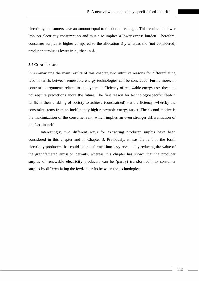
5. A new view on technology-specific feed-in tariffs
112
electricity, consumers save an amount equal to the dotted rectangle. This results in a lower
levy on electricity consumption and thus also implies a lower excess burden. Therefore,
consumer surplus is higher compared to the allocation 𝐴1, whereas the (not considered)
producer surplus is lower in 𝐴2 than in 𝐴1.
5.7 CONCLUSIONS
In summarizing the main results of this chapter, two intuitive reasons for differentiating
feed-in tariffs between renewable energy technologies can be concluded. Furthermore, in
contrast to arguments related to the dynamic efficiency of renewable energy use, these do
not require predictions about the future. The first reason for technology-specific feed-in
tariffs is their enabling of society to achieve (constrained) static efficiency, whereby the
constraint stems from an inefficiently high renewable energy target. The second motive is
the maximization of the consumer rent, which implies an even stronger differentiation of
the feed-in tariffs.
Interestingly, two different ways for extracting producer surplus have been
considered in this chapter and in Chapter 3. Previously, it was the rent of the fossil
electricity producers that could be transformed into levy revenue by reducing the value of
the grandfathered emission permits, whereas this chapter has shown that the producer
surplus of renewable electricity producers can be (partly) transformed into consumer
surplus by differentiating the feed-in tariffs between the technologies.

113
6. Excessive nuclear risk-taking and the need of public policy
6.1 PLAN OF THE CHAPTER12
Topics thus far in this dissertation have focused on the use of renewable energy. However,
another topic in the field of energy economics has recently attracted significant attention:
nuclear energy. Due to the nuclear catastrophe in Japan in 2011, public awareness of the
possibility of severe nuclear accidents has increased, and major political decisions have
been taken. As briefly summarized in Chapter 1, Germany has decided to phase-out
nuclear power even before the operating lifetimes of the existing nuclear power plants will
be achieved. Despite the potential to write much about the process towards this decision
and its impact on Germany’s electricity supply, the aim of this chapter is not to question it.
Moreover, it also does not aim to generally argue in favour or against the use of nuclear
power, but rather intends to apply a perspective in line Musgrave’s understanding of the
role of public policy.
The purpose of this chapter is to outline and discuss one main economic problem
concerning the use of nuclear power in an unbiased way, namely the safety of nuclear
power reactors. It will be explained that owing to a market failure, the safety chosen by the
nuclear power companies might be inefficiently low. Knowing that a market failure
generally implies an inefficient allocation of resources, there are two channels by which
the inefficiency can occur in such a case. Firstly, society might face an inefficiently high
probability of a severe nuclear accident due to the insufficient level of safety. Secondly, if
society is aware of the inefficiently high risk and thus chooses to phase-out nuclear power,
it also misses the optimal allocation, whenever it would have been optimal to continue
using nuclear power with the correctly selected safety level.
Therefore, this chapter provides guidance on what kind of public policy would be
needed to ensure an efficient use of nuclear power, whereby society may still choose not to
use nuclear power once an efficient safety level is achieved, for different reasons. After
providing an introduction to the current state of nuclear energy use around the world, it
will be derived that a negative externality arises and risk-taking of nuclear power
companies (NPCs) is too excessive, both because of the existence of limited liability.
12 The sections 6.3-6.8 are based on joint work with Jakob Eberl, cf. Eberl and Jus (2012).

6. Excessive nuclear risk-taking and the need of public policy
114
Reviewing the current regulation and discussing possible regulatory instruments regarding
their ability to deal with this problem, it will be concluded that neither current regulation
nor those regulatory instruments in their pure form would be able to induce an efficient
risk choice. Therefore, a new regulatory proposal will be presented and discussed in the
final part.
6.2 NUCLEAR ENERGY USE AROUND THE WORLD
The commercial use of nuclear energy to generate electricity began in the 1950s, but only
became an important component in the world’s energy supply at the end of the 1960s. Of
the two possibilities for exploiting nuclear energy, nuclear fission and nuclear fusion, only
nuclear fission has been used commercially to date. Similar to fossil fuel power plants,
nuclear fission reactors also typically generate electricity by heating water and using the
steam to drive turbines. However, the source of the heat does not stem from the burning of
a substance, rather from a (controlled) chain reaction in which atoms are split.
Figure 6.1: Nuclear electricity generation since 1965, by region
Source: BP Statistical Review of World Energy June 2012.
Figures 6.1 and 6.2 illustrate the development of nuclear electricity generation since 1965.
The two major countries in terms of nuclear electricity generation are the United States and
0300600900
1200150018002100240027003000
World
OECD countries
non-OECD countries
Three Mile Island
Chernobyl
Fukushima
United States
TWh

6. Excessive nuclear risk-taking and the need of public policy
115
France, accounting for almost 50 percent of the world’s nuclear electricity generation in
2011.
Nuclear electricity has been losing relative importance in worldwide terms since
the mid-1990s. Whereas it accounted for more than 17 percent of the world’s electricity
generation during the mid-1990s, its share declined to 13 percent in 2010 and only 12
percent in 2011. The reason for this relative decline can be found in its stagnation in the
OECD countries, particularly Germany and Japan, whereas nuclear electricity generation is
rapidly increasing in China and India, for example. The absolute decline in 2011 compared
to 2010 is largely due to a strong decline in Germany (minus 32.6 TWh) and even more so
in Japan (minus 129.5 TWh). Excluding those two countries, the rest of the world’s nuclear
electricity generation even increased by 42.6 TWh in 2011, relative to 2010.
Figure 6.2: Nuclear electricity generation since 1965, by country
Source: BP Statistical Review of World Energy June 2012.
After the terrifying catastrophe in Japan in March 2011, a fundamental reassessment of
nuclear risk generally occurred all around the world. As previously discussed, a complete
phase-out was decided within a few months in Germany, according to which some nuclear
power plants are supposed to be shut down even before their scheduled operational
lifetime. Switzerland has also stated its ambition to phase-out the use of nuclear power,
however only after the operational lifetime is achieved. Belgium, which had already set out
0
60
120
180
240
300
360
420
480France
Japan
South Korea
Three Mile Island
Chernobyl
Fukushima
Germany
China
Russian Fed.
TWh

6. Excessive nuclear risk-taking and the need of public policy
116
and later abandoned a phase-out plan before the Fukushima catastrophe, is now aiming
again to phase-out nuclear power by 2025. However, in the same course, the operation
license for the Tihange 1 nuclear power reactor has been extended until 2025, having been
originally supposed to end in 2015. In Japan, where all reactors were temporarily shut
down for safety revisions, the Ōi nuclear power plant has been reconnected since July
2012. The “Energy & Environment Council” established by the Japanese cabinet office in
July 2011 has recommended not building new nuclear power plants, whereas those existing
are to be restarted once their safety has been assessed (see EEC, 2012).
Figure 6.3: Currently operating nuclear power reactors (upper map), nuclear power reactors currently under construction (lower map)
Source: World Nuclear Association Reactor Database, available at: http://world-nuclear.org/ NuclearDatabase.

6. Excessive nuclear risk-taking and the need of public policy
117
Most other nuclear power using countries have chosen to continue with their nuclear power
plans for the time being, in the same vein as before the Fukushima accident. Moreover,
many countries around the world are even currently expanding their civilian nuclear
programs. The notion that nuclear fission will remain an important source of energy in the
future is also found within the content of the Energy Roadmap 2050, published by the
European Commission in December 2011. It emphasizes the current and future role of
nuclear energy as an ‘important part of Europe’s power generation mix’ considering it
‘needed to provide a significant contribution in the energy transformation process’ (see
EC, 2011b).
As of December 2012, 437 nuclear reactors are operating worldwide, and another
64 are under construction. The list of countries with the most nuclear power reactors under
construction is headed by China (27 reactors under construction), Russia (10) and India
(7), but reactors are currently being built also in the European Union (France, Finland and
Slovakia). The location of these reactors is illustrated in the lower map in Figure 6.3,
whereas the upper map highlights all nuclear reactors in current operation. Moreover, there
a large number of nuclear reactors planned or proposed all around the world. Thus, despite
a general reassessment of nuclear risk after the Fukushima catastrophe, nuclear power is
likely to remain (or become) a significant determinant of many countries’ electricity
supply.
6.3 THE TWO MAJOR PROBLEMS ASSOCIATED WITH THE USE OF NUCLEAR ENERGY
There are two major concerns regarding the use of nuclear fission for the generation of
electricity: nuclear waste and the possibility of (severe) accidents, with both potentially
leading to negative externalities if public policy does not implement proper regulation.
The handling of waste and the pollution of the environment are classical examples
of negative externalities. Nuclear electricity producers would likely choose cheaper ways
for dealing with nuclear waste if regulation did not demand certain rules to be respected.
These cheaper ways would possibly imply higher costs for current society and/or future
generations, which would not be taken into account in their full extent by today’s profit
maximizing NPCs. Therefore, the setting and enforcement of regulation is necessary for an

6. Excessive nuclear risk-taking and the need of public policy
118
efficient allocation to be achieved. Bearing this issue in mind, this chapter places a focus
on the second problem, namely the issue of nuclear catastrophes.
Three terrifying events have occurred in the history of civilian nuclear energy use:
the Three Mile Island accident in 1979, the Chernobyl disaster in 1986, and the Fukushima
Dai-ichi catastrophe in 2011. Given the large number of nuclear reactors worldwide, the
general probability of a severe accident occurring at a nuclear power reactor in a given
year is microscopically small, yet, as the aforementioned catastrophes have proven, such
risk does exist. There is currently no existing alternative that could generate sufficient
amounts of electricity at low costs and without creating some sort of risk. The use of fossil
energy causes climate change and also deaths in the mining and extraction industry,
whereas the generation of renewable electricity is costly as such and suffers from the
problem that electricity cannot yet be stored at reasonable costs. Therefore, the role of
public policy should be to ensure that benefits and costs are fully taken into account by
market participants, who would accordingly find efficient solutions for how to generate
electricity.
With clean-up costs alone that could exceed JPY 20 trillion over the next ten years
(cf. JCER, 2011), the Fukushima accident has reminded the world how strongly a society
can be affected by the use of nuclear energy. At the same, it may be asked whether the
NPCs actively influencing the probability of such an accident occurring are also those who
bear the full costs in the unlikely yet existing case that it occurs. For example, Tokyo
Electric Power Company (TEPCO) reported equity capital to the amount of JPY 2.47
trillion for March 2010, the last annual report published before the 2011 catastrophe (see
TEPCO, 2011). This does not appear small at first glance; however, this amount only
constitutes a small proportion of the actual costs of the Fukushima catastrophe, the
remainder of which cannot be borne by TEPCO. Similarly, the liability of other NPCs
around the world is limited de jure or de facto (by the equity capital of the company); see
Table 6.1 for a brief overview.
This chapter argues that a main problem arises due to the existence of de facto or de
jure limited liability of NPCs. The basic mechanism implies that an NPC cannot lose more
than the legally defined liability capital, or in the worst case its equity capital, regardless of

6. Excessive nuclear risk-taking and the need of public policy
119
the higher damage of a nuclear accident. This reduces the incentive to invest in costly
nuclear safety, thus leading to an inefficient safety level in nuclear reactors.
Table 6.1: De facto vs. de jure limited liability, selected countries and selected NPCs
Selection of countries with de jure
limited liabilitya Countries with de facto limited liabilityb
China RMB 300 million
Germany
E.ON EUR 39.6 billion Czech Republic CZK 8 billion RWE EUR 9.9 billion
France EUR 91 million EnBW EUR 6.1 billion
India INR 5 billion Vattenfall SEK 138.9
United Kingdom GBP 140 million Japan TEPCO JPY 2.47c trillion
United States USD 375 million Switzerland Axpo CHF 7.6 billion a right column: de jure national liability limitation; b right column: NPCs’ equity capital in 2011; c as of March 2010; Source: Eberl and Jus (2012).
The de jure limitations of nuclear liability have already existed for a long time, as will be
emphasized in section 6.5. A major goal of nuclear liability regulation has been to protect
NPCs against potentially ruinous claims. By introducing a limit up to which they can be
made liable, liability is passed from the operator to a third party for any damage beyond
this limit. In essence, this limitation has been justified by the social benefits of nuclear
power, creating a tacit acceptance of nuclear risk by the society. At the same time, it has
also increased the profitability of the nuclear industry, thereby fostering its development.
The downside of this will be explained in the following section, which will outline the
underlying theory and illustrate why the existence of limited liability leads to excessive
risk-taking.
6.4 LIMITED LIABILITY AND EXCESSIVE NUCLEAR RISK-TAKING
Suppose a NPC maximizes its profit by choosing its nuclear power reactor’s level of risk.
It can build and operate a reactor with lower safety, thus reducing its costs (thereby
increasing its profits), however this also leads to a higher probability of a catastrophic
accident occurring. The maximization problem is:

6. Excessive nuclear risk-taking and the need of public policy
120
max𝑅
�1 − 𝑝(𝑅)� ∙ �𝐸 + Π(𝑅)� + 𝑝(𝑅) ∙ 𝑚𝑎𝑥(𝐸 − 𝐿, 0) − 𝐸 (6.1)
where 𝑅 is the level of risk chosen and 𝑝(𝑅), with 𝑝′(𝑅) > 0, is the probability of a
catastrophic accident. Only a two-point distribution is considered for the sake of simplicity,
meaning that if an accident occurs then the loss of the NPC is 𝐿. The variable Π denotes
the profits of the NPC in the case that no accident occurs, and it is increasing in 𝑅 as a
lower level of safety is less costly providing no accident takes place. Finally, 𝐸 is the
equity capital of the NPC, which by the nature of a firm with limited liability, can at most
be lost in case of an accident. Thus, in the case of no catastrophe the equity of the NPC
remains within the firm, while additionally profits are generated. In the other state of the
world, the wealth of the NPC is reduced to 𝐸 − 𝐿 or zero, whichever of the two is larger.
Hence, there are two possible outcomes when a catastrophic accident occurs: the
liable equity capital can be sufficient to cover the losses, or it can be lower than the
resulting damage. Denoting by 𝐿0 a possible damage for which holds that 𝐸 ≥ 𝐿0, the
maximization problem of the NPC becomes
max𝑅
�1 − 𝑝(𝑅)� ∙ �𝐸 + Π(𝑅)� + 𝑝(𝑅) ∙ (𝐸 − 𝐿0) − 𝐸 (6.2)
and the first order condition is:
�1 − 𝑝(𝑅∗)� ∙ Π′(𝑅∗) − 𝑝′(𝑅∗) ∙ (Π(𝑅∗) + 𝐿0) = 0
↔ �1 − 𝑝(𝑅∗)� ∙ Π′(𝑅∗)�������������benefit of a marginal
increase in risk
= 𝑝′(𝑅∗) ∙ (Π(𝑅∗) + 𝐸) + 𝑝′(𝑅∗) ∙ (𝐿0 − 𝐸)���������������������������cost of a marginal
increase in risk
(6.3)
Since all costs and benefits are fully taken into account by the NPS, the resulting risk
choice 𝑅∗ satisfies allocative efficiency (in the absence of other market failures), and can
thus be regarded as the benchmark in the following.
In contrast to this case, suppose that the damage from a nuclear accident, now
denoted by 𝐿1, would exceed the equity capital of the NPC, that is, 𝐸 < 𝐿1. This is a
realistic assumption as shown in the example of the Fukushima catastrophe. Since the NPC
is a firm with limited liability, the maximization problem becomes
max𝑅
�1 − 𝑝(𝑅)� ∙ �𝐸 + Π(𝑅)� − 𝐸 (6.4)
and the first order condition is:

6. Excessive nuclear risk-taking and the need of public policy
121
�1 − 𝑝(𝑅∗∗)� ∙ Π′(𝑅∗∗) − 𝑝′(𝑅∗∗) ∙ �𝐸 + Π(𝑅∗∗)� = 0
↔ �1 − 𝑝(𝑅∗∗)� ∙ Π′(𝑅∗∗)���������������benefit of a marginal
increase in risk
= 𝑝′(𝑅∗∗) ∙ (Π(𝑅∗∗) + 𝐸)���������������cost of a marginal
increase in risk under binding limited liability
(6.5)
where 𝑅∗∗ is the risk-taking of the NPC under the assumptions made. The difference
between this case and the previously derived efficient risk-taking is that under binding
limited liability the term 𝑝′(𝑅) ∙ (𝐿 − 𝐸) no longer appears. The NPC can at most be made
liable with the equity capital 𝐸, and thus does not consider any cost beyond 𝐸. According
to Shavell (1986), in this case the NPC is ‘judgment proof’.
Figure 6.4: The effect of limited liability on the NPC’s risk preference
Source: cf. Sinn (1983) and Eberl and Jus (2012).
Figure 6.4 illustrates the underlying reasoning, whereby the change in the legal wealth of
the NPC is shown on the horizontal axis, whereas the change in the actual wealth is on the
vertical axis. The actual wealth can at most decline by 𝐸, whereas the legal wealth in the
case of a severe accident with high damage can decrease by 𝐿1. Thus, due to limited
liability, the NPC’s change in the actual profit is horizontal for any loss that is larger than
its equity capital. It can be seen from Figure 6.4 that if the equity capital is sufficient to pay
∆ legal wealth Π(𝑅∗∗)
−𝐿1
−𝐸
∆ actual wealth, 𝐴𝐴
45° 𝐸[𝐴𝐴] 𝐶𝐸
no accident
catastrophic accident

6. Excessive nuclear risk-taking and the need of public policy
122
for the damage, the expected change in the legal wealth and the actual wealth coincide.
However, if the potential loss exceeds the equity capital, the expected actual wealth is
higher than the expected legal wealth. In such a case, an otherwise risk-neutral NPC
strictly prefers the gamble between the two possible outcomes, which gives an expected
change in the actual wealth of 𝐸[𝐴𝐴], over a certain change in the legal wealth of the same
amount. In fact, to be indifferent it would require a certain change in the legal wealth of
𝐶𝐸, which is its certainty equivalent. Thus, given that the NPC operates under limited
liability and potential losses can exceed its equity capital, an artificial risk-preference
occurs. In terms of reactor safety, this means that the NPC chooses an inefficiently low
level of care, as can also be seen from condition (6.5) in comparison with (6.3).
As explained in Sinn (1980, 1982. 1983), the underlying reason for the extensive
risk preference is that the function describing the change in the actual wealth becomes de
facto convex, indicating a risk-loving behaviour that can be interpreted as a preference of
the NPC for choosing an inefficiently low safety. This argument is also discussed by Tyran
and Zweifel (1993), Strand (1994) and Trebilcock and Winter (1997), with a review of
other related literature provided by van’t Veld and Hutchinson (2009).
6.5 LIABILITY REGULATION OF THE NUCLEAR POWER INDUSTRY AROUND THE WORLD
The development of nuclear power liability regulation and its current state are briefly
summarized in the following section, referring to Faure and Vanden Borre (2008) for an
extensive analysis of international nuclear liability.
Passed in the United States in 1957, the Price-Anderson Act (cf. US NRC, 2012)
was the first comprehensive nuclear liability law and has been central to the issue of
liability in nuclear accidents. It has been repeatedly renewed (with amendments), most
recently in 2005 for another 20 years, with the defined amount of an NPC’s liability
gradually increasing over time. Today, coverage in the case of accident is provided by the
nuclear industry itself on a two-tier basis. At the first layer, all NPCs are strictly and
individually liable, required to purchase USD 375 million of liability coverage per reactor,
provided by a private insurance pool. At the second layer, coverage is supplied by a mutual
and solidary risk-sharing agreement among the NPCs. This risk-sharing pool is funded
through retrospective payments in the case of a nuclear accident, which can reach up to

6. Excessive nuclear risk-taking and the need of public policy
123
USD 112 million per reactor. In total, this two-tier system provides an aggregate sum of
USD 12 billion of liability capital.
Liability regulation of the nuclear industry outside the United States is based on
two conventions, the Paris Convention (NEA, 1960) and the Vienna Convention (IAEA,
1963), and on individual countries’ national regulations. Whereas the Paris Convention
covers European states, those from all over the world are party to the Vienna Convention.
The national regulation in most countries that fall under one of these two conventions
usually follow the proposed liability framework, with only few exceptions where the
liability of NPCs is considerably higher than that demanded by the conventions.
The basic characteristics of the Paris Convention can be summarised as follows: (1)
nuclear companies are strictly liable for any third-party damage, thus their liability is
irrespective of their own fault;13 (2) liability is fully channelled to the NPCs, thus only they
can be sued; and (3) liability is limited to a pre-defined amount and a specified period of
time within which claims can be made. More specifically, liability was originally supposed
to be limited to a maximum SDR 15 million, whereas the minimum was supposed to be
SDR 5 million;14 however, national legislation has been allowed to provide for a higher,
but necessarily limited, amount. Finally, (4) the liability has to be covered by mandatory
insurance or some other financial security, to be held by the NPCs. The Paris Convention
was amended in 1964, 1982 and in 2004, and according to the most recent amendment the
minimum liability of nuclear operators is supposed to be raised to 700 million (cf. NEA,
2004, Art. 7). Moreover, the sentence excluding any liability for damage owing to ‘a grave
natural disaster of an exceptional character’ has been removed (cf. NEA, 1960, and NEA,
2004). It was also the first amendment to allow the participation of countries with a de jure
unlimited liability in place (Germany and Switzerland), thereby implicitly agreeing to this
type of national liability legislation. However, the 2004 amendment is not yet in force as
only Switzerland and Norway have ratified it to date.
In 1963, the Brussels Convention, supplementing the Paris Convention, introduced
that in addition to the NPC, the state in which the nuclear accident occurs is also liable,
13 Cf. Shavell (1980, 1982) for a comprehensive analysis of the incentives strict liability and negligence rules have on risk-taking. 14 A Special Drawing Right (SDR) is a unit defined by the International Monetary Fund (IMF). As of March 2012, the value of one SDR equals USD 0.66, EUR 0.423, JPY 12.1, and GBP 0.111.

6. Excessive nuclear risk-taking and the need of public policy
124
with a limit set at SDR 70 million. Moreover, all signatory states agreed to be jointly liable
for claims, whereby each state is obliged to supply up to SDR 50 million.
Parallel to the Paris and Brussels conventions, the IAEA’s 1963 Vienna Convention
introduced a regulatory framework signed by 38 countries, including the Russian
Federation, Ukraine, and Czech Republic, but also a large number of countries that do not
even have a civilian nuclear program. It shares the basic principles of the Paris Convention,
with the minimum liability of the NPCs initially only supposed to be USD 5 million. It was
amended once in 1997, with the main difference being a seemingly higher minimum
liability limit of NPCs in the amount at least of SDR 300 million. However, this may be
reduced to SDR 150 million or only SDR 5 million, whereby the lower amounts are
allowed if public funds are provided to cover the sum of SDR 300 million (cf. IAEA, 1997,
Art. 7).
Following the 1986 nuclear accident at Chernobyl, efforts to clarify the
applicability of the two ‘competing’ conventions have led to the establishment of a Joint
Protocol, according to which only one of the two conventions shall apply to a nuclear
accident, namely the one to which the country within whose territory the nuclear reactor is
situated is party to (cf. NEA and IAEA, 1988).
The heterogeneity in national regulation stems from a few countries having
substantially stricter rules than demanded by the conventions. For example, liability
legislation in Germany far exceeds the requirements of the (amended) Paris Convention.
Together with Japan and Switzerland, Germany is one of only three countries with a
legally unlimited liability of NPCs. In order to ensure a desired minimum amount of
financial security, it requires the amount of EUR 2.5 billion per reactor to be guaranteed by
both a nuclear insurance pool and risk-sharing agreement between the NPCs. In addition to
financial security, the European Union provides EUR 300 million in accordance with the
Brussels Convention in case of an accident. For any loss exceeding the aggregate amount,
the NPCs’ liability is legally unlimited; however, this definition of unlimited liability only
constitutes a legal property that cannot actually be sustained. In Switzerland, where NPCs
are also de jure unlimitedly liable, they are required to hold financial security to the
amount of CHF 1 billion. By contrast, the liability regulation of NPCs in France is weaker,

6. Excessive nuclear risk-taking and the need of public policy
125
with the liability of the state-owned NPC15 being de jure limited to an amount of EUR 91
million (projected to increase to EUR 700 million, according to the 2004 amendment),
which must be insured. This is also the case in the Czech Republic, where the de jure
liability limit of CZK 8 billion necessitates insurance.
As they are not party to any international conventions and thus rely on their own
arrangements, China, India and Japan occupy a special position in global nuclear liability
legislation. China passed an interim law on nuclear liability in 1986, containing the basic
properties of the international conventions. NPCs’ liability limit was increased to RMB
300 million in 2007, above which the state is legally liable for up to RMB 800 million.
However, this legal regime is under revision, with China aiming to modify its nuclear
energy law along with its nuclear expansion (see WNA, 2012a). In 2010, the Indian
government passed the so-called Nuclear Liability Act, which brings its liability regulation
broadly in line with international conventions. The act renders NPCs liable for nuclear
accidents up to an amount of INR 5 billion (although not exclusively).
NPCs’ liability is strict, exclusive, and legally unlimited in Japan, and furthermore
a financial security must be provided to the amount of JPY 120 billion. In addition, Japan’s
1961 Act on Compensation for Nuclear Damage (cf. NSC of Japan, 1961) allows for an
NPC to be relieved of liability in claims resulting from ‘a grave natural disaster of an
exceptional character’, the relevance of which came into discussion after the Fukushima
catastrophe. Regardless of this paragraph, the catastrophe has provided evidence that the
costs of a large-scale nuclear accident can easily exceed the means of an NPC, and that
society must eventually step in. Within this context, the Japanese government decided to
provide financial assistance for compensation payments and clean-up costs, demanding an
annual fee from TEPCO accordingly. The main reason for bailing TEPCO out was its
essential role in maintaining adequate power supply and the need to ensure the safety of its
other power plants. According to government estimates, TEPCO will be able to complete
its repayments in 10 to 13 years, after which it is supposed to revert to being a fully private
company with no government involvement (cf. WNA, 2012b).
The main insight gleaned from studying nuclear liability regulation around the
world is that the liability for losses from catastrophic accidents is either de facto limited by 15 As of August 2012, the French state holds 84.8 percent of the shares of Électricité de France (EdF), the owner of all French nuclear power plants.

6. Excessive nuclear risk-taking and the need of public policy
126
the NPCs’ equity capital (as in Germany, Switzerland and Japan) or de jure limited by
national legislation (all other countries). Thus, some countries have chosen to limit NPCs’
liability explicitly while firms in other countries are liable, at most, with their equity capital
by their nature. As previously discussed, the consequences of limited liability become
relevant in both cases. On this basis, the following section critically discusses the
regulatory instruments that could be applied by a regulatory authority.
6.6 POLICY INSTRUMENTS WITH THE AIM OF ATTAINING THE OPTIMAL LEVEL OF SAFETY
Two schools of thought developed in the twentieth century could be applied in order to
overcome the problem stemming from the existence of a negative externality, as described
here. The first, the Coasian solution (drawing from Coase, 1960), would argue that
defining property rights and letting the involved parties negotiate potential outcomes can
solve the problem at hand. The other, the Pigouvian approach, calls for (stronger)
government intervention through setting a price on the activity generating the externality
(Pigou, 1920).
Applying the former framework to the nuclear industry, one could interpret a
laissez-faire situation as a case in which the property rights for any potential damage are
given to the NPC. In such a case, the NPC could choose any level of risk without being
liable for the consequences. The defining of a liability limit is similar, with the only
difference in property rights for a (small) share of the damage being given to the injured
party. In line with Coase (1960), one could argue that negotiations between potential
victims and the NPC could result in a Pareto-optimal level of risk-taking. However, this
type of negotiation is hardly practicable since nuclear risk is dispersed over vastly many
individuals, and moreover any attempt to specify private contracts over an efficient risk
level would suffer from the public good problem (see, Sinn, 1983), in addition to other
fundamental barriers such as incomplete information. Therefore, society is unable to obtain
a contractual relationship with the NPC, and the NPC could thus not be forced to pay for a
potential damage ex ante, whereas ex post liability is limited.
Therefore, Coasian irrelevance does not apply, and the risk allocation can be
improved only if the government implements measures in representing the interest of
society that increase the liability of the NPC or Pigouvian type of price mechanism on the

6. Excessive nuclear risk-taking and the need of public policy
127
activity that causes the externality, or both. Existing literature on the regulation of risk-
taking in the nuclear power industry discusses several instruments that could be applied,
which are reviewed and evaluated in the following sections, in terms of their ability to
reduce the nuclear power company’s incentives to take excessive risks.
SAFETY REGULATION
Recognizing that nuclear reactors are generally not sufficiently safe in theory, several
papers propose the setting of safety standards or its joint use with other instruments (see,
for example, Shavell, 1984, Kolstad et al., 1990, Schmitz, 2000). The setting of safety
standards attempts to improve (or optimize) the level of precaution by defining a large set
of measures to be implemented or followed by NPCs.
A repeated criticism of command-and-control measures set by a (central) regulatory
authority is that this authority might only possess imperfect information and would
therefore be unable to properly define safety regulation (see, for example, Baumol and
Oates, 1971; Shavell, 1984). This may hold particularly strongly for the regulation of
nuclear power, which by its nature requires an understanding of very complex processes.
Trebilcock and Winter (1997) discuss the implications of this type of complexity for
regulation, whereas Bredimas and Nuttall (2008) comprehensively analyse this issue in the
context of several countries. Faure and Skogh (1992) also highlight that obtaining
necessary information is difficult for a regulator, who thus might eventually depend on
information provided by the nuclear industry itself. However, since the industry acts in its
own interest, it is likely to provide inaccurate signals; in which case regulation may
consequently become too lax in some respects and too strict in others.
In a very general sense, it is unclear whether a regulator is better able to achieve the
proper level of care by setting safety standards, or alternatively whether (more) market-
based instruments, proposed and discussed here later, are more effective. However, there
are various other reasons why the efficient level of care cannot be implemented by safety
regulation alone.
One such reason is that enforcement is not (or only incompletely) guaranteed, even
when safety regulation is defined by law; see Downing and Watson (1974) for the first
enforcement model in the context of environmental policy, and for related work,

6. Excessive nuclear risk-taking and the need of public policy
128
Harrington (1988), Kambhu (1989), and Wang et al. (2003). A second reason is that
nuclear power plants are unequal and thus uniform safety regulation cannot perfectly
internalize the externality; it may be too strict for some reactors or processes and too lax
for others. Thirdly, as safety regulation also concerns the continual monitoring and
reassessment of precautionary measures, it would need to closely follow technological
progress to recognize potentially harmful developments and demand the quick
implementation of new standards. However, given that even the ratification of the
international conventions has taken many years (often five or more), it is doubtful whether
a regulator is able to achieve this sufficiently well. Fourthly, regulatory competition
between states may arise, resulting in inefficiently low safety standards. If a country
demanded higher standards, the NPC might decide to build the reactor in a neighbouring
country, which would harm the country with strict standards in several ways. This type of
‘regulatory race to the bottom’ was discussed in similar contexts by Wilson (1996), Wilson
(1999), and Oates (2002).
Fifthly, complementing the initial argument in this subsection, the regulator might
not have the incentive or ability to be sufficiently informed to elaborate a comprehensive
and appropriate regulatory framework. Whereas Poterba and Rueben (1994) investigate
wage differentials between public and private sector employees, in line with this Borjas
(2003) finds that the public sector is unable to attract the labor force’s most qualified
individuals as it cannot compete with the private sector in wage terms. Finally, command-
and-control measures are often accused of creating enormous inefficiencies. Taken to the
extreme, scholars such as Coase (1960) have argued that direct regulation might not
necessarily provide better results than leaving the problem to the market.
While often neglecting the problems discussed in the previous paragraph, safety
and liability regulation are sometimes viewed as substitutes for correcting externalities.
Consequently, the policy recommendation has involved choosing the instrument that
causes the least administrative cost for achieving a given goal (for early discussions of
related issues see, for example, Calabresi, 1970, and Wittman, 1977). However, in practice
we observe that both instruments are often jointly used as in nuclear power regulation, for
instance. Developing this observation, Shavell (1984), Kolstad et al. (1990) and Schmitz
(2000) find that safety regulation and liability rules may be complementary as their joint

6. Excessive nuclear risk-taking and the need of public policy
129
use can correct the inefficiencies of using either of the two alone. Shavell (1984) argues
that it is better to use both safety and liability regulation under asymmetric information and
enforcement problems, where the regulatory standard can be set lower than if only safety
regulation was used. Kolstad et al. (1990) and Schmitz (2000) argue similarly, whereby the
former paper bases its reasoning on an imperfection in the definition of legal standards and
the latter finds that wealth differences between firms do not change this result.
In line with these arguments, safety regulation is considered an important means of
complementing liability regulation, particularly by defining a minimum level of
precaution. If enforced, the setting of safety standards would guarantee a lower bound on
the precautionary measures of an NPC, providing a basis for the application of other
instruments. This potential advantage of safety regulation is further elaborated as follows,
explaining under which conditions safety regulation would be neutral, beneficial or even
harmful as a complement to the proposed new regulation.
MINIMUM EQUITY CAPITAL REQUIREMENTS
Defining minimum equity requirements (in equity-to-assets ratio terms) is a commonly
used instrument to regulate the problem of limited liability in the banking sector (cf. Sinn,
2003). Despite the causes and consequences in the banking sector appearing to be very
similar, there is one crucial difference in the nuclear industry: whereas a bank’s maximum
third-party loss is at maximum defined by the bank’s liabilities (stated in the balance
sheet), even under the assumption of perfectly correlated risks, the potentially catastrophic
damages of a large-scale nuclear accident are not represented on an NPC’s balance sheet.
Therefore, even the requirement to finance all assets with 100 percent liable equity capital
would not fully internalise excessive nuclear risk-taking (providing there are fewer assets
than a potential catastrophic damage). However, this would lower the extent of the
negative externality, given that the NPCs’ de facto liability capital would increase.
MANDATORY INSURANCE
Among others, Trebilcock and Winter (1997) suggest mandatory liability insurance for
reducing the incentives of excessive risk-taking. This proposal has been followed by
several countries, where NPCs are required to cover a specified amount with insurance.

6. Excessive nuclear risk-taking and the need of public policy
130
However, these amounts are tiny compared with the potential damage of a catastrophe, and
thus the effectiveness is very limited in terms of setting incentives for improving safety. A
more effective alternative would involve requiring the entire potential nuclear damage to
be insured, thereby transferring the full risk from the NPC to a third party. It could be
argued that this would induce an efficient outcome, as the NPC would have to pay a
premium at least equal to the expected loss. Consequently, the insurer would punish the
NPC for excessive risk-taking, which would become costly, and the negative externality
would subsequently vanish.
However, imposing a full mandatory insurance for potential nuclear accidents
entails several shortcomings. First of all, the insurability of catastrophic events –
characterized by a low occurrence frequency, yet highly severe impacts – has generally
been questioned within existing literature.16 As a prime example, nuclear risk has been
repeatedly regarded as non-actuarial (see, for example, Litzenberger et al., 1996;
Kunreuther, 1997; Cutler and Zeckhauser, 1999; Radetzki and Radetzki, 2000).
However, the most important reason why mandatory insurance might not be a
reasonable alternative is that the capital resources available to the insurance industry may
also be insufficient to cover the damages of nuclear catastrophes. As insurance companies
are similarly judgment-proof, they might not have the incentive to calculate and charge
actuarially correct premiums (even if this were possible), but would also maximise their
profits taking their own limited liability into account. In such a case, the insurance
premiums charged upon the nuclear industry would not reflect the true expected loss, and
consequently the effect of limited liability on risk-taking would only be shifted from one
industry to another without solving the core problem.17
MUTUAL RISK-SHARING POOLS
In contrast to risk being transferred to a third party in the case of insurance, the risk in a
mutual risk-sharing pool is shared among the risk-creating parties. Therefore, the NPCs
agree on an ex post sharing of the costs of a catastrophic accident. Whereas insurance
presumes an ex ante pricing of nuclear risk, mutual risk-sharing offers the particular 16 This is the case for both natural and man-made catastrophes, to different extents. See, among others, Kunreuther (1997) and Cutler and Zeckhauser (1999). 17 See Buck and Jus, 2009, for a similar argument concerning the possibility of securitization in the banking industry, which opens a channel for circumventing the introduction of stricter equity requirements on one layer of banking.

6. Excessive nuclear risk-taking and the need of public policy
131
advantage that only paying the actual costs eliminates the need to estimate potential
damages and probabilities in advance. Such advantages of mutual risk-sharing over
insurance have been extensively discussed and emphasised by, among others, Skogh
(1999), Faure (2004), Faure and Fiore (2008), and Skogh (2008), who elaborates on the
theoretical foundation of mutual risk-sharing. Skogh (1999) explains why it is advisable
for parties facing similar risks to share them in common pools. Furthermore, Faure (2004)
investigates whether an extended mutual agreement between NPCs could serve as an
alternative to the nuclear power liability regulation currently in place. Faure and Fiore
(2008) discuss possible structures and the potential for a more comprehensive mutual risk-
sharing agreement among Europe’s NPCs.
There are several examples of mutual risk-sharing agreements, for instance in the
United States, the Nuclear Electric Insurance Limited (NEIL) and the Overseas NEIL
(ONEIL), or in Europe, the European Mutual Association for the Nuclear Industry
(EMANI) and the European Liability Insurance for the Nuclear Industry (ELINI). Mutual
risk-sharing generally creates a collective responsibility for risk-taking; moreover making
NPCs liable generates incentives to prevent accidents, which implies a reduction of
excessive risk-taking. However, risk-sharing pools suffer from the fundamental problem of
collective action: the higher the number of NPCs financing the pool, the stronger the
tendency towards free-riding, as individual responsibility shrinks and peer-monitoring
becomes more costly. Furthermore, the effectiveness of this type of regulation diminishes
as an NPC’s share of the pool declines.
CATASTROPHE BONDS
Catastrophe (cat) bonds represent one means of spreading the risk of potentially large
losses via financial instruments (namely via capital markets). A cat bond offers investors a
return above the risk-free rate when a specified catastrophic event does not occur, but
otherwise requires the sacrifice of interest or principal. The general idea of cat bonds is
explained by Cummins and Weiss (2009), who also provide an overview of related
literature.18 Thus far, cat bonds have generally been employed by insurers as an alternative
to traditional re-insurance, and by re-insurers usually in atomising the risk of natural 18 For analyses of other private and alternative, arrangements for transferring risk, see Wagner, 1998; Radetzki and Radetzki, 2000.

6. Excessive nuclear risk-taking and the need of public policy
132
catastrophes such as earthquakes or hurricanes (see Evans, 2011; for a comparison between
cat bonds and re-insurance, see Gibson et al., 2007; Cummins, 2012). Mexico was the first
sovereign to offer cat bonds, thereby protecting itself against the risk of natural
catastrophes (see, for example, Cardenas et al., 2007; Michel-Kerjanet al., 2011). An
overview of the development and current state of cat bond markets can be found in
Cummins (2012) and Swiss Re (2012). It is evident that issuance volumes declined sharply
in 2008 owing to the financial crisis, and have still not fully recovered. In 2011, they
reached a volume of USD 5 billion.
Besides natural catastrophes, the idea of also employing cat bonds for nuclear
accidents was discussed by Tyran and Zweifel (1993), offering a description of how to
internalise environmental risks such as potential nuclear catastrophes via capital markets.
They observe that NPCs could emit cat bonds, through which nuclear risk is spread among
a large number of investors. The principal received for each cat bond issued is supposed to
be placed in risk-free assets, for example certain treasury bonds. The spread between the
cat bond interest and the interest on a risk-free bond represents the market assessment of
the risk of a nuclear accident, if this is specified as the trigger for the cat bonds’ default.
Hence, as nuclear risk is priced by capital markets, risk-taking becomes costly for the
NPCs. Consequently, NPCs taking excessive risk may either revise their strategy to reduce
the premiums paid on cat bonds or even leave the market if this business becomes too
costly for them. A further advantage of catastrophe bonds is that risks can be diversified
internationally, thus diluting the strong impact on the economy where the accident occurs.
Tyran and Zweifel (1993) argue that investors would have an incentive to remain well-
informed and would on average estimate the risk correctly.
Leaving aside some well-known problems of cat bonds (such as high transactions
costs), the main issue in the case of nuclear power is that NPCs would not voluntarily emit
cat bonds. Paying a premium on cat bonds would imply additional costs and undermine the
benefits of limited liability, and thus the regulatory authority would have to stipulate their
emission. Despite the global cat bond market currently being relatively small, one could
argue that if the supply of cat bonds was made perfectly inelastic by regulation, it would
only be a matter of the price of the cat bonds for the demand to emerge.

6. Excessive nuclear risk-taking and the need of public policy
133
Figure 6.5: Global stock of equity and debt outstanding in trillion US dollar, end-of-year, constant 2010 exchange rates
Source: Roxburgh et al. (2011)
Concerning the externality from limited liability, a cat bond would achieve full
effectiveness on risk-taking if any potential damage would need to be covered for every
nuclear reactor. To cite an example, given the currently estimated damages of the
Fukushima accident, suppose that the regulatory authority could demand an emission
volume of USD 200 billion per reactor. This would likely outbalance any reasonable scope
of the cat bond market given that there are more than 400 nuclear reactors operating
worldwide, and therefore an amount in excess of USD 80 trillion would need to be
invested in cat bonds. For the purpose of comparison, Figure 6.5 depicts the total global
financial stock, measured as the sum of debt and equity outstanding, which constituted
USD 212 trillion in 2010. Hence, the argument of a correct pricing of risk of even a large
volume of cat bonds is likely to remain of a theoretical nature, given that a constraint on
the properly functioning market size certainly exists in reality. Despite there being a surge
for diversification and nuclear cat bonds offering the favourable property of generally not
being affected by other shocks to the economy, a full coverage for all reactors appears
impossible.
Therefore, although the idea of cat bonds sounds very promising, the nature of their
implementation is highly open to debate. Demanding any smaller amount of cat bond
45 55 65 34 48 54
25 28
30
32 37
41 6 7
8
8
9 10
29 35
41
41
44 42
11
14
15
16
16 15
38
40
43
45
47 49
2005 2006 2007 2008 2009 2010
Stock market capitalization
Public debt securities outstanding
Nonfinancial corporate bonds outstanding
Financial corporate bonds outstanding
Securitized loans outstanding
Nonsecuritized loans outstanding
155
179
202
175
201 212

6. Excessive nuclear risk-taking and the need of public policy
134
emissions than potential damages would re-introduce the negative externality of limited
liability partially. For this reason, the following section offers a proposal that partly relies
on cat bonds and their favourable properties, and also has the potential to largely overcome
the aforementioned market-size problem.
6.7 TAXING NUCLEAR RISK WITH THE HELP OF CAPITAL MARKETS
Having highlighted that current liability regulation might imply severe incentives for
excessive risk-taking and reviewed various regulatory instruments, this section proposes a
new method for the regulation of liability in the nuclear industry. This involves the major
aim of internalising the externality of excessive risk-taking, which could be best
accomplished by combining the strength of private markets with a Pigouvian-type of
public intervention. The proposal demands using the ability of capital markets to evaluate
risk-taking and society’s reserve capacity to absorb high risks in order to achieve the
desired level of nuclear reactor safety.
Figure 6.6: Schematic illustration of the proposed regulation
Source: Eberl and Jus (2012).

6. Excessive nuclear risk-taking and the need of public policy
135
The basic idea can be summarized as a two-stage approach, depicted in Figure 6.6. In the
first stage, by pricing a specified volume of cat bonds, capital markets provide an
assessment of the risk stemming from each nuclear reactor. In the second stage, the
regulatory authority employs this observable risk-assessment and intervenes by charging a
Pigouvian tax equal to an actuarially fair premium, thereby – under ideal conditions –
inducing the socially optimal level of risk-taking. Eventually, society adopts the role of an
explicit insurer for nuclear risk. The main arguments in support of this solution are
outlined below, prior to discussing the details relevant to its implementation.
This analysis has highlighted several issues prompting the conclusion that neither
public safety regulation nor market-based instruments can solve the problem of excessive
nuclear risk-taking in pure form alone. In contrast to Tyran and Zweifel (1993), the
approach described in this section does not aim to establish comprehensive loss coverage
on capital markets, rather it uses cat bond markets only for risk assessment and delegates
any further responsibility to the regulator. Specifically, the proposal demands that NPCs
are obliged to issue cat bonds for each reactor in a volume representing only a fraction of
the potential costs of a large-scale accident. For example, an amount of USD 10 billion per
nuclear reactor could be considered. Despite this seeming large at first glance, even if this
was achieved for the 400-plus reactors worldwide, the total sum would only lead to a
market size of just over USD 4 trillion, or around 30 percent relative to current US public
debt. Given that the recent crises have revealed that investment portfolios were often not
sufficiently diversified, it appears reasonable to assume that there might be sufficient
demand for large amounts of cat bonds. From this perspective, the introduction of a cat
bond model could be timely, since the inclusion of nuclear accident related securities
would increase the portfolio diversification.
However, stipulating a cat bond issuance of some specified amount lower than the
potential damage of a nuclear accident would not fully overcome the problem of excessive
risk-taking, as outlined by previous arguments. However, capital market offers the crucial
advantage of regulators being able to obtain an assessment of the probability of a
catastrophe, given that the cat bond defaults when such an event occurs. Measured against
a risk-free interest rate, the interest premium would exactly reflect the accident probability.

6. Excessive nuclear risk-taking and the need of public policy
136
Alternatively, it could be measured against the safest reactor according to capital markets,
which could represent a good approximation of the risk-free interest rate.
Naturally, there are certain problems to overcome, as discussed below;
nevertheless, such a scheme would offer two particular advantages: (1) overcoming
potential liquidity/capacity problems in capital markets, thus isolating the actual risk from
other capital market imperfections; and (2) the risk assessment is transparent and the risks
of various reactors comparable, as the cat bond issuance is reactor-specific.
It is disputable whether capital markets are able to properly evaluate the risks of
nuclear power. Having failed to price a number of risks correctly in the recent past, it could
be argued capital markets are generally likely to fail. On the contrary, one could, also argue
that future assessment will be more cautious precisely because of these events, possibly
even overestimating certain risks. While neither of them can be proven, it is important to
note that even an incorrect risk-assessment by capital markets does not necessarily lead to
an inefficiently low level of precaution. What matters is the pricing of safety differences
and improvements, rather than the pricing of the level of safety. For instance, if a reactor is
assessed as being relatively safe by capital markets, despite actually being rather unsafe, an
incentive for safety improvements would still be set providing the NPC could sufficiently
improve the conditions under which it can issue cat bonds. Under certain conditions (even
in the case of the risk of nuclear power being under-priced), this may lead to an excessive
level of safety if capital markets reduce the interest premium too generously when the NPC
improves safety.
The correct assessment of safety differences and safety improvements can be
largely reduced to the question of whether investors can obtain information at sufficiently
low costs. If it is too costly for potential cat bond underwriters to acquire information about
differences between reactors or safety changes in a specific reactor, capital markets would
no longer be able to set adequate incentives. Thus, it is vitally important to establish a set
of measures to make this market more efficient. As argued by Tyran and Zweifel (1993),
(private) nuclear rating agencies could emerge, where moral hazard problems as discussed
for existing rating agencies would need to be avoided (see, for instance, Bolton et al., 2012,
Dittrich, 2007, and Pagano and Volpin, 2010). However, it would also be in the self-
interest of the NPCs to provide information (for instance, by issuing reports) about the

6. Excessive nuclear risk-taking and the need of public policy
137
safety of their reactor and be as transparent as possible, since a lack of transparency could
be interpreted as a sign of not being safe by financial markets.
Moreover, two reasons act in favour of believing that capital markets would not
neglect the risks of nuclear accidents: on the one hand, the recent crises have sensitised
investors that even highly improbable events may actually occur; and on the other hand,
the Fukushima catastrophe itself has proven the specific risk of nuclear power. A similar
argument was discussed by Dell’Ariccia et al. (2006), highlighting that the non-bailout of
Russia in August 1998 has increased the cross-country spreads, sensitizing investors that
such risks do exist. Furthermore, Cummins and Weiss (2009) argue that securities markets
are more efficient than insurance markets in reducing information asymmetries and
facilitating price formation.
Having outlined the first stage of the proposal, it is important to explain what the
regulatory authority should do in the second stage. Once again, it shall be emphasised that
a Coasian solution to the problem is not feasible, moreover that the regulator must
intervene in a Pigouvian way if a full liability of NPCs is not implementable. Observing
the reactor-specific interest premium of a cat bond over a risk-free bond, the regulator
defines a tax for each nuclear power reactor to be paid by the NPC. The tax is proportional
to the interest premium, and is thus lower for safer reactors and higher for those assessed
as posing a higher risk. The regulator, representing society, subsequently becomes the
insurer for nuclear risk by charging a premium that depends on actual risk, in return
agreeing to absorb the costs of large-scale accidents. Under ideal conditions, this proposal
fully overcomes the negative consequences of limited liability, as the reactor-specific risk
becomes the crucial factor of tax paid by an NPC. Moreover, society has the capacity to
absorb the costs of nuclear accidents better than privately owned companies (such as
insurers). Societies have previously managed to overcome severe catastrophes and would
also seek the best possible way to deal with a nuclear accident.
One notable aspect concerning this solution is whether an incentive to manipulate
the cat bond market could exist. Since the cat bond issuance is supposed to be relatively
small compared to the amount on which the Pigouvian tax is levied, an NPC could
theoretically reduce its costs by engaging in (illegal) activities that drive the interest spread
below its true level, thereby paying a smaller Pigouvian tax. Trivially, the incentive for

6. Excessive nuclear risk-taking and the need of public policy
138
manipulation depends on the costs of manipulation, namely on the supervisory power of
the state and the size of the penalty if an NPC is caught cheating. It can be believed that the
manipulating costs are reasonably high in the outlined case for two reasons: the market size
to be manipulated would be comparably large, if the regulator demands issuance of cat
bonds in the amount of, USD 10 billion for instance; and underwriters could be prohibited
to buy a share of more than a few percent of the issued volume, thereby also reducing the
possibility for manipulation.
Moreover, given that the transparency of the system is a crucial facet, a supervisory
agency would be needed. Many lessons can be applied from the banking sector, which has
established this type of supervision and is in the process of improving it after the emerging
problems of the recent crisis.
The advantage of the outlined proposal is that nuclear power companies are
internalising the social costs of their activity, and that society is fairly compensated on
average for the risk it is taking over. This is all that can be demanded from an economic
perspective, and it remains for the NPCs to decide whether it is still profitable to operate.
Such a decision would likely also be influenced by developments in electricity prices,
which could rise if an unsafe reactor had to close, thereby making safer ones sufficiently
profitable despite the tax having to be paid. By the same token, renewable energy sources
would also profit as nuclear power would become more costly through this proposal.
Evidently, no government can be forced to participate in such a regulation and
adopt a Pigouvian nuclear risk tax in order to internalize the externality. However, it can be
assumed that it should be in their interests to do so. Moreover, a lack of participation of
some countries would not directly affect the effort undertaken by those participating
countries, rendering this proposal different from climate change protocols in which the
world climate is a global public good. The risk of nuclear catastrophes constitutes a rather
regional or even local (if considering the most severe consequences) externality. Moreover,
if a country is unwilling to charge the Pigouvian nuclear risk tax due to fearing the adverse
effects for its nuclear industry, it could redistribute the collected revenues back to the
nuclear industry on a lump-sum basis, thereby enhancing the safety level without harming
the industry on average.

6. Excessive nuclear risk-taking and the need of public policy
139
Moreover, cat bond issuance and the determination of the tax could be repeated
according to a pre-defined schedule to offer NPCs the opportunity to improve their
assessment and thus reduce the Pigouvian tax to be paid, for instance every two or three
years. The maturity of the bonds could also be defined according to this schedule.
As previously argued in the subsection on safety regulation, the regulator’s setting
of standards represents a useful complement to this proposal: on the one hand, safety
regulation provides information for potential underwriters as NPCs have to implement at
least the safety level that is demanded, providing enforcement is guaranteed. Therefore,
safety regulation that leads to a reduction of risk would be valued by capital markets and
the interest premium would shrink accordingly. Owing the valuation by potential
underwriters, if safety measures would have been implemented by the NPC anyway, safety
regulation would be fully neutral. On the other hand, there are cases in which safety
regulation would not be neutral, namely (1) if it demands a level of safety that is
inefficiently high, or (2) if the standards are actually important yet would not be
sufficiently priced by capital markets. The latter is the most important argument in favour
of safety regulation, implying that a failure of capital markets to punish a lack of safety can
be replaced by safety regulation. In this case, safety regulation improves allocative
efficiency. However, the possibility exists that safety regulation stipulates measures for
which the social costs are higher than the social benefits, in addition to the problems
outlined in the respective section.
6.8 CONCLUSIONS
NPCs currently enjoy limited liability with respect to potential catastrophic nuclear
accidents, which has been seen as necessary to protect them from ruinous claims and was
considered essential for the development of this industry. However, it may be nowadays
re-interpreted as a major source of excessively risky nuclear reactors. Given that the
number of nuclear reactors worldwide is expected to rise over the coming decades, it is
vitally important to discuss ways in which the use of nuclear power can be made safer.
Several known instruments have been evaluated accordingly, concluding that each of these
instruments either cannot be recommended in its pure form or is infeasible in reality.

6. Excessive nuclear risk-taking and the need of public policy
140
Therefore, a new regulatory approach has been proposed, based on the general idea
of catastrophe bonds that may be superior to the other instruments. The core of the
proposal consists of a two-stage procedure: in the first stage, capital markets evaluate the
risk stemming from each nuclear reactor via catastrophe bonds issued on a smaller scale
than actually required to cover the potential losses, yet whose value can be used as an
indicator for the riskiness of a reactor. In the second stage, the regulator uses this private
risk assessment and intervenes by charging an actuarially fair premium, a Pigouvian
nuclear risk tax that under ideal conditions would induce the optimal level of risk-taking.
Society then acts as an explicit insurer for nuclear risk and is fairly compensated on
average for the risk it is taking over.
The implementation of such a scheme would render the use of nuclear power
(privately) more expensive, with the risk of accidents consequently also being priced.
Some nuclear reactors (particularly the unsafe ones) may subsequently become
unprofitable and could disappear from the market. Those that remain privately profitable
are then also socially profitable according to the monetary risk imposed on society.
Neither the ethical nor the moral arguments against nuclear power have been
considered at this stage; even after the optimal level of risk-taking being implemented,
society may decide not to use nuclear power. However, this decision must not be taken on
the basis of nuclear power plants that are too risky, given that the level of care satisfies
allocative efficiency. Therefore, solving the problem of limited liability and excessive risk-
taking is both an important element of the future use of nuclear power and a necessary
basis for decisions regarding nuclear phase-outs.

141
Towards a better energy policy
It is typically fairly easy to derive general conditions for market equilibriums from
economic models. However, the actual price leading to market clearing is unknown and
cannot be determined given that full information about preferences, production and cost
functions, etc., is not publicly available. Therefore, prices formed in markets “are an
instrument of communication and guidance which embody more information than we
directly have” (F. A. Hayek), representing the main reason for the superiority of markets
over central planning in establishing efficient allocations. In fact, it is widely accepted that
an equilibrium reached within a market free of market failure is efficient. Consequently,
abstracting from distributive motives, public policy should not intervene in such a market,
neither directly nor by influencing the price formation. As this argument generally holds
for public policy, it should also form the basic foundation of any debate concerning energy
policy.
However, it is doubtlessly true that markets, and particularly energy markets, often
fail to reach efficiency, thereby affirming Musgrave’s conclusion that “public policy is
needed to guide, correct, and supplement” the market mechanism. Nevertheless, before
actually intervening, energy policy should very carefully explain the underlying market
failure and present quantitative analysis of its importance. Accordingly, philosophical and
ideological arguments should not serve as motives for subsidizing renewable energy or
phasing-out nuclear power, for example. Consequently, energy policy more strongly based
on the principles of welfare economics could avoid taking peculiar policy paths in the
future, such as described in Chapter 1 for the case of Germany.
One market failure emphasized in Chapter 2 arises owing to the contribution to the
climate change process being insufficiently accounted for when fossil energy is used.
Public policy would ideally implement a (dynamically) correct pricing of the climate
change externality, thereby establishing efficiency in absence of other market failures. If
this is not feasible, a renewable energy subsidy can be efficiency improving, despite
generally failing to reach the first best allocation. Moreover, this subsidy should not exceed
the size of the climate change externality, which has already been quantified by a number
of studies.

Towards a better energy policy
142
Another negative externality was discussed in Chapter 6. It arises owing to the
existence of limited liability and can imply inefficiently excessive risk-taking within the
nuclear industry. Once again, public policy is required for its correction. If the externality
is caused by a de jure liability limitation, as is the case in most countries, the first step
could involve abolishing this regulation. The remaining externality from the liability
limitation by the nuclear power company’s equity capital can be reduced through mandated
catastrophe bonds and other policy instruments, yet cannot be completely resolved.
Therefore, a new regulation is proposed in favor of using a market assessment of the
specific nuclear risk for taxing nuclear power companies.
However, besides markets failing to achieve an efficient market outcome, this
possibility also exists for governments, even when aware of the nature of the externality.
Supporting this view, Milton Friedman once argued that ‘the government solution to a
problem is usually as bad as the problem’. Whilst this view is somewhat pessimistic, the
possibility of public policy failure should be considered when debating about energy
policy. Even if the market fails, a public policy intervention is evidently only justified
when allocative efficiency can be improved.
Generally favoring photovoltaic over wind electricity, differentiated feed-in tariffs
for renewable electricity are often considered as a policy failure resulting from an evident
violation of the static efficiency condition. However, Chapter 5 shows that a government
that has committed to an excessively strong renewable energy target, itself representing a
policy failure and thus reducing efficiency, should generally select technology-specific
feed-in tariffs to improve efficiency. This exemplifies that well-established arguments may
need to be reconsidered if policy has left the efficient terrain.
Accordingly, the effects of different public policies on the electricity market need
to be well understood in order to derive recommendations. For this reason, Chapter 3 and 4
analyze how the market outcome is changed when a government subsidizes renewable
energy while also being part of an emission trading system. Removing itself from
normative questions, the model explains that unilateral renewable energy policy implies a
shifting of rents towards consumers in other countries. This can only be avoided by
ensuring a stronger coordination of renewable energy policies between countries.

Towards a better energy policy
143
The models of electricity markets in this dissertation have not considered issues
related to market power, however beyond externalities this is certainly the major
motivation for government involvement, as market failure can also arise from strategic
behavior. Accordingly, this represents one aspect in which the presented models can be
further extended in the future. Moreover, it would be beneficial to empirically test the
hypotheses developed in Chapter 4, and to evaluate the actual risk-taking of nuclear power
companies discussed in Chapter 6.
Policy-oriented economic research is particularly important in a field when two
factors simultaneously apply: the existence of market failure and its relevance for society.
While the former was emphasized throughout this dissertation, the latter is also verified by
my personal reflection that its writing process would have been much more difficult in the
absence of electricity. Therefore, while this dissertation concludes, there is ample need for
further research on electricity markets.

144
Bibliography
2001/77/EC, Directive of the European Parliament and of the Council of 27 September
2001 on the promotion of electricity produced from renewable energy sources in the
internal electricity market.
2003/54/EC, Directive of the European Parliament and of the Council of 26 June 2003
concerning common rules for the internal market in electricity and repealing
Directive 96/92/EC.
2003/87/EC, Directive 2003/87/EC of the European Parliament and of the Council of 13
October 2003 establishing a scheme for greenhouse gas emission allowance trading
within the Community and amending Council Directive 96/61/EC.
2009/72/EC, Directive of the European Parliament and of the Council of 13 July 2009
concerning common rules for the internal market in electricity and repealing
Directive 2003/54/EC.
96/92/EC, Directive of the European Parliament and of the Council of 19 December 1996
concerning common rules for the internal market in electricity.
Baumol, W. and W. Oates (1971), “The use of standards and prices for protection of the
environment”, Swedish Journal of Economics 73, 42-54.
BIS (1956), Twenty-sixth Annual Report, Bank for International Settlements, Basle.
BMU (2012a), Zeitreihen zur Entwicklung der erneuerbaren Energien in Deutschland,
Bundesministerium für Umwelt, Naturschutz und Reaktorsicherheit.
BMU (2012b), Innovation durch Forschung, Jahresbericht 2011 zur Forschungsförderung
im Bereich der erneuerbaren Energien, Bundesministerium für Umwelt, Naturschutz
und Reaktorsicherheit.
Böhringer, C. and K. E. Rosendahl (2010), “Green promotes the dirties: on the interaction
between black and green quotas in energy markets”, Journal of Regulatory
Economics 37, 316-325.
Bolton, P., Freixas, X. and J. Shapiro (2012), “The Credit Ratings Game”, Journal of
Finance 67, 85-112.
Borjas, G. (2003), “The wage structure and the sorting of workers into the public sector”,
in: Donahue, J. D. and J.S. Nye (Eds.), For the People: Can We Fix Public Service?,
Brookings Institution Press: Washington, 29-54.

Bibliography
145
Buck, F. and D. Jus (2009), “Liability regimes, deposit insurance and the subprime crisis”,
Economic Policy and Global Recession 2, 13-23.
Bürer, M. J. and R. Wüstenhagen (2009), “Which renewable energy policy is a venture
capitalist’s best friend? Emprical evidence from a survey of international cleantech
investors”, Energy Policy 37, 4997-5006.
Bredimas, A. and W. Nuttall (2008), “An international comparison of regulatory
organizations and licensing procedures for new nuclear power plants”, Energy Policy
36, 1344-1354.
Bruns, E., Ohlhorst, D., Wenzel, B. and J. Köppel (2011), Renewable Energies in
Germany’s Electricity Market, Springer: Heidelberg.
Butler, L. and K. Neuhoff (2008), “Comparison of feed-in tariff, quota and auction
mechanisms to support wind power development”, Renewable Energy 33, 1854-
1867.
Calabresi, G. (1970), The Costs of Accidents, Yale University Press: New Haven.
Campoccia, A., Dusonchet, L., Telaretti, E. and G. Zizzo (2009), “Comparative analysis of
different supporting measures for the production of electrical energy by solar PV and
wind systems: for representative European cases”, Solar Energy 83, 287-297.
Cardenas, V., Hochrainer, S., Mechler, R., Pflug, G. and J. Linnerooth-Bayer (2007),
“Sovereign financial disaster risk management: The case of Mexico”, Environmental
Hazards 7, 40-53.
Coase, R. (1960), “The problem of social cost”, Journal of Law and Economics 3, 1-44.
Cummins, J. (2012), “CAT bonds and other risk-linked securities: Product design and
evolution of the market”, available at SSRN: http://ssrn.com/abstract=1997467.
Cummins, J. and M. Weiss (2009), “Convergence of insurance and financial markets:
hybrid and securitized risk-transfer solutions”, Journal of Risk and Insurance 76,
493-545.
Cutler, D. and R. Zeckhauser (1999), „Reinsurance for catastrophes and cataclysms”, in:
Froot, K. (Ed.), The Financing of Catastrophic Risk, University of Chicago Press:
Chicago, 233-274.
Dasgupta, P. S. and G. M. Heal (1979), Economic Theory and Exhaustible Resources,
Cambridge University Press: Cambridge.

Bibliography
146
Dell’Ariccia, G., Schnabel, I. and J. Zettelmayr (2006), “How do official bailouts affect the
risk of investing in emerging markets?”, Journal of Money, Credit and Banking 38,
1689-1714.
Dittrich, F. (2007), “The Credit Rating Industry: Competition and Regulation”, available at
SSRN: http://ssrn.com/abstract=991821.
Downing, P. and W. Watson (1974), “The economics of enforcing air pollution controls”,
Journal of Environmental Economics and Management 1, 219–236.
Eberl, J. and D. Jus (2012), “The year of the cat: Taxing nuclear risk with the help of
capital markets”, Energy Policy 51, 364-373.
EC (2008), EU action against climate change: The EU Emissions Trading System. Office
for Official Publications of the European Communities: Luxembourg, available at:
http://ec.europa.eu/information_society/events/ict4ee/2009/docs/files/ec/ec/env/clima
te%20change/TheEUEmissions_en.pdf.
EC (2011a), Connecting Europe: The energy infrastrucutre for tomorrow, October,
available at: http://ec.europa.eu/energy/mff/facility/doc/2012/connecting-europe.pdf.
EC (2011b). Energy roadmap 2050, December, available at: http://ec.europa.eu/energy/
energy2020/roadmap.
Edenhofer, O. and M. Kalkuhl (2011), “When do increasing carbon taxes accelerate global
warming? A note on the green paradox”, Energy Policy 39, 2208-2212.
EEC (2012), Innovative Strategy for Energy and the Environment, The Energy and
Environment Council, Government of Japan, September.
EEG (2000), Gesetz für den Vorrang Erneuerbarer Energien.
EEG (2004), Gesetz zur Neuregelung des Rechts der Erneuerbaren Energien im
Strombereich.
EEG (2009), Gesetz für den Vorrang Erneuerbarer Energien.
EEG (2012), Gesetz zur Neuregelung des Rechtsrahmens für die Förderung der
Stromerzeugung aus erneuerbaren Energien.
Eichner, T. and R. Pethig (2010), “International Carbon Emissions Trading and Strategic
Incentives to Subsidize Green Energy”, CESifo Working Paper No. 3083.
ENTSO-E (2011), European Network of Transmission System Operators for Electricity,
Completing the internal electricity market by 2014, Annual Report.

Bibliography
147
Evans, S. (2011), “Catastrophe bond & insurance-linked securities deal directory”, April,
available at: http://www.artemis.bm/deal_directory.
Faure, M. (2004), “Alternative compensation mechanisms as remedies for uninsurability of
liability”, Geneva Papers on Risk and Insurance 29, 455-489.
Faure, M. and T. Vanden Borre (2008), “Compensating nuclear damage: A comparative
economic analysis of the U.S. and international liability schemes”, William & Mary
Environmental Law and Policy Review 33, 219-287.
Faure, M. and K. Fiore (2008), “The coverage of the unclear risk in Europe: Which
alternative?”, Geneva Papers on Risk and Insurance 33, 288-322.
Faure, M. and G. Skogh (1992), “Compensation for damages caused by nuclear accidents:
A convention as insurance”, Geneva Papers on Risk and Insurance 17, 499-513.
Fischer, C. and L. Preonas (2010), “Combining Policies for Renewable Energy: Is the
Whole Less Than the Sum of Its Parts?”, International Review of Environmental and
Resource Economics 4, 51–92.
Gibson, R., Habib, M. and A. Ziegler (2007), “Why have exchange-traded catastrophe
instruments failed to displace reinsurance?”, EFA 2007 Ljubljana Meetings Paper,
available at SSRN: http://ssrn.com/abstract=964916.
Gross, R., Blyth, W. and P. Heptonstall (2010), “Risks, revenues and investment in
electricity generation: why policy needs to look beyond costs”, Energy Economics
32, 796-804.
Harrington, W. (1988), “Enforcement leverage when penalties are restricted”, Journal of
Public Economics 37, 29-53.
IAEA (1963), Vienna convention on civil liability for nuclear damage, Vienna, Austria.
IAEA (1997), Protocol to amend the Vienna convention on civil liability for nuclear
damage, Vienna, Austria.
IEA (2008), Deploying Renewables. Principles for Effective Policies, International Energy
Agency, Paris.
IEA (2010), World Energy Outlook 2010, International Energy Agency, Paris.
IPCC (1990), IPCC First Assessment Report. Working Group I. Climate Change: The
IPCC Scientific Assessment, Cambridge University Press: Cambridge.

Bibliography
148
JCER (2011), FY2020 nuclear generating cost treble pre-accident level, Thinking Costs of
Generating Electricity, July, available at: http://www.jcer.or.jp/eng/research/
pdf/pe(kobayashi20110719)e.pdf.
Jacobsson, S. and V. Lauber (2006), “The politics and policy of energy system
transformation – explaining the German diffusion of renewable energy technology”,
Energy Policy 34, 256-276.
Jahn, D. (1992), “Nuclear power, energy policy and new politics in Sweden and
Germany”, Environmental Politics 1, 383-417.
Jus, D. and V. Meier (2012a), “The Impacts of Announcing and Delaying Green Policies”,
mimeo.
Jus, D. and V. Meier (2012b), “Announcing is Bad, Delaying is Worse: Another Pitfall in
Well-Intended Climate Policy”, CESifo Working Paper No. 3844.
Kambhu, J. (1989), “Regulatory standards, noncompliance, and enforcement”, Journal of
Regulatory Economics 1, 103-114.
Kolstad, C., Ulen, T. and G. Johnson (1990), “Ex post liability for harm vs. ex ante safety
regulation: Substitutes or complements?”, American Economic Review 80, 888-901.
Krewitt, W. and B. Schlomann (2006), Externe Kosten der Stromerzeugung aus
erneuerbaren Energien im Vergleich zur Stromerzeugung aus fossilen
Energieträgern, Gutachten im Rahmen von Beratungsleistungen für das
Bundesministerium für Umwelt, Naturschutz und Reaktorsicherheit.
Kunreuther, H. (1997), “Rethinking society’s management of catastrophic risks”, Geneva
Papers on Risk and Insurance 22, 151-176.
Lauber, V. and L. Mez (2004), “Three decades of renewable electricity policies in
Germany”, Energy & Environment 15, 599-623.
Litzenberger, R., Beaglehole, D. and C. Reynolds (1996), “Assessing catastrophe
reinsurance-linked securities as a new asset class”, Journal of Portfolio Management,
Special Issue, December, 89-98.
Lüthi, S. and R. Wüstenhagen (2012), “The price of policy risk – Empirical insights from
choice experiments with European photovoltaic policy developers”, Energy
Economics 34, 1001-1011.

Bibliography
149
Meadows, D. H., Meadows, D. L., Randers, J. and W. W. Behrens III (1972), The Limits to
Growth, Universe Books: New York.
Michel-Kerjan, E., Zelenko, I., Cardenas, V. and D. Turgel (2011), “Catastrophe financing
for governments: Learning from the 2009-2012 MultiCat program in Mexico”,
OECD Working Papers on Finance, Insurance and Private Pensions.
Musgrave, R. A. and P. Musgrave (1989), Public finance in theory and practice, 5th
Edition, McGraw-Hill: New York.
NEA (1960), Convention on third party liability in the field of nuclear energy, Paris,
France.
NEA (2004), Protocol to amend the convention on third party liability in the field of
nuclear energy, Paris, France.
NEA and IAEA (1988), Joint protocol relating to the application of the Vienna convention
and Paris convention, Vienna, Austria.
NSC of Japan (1961), Law on compensation for nuclear damage, available at:
http://www.nsc.go.jp.
Oates, W. (2002), “A reconsideration of environmental federalism”, in: J.A. List, A. de
Zeeuw (Eds.), Recent Advances in Environmental Economics, Edward Elgar
Publishing: Cheltenham.
Pagano. M. and P. Volpin (2010), “Credit rating failures and policy options”, Economic
Policy 62, 401-431.
Pigou, A. (1920), The Economics of Welfare, McMillan & Co.: London.
Poterba, J. and K. Rueben (1994), “The Distribution of Public Sector Wage Premia: New
Evidence Using Quantile Regression Methods”, NBER Working Paper No. 4734.
Radetzki, M. and M. Radetzki (2000), “Private arrangements to cover large-scale liabilities
caused by nuclear and other industrial catastrophes”, Geneva Papers on Risk and
Insurance 25, 180-195.
Ragwitz et al. (2011), Renewable energy country profiles, 2011 version based on policy
information available in November 2011, Intelligent Energy Europe project RE-
Shaping.
Robinson, J. (1932), “Imperfect Competition and Falling Supply Price”, The Economic
Journal 42, 544-554.

Bibliography
150
Roxburgh, C., Lund, S. and J. Piotrowski (2011), Mapping global capital markets 2011,
McKinsey Global Institute.
Schmidbauer, B., et al. (1990), Dritter Bericht der Enquete-Komission ‘Vorsorge zum
Schutz der Erdatmosphäre‘, Drucksache 11/8030.
Schmitz, P. (2000), “On the joint use of liability and safety regulation”, International
Review of Law and Economics 20, 371-382.
Shavell, S. (1980), “Strict liability versus negligence”, Journal of Legal Studies 9, 1-25.
Shavell, S. (1982), “On liability and insurance”, Bell Journal of Economics 13, 120-132.
Shavell, S. (1984), “A model of the optimal use of liability and safety regulation”, Rand
Journal of Economics 15, 271-280.
Shavell, S. (1986), “The judgment proof problem”, International Review of Law and
Economics 6, 45-58.
Sinn, H.-W. (1980), Ökonomische Entscheidungen bei Unsicherheit, Mohr-Siebeck:
Tübingen.
Sinn, H.-W. (1982), “Kinked utility and the demand for human wealth and liability
insurance”, European Economic Review 17, 149-162.
Sinn, H.-W. (1983), Economic Decisions under Uncertainty, North-Holland Publishing
Company: Amsterdam.
Sinn, H.-W. (2003), “Risktaking, limited liability, and the competition of bank regulators”,
FinanzArchiv: Public Finance Analysis 59, 305-329.
Sinn, H.-W. (2008a), “Public policies against global warming: a supply side approach”.
International Tax and Public Finance 15, 360-394.
Sinn, H.-W. (2008b), Das grüne Paradoxon: Plädoyer für eine illusionsfreie Klimapolitik,
Econ: Berlin.
Sinn, H.-W. (2012), The Green Paradox. MIT Press: Cambridge.
Skogh, G. (1999), “Risk-sharing institutions for unpredictable losses”, Journal of
Institutional and Theoretical Economics 155, 505-515.
Skogh, G. (2008), “A European nuclear accident pool”, Geneva Papers on Risk and
Insurance 33, 274-288.
Staiss, F. (2001), Handbuch Erneuerbare Energien 2001, Bieberstein: Radebeul.

Bibliography
151
Stern N. (2007), The Economics of Climate Change – The Stern Review, Cambridge
University Press: Cambridge.
Storchmann, K. (2005), “The rise and fall of German hard coal subsidies”, Energy Policy
33, 1469-1492.
Strand, J. (1994), “Environmental accidents under moral hazard and limited firm liability”,
Environmental and Resource Economics 4, 495-509.
Swiss Re (2012). Insurance-Linked Securities Market Update, XVII, Zurich, Switzerland,
January.
TEPCO (2011), Annual Report 2011, March, available at: http://www.tepco.co.jp.
Tinbergen, J. (1952), On the Theory of Economic Policy, North-Holland Publishing
Company: Amsterdam.
Trebilcock, M. and R. Winter (1997), “The economics of nuclear accident law”,
International Review of Law and Economics 17, 215-243.
Töpfer et al. (2011), Germany’s energy transition – A collective project for the future,
Ethics Commission for a Safe Energy Supply, Berlin, 30th May.
Tyran, J.-R. and P. Zweifel, (1993), “Environmental risk internalization through capital
markets (ERICAM): The case of nuclear power”, International Review of Law and
Economics 13, 431-444.
UBA (2011), Umweltweltbundesamt, Press Release No. 25/2011.
US NRC (2012), Fact sheet on nuclear insurance and disaster relief funds, March,
available at: http://www.nrc.gov.
Van’t Veld, K. and E. Hutchinson (2009), “Excessive spending by firms to avoid
accidents: Is it a concern in practice?”, International Review of Law and Economics
29, 324-335.
Wagner, F. (1998), “Risk securitization: An alternative of risk transfer of insurance
companies”, Geneva Papers on Risk and Insurance 23, 540-607.
Wang, H., Mamingi, N., Laplante, B. and S. Dasgupta (2003), “Incomplete Enforcement of
Pollution Regulation: Bargaining Power of Chinese Factories”, Environmental and
Resource Economics 24, 245-262.

Bibliography
152
Wilson, J. (1996), “Capital Mobility and Environmental Standards: Is There a Theoretical
Basis for a Race to the Bottom?”, in: J. Bhagwati and R. P. Hudec (Eds.), Fair Trade
and Harmonization: Prerequisites for Free Trade, MIT Press: Cambridge and
London.
Wilson, J. (1999), “Theories of Tax Competition”, National Tax Journal 52, 269-304.
Wittman, D. (1977), “Prior regulation versus post liability: The choice between input and
output monitoring”, Journal of Legal Studies 6, 193-212.
WNA (2012a). Liability for nuclear damage, March, available at: http://www.world-
nuclear.org/info/inf67.html.
WNA (2012b). Fukushima accident 2011, April, available at: http://www.world-
nuclear.org/info/fukushima_accident_inf129.html.
Yeh, S. and E. S. Rubin (2012), “A review of uncertainties in technology experience
curves”, Energy Economics 34, 762-771.

153
Appendix
APPENDIX A: DERIVING EQUATION (4.21)
The self-financing condition is given by the following equation:
𝜏1 ∙ 𝐸1𝑎𝑎 = 𝜎1 ∙ 𝐸𝑅,1𝑎𝑎 (𝐴. 1 = 4.20)
which can be written as:
𝜏1 ∙ �𝐸1𝑏𝑎 + 𝐸1𝑎𝑎 − 𝐸1𝑏𝑎� = 𝜎1 ∙ 𝐸𝑅,1𝑎𝑎 (𝐴. 2)
Since,
𝐸1𝑎𝑎 − 𝐸1𝑏𝑎 = −∆𝑝𝑀�𝐸𝑅,1
𝑎𝑎� + 𝜏1𝑠𝐷,1
(𝐴. 3 = 4.14)
𝐸𝑅,1𝑎𝑎 =
∆𝑝𝑀�𝐸𝑅,1𝑎𝑎� + 𝜎 − 𝑥1𝑠𝑅,1
(𝐴. 4 = 4.7)
equation (𝐴. 2) becomes:
𝜏1 ∙ �𝐸1𝑏𝑎 −∆𝑝𝑀�𝐸𝑅,1
𝑎𝑎� + 𝜏1𝑠𝐷,1
� = 𝜎1 ∙∆𝑝𝑀�𝐸𝑅,1
𝑎𝑎� + 𝜎 − 𝑥1𝑠𝑅,1
(𝐴. 5)
which can be transformed to (4.21) in the following way:
(𝐴. 5) ↔ 𝜏1 ∙ 𝐸1𝑏𝑎 −𝜏1𝑠𝐷,1
∙ ∆𝑝𝑀�𝐸𝑅,1𝑎𝑎� −
(𝜏1)2
𝑠𝐷,1=
𝜎1𝑠𝑅,1
∙ ∆𝑝𝑀�𝐸𝑅,1𝑎𝑎� +
(𝜎1)2
𝑠𝑅,1−𝜎1 ∙ 𝑥1𝑠𝑅,1
↔ 𝜏1 ∙ 𝐸1𝑏𝑎 −(𝜏1)2
𝑠𝐷,1+𝜎1 ∙ 𝑥1𝑠𝑅,1
−(𝜎1)2
𝑠𝑅,1= �
𝜎1𝑠𝑅,1
+𝜏1𝑠𝐷,1
� ∙ ∆𝑝𝑀�𝐸𝑅,1𝑎𝑎�
where
∆𝑝𝑀�𝐸𝑅,1𝑎𝑎� = −
𝑠𝐷,1 ∙ (𝜎1 − 𝑥1) + 𝑠𝑅,1 ∙ 𝜏1𝑠𝑅,1 + 𝑠𝐷,1 + 𝑠𝑅,1 ∙
𝑠𝐷,1𝑠𝐷,2
(𝐴. 6 = 4.17)
can be substituted:
↔ 𝜏1 ∙ 𝐸1𝑏𝑎 −(𝜏1)2
𝑠𝐷,1+𝜎1 ∙ 𝑥1𝑠𝑅,1
−(𝜎1)2
𝑠𝑅,1= −�
𝜎1𝑠𝑅,1
+𝜏1𝑠𝐷,1
� ∙𝑠𝐷,1 ∙ (𝜎1 − 𝑥1) + 𝑠𝑅,1 ∙ 𝜏1𝑠𝑅,1 + 𝑠𝐷,1 + 𝑠𝑅,1 ∙
𝑠𝐷,1𝑠𝐷,2

Appendix
154
↔ 𝜏1 ∙ 𝐸1𝑏𝑎 −(𝜏1)2
𝑠𝐷,1+𝜎1 ∙ 𝑥1𝑠𝑅,1
−(𝜎1)2
𝑠𝑅,1= −�
𝜎1𝑠𝑅,1
+𝜏1𝑠𝐷,1
� ∙𝑠𝐷,1 ∙ (𝜎1 − 𝑥1) + 𝑠𝑅,1 ∙ 𝜏1𝑠𝑅,1 + 𝑠𝐷,1 + 𝑠𝑅,1 ∙
𝑠𝐷,1𝑠𝐷,2
↔ 𝜏1 ∙ 𝐸1𝑏𝑎 −(𝜏1)2
𝑠𝐷,1+𝜎1 ∙ 𝑥1𝑠𝑅,1
−(𝜎1)2
𝑠𝑅,1
= −�𝜎1𝑠𝑅,1
+𝜏1𝑠𝐷,1
� ∙𝑠𝐷,1 ∙ 𝑠𝐷,2 ∙ (𝜎1 − 𝑥1) + 𝑠𝑅,1 ∙ 𝑠𝐷,2 ∙ 𝜏1𝑠𝑅,1 ∙ 𝑠𝐷,2 + 𝑠𝐷,1 ∙ 𝑠𝐷,2 + 𝑠𝑅,1 ∙ 𝑠𝐷,1���������������������
=𝐵
↔ 𝜏1 ∙ 𝐸1𝑏𝑎 −(𝜏1)2
𝑠𝐷,1+𝜎1 ∙ 𝑥1𝑠𝑅,1
−(𝜎1)2
𝑠𝑅,1
= −�𝜎1𝑠𝑅,1
+𝜏1𝑠𝐷,1
� ∙ �𝑠𝐷,1 ∙ (𝜎1 − 𝑥1) + 𝑠𝑅,1 ∙ 𝜏1� ∙𝑠𝐷,2
𝐵
↔ 𝜏1 ∙ 𝐸1𝑏𝑎 −(𝜏1)2
𝑠𝐷,1+𝜎1 ∙ 𝑥1𝑠𝑅,1
−(𝜎1)2
𝑠𝑅,1
= −�𝜎1 ∙ �𝑠𝐷,1 ∙ (𝜎1 − 𝑥1) + 𝑠𝑅,1 ∙ 𝜏1�
𝑠𝑅,1+𝜏1 ∙ �𝑠𝐷,1 ∙ (𝜎1 − 𝑥1) + 𝑠𝑅,1 ∙ 𝜏1�
𝑠𝐷,1� ∙
𝑠𝐷,2
𝐵
↔ 𝜏1 ∙ 𝐸1𝑏𝑎 −(𝜏1)2
𝑠𝐷,1+𝜎1 ∙ 𝑥1𝑠𝑅,1
−(𝜎1)2
𝑠𝑅,1
= −�𝑠𝐷,1
𝑠𝑅,1∙ ((𝜎1)2 − 𝜎1 ∙ 𝑥1) + 𝜎1 ∙ 𝜏1 + 𝜏1 ∙ 𝜎1 − 𝜏1 ∙ 𝑥1 +
𝑠𝑅,1
𝑠𝐷,1∙ (𝜏1)2� ∙
𝑠𝐷,2
𝐵
↔ 𝜏1 ∙ 𝐸1𝑏𝑎 −(𝜏1)2
𝑠𝐷,1+𝜎1 ∙ 𝑥1𝑠𝑅,1
−𝑠𝐷,1
𝑠𝑅,1∙ 𝜎1 ∙ 𝑥1 ∙
𝑠𝐷,2
𝐵−
1𝑠𝑅,1
∙ (𝜎1)2 +𝑠𝐷,1
𝑠𝑅,1∙ (𝜎1)2 ∙
𝑠𝐷,2
𝐵
= −�2 ∙ 𝜏1 ∙ 𝜎1 − 𝜏1 ∙ 𝑥1 +𝑠𝑅,1
𝑠𝐷,1∙ (𝜏1)2� ∙
𝑠𝐷,2
𝐵
↔ 𝜏1 ∙ �𝐸1𝑏𝑎 − 𝑥1 ∙𝑠𝐷,2
𝐵� + (𝜏1)2 ∙ �
𝑠𝑅,1
𝑠𝐷,1∙𝑠𝐷,2
𝐵−
1𝑠𝐷,1
� + �1𝑠𝑅,1
−𝑠𝐷,1
𝑠𝑅,1∙𝑠𝐷,2
𝐵� ∙ 𝜎1 ∙ 𝑥1
− �1𝑠𝑅,1
−𝑠𝐷,1
𝑠𝑅,1∙𝑠𝐷,2
𝐵� ∙ (𝜎1)2 + (2 ∙ 𝜏1 ∙ 𝜎1) ∙
𝑠𝐷,2
𝐵= 0
Appendix
155
↔ 𝜏1 ∙ �𝐸1𝑏𝑎 ∙ 𝐵 − 𝑥1 ∙ 𝑠𝐷,2� + (𝜏1)2 ∙ �𝑠𝑅,1 ∙ 𝑠𝐷,2
𝑠𝐷,1−
𝐵𝑠𝐷,1
� + �𝐵𝑠𝑅,1
−𝑠𝐷,1 ∙ 𝑠𝐷,2
𝑠𝑅,1� ∙ 𝜎1 ∙ 𝑥1
− �𝐵𝑠𝑅,1
−𝑠𝐷,1 ∙ 𝑠𝐷,2
𝑠𝑅,1� ∙ (𝜎1)2 + (2 ∙ 𝜏1 ∙ 𝜎1) ∙ 𝑠𝐷,2 = 0
using 𝐵 = 𝑠𝑅,1 ∙ 𝑠𝐷,2 + 𝑠𝐷,1 ∙ 𝑠𝐷,2 + 𝑠𝑅,1 ∙ 𝑠𝐷,1,
↔ 𝜏1 ∙ �𝐸1𝑏𝑎 ∙ 𝐵 − 𝑥1 ∙ 𝑠𝐷,2� − (𝜏1)2 ∙ �𝑠𝐷,2 + 𝑠𝑅,1� + �𝑠𝐷,2 + 𝑠𝐷,1� ∙ 𝜎1 ∙ 𝑥1
− �𝑠𝐷,2 + 𝑠𝐷,1� ∙ (𝜎1)2 + (2 ∙ 𝜏1 ∙ 𝜎1) ∙ 𝑠𝐷,2 = 0
↔ −(𝜏1)2 ∙ �𝑠𝐷,2 + 𝑠𝑅,1� + 𝜏1 ∙ 𝜎1 ∙ 2 ∙ 𝑠𝐷,2 − (𝜎1)2 ∙ �𝑠𝐷,1 + 𝑠𝐷,2�
+𝜏1 ∙ �𝐵 ∙ 𝐸1𝑏𝑎 − 𝑠𝐷,2 ∙ 𝑥1� + 𝜎1 ∙ 𝑥1 ∙ �𝑠𝐷,1 + 𝑠𝐷,2� = 0 (𝐴. 7 = 4.21)
APPENDIX B: CHARACTERISTICS OF EQUATION (4.21)
The self-financing condition in country 1 is given by:
−(𝜏1)2 ∙ �𝑠𝐷,2 + 𝑠𝑅,1� + 𝜏1 ∙ 𝜎1 ∙ 2 ∙ 𝑠𝐷,2 − (𝜎1)2 ∙ �𝑠𝐷,1 + 𝑠𝐷,2�
+𝜏1 ∙ �𝐵 ∙ 𝐸1𝑏𝑎 − 𝑠𝐷,2 ∙ 𝑥1� + 𝜎1 ∙ 𝑥1 ∙ �𝑠𝐷,1 + 𝑠𝐷,2� = 0 (𝐴. 8 = 4.21)
where 𝐵 = 𝑠𝑅,1 ∙ 𝑠𝐷,2 + 𝑠𝐷,1 ∙ 𝑠𝐷,2 + 𝑠𝑅,1 ∙ 𝑠𝐷,1.
When drawn into a Cartesian coordinate system the graph of (𝐴. 8) is a conic
section, resulting from the intersection of a right-circular conical surface with a plane. As
illustrated in Figure A.1, three types of conic sections exist, with all generally
characterized by an equation of the form 𝑎 ∙ 𝑋2 + 𝑏 ∙ 𝑋 ∙ 𝑌 + 𝑐 ∙ 𝑌2 + 𝑑 ∙ 𝑋 + 𝑒 ∙ 𝑌 + 𝑓 = 0
in the 𝑋-𝑌 space, where the parameters 𝑎- 𝑓 determine the actual shape.
The type of the conic section described by (𝐴. 8) can be classified with the
discriminant, which is given by 𝑏2 − 4 ∙ 𝑎 ∙ 𝑐 in the general case, and in the case of (𝐴. 8)
by:

Appendix
156
�2 ∙ 𝑠𝐷,2�2− 4 ∙ �𝑠𝐷,2 + 𝑠𝑅,1� ∙ �𝑠𝐷,1 + 𝑠𝐷,2� = −
4𝐵
< 0 (𝐴. 9)
and as the discriminant is negative, (𝐴. 8) is represented by an ellipse in the Cartesian
coordinate system.
Figure A.1: Types of conic sections
Source: adopted from Jim Wilson, jwilson.coe.uga.edu, accessed on 23rd August, 2012.
Setting 𝜏1 = 0 in (𝐴. 8) yields:
−(𝜎1)2 + 𝜎1 ∙ 𝑥1 = 0 (𝐴. 10)
showing, that the roots are {𝜎1∗ = 0,𝜎1∗∗ = 𝑥1 > 0}. Moreover, setting 𝜎1 = 0 in (𝐴. 8)
yields:
−(𝜏1)2 ∙ �𝑠𝐷,2 + 𝑠𝑅,1� + 𝜏1 ∙ �𝐵 ∙ 𝐸1𝑏𝑎 − 𝑠𝐷,2 ∙ 𝑥1� = 0 (𝐴. 11)
hence, the roots are �τ1∗ = 0, τ2∗∗ = 𝐵∙𝐸1𝑏𝜎−𝑥1∙𝑠𝐷,2𝑠𝐷,2+𝑠𝑅,1
�.
APPENDIX C: DERIVING EQUATION (4.22)
Totally differentiating equation (𝐴. 8 = 4.21), which is a function of 𝜎1 and 𝜏1, yields:
−2 ∙ 𝜏1 ∙ �𝑠𝐷,2 + 𝑠𝑅,1� ∙ 𝑑𝜏1 + 𝜎1 ∙ 2 ∙ 𝑠𝐷,2 ∙ 𝑑𝜏1 + 𝜏1 ∙ 2 ∙ 𝑠𝐷,2 ∙ 𝑑𝜎1
−2 ∙ 𝜎1 ∙ �𝑠𝐷,1 + 𝑠𝐷,2� ∙ 𝑑𝜎1 + �𝐵 ∙ 𝐸1𝑏𝑎 − 𝑠𝐷,2 ∙ 𝑥1� ∙ 𝑑𝜏1
+𝑥1 ∙ �𝑠𝐷,1 + 𝑠𝐷,2� ∙ 𝑑𝜎1 = 0 (𝐴. 12)
ellipse parabola hyperbola

Appendix
157
which can be solved for 𝑑𝜎1 𝑑𝜏1� , to obtain the slope of the ellipse at any point:
(𝐴. 12) ↔ �−2 ∙ 𝜏1 ∙ �𝑠𝐷,2 + 𝑠𝑅,1� + 𝜎1 ∙ 2 ∙ 𝑠𝐷,2 + �𝐵 ∙ 𝐸1𝑏𝑎 − 𝑠𝐷,2 ∙ 𝑥1�� ∙ 𝑑𝜏1
+ �𝜏1 ∙ 2 ∙ 𝑠𝐷,2 − 2 ∙ 𝜎1 ∙ �𝑠𝐷,1 + 𝑠𝐷,2� + 𝑥1 ∙ �𝑠𝐷,1 + 𝑠𝐷,2�� ∙ 𝑑𝜎1 = 0
↔ �−2 ∙ 𝜏1 ∙ �𝑠𝐷,2 + 𝑠𝑅,1� + 𝜎1 ∙ 2 ∙ 𝑠𝐷,2 + �𝐵 ∙ 𝐸1𝑏𝑎 − 𝑠𝐷,2 ∙ 𝑥1�� ∙ 𝑑𝜏1
= −�𝜏1 ∙ 2 ∙ 𝑠𝐷,2 + (𝑥1 − 2 ∙ 𝜎1) ∙ �𝑠𝐷,1 + 𝑠𝐷,2�� ∙ 𝑑𝜎1
↔ 𝑑𝜎1𝑑𝜏1
=𝜎1 ∙ 2 ∙ 𝑠𝐷,2 − 2 ∙ 𝜏1 ∙ �𝑠𝐷,2 + 𝑠𝑅,1� + �𝐵 ∙ 𝐸1𝑏𝑎 − 𝑠𝐷,2 ∙ 𝑥1�
(2 ∙ 𝜎1 − 𝑥1) ∙ �𝑠𝐷,1 + 𝑠𝐷,2� − 𝜏1 ∙ 2 ∙ 𝑠𝐷,2 (𝐴. 13)
which when evaluated at 𝜏1 = 0, and 𝜎1 = 𝑥1 is equal to:
𝑑𝜎1𝑑𝜏1
�𝑏1=0𝑎1=𝑥
=𝑥1 ∙ 2 ∙ 𝑠𝐷,2 + �𝐵 ∙ 𝐸1𝑏𝑎 − 𝑠𝐷,2 ∙ 𝑥1�
(2 ∙ 𝑥1 − 𝑥1) ∙ �𝑠𝐷,1 + 𝑠𝐷,2�
↔ 𝑑𝜎1𝑑𝜏1
�𝑏1=0𝑎1=𝑥
=2 ∙ 𝑠𝐷,2
𝑠𝐷,1 + 𝑠𝐷,2+
𝐵 ∙ 𝐸1𝑏𝑎
𝑥1 ∙ �𝑠𝐷,1 + 𝑠𝐷,2�−
𝑠𝐷,2
𝑠𝐷,1 + 𝑠𝐷,2
↔ 𝑑𝜎1𝑑𝜏1
�𝑏1=0𝑎1=𝑥
=𝑠𝐷,2
𝑠𝐷,1 + 𝑠𝐷,2+
𝐵 ∙ 𝐸1𝑏𝑎
𝑥1 ∙ �𝑠𝐷,1 + 𝑠𝐷,2� (𝐴. 14 = 4.22)
APPENDIX D: DERIVING EQUATION (4.23)
Setting the slopes of the self-financing condition at (𝜎1, 𝜏1) = (𝑥1, 0) and the zero-
consumer-price-change condition equal, yields:
𝑠𝐷,2
𝑠𝐷,1 + 𝑠𝐷,2+
𝐵 ∙ 𝐸1𝑏𝑎
𝑥1 ∙ �𝑠𝐷,1 + 𝑠𝐷,2�= 1 +
𝑠𝑅,1
𝑠𝐷,2 (𝐴. 15)
which can be simplified to:

Appendix
158
𝑠𝐷,2 +𝐵 ∙ 𝐸1𝑏𝑎
𝑥1= 𝑠𝐷,1 + 𝑠𝐷,2 +
𝑠𝑅,1 ∙ 𝑠𝐷,1 + 𝑠𝑅,1 ∙ 𝑠𝐷,2
𝑠𝐷,2
↔ 𝐵 ∙ 𝐸1𝑏𝑎
𝑥1=𝑠𝐷,1 ∙ 𝑠𝐷,2 + 𝑠𝑅,1 ∙ 𝑠𝐷,1 + 𝑠𝑅,1 ∙ 𝑠𝐷,2
𝑠𝐷,2
and using 𝐵 = 𝑠𝑅,1 ∙ 𝑠𝐷,2 + 𝑠𝐷,1 ∙ 𝑠𝐷,2 + 𝑠𝑅,1 ∙ 𝑠𝐷,1:
↔ 𝐵 ∙ 𝐸1𝑏𝑎
𝑥1=
𝐵𝑠𝐷,2
↔ 𝐸1𝑏𝑎 ∙ 𝑠𝐷,2 = 𝑥1 (𝐴. 16 = 4.23)