DOES FISCAL DISCIPLINE TOWARDS SUB-NATIONAL GOVERNMENTS AFFECT

CITIZENS’ WELL-BEING? EVIDENCE ON HEALTH

MASSIMILIANO PIACENZA

GILBERTO TURATI

Working paper No. 12 - April 2010

DEPARTMENT OF ECONOMICS AND

PUBLIC FINANCE “G. PRATO” WORKING PAPER SERIES

Founded in 1404

UNIVERSITÀ DEGLI STUDI

DI TORINO

ALMA UNIVERSITAS TAURINENSIS

Does Fiscal Discipline towards Sub-national Governments Affect Citizens’ Well-being? Evidence on Health ♣

Massimiliano PIACENZA * University of Torino and HERMES, piacenza@econ.unito.it

Gilberto TURATI University of Torino and HERMES, turati@econ.unito.it

This version: April 2010

Abstract

This paper aims at assessing the impact of fiscal discipline towards sub-national governments on citizens’ well-being. We model fiscal discipline by considering the expectations of deficit bailouts by Central Government, and focus on a particular dimension of well-being, namely health outcomes at the regional level. We study then how bailout expectations affect the expenditure for health care policies carried out by Regional Governments: in the presence of opportunistic behaviours by local governments – induced by soft budget constraints – bailout expectations should affect only spending inefficiency, and should not have any real effects on citizens’ health. To investigate this issue, we model the efficient use of public resources for health care delivery as an input requirement frontier, and assess the effects of bailout expectations on both the structural component of health spending and its deviations from the best practice. The evidence from a sample of 15 Italian Regions observed from 1993 to 2006 highlights that bailout expectations do not significantly influence the position of the frontier, thus do not affect citizens’ health. However, they appear to exert a remarkable impact on excess spending.

Keywords: Intergovernmental relationships, Soft budget constraint, Bailout expectations, Health care policy, Spending efficiency

JEL: H51, H77, I12, I18 ________________________ ♣ We wish to thank Giuseppe Coco, Massimo Filippini, Lee Mobley, Francesco Porcelli, Judith Stallmann, Linda Goncalves Veiga, and the participants at the 2010 Meeting of the European Public Choice Society (Izmir, Turkey, April 8-11, 2010), the 56th Annual North American Meetings of the Regional Science Association International (San Francisco, CA, November 18-21, 2009), the 14th Annual Conference of the Italian Health Economics Association (Bergamo, October 29-30, 2009), the 7th World Congress of the International Health Economics Association (Beijing, China, July 12-15, 2009), and the XI European Workshop on Efficiency and Productivity Analysis (Pisa, Italy, June 24-26, 2009), for helpful comments and suggestions. The financial support of HERMES is gratefully acknowledged. Usual disclaimers apply.

* Corresponding author: University of Torino – School of Economics, Department of Economics and Public Finance “G. Prato”, Corso Unione Sovietica 218 bis, 10134 – Torino, Italy. Phone: +39-011-6706188, Fax: +39-011-6706062.

2

1. Introduction

An important policy issue in decentralised settings is what the Central Government

(CG) should do when lower level governments realise a deficit. In many instances,

the CG bails out regional debts. Evidence on this point – sometimes referred to

improperly as a sign of the softness of local budget constraints – is widespread.

However, to avoid future deficit, a standard policy suggestion is to adopt in this case

effective measures in hardening the budget constraint of local governments. This is

thought to increase accountability of local politicians, hence to increase social

welfare. Hardening the budget constraint, however, is not always thought to be a

good idea. For instance, Besfamille and Lockwood (2008) suggest that an hard

budget constraint can induce local governments to avoid socially desirable

investments. This reflects an usual claim by local governments: the occurrence of a

deficit is related to an inadequate amount of resources needed to finance the

provision of public services. Restraining the budget constraint, will then imply a

lower provision of public services, hence a lower level of social welfare.

The importance of this argument can be best understood when thinking to

specific policies assigned to local governments. One of these policies is surely health

care. Assignment of health policy involve some actions by local governments almost

everywhere (e.g., Saltman et al., 2007). In Federal countries (e.g., Canada, Australia)

health policy is an exclusive responsibility of Regional Governments (RGs),

although largely financed by federal government. In Regional countries (e.g., Italy,

Spain) health policy is a joint responsibility of CG and RGs. In unitary countries

(e.g., Nordic countries) there is a large role played by local governments in health

policy. In all these cases, health expenditure stems from the interaction between

different levels of government; and modern fiscal federalism theory suggests – in

these cases – the likely presence of Soft Budget Constraint (SBC) problems: if CG

cannot commit not to bail out over-expenditure at the local level, SBC problems

might arise, and RGs have incentives to inflate health expenditure, as they expect

the residents of other jurisdictions to foot the bill. Indeed, the presence of massive

3

bailouts in the case of health care policy is recognised by a large literature (see, e.g.,

Kornai, 2009).There is also evidence – at least for Italy – that bailout expectations

matter in inducing fiscal discipline. As Bordignon and Turati (2009) show, CG can

influence regional health expenditure behaviour by adjusting health care funding,

and RGs react by adjusting spending: RGs expectations of a tighter CG in terms of

funding imply then a tighter control on health expenditure. But what is the effect of

this effort by CG to harden the budget constraint of local governments? If the story

about a welfare improvement in hardening the budget constraint is right, then – by

imposing a tighter control on expenditure – CG is eliminating only inefficiencies, and

this should produce any real effects in terms of services produced for citizens. If the

story is incorrect, then hardening the budget constraint will imply a reduction of

services produced and a deterioration of social welfare.

The aim of this paper is to provide an answer to this open question: do

bailout expectations affect structural (efficient) expenditure or simply inefficiency?

In other words, does fiscal discipline towards sub-national governments has any real

effects on citizens’ well-being (e.g., by reducing the quantity or the quality of relevant

health services), or it simply reduces the waste of public resources (e.g., by rationalizing

the existing hospital network1 or improving service appropriateness)? We build here

on Bordignon and Turati (2009, BT09 from now on) to identify bailout expectations,

and extend their work in two directions: we consider a longer time span, and

separate efficient and inefficient health expenditure. We assess inefficiency in public

spending to produce citizens’ health, using as a proxy for health both the average life

expectancy and the infant mortality measured at the regional level. We then test if

only health expenditure inefficiencies are influenced by bailout expectations, or also

structural expenditure is affected by fiscal discipline. In the former case, expectations

affect waste; in the latter case, expectations affect citizens’ health. We find evidence

1 Capps et al. (2010) compare the impact on citizens’ welfare of hospitals closures versus hospitals bailouts. Using U.S. data, they show that savings from closures of urban hospitals more than offset disutility for patients for increasing difficulties in accessing care services. As the authors point out, however, «the fact that reductions in hospital costs are shared between local and federal payers, while access issues are fully local, tilts the local community’s calculus in favor of bailout in several cases».

4

supporting the idea that fiscal discipline affects only inefficiency, and does not have

any real effects on citizens’ well-being.

The remainder of the paper is structured as follows. Section 2 briefly describes

the intergovernmental relationships in the Italian National Health Service (NHS).

Section 3 sketches a theoretical framework to guide the following empirical analysis,

by borrowing results from the model developed by BT09. Section 4 describes the

data, the empirical strategy and the results. Section 5 provides concluding remarks.

2. Institutional framework: the Italian NHS

The Italian NHS – introduced by the Law 833 in 1978 – is a public universalistic

scheme covering health care risks, and represents the central institution in the

conduct of health care policy. Considering the time span covered by our sample,

public health care spending in Italy reached 6.9% of GDP in 2006 from 6% at the

beginning of the ‘90s, after touching a minimum of 5.2% in 1995, while per capita

spending grew from about 870 euro in 1993 to 1700 euro in 2006. Even spending less

than other comparable systems,2 the Italian NHS obtained good results in terms of

the quality of services provided, and rank among the top positions according to

international evaluations of the overall performance by the WHO (see, e.g., the

World Health Report 2000).

The increase in spending has been paired with an improvement in the

population health, one of the basic component of citizens’ well-being. The average

life expectancy at birth (ALE) and the infant mortality rate (IMR) are the proxy

measures for public health commonly adopted in the literature. ALE increased of

about four additional years, from almost 80 (74) at the beginning of the ‘90s to more

than 84 (78) in 2006, respectively for females (males). IMR showed a steady decline,

from 8.1‰ to 3.7‰. These figures compare with an increase in ALE of about two

years, from 81 (75) in 1997 to 83 (77) in 2006 for females (males) in the EU16

2 For instance, in UK, Germany and France, public health care expenditure in 2006 was 7.3%, 8.1% and 8.8% of GDP, respectively, while per capita values for the same countries were 2029, 2183 and 2317 euro, respectively.

5

countries, and a decrease in IMR from 6.8‰ (5.2‰) in 1997 to 4.7‰ (3.8‰) in 2006

in the EU27 (EU16) countries.3

Health policy stems from a complex network of institutional and political

rules. The Constitutional mandate on health care (which dates back to 1948, and has

been reformed in 2001) attributes to CG: 1) the definition and the guarantee of

Essential Levels of Care (the so-called LEA, i.e., basically, national standards for

health services); 2) the responsibility for framework legislation; 3) the ultimate

responsibility for health care financing. Since its foundation in 1978, the funding of

the Italian NHS followed (and still follows, at least to some extent) a sort of 3-stage

process4. The first step is the ordinary funding: the CG define in December, with the

Budget Law for the following year, the ‘topping up’ on Regional revenues (a blend

of earmarked taxes and tariffs). The second step is the redistribution among the

Regions of these resources according to an ‘appropriation formula’, that involves

also some bargaining between CG and RGs. Finally, the third step may be called

extra-ordinary funding: the CG discretionally bails out RGs deficits, by deciding how

much of the deficit cover and when to intervene. Since RGs are uncertain on CG

intervention when they take their decision on spending, expectations of future deficit

bailouts influence present expenditure decisions, either affecting only inefficiencies

or hitting also structural expenditure.

Indeed, according to Constitution, RGs are in charge of the expenditure task

in the Italian NHS. In particular, they are entitled of: 1) the organisation and the

provision of health services (e.g., the management of hospitals and Local Health

Units); 2) the provision of additional services with respect to the mandatory national

standards (LEA). As there are 15 Ordinary Statute Regions (plus 5 Special Statute

Regions), even in the presence of these national mandatory standards, it is not

surprising that there are territorial differences among RGs along several dimensions:

3 Statistics for EU are included in EC Health indicators and are available on-line at: http://ec.europa.eu/health-eu/health_in_the_eu/ec_health_indicators/index_en.htm. 4 We consider here the funding of the 15 Ordinary Statute Regions only. Rules for the 5 Special Statute Regions are largely different (see footnote 7 below). This is why these Regions are not included in the following empirical analysis.

6

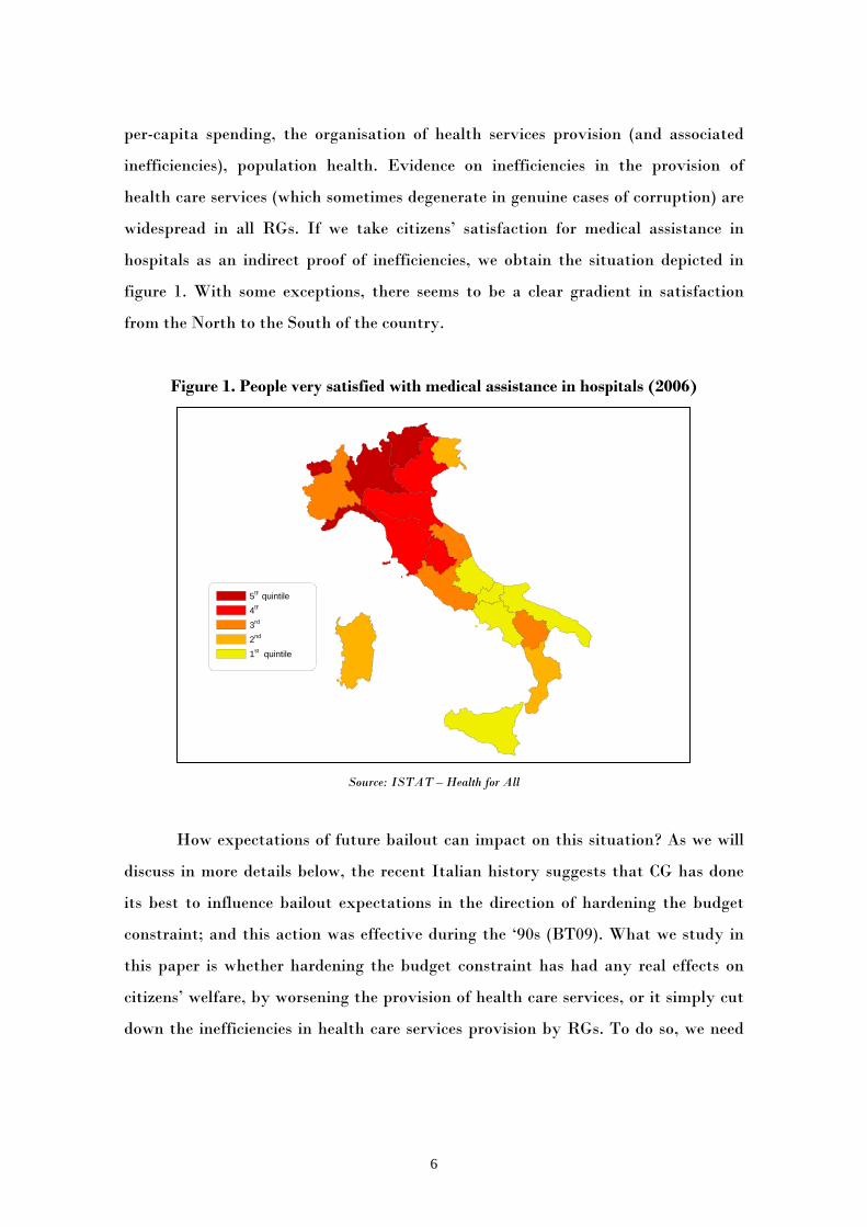
per-capita spending, the organisation of health services provision (and associated

inefficiencies), population health. Evidence on inefficiencies in the provision of

health care services (which sometimes degenerate in genuine cases of corruption) are

widespread in all RGs. If we take citizens’ satisfaction for medical assistance in

hospitals as an indirect proof of inefficiencies, we obtain the situation depicted in

figure 1. With some exceptions, there seems to be a clear gradient in satisfaction

from the North to the South of the country.

Figure 1. People very satisfied with medical assistance in hospitals (2006)

Source: ISTAT – Health for All

How expectations of future bailout can impact on this situation? As we will

discuss in more details below, the recent Italian history suggests that CG has done

its best to influence bailout expectations in the direction of hardening the budget

constraint; and this action was effective during the ‘90s (BT09). What we study in

this paper is whether hardening the budget constraint has had any real effects on

citizens’ welfare, by worsening the provision of health care services, or it simply cut

down the inefficiencies in health care services provision by RGs. To do so, we need

5th quintile 4th

3rd

2nd

1st quintile

7

both to ‘measure’ expectations in some ways, and to separate efficient from

inefficient spending. We approach these two problems in turn.

3. Theoretical framework: the intergovernmental game

In order to ‘measure’ expectations, in this section we briefly sketch a theoretical

framework useful for the following empirical analysis. We borrow entirely from

BT09, that provide some fundamental predictions for our test on the effects of

bailout expectations on citizens’ well-being5.

The authors consider a dynamic game with incomplete information; there are

two players (here levels of government), a CG and a RG. The timing of the game

strictly mirrors the relationships in the Italian NHS: at the first stage, CG finances

RG, by choosing between two levels of funding (F), low or high, F= {FL, FH}, where

FH>FL>0. At the second stage of the game, having observed F, RG can then decide

between two levels of expenditure (E), low or high, E = {EL, EH}, where EH>EL>0.

Notice that, if RG replies with the corresponding level of expenditure to the funding

decision of the CG, the regional budget is in equilibrium: (FH – EH) = (FL – EL) = 0,

and the game ends here. In fact, assuming RG cannot cash the difference between

expenditure and funding implies that, if CG sets FH at the beginning of the game,

then RG can only respond by setting EH. On the contrary, when CG sets FL at the

first stage of the game, RG can either react by setting EL (and the game is again

over), or by choosing EH and running a deficit. In this case, it is again CG’s turn to

move in the third stage of the game. It can either refuse to accommodate the deficit;

or it can accommodate, partly or fully, this increased regional expenditure by giving

more money to the region.

BT09 assume that: i) CG prefers low financing and low expenditure, both

when the bailing out occurs and when it does not; ii) RG prefers high expenditure

and high financing (and the sooner the better), but if it had to finance itself the

deficit in the case of low financing, it would prefer to cut expenditure immediately;

5 Notice that here we just sketch the essential characteristics of the model. We refer interested readers to the original paper for formal details.

8

iii) it is Pareto-efficient to constrain funding and expenditure at the low level – hence

EL is the structural expenditure, i.e., the level of spending necessary to guarantee

citizens’ well-being, while [EH – EL] identifies spending inefficiency; iv) there are two

possible types of CG: a ‘tough’ CG, and a ‘weak’ CG. The ‘tough’ type will enforce

fiscal discipline towards sub-national governments, and will not bail out RG deficit.

On the contrary, the ‘weak’ CG will easily indulge in bailouts. The type is a private

information of CG, hence RG needs to form some expectations on CG type: RG

expects to face a ‘tough’ CG with a positive probability p.

As shown by BT09, the Perfect Bayesian Equilibria of this game imply the

following: a ‘weak’ CG can take advantage of RG uncertainty by mimicking the ‘tough’

type, since – if it can convince RG that it is ‘tough’ – it might reach the Pareto-efficient

outcome, i.e., a low level of funding coupled with a low level of expenditure, hence a

situation without any deficits. From this result, the following testable implications

can be derived:

(a) ceteris paribus, it should be more likely to observe a low level of ex-ante CG funding

FL when p is high than when p is low;

(b) having observed a low level of ex-ante funding FL, RG is more likely to react with a

low level of health expenditure EL, when p is high than when p is low.

In other words, when the probability p to face a ‘tough’ CG is high, a low level of ex-

ante funding is perceived as a more reliable signal that CG is indeed ‘tough’;

therefore, RG reacts by choosing a low level of spending. Jointly considered, these

two theoretical predictions suggest to investigate the effects of bailout expectations

on RGs spending performance by testing the impact of ‘expected’ funding, i.e., ex-

ante CG funding conditional to RGs expectations on p. The crucial empirical problem

– to be discussed next – is how to find proper proxies for changes in p.

3.1. Linking the theory to the data

Changes in p mean a shift in bailout expectations, due to a strengthening of CG’s

commitment technology: when it is more costly for CG itself to run deficits (due for

instance to external constraints) and when there are new tools for RGs to respect

9

their budget (for instance, because of larger own resources, or an electoral system

that increase the accountability of local politicians), then the probability to face a

‘tough’ CG increases. The problem is how to model this shift.

We follow here BT09 and exploit a ‘quasi-natural experiment’ in Italy. In

particular, the link between theoretical model and observable variables is based on

the consideration of key events in the Italian economic history starting from the

‘90s, and their potential impact on p. The list includes the following events:

• 1992: a severe financial crisis, determined by an unsustainable level of both public

deficit and public debt, which lead the country close to default and opened the door

to a season of reform;

• 1993: a structural reform of the NHS, which introduced more autonomy for Local

Health Units in charge of providing services to citizens, and separated the third

party payer from hospitals (the providers of services), to create a quasi-market

competition similar to the one experienced in the English NHS;

• 1994: a reform of the National voting system, with the aim of strengthening CG

and its ability to implement reform and manage the public budget (notice that

duration of government during the ‘80s was less than one year);

• 1995: a reform of the Regional voting system, with the aim of increasing the

accountability of Regional Governors in charge of managing resources for health

care (notice that approximately 80% on average of regional expenditures are for

health care services);

• 1997: the ‘Maastricht test’, that is the provision of the Maastricht Treaty – ratified

at the end of 1993 – to examine EU countries in order to define the first group of

participants to the European monetary union (EMU) and the adoption of the Euro.

The test was mainly based on two parameters of public finances sustainability,

specifically the debt-to-GDP ratio < 60% and the deficit-to-GDP ratio < 3%;

• 1997: the introduction of a new regional tax (IRAP), aimed at reducing vertical

imbalance, and at increasing regional accountability;

10

• 1998: the provisions of the Amsterdam Treaty (better known as the Stability and

Growth Pact, SGP from now on), which define conditions for remaining in the EMU.

In particular, a close-to-zero deficit was required in the medium run; in any case,

public deficit-to-GDP ratio cannot be more than 3%.6

Starting from the above list of key events, we define a set of proxies for

changes in p, i.e. the probability to observe a ‘tough’ CG, defining a list of variables

that should have had an impact on the commitment technology of CG. The proxies

we use in the following empirical analysis are:

a) an index of Public Budget Tightness (PBT), defined as the ratio between the

Italian deficit and the average EU deficit, to capture potential variations in the

way external constraints are imposed. For instance, if all EU countries share the

same fiscal difficulties, a political decision could be made to soften financial rules.

Indeed, this is exactly what happened at the beginning of the new century with

the rules imposed by the SGP;

b) a dummy to capture the effects of external constraints imposed by the

Maastricht Treaty (DMAAS = 1 from 1994 to 1997);

c) a dummy for the 1997 EMU exam (DEUR = 1 in 1997), to capture the differential

impact of the ‘exam year’ with respect to the rules imposed by the Maastricht

Treaty;

d) a dummy to capture the effects of external constraints imposed by the SGP (or

Amsterdam Treaty, DAMST = 1 for the periods 1998-2003 and 2005-2006; notice

that we excluded 2004, because provisions by the SGP were suspended in that

year);

6 Differently from the Maastricht Treaty, the Stability and Growth Pact has experienced several difficulties: provisions has been suspended for some years, after fiscal crises affecting Germany and France. After this suspension, European Governments struggled to reach a new agreement. The newly reformed Pact contains provisions conditional on the public finance of each country and taking into account cyclical considerations, all of which suggest more politically oriented judgements than technical rules. More on this point will be discussed below.

11

e) a proxy for the per capita tax base of regional taxes (TAXBASE), to capture the

impact due to an increase in regional own resources registered during the sample

period;

f) a dummy to control for ‘political alignment’ effects (DGOV = 1 if RG and CG

coalitions in power are the same), to capture the potential impact of friendly

governments in terms of a more generous funding (when monies are available) or

a more effective control on expenditure (when fiscal discipline is required).

Notice that proxies (a) to (d) show time variability only, while proxies (e) and (f)

show both time and cross-section variability. This means that proxies (a) to (d),

basically the rules imposed by the EU, affect all Regions contemporaneously and in

the same way; on the contrary, proxies (e) and (f) affect different Regions in

different ways. Hence, expectations are different for different Regions.

4. Empirical analysis

4.1. Data and empirical strategy

The empirical analysis is based on a balanced panel of the 15 Italian Ordinary

Statute Regions over the years 1993-20067. The main source of data is the official

database Health for All managed by the Italian Central Institute of Statistics

(ISTAT), integrated with information extracted from the Supplements to the

Statistical Bulletin by the Bank of Italy, and the General Report on the Economic

Situation of the Country (Relazione Generale sulla Situazione Economica del Paese)

by the Italian Ministry of the Economy. All financial variables are expressed in 2006

€ per capita by using a CPI index.8

7 As already mentioned, we excluded from the analysis the five Special Statute Regions (Valle d’Aosta, Trentino Alto Adige, Friuli Venezia Giulia, Sardegna, Sicilia), because the way they are financed and they can organise the provision of health services follows different rules. In particular, «they enjoy wider autonomy [in the choice to allocate CG funds], and also receive a higher than average share of government funding. In addition, their self-government rights extend to an additional number of policy areas, such as primary and secondary education, culture and arts and subsidies to industry, commerce and agriculture» (Rico and Cetani, 2001: p. 5) 8 A sector specific retail price index is unavailable. However, the use of a general CPI index seems more appropriate, since most of the health care services are provided free of charge to citizens and the biggest expenditure share (personnel costs) varies according to the CPI index.

12

As for the empirical strategy, we work within the ‘substitution method’

suggested by BT09. The main objective of the paper is to test theoretical claim (b)

that, after having observed a low level of ex-ante CG funding, RGs should be more

likely to react with a low spending level the higher is p, and, more importantly, to

verify whether changes in p (i.e., in bailout expectations) impact the efficient

component and/or the waste component of overall spending. Since CG funding is not

exogenously given, but – according to the theoretical framework sketched above –

depends itself on the commitment technology available for CG, we need to go along

the following steps:

• we first check the effects of changes in p on ex-ante CG funding (FUNDST), by

estimating a model of funding which includes the proxies for bailout expectations

discussed above among the regressors;

• we then get ‘expected’ funding (i.e., predicted ex-ante CG funding given changes in

p) from first step estimates and insert this variable (EXPFUNDST) in a proper health

production function/frontier;

• we check whether EXPFUNDST affects structural expenditure (hence, citizens’

health) and/or inefficiency (hence, excess spending given a certain health output).

4.2. Modelling ex-ante central government funding

We define – differently from BT09 – the variable FUNDST as the difference between

total funding and regional funding. This is a measure of the ex-ante CG transfers per

capita to each Region, i.e. the topping up on regional own resources which

constitutes the first step in regional health care funding. We then estimate the

following CG funding model [1]:

FUNDSTit = a0 + a1TAXBASEit + a2PBTt + a3DGOVit + a4DEURt

+ a5DMAASt + a6DAMSTt + a7TRENDt + ∑=

14

1iiα REGi + εit [1]

i = 1, ..., 15; t = 1993, ..., 2006

13

where REG are individual fixed-effects, to take into account structural differences in

health spending needs across RGs, and TREND is a linear trend that captures the

evolution of ex-ante CG funding linked to the dynamics of expenditure reflecting

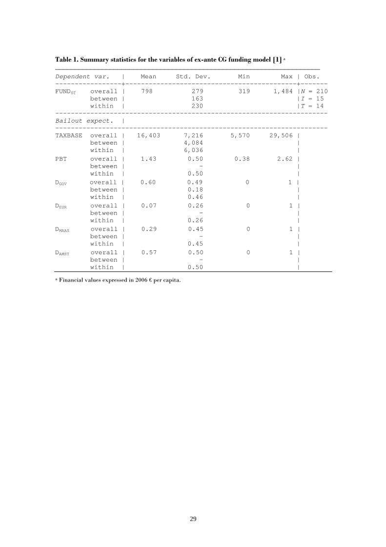
technical progress in health care delivery (see section 4.3). Table 1 reports descriptive

statistics for the variables included in Eq. [1].

[INSERT TABLES 1 AND 2 HERE]

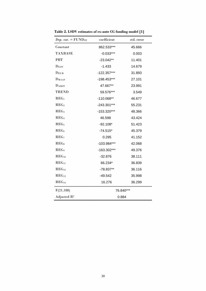
Table 2 shows Least Square Dummy Variable (LSDV) estimates of ex-ante

CG funding model [1]. All proxies for changes in bailout expectations – but DGOV9 –

are strongly statistically significant and show a sign consistent with our a priori and

previous findings by BT09. An increase in the tax base given to regions should

increase their ability to cope autonomously with their deficits, and this should make

more credible the threat by CG not to bail them out (hence, the coefficient of

TAXBASE < 0). As Maastricht requirements become more binding, CG should be

perceived as tougher (hence, the coefficient of DMAAS < 0), and this effect should be

more important the higher the Italian deficit with respect to the EU average (hence,

the coefficient of PBT < 0), and the closer the deadline for the admission test to be

included in the first group of countries adopting the Euro (hence, the coefficient of

DEUR < 0). On the other hand, the positive impact exerted on CG funding by the

introduction of the SGP (coefficient of DMAAS > 0) may be explained by the

weaknesses of the Amsterdam Treaty in itself compared to the provisions of the

Maastricht Treaty. These fragilities led European governments to perceive the

threat of exclusion from the EMU as an unlikely event, and – in turn – brought RGs

to increase their expectations of future bailouts by CG.10

9 Perhaps a ‘help out’ action by friendly Regions – aimed at cooperating with CG in controlling public expenditure and deficit – arose until 1997, before the ‘Maastricht test’ (like in BT09), whilst an opposite effect prevailed from 1998, due to RGs expectations of a more ‘benevolent’ treatment in terms of ex-post funding by a friendly CG than by an adversary one. See Arulampalan et al. (2009) for further discussion on this issue. 10 Notice that the possibility that some member states might in the future obtain back their monetary sovereignty is not even considered in European Treaties. As argued by Bordignon and Brusco (2001), the absence of explicit provisions can be seen as a commitment device to increase stability. However, the increased stability can probably lower the expectations that penalties and automatic sanctions

14

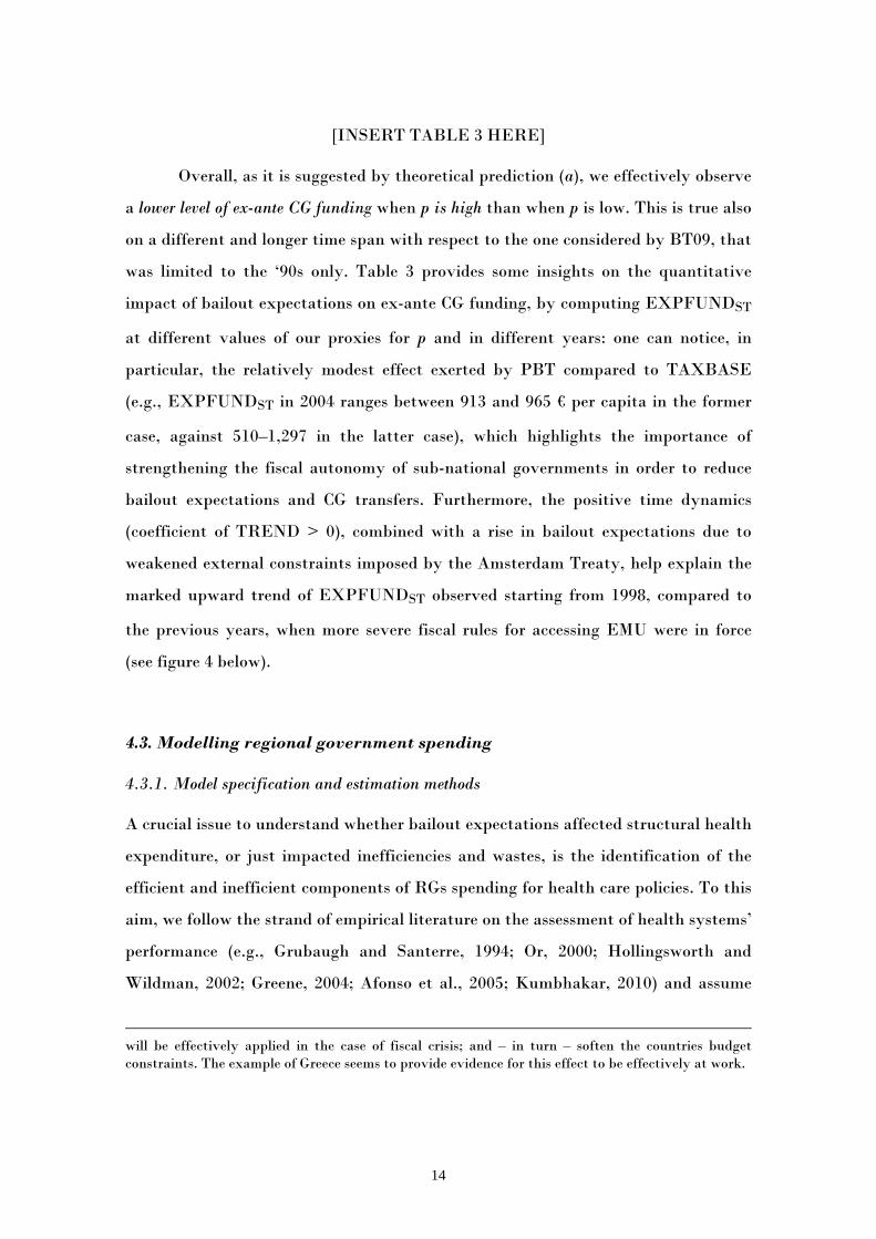
[INSERT TABLE 3 HERE]

Overall, as it is suggested by theoretical prediction (a), we effectively observe

a lower level of ex-ante CG funding when p is high than when p is low. This is true also

on a different and longer time span with respect to the one considered by BT09, that

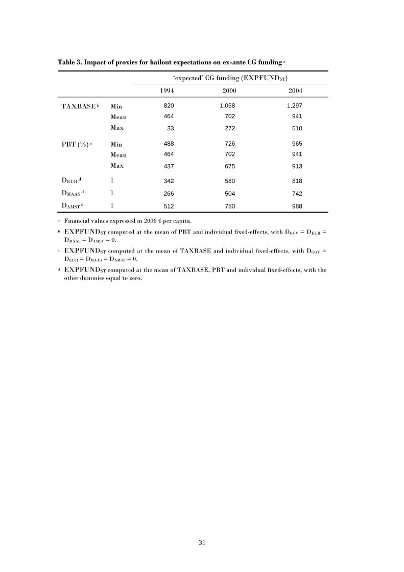
was limited to the ‘90s only. Table 3 provides some insights on the quantitative

impact of bailout expectations on ex-ante CG funding, by computing EXPFUNDST

at different values of our proxies for p and in different years: one can notice, in

particular, the relatively modest effect exerted by PBT compared to TAXBASE

(e.g., EXPFUNDST in 2004 ranges between 913 and 965 € per capita in the former

case, against 510–1,297 in the latter case), which highlights the importance of

strengthening the fiscal autonomy of sub-national governments in order to reduce

bailout expectations and CG transfers. Furthermore, the positive time dynamics

(coefficient of TREND > 0), combined with a rise in bailout expectations due to

weakened external constraints imposed by the Amsterdam Treaty, help explain the

marked upward trend of EXPFUNDST observed starting from 1998, compared to

the previous years, when more severe fiscal rules for accessing EMU were in force

(see figure 4 below).

4.3. Modelling regional government spending

4.3.1. Model specification and estimation methods

A crucial issue to understand whether bailout expectations affected structural health

expenditure, or just impacted inefficiencies and wastes, is the identification of the

efficient and inefficient components of RGs spending for health care policies. To this

aim, we follow the strand of empirical literature on the assessment of health systems’

performance (e.g., Grubaugh and Santerre, 1994; Or, 2000; Hollingsworth and

Wildman, 2002; Greene, 2004; Afonso et al., 2005; Kumbhakar, 2010) and assume

will be effectively applied in the case of fiscal crisis; and – in turn – soften the countries budget constraints. The example of Greece seems to provide evidence for this effect to be effectively at work.

15

that health policy outcomes result from a standard microeconomic ‘production

function’, where health care is the output, spending and other health-related

variables are the inputs, and a process of optimization underlies the observed data.

However, we depart here from the bulk of previous studies, which assumes

health care maximization given a certain amount of health expenditure, ceteris

paribus, as the objective to be pursued by the policy maker. Indeed, considering the

rapid growth in health spending for all European countries in the last decades, the

significantly higher level of output compared to less developed contexts (e.g., in

terms of average life expectancy), and the role played by public finance constraints

imposed by European rules, we believe it is more correct to define an alternative goal

for RGs, which consists in minimizing the cost (i.e., public health expenditure) of

providing a certain level of health output, given other inputs and a set of control

variables. According to the approach adopted in Kumbhakar (2010) to analyse

WHO member countries’ health systems, this issue can be addressed by modelling

RGs spending behavior as an input requirement function. This concept was first

introduced by Diewert (1974), and later extended by Kumbhakar and Hjalmarsson

(1995) to incorporate inefficiency in the production process, i.e., the use of excess

input compared to the optimal (minimum) need defined by a best-practice frontier.11

The identification of a proper output for quantifying the outcome of health

care policies is a rather difficult issue, because the effectiveness of health services can

be assessed by considering a variety of aspects (e.g., length and quality of life, equity

in accessing the services, etc). Accordingly with most of the past studies on health

systems’ efficiency12, we adopt two traditional measures of health attainment and

proxy the output (Y) both as average life expectancy at birth (ALE) and infant

mortality rate (IMR).13 As for the basic inputs of health production process, per

11 For a comprehensive and critical review of the literature on production/cost frontier modelling and efficiency measurement, see the handbooks by Kumbhakar and Lovell (2000) and Coelli et al. (2005). 12 See, among others, Grubaugh and Santerre (1994), Or (2000), Retzlaff-Roberts et al. (2004), Afonso et al. (2005), and Porcelli (2009). 13 Life expectancy is the average number of years of life remaining at a given age and, in the database Health for All, it is computed separately for men and women. Therefore, male and female life expectancies at birth have been averaged by male and female populations, in order to obtain a single

16

capita public and private health care expenditure and average education level of the

population have been typically used in the existing literature. Coherently with this

strand of analysis, we define per capita RGs health spending (HPUB) as the

dependent variable of the input requirement function, and per capita private health

spending (HPRIV) and the percentage of people with higher education (EDUUNIV)14

as the other productive factors (INPUT).

In addition, we augment our specification with a set of control variables (CV )

that are likely to generate possible shifts in the production relationship, both over

time and across Regions.15 Specifically, we include: a time trend variable (TREND)

to take into account possible improvements in health care delivery over years due to

technical change; two demographic indicators, i.e., the share of males (MALE) and

of people older than 75 (OLD75), which are expected to exert a negative and positive

impact, respectively, on the minimum level of HPUB required to attain a given level

of Y, ceteris paribus16; a variable accounting for the effect of bailout expectations,

i.e., EXPFUNDST obtained from estimates of Eq. [1] (the way we test whether this

factor is a shifter of the frontier or affects the inefficiency is discussed later); finally,

given the wide variation in cultural and economic characteristics of our sample

(especially between Northern and Southern Regions), which is likely to influence

health policy outcomes, we incorporate individual fixed-effects (REG) in the

estimated model, so as to control for unobserved heterogeneity across Regions. Table

index. Infant mortality rate is given by the number of children who die during the first year of life per 10,000 newborns. Some recent studies (e.g., Hollingsworth and Wildman, 2002; Gravelle et al., 2003; Greene, 2004; Kumbhakar, 2010) have measured health outcomes in terms of Disability Adjusted Life Expectancy (DALE), an indicator of healthy life expectancy which differs from ‘pure’ life expectancy or mortality indices in that it considers the quality of life besides its length. However, information on DALE disaggregated at regional level is not available for the whole time-series of our panel. 14 This variable is computed as the share of persons with a university degree out of the total regional population. We thank Anna Laura Mancini for kindly providing these data. 15 Or (2000), Gravelle et al. (2003) and Greene (2004) argued about the importance to enrich the basic input-output relationship of the health production process, by adding further covariates able to account for some of the widespread heterogeneity that is usually present in this type of data. 16 The importance of technological change and demographic factors such as age and gender is widely debated in the empirical literature on health spending determinants. Chernichovsky and Markowitz (2004) provide a survey of main findings of these studies with and interesting analysis of the Israeli experience.

17

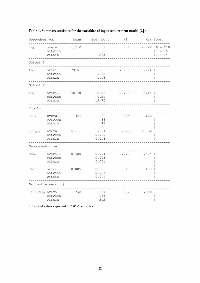
4 shows summary statistics for the variables included in the input requirement

function; to support the choice of using panel data methods, one can notice that

both the dependent variable and the regressors show enough variation in the data,

both over time and across Regions.17

[INSERT TABLE 4 HERE]

The functional form of the input requirement model remains to be defined. In

the interest of parsimony, we follow Or (2000) and Greene (2005b), among others, and

adopt a simple Cobb-Douglas specification.18 The model (in logarithmic form) to be

estimated is:

lnHPUBit = b0 + b1lnYit + b2lnHPRIVit + b3lnEDUUNIVit + b7TRENDt

+ b4lnMALEit+ b5lnOLD75it + b6lnEXPFUNDSTit + ∑=

14

1iiβ REGi + eit [2]

i = 1, ..., 15; t = 1993, ..., 2006

which can be concisely rewritten as:

lnHPUBit = f (lnYit, lnINPUTit, lnCVit ) + eit [3]

The residual term, eit, can be thought either 1) as pure random noise – like in a

standard average function approach, not accounting for the presence of productive

inefficiency in observed health spending – or 2) as a composed error term, resulting

from the sum of idiosyncratic noise (vit) and a nonnegative inefficiency term (uit) –

like in a frontier function approach, where actual health spending is allowed to

exceed the optimal (minimum) requirement. According to the latter interpretation, a

Region that is managing more efficiently the provision of health care will, ceteris

17 In particular, within variation is dominant for HPUB, ALE, IMR, EDUUNIV and EXPFUNDST, while the variation between Regions prevails in HPRIV, MALE and OLD75. 18 In principle, the flexible translog form should be used to approximate at best an arbitrary underlying function. However, due to the high multicollinearity among the regressors (which include interacted and squared terms) and the limited degrees of freedom, in past studies the translog specification often resulted in parameter estimates failing to satisfy some of the basic properties of production theory. Therefore, as remarked by Greene (2004, p. 968), a strictly orthodox interpretation of the relationship between the health outcomes and the inputs as perfectly conforming to a neoclassical production function is likely to be optimistic, and the use of looser approximations is then justified.

18

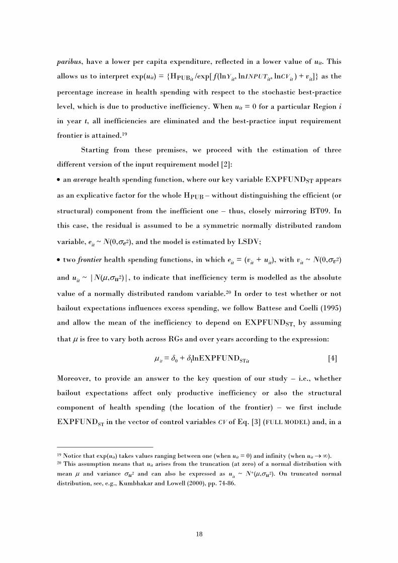
paribus, have a lower per capita expenditure, reflected in a lower value of uit. This

allows us to interpret exp(uit) = {HPUBit /exp[ f (lnYit, lnINPUTit, lnCVit ) + vit]} as the

percentage increase in health spending with respect to the stochastic best-practice

level, which is due to productive inefficiency. When uit = 0 for a particular Region i

in year t, all inefficiencies are eliminated and the best-practice input requirement

frontier is attained.19

Starting from these premises, we proceed with the estimation of three

different version of the input requirement model [2]:

• an average health spending function, where our key variable EXPFUNDST appears

as an explicative factor for the whole HPUB – without distinguishing the efficient (or

structural) component from the inefficient one – thus, closely mirroring BT09. In

this case, the residual is assumed to be a symmetric normally distributed random

variable, eit ~ N(0,σe2), and the model is estimated by LSDV;

• two frontier health spending functions, in which eit = (vit + uit), with vit ~ N(0,σv2)

and uit ~ |N(µ,σu2)|, to indicate that inefficiency term is modelled as the absolute

value of a normally distributed random variable.20 In order to test whether or not

bailout expectations influences excess spending, we follow Battese and Coelli (1995)

and allow the mean of the inefficiency to depend on EXPFUNDST, by assuming

that µ is free to vary both across RGs and over years according to the expression:

itµ = δ0 + δllnEXPFUNDSTit [4]

Moreover, to provide an answer to the key question of our study – i.e., whether

bailout expectations affect only productive inefficiency or also the structural

component of health spending (the location of the frontier) – we first include

EXPFUNDST in the vector of control variables CV of Eq. [3] (FULL MODEL) and, in a

19 Notice that exp(uit) takes values ranging between one (when uit = 0) and infinity (when uit → ∞). 20 This assumption means that uit arises from the truncation (at zero) of a normal distribution with mean µ and variance σu2 and can also be expressed as uit ~ N+(µ,σu2). On truncated normal distribution, see, e.g., Kumbhakar and Lowell (2000), pp. 74-86.

19

second frontier specification (RESTRICTED MODEL), we exclude it from CV (setting b6

= 0 in Eq.[2]). Then, we use a standard LR test for selecting the best specification.

In both cases, maximum likelihood (ML) is employed for the simultaneous

estimation of the stochastic frontier parameters [3] and the spending inefficiency

equation [4]. The log-likelihood function is formulated in terms of the

parameterization suggested by Battese and Corra (1977), who replace σv2 and σu2

with σ2 ≡ (σv2 + σu2) and γ ≡ σu2/(σv2 + σu2).21 The parameter γ must lie between 0

and 1 and provides useful information on the relative contribution of uit and vit to

the global residual eit, hence on the importance of estimating a best-practice frontier

instead of an average input requirement function, by separating inefficiencies from

structural spending.22 It is important to highlight that adding the full set of regional

dummies REG in the vector CV corresponds to implementing the ‘true’ fixed-effects

ML frontier model proposed by Greene (2004, 2005a,b), which has the virtue to

allow a distinction between the unobserved cross-region heterogeneity, unrelated to

inefficiency, and the inefficiency itself.23

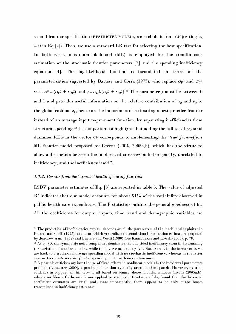
4.3.2. Results from the ‘average’ health spending function

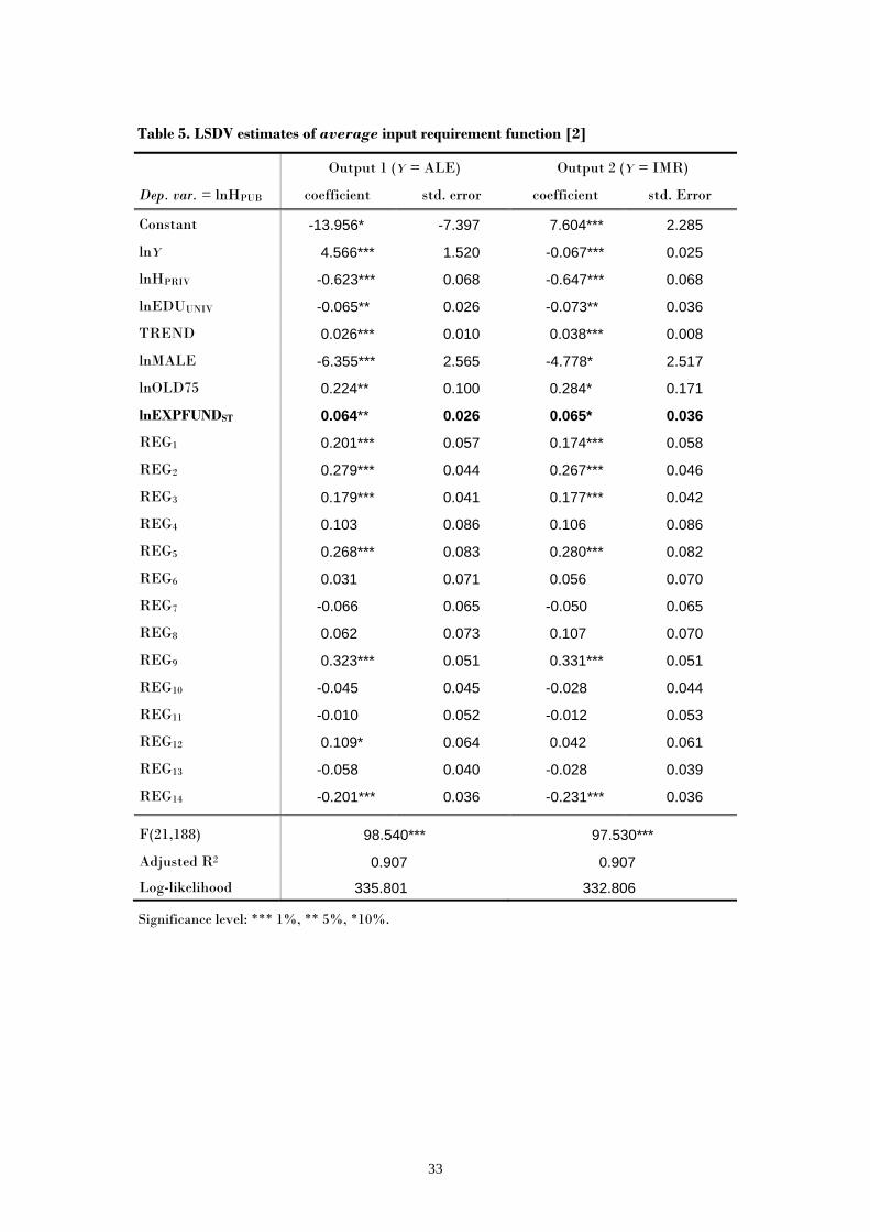
LSDV parameter estimates of Eq. [3] are reported in table 5. The value of adjusted

R2 indicates that our model accounts for about 91% of the variability observed in

public health care expenditure. The F statistic confirms the general goodness of fit.

All the coefficients for output, inputs, time trend and demographic variables are

21 The prediction of inefficiencies exp(uit) depends on all the parameters of the model and exploits the Battese and Coelli (1995) estimator, which generalizes the conditional expectation estimators proposed by Jondrow et al. (1982) and Battese and Coelli (1988). See Kumbhakar and Lowell (2000), p. 78. 22 As γ → 0, the symmetric noise component dominates the one-sided inefficiency term in determining the variation of total residual eit, while the inverse occurs as γ → 1. Notice that, in the former case, we are back to a traditional average spending model with no stochastic inefficiency, whereas in the latter case we face a deterministic frontier spending model with no random noise. 23 A possible criticism against the use of fixed effects in nonlinear models is the incidental parameters problem (Lancaster, 2000), a persistent bias that typically arises in short panels. However, existing evidence in support of this view is all based on binary choice models, whereas Greene (2005a,b), relying on Monte Carlo simulation applied to stochastic frontier models, found that the biases in coefficient estimates are small and, more importantly, there appear to be only minor biases transmitted to inefficiency estimates.

20

found to be statistically significant and their magnitude is quite similar for the two

model specifications using alternative output measures for health care policies (ALE,

IMR). Furthermore, the significance of a high number of regional dummies

(seven/six out of fourteen) supports the inclusion of individual fixed-effects in the

model to control for unmeasured cross-region heterogeneity. As expected, HPUB

increases with the targeted output (if Y = ALE; it clearly decreases if Y = IMR),

while it shows a certain degree of substitutability with private health spending and

with higher education. The latter result confirms evidence by Kumbhakar (2010)

and can be explained by the fact that people with higher education do more

prevention, demanding more preventive care, using non-medical inputs and leading

healthier life styles, so as to become more efficient users of care and producers of

health; thus, ceteris paribus, the effect of rising EDUUNIV is to reduce the aggregate

costs for health care.24

[INSERT TABLE 5 HERE]

The positive coefficient of TREND shows that RGs health spending increases

at an annual rate of about 3-4%. To some extent, this growth over time of HPUB is

due to changes in medical technology, implying better and more costly treatments.25

As for the impact of demographic factors, the negative coefficient of MALE

indicates that females are more likely to visit health providers than males26;

moreover, the positive effect of POP75 confirms that a rise in the share of the elderly

out of total population tends to cause higher health costs27, because of the increased

incidence of chronic diseases, as well as the closer proximity to death (Zweifel et al.,

1999).

24 For further discussion on this issue, see Chernichovsky and Markowitz (2004). 25 A similar finding has been obtained in a recent study on Swiss health care system by Filippini et al. (2006). In general, technical progress is considered an essential factor in rising health care costs (see Newhouse, 1992). 26 In particular, Chernichovsky and Markowitz (2004) point to a remarkable increase in the number of visits to doctors and specialists by females between 25 and 64 year old, and in the number of visits to nurses by females between 25 and 44 year old. 27 Evidence supporting this view is found, among others, in Giannoni and Hitiris (2002), Seshamani and Gray (2004), and Filippini et al. (2006).

21

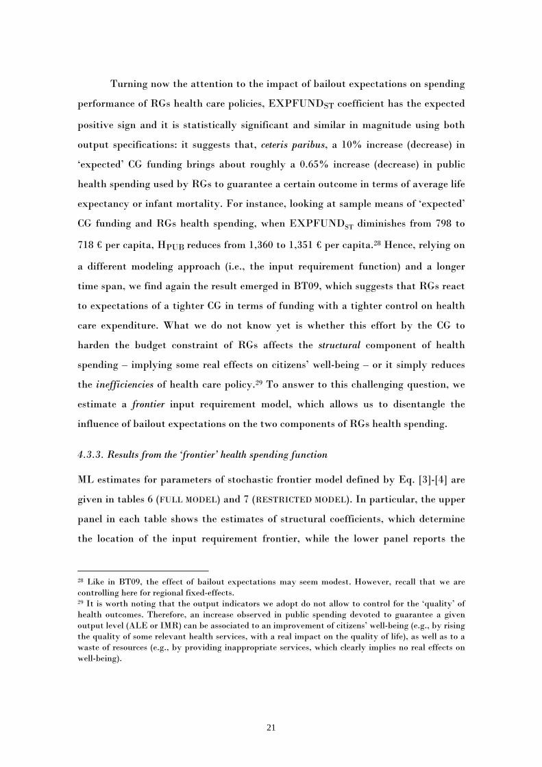
Turning now the attention to the impact of bailout expectations on spending

performance of RGs health care policies, EXPFUNDST coefficient has the expected

positive sign and it is statistically significant and similar in magnitude using both

output specifications: it suggests that, ceteris paribus, a 10% increase (decrease) in

‘expected’ CG funding brings about roughly a 0.65% increase (decrease) in public

health spending used by RGs to guarantee a certain outcome in terms of average life

expectancy or infant mortality. For instance, looking at sample means of ‘expected’

CG funding and RGs health spending, when EXPFUNDST diminishes from 798 to

718 € per capita, HPUB reduces from 1,360 to 1,351 € per capita.28 Hence, relying on

a different modeling approach (i.e., the input requirement function) and a longer

time span, we find again the result emerged in BT09, which suggests that RGs react

to expectations of a tighter CG in terms of funding with a tighter control on health

care expenditure. What we do not know yet is whether this effort by the CG to

harden the budget constraint of RGs affects the structural component of health

spending – implying some real effects on citizens’ well-being – or it simply reduces

the inefficiencies of health care policy.29 To answer to this challenging question, we

estimate a frontier input requirement model, which allows us to disentangle the

influence of bailout expectations on the two components of RGs health spending.

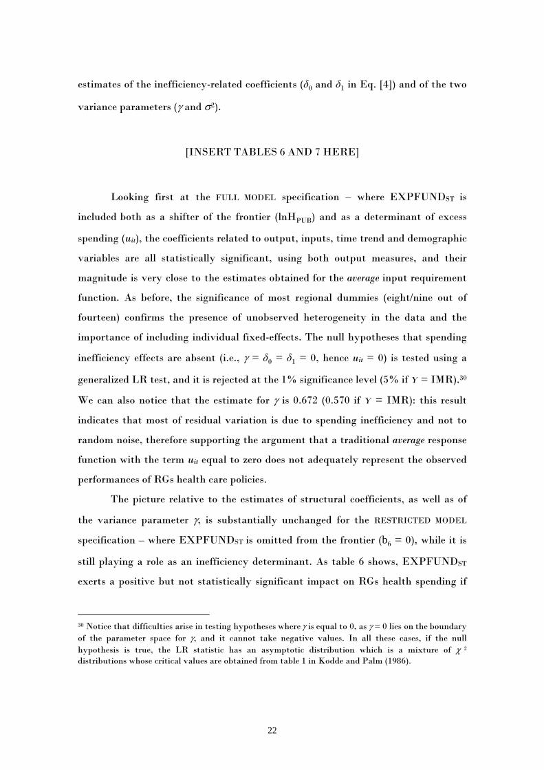
4.3.3. Results from the ‘frontier’ health spending function

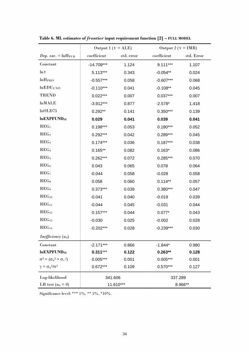
ML estimates for parameters of stochastic frontier model defined by Eq. [3]-[4] are

given in tables 6 (FULL MODEL) and 7 (RESTRICTED MODEL). In particular, the upper

panel in each table shows the estimates of structural coefficients, which determine

the location of the input requirement frontier, while the lower panel reports the

28 Like in BT09, the effect of bailout expectations may seem modest. However, recall that we are controlling here for regional fixed-effects. 29 It is worth noting that the output indicators we adopt do not allow to control for the ‘quality’ of health outcomes. Therefore, an increase observed in public spending devoted to guarantee a given output level (ALE or IMR) can be associated to an improvement of citizens’ well-being (e.g., by rising the quality of some relevant health services, with a real impact on the quality of life), as well as to a waste of resources (e.g., by providing inappropriate services, which clearly implies no real effects on well-being).

22

estimates of the inefficiency-related coefficients (δ0 and δ1 in Eq. [4]) and of the two

variance parameters (γ and σ2).

[INSERT TABLES 6 AND 7 HERE]

Looking first at the FULL MODEL specification – where EXPFUNDST is

included both as a shifter of the frontier (lnHPUB) and as a determinant of excess

spending (uit), the coefficients related to output, inputs, time trend and demographic

variables are all statistically significant, using both output measures, and their

magnitude is very close to the estimates obtained for the average input requirement

function. As before, the significance of most regional dummies (eight/nine out of

fourteen) confirms the presence of unobserved heterogeneity in the data and the

importance of including individual fixed-effects. The null hypotheses that spending

inefficiency effects are absent (i.e., γ = δ0 = δ1 = 0, hence uit = 0) is tested using a

generalized LR test, and it is rejected at the 1% significance level (5% if Y = IMR).30

We can also notice that the estimate for γ is 0.672 (0.570 if Y = IMR): this result

indicates that most of residual variation is due to spending inefficiency and not to

random noise, therefore supporting the argument that a traditional average response

function with the term uit equal to zero does not adequately represent the observed

performances of RGs health care policies.

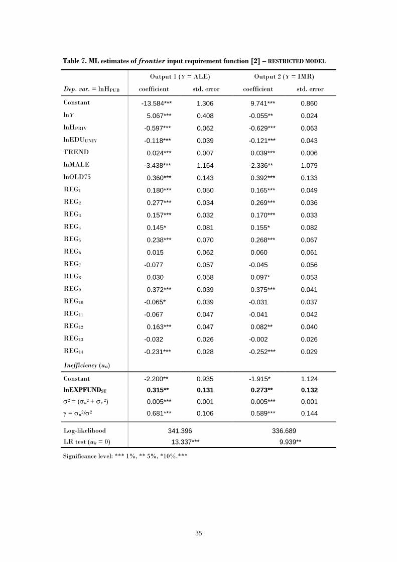
The picture relative to the estimates of structural coefficients, as well as of

the variance parameter γ, is substantially unchanged for the RESTRICTED MODEL

specification – where EXPFUNDST is omitted from the frontier (b6 = 0), while it is

still playing a role as an inefficiency determinant. As table 6 shows, EXPFUNDST

exerts a positive but not statistically significant impact on RGs health spending if

30 Notice that difficulties arise in testing hypotheses where γ is equal to 0, as γ = 0 lies on the boundary of the parameter space for γ, and it cannot take negative values. In all these cases, if the null hypothesis is true, the LR statistic has an asymptotic distribution which is a mixture of χ

2 distributions whose critical values are obtained from table 1 in Kodde and Palm (1986).

23

included as a structural variable (the p-value for b6 is 0.49 if Y = ALE, 0.34 if Y =

IMR), whereas its associated coefficient δl appears always highly significant when

bailout expectations are assumed to influence excess spending (at 1% level if Y =

ALE, 5% if Y = IMR), both in the restricted and full specifications. Thus, as these

are two nested models, we compare the full specification of the frontier input

requirement function against the restricted model by means of a standard LR test:

as we find no evidence to reject the RESTRICTED MODEL31, we are allowed to conclude

that bailout expectations do not significantly affect the position of the best-practice

frontier (hence, they should not influence citizens’ well-being), while they seem to

have a remarkable impact on spending inefficiency. The following comments, which

discuss more in depth inefficiency estimates and the role played by EXPFUNDST,

rely then on the results from the restricted specification (table 7).

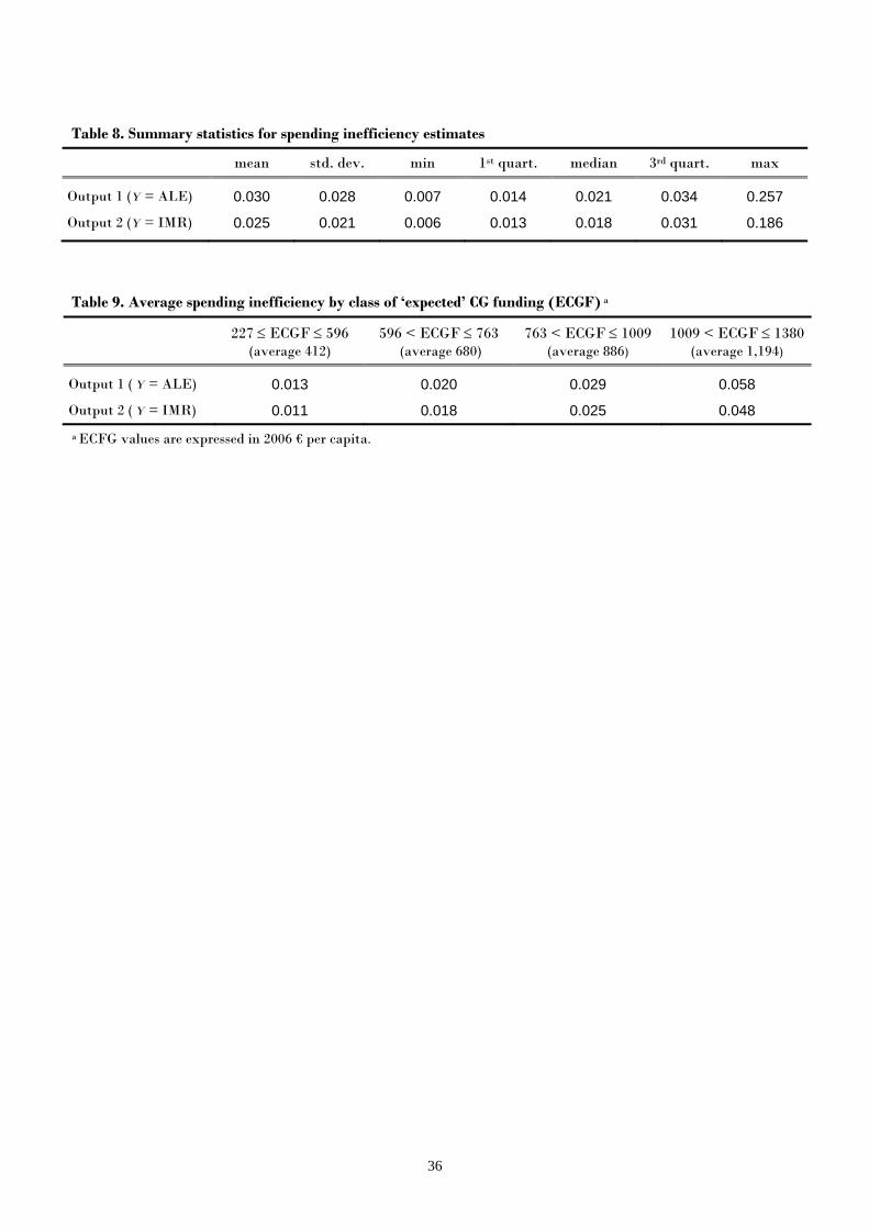
[INSERT TABLES 8 AND 9 HERE]

Table 8 provides summary statistics for estimated inefficiencies.32 Excess

spending ranges between 0.7% if Y = ALE (0.6% if Y = IMR) and 25.7% (18.6%),

and average cost inefficiency is found to be 3% (2.5%).33 Considering the sample

mean value of HPUB (1,360 €), this implies that RGs could reduce their health

spending by 40 € per capita (34 € if Y = IMR) by taking care of all the wastes in

health services delivery.34 Since our primary concern is with the effects of

expectations of deficit bailout by CG – here assessed looking at ‘expected’ CG

funding – table 9 shows the values of average inefficiency computed within different

31 The p-value for the LR statistic is 0.517 if Y = ALE and 0.273 if Y = IMR. 32 Estimates of spending inefficiency for each RG in each year are reported in tables A1-A2 in the Appendix. 33 The quite low values of spending inefficency may be due to a second potential issue concerning the use of the true fixed effects model, i.e., the possibility that the inefficiency terms are underestimated. Indeed, if there is some region-specific persistent inefficiency, it is absorbed by the regional dummy included in the frontier, which is also capturing any time invariant heterogeneity. Unfortunately, as remarked by Greene (2004, p. 964), there is no simple solution to this problem, since the blending of inefficiency and unobserved heterogeneity is intrinsic to this modelling approach. 34 Given the total Italian population of 60,045,068 inhabitants in 2008, this average efficiency recovery on per capita health spending would amount to an aggregate saving of about 2.5 billions € (2 billions € if Y = IMR).

24

classes of EXPFUNDST defined by the following ranges: min-1st quartile, 1st quartile-

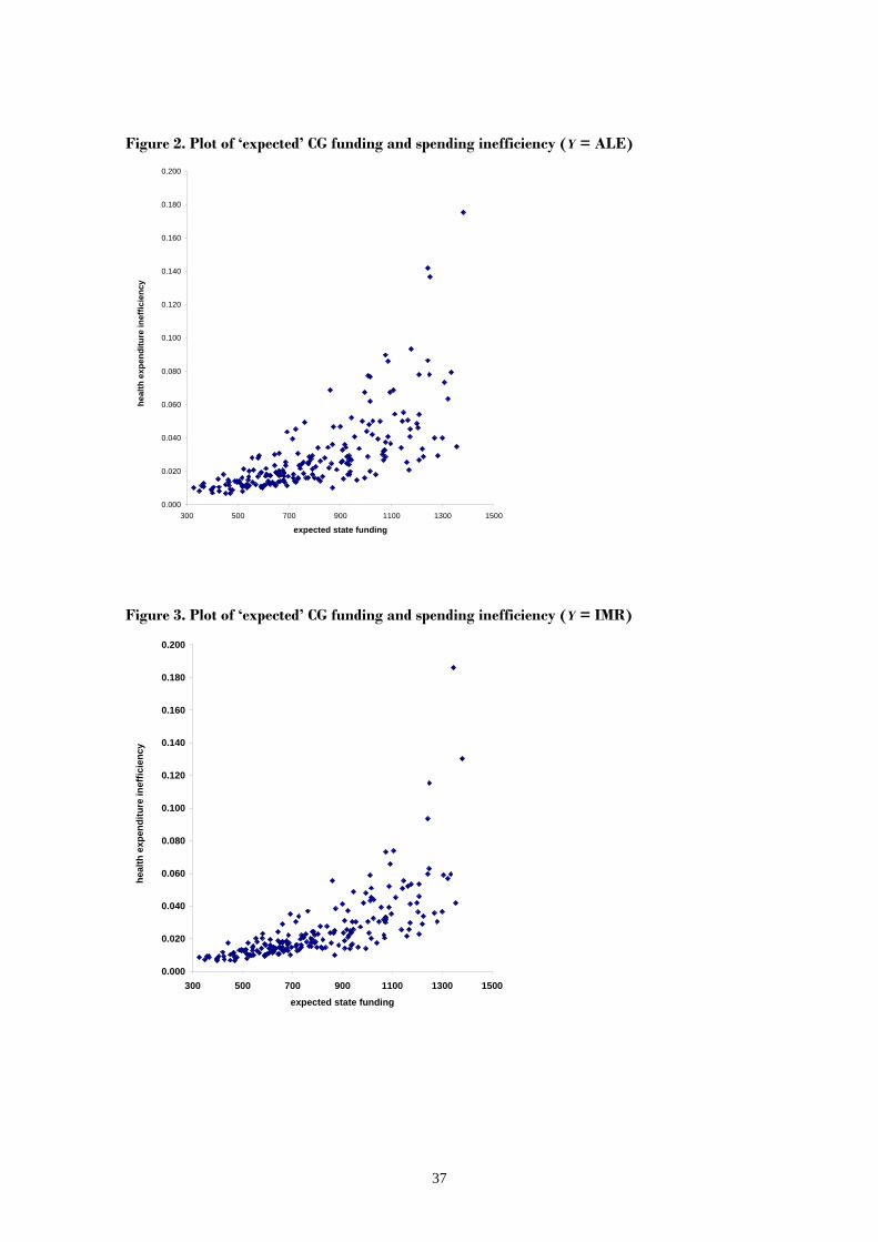
median, median-3rd quartile, 3rdquartile-max. The positive impact of bailout

expectations on excess spending is well highlighted by the more-than-proportional

increase of average cost inefficiency with the growth of EXPFUNDST: when

EXPFUNDST raise from a low (412 € per capita, on average) to a high level (1,194 €

per capita, on average), we observe cost inefficiencies to augment from 1% to about

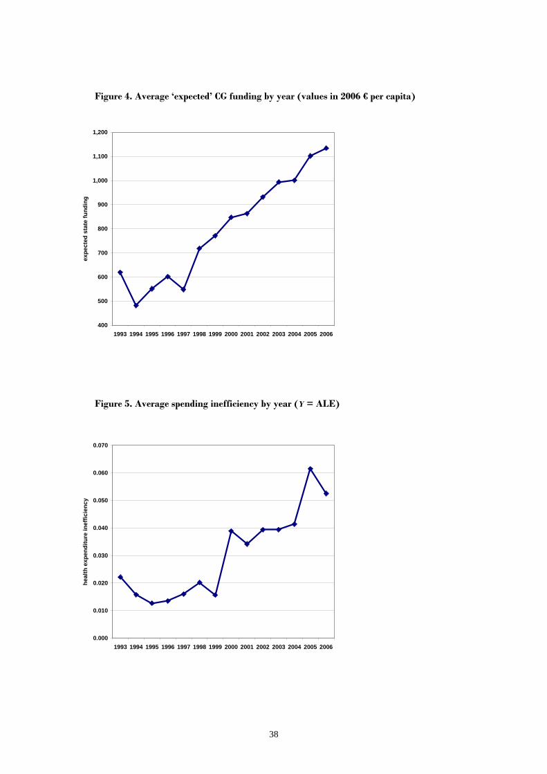
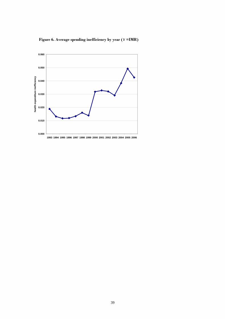
6% if Y = ALE (5% if Y = IMR). Figures 2-6 provide further evidence in support of

increasing excess spending in correspondence of higher levels of ‘expected’ CG

funding. In particular, the yearly trend of average cost inefficiency (computed using

both output indicators) and EXPFUNDST suggests that fiscal discipline by CG

towards RGs was effective in containing wastes during the mid ‘90s, when more

severe rules for accessing EMU were in force. Starting from the end of the ‘90s,

however, ex-ante CG funding – conditional to RGs expectations on p – began again

to increase permanently, to some extent because of the weaker external constraints

imposed by the SGP; with this growth of ‘expected’ CG funding, also health

spending inefficiency sharply augmented.

[INSERT FIGURES 2-6 HERE]

Taken together, these findings are strongly in favour of the idea that lower

bailout expectations, due to a more severe fiscal discipline by CG, have an influence

only on regional excess spending, and have no real effects on citizens’ well-being.

Therefore, enforcing fiscal discipline towards sub-national governments is expected

to result in welfare improvements.

5. Concluding remarks

This paper investigates whether fiscal discipline towards sub-national governments,

in order to harden their budget constraints, exerts any real effects on the well-being

of the citizens or simply helps to reduce waste of public monies. We consider the

provision of health care services by Italian Regions, a policy which is determined by

a complex net of intergovernmental relations and can strongly influence citizens’

25

welfare. We build on Bordignon and Turati (2009): besides extending the time span

considered in their analysis, we propose here to separate the efficient (or structural)

component of regional health spending from the inefficient one (excess spending), by

estimating a frontier input requirement function. This modelling approach allows us

to check whether bailout expectations – used as an indicator of the effort by Central

Government to induce fiscal discipline in Regional Governments – influence only

spending inefficiencies or they have any real effects on citizens’ health.

Our empirical analysis provides at least two interesting findings: first, there is

evidence confirming that ex-ante Central Government funding is heavily affected by

bailout expectations, and this suggests that Central Government can enforce fiscal

discipline towards sub-national governments by fixing the level of funding. Second,

and most importantly, controlling for other relevant inputs in the production of

health (private health expenditure and education) and for environmental factors

(demographic structure of the population, technological change, and region-specific

individual effects), ‘expected’ funding (i.e., Central Government transfers conditional

on expectations of deficit bailouts) influences only inefficient spending of Regional

Governments. Fiscal discipline appears then effective in reducing wastes, without

having any real effect on citizens’ health, one of the main facets of individual well-

being. Whether this matters also for other welfare sectors (e.g., social care,

education), and other countries where these policies are decentralised towards sub-

national governments as well, is an appealing issue for future research.

26

References

Afonso A., Schuknecht L. and Tanzi V. (2005), “Public sector efficiency: an

international comparison”, Public Choice, 123(3), 321–347.

Arulampalan W., Dasgupta S., Dhillon A. and Dutta B. (2009), “Electoral goals and

centre-state transfers: a theoretical model and empirical evidence from India”,

Journal of Development Economics, 88, 103–119.

Battese G.E. and Coelli T.J. (1988), “Prediction of firm-level technical efficiencies

with a generalized frontier production function and panel data”, Journal of

Econometrics, 38, 387–399.

Battese G.E. and Coelli T.J. (1995), “A model for technical inefficiency effects in a

stochastic frontier production function for panel data”, Empirical Economics, 20,

325–232.

Battese G.E. and Corra G.S. (1977), “Estimation of a production frontier model with

application to the pastoral zone of eastern Australia”, Australian Journal of

Agricultural Economics, 21, 169–179.

Besfamille M. and Lockwood B. (2008), “Bailouts in federations: is a hard budget

constraint always best?”, International Economic Review, 49(2), 577–593.

Bordignon M. and Brusco S. (2001), “Optimal secession rules”, European Economic

Review, 45, 1811–1834.

Bordignon M. and Turati G. (2009), “Bailing out expectations and public health

expenditure”, Journal of Health Economics, 28, 305–321.

Capps C., Dranove D. and Lindrooth R.C. (2010), “Hospital closure and economic

efficiency”, Journal of Health Economics, 29, 87-109.

Chernichovsky D. and Markowitz S. (2004), “Aging and aggregate costs of medical

care: conceptual and policy issues”, Health Economics, 13, 543–562.

Coelli T.J., Prasada Rao D.S., O’Donnell C.J. and Battese G.E. (2005), An

introduction to efficiency and productivity analysis, 2nd edition, Springer, New

York.

27

Crivelli L., Filippini M. and Mosca I. (2006), “Federalism and regional health care

expenditures: an empirical analysis for the Swiss cantons”, Health Economics, 15,

535–541.

Diewert E. (1974), “Applications of duality theory”, in M. Intriligator and D.

Kendrick (eds.), Frontiers in Quantitative Economics, Amsterdam: North Holland.

Giannoni M. and Hitiris T. (2002), “The regional impact of health care expenditure:

the case of Italy”, Applied Economics, 34(14), 1829–1836.

Gravelle H., Jacobs R., Jones A. and Street A. (2003), “Comparing the efficiency of

national health systems: a sensitivity analysis of WHO approach”, Applied

Health Economics and Health Policy, 2(3), 141–147.

Greene W. (2004), “Distinguishing between heterogeneity and inefficiency:

stochastic frontier analysis of the World Health Organization’s panel data on

national health care systems”, Health Economics, 13, 959–980.

Greene W. (2005a), “Reconsidering heterogeneity in panel data estimators of the

stochastic frontier model”, Journal of Econometrics, 126, 269–303.

Greene W. (2005b), “Fixed and random effects in stochastic frontier models”,

Journal of Productivity Analysis, 23(1), 7–32.

Grubaugh S.G. and Santerre R.E. (1994), “Comparing the performance of health-

care systems: an alternative approach”, Southern Economic Journal, 60(4), 1030–

1042.

Hollingsworth J. and Wildman B. (2002), “The efficiency of health production: re-

estimating the WHO panel data using parametric and nonparametric approaches

to provide additional information”, Health Economics, 11, 1–11.

Jondrow J., Lovell K.C.A., Materov I. and Schmidt P. (1982), “On the estimation of

technical efficiency in the stochastic production function model”, Journal of

Econometrics, 19, 233–238.

Kodde D.A. and Palm F.C. (1986), “Wald criteria for jointly testing equality and

inequality restrictions”, Econometrica, 54(5), 1243–1248.

Kornai J. (2009), “The soft budget constraint syndrome in the hospital sector”,

International Journal of Health Care Finance and Economics, 9, 117–135.

28

Kumbhakar S.C. (2010), “Efficiency and productivity of world health systems:

where does your country stand?”, Applied Economics, forthcoming.

Kumbhakar S.C. and Hjalmarsson L. (1995), “Labour-use efficiency in Swedish

social insurance offices”, Journal of Applied Econometrics, 10, 33–47.

Kumbhakar S.C. and Lovell C. A.K. (2000), Stochastic frontier analysis, Cambridge

University Press, Cambridge.

Lancaster T. (2000), “The incidental parameters problem since 1948”, Journal of

Econometrics, 95, 391-414.

Newhouse J.P., (1992), “Medical care costs: how much welfare loss?”, Journal of

Economic Perspectives, 6, 3–21.

Or Z. (2000), “Determinants of health outcomes in industrialised countries: a pooled,

cross-country, time-series analysis”, OECD Economics Studies, 30.

Porcelli F. (2009), “Effects of fiscal decentralisation and electoral accountability on

government efficiency: evidence from the Italian health care sector”, IEB

Working Paper, University of Barcelona, 29.

Rico A. and Cetani T. (2001), “Health Care Systems in Transition: Italy”, European

Observatory on Health Care Systems.

Retzlaff-Roberts D., Chang C.F. and Rubin R.M. (2004), “Technical efficiency in

the use of health care resources: a comparison of OECD countries”, Health Policy,

69(1), 55–72.

Saltman R. B., Bankauskaite V. and Vrangbaek K. (eds.) (2007), Decentralization in

Health Care, McGraw-Hill, Open University Press.

Seshamani M. and Gray A. (2004), “Ageing and health-care expenditure: the red

herring argument revisited”, Health Economics, 13, 303–314.

Zweifel P., Felder S. and Meier M. (1999), “Ageing of population and health care

expenditure: a red herring?”, Health Economics, 8, 485–496.

29

Table 1. Summary statistics for the variables of ex-ante CG funding model [1] a ____________________________________________________________________ Dependent var. | Mean Std. Dev. Min Max | Obs. -----------------+--------------------------------------------+------- FUNDST overall | 798 279 319 1,484 |N = 210 between | 163 |I = 15 within | 230 |T = 14 ---------------------------------------------------------------------- Bailout expect. | ---------------------------------------------------------------------- TAXBASE overall | 16,403 7,216 5,570 29,506 | between | 4,084 | within | 6,036 | PBT overall | 1.43 0.50 0.38 2.62 | between | - | within | 0.50 | DGOV overall | 0.60 0.49 0 1 | between | 0.18 | within | 0.46 | DEUR overall | 0.07 0.26 0 1 | between | - | within | 0.26 | DMAAS overall | 0.29 0.45 0 1 | between | - | within | 0.45 | DAMST overall | 0.57 0.50 0 1 | between | - | within | 0.50 |

a Financial values expressed in 2006 € per capita.

30

Table 2. LSDV estimates of ex-ante CG funding model [1]

Dep. var. = FUNDST coefficient std. error

Constant 862.533*** 45.666

TAXBASE -0.033*** 0.003

PBT -23.042** 11.401

DGOV -1.433 14.679

DEUR -122.357*** 31.893

DMAAS -198.453*** 27.101

DAMST 47.667** 23.991

TREND 59.576*** 3.549

REG1 -110.068** 46.677

REG2 -243.301*** 55.231

REG3 -153.320*** 48.366

REG4 46.598 43.424

REG5 -92.108* 51.423

REG6 -74.515* 45.379

REG7 0.295 41.152

REG8 -103.984*** 42.068

REG9 -163.302*** 49.376

REG10 -32.876 38.111

REG11 66.234* 36.839

REG12 -78.837** 36.116

REG13 -49.542 35.998

REG14 16.276 36.299

F(21,188) 76.840***

Adjusted R2 0.884

31

Table 3. Impact of proxies for bailout expectations on ex-ante CG funding a

‘expected’ CG funding (EXPFUNDST)

1994 2000 2004

TAXBASE b Min Mean Max

820 1,058 1,297

464 702 941

33 272 510

PBT (%) c Min Mean Max

488 726 965

464 702 941

437 675 913

DEUR d 1 342 580 818

DMAAS d 1 266 504 742

DAMST d 1 512 750 988

a Financial values expressed in 2006 € per capita.

b EXPFUNDST computed at the mean of PBT and individual fixed-effects, with DGOV = DEUR = DMAAS = DAMST = 0.

c EXPFUNDST computed at the mean of TAXBASE and individual fixed-effects, with DGOV = DEUR = DMAAS = DAMST = 0.

d EXPFUNDST computed at the mean of TAXBASE, PBT and individual fixed-effects, with the other dummies equal to zero.

32

Table 4. Summary statistics for the variables of input requirement model [2] a ______________________________________________________________________ Dependent var. | Mean Std. Dev. Min Max |Obs. -----------------+--------------------------------------------+------- HPUB overall | 1,360 231 936 2,022 |N = 210 between | 98 |I = 15 within | 213 |T = 14 ---------------------------------------------------------------------- Output 1 | ---------------------------------------------------------------------- ALE overall | 79.51 1.30 76.32 82.24 | between | 0.62 | within | 1.16 | ---------------------------------------------------------------------- Output 2 | ---------------------------------------------------------------------- IMR overall | 48.40 15.56 20.02 92.14 | between | 9.21 | within | 12.75 | ---------------------------------------------------------------------- Inputs | ---------------------------------------------------------------------- HPRIV overall | 421 94 209 632 | between | 83 | within | 48 | | | EDUUNIV overall | 0.063 0.021 0.023 0.132 | between | 0.010 | within | 0.018 | ---------------------------------------------------------------------- Demographic var. | ---------------------------------------------------------------------- MALE overall | 0.485 0.004 0.472 0.494 | between | 0.003 | within | 0.001 | | | OLD75 overall | 0.085 0.020 0.043 0.133 | between | 0.017 | within | 0.011 | ---------------------------------------------------------------------- Bailout expect. | ----------------------------------------------------------------------EXPFUNDST overall | 798 264 227 1,380 | between | 163 | within | 212 |

a Financial values expressed in 2006 € per capita.

33

Table 5. LSDV estimates of average input requirement function [2]

Output 1 (Y = ALE) Output 2 (Y = IMR)

Dep. var. = lnHPUB coefficient std. error coefficient std. Error

Constant -13.956* -7.397 7.604*** 2.285

lnY 4.566*** 1.520 -0.067*** 0.025

lnHPRIV -0.623*** 0.068 -0.647*** 0.068

lnEDUUNIV -0.065** 0.026 -0.073** 0.036

TREND 0.026*** 0.010 0.038*** 0.008

lnMALE -6.355*** 2.565 -4.778* 2.517

lnOLD75 0.224** 0.100 0.284* 0.171

lnEXPFUNDST 0.064** 0.026 0.065* 0.036

REG1 0.201*** 0.057 0.174*** 0.058

REG2 0.279*** 0.044 0.267*** 0.046

REG3 0.179*** 0.041 0.177*** 0.042

REG4 0.103 0.086 0.106 0.086

REG5 0.268*** 0.083 0.280*** 0.082

REG6 0.031 0.071 0.056 0.070

REG7 -0.066 0.065 -0.050 0.065

REG8 0.062 0.073 0.107 0.070

REG9 0.323*** 0.051 0.331*** 0.051

REG10 -0.045 0.045 -0.028 0.044

REG11 -0.010 0.052 -0.012 0.053

REG12 0.109* 0.064 0.042 0.061

REG13 -0.058 0.040 -0.028 0.039

REG14 -0.201*** 0.036 -0.231*** 0.036

F(21,188) 98.540*** 97.530***

Adjusted R2 0.907 0.907

Log-likelihood 335.801 332.806

Significance level: *** 1%, ** 5%, *10%.

34

Table 6. ML estimates of frontier input requirement function [2] – FULL MODEL

Output 1 (Y = ALE) Output 2 (Y = IMR)

Dep. var. = lnHPUB coefficient std. error coefficient std. Error

Constant -14.709*** 1.124 9.111*** 1.107

lnY 5.113*** 0.343 -0.054** 0.024

lnHPRIV -0.557*** 0.058 -0.607*** 0.068

lnEDUUNIV -0.110*** 0.041 -0.108** 0.045

TREND 0.022*** 0.007 0.037*** 0.007

lnMALE -3.912*** 0.877 -2.578* 1.418

lnOLD75 0.292** 0.141 0.350*** 0.139

lnEXPFUNDST 0.029 0.041 0.039 0.041 REG1 0.198*** 0.053 0.180*** 0.052

REG2 0.292*** 0.042 0.289*** 0.045

REG3 0.174*** 0.036 0.187*** 0.038

REG4 0.165** 0.082 0.163* 0.086

REG5 0.262*** 0.072 0.285*** 0.070

REG6 0.043 0.065 0.078 0.064

REG7 -0.044 0.058 -0.028 0.058

REG8 0.058 0.060 0.114** 0.057

REG9 0.373*** 0.039 0.380*** 0.047

REG10 -0.041 0.040 -0.019 0.039

REG11 -0.044 0.045 -0.031 0.044

REG12 0.157*** 0.044 0.077* 0.043

REG13 -0.030 0.025 -0.002 0.028

REG14 -0.202*** 0.028 -0.239*** 0.030

Inefficiency (uit)

Constant -2.171*** 0.866 -1.844* 0.980 lnEXPFUNDST 0.311*** 0.122 0.263** 0.128 σ2 = (σu2 + σv 2) 0.005*** 0.001 0.005*** 0.001

γ = σu2/σ2 0.672*** 0.109 0.570*** 0.127

Log-likelihood 341.606 337.289 LR test (uit = 0) 11.610*** 8.966**

Significance level: *** 1%, ** 5%, *10%.

35

Table 7. ML estimates of frontier input requirement function [2] – RESTRICTED MODEL

Output 1 (Y = ALE) Output 2 (Y = IMR)

Dep. var. = lnHPUB coefficient std. error coefficient std. error

Constant -13.584*** 1.306 9.741*** 0.860

lnY 5.067*** 0.408 -0.055** 0.024

lnHPRIV -0.597*** 0.062 -0.629*** 0.063

lnEDUUNIV -0.118*** 0.039 -0.121*** 0.043

TREND 0.024*** 0.007 0.039*** 0.006

lnMALE -3.438*** 1.164 -2.336** 1.079

lnOLD75 0.360*** 0.143 0.392*** 0.133

REG1 0.180*** 0.050 0.165*** 0.049

REG2 0.277*** 0.034 0.269*** 0.036

REG3 0.157*** 0.032 0.170*** 0.033

REG4 0.145* 0.081 0.155* 0.082

REG5 0.238*** 0.070 0.268*** 0.067

REG6 0.015 0.062 0.060 0.061

REG7 -0.077 0.057 -0.045 0.056

REG8 0.030 0.058 0.097* 0.053

REG9 0.372*** 0.039 0.375*** 0.041

REG10 -0.065* 0.039 -0.031 0.037

REG11 -0.067 0.047 -0.041 0.042

REG12 0.163*** 0.047 0.082** 0.040

REG13 -0.032 0.026 -0.002 0.026

REG14 -0.231*** 0.028 -0.252*** 0.029

Inefficiency (uit)

Constant -2.200** 0.935 -1.915* 1.124 lnEXPFUNDST 0.315** 0.131 0.273** 0.132 σ2 = (σu2 + σv 2) 0.005*** 0.001 0.005*** 0.001

γ = σu2/σ2 0.681*** 0.106 0.589*** 0.144

Log-likelihood 341.396 336.689 LR test (uit = 0) 13.337*** 9.939**

Significance level: *** 1%, ** 5%, *10%.***

36

Table 8. Summary statistics for spending inefficiency estimates

mean std. dev. min 1st quart. median 3rd quart. max

Output 1 (Y = ALE) 0.030 0.028 0.007 0.014 0.021 0.034 0.257

Output 2 (Y = IMR) 0.025 0.021 0.006 0.013 0.018 0.031 0.186

Table 9. Average spending inefficiency by class of ‘expected’ CG funding (ECGF) a

a ECFG values are expressed in 2006 € per capita.

227 ≤ ECGF ≤ 596

(average 412) 596 < ECGF ≤ 763

(average 680) 763 < ECGF ≤ 1009

(average 886) 1009 < ECGF ≤ 1380

(average 1,194)

Output 1 ( Y = ALE) 0.013 0.020 0.029 0.058

Output 2 ( Y = IMR) 0.011 0.018 0.025 0.048

37

Figure 2. Plot of ‘expected’ CG funding and spending inefficiency (Y = ALE)

0.000

0.020

0.040

0.060

0.080

0.100

0.120

0.140

0.160

0.180

0.200

300 500 700 900 1100 1300 1500

expected state funding

heal

th e

xpen

ditu

re in

effic

ienc

y

Figure 3. Plot of ‘expected’ CG funding and spending inefficiency (Y = IMR)

0.000

0.020

0.040

0.060

0.080

0.100

0.120

0.140

0.160

0.180

0.200

300 500 700 900 1100 1300 1500expected state funding

heal

th e

xpen

ditu

re in

effic

ienc

y

38

Figure 4. Average ‘expected’ CG funding by year (values in 2006 € per capita)

Figure 5. Average spending inefficiency by year (Y = ALE)

0.000

0.010

0.020

0.030

0.040

0.050

0.060

0.070

1993 1994 1995 1996 1997 1998 1999 2000 2001 2002 2003 2004 2005 2006

heal

th e

xpen

ditu

re in

effic

ienc

y

400

500

600

700

800

900

1,000

1,100

1,200

1993 1994 1995 1996 1997 1998 1999 2000 2001 2002 2003 2004 2005 2006

expe

cted

sta

te fu

ndin

g

39

Figure 6. Average spending inefficiency by year (Y =IMR)

0.000

0.010

0.020

0.030

0.040

0.050

0.060

1993 1994 1995 1996 1997 1998 1999 2000 2001 2002 2003 2004 2005 2006

heal

th e

xpen

ditu

re in

effic

ienc

y

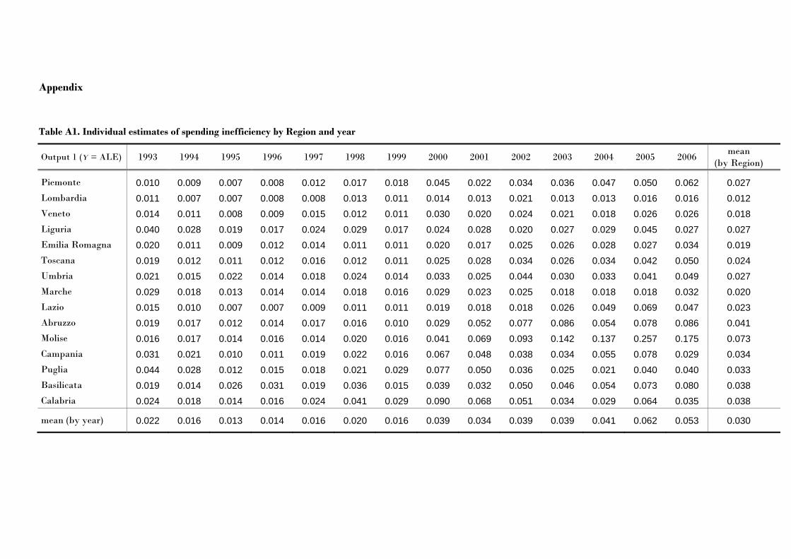
Appendix

Table A1. Individual estimates of spending inefficiency by Region and year

Output 1 (Y = ALE) 1993 1994 1995 1996 1997 1998 1999 2000 2001 2002 2003 2004 2005 2006 mean

(by Region)

Piemonte 0.010 0.009 0.007 0.008 0.012 0.017 0.018 0.045 0.022 0.034 0.036 0.047 0.050 0.062 0.027 Lombardia 0.011 0.007 0.007 0.008 0.008 0.013 0.011 0.014 0.013 0.021 0.013 0.013 0.016 0.016 0.012 Veneto 0.014 0.011 0.008 0.009 0.015 0.012 0.011 0.030 0.020 0.024 0.021 0.018 0.026 0.026 0.018 Liguria 0.040 0.028 0.019 0.017 0.024 0.029 0.017 0.024 0.028 0.020 0.027 0.029 0.045 0.027 0.027 Emilia Romagna 0.020 0.011 0.009 0.012 0.014 0.011 0.011 0.020 0.017 0.025 0.026 0.028 0.027 0.034 0.019 Toscana 0.019 0.012 0.011 0.012 0.016 0.012 0.011 0.025 0.028 0.034 0.026 0.034 0.042 0.050 0.024 Umbria 0.021 0.015 0.022 0.014 0.018 0.024 0.014 0.033 0.025 0.044 0.030 0.033 0.041 0.049 0.027 Marche 0.029 0.018 0.013 0.014 0.014 0.018 0.016 0.029 0.023 0.025 0.018 0.018 0.018 0.032 0.020 Lazio 0.015 0.010 0.007 0.007 0.009 0.011 0.011 0.019 0.018 0.018 0.026 0.049 0.069 0.047 0.023 Abruzzo 0.019 0.017 0.012 0.014 0.017 0.016 0.010 0.029 0.052 0.077 0.086 0.054 0.078 0.086 0.041 Molise 0.016 0.017 0.014 0.016 0.014 0.020 0.016 0.041 0.069 0.093 0.142 0.137 0.257 0.175 0.073 Campania 0.031 0.021 0.010 0.011 0.019 0.022 0.016 0.067 0.048 0.038 0.034 0.055 0.078 0.029 0.034 Puglia 0.044 0.028 0.012 0.015 0.018 0.021 0.029 0.077 0.050 0.036 0.025 0.021 0.040 0.040 0.033 Basilicata 0.019 0.014 0.026 0.031 0.019 0.036 0.015 0.039 0.032 0.050 0.046 0.054 0.073 0.080 0.038 Calabria 0.024 0.018 0.014 0.016 0.024 0.041 0.029 0.090 0.068 0.051 0.034 0.029 0.064 0.035 0.038

mean (by year) 0.022 0.016 0.013 0.014 0.016 0.020 0.016 0.039 0.034 0.039 0.039 0.041 0.062 0.053 0.030

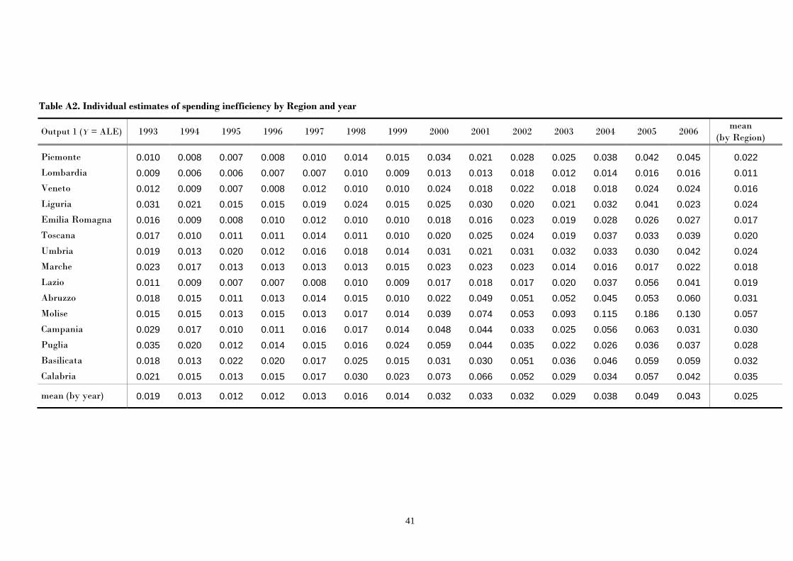
41

Table A2. Individual estimates of spending inefficiency by Region and year

Output 1 (Y = ALE) 1993 1994 1995 1996 1997 1998 1999 2000 2001 2002 2003 2004 2005 2006 mean

(by Region)

Piemonte 0.010 0.008 0.007 0.008 0.010 0.014 0.015 0.034 0.021 0.028 0.025 0.038 0.042 0.045 0.022 Lombardia 0.009 0.006 0.006 0.007 0.007 0.010 0.009 0.013 0.013 0.018 0.012 0.014 0.016 0.016 0.011 Veneto 0.012 0.009 0.007 0.008 0.012 0.010 0.010 0.024 0.018 0.022 0.018 0.018 0.024 0.024 0.016 Liguria 0.031 0.021 0.015 0.015 0.019 0.024 0.015 0.025 0.030 0.020 0.021 0.032 0.041 0.023 0.024 Emilia Romagna 0.016 0.009 0.008 0.010 0.012 0.010 0.010 0.018 0.016 0.023 0.019 0.028 0.026 0.027 0.017 Toscana 0.017 0.010 0.011 0.011 0.014 0.011 0.010 0.020 0.025 0.024 0.019 0.037 0.033 0.039 0.020 Umbria 0.019 0.013 0.020 0.012 0.016 0.018 0.014 0.031 0.021 0.031 0.032 0.033 0.030 0.042 0.024 Marche 0.023 0.017 0.013 0.013 0.013 0.013 0.015 0.023 0.023 0.023 0.014 0.016 0.017 0.022 0.018 Lazio 0.011 0.009 0.007 0.007 0.008 0.010 0.009 0.017 0.018 0.017 0.020 0.037 0.056 0.041 0.019 Abruzzo 0.018 0.015 0.011 0.013 0.014 0.015 0.010 0.022 0.049 0.051 0.052 0.045 0.053 0.060 0.031 Molise 0.015 0.015 0.013 0.015 0.013 0.017 0.014 0.039 0.074 0.053 0.093 0.115 0.186 0.130 0.057 Campania 0.029 0.017 0.010 0.011 0.016 0.017 0.014 0.048 0.044 0.033 0.025 0.056 0.063 0.031 0.030 Puglia 0.035 0.020 0.012 0.014 0.015 0.016 0.024 0.059 0.044 0.035 0.022 0.026 0.036 0.037 0.028 Basilicata 0.018 0.013 0.022 0.020 0.017 0.025 0.015 0.031 0.030 0.051 0.036 0.046 0.059 0.059 0.032 Calabria 0.021 0.015 0.013 0.015 0.017 0.030 0.023 0.073 0.066 0.052 0.029 0.034 0.057 0.042 0.035

mean (by year) 0.019 0.013 0.012 0.012 0.013 0.016 0.014 0.032 0.033 0.032 0.029 0.038 0.049 0.043 0.025

DEPARTMENT OF ECONOMICS AND PUBLIC FINANCE “G. PRATO”

UNIVERSITY OF TORINO Corso Unione Sovietica 218 bis - 10134 Torino (ITALY)

Phone: +39 011 6706128 - Fax: +39 011 6706062 Web page: http://eco83.econ.unito.it/prato/