Embed Size (px)
Citation preview

How far can we go with Lieb’s concavitytheorem and Ando’s convexity theorem?
Haonan Zhang (IST Austria)
Based on arXiv:1811.01205, Adv. Math. 2020.
Entropy Inequalities, Quantum Information and Quantum PhysicsIPAM, February 08 -11, 2021
0/37

1/37
Stability of concavity
The concavity of trace functionals is stable underI linear combinations with positive coefficients;I limits;I inf;I sup with additional conditions;I ...
Given the concavity/convexity of certain functionals (Lieb, Ando), onecan derive the concavity/convexity of more functionals, e.g. thosewith nice integral formula. We will see that inf/sup can be very useful.
2/37
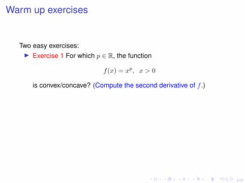
Warm up exercises
Two easy exercises:I Exercise 1 For which p ∈ R, the function
f(x) = xp, x > 0
is convex/concave? (Compute the second derivative of f .)
For a two-variable function, one can ask the joint convexity/concavity:I Exercise 2 For which (p, q) ∈ R2, the function
f(x, y) = xpyq, x, y > 0
is jointly convex/concave? (Compute the Hessian of f .)
2/37
Warm up exercises
Two easy exercises:I Exercise 1 For which p ∈ R, the function
f(x) = xp, x > 0
is convex/concave? (Compute the second derivative of f .)For a two-variable function, one can ask the joint convexity/concavity:I Exercise 2 For which (p, q) ∈ R2, the function
f(x, y) = xpyq, x, y > 0
is jointly convex/concave? (Compute the Hessian of f .)
3/37
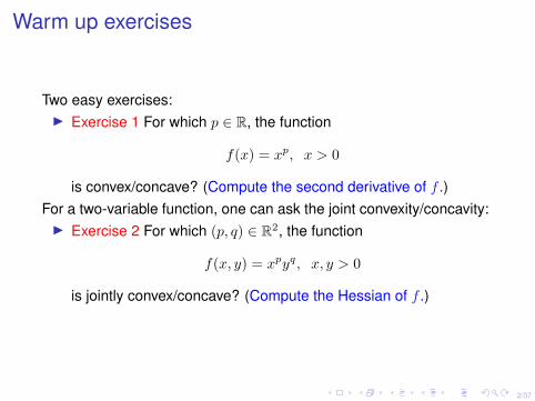
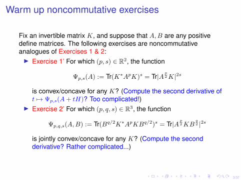
Warm up noncommutative exercises
Fix an invertible matrix K, and suppose that A,B are any positivedefine matrices. The following exercises are noncommutativeanalogues of Exercises 1 & 2:I Exercise 1’ For which (p, s) ∈ R2, the function
Ψp,s(A) := Tr(K∗ApK)s = Tr|Ap2K|2s
is convex/concave for any K? (Compute the second derivative oft 7→ Ψp,s(A+ tH)? Too complicated!)
I Exercise 2’ For which (p, q, s) ∈ R3, the function
Ψp,q,s(A,B) := Tr(Bq/2K∗ApKBq/2)s = Tr|Ap2KB
q2 |2s
is jointly convex/concave for any K? (Compute the secondderivative? Rather complicated...)
3/37
Warm up noncommutative exercises
Fix an invertible matrix K, and suppose that A,B are any positivedefine matrices. The following exercises are noncommutativeanalogues of Exercises 1 & 2:I Exercise 1’ For which (p, s) ∈ R2, the function
Ψp,s(A) := Tr(K∗ApK)s = Tr|Ap2K|2s
is convex/concave for any K? (Compute the second derivative oft 7→ Ψp,s(A+ tH)? Too complicated!)
I Exercise 2’ For which (p, q, s) ∈ R3, the function
Ψp,q,s(A,B) := Tr(Bq/2K∗ApKBq/2)s = Tr|Ap2KB
q2 |2s
is jointly convex/concave for any K? (Compute the secondderivative? Rather complicated...)
4/37
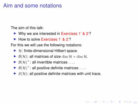
Aim and some notations
The aim of this talk:I Why we are interested in Exercises 1’ & 2’?I How to solve Exercises 1’ & 2’?
For this we will use the following notations:I H: finite-dimensional Hilbert space.I B(H): all matrices of size dimH× dimH.I B(H)
×: all invertible matrices . . . .I B(H)
+: all positive definite matrices . . . .I S(H): all positive definite matrices with unit trace.
4/37
Aim and some notations
The aim of this talk:I Why we are interested in Exercises 1’ & 2’?I How to solve Exercises 1’ & 2’?
For this we will use the following notations:I H: finite-dimensional Hilbert space.I B(H): all matrices of size dimH× dimH.I B(H)
×: all invertible matrices . . . .I B(H)
+: all positive definite matrices . . . .I S(H): all positive definite matrices with unit trace.
5/37
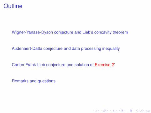
Outline
Wigner-Yanase-Dyson conjecture and Lieb’s concavity theorem
Audenaert-Datta conjecture and data processing inequality
Carlen-Frank-Lieb conjecture and solution of Exercise 2’
Remarks and questions
6/37
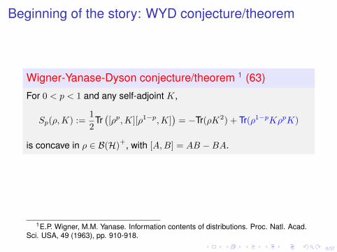
Beginning of the story: WYD conjecture/theorem
Wigner-Yanase-Dyson conjecture/theorem 1 (63)
For 0 < p < 1 and any self-adjoint K,
Sp(ρ,K) :=1
2Tr([ρp,K][ρ1−p,K]
)= −Tr(ρK2) + Tr(ρ1−pKρpK)
is concave in ρ ∈ B(H)+, with [A,B] = AB −BA.
1E.P. Wigner, M.M. Yanase. Information contents of distributions. Proc. Natl. Acad.Sci. USA, 49 (1963), pp. 910-918.
7/37
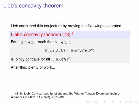
Lieb’s concavity theorem
Lieb confirmed this conjecture by proving the following celebrated
Lieb’s concavity theorem (73) 2
For 0 ≤ p, q ≤ 1 such that p+ q ≤ 1,
Ψp,q,1(A,B) = Tr(K∗ApKBq)
is jointly concave for all K ∈ B(H)×.
After this: plenty of work...
2E. H. Lieb. Convex trace functions and the Wigner-Yanase-Dyson conjecture.Advances in Math. 11 (1973), 267–288.
8/37
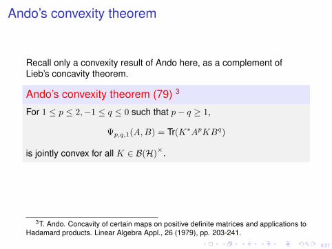
Ando’s convexity theorem
Recall only a convexity result of Ando here, as a complement ofLieb’s concavity theorem.
Ando’s convexity theorem (79) 3
For 1 ≤ p ≤ 2,−1 ≤ q ≤ 0 such that p− q ≥ 1,
Ψp,q,1(A,B) = Tr(K∗ApKBq)
is jointly convex for all K ∈ B(H)×.
3T. Ando. Concavity of certain maps on positive definite matrices and applications toHadamard products. Linear Algebra Appl., 26 (1979), pp. 203-241.

9/37
Wigner-Yanase-Dyson conjecture and Lieb’s concavity theorem
Audenaert-Datta conjecture and data processing inequality
Carlen-Frank-Lieb conjecture and solution of Exercise 2’
Remarks and questions
10/37
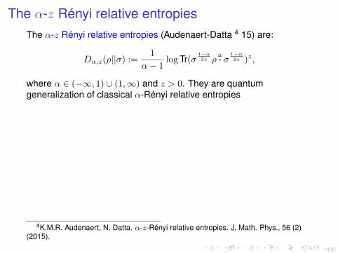
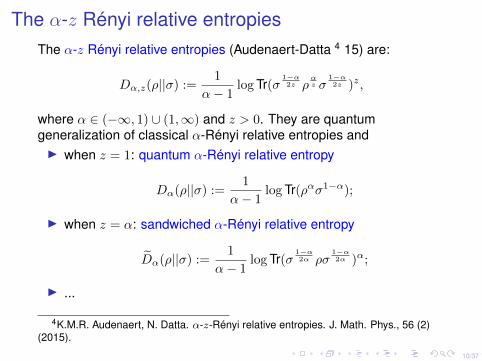
The α-z Rényi relative entropiesThe α-z Rényi relative entropies (Audenaert-Datta 4 15) are:
Dα,z(ρ||σ) :=1
α− 1log Tr(σ
1−α2z ρ
αz σ
1−α2z )z,
where α ∈ (−∞, 1) ∪ (1,∞) and z > 0. They are quantumgeneralization of classical α-Rényi relative entropies
andI when z = 1: quantum α-Rényi relative entropy
Dα(ρ||σ) :=1
α− 1log Tr(ρασ1−α);
I when z = α: sandwiched α-Rényi relative entropy
D̃α(ρ||σ) :=1
α− 1log Tr(σ
1−α2α ρσ
1−α2α )α;
I ...
4K.M.R. Audenaert, N. Datta. α-z-Rényi relative entropies. J. Math. Phys., 56 (2)(2015).
10/37
The α-z Rényi relative entropiesThe α-z Rényi relative entropies (Audenaert-Datta 4 15) are:
Dα,z(ρ||σ) :=1
α− 1log Tr(σ
1−α2z ρ
αz σ
1−α2z )z,
where α ∈ (−∞, 1) ∪ (1,∞) and z > 0. They are quantumgeneralization of classical α-Rényi relative entropies andI when z = 1: quantum α-Rényi relative entropy
Dα(ρ||σ) :=1
α− 1log Tr(ρασ1−α);
I when z = α: sandwiched α-Rényi relative entropy
D̃α(ρ||σ) :=1
α− 1log Tr(σ
1−α2α ρσ
1−α2α )α;
I ...
4K.M.R. Audenaert, N. Datta. α-z-Rényi relative entropies. J. Math. Phys., 56 (2)(2015).

11/37
12/37
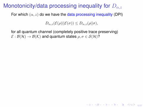
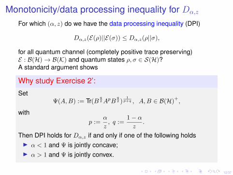
Monotonicity/data processing inequality for Dα,z
For which (α, z) do we have the data processing inequality (DPI)
Dα,z(E(ρ)||E(σ)) ≤ Dα,z(ρ||σ),
for all quantum channel (completely positive trace preserving)E : B(H)→ B(K) and quantum states ρ, σ ∈ S(H)?
A standard argument shows
Why study Exercise 2’:
SetΨ(A,B) := Tr(B
q2ApB
q2 )
1p+q , A,B ∈ B(H)
+,
withp :=
α
z, q :=
1− αz
.
Then DPI holds for Dα,z if and only if one of the following holdsI α < 1 and Ψ is jointly concave;I α > 1 and Ψ is jointly convex.
12/37
Monotonicity/data processing inequality for Dα,z
For which (α, z) do we have the data processing inequality (DPI)
Dα,z(E(ρ)||E(σ)) ≤ Dα,z(ρ||σ),
for all quantum channel (completely positive trace preserving)E : B(H)→ B(K) and quantum states ρ, σ ∈ S(H)?A standard argument shows
Why study Exercise 2’:
SetΨ(A,B) := Tr(B
q2ApB
q2 )
1p+q , A,B ∈ B(H)
+,
withp :=
α
z, q :=
1− αz
.
Then DPI holds for Dα,z if and only if one of the following holdsI α < 1 and Ψ is jointly concave;I α > 1 and Ψ is jointly convex.
13/37
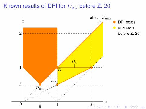
Known results of DPI for Dα,z before Z. 20
α
z
0 12
1 2
12
1
2
Dmin
D
Dα
D̃α
at∞ : Dmax
DPI holdsunknownbefore Z. 20
AD conjecture
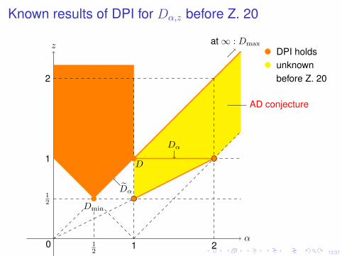
13/37
Known results of DPI for Dα,z before Z. 20
α
z
0 12
1 2
12
1
2
Dmin
D
Dα
D̃α
at∞ : Dmax
DPI holdsunknownbefore Z. 20
AD conjecture
14/37
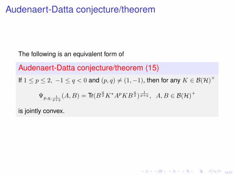
Audenaert-Datta conjecture/theorem
The following is an equivalent form of
Audenaert-Datta conjecture/theorem (15)
If 1 ≤ p ≤ 2, −1 ≤ q < 0 and (p, q) 6= (1,−1), then for any K ∈ B(H)×
Ψp,q, 1p+q
(A,B) = Tr(Bq2K∗ApKB
q2 )
1p+q , A,B ∈ B(H)
+
is jointly convex.
15/37
Wigner-Yanase-Dyson conjecture and Lieb’s concavity theorem
Audenaert-Datta conjecture and data processing inequality
Carlen-Frank-Lieb conjecture and solution of Exercise 2’
Remarks and questions
16/37
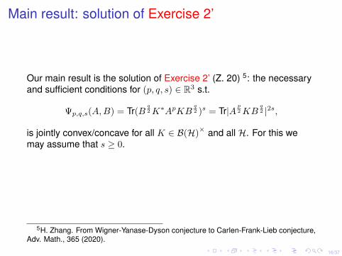
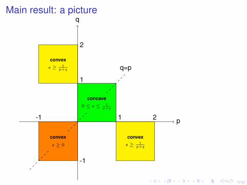
Main result: solution of Exercise 2’
Our main result is the solution of Exercise 2’ (Z. 20) 5: the necessaryand sufficient conditions for (p, q, s) ∈ R3 s.t.
Ψp,q,s(A,B) = Tr(Bq2K∗ApKB
q2 )s = Tr|A
p2KB
q2 |2s,
is jointly convex/concave for all K ∈ B(H)× and all H. For this we
may assume that s ≥ 0.
5H. Zhang. From Wigner-Yanase-Dyson conjecture to Carlen-Frank-Lieb conjecture,Adv. Math., 365 (2020).
17/37
Main result: a picture
o
concave0 ≤ s ≤ 1
p+q
convexs ≥ 1
p+q
convex
s ≥ 0
convexs ≥ 1
p+q
-1
-1
1 2
1
2
q=p
p
q

18/37
Brief history
It takes a long time to complete this picture. Hiai 6 (13) proved thatthese conditions are necessary by testing 4-by-4 matrices. The firstsignificant sufficient result is the Lieb’s concavity theorem. We willcomplete the whole “sufficient” picture using the following buildingblocks:
6F. Hiai. Concavity of certain matrix trace and norm functions. Linear Algebra Appl.,439 (5) (2013), pp. 1568-1589.
19/37
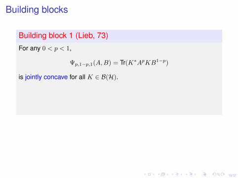
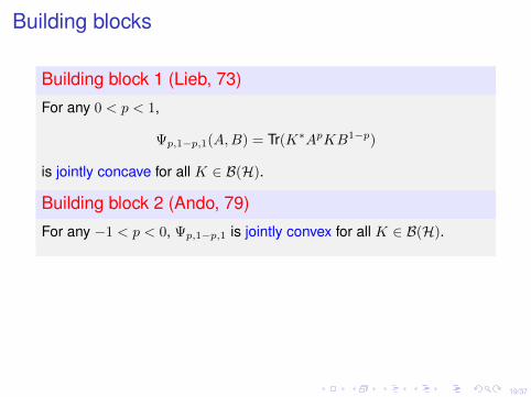
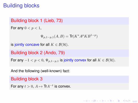
Building blocks
Building block 1 (Lieb, 73)
For any 0 < p < 1,
Ψp,1−p,1(A,B) = Tr(K∗ApKB1−p)
is jointly concave for all K ∈ B(H).
Building block 2 (Ando, 79)
For any −1 < p < 0, Ψp,1−p,1 is jointly convex for all K ∈ B(H).
And the following (well-known) fact:
Building block 3
For any t > 0, A 7→ TrA−t is convex.
19/37
Building blocks
Building block 1 (Lieb, 73)
For any 0 < p < 1,
Ψp,1−p,1(A,B) = Tr(K∗ApKB1−p)
is jointly concave for all K ∈ B(H).
Building block 2 (Ando, 79)
For any −1 < p < 0, Ψp,1−p,1 is jointly convex for all K ∈ B(H).
And the following (well-known) fact:
Building block 3
For any t > 0, A 7→ TrA−t is convex.
20/37
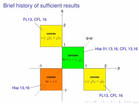
Brief history of sufficient results
p
q
o
concavefor 0 ≤ s ≤ 1
p+q
convexs ≥ 1
p−1 ∧1q+1
convex
for s ≥ 0
convexs ≥ 1
p+1 ∧1q−1
-1
-1
1 2
1
2
q=p
Hiai 01,13,16, CFL 13,16
Hiai 13,16
FL13, CFL 16
FL13, CFL 16
CFL conjecture:convex for s ≥ 1
p+q

20/37
Brief history of sufficient results
p
q
o
concavefor 0 ≤ s ≤ 1
p+q
convexs ≥ 1
p−1 ∧1q+1
convex
for s ≥ 0
convexs ≥ 1
p+1 ∧1q−1
-1
-1
1 2
1
2
q=p
Hiai 01,13,16, CFL 13,16
Hiai 13,16
FL13, CFL 16
FL13, CFL 16CFL conjecture:
convex for s ≥ 1p+q
21/37
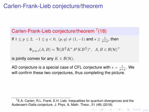
Carlen-Frank-Lieb conjecture/theorem
Carlen-Frank-Lieb conjecture/theorem 7(18)
If 1 ≤ p ≤ 2, −1 ≤ q < 0, (p, q) 6= (1,−1) and s ≥ 1p+q , then
Ψp,q,s(A,B) = Tr(Bq2K∗ApKB
q2 )s, A,B ∈ B(H)
+
is jointly convex for any K ∈ B(H).
AD conjecture is a special case of CFL conjecture with s = 1p+q . We
will confirm these two conjectures, thus completing the picture.
7E.A. Carlen, R.L. Frank, E.H. Lieb. Inequalities for quantum divergences and theAudenaert–Datta conjecture. J. Phys. A, Math. Theor., 51 (48) (2018).
22/37
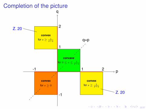
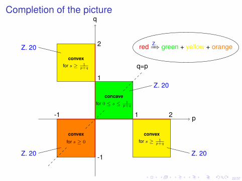
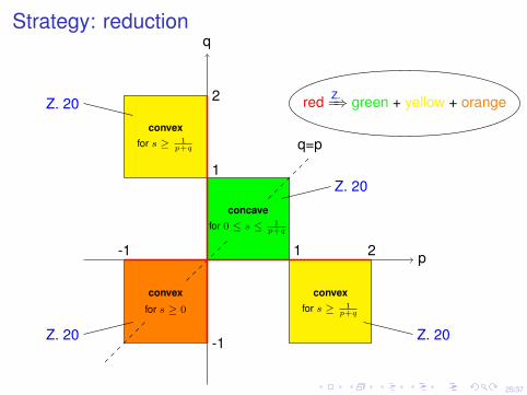
Completion of the picture
o
concavefor 0 ≤ s ≤ 1
p+q
convexfor s ≥ 1
p+q
convex
for s ≥ 0
convexfor s ≥ 1
p+q
-1
-1
1 2
1
2
q=p
p
q
Z. 20
Z. 20
Z. 20
Z. 20
red Z.=⇒ green + yellow + orange

22/37
Completion of the picture
o
concavefor 0 ≤ s ≤ 1
p+q
convexfor s ≥ 1
p+q
convex
for s ≥ 0
convexfor s ≥ 1
p+q
-1
-1
1 2
1
2
q=p
p
q
Z. 20
Z. 20
Z. 20
Z. 20
red Z.=⇒ green + yellow + orange
22/37
Completion of the picture
o
concavefor 0 ≤ s ≤ 1
p+q
convexfor s ≥ 1
p+q
convex
for s ≥ 0
convexfor s ≥ 1
p+q
-1
-1
1 2
1
2
q=p
p
q
Z. 20
Z. 20
Z. 20
Z. 20
red Z.=⇒ green + yellow + orange
23/37
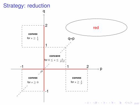
Strategy: reduction
o
concavefor 0 ≤ s ≤ 1
p(q)
convexfor s ≥ 1
p
convex
for s ≥ 0
convexfor s ≥ 1
q
-1
-1
1 2
1
2
q=p
p
q
red
24/37
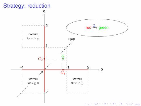
Strategy: reduction
o
convexfor s ≥ 1
p
convex
for s ≥ 0
convexfor s ≥ 1
q
-1
-1
1 2
1
2
q=p
p
q
red Z.=⇒ green
GG2
G1
25/37
Strategy: reduction
o
concavefor 0 ≤ s ≤ 1
p+q
convexfor s ≥ 1
p+q
convex
for s ≥ 0
convexfor s ≥ 1
p+q
-1
-1
1 2
1
2
q=p
p
q
Z. 20
Z. 20
Z. 20
Z. 20
red Z.=⇒ green + yellow + orange
26/37
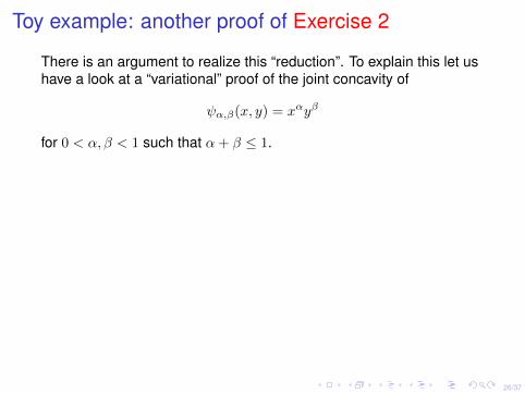
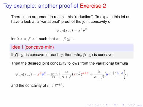
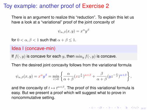
Toy example: another proof of Exercise 2
There is an argument to realize this “reduction”. To explain this let ushave a look at a “variational” proof of the joint concavity of
ψα,β(x, y) = xαyβ
for 0 < α, β < 1 such that α+ β ≤ 1.
Idea I (concave-min)
If f(·, y) is concave for each y, then miny f(·, y) is concave.
Then the desired joint concavity follows from the variational formula
ψα,β(x, y) = xαyβ = minz>0
{α
α+ β(xz
1α )α+β +
β
α+ β(yz−
1β )α+β
},
and the concavity of t 7→ tα+β . The proof of this variational formula iseasy. But we present a proof which will suggest what to prove innoncommutative setting.
26/37
Toy example: another proof of Exercise 2
There is an argument to realize this “reduction”. To explain this let ushave a look at a “variational” proof of the joint concavity of
ψα,β(x, y) = xαyβ
for 0 < α, β < 1 such that α+ β ≤ 1.
Idea I (concave-min)
If f(·, y) is concave for each y, then miny f(·, y) is concave.
Then the desired joint concavity follows from the variational formula
ψα,β(x, y) = xαyβ = minz>0
{α
α+ β(xz
1α )α+β +
β
α+ β(yz−
1β )α+β
},
and the concavity of t 7→ tα+β .
The proof of this variational formula iseasy. But we present a proof which will suggest what to prove innoncommutative setting.
26/37
Toy example: another proof of Exercise 2
There is an argument to realize this “reduction”. To explain this let ushave a look at a “variational” proof of the joint concavity of
ψα,β(x, y) = xαyβ
for 0 < α, β < 1 such that α+ β ≤ 1.
Idea I (concave-min)
If f(·, y) is concave for each y, then miny f(·, y) is concave.
Then the desired joint concavity follows from the variational formula
ψα,β(x, y) = xαyβ = minz>0
{α
α+ β(xz
1α )α+β +
β
α+ β(yz−
1β )α+β
},
and the concavity of t 7→ tα+β . The proof of this variational formula iseasy. But we present a proof which will suggest what to prove innoncommutative setting.
27/37
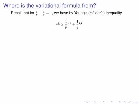
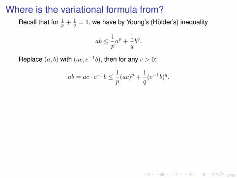
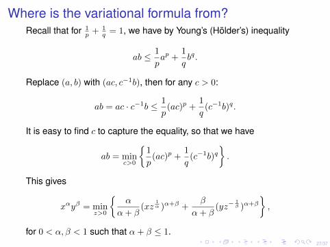
Where is the variational formula from?Recall that for 1
p + 1q = 1, we have by Young’s (Hölder’s) inequality
ab ≤ 1
pap +
1
qbq.
Replace (a, b) with (ac, c−1b), then for any c > 0:
ab = ac · c−1b ≤ 1
p(ac)p +
1
q(c−1b)q.
It is easy to find c to capture the equality, so that we have
ab = minc>0
{1
p(ac)p +
1
q(c−1b)q
}.
This gives
xαyβ = minz>0
{α
α+ β(xz
1α )α+β +
β
α+ β(yz−
1β )α+β
},
for 0 < α, β < 1 such that α+ β ≤ 1.
27/37
Where is the variational formula from?Recall that for 1
p + 1q = 1, we have by Young’s (Hölder’s) inequality
ab ≤ 1
pap +
1
qbq.
Replace (a, b) with (ac, c−1b), then for any c > 0:
ab = ac · c−1b ≤ 1
p(ac)p +
1
q(c−1b)q.
It is easy to find c to capture the equality, so that we have
ab = minc>0
{1
p(ac)p +
1
q(c−1b)q
}.
This gives
xαyβ = minz>0
{α
α+ β(xz
1α )α+β +
β
α+ β(yz−
1β )α+β
},
for 0 < α, β < 1 such that α+ β ≤ 1.
28/37
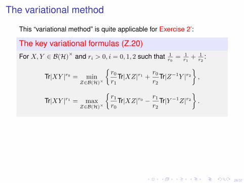
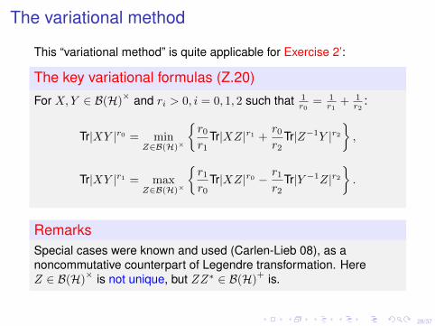
The variational method
This “variational method” is quite applicable for Exercise 2’:
The key variational formulas (Z.20)
For X,Y ∈ B(H)× and ri > 0, i = 0, 1, 2 such that 1
r0= 1
r1+ 1
r2:
Tr|XY |r0 = minZ∈B(H)×
{r0r1
Tr|XZ|r1 +r0r2
Tr|Z−1Y |r2},
Tr|XY |r1 = maxZ∈B(H)×
{r1r0
Tr|XZ|r0 − r1r2
Tr|Y −1Z|r2}.
RemarksSpecial cases were known and used (Carlen-Lieb 08), as anoncommutative counterpart of Legendre transformation. HereZ ∈ B(H)
× is not unique, but ZZ∗ ∈ B(H)+ is.
28/37
The variational method
This “variational method” is quite applicable for Exercise 2’:
The key variational formulas (Z.20)
For X,Y ∈ B(H)× and ri > 0, i = 0, 1, 2 such that 1
r0= 1
r1+ 1
r2:
Tr|XY |r0 = minZ∈B(H)×
{r0r1
Tr|XZ|r1 +r0r2
Tr|Z−1Y |r2},
Tr|XY |r1 = maxZ∈B(H)×
{r1r0
Tr|XZ|r0 − r1r2
Tr|Y −1Z|r2}.
RemarksSpecial cases were known and used (Carlen-Lieb 08), as anoncommutative counterpart of Legendre transformation. HereZ ∈ B(H)
× is not unique, but ZZ∗ ∈ B(H)+ is.
29/37
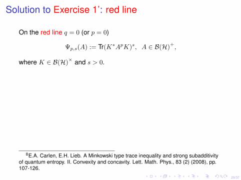
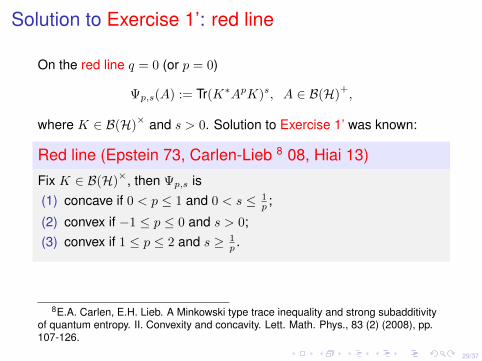
Solution to Exercise 1’: red line
On the red line q = 0 (or p = 0)
Ψp,s(A) := Tr(K∗ApK)s, A ∈ B(H)+,
where K ∈ B(H)× and s > 0.
Solution to Exercise 1’ was known:
Red line (Epstein 73, Carlen-Lieb 8 08, Hiai 13)
Fix K ∈ B(H)×, then Ψp,s is
(1) concave if 0 < p ≤ 1 and 0 < s ≤ 1p ;
(2) convex if −1 ≤ p ≤ 0 and s > 0;(3) convex if 1 ≤ p ≤ 2 and s ≥ 1
p .
8E.A. Carlen, E.H. Lieb. A Minkowski type trace inequality and strong subadditivityof quantum entropy. II. Convexity and concavity. Lett. Math. Phys., 83 (2) (2008), pp.107-126.
29/37
Solution to Exercise 1’: red line
On the red line q = 0 (or p = 0)
Ψp,s(A) := Tr(K∗ApK)s, A ∈ B(H)+,
where K ∈ B(H)× and s > 0. Solution to Exercise 1’ was known:
Red line (Epstein 73, Carlen-Lieb 8 08, Hiai 13)
Fix K ∈ B(H)×, then Ψp,s is
(1) concave if 0 < p ≤ 1 and 0 < s ≤ 1p ;
(2) convex if −1 ≤ p ≤ 0 and s > 0;(3) convex if 1 ≤ p ≤ 2 and s ≥ 1
p .
8E.A. Carlen, E.H. Lieb. A Minkowski type trace inequality and strong subadditivityof quantum entropy. II. Convexity and concavity. Lett. Math. Phys., 83 (2) (2008), pp.107-126.
30/37
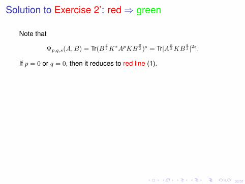
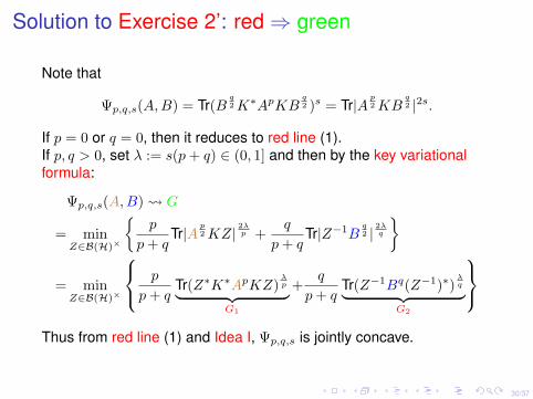
Solution to Exercise 2’: red⇒ green
Note that
Ψp,q,s(A,B) = Tr(Bq2K∗ApKB
q2 )s = Tr|A
p2KB
q2 |2s.
If p = 0 or q = 0, then it reduces to red line (1).
If p, q > 0, set λ := s(p+ q) ∈ (0, 1] and then by the key variationalformula:
Ψp,q,s(A,B) G
= minZ∈B(H)×
{p
p+ qTr|A
p2KZ|
2λp +
q
p+ qTr|Z−1B
q2 |
2λq
}
= minZ∈B(H)×
p
p+ qTr(Z∗K∗ApKZ)
λp︸ ︷︷ ︸
G1
+q
p+ qTr(Z−1Bq(Z−1)∗)
λq︸ ︷︷ ︸
G2
Thus from red line (1) and Idea I, Ψp,q,s is jointly concave.
30/37
Solution to Exercise 2’: red⇒ green
Note that
Ψp,q,s(A,B) = Tr(Bq2K∗ApKB
q2 )s = Tr|A
p2KB
q2 |2s.
If p = 0 or q = 0, then it reduces to red line (1).If p, q > 0, set λ := s(p+ q) ∈ (0, 1] and then by the key variationalformula:
Ψp,q,s(A,B) G
= minZ∈B(H)×
{p
p+ qTr|A
p2KZ|
2λp +
q
p+ qTr|Z−1B
q2 |
2λq
}
= minZ∈B(H)×
p
p+ qTr(Z∗K∗ApKZ)
λp︸ ︷︷ ︸
G1
+q
p+ qTr(Z−1Bq(Z−1)∗)
λq︸ ︷︷ ︸
G2
Thus from red line (1) and Idea I, Ψp,q,s is jointly concave.
31/37
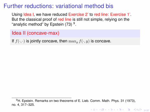
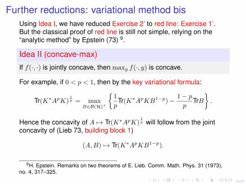
Further reductions: variational method bisUsing Idea I, we have reduced Exercise 2’ to red line: Exercise 1’.But the classical proof of red line is still not simple, relying on the“analytic method” by Epstein (73) 9.
Idea II (concave-max)
If f(·, ·) is jointly concave, then maxy f(·, y) is concave.
For example, if 0 < p < 1, then by the key variational formula:
Tr(K∗ApK)1p = max
B∈B(H)+
{1
pTr(K∗ApKB1−p)− 1− p
pTrB
}.
Hence the concavity of A 7→ Tr(K∗ApK)1p will follow from the joint
concavity of (Lieb 73, building block 1)
(A,B) 7→ Tr(K∗ApKB1−p).
9H. Epstein. Remarks on two theorems of E. Lieb. Comm. Math. Phys. 31 (1973),no. 4, 317–325.
31/37
Further reductions: variational method bisUsing Idea I, we have reduced Exercise 2’ to red line: Exercise 1’.But the classical proof of red line is still not simple, relying on the“analytic method” by Epstein (73) 9.
Idea II (concave-max)
If f(·, ·) is jointly concave, then maxy f(·, y) is concave.
For example, if 0 < p < 1, then by the key variational formula:
Tr(K∗ApK)1p = max
B∈B(H)+
{1
pTr(K∗ApKB1−p)− 1− p
pTrB
}.
Hence the concavity of A 7→ Tr(K∗ApK)1p will follow from the joint
concavity of (Lieb 73, building block 1)
(A,B) 7→ Tr(K∗ApKB1−p).
9H. Epstein. Remarks on two theorems of E. Lieb. Comm. Math. Phys. 31 (1973),no. 4, 317–325.

32/37
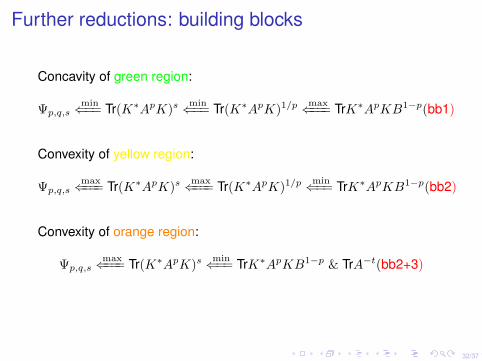
Further reductions: building blocks
Concavity of green region:
Ψp,q,smin⇐== Tr(K∗ApK)s
min⇐== Tr(K∗ApK)1/pmax⇐=== TrK∗ApKB1−p(bb1)
Convexity of yellow region:
Ψp,q,smax⇐=== Tr(K∗ApK)s
max⇐=== Tr(K∗ApK)1/pmin⇐== TrK∗ApKB1−p(bb2)
Convexity of orange region:
Ψp,q,smax⇐=== Tr(K∗ApK)s
min⇐== TrK∗ApKB1−p & TrA−t(bb2+3)
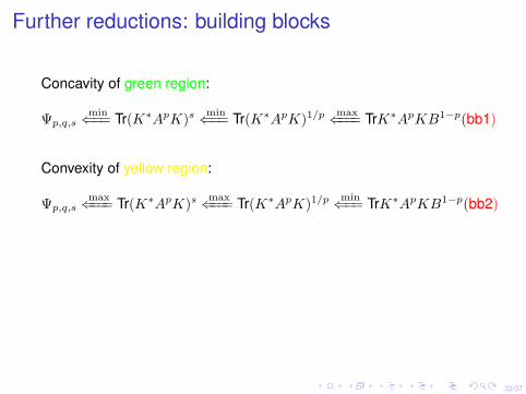
32/37
Further reductions: building blocks
Concavity of green region:
Ψp,q,smin⇐== Tr(K∗ApK)s
min⇐== Tr(K∗ApK)1/pmax⇐=== TrK∗ApKB1−p(bb1)
Convexity of yellow region:
Ψp,q,smax⇐=== Tr(K∗ApK)s
max⇐=== Tr(K∗ApK)1/pmin⇐== TrK∗ApKB1−p(bb2)
Convexity of orange region:
Ψp,q,smax⇐=== Tr(K∗ApK)s
min⇐== TrK∗ApKB1−p & TrA−t(bb2+3)
33/37
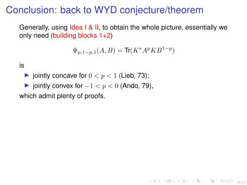
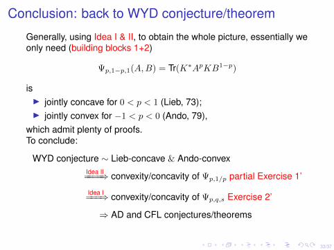
Conclusion: back to WYD conjecture/theorem
Generally, using Idea I & II, to obtain the whole picture, essentially weonly need (building blocks 1+2)
Ψp,1−p,1(A,B) = Tr(K∗ApKB1−p)
isI jointly concave for 0 < p < 1 (Lieb, 73);I jointly convex for −1 < p < 0 (Ando, 79),
which admit plenty of proofs.
To conclude:
WYD conjecture ∼ Lieb-concave & Ando-convexIdea II====⇒ convexity/concavity of Ψp,1/p partial Exercise 1’
Idea I===⇒ convexity/concavity of Ψp,q,s Exercise 2’
⇒ AD and CFL conjectures/theorems
33/37
Conclusion: back to WYD conjecture/theorem
Generally, using Idea I & II, to obtain the whole picture, essentially weonly need (building blocks 1+2)
Ψp,1−p,1(A,B) = Tr(K∗ApKB1−p)
isI jointly concave for 0 < p < 1 (Lieb, 73);I jointly convex for −1 < p < 0 (Ando, 79),
which admit plenty of proofs.To conclude:
WYD conjecture ∼ Lieb-concave & Ando-convexIdea II====⇒ convexity/concavity of Ψp,1/p partial Exercise 1’
Idea I===⇒ convexity/concavity of Ψp,q,s Exercise 2’
⇒ AD and CFL conjectures/theorems

34/37
Wigner-Yanase-Dyson conjecture and Lieb’s concavity theorem
Audenaert-Datta conjecture and data processing inequality
Carlen-Frank-Lieb conjecture and solution of Exercise 2’
Remarks and questions
35/37
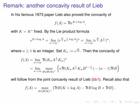
Remark: another concavity result of LiebIn his famous 1973 paper Lieb also proved the concavity of
f(A) = TreK+logA,
with K = K∗ fixed.
By the Lie product formula
eK+logA = limn→∞
(eKn e
1n logA)n = lim
n→∞(e
Kn A
1n )n,
where n ≥ 1 is an integer. Set Kn := eK2n . Then the concavity of
f(A) = limn→∞
Tr(KnA1nKn)n
= limn→∞
maxB∈B(H)+
{nTr(KnA
1nKnB
1− 1n )− (n− 1)TrB
}will follow from the joint concavity result of Lieb (bb1). Recall also that
f(A) = maxB∈B(H)+
{TrB(K + logA)− TrB logB + TrB} .
35/37
Remark: another concavity result of LiebIn his famous 1973 paper Lieb also proved the concavity of
f(A) = TreK+logA,
with K = K∗ fixed. By the Lie product formula
eK+logA = limn→∞
(eKn e
1n logA)n = lim
n→∞(e
Kn A
1n )n,
where n ≥ 1 is an integer. Set Kn := eK2n . Then the concavity of
f(A) = limn→∞
Tr(KnA1nKn)n
= limn→∞
maxB∈B(H)+
{nTr(KnA
1nKnB
1− 1n )− (n− 1)TrB
}will follow from the joint concavity result of Lieb (bb1). Recall also that
f(A) = maxB∈B(H)+
{TrB(K + logA)− TrB logB + TrB} .
36/37
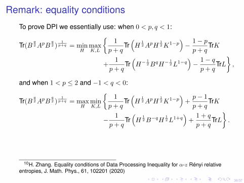
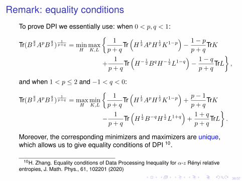
Remark: equality conditions
To prove DPI we essentially use: when 0 < p, q < 1:
Tr(Bq2ApB
q2 )
1p+q = min
HmaxK,L
{1
p+ qTr(H
12ApH
12K1−p
)− 1− pp+ q
TrK
+1
p+ qTr(H−
12BqH−
12L1−q
)− 1− qp+ q
TrL},
and when 1 < p ≤ 2 and −1 < q < 0:
Tr(Bq2ApB
q2 )
1p+q = max
HminK,L
{1
p+ qTr(H
12ApH
12K1−p
)+p− 1
p+ qTrK
− 1
p+ qTr(H
12B−qH
12L1+q
)+
1 + q
p+ qTrL}.
Moreover, the corresponding minimizers and maximizers are unique,which allows us to give equality conditions of DPI 10.
10H. Zhang. Equality conditions of Data Processing Inequality for α-z Rényi relativeentropies, J. Math. Phys., 61, 102201 (2020)
36/37
Remark: equality conditions
To prove DPI we essentially use: when 0 < p, q < 1:
Tr(Bq2ApB
q2 )
1p+q = min
HmaxK,L
{1
p+ qTr(H
12ApH
12K1−p
)− 1− pp+ q
TrK
+1
p+ qTr(H−
12BqH−
12L1−q
)− 1− qp+ q
TrL},
and when 1 < p ≤ 2 and −1 < q < 0:
Tr(Bq2ApB
q2 )
1p+q = max
HminK,L
{1
p+ qTr(H
12ApH
12K1−p
)+p− 1
p+ qTrK
− 1
p+ qTr(H
12B−qH
12L1+q
)+
1 + q
p+ qTrL}.
Moreover, the corresponding minimizers and maximizers are unique,which allows us to give equality conditions of DPI 10.
10H. Zhang. Equality conditions of Data Processing Inequality for α-z Rényi relativeentropies, J. Math. Phys., 61, 102201 (2020)
37/37
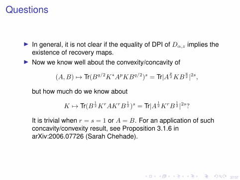
Questions
I In general, it is not clear if the equality of DPI of Dα,z implies theexistence of recovery maps.
I Now we know well about the convexity/concavity of
(A,B) 7→ Tr(Bq/2K∗ApKBq/2)s = Tr|Ap2KB
q2 |2s,
but how much do we know about
K 7→ Tr(B12KrAKrB
12 )s = Tr|A 1
2KrB12 |2s?
It is trivial when r = s = 1 or A = B. For an application of suchconcavity/convexity result, see Proposition 3.1.6 inarXiv:2006.07726 (Sarah Chehade).
37/37
Questions
I In general, it is not clear if the equality of DPI of Dα,z implies theexistence of recovery maps.
I Now we know well about the convexity/concavity of
(A,B) 7→ Tr(Bq/2K∗ApKBq/2)s = Tr|Ap2KB
q2 |2s,
but how much do we know about
K 7→ Tr(B12KrAKrB
12 )s = Tr|A 1
2KrB12 |2s?
It is trivial when r = s = 1 or A = B. For an application of suchconcavity/convexity result, see Proposition 3.1.6 inarXiv:2006.07726 (Sarah Chehade).

Thank you!
37/37