Physica D 240 (2011) 323–345

Contents lists available at ScienceDirect

Physica D

journal homepage: www.elsevier.com/locate/physd

How effective delays shape oscillatory dynamics in neuronal networksAlex Roxin a,b, Ernest Montbrió a,c,∗

a Department of Information and Communication Technologies, Universitat Pompeu Fabra, E-08018 Barcelona, Spainb Center for Theoretical Neuroscience, Columbia University, New York, NY 10032, USAc Center for Neural Science, New York University, New York, NY 10012, USA

a r t i c l e i n f o

Article history:Received 11 November 2009Received in revised form19 September 2010Accepted 20 September 2010Available online 25 September 2010Communicated by S. Coombes

Keywords:DelayNeuronal networksNeural fieldAmplitude equationsWilson–Cowan networksRate modelsOscillations

a b s t r a c t

Synaptic, dendritic and single-cell kinetics generate significant time delays that shape the dynamics oflarge networks of spiking neurons. Previous work has shown that such effective delays can be taken intoaccountwith a ratemodel through the addition of an explicit, fixeddelay (Roxin et al. (2005,2006) [29,30]).Herewe extend thiswork to account for arbitrary symmetric patterns of synaptic connectivity and genericnonlinear transfer functions. Specifically, we conduct a weakly nonlinear analysis of the dynamical statesarising via primary instabilities of the asynchronous state. In this way we determine analytically how thenature and stability of these states depend on the choice of transfer function and connectivity. We arriveat two general observations of physiological relevance that could not be explained in previouswork. Theseare: 1— fast oscillations are always supercritical for realistic transfer functions and 2— travelingwaves arepreferred over standing waves given plausible patterns of local connectivity. We finally demonstrate thatthese results show good agreement with those obtained performing numerical simulations of a networkof Hodgkin–Huxley neurons.

© 2010 Elsevier B.V. All rights reserved.

1. Introduction

When studying the collective dynamics of cortical neuronscomputationally, networks of large numbers of spiking neuronshave naturally been the benchmarkmodel. Networkmodels incor-porate the most fundamental physiological properties of neurons:sub-threshold voltage dynamics, spiking (via spike generation dy-namics or a fixed threshold), and discontinuous synaptic interac-tions. For this reason, networks of spiking neurons are consideredto be biologically realistic. However, with a few exceptions, e.g.[1–3], network models of spiking neurons are not amenable to an-alytical work and thus constitute above all a computational tool.Rather, researchers use reduced or simplified models which de-scribe some measure of the mean activity in a population of cells,oftentimes taken as the firing rate (for reviews, see [4,5]). Firing-rate models are simple, phenomenological models of neuronal ac-tivity, generally in the form of continuous, first-order ordinarydifferential equations [6,7]. Such firing-rate models can be ana-lyzed using standard techniques for differential equations, allow-ing one to understand the qualitative dependence of the dynamics

∗ Corresponding author at: Department of Information and CommunicationTechnologies, Universitat Pompeu Fabra, E-08018 Barcelona, Spain. Tel.: +34 93 5421450.

E-mail address: ernest.montbrio@upf.edu (E. Montbrió).

0167-2789/$ – see front matter© 2010 Elsevier B.V. All rights reserved.doi:10.1016/j.physd.2010.09.009

on parameters.Nonetheless, firing-ratemodels do not represent, ingeneral, proper mathematical reductions of the original networkdynamics but rather are heuristic, but see [8]. As such, there is ingeneral no clear relationship between the parameters in the ratemodel and those in the full network of spiking neurons, althoughfor at least some specific cases quasi-analytical approaches maybe of value [9]. It therefore behooves the researcher to study ratemodels in conjunctionwith network simulations in order to ensurethere is good qualitative agreement between the two.

Luckily, rate models have proven remarkably accurate in cap-turing the main types of qualitative dynamical states seen innetworks of large numbers of asynchronously spiking neurons. Forexample, it is well known that in such networks the different tem-poral dynamics of excitatory and inhibitory neurons can lead tooscillations. These oscillations can be well captured using ratemodels [6]. When the pattern of synaptic connectivity depends onthe distance between neurons, these differences in the temporaldynamics can also lead to the emergence of waves [7,10–12]. Thisis certainly a relevant case for local circuits in cortical tissue, wherethe likelihood of finding a connection between any two neuronsdecreases as a function of the distance between them, e.g. [13].

When considering the spatial dependence of the patterns ofsynaptic connectivity between neurons, one must take into ac-count the presence of time delays due to the finite velocity prop-agation of action potentials along axons. Such delays dependlinearly on the distance between any two neurons. This has been

324 A. Roxin, E. Montbrió / Physica D 240 (2011) 323–345

the topic of much theoretical study using rate models with aspace-dependent time delay e.g. [14–16,12,11,17–22]. The pres-ence of propagation delays can cause an oscillatory instability ofthe unpatterned state leading to homogeneous oscillations andwaves [15,18]. The weakly nonlinear dynamics of waves in spa-tially extended rate models, i.e. describing large-scale (on theorder of centimeters) activity, is described by the coupled mean-field Ginzburg–Landau equations [21], and thus exhibits the phe-nomenology of small amplitude waves familiar from other patternforming systems [23]. Also, it is important to note that discretefixed delays have been used to model the time delayed interactionbetween discrete neuronal regions, as well as to model neuronalfeedback, e.g. [24–28].

Localized solutions of integro-differential equations describingneuronal activity, including fronts and pulses, are also affectedbydistance-dependent axonal delays [11,12,15,17,20]. Specifically,the velocity of propagation of the localized solution is proportionalto the conduction velocity along the axon for small conductionvelocities, while for large conduction velocities it is essentiallyconstant. This reflects the fact that the propagation of activity inneuronal tissue is driven by local integration inwhich synaptic andmembrane time constants provide the bottleneck. Also, allowingfor different conduction velocities for separate excitatory andinhibitory populations can lead to bifurcations of localized bumpstates to breathers and traveling pulses [19].

Although the presence of time delays in the nervous system aremost often associated with axonal propagation, significant timedelays are also produced by the synaptic kinetics and single-celldynamics (see the next section for a detailed discussion about theorigin of such effective timedelays in networks of spikingneurons).As a relevant example for the present work, it was shown in[29,30] that the addition of an explicit, non-space-dependent delayin a rate equation was sufficient to explain the emergence of fastoscillations prevalent in networks of spiking neurons with stronginhibition and in the absence of any explicit delays.

Specifically, in [29,30] the authors studied a rate model with afixed delay on a ring geometry with two simplifying assumptions.First they assumed that the strength of connection betweenneurons could be expressed as a constant plus the cosine of thedistance between the neurons. Second, they assumed a linearrectified form for the transfer function which relates inputs tooutputs. These assumptions allowed them to construct a detailedphase diagramof dynamical states, to a large degree analytically. Inaddition to the stationary bump state (SB) which had been studiedpreviously [31,32], the presence of a delay led to two new statesarising from primary instabilities of the stationary uniform state(SU): an oscillatory uniform state (OU) and a traveling wave state(TW). Secondary bifurcations of these three states (SB, OU, TW)led to yet more complex states including standing waves (SW) andoscillatory bump states (OB). Several regions of bistability betweenprimary and secondary states were found, including OU–TW,OU–SB and OU–OB. They subsequently confirmed these resultsthrough simulations of networks of Hodgkin–Huxley neurons.Despite the good agreement between the rate equation andnetwork simulations, several important issues remain unresolved:

• The rate equation predicted that the primary instability of theSU state to waves should be to traveling waves, while in thenetwork simulations standing waves were robustly observed.

• The linear-threshold transfer function, albeit amenable to anal-ysis, nonetheless leads to degenerate behavior at a bifur-cation point. Specifically, any perturbations with a positivelinear growth rate will continue to grow until the lower thresh-old of the transfer function is reached. This means that theamplitude of new solution branches at a bifurcation is alwaysfinite, although the solution itself may not be subcritical. In a

practical sense then, this means that it is not possible to as-sess whether a particular solution, for example oscillations orbumps, will emerge continuously from the SU state as a param-eter is changed, or if it will appear at finite amplitude and there-fore be bistable with the SU state over some range.

• The previous work only considered a simplified cosine connec-tivity. More realistic patterns of synaptic connectivity such asa Gaussian dependence of connection strength as a function ofdistance might lead to different dynamical regimes. There re-mains to be explored the effect of a general connectivity kernelin the dynamics of both the rate equation and the spiking neu-ron network with fixed time delays.

In order to address these issues, and provide a more completeanalysis of the role of fixed delays in neuronal tissue, we herestudy a rate equationwith delaywithout imposing any restrictionson the form of the transfer function beyond smoothness or onthe shape of the connectivity kernel beyond being symmetric. Ourapproach is similar to that of Curtu and Ermentrout in [33], whoextended a simplified rate model with adaptation for orientationselectivity [32] to include a nonlinear transfer function and generalconnectivity kernel. Here we do the same for a rate model with afixed time delay.

Thus in what follows we will study a rate equation with fixeddelay and spatially modulated connectivity. In conjunction withthis analysiswewill conduct numerical simulations of a network oflarge numbers of spiking neurons in order to assess the qualitativeagreement between the rate model and the network for the delay-driven instabilities, which are the primary focus of this work.

This article is organized as follows: In Section 2 we providean overview of the origin of the effective delay. We do this bylooking at the dynamics of synaptically coupled conductance-based neurons. This will motivate the presence of an explicit fixeddelay in a rate-model description of the dynamics in recurrentlycoupled networks of neurons. In Section 3 we formulate the ratemodel and conduct a linear stability analysis of the SU state.In Section 4 we conduct a weakly nonlinear analysis for thefour possible primary instabilities of the SU state (asynchronousunpatterned state in a networkmodel), therebyderiving amplitudeequations for steady, Turing (bumps), Hopf (global oscillations),and Turing–Hopf (waves) bifurcations. We will focus on the delay-driven instabilities, i.e. Hopf and Turing–Hopf. Finally, in Section 5we will study the interactions of pairs of solutions: bumps andglobal oscillations, and global oscillations and waves, respectively.

2. The origin of effective time delays

This section is intended to provide an intuitive illustration of theorigin of an effective fixed delay in networks of spiking neurons.A detailed, analytical study of this phenomenon can be found in[2,34,35].

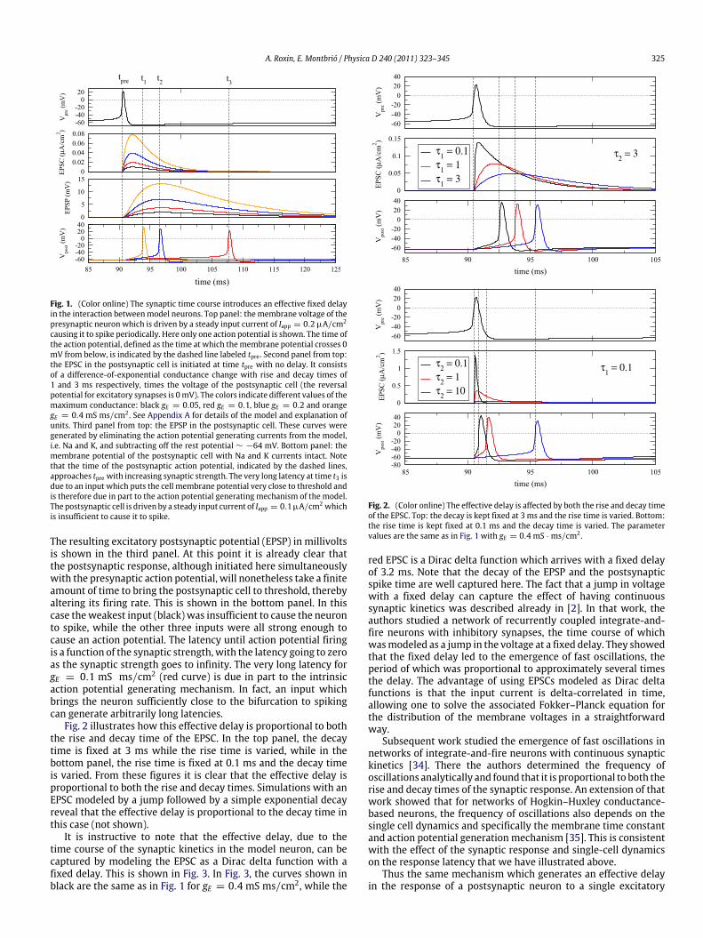
Fig. 1 illustrates the origin of the effective delay in networks ofmodel neurons. In this case we look at a single neuron pair: onepresynaptic and one postsynaptic. The single-neuron dynamics aredescribed in detail in Appendix A. The top panel of Fig. 1 shows themembrane potential of an excitatory neuron subjected to a currentinjection of Iapp = 0.2 µA/cm2 which causes it to fire actionpotentials. Numerically, an action potential is detected wheneverthe membrane voltage exceeds 0 mV from below. When thisoccurs, an excitatory postsynaptic current (EPSC) is generated inthe post-synaptic neuron, as seen in the second panel. This currentis generated by the activation of an excitatory conductance whichhas the functional form of a difference of exponentials with risetime τ1 = 1 ms and decay time τ2 = 3 ms. The different coloredcurves correspond to different conductance strengths: black gE =

0.05, red gE = 0.1, blue gE = 0.2 and orange gE = 0.4mSms/cm2.

A. Roxin, E. Montbrió / Physica D 240 (2011) 323–345 325

Fig. 1. (Color online) The synaptic time course introduces an effective fixed delayin the interaction betweenmodel neurons. Top panel: themembrane voltage of thepresynaptic neuron which is driven by a steady input current of Iapp = 0.2 µA/cm2

causing it to spike periodically. Here only one action potential is shown. The time ofthe action potential, defined as the time at which themembrane potential crosses 0mV from below, is indicated by the dashed line labeled tpre . Second panel from top:the EPSC in the postsynaptic cell is initiated at time tpre with no delay. It consistsof a difference-of-exponential conductance change with rise and decay times of1 and 3 ms respectively, times the voltage of the postsynaptic cell (the reversalpotential for excitatory synapses is 0mV). The colors indicate different values of themaximum conductance: black gE = 0.05, red gE = 0.1, blue gE = 0.2 and orangegE = 0.4 mS ms/cm2 . See Appendix A for details of the model and explanation ofunits. Third panel from top: the EPSP in the postsynaptic cell. These curves weregenerated by eliminating the action potential generating currents from the model,i.e. Na and K, and subtracting off the rest potential ∼ −64 mV. Bottom panel: themembrane potential of the postsynaptic cell with Na and K currents intact. Notethat the time of the postsynaptic action potential, indicated by the dashed lines,approaches tpre with increasing synaptic strength. The very long latency at time t3 isdue to an input which puts the cell membrane potential very close to threshold andis therefore due in part to the action potential generating mechanism of the model.The postsynaptic cell is driven by a steady input current of Iapp = 0.1µA/cm2 whichis insufficient to cause it to spike.

The resulting excitatory postsynaptic potential (EPSP) in millivoltsis shown in the third panel. At this point it is already clear thatthe postsynaptic response, although initiated here simultaneouslywith the presynaptic action potential, will nonetheless take a finiteamount of time to bring the postsynaptic cell to threshold, therebyaltering its firing rate. This is shown in the bottom panel. In thiscase theweakest input (black) was insufficient to cause the neuronto spike, while the other three inputs were all strong enough tocause an action potential. The latency until action potential firingis a function of the synaptic strength, with the latency going to zeroas the synaptic strength goes to infinity. The very long latency forgE = 0.1 mS ms/cm2 (red curve) is due in part to the intrinsicaction potential generating mechanism. In fact, an input whichbrings the neuron sufficiently close to the bifurcation to spikingcan generate arbitrarily long latencies.

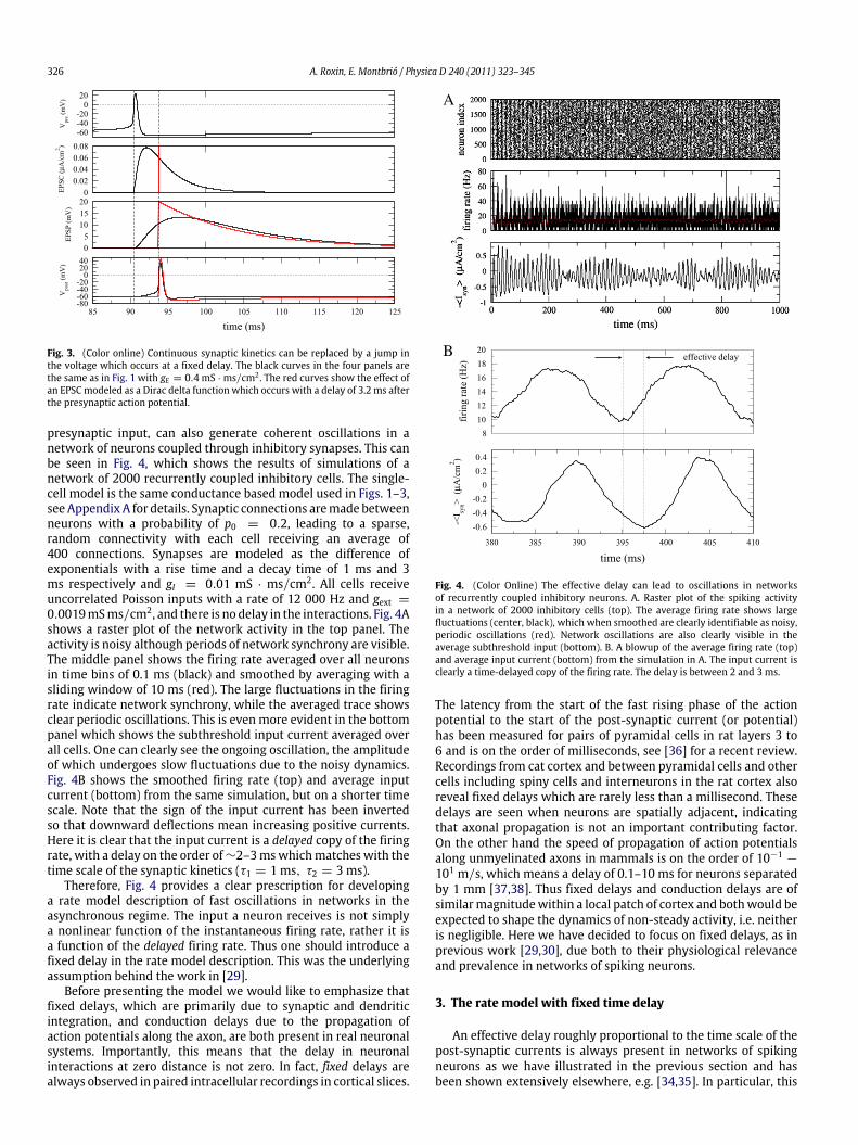
Fig. 2 illustrates how this effective delay is proportional to boththe rise and decay time of the EPSC. In the top panel, the decaytime is fixed at 3 ms while the rise time is varied, while in thebottom panel, the rise time is fixed at 0.1 ms and the decay timeis varied. From these figures it is clear that the effective delay isproportional to both the rise and decay times. Simulations with anEPSC modeled by a jump followed by a simple exponential decayreveal that the effective delay is proportional to the decay time inthis case (not shown).

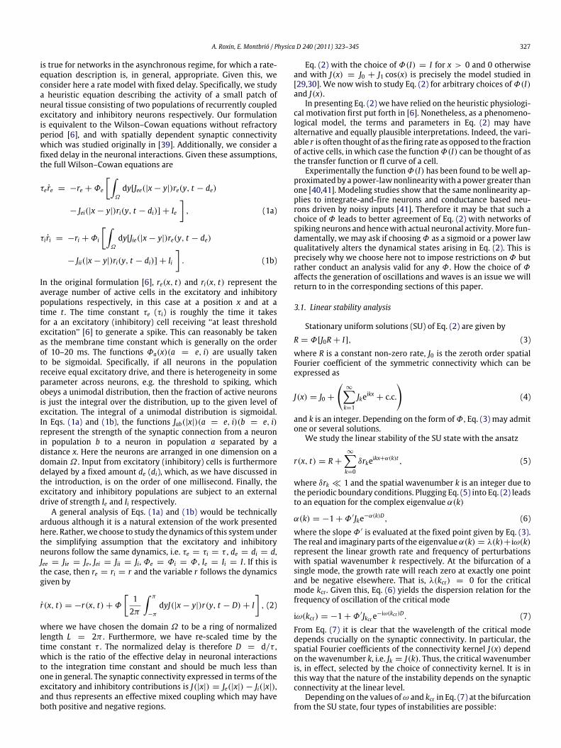
It is instructive to note that the effective delay, due to thetime course of the synaptic kinetics in the model neuron, can becaptured by modeling the EPSC as a Dirac delta function with afixed delay. This is shown in Fig. 3. In Fig. 3, the curves shown inblack are the same as in Fig. 1 for gE = 0.4 mS ms/cm2, while the

Fig. 2. (Color online) The effective delay is affected by both the rise and decay timeof the EPSC. Top: the decay is kept fixed at 3 ms and the rise time is varied. Bottom:the rise time is kept fixed at 0.1 ms and the decay time is varied. The parametervalues are the same as in Fig. 1 with gE = 0.4 mS · ms/cm2 .

red EPSC is a Dirac delta function which arrives with a fixed delayof 3.2 ms. Note that the decay of the EPSP and the postsynapticspike time are well captured here. The fact that a jump in voltagewith a fixed delay can capture the effect of having continuoussynaptic kinetics was described already in [2]. In that work, theauthors studied a network of recurrently coupled integrate-and-fire neurons with inhibitory synapses, the time course of whichwasmodeled as a jump in the voltage at a fixed delay. They showedthat the fixed delay led to the emergence of fast oscillations, theperiod of which was proportional to approximately several timesthe delay. The advantage of using EPSCs modeled as Dirac deltafunctions is that the input current is delta-correlated in time,allowing one to solve the associated Fokker–Planck equation forthe distribution of the membrane voltages in a straightforwardway.

Subsequent work studied the emergence of fast oscillations innetworks of integrate-and-fire neurons with continuous synaptickinetics [34]. There the authors determined the frequency ofoscillations analytically and found that it is proportional to both therise and decay times of the synaptic response. An extension of thatwork showed that for networks of Hogkin–Huxley conductance-based neurons, the frequency of oscillations also depends on thesingle cell dynamics and specifically the membrane time constantand action potential generation mechanism [35]. This is consistentwith the effect of the synaptic response and single-cell dynamicson the response latency that we have illustrated above.

Thus the same mechanism which generates an effective delayin the response of a postsynaptic neuron to a single excitatory

326 A. Roxin, E. Montbrió / Physica D 240 (2011) 323–345

Fig. 3. (Color online) Continuous synaptic kinetics can be replaced by a jump inthe voltage which occurs at a fixed delay. The black curves in the four panels arethe same as in Fig. 1 with gE = 0.4 mS · ms/cm2 . The red curves show the effect ofan EPSCmodeled as a Dirac delta function which occurs with a delay of 3.2 ms afterthe presynaptic action potential.

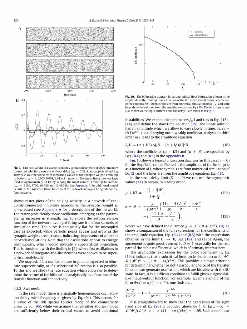
presynaptic input, can also generate coherent oscillations in anetwork of neurons coupled through inhibitory synapses. This canbe seen in Fig. 4, which shows the results of simulations of anetwork of 2000 recurrently coupled inhibitory cells. The single-cell model is the same conductance based model used in Figs. 1–3,see Appendix A for details. Synaptic connections aremade betweenneurons with a probability of p0 = 0.2, leading to a sparse,random connectivity with each cell receiving an average of400 connections. Synapses are modeled as the difference ofexponentials with a rise time and a decay time of 1 ms and 3ms respectively and gI = 0.01 mS · ms/cm2. All cells receiveuncorrelated Poisson inputs with a rate of 12 000 Hz and gext =

0.0019mSms/cm2, and there is no delay in the interactions. Fig. 4Ashows a raster plot of the network activity in the top panel. Theactivity is noisy although periods of network synchrony are visible.The middle panel shows the firing rate averaged over all neuronsin time bins of 0.1 ms (black) and smoothed by averaging with asliding window of 10 ms (red). The large fluctuations in the firingrate indicate network synchrony, while the averaged trace showsclear periodic oscillations. This is even more evident in the bottompanel which shows the subthreshold input current averaged overall cells. One can clearly see the ongoing oscillation, the amplitudeof which undergoes slow fluctuations due to the noisy dynamics.Fig. 4B shows the smoothed firing rate (top) and average inputcurrent (bottom) from the same simulation, but on a shorter timescale. Note that the sign of the input current has been invertedso that downward deflections mean increasing positive currents.Here it is clear that the input current is a delayed copy of the firingrate, with a delay on the order of∼2–3mswhichmatcheswith thetime scale of the synaptic kinetics (τ1 = 1 ms, τ2 = 3 ms).

Therefore, Fig. 4 provides a clear prescription for developinga rate model description of fast oscillations in networks in theasynchronous regime. The input a neuron receives is not simplya nonlinear function of the instantaneous firing rate, rather it isa function of the delayed firing rate. Thus one should introduce afixed delay in the rate model description. This was the underlyingassumption behind the work in [29].

Before presenting the model we would like to emphasize thatfixed delays, which are primarily due to synaptic and dendriticintegration, and conduction delays due to the propagation ofaction potentials along the axon, are both present in real neuronalsystems. Importantly, this means that the delay in neuronalinteractions at zero distance is not zero. In fact, fixed delays arealways observed in paired intracellular recordings in cortical slices.

A

B

Fig. 4. (Color Online) The effective delay can lead to oscillations in networksof recurrently coupled inhibitory neurons. A. Raster plot of the spiking activityin a network of 2000 inhibitory cells (top). The average firing rate shows largefluctuations (center, black), which when smoothed are clearly identifiable as noisy,periodic oscillations (red). Network oscillations are also clearly visible in theaverage subthreshold input (bottom). B. A blowup of the average firing rate (top)and average input current (bottom) from the simulation in A. The input current isclearly a time-delayed copy of the firing rate. The delay is between 2 and 3 ms.

The latency from the start of the fast rising phase of the actionpotential to the start of the post-synaptic current (or potential)has been measured for pairs of pyramidal cells in rat layers 3 to6 and is on the order of milliseconds, see [36] for a recent review.Recordings from cat cortex and between pyramidal cells and othercells including spiny cells and interneurons in the rat cortex alsoreveal fixed delays which are rarely less than a millisecond. Thesedelays are seen when neurons are spatially adjacent, indicatingthat axonal propagation is not an important contributing factor.On the other hand the speed of propagation of action potentialsalong unmyelinated axons in mammals is on the order of 10−1

−

101 m/s, which means a delay of 0.1–10 ms for neurons separatedby 1 mm [37,38]. Thus fixed delays and conduction delays are ofsimilarmagnitudewithin a local patch of cortex and bothwould beexpected to shape the dynamics of non-steady activity, i.e. neitheris negligible. Here we have decided to focus on fixed delays, as inprevious work [29,30], due both to their physiological relevanceand prevalence in networks of spiking neurons.

3. The rate model with fixed time delay

An effective delay roughly proportional to the time scale of thepost-synaptic currents is always present in networks of spikingneurons as we have illustrated in the previous section and hasbeen shown extensively elsewhere, e.g. [34,35]. In particular, this

A. Roxin, E. Montbrió / Physica D 240 (2011) 323–345 327

is true for networks in the asynchronous regime, for which a rate-equation description is, in general, appropriate. Given this, weconsider here a rate model with fixed delay. Specifically, we studya heuristic equation describing the activity of a small patch ofneural tissue consisting of two populations of recurrently coupledexcitatory and inhibitory neurons respectively. Our formulationis equivalent to the Wilson–Cowan equations without refractoryperiod [6], and with spatially dependent synaptic connectivitywhich was studied originally in [39]. Additionally, we consider afixed delay in the neuronal interactions. Given these assumptions,the full Wilson–Cowan equations are

τe re = −re + Φe

[∫Ω

dy[Jee(|x − y|)re(y, t − de)

− Jei(|x − y|)ri(y, t − di)] + Ie

], (1a)

τi ri = −ri + Φi

[∫Ω

dy[Jie(|x − y|)re(y, t − de)

− Jii(|x − y|)ri(y, t − di)] + Ii

]. (1b)

In the original formulation [6], re(x, t) and ri(x, t) represent theaverage number of active cells in the excitatory and inhibitorypopulations respectively, in this case at a position x and at atime t . The time constant τe (τi) is roughly the time it takesfor a an excitatory (inhibitory) cell receiving ‘‘at least thresholdexcitation’’ [6] to generate a spike. This can reasonably be takenas the membrane time constant which is generally on the orderof 10–20 ms. The functions Φa(x)(a = e, i) are usually takento be sigmoidal. Specifically, if all neurons in the populationreceive equal excitatory drive, and there is heterogeneity in someparameter across neurons, e.g. the threshold to spiking, whichobeys a unimodal distribution, then the fraction of active neuronsis just the integral over the distribution, up to the given level ofexcitation. The integral of a unimodal distribution is sigmoidal.In Eqs. (1a) and (1b), the functions Jab(|x|)(a = e, i)(b = e, i)represent the strength of the synaptic connection from a neuronin population b to a neuron in population a separated by adistance x. Here the neurons are arranged in one dimension on adomain Ω . Input from excitatory (inhibitory) cells is furthermoredelayed by a fixed amount de (di), which, as we have discussed inthe introduction, is on the order of one millisecond. Finally, theexcitatory and inhibitory populations are subject to an externaldrive of strength Ie and Ii respectively.

A general analysis of Eqs. (1a) and (1b) would be technicallyarduous although it is a natural extension of the work presentedhere. Rather, we choose to study the dynamics of this systemunderthe simplifying assumption that the excitatory and inhibitoryneurons follow the same dynamics, i.e. τe = τi = τ , de = di = d,Jee = Jie = Je, Jei = Jii = Ji, Φe = Φi = Φ , Ie = Ii = I . If this isthe case, then re = ri = r and the variable r follows the dynamicsgiven by

r(x, t) = −r(x, t)+ Φ

[12π

∫ π

−π

dyJ(|x − y|)r(y, t − D)+ I], (2)

where we have chosen the domain Ω to be a ring of normalizedlength L = 2π . Furthermore, we have re-scaled time by thetime constant τ . The normalized delay is therefore D = d/τ ,which is the ratio of the effective delay in neuronal interactionsto the integration time constant and should be much less thanone in general. The synaptic connectivity expressed in terms of theexcitatory and inhibitory contributions is J(|x|) = Je(|x|) − Ji(|x|),and thus represents an effective mixed coupling which may haveboth positive and negative regions.

Eq. (2) with the choice of Φ(I) = I for x > 0 and 0 otherwiseand with J(x) = J0 + J1 cos(x) is precisely the model studied in[29,30]. We now wish to study Eq. (2) for arbitrary choices ofΦ(I)and J(x).

In presenting Eq. (2) we have relied on the heuristic physiologi-cal motivation first put forth in [6]. Nonetheless, as a phenomeno-logical model, the terms and parameters in Eq. (2) may havealternative and equally plausible interpretations. Indeed, the vari-able r is often thought of as the firing rate as opposed to the fractionof active cells, in which case the functionΦ(I) can be thought of asthe transfer function or fI curve of a cell.

Experimentally the functionΦ(I) has been found to be well ap-proximated by a power-lawnonlinearitywith a power greater thanone [40,41]. Modeling studies show that the same nonlinearity ap-plies to integrate-and-fire neurons and conductance based neu-rons driven by noisy inputs [41]. Therefore it may be that such achoice of Φ leads to better agreement of Eq. (2) with networks ofspiking neurons and hencewith actual neuronal activity.More fun-damentally, we may ask if choosingΦ as a sigmoid or a power lawqualitatively alters the dynamical states arising in Eq. (2). This isprecisely why we choose here not to impose restrictions onΦ butrather conduct an analysis valid for any Φ . How the choice of Φaffects the generation of oscillations and waves is an issue we willreturn to in the corresponding sections of this paper.

3.1. Linear stability analysis

Stationary uniform solutions (SU) of Eq. (2) are given by

R = Φ[J0R + I], (3)

where R is a constant non-zero rate, J0 is the zeroth order spatialFourier coefficient of the symmetric connectivity which can beexpressed as

J(x) = J0 +

∞−k=1

Jkeikx + c.c.

(4)

and k is an integer. Depending on the form ofΦ , Eq. (3) may admitone or several solutions.

We study the linear stability of the SU state with the ansatz

r(x, t) = R +

∞−k=0

δrkeikx+α(k)t , (5)

where δrk ≪ 1 and the spatial wavenumber k is an integer due tothe periodic boundary conditions. Plugging Eq. (5) into Eq. (2) leadsto an equation for the complex eigenvalue α(k)

α(k) = −1 + Φ ′Jke−α(k)D, (6)

where the slopeΦ ′ is evaluated at the fixed point given by Eq. (3).The real and imaginary parts of the eigenvalueα(k) = λ(k)+iω(k)represent the linear growth rate and frequency of perturbationswith spatial wavenumber k respectively. At the bifurcation of asingle mode, the growth rate will reach zero at exactly one pointand be negative elsewhere. That is, λ(kcr) = 0 for the criticalmode kcr. Given this, Eq. (6) yields the dispersion relation for thefrequency of oscillation of the critical mode

iω(kcr) = −1 + Φ ′Jkcre−iω(kcr)D. (7)

From Eq. (7) it is clear that the wavelength of the critical modedepends crucially on the synaptic connectivity. In particular, thespatial Fourier coefficients of the connectivity kernel J(x) dependon the wavenumber k, i.e. Jk = J(k). Thus, the critical wavenumberis, in effect, selected by the choice of connectivity kernel. It is inthis way that the nature of the instability depends on the synapticconnectivity at the linear level.

Depending on the values ofω and kcr in Eq. (7) at the bifurcationfrom the SU state, four types of instabilities are possible:

328 A. Roxin, E. Montbrió / Physica D 240 (2011) 323–345

• Steady (ω = 0, kcr = 0): the instability leads to a globalincrease in activity.

• Turing (ω = 0, kcr = 0): the instability leads to a stationarybump state (SU).

• Hopf (ω = 0, kcr = 0): the instability leads to an oscillatoryuniform state (OU).

• Turing–Hopf (ω = 0, kcr = 0): the instability leads to waves(SW, TW).

For the non-oscillatory instabilities (i.e.ω = 0), Eq. (7) gives thecritical value

Jk = 1/Φ ′ (8)

while for the oscillatory ones Eq. (7) is equivalent to the system oftwo transcendental equations

ω = − tan ωD, (9a)

ω = −Φ ′ Jk sin ωD. (9b)

Note that we have defined the critical values as Jkcr ≡ Jk andωcr ≡ ω.

3.1.1. The small delay limit (D → 0)It is possible to gain some intuition regarding the effect of

fixed delays on the dynamics, by deriving asymptotic results inthe limit of small delay. This limit is a relevant one physiologically,since fixed delays are on the order of a few milliseconds and theintegration time constant is about an order of magnitude larger.Therefore throughout thisworkwewill present asymptotic results,and compare them to the full analytical formulas as well as tonumerical simulations.

In the limit D → 0, the asymptotic solutions of Eq. (9a) canbe easily obtained graphically. Fig. 5 shows two curves (blackand grey) representing the right and left hand sides of Eq. (9a)respectively, where we defined φ ≡ ωD. The intersections ofthese curves correspond to the roots of Eq. (9a). The plot showsthree solutions, the trivial one φ = 0 (corresponding to the non-oscillatory instabilities), and two solutions that clearly approachφ = ±π/2 in the small delay limit, since the slope of the straightline goes to infinity as D → 0. Substituting these solutions into Eq.(9b), we find that the first potentially unstable solution of the kthspatial Fourier mode is φ = π/2, that occurs at the critical valueof the coupling

Jk = −π

2DΦ ′, (10)

with a frequency

ω =π

2D. (11)

Fig. 6 shows the critical frequency and coupling as a function ofthe delay, up to a delay D = 1. The solution obtained from thedispersion relation equations (9a) and (9b) are given by solid lines,while the expressions obtained in the small delay limit are givenby dotted lines. Thus the expressions in the small delay limit agreequite well with the full expressions even for D = 1.

3.2. An illustrative phase diagram

Throughout the analysis which follows we will illustrate ourresults with a phase diagram of dynamical states. Specifically,we will follow the analysis in [29,30] in constructing a phasediagram of dynamical states as a function of J0 and J1, the first twoFourier coefficients of the synaptic connectivity. We will set thehigher order coefficients to zero for this particular phase diagram,although we will discuss the effect of additional modes in the text.Furthermore, unless otherwise noted, for simulations we choose

Fig. 5. The critical frequency at the instability to oscillations is given by theintersection of the grey (D = 0.1) and black curves, the left and right hand sidesof Eq. (9a) respectively. As D → 0, solutions clearly approach φ = (2n + 1)π/2 (ninteger). Eq. (9b) shows that the first potentially unstable mode corresponds to thesolutions φ = ±π/2 (see text).

ωcr

0.1 1

D

-Jcr

1

10

100

1

10

100

1000

Fig. 6. Top: the critical frequency of oscillatory instabilities as a function of thedelay D from the dispersion equation Eq. (9a) (solid line) and in the small delaylimit (dotted line). Bottom: the critical coupling as a function of the delay D fromEq. (9b) (solid) and in the small delay limit (dotted).

a sigmoidal transfer function Φ(I) =α

1+e−βIwith α = 1.5 and

β = 3. As we vary the connectivity in the phase diagram, we alsovary the constant input I in order to maintain the same level ofmean activity, i.e. we keep R = 0.1 fixed. For the values of theparameters we have chosen here this results in I ∼ −0.1J0 − 0.88.We also take D = 0.1 unless noted otherwise

The primary instability lines for the SU state can be seenin the phase diagram, Fig. 7. The region in (J0, J1) space wherethe SU state is stable is shown in gray, while the primaryinstabilities, listed above, are shown as red lines. In Section 4 wewill provide a detailed analysis of the bumps, global oscillationsand waves (SB, OU and SW/TW) which arise due to the Turing,Hopf and Turing–Hopf instabilities respectively. The derivation ofthe amplitude equations is given in Appendix B, as well as a briefdiscussion of the steady, transcritical bifurcation which occurs forstrong excitatory coupling and is not of primary interest for thisstudy. Finally, in Section 5 we will analyze the codimension 2bifurcations: Hopf and Turing–Hopf (OU and waves), and Turingand Hopf (SU and OU). This analysis will allow us to understandthe dynamical states which appear near the upper and lower lefthand corners of the grey shaded region in Fig. 7, i.e. the SW/OU andOB states.

4. Bifurcations of codimension 1

As we are interested in creating a phase diagram as a functionof the connectivity, we will take changes in the connectivity as the

A. Roxin, E. Montbrió / Physica D 240 (2011) 323–345 329

J0

J 1

SU

SB

HA

OU

TW

OB SB/HA

TW/HA

SW

SU/HA

SU/SWSW

TW/SWSW/OU

Turing-Hopf

Turing

Tra

nscr

itica

l

Hop

f0

-100

-50

-100 -50 0

Fig. 7. (Color online) Phase diagram of the rate model Eq. (2). In each region, thetype of solution seen in numerical simulations is indicated by a letter code: SU —stationary uniform (grey region), HA — high activity, SB — stationary bump, OB —oscillatory bump, SW— standing waves, TW— traveling waves. Solid lines indicateanalytical expressions. In particular, the four possible instabilities of the SU state aredepicted in red (thick lines correspond to subcritical bifurcations) and are given bythe linear stability criteria Eqs. (8) and (9b). The four lines emanating from the upperand lower left corners of the SU region were determined from a weakly nonlinearanalysis at the two corners (codimension 2 points) [see Section 4]. The regionmarked OB corresponds to a mixed mode solution of SB–OU, while in the lowerleft-hand region the OU and SW solutions are bistable. Parameters:Φ(x) =

α

1+e−βx

where α = 1.5 and β = 3. We consider the coupling function J(x) = J0 + 2J1 cos x.The time delay is D = 0.1 and the input current I is varied so as to keep the uniformstationary solution fixed at R = 0.1.

bifurcation parameter. The small parameter ϵ is therefore definedby the expansion

Jk = Jk + ϵ2∆Jk. (12)

The perturbative method we apply, which makes use of thissmall parameter, is called the multiple-scales method and is astandard approach for determining the weakly nonlinear behaviorof pattern-forming instabilities [23]. We choose the particularscaling of ϵ2 in the foreknowledge that if the amplitudes of thepatterns of interest are scaled as ϵ, a solvability conditionwill ariseat order ϵ3. This solvability condition yields a dynamical equationgoverning the temporal evolution of the pattern (see Appendix Afor details). Without loss of generality we will assume that aninstability of a nonzero spatial wavenumber is for k = 1. We willfurthermore co-expand the constant input I so as to maintain afixed value for the spatially homogeneous steady state solution R

I = I + ϵ2∆I, (13)

r = R + ϵr1 + ϵ2r2 + · · · , (14)

where the small parameter ϵ is defined by Eq. (12). Additionallywedefine the slow time

T = ϵ2t. (15)

4.1. Turing bifurcation

The emergence and nature of stationary bumps in rateequations have been extensively studied elsewhere, e.g. [39]. Webriefly describe this state here for completeness. The kth spatialFourier mode of the connectivity is given by the critical value Eq.(8), while we assume that all other Fourier modes are sufficientlybelow their critical values to avoid additional instabilities.Withoutloss of generality we assume k = 1 here.

We expand the parameters J1, I and r as in Eqs. (12)–(14), anddefine the slow time Eq. (15). The solution of Eq. (2) linearizedabout the SU state R is a spatially periodic amplitude which we

J2

J 0

Subcritical

Supercritical

+ + +-- - - -

0

-60

-40

-20

-60 -40 -20 0

Fig. 8. (Color online) The phase diagram for stationary bumps as a function ofthe zeroth and second spatial Fourier modes of the connectivity kernel. The regionof bistability between the unpatterned and the bump state is shaded. Here thecritical spatial Fourier coefficient J1 = 3.54. Red lines indicate the boundaries ofthe SU state (obtained via Eqs. (8) and (9b)). The functionsΦ and J(x) as well as theinput current I and the delay D are taken as in Fig. 7. Insets: example connectivitypatterns corresponding to the values of J0 and J2 marked by the square and trianglerespectively. Note that standardMexican Hat connectivity tends to favor bistability.

allow to vary slowly in time, i.e. r1 = A(T )eix + c.c. Carrying out aweakly nonlinear analysis to third order in ϵ leads to the amplitudeequation

∂TA = η∆J1A + Γ |A|2A, (16)

with the coefficients

η =Φ ′

1 + D, (17a)

Γ =J31

1 + D

J0(Φ ′′)2

1 − J0Φ ′+

J2(Φ ′′)2

2(1 − J2Φ ′)+Φ ′′′

2

. (17b)

The nature of the bifurcation (sub- or supercritical) clearlydepends strongly on the sign and magnitude of mean connectivityJ0 and the second spatial Fourier mode J2. Fig. 8 shows a phasediagram of the bump state at the critical value of J1 = 3.54. Thered lines indicate oscillatory and steady instability boundaries forthe modes J0 and J2. Clearly J0 < 0 and J2 < 0 over most of theregion of allowable values, and the bump is therefore supercritical.There is only a narrow region of predominantly positive values(shaded region in Fig. 8) for which the cubic coefficient is positive.This indicates that the bifurcating solution branch is unstable.However, neuronal activity is bounded, which is captured in Eq.(2) by a saturating transfer functionΦ . Thus the instability will notgrow without bounds but rather will saturate, producing a finiteamplitude bump solution. This stable, large amplitude branch andthe unstable branch annihilate in a saddle–node bifurcation forvalues of J1 below the critical value for the Turing instability.Such finite-amplitude bumps are therefore bistable with the SUstate. In Fig. 8, the two insets show the connectivity kernel J(x)for parameter values given by the placement of the open triangle(subcritical bump) and the open square (supercritical bump).

In the phase diagram (Fig. 7), the Turing instability line (upperhorizontal red line) is shown thin for supercritical, and thick forsubcritical bumps (here J2 = 0).

4.2. Hopf bifurcation

4.2.1. Network simulationsAs shown elsewhere previously [2,3,29], a network of recur-

rently coupled inhibitory neurons can generate fast oscillationsdue to the effective delay in the synaptic interactions. Fig. 9A

330 A. Roxin, E. Montbrió / Physica D 240 (2011) 323–345

2000 2050 2100

time (ms)2150 2200

A

B

Fig. 9. Fast oscillations in a sparse, randomly connected network of 2000 randomlyconnected inhibitory neurons without delay (pI0 = 0.2). A: raster plots of spikingactivity in four networks with increasing values of the synaptic weight. From topto bottom: gI = 0, 0.005, 0.008, 0.01 mS · ms/cm2 . The mean firing rate was keptfixed at approximately 14 Hz by varying the input current. From top to bottom:νext = 2150, 7700, 10 000 and 12 000 Hz. See Appendix A for additional modeldetails. B: the autocorrelation function of the network-averaged firing rate for thefour networks.

shows raster plots of the spiking activity in a network of ran-domly connected inhibitory neurons as the synaptic weight gIis increased (see Appendix A for a description of the network).The raster plots clearly show oscillations emerging as the param-eter gI increases in strength. Fig. 9B shows the autocorrelationfunction of the network-averaged firing rate from four seconds ofsimulation time. The curve is completely flat for the uncoupledcase as expected, while periodic peaks appear and grow as thesynapticweights are increased, indicating the presence of coherentnetwork oscillations. Note that the oscillations appear to emergecontinuously, which would indicate a supercritical bifurcation.This is consistent with the finding in [2], where fast oscillations ina network of integrate-and-fire neurons were shown to be super-critical analytically.

We may ask if fast oscillations are in general expected to bifur-cate supercritically, or if a subcritical bifurcation is also possible.To this end we study the rate equation which allows us to deter-mine the nature of the bifurcation analytically as a function of thetransfer function and connectivity.

4.2.2. Rate modelIn the rate model there is a spatially homogeneous oscillatory

instability with frequency ω given by Eq. (9a). This occurs fora value of the 0th spatial Fourier mode of the connectivitygiven by Eq. (9b), while we assume that all other Fourier modesare sufficiently below their critical values to avoid additional

J0

0

0.01

LC

am

plitu

de

numericsamplitude eqs.

-64 -62 -60 -58 -56

Fig. 10. The bifurcation diagram for a supercritical Hopf bifurcation. Shown is theamplitude of the limit cycle as a function of the 0th order spatial Fourier coefficientof the coupling J(x). Open circles are from numerical simulation of Eq. (2) and solidlines show the solution from the amplitude equation, Eq. (16). The functionsΦ andJ(x) as well as the input current I and the delay D are taken as in Fig. 7.

instabilities. We expand the parameters J0, I and r as in Eqs. (12)–(14), and define the slow time equation (15). The linear solutionhas an amplitude which we allow to vary slowly in time, i.e. r1 =

H(T )eiωt + c.c. Carrying out a weakly nonlinear analysis to thirdorder in ϵ leads to the amplitude equation

∂TH = (µ+ iΩ)∆J0H + (α + iβ)|H|2H, (18)

where the coefficients (µ + iΩ) and (α + iβ) are specified byEqs. (B.4) and (B.5) in the Appendix B.

Fig. 10 shows a typical bifurcation diagram (in this case J1 = 0)for the Hopf bifurcation. Plotted is the amplitude of the limit cycleas a function of J0 where symbols are from numerical simulation ofEq. (2) and the lines are from the amplitude equation, Eq. (18).

In the small delay limit (D → 0) we can use the asymptoticvalues (11) to obtain, to leading order,

µ+ iΩ = −

π2 + i

Φ ′

1 +π2

4

, (19a)

α + iβ = −χ

(DΦ ′)3

11π − 4

20(Φ ′′)2

Φ ′−πΦ ′′′

4

− i[11 + π

10−Φ ′′′

2

], (19b)

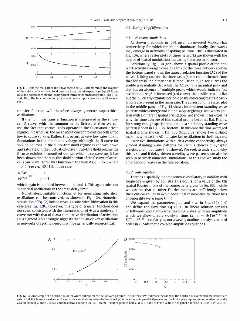
where we have defined the quantity χ ≡ π3/(8 + 2π2). Fig. 11shows a comparison of the full expressions for the coefficients ofthe amplitude equation, Eqs. (B.4) and (B.5) with the expressionsobtained in the limit D → 0, Eqs. (19a) and (19b). Again, theagreement is quite good, even up to D = 1, especially for the realpart of the cubic coefficient α, which is of primary interest here.

The asymptotic expression for the cubic coefficient α, Eq.(19b), indicates that a subcritical limit cycle should occur for Φ ′′′

Φ ′/(Φ ′′)2 > (11π − 4)/(5π). This provides a simple criterionfor determining whether or not a particular choice of the transferfunction can generate oscillations which are bistable with the SUstate. In fact, it is a difficult condition to fulfill given a sigmoidal-like input–output function. For example, given a sigmoid of theformΦ(x) = α/(1 + e−βx), one finds that

Φ ′′′Φ ′

(Φ ′′)2= 1 − 2

e−3βx

(e−4βx − 2e−3βx + e−2βx). (20)

It is straightforward to show that the expression of the righthand side of Eq. (20) is bounded above by 1. In fact, −∞ ≤

Φ ′′′Φ ′/(Φ ′′)2 < 1 < (11 − 4π)/(5π) ∼ 1.95. Such a nonlinear

A. Roxin, E. Montbrió / Physica D 240 (2011) 323–345 331

η

D

1

-α

-0.16

-0.12

-0.08

1000

1e+06

0 0.2 0.4 0.6 0.8 1

Fig. 11. Top: the real part of the linear coefficient µ. Bottom: minus the real partof the cubic coefficient −α. Solid lines are from the full expressions Eqs. (B.4) and(B.5) and dotted lines are the leading order terms in the small delay limit, Eqs. (19a)and (19b). The functions Φ and J(x) as well as the input current I are taken as inFig. 7.

transfer function will therefore always generate supercriticaloscillations.

If the nonlinear transfer function is interpreted as the single-cell fI curve, which is common in the literature, then we canuse the fact that cortical cells operate in the fluctuation-drivenregime. In particular, the mean input current to cortical cells is toolow to cause spiking. Rather, this occurs at very low rates due tofluctuations in the membrane voltage. Although the fI curve forspiking neurons in the supra-threshold regime is concave downand saturates, in the fluctuation-driven, sub-threshold regime thefI curve exhibits a smoothed-out tail which is concave up. It hasbeen shown that the sub-threshold portion of the fI curve of actualcells can bewell fitted by a function of the formΦ(x) = Axγ , whereγ > 1 (see e.g. [40,41]). In this case

Φ ′′′Φ ′

(Φ ′′)2= 1 −

1γ − 1

,

which again is bounded between −∞ and 1. This again rules outsubcritical oscillations in the small delay limit.

Nonetheless, suitable functions Φ for generating subcriticaloscillations can be contrived, as shown in Fig. 12A. Numericalsimulation of Eq. (2) indeed reveals a subcritical bifurcation in thiscase (see Fig. 12B). However, this type of transfer function doesnot seem consistent with the interpretation ofΦ as a single-cell fIcurve, nor with that ofΦ as a cumulative distribution of activation,i.e. a sigmoid. This strongly suggests that delay-driven oscillationsin networks of spiking neurons will be generically supercritical.

4.3. Turing–Hopf bifurcation

4.3.1. Network simulationsAs shown previously in [29], given an inverted Mexican-hat

connectivity for which inhibition dominates locally, fast wavesmay emerge in networks of spiking neurons. This is illustrated inFig. 13A, where raster plots of three networks are shown with thedegree of spatial modulation increasing from top to bottom.

Additionally, Fig. 13B (top) shows a spatial profile of the net-work activity averaged over 2500ms for the three networks, whilethe bottom panel shows the autocorrelation function (AC) of thenetwork firing rate for the three cases (same color scheme). Notethat for small inhibitory spatial modulation pI1 (black curve) theprofile is essentially flat while the AC exhibits an initial peak anddip, but an absence of multiple peaks which would indicate fastoscillations. As pI1 is increased (red curve), the profile remains flatbut the AC clearly exhibits periodic peaks indicating that fast oscil-lations are present in the firing rate. The corresponding raster plotin the middle panel of Fig. 13 shows intermittent standing wavepatternswhich emerge and later disappear giving rise to a newpat-tern with a different spatial orientation (not shown). This explainswhy the time average of this spatial profile becomes flat. Finally,for strong enough spatial modulation, a stationary standing wavepattern is seen in Fig. 13A (bottom). In this case the time-averagedspatial profile shown in Fig. 13B (top, blue) shows two distinctmaxima,whereas theAC indicates fast oscillations in the firing rate.

Extensive simulations with such a cosine connectivity alwaysyielded standing wave patterns for various choices of synapticweights and input rates (not shown). We seek to understand whythis is so, and if delay-driven traveling wave patterns can also beseen in network numerical simulations. To this end we study theemergence of waves in the rate equation.

4.3.2. Rate equationThere is a spatially inhomogeneous oscillatory instability with

frequency ω given by Eq. (9a). This occurs for a value of the kthspatial Fourier mode of the connectivity given by Eq. (9b), whilewe assume that all other Fourier modes are sufficiently belowtheir critical values to avoid additional instabilities. Without lossof generality we assume k = 1.

We expand the parameters J1, I and r as in Eqs. (12)–(14)and define the slow time Eq. (15). The linear solution consistsof leftwards and rightwards traveling waves with an amplitudewhich we allow to vary slowly in time, i.e. r1 = A(T )eiωt+ix

+

B(T )e−iωt+ix+c.c. Carrying out aweakly nonlinear analysis to third

order in ϵ leads to the coupled amplitude equations

x

Φ(x) = x+x 3

J0

0

0.5

1

1.5

2

0 0.2 0.4 0.6 0.8 1

0.002

0.004

0.006

LC

am

plitu

de

0

0.008

-17 -16.5 -16 -15.5 -15 -14.5 -14

A B

Fig. 12. A. An example of a function Φ(x) for which subcritical oscillations are possible. The dotted curve indicates the range of the function Φ over which oscillations aresubcritical. B. A bifurcation diagram for subcritical oscillationswhen the functionΦ(x) is the same as in panel A. Open circles: the limit cycle amplitude computed numericallyas a function of J0 . Here D = 0.1 and the critical coupling is J0 = −15.89. The fixed point is held at R = 0.1 and thus the value of x in panel A is close to 0.1 (x + x3 = 0.1).

332 A. Roxin, E. Montbrió / Physica D 240 (2011) 323–345

2000 2050 2100

time (ms)2150 2200

A

B

Fig. 13. (Color online) Standingwaves in a spiking networkwith invertedMexican-hat connectivity with pE0 = pI0 = 0.2, pE1 = 0 and pE,I2 = 0 (see Eq. (A.2) inthe Appendix A) and gE = 0.01, gI = 0.028. The rate of the external Poissoninputs is νext = 5000 Hz and gext = 0.001. A: raster plots of spiking activity forthree simulations with increasing spatial modulation of the connection probabilitybetween neurons. From top to bottom: pI1 = 0.15, 0.17 and 0.20. B: top: the profileof activity in the three simulations averaged over 2500 ms. The color code is blackpI1 = 0.15, red 0.17 and blue 0.2. Bottom: the autocorrelation function of the firingrate averaged over all neurons in each simulation. Note that the instantaneous firingrate itself is not shown here.

∂TA = (µ+ iΩ)∆J1A + (a + ib)|A|2A + (c + id)|B|2A, (21a)

∂TB = (µ− iΩ)∆J1B + (a − ib)|B|2B + (c − id)|A|2B, (21b)

where the coefficients (a+ ib), (c + id) and (µ+ iΩ) are given byEqs. (B.6), (B.7) and (B.4), respectively.

In the small delay limit (D → 0) we can use the asymptoticvalues (11) to obtain, to leading order,

a + ib =χπ2 + i

(DΦ ′)3

J0(Φ ′′)2

1 − Φ ′J0+Φ ′′′

2

, (22a)

c + id =χπ2 + i

(DΦ ′)3

J0(Φ ′′)2

1 − Φ ′J0+ Φ ′′′

+J2(Φ ′′)2

1 − Φ ′J2

, (22b)

where χ ≡ π3/(8 + 2π2). Fig. 14 shows a comparison of the fullexpressions (solid lines) for the real parts of the cubic and cross-coupling coefficients a and c with the asymptotic expressionsabove (dotted lines).

4.3.3. Wave solutions and their stabilityEqs. (21a) and (21b) admit solutions of the form (A, B) =

(AeiθA ,BeiθB), where the amplitudes A and B obey

A = µ∆J1A + aA3+ cB2A, (23a)

B = µ∆J1B + aB3+ cA2B. (23b)

-a

D

c

0 0.2 0.4 0.6 0.8 11

1

100

10000

1e+06

100

10000

1e+06

Fig. 14. Top: the real part of the cubic coefficient a. Bottom: the real part of thecross-coupling coefficient c . Solid lines are from the full expressions Eqs. (B.6) and(B.7) and dotted lines are the leading order terms in the small delay limit, Eqs. (22a)and (22b). The functions Φ and J(x) as well as the input current I are taken as inFig. 7.

Fig. 15. The existence and stability of traveling and standing waves as a functionof the cubic and cross-coupling coefficients a and c given by Eqs. (22a) and (22a)and, in the small delay limit, by Eq. (24). In each sector of parameter space arepresentative bifurcation diagram is shown. Supercritical (subcritical) solutionsare shown growing from left to right (right to left). Stable (unstable) solutions aregiven by solid (dashed) lines. Also indicated in each sector is the type of solutionwhich will be seen numerically. A question mark is placed wherever the type ofstable solution cannot be determined through a weakly nonlinear analysis.

Traveling waves: leftward and rightward traveling waves in Eqs.(23a) and (23b) are given by (ATW , 0) and (0,ATW ) respectively,where ATW = −µ∆J1/a. The stability of traveling waves can bedetermined with the ansatz (A,B) = (ATW , 0) + (δA, δB)eλt .The resulting eigenvalues are λ1 = −2µ∆J1 and λ2 =

−µ∆J1(c/a − 1).Standing waves: standing waves in Eqs. (23a) and (23b) are givenby (ASW ,ASW ), where ATW = −µ∆J1/(a + c). The stability ofstanding waves can be determined with the ansatz (A,B) =

(ASW ,ASW ) + (δA, δB)eλt . The resulting eigenvalues are λ1 =

−2µ∆J1 and λ2 = −2µ∆J1(a − c)/(a + c).The existence and stability of small-amplitude waves as

described above is completely determined by the values of thecubic and cross-coupling coefficients a and c. This is illustrated inFig. 15, where the parameter space is divided into five sectors. Ineach sector the type of solutionwhichwill be observednumericallyis indicated where known, and otherwise a question mark isplaced. Illustrative bifurcation diagrams are also given. Specifically,in the region labeled 1 (red online), the SW solution is supercriticaland unstable while the TW solution is supercritical and stable. TWwill therefore be observed. In the region labeled 2, the SW solutionis supercritical and unstable while the TW solution is subcritical.Finite-amplitude TW are therefore expected to occur past the

A. Roxin, E. Montbrió / Physica D 240 (2011) 323–345 333

A B

C D

time

time

time

time

Fig. 16. Examples of wave solutions from numerical simulation of Eq. (2). Thefunctions Φ and J(x) as well as the input current I and the delay D are taken asin Fig. 7, with J1 = −120. A. Supercritical standing waves: J0 = −40 and 5 units oftime are shown. B. Supercritical standing waves: J0 = −9 and 5 units of time areshown. C. Subcritical standing waves: J0 = −5 and 40 units of time are shown. D.Subcritical traveling waves: J0 = 0 and 5 units of time are shown.

bifurcation point. In the region labeled 3, both solution branchesare subcritical, indicating that the analysis up to cubic order is notsufficient to identify the type of wave which will be observed. Inthe region labeled 4, TW are supercritical and unstable while SWare subcritical. Finite amplitude SW are therefore expected pastthe bifurcation point. In the region labeled 5, the TW solution issupercritical and unstable while the SW solution is supercriticaland stable. SW will therefore be observed.

Performing the small delay limit we find, from Eqs. (22a) and(22b), that

a = c −π

2χ

(DΦ)3

Φ ′′′

2+

J2(Φ ′′)2

1 − Φ ′J2

. (24)

From Fig. 15 we can see that the nature of the solution seen willdepend crucially on the sign of the second term of the right-handside of Eq. (24). In particular, the diagonal a = c divides theparameter space into two qualitatively different regions. Abovethis line TWs are favored while below it SWs are favored. In thesmall delay limit, Eq. (24) indicates that the balance between thethird derivative of the transfer functionΦ ′′′ and the second spatialFourier mode of the connectivity kernel will determine whetherTW or SW are favored.

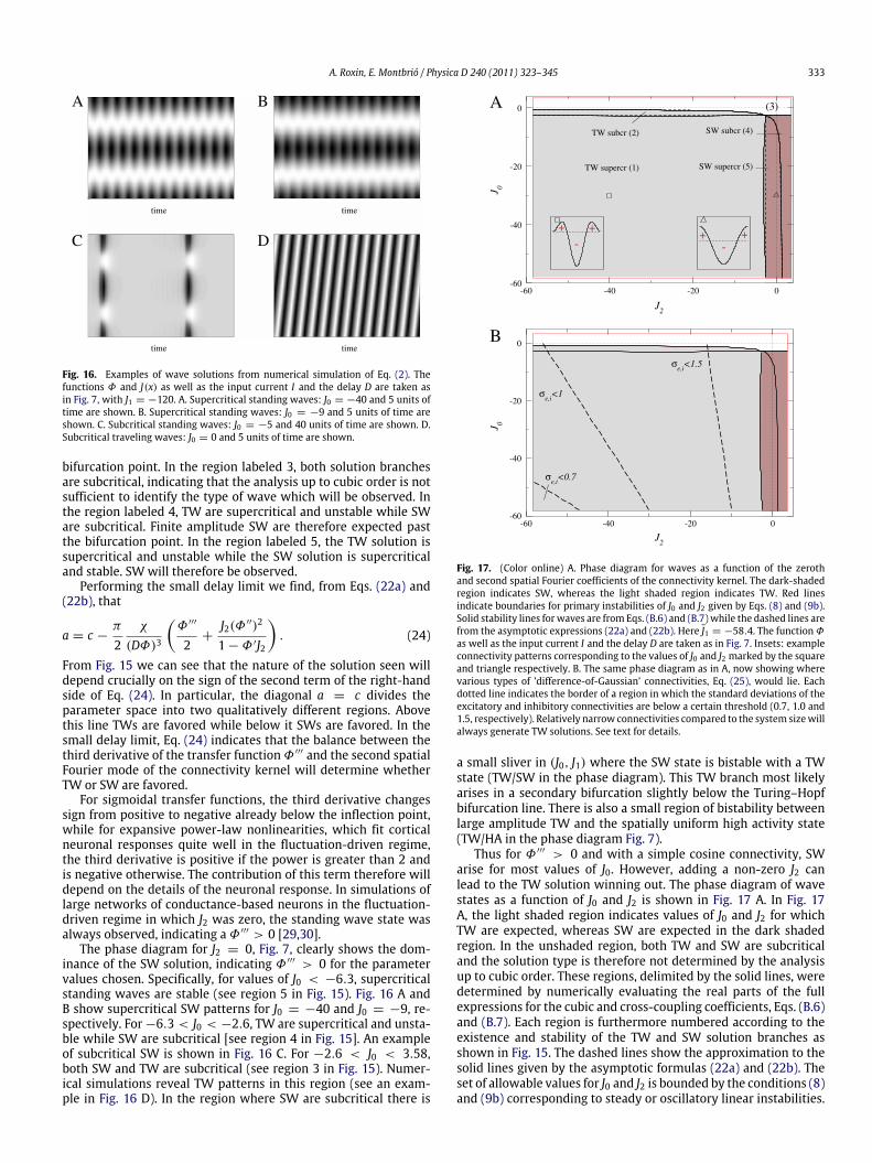
For sigmoidal transfer functions, the third derivative changessign from positive to negative already below the inflection point,while for expansive power-law nonlinearities, which fit corticalneuronal responses quite well in the fluctuation-driven regime,the third derivative is positive if the power is greater than 2 andis negative otherwise. The contribution of this term therefore willdepend on the details of the neuronal response. In simulations oflarge networks of conductance-based neurons in the fluctuation-driven regime in which J2 was zero, the standing wave state wasalways observed, indicating aΦ ′′′ > 0 [29,30].

The phase diagram for J2 = 0, Fig. 7, clearly shows the dom-inance of the SW solution, indicating Φ ′′′ > 0 for the parametervalues chosen. Specifically, for values of J0 < −6.3, supercriticalstanding waves are stable (see region 5 in Fig. 15). Fig. 16 A andB show supercritical SW patterns for J0 = −40 and J0 = −9, re-spectively. For −6.3 < J0 < −2.6, TW are supercritical and unsta-ble while SW are subcritical [see region 4 in Fig. 15]. An exampleof subcritical SW is shown in Fig. 16 C. For −2.6 < J0 < 3.58,both SW and TW are subcritical (see region 3 in Fig. 15). Numer-ical simulations reveal TW patterns in this region (see an exam-ple in Fig. 16 D). In the region where SW are subcritical there is

J2

-60

-40

-20

0

J 0

--++

+ +

(3)

J2

0

J 0

σe,i

<0.7

σe,i

<1

σe,i

<1.5

SW subcr (4)

SW supercr (5)

-60 -40 -20 0

-60

-40

-20

-60 -40 -20 0

TW supercr (1)

TW subcr (2)

A

B

Fig. 17. (Color online) A. Phase diagram for waves as a function of the zerothand second spatial Fourier coefficients of the connectivity kernel. The dark-shadedregion indicates SW, whereas the light shaded region indicates TW. Red linesindicate boundaries for primary instabilities of J0 and J2 given by Eqs. (8) and (9b).Solid stability lines forwaves are from Eqs. (B.6) and (B.7) while the dashed lines arefrom the asymptotic expressions (22a) and (22b). Here J1 = −58.4. The functionΦas well as the input current I and the delay D are taken as in Fig. 7. Insets: exampleconnectivity patterns corresponding to the values of J0 and J2 marked by the squareand triangle respectively. B. The same phase diagram as in A, now showing wherevarious types of ’difference-of-Gaussian’ connectivities, Eq. (25), would lie. Eachdotted line indicates the border of a region in which the standard deviations of theexcitatory and inhibitory connectivities are below a certain threshold (0.7, 1.0 and1.5, respectively). Relatively narrow connectivities compared to the system sizewillalways generate TW solutions. See text for details.

a small sliver in (J0, J1) where the SW state is bistable with a TWstate (TW/SW in the phase diagram). This TW branch most likelyarises in a secondary bifurcation slightly below the Turing–Hopfbifurcation line. There is also a small region of bistability betweenlarge amplitude TW and the spatially uniform high activity state(TW/HA in the phase diagram Fig. 7).

Thus for Φ ′′′ > 0 and with a simple cosine connectivity, SWarise for most values of J0. However, adding a non-zero J2 canlead to the TW solution winning out. The phase diagram of wavestates as a function of J0 and J2 is shown in Fig. 17 A. In Fig. 17A, the light shaded region indicates values of J0 and J2 for whichTW are expected, whereas SW are expected in the dark shadedregion. In the unshaded region, both TW and SW are subcriticaland the solution type is therefore not determined by the analysisup to cubic order. These regions, delimited by the solid lines, weredetermined by numerically evaluating the real parts of the fullexpressions for the cubic and cross-coupling coefficients, Eqs. (B.6)and (B.7). Each region is furthermore numbered according to theexistence and stability of the TW and SW solution branches asshown in Fig. 15. The dashed lines show the approximation to thesolid lines given by the asymptotic formulas (22a) and (22b). Theset of allowable values for J0 and J2 is bounded by the conditions (8)and (9b) corresponding to steady or oscillatory linear instabilities.

334 A. Roxin, E. Montbrió / Physica D 240 (2011) 323–345

These stability conditions are shown by the horizontal and verticalbounding lines (red online). All parameter values are as in Fig. 7.

From Fig. 17 we can now understand the discrepancy betweenthe analytical results in [29] using a rate equation with a linearthreshold transfer function, which predicted TW, and networksimulations, which showed SW. Specifically, given a nonlineartransfer function withΦ ′′′ > 0, thenwith a simple cosine couplingSW are predicted over almost the entire range of allowable J0(dark shaded region for J2 = 0). The nonlinear transformation ofinputs into outputs is thus crucial in determining the type of wavesolution. The choice of a threshold linear transfer function resultsin the second and all higher order derivatives being zero. In thissense it produces degenerate behavior at a bifurcation point, andby continuation of the solution branches, in a finite region of thephase diagram.

4.3.4. ‘Difference-of-Gaussian’ connectivitiesWe have shown that varying J0 can change the nature of the

bifurcation, e.g. supercritical to subcritical, while varying J2 canswitch the solution type, e.g. from SW to TW. As an example of afunctional form of connectivity motivated by anatomical findings,e.g. [42], we consider a difference of Gaussians, written as

J(x) =Je

√2πσe

e−

x2

2σ2e −Ji

√2πσi

e−

x2

2σ2i . (25)

In this case, one finds that the Fourier coefficients are

Jk = Jee−k2σ 2e /2f (k, σe)− Jie−k2σ 2

i /2f (k, σi) (26)

where f (k, σe,i) = Re[Erf((π/σe,i + ik2)/√2)]/π . Once J1 has

been fixed at the critical value for the onset of waves, from Eq.(26) it is straightforward to show that J0 = −pJ2 + q whereboth p and q are constants which depend on σe and σi, the widthsof the excitatory and inhibitory axonal projections respectively.Thus a difference-of-Gaussian connectivity constrains the possiblevalues of J0 and J2 to lie along a straight line for fixed connectivitywidths. This is illustrated in Fig. 17B where three dashed lines aresuperimposed on the phase diagram, corresponding to the valuesσe,i = (1.5, 1.49); σe,i = (1, 0.99); and σe,i = (0.7, 0.69). Eachof these lines is bounding a region to the left where σe and σi areless than 0.7, 1.0 and 1.5 respectively. Given periodic boundaryconditions with a system size of 2π , a Gaussian with σ = 1.5is already significantly larger than zero for x = π or −π . Thus,restricting ourselves to Gaussians which essentially decay to zeroat the boundaries means that TW will always be observed. Thesame holds true for qualitatively similar types of connectivity.

4.3.5. Classes of waves in network simulationsOur analytical results concerning waves from the rate equation

Eq. (2) predict that a connectivity with a sufficiently strong secondFourier componentwith a negative amplitudewill lead to travelingwaves (see the phase diagram in Fig. 17(A)).

Here we have confirmed this prediction performing numericalsimulations of the network of spiking neurons described in theAppendix A. Indeed, Fig. 18 shows that the addition of the secondspatial Fourier component to the inhibitory connections convertsstanding waves (SW) into travelling waves (TW).

5. Bifurcations of codimension 2

For certain connectivity kernels we may be in the vicinityof two distinct instabilities. This is the case for certain Mexicanhat connectivities (OU and SB) and certain inverted Mexican hatconnectivities (OU and SW/TW). Although two instabilities willco-occur only at a single point in the phase diagram Fig. 7, i.e. J0and J1 are both at their critical values, the competition between

these instabilities may lead to solutions which persist over a broadrange of connectivities. This is the case here. We can investigatethis competition once again using a weakly nonlinear approach.The main results of this section are summarized in Table 1.

5.1. Hopf and Turing–Hopf bifurcations

Herewe consider the co-occurrence of a spatially homogeneousoscillation and a spatially inhomogeneous oscillation (OU andSW/TW), both with frequency ω given by Eq. (9a). This instabilityoccurs when the zeroth and kth spatial Fourier mode of theconnectivity both satisfy the relation, Eq. (9b), while we assumethat all other Fourier modes are sufficiently below their criticalvalues to avoid additional instabilities. Without loss of generalitywe take k = 1 for the SW/TW state.

We expand the parameters J0, J1, I and r as in Eqs. (12)–(14),and define the slow time (15). The linear solution consistsof homogeneous, global oscillations, leftwards and rightwardstraveling waves with amplitudes which we allow to vary slowly intime, i.e. r1 = H(T )eiωt +A(T )eiωt+ix

+ B(T )e−iωt+ix+ c.c. Carrying

out a weakly nonlinear analysis to third order in ϵ leads to thecoupled amplitude equations

∂TH = (µ+ iΩ)∆J0H

+ 2(α + iβ)[

|H|2

2+ |A|

2+ |B|2

H + H∗AB∗

], (27a)

∂TA = (µ+ iΩ)∆J1A + (a + ib)|A|2A + (c + id)|B|2A

+ (α + iβ)[2|H|2A + H2B], (27b)

∂TB = (µ− iΩ)∆J1B + (a − ib)|B|2B + (c − id)|A|2B

+ (α − iβ)[2|H|2B + H∗2A], (27c)

where α + iβ , a + ib and c + id are given by Eqs. (B.5)–(B.7),respectively. The overbar in H∗ represents the complex conjugate.

5.1.1. Solution types and their stabilityEqs. (27a)–(27c) admit several types of steady state solutions

including oscillatory uniform solutions (OU), travelingwaves (TW),standingwaves (SW) andmixedmode oscillations/standingwaves(OU–SW). The stability of these solutions depends on the valuesof the coefficients in Eqs. (27a)–(27c). In addition, non-stationarysolutions are also possible. Here we describe briefly somestationary solutions and their stability. For details see Appendix B.Oscillatory uniform (OU): the oscillatory uniform solution has theform (H, A, B) = (Heiωt , 0, 0)where

H =

−µ∆J0α

,

ω =

Ω −

βµ

α

∆J0.

The OU state undergoes a steady instability along the line

∆J1 = ∆J0. (28)

This stability line agrees very well with the results of numericalsimulations of Eq. (2) [see the phase diagram Fig. 7].Traveling waves (TW): the traveling wave solution has the form(H, A, B) = (0,ATWeiωt , 0) or (0, 0,ATWe−iωt), where

ATW =

−µ∆J1

a,

ω =

Ω −

bµa

∆J1.

The TW state undergoes an oscillatory instability along the line

∆J1 =a2α∆J0, (29)

A. Roxin, E. Montbrió / Physica D 240 (2011) 323–345 335

(A)

950

(B)

1000

neur

on in

dex

0

2000

neur

on in

dex

1000

0

2000

950

time (ms)900 1000 1000

time (ms)900

Fig. 18. The transition from (A) standing to (B) travelling waves in a network of conductance-based neurons takes place by increasing the second Fourier mode of thesynaptic connectivity pI2 . (A) p

I2 = 0, (B) pI2 = 0.1. Remaining parameters: pE,I0 = pI1 = 0.2, pE1,2 = 0, gE = 0.01, gI = 0.028, gext = 0.001 mS ms/cm2 , and νext = 5000 Hz.

Table 1Some existing dynamical states that are present close to the codimension-2 bifurcations, and their corresponding instability boundaries Eqs. (28), (29), (32), (33), (39) and(40), except for the Mixed Mode solutions.

Codim.-2 bifurcations Solution types calculated Instability boundaries

Hopf and Turing–Hopf Oscillatory uniform ∆J1 = ∆J0Travelling waves ∆J1 = a/(2α)∆J0Standing waves (osc.) ∆J1 = (a + c)/(4α)∆J0Standing waves (stat.) ∆J1 = Ψ∆J0Mixed-mode Not calculated

Hopf and Turing Oscillatory uniform ∆J1 = (µσ)/(ηα)∆J0Stationary bump ∆J1 = (µΓ )/(ηκ)∆J0Mixed-mode (OU–SB) Not calculated

with a frequency

ω =

Ω

1 −

a2α

+ (b − 2β)

µ

2α

∆J0.

Standing waves (SW): the standing wave solution has the form(H, A, B) = (0,ASWeiωt ,ASWe−iωt), where

ASW =

−µ∆J1(a + c)

, (30)

ω =

Ω −

(b + d)(a + c)

µ

∆J1. (31)

An oscillatory instability occurs along the line

∆J1 =(a + c)

4α∆J0, (32)

with a frequency

ω =

[Ω

a + c4α

− 1

− µb + d − 4β

4α

]2− µ2 α

2 + β2

4α2∆J0.

A stationary instability occurs along the line

∆J1 = Ψ∆J0, (33)

where

Ψ =

−k2 +

k22 − 4k1k3

2k1,

k1 =

[Ω − µ

(b + d − 4β)(a + c)

]2+ µ2 (12α

2− 4β2)

(a + c)2,

k2 = −8µ2 α

(a + c)− 2Ω2

+ 2Ωµ(b + d − 4β)(a + c)

,

k3 = µ2+Ω2.

For Eq. (2) with the parameters used to generate the phasediagram Fig. 7, we find that the stationary instability precedes

the oscillatory one and that Ψ ∼ 0.6. This agrees well withthe numerically determined stability line near the co-dimension2 point in diagram Fig. 7.Mixedmode: we can study themixedmode solutions in Eqs. (27a)–(27c) by assuming an ansatz

(H, A, B) = (Heiθ ,AeiψA ,Be−iψB), (34)

which leads to four coupled equations [see (Appendix B)]. We donot study the stability of mixed mode solutions in this work.

5.1.2. A simple exampleWe now turn to a simple example in order to illustrate the

two main types of bifurcation scenarios that can arise when smallamplitude waves and oscillations interact in harmonic resonance.

i. Bistability: Here we take the parameters µ = −1, ∆J0 = −1,α = −1, a = −1, b = c = d = β = ω = Ω = 0. Given these pa-rameter values one finds, from the analysis above, that the oscilla-tory uniform state has an amplitude H = 1 and destabilizes alongthe line ∆J1 = −1. The standing wave solution (traveling wavesare unstable [see Fig. 15]) has an amplitude ASW =

√−∆J1 which

undergoes a steady bifurcation to the oscillatory uniform state at∆J1 = −1/2. Both solutions are therefore stable in the region−1 < ∆J1 < −1/2. This analysis is borne out by numerical sim-ulation of Eqs. (27a)–(27c) [see Fig. 19a]. Solid and dotted linesare the analytical expressions for the stable and unstable solutionbranches respectively (red is OU and black is SW). Circles are fromnumerical simulation of the amplitude Eqs. (27a)–(27c).

Note that this scenario is the relevant one for the phase diagramshown in Fig. 7. That is, we find there is a region of bistabilitybetween the OU and SW solutions, bounded between two lineswith slope ∼ 0.6 and 1 respectively.

ii. Mixed mode: here we consider the parameters µ = −1,∆J0 − 1, α = −1, a = −8, β = 1, b = c = d = ω =

Ω = 0. Given these parameter values one finds that the oscillatoryuniform state has an amplitude H = 1 and destabilizes along theline ∆J1 = −1. The standing waves solution has an amplitude

336 A. Roxin, E. Montbrió / Physica D 240 (2011) 323–345

ΔJ1

H

ASW

ΔJ1

H

ASW

HMM

AMMMM osc

1

0.5

0

1.5

-2 -1.5 -1 -0.5 00

0.2

0.4

0.6

0.8

1

ampl

itude

ampl

itude

-3 -2 -1 0

(A) (B)

Fig. 19. Two typical bifurcation diagrams for the case of harmonic resonance between small-amplitude oscillations and small-amplitude standingwaves. A: here oscillationsand standing waves are bistable for −1 < ∆J1 < −1/2.∆J0 = −1, α = −1, a = −1, b = c = d = β = Ω = 0, µ = −1. B: here the standing wave solution loses stabilityto an oscillatory mixed-mode solution at ∆J1 = −2. At ∆J1 ∼ −1.75 a steady mixed-mode solution arises in a saddle–node bifurcation and continuously approaches theoscillatory pure-mode solution at∆J1 = −1. Parameters are a = −8, β = 1, α = −1,µ = −1, b = c = d = Ω = 0. The phase φ of the mixed-mode solution is not shown.

ASW =√

−∆J1/8 (traveling waves are again unstable) whichundergoes an oscillatory instability at∆J1 = −2. Themixed-modesolution is given by

H =4 +∆J1(2 − cosφ − sinφ)4 − (2 − cosφ − sinφ)2

, (35a)

ASW =∆J1 + (2 − cosφ − sinφ)8 − 2(2 − cosφ − sinφ)2

, (35b)

1 = ∆J1(1 − 4 cosφ − 2 sinφ + 2 sinφ cosφ)− 4 cosφ + 8 cosφ2. (35c)

It is easy to show that for ∆J1 → −1 the mixed mode amplitudesapproach (H,ASW ) = (1, 0) and the phase φ → 0. The mixed-mode solution thus bifurcates continuously from the oscillatorypure mode. Fig. 19b shows the corresponding bifurcation diagramwhere solid and dotted lines are the analytical expressions for thesolution branches and symbols are from numerical simulation ofEqs. (27a)–(27c). As ∆J1 increase from the left we see that theSW solution indeed undergoes an oscillatory instability at ∆J1 =

−2 leading to an oscillatory mixed-mode solution indicated bysmall circles (the maximum and minimum amplitude achievedon each cycle is shown). This oscillatory solution disappears ina saddle–node bifurcation, giving rise to a steady mixed-modesolution whose amplitude is given by Eqs. (35a)–(35c). This steadymixed-mode solution bifurcates from the pure oscillatory mode at∆J1 = −1 as predicted.

5.1.3. SummaryThe interaction between the oscillatory uniform state and

waves may lead to mixed mode solutions or bistability. The OUstate always destabilizes along the line J1 = J0, irrespective ofparameter values or the choice of Φ or J(x). This result from theweakly nonlinear analysis agrees with numerical simulations ofEq. (2) over the entire range of values of J0 and J1 used in thephase diagram, Fig. 7, and appears to be exact. Depending on thevalue of J2, supercritical TW or supercritical SW will be stablenear the codimension 2 point. In the case of TW, the slope of thestability line is one half the ratio of the cubic coefficient of wavesto that of oscillations. In the small delay limit this expression canbe simplified to

a2α

∼π

4

(Φ′′)2

Φ′ −Φ′′′

2

(11π−4)

20(Φ′′)2

Φ′ −πΦ′′′

4

, (36)

which depends only on the shape of the transfer function Φ . Forthe parameter values used in the phase diagram Fig. 7 this yieldsa line with slope close to one half. Thus TW and OU are expected

Fig. 20. Bistability between SW and OU states in an inhibitory network withpI (r) = 0.4 + 0.2 cos r , where r is the distance between neurons, νext = 4500 Hz,and gI = 0.1 mS · ms/cm2 . This is the only network simulation for which anexplicit delay has been added of δ = 0.5 ms. Removing the explicit delay for theseparameter values eliminates the bistability. Parameter values are identical for bothsimulations. In the simulation shown in the bottom raster a hyperpolarizing currentof Iapp = −5.0µA/cm2 was injected into cells 1–1000 for 30ms at time t = 400ms,switching the state from OU to SW.

to be bistable in the wedge between∆J1 = ∆J0/2 and∆J1 = ∆J0.In the case of SW, the slope of the stability line is a complicatedfunction of the shape of Φ and the second Fourier coefficient J2.For the parameter values used in the phase diagram Fig. 7 the slopeis close to 0.6. Therefore the OU and SW states are bistable in thewedge between∆J1 = 0.6∆J0 and∆J1 = ∆J0.

5.1.4. Network simulationsGiven that network simulations robustly reveal standing wave

patterns, we would expect to find either mixed-mode SW–OU orbistability between SW and OU. As we have shown previously,e.g. [29], there is a region of bistability between SW and OU innetwork simulations for strongly modulated inhibitory connectiv-ity. Herewe show additional network simulations that suggest thisbistable region is in the vicinity of the codimension 2 point, i.e. itis a bistability between the OU and SW states arising via primarybifurcations of the unpatterned state.

Fig. 20 shows two rasters from simulations of a purely in-hibitory network with strongly spatially modulated connectivity.The top raster shows 300ms of activity in which homogeneous os-cillations are clearly observable. In the bottom raster, the networkis started from precisely the same initial condition, but a hyperpo-larizing input current is applied to neurons 1–1000 from t = 400to t = 430 ms. The network activity clearly switches to an SWstate in response to this input. The SW state persists for as longas simulations were carried out (10 s). The network thus exhibitsbistability between the OU and SW states.

A. Roxin, E. Montbrió / Physica D 240 (2011) 323–345 337

A C

B D

Fig. 21. Increasing the strength of recurrent excitatory connections drives the system out of the bistable regime and into an SW state. A: a raster plot of 3 s of simulation. Forthe first 500 ms the simulation is identical to that shown in the top panel of Fig. 20. Thereafter the weights of the recurrent excitatory synaptic are slowly increased whilethe external drive is slowly decreased so as to maintain stable mean firing rates. There is a spontaneous destabilization of the OU state to an SW state around t = 1500 ms.B: the network firing rate for the simulation shown in A (top), the time course of the excitatory synaptic weights (middle) and external drive (bottom). C: for the first 500msthe simulation is identical to that shown in the bottom panel of Fig. 20, i.e. there is a hyperpolarizing current injected at time t = 400 ms which switches the state from OUto SW. Thereafter the weights of recurrent excitatory synapses are slowly increased while the external drive is slowly decreased so as to maintain stable mean firing rates.D: the network firing rate and time courses of the excitatory synaptic weights and external drive, as in B.

In order to determine if this region of bistability is related tothe codimension 2 point, we adiabatically increased the recurrentexcitatory connectivity in the network, thereby mimicking anincrease in J0 in the rate model. This is done by generating anetwork of both inhibitory and excitatory neurons with pI(r) =

0.4+0.2 cos r and pE = 0.2. Theweights of the inhibitory synapsesare taken as gI = 0.1 while excitatory weights are allowed to vary.Specifically, gE = 0 for the first 500 ms of the simulation and arethen slowly increased according to gE(t) = 1.0526 ·10−5(t−500).At the same time we slowly decrease the external drive in orderto maintain mean firing rates. Thus νext = 4500 for the first500 ms and is then varied according to νext = 4500 − 0.158(t −

500) thereafter. This particular functional form was determinedempirically to keep the mean firing rates steady. Therefore, forthe first 500 ms of simulation time the network is equivalent tothat shown in Fig. 20 while at later times the network is no longerpurely inhibitory.

Carrying out such an adiabatic increase in the recurrent exci-tation should cause the network to cross the line of instability ofthe OU state, leading to stable SW. Thus, if we begin simulationsin the OU state, they should destabilize at some point to SW whileif we begin in the SW state they should persist. This is preciselywhat occurs. Fig. 21A shows a raster plot of three seconds of sim-ulation time beginning in the OU state. A transition to the SW oc-curs around 1500ms. Fig. 21B shows the network firing rate duringthese three seconds (top) as well as the time course of the excita-tory synaptic weights and external drive (middle and bottom re-spectively). Note that themean firing rate is relatively steady in theOU state indicating that the co-variation of the synaptic weights

and external drive balance one another. Fig. 21C and D analogouslyshow the raster and firing rate of a simulation inwhich the networkis switched into an SW state at t = 400 ms. Note that the SW statepersists over the whole 3 s simulation.

5.2. Hopf and Turing bifurcations

We consider the co-occurrence of two instabilities: a spatiallyhomogeneous oscillation and a spatially inhomogeneous steadysolution. This occurs when the zeroth spatial Fourier mode ofthe connectivity satisfies the relation, Eq. (9b) and the kth spatialFourier mode satisfies J1 = 1/Φ ′, while we assume that all otherFourier modes are sufficiently below their critical values to avoidadditional instabilities. Without loss of generality we take k = 1for the Turing instability.

We expand the parameters J0, J1, I and r as in Eqs. (12)–(14),and define the slow time (15). The linear solution consists ofhomogeneous, global oscillations and stationary, spatially periodicbumps with amplitudes which we allow to vary slowly in time,i.e. r1 = H(T )eiωt + A(T )eix + c.c. Carrying out a weakly nonlinearanalysis to third order in ϵ leads to the coupled amplitudeequations

∂TH = (µ+ iΩ)∆J0H + (α + iβ)|H|2H

+ (κ + iΛ)|A|2H, (37a)

∂TA = η∆J1A + Γ |A|2A + σ |H|

2A, (37b)

where µ+ iΩ , α + iβ , η, Γ , κ + iΛ and σ are given by Eqs. (B.4),(B.5), (17a), (17b), (B.15) and (B.16), respectively.

338 A. Roxin, E. Montbrió / Physica D 240 (2011) 323–345

5.2.1. Solution types and their stabilitySteady state solutions to Eqs. (37a) and (37b) include puremode

OU, pure mode SB and mixed mode solutions (OU–SB). We look atthe stability of the OU and SB solutions in turn for the general caseand then look specifically at the case of small delay in Eq. (2). Sincethe coupling in Eqs. (37a) and (37b) is only through the amplitudeswe can simplify the equations by taking (H, A) = (Heiθ ,Aeiφ)which yields

H = µ∆J0H + αH3+ κA2H, (38a)

A = η∆J1A + ΓA3+ σH2A. (38b)

Oscillatory uniform (OU): the uniform oscillations have the form(H∗, 0)where

H =

−µ∆J0α

.

The linear stability of this solution can be calculated with theansatz

(H,A) = (H∗+ δHeλt , δAeλt),

which yields the two eigenvalues

λH = −2µ∆J0,

λA = η∆J1 +µσ

α∆J0.

If we assume a supercritical uniform oscillatory state then the firsteigenvalue is always negative, while the second becomes positivealong the line

∆J1 =µσ

ηα∆J0, (39)

indicating the growth of a bump solution.For Eq. (2) with the parameters used to generate the phase di-

agram Fig. 7, we find from Eq. (39) that the OU state destabilizesalong the line∆J1 ∼ −0.026∆J0.Stationary bump (SB): the stationary bump solution has the form(0,A∗)where

A =

−η∆J1Γ

.

The linear stability of this solution can be calculated with theansatz

(H,A) = (δHeλt ,A∗+ δAeλt),

which yields the two eigenvalues

λH = µ∆J0 −ηκ

Γ∆J1,

λA = −2η∆J1.

If we assume a supercritical stationary bump state then the secondeigenvalue is always negative, while the first becomes positivealong the line

∆J1 =µΓ

ηκ∆J0, (40)

indicating the growth of uniform oscillations.For Eq. (2) with the parameters used to generate the phase

diagram7,we find fromEq. (40) that the SB state destabilizes alongthe line∆J1 ∼ −0.144∆J0.Mixed mode (OU–SB): the mixed-mode solution satisfies the fol-lowing matrix equationα κσ Γ

H2

A2

= −

µ∆J0η∆J1

,

which yields

H2=

−µΓ∆J0 + ηκ∆J1αΓ − σκ

,

A2=µσ∆J0 − ηα∆J1αΓ − σκ

.

We do not study the stability of the mixed-mode solution here.

5.2.2. A simple exampleWe once again illustrate the scenarios of bistability and mixed-

mode solutions with a simple example.i. Bistability1: in this case, the limit cycle has an amplitude

H = 1 and undergoes an instability at ∆J1 = 2. The bumpsolution has an amplitude A =

√∆J1 and becomes unstable

at ∆J1 = 1/2. The oscillatory and bump solutions are thereforebistable in the range 1/2 < ∆J1 < 2. This is borne out in numericalsimulations of Eqs. (38a) and (38b) [see Fig. 22A]. Symbols are fromnumerical simulation (circles:limit cycle, squares:bump), whilelines are analytical solutions.

ii. Mixed-mode2: in this case, the limit cycle has an amplitudeH = 1 and undergoes an instability at ∆J1 = 1/2. The bumpsolution has an amplitude A =

√∆J1 and becomes unstable at

∆J1 = 2. The mixed-mode solution is stable in the range 1/2 <∆J1 < 2 and has amplitudes HMM = 2

√(1 −∆J1/2)/3 and

A = 2√(∆J1 − 1/2)3. The corresponding bifurcation diagram is

shown in Fig. 22B where symbols are from simulation of Eqs. (38a)and (38b) and lines are the analytical results.

5.2.3. SummaryThe interaction between the SB and OU states can lead to one

of two scenarios. Either there is a region of bistability betweenbumps and oscillations, or there is a mixed-mode solution which,near the codimension-2 point at least, will consist of bumpswhoseamplitude oscillates in time, i.e. oscillating bumps (OB).

In the limit of small D the instability lines for the OU and SBstates in the vicinity of the codimension 2 point are given by theequations

∆J1 = −D

(Φ′′)

2

Φ′ − Φ ′′′

(11π−4)

20(Φ′′)2

Φ′ − π Φ′′′

4

∆J0, (41)

∆J1 = −2πD

(Φ′′)2

Φ′ −Φ′′′

2 −J2(Φ′′)2

2(1−J2Φ′)

(Φ′′)2

Φ′ − Φ ′′′

∆J0. (42)

respectively. The slope of both of the stability lines is proportionalto D, indicating that in the small D limit any region of bistabilityor mixed mode solution will be limited to a narrowwedge close tothe J0 axis. Which scenario will be observed (bistability or mixed-mode) depends on the particular choice of Φ ′ and the value ofthe second spatial Fourier mode of the connectivity J2. For theparameter values used to generate the phase diagram Fig. 7 theslopes are ∼−0.026 and ∼−0.144 for the OU and SB stability linesrespectively, indicating a mixed mode solution.

5.2.4. Network simulationsAs shown in [29], oscillating bump solutions can be found in

networks of spiking neurons with Mexican-hat connectivity andstrong inhibition. Here we have identified such oscillating bumpsas arising via a bifurcation tomixed-modeOU and SB in the vicinity

1 µ = α = Γ = ∆J0 = −1, σ = κ = −2.2 µ = α = Γ = ∆J0 = −1, σ = κ = −1/2.

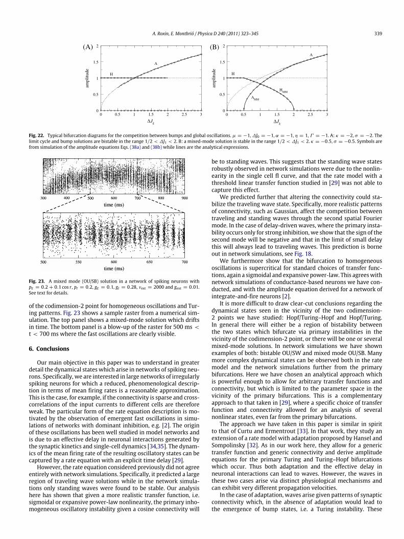
A. Roxin, E. Montbrió / Physica D 240 (2011) 323–345 339

ΔJk

(A)

A

H

ΔJk

(B)A

H

HMM

AMM

0.5

1

1.5

0.5

1

1.5

ampl

itude

0

2

ampl

itude

0

2

0 0.5 1 1.5 2 2.5 3 0 0.5 1 1.5 2 2.5 3

Fig. 22. Typical bifurcation diagrams for the competition between bumps and global oscillations. µ = −1,∆J0 = −1, α = −1, η = 1, Γ = −1. A: κ = −2, σ = −2. Thelimit cycle and bump solutions are bistable in the range 1/2 < ∆J1 < 2. B: a mixed-mode solution is stable in the range 1/2 < ∆J1 < 2. κ = −0.5, σ = −0.5. Symbols arefrom simulation of the amplitude equations Eqs. (38a) and (38b) while lines are the analytical expressions.

Fig. 23. A mixed mode (OU/SB) solution in a network of spiking neurons withpE = 0.2 + 0.1 cos r , pI = 0.2, gE = 0.1, gI = 0.28, νext = 2000 and gext = 0.01.See text for details.

of the codimension-2 point for homogeneous oscillations and Tur-ing patterns. Fig. 23 shows a sample raster from a numerical sim-ulation. The top panel shows a mixed-mode solution which driftsin time. The bottom panel is a blow-up of the raster for 500 ms <t < 700 ms where the fast oscillations are clearly visible.

6. Conclusions

Our main objective in this paper was to understand in greaterdetail the dynamical states which arise in networks of spiking neu-rons. Specifically, we are interested in large networks of irregularlyspiking neurons for which a reduced, phenomenological descrip-tion in terms of mean firing rates is a reasonable approximation.This is the case, for example, if the connectivity is sparse and cross-correlations of the input currents to different cells are thereforeweak. The particular form of the rate equation description is mo-tivated by the observation of emergent fast oscillations in simu-lations of networks with dominant inhibition, e.g. [2]. The originof these oscillations has been well studied in model networks andis due to an effective delay in neuronal interactions generated bythe synaptic kinetics and single-cell dynamics [34,35]. The dynam-ics of the mean firing rate of the resulting oscillatory states can becaptured by a rate equation with an explicit time delay [29].

However, the rate equation considered previously did not agreeentirely with network simulations. Specifically, it predicted a largeregion of traveling wave solutions while in the network simula-tions only standing waves were found to be stable. Our analysishere has shown that given a more realistic transfer function, i.e.sigmoidal or expansive power-law nonlinearity, the primary inho-mogeneous oscillatory instability given a cosine connectivity will

be to standing waves. This suggests that the standing wave statesrobustly observed in network simulations were due to the nonlin-earity in the single cell fI curve, and that the rate model with athreshold linear transfer function studied in [29] was not able tocapture this effect.

We predicted further that altering the connectivity could sta-bilize the traveling wave state. Specifically, more realistic patternsof connectivity, such as Gaussian, affect the competition betweentraveling and standing waves through the second spatial Fouriermode. In the case of delay-driven waves, where the primary insta-bility occurs only for strong inhibition, we show that the sign of thesecond mode will be negative and that in the limit of small delaythis will always lead to traveling waves. This prediction is borneout in network simulations, see Fig. 18.

We furthermore show that the bifurcation to homogeneousoscillations is supercritical for standard choices of transfer func-tions, again a sigmoidal and expansive power-law. This agreeswithnetwork simulations of conductance-based neurons we have con-ducted, and with the amplitude equation derived for a network ofintegrate-and-fire neurons [2].

It is more difficult to draw clear-cut conclusions regarding thedynamical states seen in the vicinity of the two codimension-2 points we have studied: Hopf/Turing–Hopf and Hopf/Turing.In general there will either be a region of bistability betweenthe two states which bifurcate via primary instabilities in thevicinity of the codimension-2 point, or there will be one or severalmixed-mode solutions. In network simulations we have shownexamples of both: bistable OU/SW and mixed mode OU/SB. Manymore complex dynamical states can be observed both in the ratemodel and the network simulations further from the primarybifurcations. Here we have chosen an analytical approach whichis powerful enough to allow for arbitrary transfer functions andconnectivity, but which is limited to the parameter space in thevicinity of the primary bifurcations. This is a complementaryapproach to that taken in [29], where a specific choice of transferfunction and connectivity allowed for an analysis of severalnonlinear states, even far from the primary bifurcations.

The approach we have taken in this paper is similar in spiritto that of Curtu and Ermentrout [33]. In that work, they study anextension of a rate model with adaptation proposed by Hansel andSompolinsky [32]. As in our work here, they allow for a generictransfer function and generic connectivity and derive amplitudeequations for the primary Turing and Turing–Hopf bifurcationswhich occur. Thus both adaptation and the effective delay inneuronal interactions can lead to waves. However, the waves inthese two cases arise via distinct physiological mechanisms andcan exhibit very different propagation velocities.

In the case of adaptation, waves arise given patterns of synapticconnectivity which, in the absence of adaptation would lead tothe emergence of bump states, i.e. a Turing instability. These

340 A. Roxin, E. Montbrió / Physica D 240 (2011) 323–345

tend to be Mexican-hat like connectivities. In the presence ofadaptation, stationary bump states may destabilize since the peakof activity is preferentially suppressed compared to activity atthe edge of the bump. As a result the bump begins to move viaa symmetry-breaking bifurcation, generally leading to travelingwaves. This only occurs if the adaptation is significantly strong,i.e. above a critical threshold. In a two-population model withadaptation studied in [33], the frequency of the waves was shownto be proportional to the square root of the difference betweenthe strength of adaptation and a critical value below which nobifurcation is possible. Thus the resulting waves can be arbitrarilyslow depending on the strength of adaptation.

In the case of rate equations with delay, a Turing–Hopf insta-bility occurs only for connectivities which are strongly inhibitorylocally, i.e. inverted Mexican-hat connectivities. A transient per-turbation which increases the firing rate locally will, after a delay,strongly self-inhibit while increasing the firing rate ofmore distantneurons. The process then repeats, leading to a propagation of ac-tivity. The frequency of such waves is clearly related to the delay,which itself depends on the synaptic time constants as well as thespike generation currents [34,35].

Finally, we have tried to emphasize the importance of fixeddelays in shaping the dynamics described by Eq. (2) and byextension in networks of spiking neurons. Nonetheless both fixedand conduction delays are present in neuronal systems and areroughly of the same order of magnitude in a small patch of cortexof ∼1 mm in extent. It remains to be studied how these delaysinteract to shape patterns of spontaneous activity.

Acknowledgement

EM acknowledges the financial support provided by the Centrede Recerca Matemàtica (CRM), 08193 Bellaterra, Barcelona, Spain.

Appendix A. The network of spiking neurons

In this appendix we describe the network of conductance-based neurons used in simulations. The single cell model is takenfrom [43]. The network consists of two populations of neurons:one excitatory and one inhibitory. The number of neurons in eachpopulation is NE and NI respectively. The membrane voltage of theith neuron in the excitatory population evolves according to thedifferential equation

CmVi = −INa,i − IK ,i − IL,i − Isyn,i + Iapp,i,

where themembrane capacitance Cm = 1µF/cm2 and the appliedcurrent Iapp,i have the units µA/cm2.

The leak current is

IL,i = gL(Vi − EL),

where gL = 0.1mS/cm2. Action potential generation is dependenton a sodium and a potassium current.

The sodium current is

INa,i = gNam3∞,ihi(Vi − ENa),

where gNa = 35 mS/cm2, ENa = 55 mV and the activationvariable m is assumed fast and therefore taken at its equilibriumvalue m∞,i = αm,i/(αm,i + βm,i), where αm,i = −0.1(Vi +

35)/(exp(−0.1(Vi + 35))− 1) and βm,i = 4 exp(−(Vi + 60)/18).The inactivation variable hi follows the first order kinetics

hi = φ(αh,i(1 − hi)− βh,ihi),

where φ = 5, αh,i = 0.07 exp(−(Vi + 58)/20) and βh,i =

(exp(−0.1(Vi + 28))+ 1)−1.

The potassium current is

IK ,i = gKn4i (Vi − Ek),

where gK = 9 mS/cm2 and EK = −90 mV. The activation variableni follows the first order kinetics

ni = φ(αn,i(1 − ni)− βn,ini)

where φ = 5, αn,i = −0.01(Vi + 34)/(exp(−0.1(Vi + 34)) − 1)and βn,i = 0.125 exp(−(Vi + 44)/80).

The synaptic current is

Isyn,i = gEEsE,i(t)(Vi − Esyn,E)+ gEIsI,i(t)(Vi − Esyn,I)+ gextsext,i(t)(Vi − Esyn,E),

where the reversal potentials for excitatory and inhibitory syna-pses are Esyn,E = 0 and Esyn,I = −80 respectively. The conductancechange from the activation of recurrent excitatory connections isgiven by gEEsE,i(t)where

τE,2sE,i = −sE,i + xE,i,

τE,1xE,i = −xE,i +NE−j=1

wij

−k

δ(t − tkj ), (A.1)

where the wijs ∈ 0, 1 indicate the presence or absence of asynaptic contact from cell j to cell i. The double sum in Eq. (A.1) isover all neurons in the excitatory population and over all spikes, i.e.tkj is the time of the kth spike of neuron j which will cause a jumpof amplitude 1/τE,1 in the variable xi of neuron i if wij = 1. Theresulting post-synaptic conductance change in cell i from a singlepresynaptic spike at time t∗ is given by

gEEsE,i(t) =gEE

τE,2 − τE,1(e−(t−t∗)/τE,2 − e−(t−t∗)/τE,1),

which has units of mS/cm2. The time course is therefore a dif-ference of exponentials with a rise time given by τE,1 and a de-cay time τE,2. Note that the time integral of the response sE,i fromt = t∗ to t = ∞ has been normalized to 1 and so gEE has units ofmS · ms/cm2. The synaptic current from inhibitory connections isanalogous, with time constants τI,1 and τI,2.

Finally, external inputs have the same functional form as the re-current excitatory inputs. External presynaptic spikes to excitatorycells are modeled as a Poisson process with rate νE,ext. The Poissonprocess is independent from cell to cell. Unless otherwise noted,all external inputs have weight gext = 0.0019 mS · ms/cm2, andsynpatic time constants are taken to be τ1 = 1 ms and τ2 = 3 ms.

Inhibitory neurons are modeled analogously to excitatory ones.For this work, we take all single cell parameters to be identical tothe excitatory cells. Synaptic time constants are taken to be thesame, i.e. τE,1 = τI,1 = τ1 and τE,2 = τI,2 = τ2. In additionwe take gEE = gIE = gE and gII = gEI = gI . Thus excitatoryand inhibitory synapses have identical time courses but may havedifferent strengths.

A.1. Connectivity

We choose a prescription for choosing wijs which leads tosparse, random connectivity which is spatially modulated. We dothis by defining a probability for a connection to be made from cellj in population β ∈ E, I to a cell i in population α ∈ E, I of theform

pαβ(i, j) = pαβ0 + pαβ1 cos r + pαβ2 cos 2r, (A.2)

where r is the distance between cells i and jwhich are situated on aring, normalized such that r ∈ −π, π. In order to compare withthe rate model we choose pEEl = pIE = pE and pIIl = pEIl = pIl wherel ∈ 0, 1, 2.

A. Roxin, E. Montbrió / Physica D 240 (2011) 323–345 341

Appendix B. Amplitude equations

In this appendix we outline the calculation of the amplitudeequations which describe the slow temporal evolution of thevarious instabilities near their respective bifurcations.

B.1. General framework for the weakly nonlinear calculation: codi-mension 1 bifurcations

Here we briefly describe the general framework for the weaklynonlinear calculation for the Turing, Hopf and Turing–Hopf bifur-cations.Weuse the standardmultiple-scales approachwhich takesadvantage of the fact there is a near-zero eigenvalue in the vicinityof a bifurcation which is responsible for the slow temporal evolu-tion of the critical eigenmode (see e.g. [44]).

For simplicity we first rewrite Eq. (2) as

r = −r + Φ(⟨Jr⟩ + I), (B.1)

where ⟨fg⟩ ≡12π

π−π

dyf (y− x)g(y, t − D). We study the stabilityof the steady state solution R = Φ(J0R + I), where J(x) = J0 +

2∑

∞

n=1 Jn cos nx. We expand the rates, the connectivity and theinput current as

r(x, t) = R + ϵr1(x, t, T )+ ϵr2(x, t, T )+ · · · ,

J(x) = J(x)+ ϵ2∆J(x),I = I + ϵ2∆I,

where the small parameter ϵ is defined by the distance from thecritical value of the connectivity, given by Eqs. (9a) and (9b). Plug-ging these expansions into Eq. (B.1) yields

(L + ϵ2L2)(ϵr1 + ϵ2r2 + · · ·) = ϵ2N2(r1)+ ϵ3N3(r1, r2),

where

Lr = ∂t r + r − ⟨J r⟩,L2r = ∂T ⟨J r⟩ − ⟨∆Jr⟩,

N2 =Φ ′′

2⟨J r1⟩2,

N3 = Φ ′′⟨J r1⟩⟨J r2⟩ +

Φ ′′′

6⟨J r1⟩3.

We now collect terms by order in ϵ. At first order we have

ϑ(ϵ) : Lr1 = 0.

This equation gives the linear dispersion relation equations (7). Thevalues of the connectivity and input current for which it is satisfiedare J(x) = J(x) and I = I . At second order we obtain

ϑ(ϵ2) : Lr2 = N2(r1).

The second order solution r2 is the particular solution of this lineardifferential equation. And finally, at third order

ϑ(ϵ3) : Lr3 = N3(r1, r2)− L2r1.

At this order secular terms arise which have the same temporaland/or spatial frequency as the linear solution. In order for theabove equation to have a solution, these terms must therefore beeliminated, yielding the desired amplitude equation for the insta-bility.

B.1.1. Steady bifurcation: ω = 0, k = 0For completeness we include here the derivation of the

amplitude equation for the transcritical bifurcation (see Figs. B.24and B.25).

The 0th spatial Fourier mode of the connectivity is given bythe critical value J0 =

1Φ′ , while we assume that all other

J0

R

NumericsNewton-RaphsonAmplitude eqs.

0 1 2 3 4 50

1

Fig. B.24. (Color online) Bifurcation diagram for the steady instability. Open circles:numerical simulation of Eq. (2). Red lines: amplitude equation solution from Eq.(B.3). Black lines: steady-state solution of Eq. (2) using a Newton–Raphson solver.Solid lines indicate stable solutions and dotted lines unstable ones. Φ(x) =

α

1+e−βx

where α = 1.5 and β = 3. J(x) = J0 + J1 cos x where J1 = 0. The input current I isvaried so as to keep the uniform stationary solution fixed at R = 0.1.

-a

D

-c

1

100

10000

1e+06

1

100

10000

1e+06

0 0.2 0.4 0.6 0.8 1

Fig. B.25. Top: the real part of the cubic coefficient at the codimension-2 point. Thesolid line is the full expression, Eq. (B.6) and the dotted line is the asymptotic resultin the D → 0 limit, Eq. (B.8). Bottom: the real part of the cross-coupling coefficientat the codimension-2 point. The solid line is the full expression, Eq. (B.7) and thedotted line is the asymptotic results in the D → 0 limit, Eq. (B.9).

Fourier modes are sufficiently below their critical values to avoidadditional instabilities. We expand

J0 = J0 + ϵ∆J0, (B.2)I = I + ϵ∆I,r = R + ϵr1 + ϵ2r2 + · · · ,

where the small parameter ϵ is defined by Eq. (B.2). We define theslow time T = ϵt . The linear solution is a spatially homogeneousamplitude which we allow to vary slowly in time, i.e. r1 = A(T ).Carrying out a weakly nonlinear analysis to second order in ϵ leadsto the normal form for a transcritical bifurcation given by∂TA = η∆J0A + γ A2,

η =Φ ′

1 + D,

γ =Φ ′′

2(1 + D)J20 . (B.3)

B.1.2. Turing bifurcationϑ(ϵ): the solution to the linear equation is spatially periodic

with slowly varying amplitude A,r1 = A(T )eix + c.c.

342 A. Roxin, E. Montbrió / Physica D 240 (2011) 323–345

ϑ(ϵ2): the nonlinear forcing and resulting second order solutionare

N2 = Φ ′′J21 (A2e2ix + c.c. + 2|A|

2)/2,

r2 = r22e2ix + c.c. + r20,

r22 =Φ ′′J21

2(1 − J2Φ ′)A2,

r20 =Φ ′′J21

1 − J0Φ ′|A|

2.

ϑ(ϵ3): the nonlinear forcing at cubic order is

N3 = (Φ ′′J1J0Ar20 + Φ ′′J1J2A∗r22 + Φ ′′′J31 |A|2A/2)eix + c.c. + · · · .

Eliminating all terms of periodicity eix at this order yields theamplitude equation, Eq. (16).

∂TA = η∆J1A + Γ |A|2A,

with the coefficients

η =Φ ′

1 + D,

Γ =J3k

1 + D

J0(Φ ′′)2

1 − J0Φ ′+

J2(Φ ′′)2

2(1 − J2Φ ′)+Φ ′′′

2

.

B.1.3. Hopf bifurcationϑ(ϵ): the solution to the linear equation is a time periodic func-

tion with slowly varying amplitude H

r1 = H(T )eiωt + c.c.

ϑ(ϵ2): the nonlinear forcing and resulting second order solutionare

N2 = Φ ′′J20 (H2e2iω(t−D)

+ c.c. + 2|H|2)/2,

r2 = r22e2iωt + c.c. + r20,

r22 =Φ ′′J20

2(2iω + 1 − Φ ′J0e−2iωD)e−2iωDH2,

r20 =Φ ′′J20

1 − J0Φ ′|H|

2.

ϑ(ϵ3): the nonlinear forcing at cubic order is

N3 = (Φ ′′J20Hr20 + Φ ′′J20H∗r22

+Φ ′′′J30 |A|2A/2)eiω(t−D)

+ c.c. + · · ·

Eliminating all terms of periodicity eiωt at this order yields the am-plitude equation, Eq. (18).

∂TH = (µ+ iΩ)∆J0H + (α + iβ)|H|2H,

with the coefficients

µ+ iΩ =Φ ′e−iωD

1 + D(1 + iω), (B.4)

α + iβ =e−iωD

1 + D(1 + iω)

×

J40 (Φ

′′)2

1 − Φ ′ J0+

J40 (Φ′′)2e−2iωD

2(2iω + 1 − Φ ′ J0e−2iωD)+

J30Φ′′′

2

. (B.5)

B.1.4. Turing–Hopf bifurcationϑ(ϵ): the solution to the linear equation are two sets of periodic

waves, one left-traveling with slowly varying amplitude A and the

other right-traveling with slowly varying amplitude B

r1 = A(T )eiωt+ix+ B(T )e−iωt+ix

+ c.c.= A(T )eψ + B(T )eφ + c.c.

ϑ(ϵ2): the nonlinear forcing and resulting second order solutionare

N2 = Φ ′′J21 [A2e2ψ−2iωD

+ 2ABeψ+φ+ 2AB∗eψ+φ∗

−2iωD

+ B2e2φ+2iωD+ c.c. + 2(|A|

2+ |B|2)]/2,

r2 = r2ψe2ψ + rψφeψ+φ+ rψφ∗eψ+φ∗

+ r2φe2φ + c.c. + r20,

r2ψ =Φ ′′J21

2(2iω + 1 − Φ ′J2e−2iωD)e−2iωDA2,

rψφ =Φ ′′J21

1 − Φ ′J2AB,

rψφ∗ =Φ ′′J21

2iω + 1 − J0Φ ′e−2iωDe−2iωDAB∗,

r2φ =Φ ′′J21

2(−2iωD + 1 − J2Φ ′e2iωD)e2iωDB2,

r20 =Φ ′′J21 (|A|

2+ |B|2)

1 − J0Φ ′.

ϑ(ϵ3): the nonlinear forcing at cubic order is

N3 = [Φ ′′J1(J0Ar20 + J2A∗r2ψ + J0Brψφ∗ + J2B∗rψφ)

+Φ ′′′(|A|2A/2 + |B|2A)]eψ−iωD

+ [Φ ′′J1(J0Ar∗ψφ∗ + J2A∗rψφ + J0Br20 + J2B∗r2φ)

+Φ ′′′(|B|2B/2 + |A|2B)]eφ+iωD

+ · · · .

Eliminating all terms with dependencies eiψ and eiφ yields the twocoupled amplitudes Eqs. (21a) and (21b):

∂TA = (µ+ iΩ)∆J1A + (a + ib)|A|2A + (c + id)|B|2A,

∂TB = (µ− iΩ)∆J1B + (a − ib)|B|2B + (c − id)|A|2B,

with the coefficients

a + ib =J3k e

−iωD

1 + DΦ ′ Jke−iωD

J0(Φ ′′)2

1 − Φ ′J0

+J2(Φ ′′)2e−2iωD

2(2iω + 1 − Φ ′J2e−2iωD)+Φ ′′′

2

, (B.6)

c + id =J3k e

−iωD

1 + DΦ ′ Jke−iωD

J0(Φ ′′)2

1 − Φ ′J0

+J0(Φ ′′)2e−2iωD

2iω + 1 − Φ ′J0e−2iωD+

J2(Φ ′′)2

1 − Φ ′J2+ Φ ′′′

. (B.7)

B.2. Codimension 2 bifurcations

B.2.1. Double zero eigenvalue: Hopf, Turing–Hopfϑ(ϵ): the solutions to the linear equation are periodic oscilla-

tions and traveling waves

r1 = H(T )eiωt + A(T )eψ + B(T )eφ + c.c.

where we have defined ψ ≡ i(kx + ωt) and φ ≡ i(kx − ωt).ϑ(ϵ2): the nonlinear forcing and resulting second order solu-

tion are

N2 = Φ ′′J20 (H2e2iω(t−D)

+ c.c. + 2|H|2)/2

+Φ ′′J21 [A2e2ψ−2iωD

+ 2ABeψ+φ+ 2AB∗eψ+φ∗

−2iωD

+ B2e2φ+2iωD+ c.c. + 2(|A|

2+ |B|2)]/2

+Φ ′′J0J1(HAe2iω(t−D)+ix+ H∗Be−2iω(t−D)+ix

+ AH∗eix + HBeix + c.c.),

A. Roxin, E. Montbrió / Physica D 240 (2011) 323–345 343

r2 = r22e2iωt + r2ψe2ψ + rψφeψ+φ+ rψφ∗eψ+φ∗

+ r2φe2φ

+ rHAe2iωt+ix+ rBH∗e−2iωt+ix

+ rAH∗eix + rHBeix + c.c. + r20,

rHA =Φ ′′J0J1

2iω + 1 − Φ ′J1e−2iωDe−2iωDHA,

rBH∗ =Φ ′′J0J1

−2iω + 1 − Φ ′J1e2iωDe2iωDBH∗,

rAH∗ =Φ ′′J0J1

1 − Φ ′J1AH∗,

rHB =Φ ′′J0J1

1 − Φ ′J1HB,

r20 =Φ ′′(J20 |H|

2+ J21 |A|

2+ J21 |B|

2)

1 − J0Φ ′.

ϑ(ϵ3): the nonlinear forcing at cubic order is

N3 = [Φ ′′J20 (Hr20 + H∗r22)+ Φ ′′J21 (Ar∗AH∗ + A∗rHA

+ B∗rAH∗ + Br∗BH∗ + Ar∗

HB + B∗rHB)+Φ ′′′J30 |H|

2H/2]eiω(t−D)+ [Φ ′′J1(J0Ar20 + J2A∗r2ψ

+ J0Brψφ∗ + J2B∗rψφ + J0(HrAH∗ + HrHB + H∗rHA))

+Φ ′′′(|A|2A/2 + |B|2A)]eψ−iωD

+ [Φ ′′J1(J0Ar∗ψφ∗

+ J2A∗rψφ + J0Br20 + J2B∗r2φ)+ J0(HrBH∗ + H∗rAH∗

+H∗rHB)+ Φ ′′′(|B|2B/2 + |A|2B)]eφ+iωD

+ · · · .

Eliminating terms with dependencies eiωt , eiψ and eiφ yields thethree coupled amplitudes Eqs. (27a)–(27c):

∂TH = (µ+ iΩ)∆J0H + 2(α + iβ)

×

[|H|

2

2+ |A|

2+ |B|2

H + AH∗B∗

],

∂TA = (µ+ iΩ)∆J1A + (a + ib)|A|2A + (c + id)|B|2A

+(α + iβ)(2|H|2A + H2B),

∂TB = (µ− iΩ)∆J1B + (a − ib)|B|2B + (c − id)|A|2B

+ (α − iβ)(2|H|2B + H∗2A),

where α + iβ , a + ib and c + id are given by Eqs. (B.5)–(B.7), re-spectively.

In the small delay limit (D → 0) we can use the asymptoticvalues given by Eq. (11) to obtain, to leading order,

a + ib = −χπ2 + i

(DΦ)3

(Φ ′′)2

Φ ′−Φ ′′′

2

, (B.8)

c + id = −χ

(DΦ)3

(Φ ′′)2

Φ ′

(3π − 2)5

−π

2J2(Φ ′′)2

1 − Φ ′J2−πΦ ′′′

2

+ i[(Φ ′′)2

Φ ′

(6 + π)

5−

J2(Φ ′′)2

1 − Φ ′J2− Φ ′′′

]. (B.9)

where χ ≡ π3/(8 + 2π2) and α + iβ is given by Eq. (19b).Solutions and their stabilityOscillatory uniform OU:

this solution can be expressed as (H, A, B) = (Heiωt , 0, 0),where

H =

−µ∆J0α

,

ω =

Ω −

βµ

α

∆J0.

The stability of this solution can be studied with the ansatz

(H, A, B) = (MHeiωt(1 + δH+eλt + δH∗−eλ

∗t), eiωt(δA+eλt

+ δA∗−eλ

∗t), e−iωt(δB+eλt + δB∗−eλ

∗t)),

which leads to three pairs of coupled linear equations whichdetermine the six eigenvalues λ. The first pair is restricted to thelinear subspace of the small amplitude limit cycle and results inthe standard stability problem which yields one stable eigenvalueλ = −µ∆J0 and one zero eigenvalue corresponding to a shift inthe phase of the oscillation. The other two pairs, which span thesubspaces of (δA+, δB+) and (δA−, δB−) respectively, give

M −(α + iβ)H2

−(α − iβ)H2 M∗

δA+

δB+

= 0,

where M = λ − µ∆J1 − 2αH2+ i(Ω(∆J0 − ∆J1) − βH2), and

the complex conjugate matrix spanning (δA−, δB−). Setting thedeterminant equal to zero yields the characteristic equation

0 = λ2 − 2λ(∆J1 − 2∆J0)µ+ µ2(∆J1 − 4∆J1∆J0 + 3∆J0)

+Ω2(∆J1 −∆J0)2 − 2β

αµΩ∆J0(∆J1 −∆J0).

We find an oscillatory instability for ∆J1 = 2∆J2 while a steadyinstability occurs for ∆J1 = ∆J0. The steady instability thereforealways precedes the oscillatory one.Traveling waves (TW):

this solution can be expressed as (H, A, B) = (0,ATWeiωt , 0),where

ATW =

−µ∆J1

a,

ω =

Ω −

bµa

∆J1.

The stability of this solution can be studied with the ansatz

(H, A, B) = (eiωt(δH+eλt + δH∗−eλ

∗t),

ATWeiωt(1 + δA+eλt + δA∗−eλ

∗t),

e−iωt(δB+eλt + δB∗−eλ

∗t)),

which results in four coupled linear equations corresponding tothe stability problem for TW in the competition between SW andTW (see Section 4.3, Turing–Hopf bifurcation). Here we assumethat the TW solution is supercritical and stable. We then turn ourattention to the remaining two linear equations which describethe growth of the oscillatory uniform mode. These equations areuncoupled and yield the complex conjugate eigenvalues

λ = −µ2α

a∆J1 −∆J0

± i

Ω

1 −

a2α

+ (b − 2β)

µ

2α

∆J0,

from which it is easy to see that an instability occurs for ∆J1 =a2α∆J0. This instability will generically occur with non-zero fre-quency.Standing waves (SW):

this solution can be expressed as (H, A, B) = (0,ASWeiωt ,ASWe−iωt), where ASW and ω are given by Eqs. (30) and (31)

ASW =

−µ∆J1(a + c)

,

ω =

Ω −

(b + d)(a + c)

µ

∆J1.

The stability of this solution can be studied with the ansatz

(H, A, B) = (eiωt(δH+eλt + δH∗−eλ

∗t),

ASWeiωt(1 + δA+eλt + δA∗−eλ

∗t),

ASWe−iωt(1 + δB+eλt + δB∗−eλ

∗t)).

This ansatz results in four coupled equations for the stability ofSW in the competition between SW and TW. Here we assume

344 A. Roxin, E. Montbrió / Physica D 240 (2011) 323–345

3)

4)

H2=

−µ∆J0(a + c)− 2µ∆J1(−2α + α cos φ − β sin φ)

α(a + c)− [4α − 2(α cos φ − β sin φ)][2α − α cos φ + β sin φ], (B.1

A2=

−µ∆J0(−2α + α cos φ − β sin φ)− µ∆J1α

α(a + c)− [4α − 2(α cos φ − β sin φ)][2α − α cos φ + β sin φ], (B.1

Box I.

that the SW solution is supercritical and stable. The remaining twoequations describe the growth of the oscillatory uniform mode.

N −2ASW (α + iβ)−2ASW (α − iβ) N∗

δH+

δH−

= 0. (B.10)

where N = λ + iω − (µ + iΩ)∆J0 − 4ASW (α + iβ). Settingthe determinant to zero yields the characteristic equation for theeigenvalues

0 = µ2∆J0 −

4α∆J1(a + c)

2

+

∆J1

[Ω −

(b + d)µ(a + c)

+4βµ(a + c)

]−Ω∆J0

2

−4µ2∆J21 (α

2+ β2)

(a + c)2

− 2µλ[∆J0 −

4α∆J1(a + c)

]+ λ2. (B.11)

The conditions for oscillatory and steady instabilities (32) and (33)are found by setting λ equal to iω and 0 respectively.Mixed mode:

mixedmode solutions are found by applying the ansatz Eq. (34)to Eqs. (27a)–(27c). This gives

H = µ∆J0H + α(H2+ 2A2

+ 2B2)H+ 2HAB(α cosφ − β sinφ),

A = µ∆J1A + aA3+ cB2A + 2αH2A

+ H2B(α cosφ + β sinφ),

B = µ∆J1B + aB3+ cA2B + 2αH2B

+ H2A(α cosφ + β sinφ),

φ = 2Ω(∆J1 −∆J0)+ 2βH2+ (b + d − 4β)(A2

+ B2)

−α sinφ

H2B

A+

H2A

B+ 4AB

+β cosφ

H2B

A+

H2A

B− 4AB

, (B.12)

where φ = ψA − ψB − 2θ . One steady state solution of theseequations takes the form (H,A,B, φ) = (H, A,−A, φ), whereEqs. (B.13) and (B.14) are given in Box I and φ is found by pluggingEqs. (B.13) and (B.14) into Eq. (B.12) and setting the left hand sideequal to zero. We do not study the stability of the mixed-modestate here.

B.2.2. Double zero eigenvalue: Turing, Hopfϑ(ϵ): the solutions to the linear equation are time periodic

oscillations and spatially periodic functions

r1 = H(T )eiωt + A(T )eix + c.c.

ϑ(ϵ2): the nonlinear forcing and resulting second order solutionare

N2 =Φ ′′

2J20 (H

2e2iω(t−D)+ c.c. + 2|H|

2)

+Φ ′′

2J21 (A

2e2ix + c.c. + 2|A|2)+ Φ ′′J0J1HAeix+iωt

+Φ ′′J0J1AH∗e−iωt+ix+ c.c.,

r2 = r2He2iωt + r2Ae2ix + rAHeiωt+ix+ rAH∗e−iωt+ix

+ c.c. + r20,

rAH =Φ ′′J0J1

(iω + 1 − Φ ′J1e−iωD)e−iωDAH,

rAH∗ =Φ ′′J0J1

−iω + 1 − Φ ′J1eiωDeiωDAH∗,

r20 =Φ ′′(J20 |H|

2+ J21 |A|

2)

1 − J0Φ ′.

ϑ(ϵ3): the nonlinear forcing at cubic order is

N3 = [Φ ′′(J20Hr20 + J20H∗r2H + J21Ar

∗

AH + J21A∗rAH)

+Φ ′′′(J20 J1|H|2A + J31 |A|

2A/2)]eiωt

+ [Φ ′′(J0J1HrAH∗ + J0J1H∗rAH + J0J1Ar20+ J1J2A∗r2A)+ Φ ′′′(J20 J1|H|

2A + J31 |A|2A/2)]eix.

Eliminating terms with dependencies eiωt , eix yields the two cou-pled amplitude equations, Eqs. (37a) and (37b),

∂TH = (µ+ iΩ)∆J0H + (α + iβ)|H|2H + (κ + iΛ)|A|

2H,∂TA = η∆J1A + Γ |A|

2A + σ |H|2A,

where µ+ iΩ , α + iβ , η and Γ are given by Eqs. (B.4), (B.5), (17a)and (17b) respectively, and

κ + iΛ =e−iωD

1 + DΦ ′ J0e−iωD

J20 J

2k

1 − Φ ′ J0

+ 2J31 J0(Φ

′′)2e−iωD

iω + 1 − Φ ′ J1e−iωD+ Φ ′′′ J0 J21

, (B.15)

σ =1

1 + DΦ ′ J1

J30 J1(Φ

′′)2

1 − Φ ′ J0+ Φ ′′′ J20 J1 + J20 J

21 (Φ

′′)2

×

eiωD

−iω + 1 − Φ ′ J1eiωD+

e−iωD

iω + 1 − Φ ′ J1e−iωD

. (B.16)

In the small delay limit (D → 0) we can use the asymptoticvalues (11) to obtain, to leading order,

κ + iΛ = −π

2D(Φ ′)3

(π/2 + i)(1 + π2/4)

(Φ ′′)2

Φ ′− Φ ′′′

+ ϑ(1),

η = Φ ′+ ϑ(D),

Γ =1

(Φ ′)3

−(Φ ′′)2

Φ ′+Φ ′′′

2+

J2(Φ ′′)

2(1 − J2Φ ′)

+ ϑ(D),

σ = −π2

4D2(Φ ′)3

(Φ ′′)2

Φ ′− Φ ′′′

+ ϑ(1/D),

andµ+iΩ andα+iβ are givenby Eqs. (19a) and (19b) respectively.

References

[1] D.J. Amit, N. Brunel, Cerebral Cort. 7 (1997) 237.[2] N. Brunel, V. Hakim, Neural Comput. 11 (1999) 1621.[3] N. Brunel, J. Comput. Neurosci. 8 (2000) 183.[4] G.B. Ermentrout, Rep. Progr. Phys. 61 (1998) 353.[5] S. Coombes, Biol. Cybern. 93 (2005) 91.[6] H.R. Wilson, J.D. Cowan, Biophys. J. 12 (1972) 1.[7] S. Amari, Biol. Cybern. 27 (1977) 77.[8] G.B. Ermentrout, Neural Comput. 6 (1994) 679.

A. Roxin, E. Montbrió / Physica D 240 (2011) 323–345 345

[9] O. Shriki, D. Hansel, H. Sompolinsky, Neural Comput. 15 (2003) 1809–1841.[10] G.B. Ermentrout, J.B. McLeod, Proc. Roy. Soc. Edinburgh 123A (1993) 461.[11] D.J. Pinto, G.B. Ermentrout, SIAM J. Appl. Math. 62 (2001) 206.[12] D.J. Pinto, G.B. Ermentrout, SIAM J. Appl. Math. 62 (2001) 226.[13] C. Holmgren, T. Harkany, B. Svennenfors, Y. Zilberter, J. Physiol. 551 (2003) 139.[14] A. Hutt, M. Bestehorn, T. Wennekers, Network 14 (2003) 351.[15] S. Coombes, G.J. Lord, M.R. Owen, Physica D 178 (2003) 219.[16] V.K. Jirsa, H. Haken, Phys. Rev. Lett. 77 (1996) 960.[17] A. Hutt, Phys. Rev. E 70 (2004) 052902.[18] F.M. Atay, A. Hutt, SIAM J. Appl. Math. 65 (2005) 644.[19] C.R. Laing, S. Coombes, Network 17 (2005) 151.[20] A. Hutt, F.M. Atay, Phys. Rev. E 73 (2006) 021906.[21] N.A. Venkov, S. Coombes, P.C. Matthews, Physica D 232 (2007) 1.[22] S. Coombes, N.A. Venkov, L. Shiau, I. Bojak, D.T.J. Liley, C.R. Laing, Phys. Rev. E

76 (2007) 051901.[23] M.C. Cross, P.C. Hohenberg, Rev. Modern Phys. 65 (1993) 851.[24] F.M. Atay, A. Hutt, SIAM J. Appl. Dyn. Syst. 5 (2006) 670.[25] D. Battaglia, N. Brunel, D. Hansel, Phys. Rev. Lett. 99 (2007) 238106.[26] A. Hutt, C. Sutherland, A. Longtin, Phys. Rev. E 78 (2008) 021911.[27] J.A. Roberts, P.A. Robinson, Phys. Rev. E 78 (2008) 051901.

[28] S. Coombes, C. Laing, Philos. Trans. R. Soc. A 367 (2009) 1117.[29] A. Roxin, N. Brunel, D. Hansel, Phys. Rev. Lett. 94 (2005) 238103.[30] A. Roxin, N. Brunel, D. Hansel, Progr. Theoret. Phys. 161 (2006) 68.[31] R. Ben-Yishai, R. Lev Bar-Or, H. Sompolinsky, Proc. Natl. Acad. Sci. USA 92

(1995) 3844.[32] D. Hansel, H. Sompolinsky, in: C. Koch, I. Segev (Eds.), Methods in Neuronal

Modeling, 2nd ed., MIT press, Cambridge, MA, 1998.[33] R. Curtu, B. Ermentrout, SIAM J. Appl. Dyn. Syst. 3 (2004) 191.[34] N. Brunel, X.J. Wang, J. Neurophysiol. 90 (2003) 415.[35] C. Geisler, N. Brunel, X.J. Wang, J. Neurophysiol. 94 (2005) 4344.[36] A.M. Thomson, C. Lamy, Fontiers Neurosci. 1 (2007) 19.[37] E. Kandel, J.H. Schwartz, T.M. Jessell, Principles of Neural Science, McGrawHill,

1991.[38] P. Girard, J.M. Hupé, J. Bullier, J. Neurophysiol 85 (2001) 1328.[39] G.B. Ermentrout, J.D. Cowan, SIAM J. Appl. Math. 38 (1980) 1.[40] E.K. Miller, T.W. Troyer, J. Neurophysiol. 87 (2002) 653.[41] D. Hansel, C. van Vreeswijk, J. Neurosci. 22 (2002) 5118.[42] B. Hellwig, Biol. Cybern. 82 (2000) 111.[43] X.-J. Wang, G. Buzsáki, J. Neurosci. 16 (1996) 6402.[44] M.H.Holmes, Introduction to PerturbationMethods, Springer, NewYork, 1995.