How does urbanization a ect energy and CO2 emission ... · Social Design Engineering Series SDES-2017-8 How does urbanization a ect energy and CO2 emission intensities in Vietnam?

Social Design Engineering Series SDES-2017-8

How does urbanization affect energy and CO2 emissionintensities in Vietnam? Evidence from province-level data

Quan Anh NguyenMinistry of Energy, Vietnam

Makoto KakinakaGraduate School for International Development and Cooperation, Hiroshima University

Koji KotaniSchool of Economics and Management, Kochi University of TechnologyResearch Center for Future Design, Kochi University of Technology

12th June, 2017

School of Economics and ManagementResearch Center for Future DesignKochi University of Technology

KUT-SDE working papers are preliminary research documents published by the School of Economics and Management jointly with the ResearchCenter for Social Design Engineering at Kochi University of Technology. To facilitate prompt distribution, they have not been formally reviewedand edited. They are circulated in order to stimulate discussion and critical comment and may be revised. The views and interpretations expressedin these papers are those of the author(s). It is expected that most working papers will be published in some other form.

1

How does urbanization affect energy and 𝐂𝐎𝟐 emission intensities in

Vietnam? Evidence from province-level data

Quan Anh Nguyen

Makoto Kakinaka

Koji Kotani

Abstract: Given the argument that urbanization is closely related to the economic

growth with improved the quality of life, the role of urbanization on energy

consumption and pollution emission has received attention from regulators and

researchers. Recently, Vietnam, as one of the rapid growth emerging countries, has been

undergoing a massive urbanization with massive increase in energy consumption and

pollution. The purpose of this study is to discuss how urbanization affects energy and

CO2 emission intensities in Vietnam by using the province-level data over the period

from 2010 to 2013. Our empirical analysis presents clear evidences supportive of the

regional disparity of the effect of urbanization. For provinces with the low income level,

urbanization would intensify energy and CO2 emission intensities. In contrast, for

provinces with the high income level, urbanization would mitigate energy and CO2

emission intensities. This study also discusses related issues for three sectors of the

Vietnamese economy: agricultural, industrial, and service sectors.

Keywords: urbanization; income level; energy and CO2 emission intensities; Vietnam

economy.

2

1 Introduction

Urbanization refers to the increase in the number of people who live in urban areas with

the population shift from rural to urban areas, which results in the growth of urban areas

horizontally or vertically. According to the United Nations, more than half of the

world’s population now lives in towns and cities, and this number is expected to reach

about 5 billion by 2030. It is also acknowledged that urbanization is an inevitable

process all over the world, which could cause socio-economic transformations with its

positive and negative impacts on societies. Such urbanization issues are now more

significant in emerging and developing economies including African and Asian

countries. Vietnam, as a rapid-growing transition country, is also not an exception from

urbanization. Since Vietnam introduced transition reforms from a centrally planned

economy toward market-based socialism under a political and economic renewal

campaign (Doi Moi) in 1986, urbanization has been an important phenomenon of

socio-economic modernization, particularly in such metropolises as Hanoi, Da Nang,

and Ho Chi Minh. According to the Vietnam Urban Development Report by the

Ministry of Construction published in 2013, the country had around 480 urban areas in

1986, and the number of urban areas has reached 755 in 2013. In addition, the urban

population was from 11.9 million in 1986 to roughly 30 million in 2013, which

corresponds to around 30% of total population in the country.

As stressed in the Global Monitoring Report 2013 by the World Bank and

International Monetary Fund (IMF), urbanization could help mitigate poverty issues and

achieve the Millennium Development Goals (MDGs), but it could also lead to various

social problems, including environmental problems, unless managed well. Among

various issues related to urbanization, this study focuses on energy and environmental

3

problems. One of the crucial agendas under urbanization is to reduce energy and

emission intensities and thus to help mitigate environmental-related concerns. There are

several contrasting arguments related to the effect of urbanization on energy and

emission intensities in various fields such as city planning, ecological science, and

urban economics. In general, one suggests the positive link of urbanization to these

intensities due to the argument that urbanization promotes economic activities through

intensified concentration of production and consumption, while the other insists the

negative link due to the argument that urbanization brings about economies of scale

with increased energy efficiency. Given these arguments, this study attempts to evaluate

the relationship between urbanization and energy and emission intensities in a

fast-growing transition country, Vietnam. The examination of the Vietnam case would

provide some important implications about energy and environmental policies since

most of developing and emerging countries share, or will share in their future

development stages, similar features of urbanization and environmental-related issues.

Many empirical works have existed on how urbanization is associated with

energy use and emission. Among them, some studies show the positive association of

urbanization with energy use and emission at the national or regional level (see, e.g.,

Jones, 1989, 1991; York, Roza, and Dietz, 2003; Liu, 2009; Holtedahl and Joutz, 2004;

Parikh and Shukla, 1995; Cole and Neumayer, 2004; York, 2007; Mishra, Smyth, and

Sharma, 2009; Sadorsky, 2013), while other works find the negative linkage mainly at

the city level (see, e.g., Liddle, 2004; Mishra, Smyth, and Sharma, 2009). Madlener and

Sunak (2011) mention that urbanization changes patterns of energy consumption

through various mechanisms, which differ considerably between developed and

developing countries as well as within developing countries. Poumanyvong and Kaneko

4

(2010) discuss possible impacts of urbanization on the environment, including energy

use and emissions, from the perspectives of three different arguments (ecological

modernization, urban environmental transition, and compact city theories) at the

national and city levels.

Sadorsky (2013) also reviews the effects of urbanization on energy use through

several channels related to production, consumption, transport, and infrastructure.

Urbanization changes production patterns by promoting economies of scale, the transfer

from less energy intensive agriculture to energy intensive manufacturing, and the shift

from decentralized rural energy sources, including wood burning, to centralized energy

sources. In addition, urbanization also changes consumption patterns. Urbanization

would increase wealthier households and thus enhance the demand for more energy

intensive products, such as automobiles, at the early development stage, but it may

increase the demand for more environmental-friendly products, such as eco-products, at

the matured development stage. Moreover, urbanization brings about changes in

transport patterns by motorizing people’s commuting and transport of products among

producers and consumers and thus changes the demand patterns for infrastructure. Mass

public transport infrastructure is crucial for the transport and energy efficiency.

There have also been several empirical works that show heterogeneous effects of

urbanization on energy use and emission. Since urbanization affects energy use and

emission with positive and negative effects from various factors, the balance of the

different effects determines the net impact of urbanization. Among them, Poumanyvong

and Kaneko (2010) evaluate the impact of urbanization on energy use and emission at

the country level over 99 countries during the period from 1975 to 2005 and observe

that the impact depends on the income level. Urbanization decreases energy use in the

5

low-income countries but increases energy use in the middle- and high-income

countries. On the other hand, urbanization increases emission but its effect is the largest

in the middle-income countries. The balance of the positive and negative effects of

urbanization changes as the income level changes under the transition of the

development stages. In addition, Li and Lin (2015) show that urbanization decreases

energy consumption but increases emissions in the low-income group, while

urbanization does not significantly affect energy consumption, but decreases the growth

of emissions in the high-income group. Moreover, Martinez-Zarzoso and Maruotti

(2011) also study the effect of urbanization on CO2 emissions in developing countries

during the period from 1975 to 2003 and find an inverted-U shaped relationship

between urbanization and CO2 emissions, where the emission elasticity of urbanization

is positive for low-urbanized countries and negative for high-urbanized countries.

Urbanization is now a crucial issue with serious environment-related concerns in

most developing countries, particularly high-growth emerging countries, like Vietnam,

which typically face inter-regional discrepancy in terms of their development stages.

However, to the best of our knowledge, empirical literature on the effect of urbanization

on energy use and emission at the regional level within a developing country is rather

scarce, although this issue has been studied from various aspects. Exception may

include the work of Zhang and Lin (2012), which examines the regional differences in

the effects of urbanization with province-level panel data in China during the period

from 1995 to 2010 and presents that its positive effects on energy consumption and

emission vary across regions facing different development stages. Thus, the main

contribution of this study is to identify the regional differences in the effect of

6

urbanization at the regional level within one of developing or emerging economies,

Vietnam

To investigate how urbanization relates to energy consumption and emission in

Vietnam, we conduct empirical analysis by using the unique panel dataset at the

province level during the period from 2010 to 2013. This study considers energy and

emission intensities as the dependent variables to examine the effects of urbanization for

the whole country and each of three main sectors (industrial, agriculture, and service

sectors) and to identify the regional as well as sector differences in its effects. The main

results show that urbanization would reduce energy and emission intensities for the

whole economy, but the urbanization effect depends highly on the income level in each

region. Urbanization is positively associated with energy and emission intensities in

low-income provinces, while it is negatively associated with energy and emission

intensities in high-income provinces. The analysis by sector also presents the clear

picture of the heterogeneous effects on energy and emission intensities in relation to the

income level, except that the agriculture sector shows the insignificant effect of

urbanization on emission intensity.

The analysis in this study confirms that the income level in a province, reflecting

its development stage, would determine the direction of the effects of urbanization.

More interestingly, our results seem to be consistent with, although looks in contrast to,

those in Poumanyvong and Kaneko (2010) which suggest the positive and negative

effects of urbanization on energy consumption for high-income and low-income

countries, respectively. Since Vietnam is classified in the low-income country, our

analysis showing the negative urbanization effects for the whole economy is consistent

with the result of Poumanyvong and Kaneko (2010). The inconsistency of the

7

relationship between the urbanization effect and the income level could originate from

the regional-level analysis in our study and the national-level study in Poumanyvong

and Kaneko (2010).

The rest of the paper is organized as follows. Section 2 presents the brief

overviews of urbanization, energy consumption, and emission in Vietnam. Section 3

covers our empirical analysis, which describes data, methodology, and estimation

results. This section also discusses the regional differences in the relationship between

urbanization and energy and emission intensities in relation to the income level

reflecting the regional development stage. Final section provides conclusion.

2 Overview of urbanization, energy, and emission in Vietnam

Vietnam has successfully achieved remarkable economic performance with the high

growth since the Doi Moi political and economic reforms launched in 1986, although

some pessimistic views existed at the initial stage. The recent country’s per capita GDP

growth has been among the fastest in the world with its average of 5.5 percent per year

since 1990 and 6.4 percent per year during the 2000s. The country achieved the high

growth rate even during the periods of the 1997 Asian Financial Crisis and the

2007-2008 Global Financial Crisis, which proves the success of the country’s past and

current economic policies. Accordingly, Vietnam is now classified as a lower-middle

income group by the World Bank, and its income level measured by GDP per capita

(current USD) has increased from around USD 100 in 1990 to around USD 1300 and

USD 2000 in 2010 and 2014, respectively. In terms of per capita income, Vietnam’s

current position can be comparable to the income level of Japan in the late 1950s, Korea

in the early 1970s, Thailand in the mid-1980s, and China in the late 1990s (see Figure

8

1). In addition to the income level, the country has a good education performance with

high life expectancy and low maternal mortality ratio, compared with countries with the

similar level of per capita income. Currently, the country’s government is implementing

structural reforms under the Socio-Economic Development Strategy (SEDS) 2011-2020,

which targets the development of human resources, market institutions, and

infrastructure.

The National Congress of the Communist Party of Vietnam announced

ambitious plans in 2001 to accelerate industrialization and modernization and to bring

the country into industrialized nations by 2020. Although the goal is too ambitious to

achieve, the country has made a significant progress in changing economic structure in

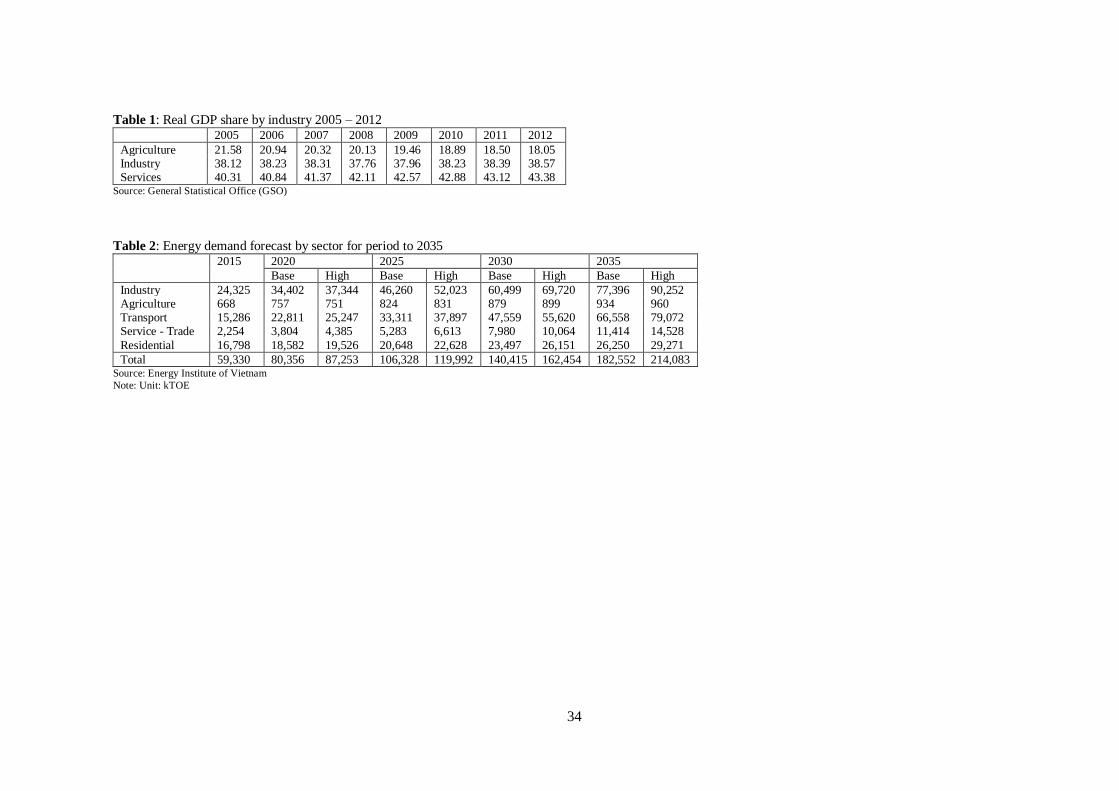
which the industrial contribution in GDP has increased over the last two decades. In fact,

according to the General Statistics Office, the share of the industry and construction to

GDP is 38.6 percent, while that of the agriculture is 18.5 percent in 2012 (see Table 1).

However, many economists and policymakers share some concerns about the country’s

industrialization and its industrial policies. Tran and Doan (2010) discuss the role of

industrialization in reforming economic and employment structure in Vietnam and

suggest that the reforms has failed to shift redundant workers away from agricultural

sector since most of the country’s investment has been allocated to capital-intensive

industries. Nguyen (2011) also examines industrial policy and performance of the

industrial sector and observes that the State-led policy has not yet succeeded in

achieving industrialization due partly to the encouragement of rent-seeking activities,

the failure of creation of new comparative advantages, and poor quality of policy

formulation. It is widely acknowledged that under on-going ASEAN economic

9

integration, Vietnam should adopt an efficient industrialization strategy, where the

industrial sector is a driving force for economic growth.

Recently, access to basic infrastructure particularly in major cities has improved

substantially through significant government’s efforts with official development

assistance (ODA) from developed countries. Currently, electricity is accessible to

almost all households, and clean water and modern sanitation are available to more than

75 percent of all households. In addition, other types of infrastructure, such as the sewer

system and the transportation system, has also received attention especially in urban

areas. Transport infrastructure, including roads and bridges, has been improved with the

expansion of its capacity, but traffic congestion associated with rapid increases in car

and motorbikes and the deterioration of roads caused by disordered urban planning is

still a major social problem in most urban areas. Many infrastructure projects have been

implemented to improve the living standard in urban and rural areas through funds from

ODA, although there still remain many infrastructure-related problems to be solved.

Like other developing and emerging countries, urbanization along with

industrialization has prevailed with the rapid increase in scale in Vietnam. The number

of urban areas in the country has increased significantly from 480 in 1986 to 729 and

755 in 2007 and 2012, respectively (World Bank, 2011). At the same time, urban

population has also increased considerably. In 2000, total urban population in the

country was 18.7 million, accounting for 24 percent of the national population. In 2012,

this number has reached 28.4 million, accounting for 32 percent of the national

population (see Figure 2). In particular, Hanoi and Ho Chi Minh have achieved thee

most rapid urban expansion in Vietnam. According to General Statistics Office (2014)

and Ministry of Construction (2013), the significant increase in urban population has

10

stemmed mainly from the natural increase in urban areas, the migration from rural areas

to urban areas, and the boundary expansion of urban areas. Such massive urbanization

has made the available infrastructure system overloaded, leading to serious social

problems, including energy distribution, environmental pollution, traffic congestion,

and food security.

Vietnam is a resource abundant country with large reserves of primary energy

resources, such as coal, oil, and natural gas, and with a high potential for renewable

energy resources, such as hydropower, biomass, solar, and wind (see, e.g., Toan, Bao,

and Dieu, 2011). In 2012, the total national primary energy supply was around 58.0

million tons of oil equivalent (Mtoe), and the shares of coal, crude oil and petroleum,

gas, and hydropower generation to the total national primary energy were 26%, 27%,

14%, and 8%, respectively (Asian Development Bank, 2016). Concerning the demand

side, the country is more energy intensive compared to those in other Southeast Asian

countries (see, e.g., Do and Sharma, 2011; Toan, Bao, and Dieu, 2011; Nguyen, 2011;

Tang, Tan, and Ozturk, 2016). In 2012, the total final energy consumption in the

country was 49.3 Mtoe, and the shares of residential, transport, service, industrial, and

agriculture uses were 33%, 24%, 3%, 39%, and 1% (Asian Development Bank, 2016).

Do and Sharma (2011) mention that the total energy consumption in Vietnam is

expected to increase to 146 Mtoe in 2025 due to the steady domestic development. The

Energy Institute of Vietnam also reports that the estimated energy demand in 2035 is

within a range between 182 and 214 Mtoe (see Table 2).

Since the supply has dominated the demand, the country has been a net energy

exporter. Net energy exports increased from 0.2 Mtoe in 1990 to 22.0 Mtoe in 2006 and

then declined due to increased domestic demand. In 2012, the country exported 18.0

11

Mtoe of energy, of which 9.4 Mtoe and 8.6 Myoe were crude oil and coal, respectively

(Asian Development Bank, 2016). However, the rapid economic growth is expected to

enforce the country to shift from a net energy exporter to a net energy importer in the

future, which would give rise to energy security problems. Toan, Bao, and Dieu (2011)

project that the country will experience a net deficit of over 28 Mtoe in 2020 and over

104 Mtoe in 2030, even assuming an increase in domestic production of oil, gas, and

coal and the development of other energy resources, such as renewable energy and

nuclear power, under government initiatives of energy policies. Their study also expects

that renewable energy accounts for less than 10 percent of total energy in 2030 with a

decreasing proportion from over 40 percent in 2005, as the country’s economy

develops.

Massive urbanization, along with industrialization, brings about various social

problems, one of which is environmental pollution. Air pollution may be the most

serious issue of environmental pollution, which often causes a lot of damage to human

being and the atmosphere. It is typically caused by the injurious smoke emitted by

automobiles, trains, factories, and other human activities. Examples include pollution

gases, such as sulfur dioxide (SO2), carbon monoxide (CO), carbon dioxide (CO2), and

nitrogen dioxide (NO2), dust pollution, and even smoke from burning leaves and

cigarettes. Vietnam’s remarkable performance of its economic development with

urbanization and industrialization has caused intense pressure on environmental issues.

The quality of the environment in the country has steadily been deteriorated compared

to other countries. The Environmental Performance Index (EPI) presents that the

country is ranked 131th among 180 countries in the 2016 EPI ranking report. In

12

particular, the country shows worse performance for air quality with negative effects on

human health, water, and environmental burden of disease.

The National Environmental Report, published in 2013 by the Ministry of

Natural Resources and Environment (MoNRE), assesses natural and human-made

effects on air quality, air contamination, pollution management, and air protection

measures. This report also illustrates that the country’s economy has generated air

pollution at the high level, e.g., nearly 667,000 tons of SO2, 618,000 tons of NO2, and

6.8 million tons of CO2 annually. According to the University of Natural Resources

and the Environment, 3-4 percent of the entire population currently suffers from

respiratory problems caused by air pollution, and the fraction of people facing

difficulties in breathing is 4-5 times higher in rapidly-growing urban cities with the high

level of air pollution, including dusts, particles, and gases, such as Hanoi, Ho Chi Minh,

and Haiphong than in rural areas.

3 Empirical analysis

This section discusses how urbanization relates to energy use and CO2 emission in

Vietnam by conducting empirical analysis with the province-level panel data covering

63 provinces during the period from 2010 to 2013.

3.1 Methodology and data

To empirically examine the effects of urbanization on energy use and CO2 emission,

this study follows the conventional method in the literature, such as Jones (1991) and

Sadorsky (2013). Specifically, we estimate the following energy and emission

intensities equations:

13

ENEit = α0 + α1URBit + α2URBit × INCit + α3INCit + ∑ ηkxkitk + ϵit,

CO2it = β0 + β1URBit + β2URBit × INCit + β3INCit + ∑ γkxkitk + εit,

where ENEit is energy intensity at province i in year t, CO2it is (CO2) emission

intensity, URBit is the degree of urbanization, INCit is the income level, xkit’s are

other control variables that are expected to affect energy and emission intensities, and

ϵit and εit are the error terms with standard properties. Energy and emission intensities

(ENE and CO2) in each province are calculated by the logs of the total energy

consumption (toe) and the total CO2 emission (ton) divided by provincial real GDP

(thousand USD), respectively. The degree of urbanization (URB), which is our main

explanatory variable, is measured by the log of the percentage of population living in

urban areas. In addition, the income level (INC) is measured by the log of real GDP per

capita (USD) at the province level, which generally reflects the development stage in

the province. Table 3 presents the definitions of variables used in the empirical analysis.

Our main focus is on how the relationship between urbanization and energy

and emission intensities is related to the development stage, which differs substantially

across provinces in Vietnam, like other developing economies facing regional disparity

and inequality. To capture this issue, we include the interaction term of urbanization and

the income level (URB × INC) in the model, which allows us to examine the

dependency of the effect of the urbanization on the income level. More specifically,

differentiating the energy and emission equations with respect to URB yields:

∂ENE

∂URB= α1 + α2INC,

∂CO2

∂URB= β1 + β2INC,

14

where the estimated coefficients on the income level, α2 and β2, determine the

direction of the impact of the income level on the urbanization effect on energy and

emission intensities, respectively. Several contrasting arguments have existed on the

effects of urbanization on energy use and emission, i.e., intensified concentration of

production and consumption brings about the positive and negative linkages of

urbanization with energy use and emission. Given the argument that the development

stage, reflected by the income level, determines the balance of the positive and negative

effects, Poumanyvong and Kaneko (2010) evaluate the urbanization effect in relation to

the income level by using panel data at the national level. Differently from the previous

studies, we examine how urbanization’s role changes over the different stages of

economic development within Vietnam by using panel data at the province level.

Concerning other control variables, we include the log of the industrialization

measure (IND), which is calculated by the industry value added as a percent of GDP,

following the past empirical studies, such as Sadorsky (2013), on the effect of

industrialization. This measure represents manufacturing specialization in each province

(Blanchard, 1992). In addition, this study also includes the measure of foreign direct

investment inflow (FDI) at the province level into our empirical models. The measure of

foreign direct investment inflow (FDI), which is calculated by the log of one plus

foreign direct investment divided by GDP, captures the spillover effects of production

transfer and technology, including the introduction of green technology, from developed

countries (see, e.g., Shahbaz, Nasreen, Abbas, and Anis, 2015). Moreover, the models

take into account the labor market condition (UNE) and human capital (HUM) at the

province level, which are measured by the logs of unemployment rate and the ratio of

people that have high school education and higher, respectively. Furthermore, we also

15

include country and year dummies to control for the country- and year-specific effects

associated with various factors, such as geographic location, resource endowment, and

energy prices. Wooldridge (2015) suggests that the inclusion of such dummies could

mitigate heterogeneity bias and problems with possible spurious regression.

The province-level data of energy consumption and CO2 emission are

collected from the Energy Institute of Vietnam and the Ministry of Natural Resources

and Environment, respectively. The other province-level data used in our empirical

analysis is obtained from Local Statistical Yearbook (2010-2013). This study evaluates

the urbanization effects on energy and emission intensities in relation to the income

level for the whole economy and each of the three sector groups (industrial, agriculture,

and service sectors) by applying three estimation methods: fixed effects (FE),

Prais-Winsten (PW), and first-difference (FD) models. In the estimation for each sector,

we use as the dependent variables the provincial levels of energy and emission

intensities, which are calculated by the logs of the energy consumption (toe) and the

CO2 emission (ton) for each sector divided by the sector’s value added (thousand USD),

respectively. Table 4 presents the summary of statistics for variables used in our

empirical analysis. Tables 5 and 6 show the correlation matrix of variables in the energy

and emission intensities equations. It appears that the urbanization measure (URB) is

generally less correlated with energy and emission intensities for the whole economy

and each of the three sectors. For the whole economy, the correlation between ENE

and URB is 0.111, and that between CO2 and URB is 0.130.

Tables 7, 9, 10, and 11 report the estimated results of the energy intensity

equation for the whole economy and each of the three sectors. Tables 8, 12, 13, and 14

present the estimated results of the emission intensity equation. Following the procedure

16

in the work of Poumanyvong and Kaneko (2010) on the urbanization effects, we first

apply the FE estimation, since our sample may face the heterogeneity problem so that

the OLS estimation could suffer from heterogeneity bias with a common constant term.

The Wooldridge tests for autocorrelation in panel data (Wooldridge, 2002) suggest that

our FE estimation could suffer from serial correlation. In addition, the modified Wald

statistic for groupwise heteroskedasticity in the residuals of a fixed effects model

(Greene, 2000) observes the presence of heteroscedasticity in our FE estimation. These

results imply that the estimated results of the FE estimation could suffer from the biased

problem. Thus, we conduct the PW estimation with panel-corrected standard errors to

control for serial correlation of type AR(1), heteroskedascity, and cross-panel

correlation.

In addition, we also verify our empirical results by applying the first-difference

(FD) estimation, which could mitigate serial correlation problems (Wooldridge, 2015).

In this estimation, we conduct the Wooldridge autocorrelation test (Wooldridge, 2002)

and the Breusch-Pagan heteroskedasticity test (Breusch and Pagan, 1979) for each

model. Once autocorrelation is identified, we apply the Newey-West corrected standard

errors (Newey and West, 1987). If autocorrelation is not identified, and if the

heteroscedasticity is identified, we apply the heteroscedasticity-consistent standard

errors, as recommended by MacKinnon and White (1985). Moreover, we further apply

the seemingly unrelated correlation regression (SUR) model for the robustness check,

since the two error terms of the energy and emission intensities equations might be

correlated each other. Table 15 shows the estimated results of the SUR estimation of the

energy and emission intensities equations.

17

3.2 Results

This subsection presents the estimated results and their implications on how

urbanization is associated with energy and emission intensities in relation to the income

level or development stage for the whole economy and each of the three sectors

(industrial, agriculture, and service sectors) in Vietnam.

3.2.1 The whole economy in Vietnam

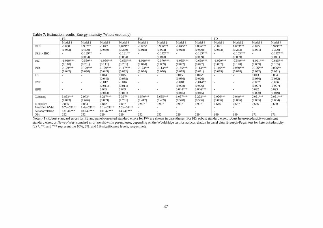
Tables 7 and 8 present that without the interaction term of the urbanization measure and

the income level, URB × INC, the coefficients on URB are negative in both the energy

and emission intensities equations, particularly for the PW estimation, although the FE

and FD estimations show the insignificant results. The negative linkage of urbanization

with energy intensity appears to be consistent with the result of Poumanyvong and

Kaneko (2010) and Li and Lin (2015) in that urbanization decreases energy use in the

low-income countries, including Vietnam. On the other hand, the negative linkage of

urbanization with emission intensity is inconsistent with the result of Poumanyvong and

Kaneko (2010) that observes that urbanization increases emissions although with a

smaller magnitude in the low-income countries than the middle-income countries.

However, once the interaction term URB × INC is included in the models, we can get a

clear picture of the role of the income level in determining the urbanization effect on

energy and emission intensities. Irrespective of the model choices, the coefficients on

URB and URB × INC are significantly positive and negative, respectively, in both the

energy and emission intensities equations. This implies that the urbanization effect

depends highly on the income level, so that urbanization is positively associated with

energy and emission intensities in the low-income provinces, while it is negatively

18

associated with these intensities in the high-income provinces. That is, urbanization

increases energy and emission intensities in the low-income provinces, but it decreases

energy and emission intensities in the high-income provinces.

Possible explanation of the non-linear urbanization effects may be related to

the contrasting arguments on the effect of urbanization. The positive association of

urbanization originates mainly from the argument that urbanization promotes economic

activities through intensified concentration of production and consumption, while the

negative linkage comes mainly from the argument that urbanization brings about

increased energy efficiency through economies of scale. In the low-income provinces,

the former effect would dominate the latter, partly since their economic and industrial

structures are still immature in the less development stage with lack of infrastructure,

such as roads and bridges, so that they may not obtain enough benefit from economies

of scale associated with urbanization. On the other hand, the latter effect dominates the

former, as the income level increases with their development stage advanced due to

increased benefit from economies of scale and improved energy efficiency. Various

infrastructure projects, like the introduction of the public transportation system, might

also help improve energy efficiency and mitigate environmental issues in the

high-income regions. A simple calculation using the estimated results in Tables 7 and 8

suggests that the critical income level differentiating the direction of the urbanization

effect is approximately 800~1000 US dollars (e6.7~e6.9). Table 16 presents energy

and emission intensity elasticities of urbanization, which are based on the estimated

results and the income level of each province in 2013. The energy intensity elasticity

ranges between -0.312 and 0.074, and the emission intensity elasticity ranges between

19

-0.141 and 0.015. Our estimated energy elasticity of urbanization is smaller than the

results of developing countries in Sadorsky (2013).

Our empirical results also present that the coefficients on the income level,

INC, are significantly negative for all models. With the consideration of the negative

coefficients on the interaction term, the high-income provinces in the relatively

advanced development stage are associated with the low levels of energy and emission

intensities, and this negative income effect is intensified by advance of urbanization.

The environmental Kuznets curve (EKC) hypothesis, although there are a lot of debates

on its empirical validity, proposes an inverted U-shaped relationship between

environmental degradation and per capita income, i.e., environmental degradation

increases up to a certain level, an then decreases as income per capita increases (see

Dinda, 2004, for a review on the EKC). The results of the negative relationship of the

income level with emission intensity suggest that although per capita income level is

still relatively low as a low-income country, the Vietnam society might already be in a

right-side position of the environmental Kuznets inverted U-curve, where

environmental degradation decreases as per capita income increases. Stern (2004)

among many studies mentions that a particular innovation tends to be adopted in

developing countries with a short lag once the innovation is adopted in developed

countries. Thus, even for developing countries, like Vietnam, advanced green

technology from developed countries could be adopted by domestic and multinational

firms that are located mainly in the relatively high-income and urbanized provinces

within the country.

It is widely acknowledged that the economic development of Vietnam depends

on rapid industrialization since the early 1990s. Many studies, such as Samouilidis and

20

Mitropoulos (1984), Jones (1989, 1991), and Sadorsky (2013), find that

industrialization leads to large energy consumption due mainly to the argument that the

manufacturing industry with the high value added would be more energy intensive,

compared to the traditional agriculture or basic manufacturing industries. Poumanyvong

and Kaneko (2010) also incorporate the share of industrial activity as a measure of

industrialization into the models and present the positive association of industrialization

with energy consumption, particularly for the low- and middle-income countries, as

well as with CO2 emission, although less clear results about the emission models. Our

estimated results in Tables 7 and 8 suggest that the coefficients on the industrialization

measure, IND, are significantly positive, irrespective of the model choices, for the

energy intensity equation, but those on IND are generally less significant for the

emission intensity equation. These coincide with the results for the low-income

countries, including Vietnam, in Poumanyvong and Kaneko (2010).

Concerning other control variables, the results show that the coefficients on

foreign direct investment (FDI) are generally insignificant in both the energy and

emission intensities equations. FDI, which is considered as one of the important sources

for economic development, especially in developing countries, could give rise to

possibly contrasting effects on energy use and pollution emission through several

channels, such as the transfer of production units as well as advanced or green

technology from advanced countries (see, e.g., Lan, Kakinaka, and Huang, 2012).

Mielnik and Goldemberg (2002) find a clear decline in the energy intensity as FDI

increases in developing economies, probably due to the leapfrogging over old-fashioned

traditional technologies by adopting modern technologies associated with FDI. The

insignificant result of FDI implies that the positive and negative effects of FDI on

21

energy and emission intensities would be balanced and cancelled out each other in

Vietnam.

In addition, the estimated results in Tables 7 and 8 present that the coefficients

on unemployment rate (UNE) are generally insignificant, so that the labor market

condition also has no clear effect on energy and emission intensities. Moreover, our

empirical analysis shows somewhat contrasting results about the effect of human capital

(HUM) in that the coefficients on HUM are positive in the energy intensity equation

and negative in the emission intensity equation, although statistically significant only

for the PW estimations. Possible justifications may include that increased energy

intensity associated with improved human capital comes from an increase in the

energy-intensive industry that generally requires skilled labor with highly-qualified

education, while decreased emission intensity associated with improved human capital

is due to the high incentive to adopt environmental-friendly technology which is often

preferred by the public consisting of well-educated people.

3.2.2 Sector analysis

The previous subsection has discussed how urbanization is associated with energy and

emission intensities in relation to the income level for the whole economy of Vietnam.

In this subsection, we analyze the same issue for each of the three sectors, i.e., the

industrial, agriculture, and service sectors. The model estimation follows the same

procedure as in the previous subsection. Tables 9, 10, and 11 present the estimated

results of the energy intensity equation for the industrial, agriculture, and service sectors.

Similarly, Tables 12, 13, and 14 report the estimated results of the emission intensity

22

equation for the industrial, agriculture, and service sectors. The estimated results are

described as follows.

First, the results concerning the role of urbanization show that the urbanization

effect on energy and emission intensities generally depends on the income level for the

industrial and service sectors. Urbanization would increase energy and emission

intensities in the low-income provinces, while it would decrease these intensities in the

high-income provinces. The threshold income levels differentiating the direction of the

urbanization effect on energy and emission intensities are estimated at around e6.5 =

660 US dollars in the industrial sector and at around e7.0 = 1100 US dollars in the

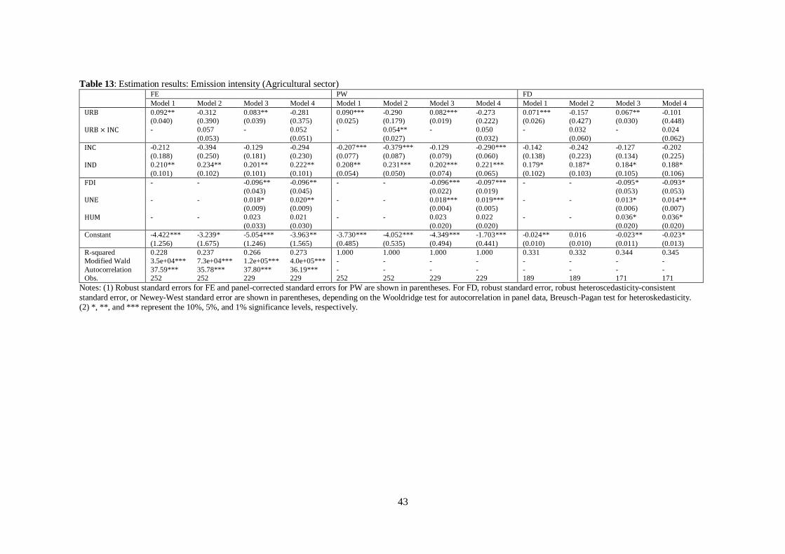
service sector. On the other hand, for the agricultural sector, the urbanization effect on

energy intensity relies on the income level, while that on emission intensity is

independent of the income level. Energy intensity in the agriculture sector would be

increased and decreased as urbanization prevails in the low-income and high-income

provinces, respectively. However, the urbanization effect on emission intensity in the

agriculture sector is insensitive to the income level, although the effect seems to be

positive.

The threshold income level differentiating the direction of the urbanization

effect on energy intensity in the agriculture sector is estimated at around e7.6 = 2000

US dollars. Table 16 presents energy and emission intensity elasticities of urbanization,

which are based on the estimated results and the income level of each province in 2013,

for each sector. The energy intensity elasticity ranges between -0.177 and 0.011,

between -0.228 and 0.253, and between -0.711 and 0.318 for the industrial, agriculture,

and service sectors, respectively. The emission intensity elasticity ranges between

-0.132 and 0.007 and between -0.302 and 0.112 for the industrial and service sectors,

23

respectively. The comparison of the threshold income levels among the three sectors

reveals that the industrial sector has the lowest value, and then the service and

agricultural sectors follow in order. This implies that the urbanization effect on energy

intensity in the industrial sector tends to change from a positive region to a negative

region at the early stage of development (i.e., at the relatively low income level), while

the effect in the agricultural sector tends to change to a negative region at the later stage

of development (i.e., at the relatively high income level). This finding could be justified

by the argument that compared to the agricultural sector, urbanization would promote

energy efficiency of production in the industrial sector, mainly manufacturing, at the

earlier stage of development, since a new industrial technology innovated in developed

countries is easily introduced in the industrial sector of developing countries (Stern,

2004).

Second, concerning the income effects, our empirical analysis generally

presents the clear difference between the agriculture sector and other two sectors. For

the industrial sector, the coefficients on INC and URB × INC are significantly

negative for all estimations. For the service sector, the coefficients on URB × INC are

significantly negative in the energy intensity equations for all estimations, and those on

INC and URB × INC are significantly negative in the emission intensity equations for

the PW estimation. These suggest that for the industrial and service sectors, energy and

emission intensities would decrease with a rise in the income level, and in addition such

a negative income effect is intensified as urbanization prevails. In contrast, for the

agriculture sector, the coefficients on INC and URB × INC are significantly positive

and negative, respectively, in the energy intensity equation for PW and FD estimations.

Given the threshold urbanization level which is estimated at around 2.7~3.0, the

24

income effect on energy intensity is positive in less-urbanized provinces, while it is

negative in highly-urbanized provinces. In the emission intensity equation for the

agriculture sector, the coefficients on INC are significantly negative, although less

clear, and those on URB × INC are insignificant. Thus, an increase in the income level

would decrease emission intensity, independently of the urbanization level.

Third, the empirical analysis by sector also shows the clear sector difference in

the effect of industrialization on energy and emission intensities. The results show that

industrialization decreases energy and emission intensities in the industrial sector. In

general, industrialization tends to increase energy intensity due to the fact that the

industrial sector produces the high value added products, which would be more energy

intensive (Jones, 1989, 1991). However, as industrialization prevails with increased

concentration in the industrial activities, the energy efficiency in the industrial sector

can be improved due to the enhanced benefit from scale economies. The negative effect

of industrialization in the industrial sector confirms that the latter effect dominates the

former. In contrast, the results also present that industrialization increases energy and

emission intensities in the agriculture and service sectors. An industrialized economy

might also promote economic activities in other sectors as the spillover effect, which

could result in the increase in energy use in other sectors.

Finally, concerning other controls, the estimated results related to FDI effects

suggest that FDI inflows decrease energy and emission intensities in the agriculture

sector. On the other hand, FDI inflows increase energy intensity in the industrial sector

and emission intensity in the service sector, although the corresponding estimated

coefficients are significant only for the PW estimation. In addition, the analysis also

presents that unemployment rates reflecting the labor market condition are positively

25

associated with energy and emission intensities in the agriculture sector. At the same

time, the results show that provinces with the high unemployment rate tend to face the

low level of energy intensity in the industrial sector. Furthermore, our analysis observes

that although some estimated results are less clear, provinces with high human capital

are likely to incur high energy intensity in the industrial and agriculture sectors and high

emission intensity in the agriculture sector but to achieve low emission intensity in the

service sector.

4 Conclusion

The study has analyzed how urbanization is associated with energy and CO2 emission

intensities in relation to the income level, which reflects the development stage, by

using the province-level panel data of Vietnam. The empirical analysis has been

conducted not only for the whole country, but also for the three main sectors of the

Vietnamese economy: the industrial, agriculture, and service sectors. This study is the

first attempt which conducts empirical analysis on the urbanization effect on energy use

and emissions in newly emerging countries, like Vietnam, with the full set of three main

economic sectors at the province-level. In addition, this study has also examined the

roles of other important factors, such as industrialization.

The main results have shown the negative effects of urbanization on energy and

emission intensities with the relatively small magnitude for the whole economy in

Vietnam. However, once we introduce the role of the income level in determining the

urbanization effect, the results have shown a clear picture that such an urbanization

effect depends highly on the income level in each province. Urbanization is positively

associated with energy and emission intensities in low-income provinces, while it is

26

negatively associated with energy and emission intensities in high-income provinces.

The analysis by sector has also presented the clear evidence supportive of the

heterogeneous effects on energy and emission intensities in relation to the income level.

In general, most developing countries suffer from reginal income inequality,

which is one of the most important agenda for sustainable economic development. The

existence of regional income inequality would enable our empirical findings to help

understand the regional differences in the role of urbanization in identifying energy and

environmental issues in Vietnam and other emerging countries. In addition, our results

in this study contribute not only to the literature but also to encourage policymakers and

urban planners to pay attention to the urbanization effect on energy and environmental

issues for appropriate policy planning to promote sustainable economic development

with environmental protection.

27

References

Asian Development Bank (2016). Viet Nam: Energy sector assessment, strategy, and

road map. Asian Development Bank, Mandaluyong City, Philippines.

Blanchard, O., 1992. Energy consumption and modes of industrialization: Four

developing countries. Energy Policy 20, 1174-1185.

Breusch, T.S., Pagan, A.R., 1979. A simple test for heteroscedasticity and random

coefficient variation. Econometrica 47, 1287-1294.

Cole, M.A., Neumayer, E., 2004. Examining the impact of demographic factors on air

pollution. Population and Environment 26, 5-21.

Dinda, S., 2004. Environmental Kuznets curve hypothesis: A survey. Ecological

Economics 49, 431-455.

Do, T.M., Sharma, D., 2011. Vietnam’s energy sector: A review of current energy

policies and strategies. Energy Policy 39, 5770-5777.

General Statistics Office. (2014). Statistical year book 2014. Statistics Publishing House,

Hanoi, Vietnam.

Greene, W.H., 2000. Econometric Analysis, Fourth Edition. Prentice Hall, New Jersey.

Holtedahl, P., Joutz, F.L., 2004. Residential electricity demand in Taiwan. Energy


Jones, D.W., 1989. Urbanization and energy use in economic development. Energy

Journal 10, 29-44.

Jones, D.W., 1991. How urbanization affects energy-use in developing countries.

Energy Policy 19, 621-630.

Lan, J., Kakinaka, M., Huang, X., 2011. Foreign direct investment, human capital and

environmental pollution in China. Environmental and Resource Economics 51,

255-275.

Li, K., Lin, B., 2015. Impacts of urbanization and industrialization on energy

consumption/CO2 emissions: Does the level of development matter? Renewable

and Sustainable Energy Reviews 52, 1107-1122.

Liddle, B., 2004. Demographic dynamics and per capita environmental impact: Using

panel regressions and household decompositions to examine population and

transport. Population and Environment 26, 23-39.

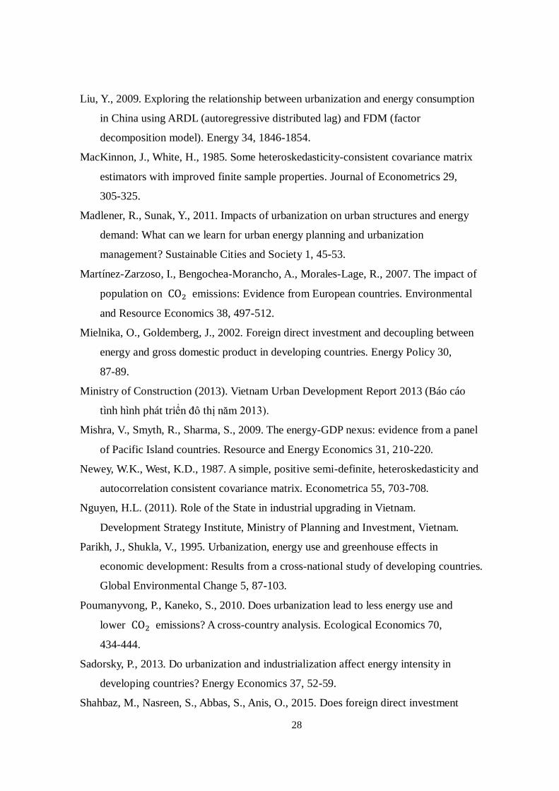
28

Liu, Y., 2009. Exploring the relationship between urbanization and energy consumption

in China using ARDL (autoregressive distributed lag) and FDM (factor

decomposition model). Energy 34, 1846-1854.

MacKinnon, J., White, H., 1985. Some heteroskedasticity-consistent covariance matrix

estimators with improved finite sample properties. Journal of Econometrics 29,

305-325.

Madlener, R., Sunak, Y., 2011. Impacts of urbanization on urban structures and energy

demand: What can we learn for urban energy planning and urbanization

management? Sustainable Cities and Society 1, 45-53.

Martínez-Zarzoso, I., Bengochea-Morancho, A., Morales-Lage, R., 2007. The impact of

population on CO2 emissions: Evidence from European countries. Environmental

and Resource Economics 38, 497-512.

Mielnika, O., Goldemberg, J., 2002. Foreign direct investment and decoupling between

energy and gross domestic product in developing countries. Energy Policy 30,

87-89.

Ministry of Construction (2013). Vietnam Urban Development Report 2013 (Báo cáo

tình hình phát triển đô thị năm 2013).

Mishra, V., Smyth, R., Sharma, S., 2009. The energy-GDP nexus: evidence from a panel

of Pacific Island countries. Resource and Energy Economics 31, 210-220.

Newey, W.K., West, K.D., 1987. A simple, positive semi-definite, heteroskedasticity and

autocorrelation consistent covariance matrix. Econometrica 55, 703-708.

Nguyen, H.L. (2011). Role of the State in industrial upgrading in Vietnam.

Development Strategy Institute, Ministry of Planning and Investment, Vietnam.

Parikh, J., Shukla, V., 1995. Urbanization, energy use and greenhouse effects in

economic development: Results from a cross-national study of developing countries.

Global Environmental Change 5, 87-103.

Poumanyvong, P., Kaneko, S., 2010. Does urbanization lead to less energy use and

lower CO2 emissions? A cross-country analysis. Ecological Economics 70,

434-444.

Sadorsky, P., 2013. Do urbanization and industrialization affect energy intensity in

developing countries? Energy Economics 37, 52-59.

Shahbaz, M., Nasreen, S., Abbas, S., Anis, O., 2015. Does foreign direct investment

29

impede environmental quality in high-, middle-, and low-income countries? Energy


Samouilidis, J.E., Mitropoulos, C.S., 1984. Energy and economic growth in

industrialized countries: The case of Greece. Energy Economics 6, 191-201.

Stern, D.I., 2004. The rise and fall of the environmental Kuznets curve. World

Development 32, 1419-1439.

Tang, C.F., Tan, B.W., Ozturk, I., 2016. Energy consumption and economic growth in

Vietnam. Renewable and Sustainable Energy Reviews 54, 1506-1514.

Toan, P.K., Bao, N.M., Dieu, N.H., 2011. Energy supply, demand, and policy in Viet

Nam, with future projections. Energy Policy 39, 6814-6826.

Wooldridge, J.M., 2002. Econometric Analysis of Cross Section and Panel Data. MIT

Press, Cambridge, MA.

Wooldridge, J.M., 2015. Introductory Econometrics: A Modern Approach, Sixth Edition.

South-Western Pub.

World Bank. (2011). Vietnam Urbanization Review: Technical Assistance Report. World

Bank.

York, R., 2007. Demographic trends and energy consumption in European Union

Nations, 1960-2025. Social Science Research 36, 855-872.

York, R., Rosa, E.A., Dietz, T., 2003. STIRPAT, IPAT and ImPACT: Analytical tools for

unpacking the driving forces of environmental impacts. Ecological Economics 46,

351-365.

Zhang, C., Lin, Y., 2012. Panel estimation for urbanization, energy consumption and

CO2 emissions: A regional analysis in China. Energy Policy 49, 488-498.

30

Figure 1: Fraction of urban population

Source: General Statistical Office (GSO)

Figure 2: Comparison of per capita GDP (in log scale)

Source: World Bank Indicator

31

Figure 3: Energy intensity

Notes: Energy intensity is calculated by energy consumption (toe) divided by gross domestic product (thousand VND).

Figure 4: Emission intensity

Notes: Emission intensity is calculated by emission gas (ton) divided by gross domestic product (million VND).

32

Figure 5: Energy intensity

Notes: Average over the sample period. Energy intensity is calculated by energy consumption (toe) divided by gross domestic product (thousand VND).

33

Figure 6: Emission intensity

Notes: Average over the sample period. Emission intensity is calculated by emission gas (ton) divided by gross domestic product (million VND).

34

Table 1: Real GDP share by industry 2005 – 2012 2005 2006 2007 2008 2009 2010 2011 2012

Agriculture 21.58 20.94 20.32 20.13 19.46 18.89 18.50 18.05 Industry 38.12 38.23 38.31 37.76 37.96 38.23 38.39 38.57 Services 40.31 40.84 41.37 42.11 42.57 42.88 43.12 43.38

Source: General Statistical Office (GSO)

Table 2: Energy demand forecast by sector for period to 2035 2015 2020 2025 2030 2035

Base High Base High Base High Base High

Industry 24,325 34,402 37,344 46,260 52,023 60,499 69,720 77,396 90,252 Agriculture 668 757 751 824 831 879 899 934 960 Transport 15,286 22,811 25,247 33,311 37,897 47,559 55,620 66,558 79,072 Service - Trade 2,254 3,804 4,385 5,283 6,613 7,980 10,064 11,414 14,528

Residential 16,798 18,582 19,526 20,648 22,628 23,497 26,151 26,250 29,271

Total 59,330 80,356 87,253 106,328 119,992 140,415 162,454 182,552 214,083 Source: Energy Institute of Vietnam

Note: Unit: kTOE

35

Table 3: Description of the variables in the period 2010 – 2013 Variable Name of variable Definition Data source

ENE Energy intensity Energy consumption divided by real GDP

Energy Institute of Vietnam

CO2 CO2 emission intensity

CO2 emission divided by real GDP Ministry of Natural Resources and Environment

INC Income level Real GDP per capita Local statistical yearbook (2010

- 2013)

IND Industrialization The ratio of the industry's value added to GDP

Local statistical yearbook (2010 - 2013)

URB Urbanization The ratio of the population living in urban areas


FDI FDI One plus FDI at constant price 2010 divided by real GDP


UNE Unemployment rate

Unemployment rate Local statistical yearbook (2010 - 2013)

HUM Human capacity The ratio of population who has education of high school or upper


Note: All values are in terms of the logarithm.

Table 4: Summary statistics

Obs Mean Std. Dev. Min Max

ENE

Total 252 -0.786 0.438 -1.954 0.479 Industrial sector 252 -0.009 0.725 -2.324 1.041 Agriculture sector 252 -5.096 2.214 -10.580 -0.199 Service sector 252 -2.347 1.164 -5.838 -0.116

CO2

Total 252 -0.763 1.706 -5.878 2.310

Agriculture sector 252 0.150 1.582 -4.837 3.036 Industrial sector 252 -4.887 2.086 -10.537 -1.176 Service sector 252 -4.934 3.038 -10.661 2.786

INC 252 6.931 0.504 5.870 9.076 URB 252 3.133 0.531 2.267 4.469 IND 252 3.516 0.406 2.447 4.461

FDI 229 0.051 0.089 0.000 0.879

UNE 229 0.497 0.646 -1.470 1.900 HUM 229 1.491 0.443 0.708 3.122

Note: All values are in terms of the logarithm.

36

Table 5: Correlation matrix (energy intensities) ENE ENEI ENEA ENES INC URB IND

ENE 1.000

ENEI 0.571 1.000

ENEA 0.055 -0.183 1.000

ENES 0.020 -0.256 0.276 1.000

INC 0.061 0.007 0.225 -0.215 1.000

URB 0.111 -0.021 0.155 -0.011 0.574 1.000

IND 0.430 -0.163 0.070 -0.187 0.407 0.211 1.000

Notes: ENEI, ENEA, and ENES represent energy intensity (ENE) in the industrial, agriculture, and

service sectors, respectively.

Table 6: Correlation matrix (emission intensities)

CO2 CO2I CO2A CO2S INC URB IND

CO2 1.000

CO2I 0.945 1.000

CO2A 0.371 0.280 1.000

CO2S 0.370 0.199 -0.011 1.000

INC 0.038 -0.118 0.177 0.272 1.000 URB 0.130 0.085 0.172 0.220 0.574 1.000

IND 0.428 0.211 0.402 0.141 0.407 0.211 1.000

Notes: CO2I, CO2A, and CO2S represent emission intensity (CO2) in the industrial, agriculture, and

service sectors, respectively.

37

Table 7: Estimation results: Energy intensity (Whole economy) FE PW FD

Model 1 Model 2 Model 3 Model 4 Model 1 Model 2 Model 3 Model 4 Model 1 Model 2 Model 3 Model 4

URB -0.038 0.937** -0.047 0.879** -0.035* 0.966*** -0.045** 0.896*** -0.021 1.053*** -0.025 0.979***

(0.042) (0.400) (0.039) (0.399) (0.018) (0.094) (0.018) (0.070) (0.063) (0.283) (0.031) (0.300)

URB × INC - -0.139** - -0.131** - -0.142*** - -0.133*** - -0.153*** - -0.142***

(0.054) (0.054) (0.013) (0.009) (0.039) (0.041)

INC -1.019*** -0.580** -1.086*** -0.665*** -1.019*** -0.570*** -1.085*** -0.658*** -1.020*** -0.549*** -1.061*** -0.615***

(0.110) (0.231) (0.111) (0.231) (0.044) (0.059) (0.072) (0.077) (0.067) (0.148) (0.059) (0.155)

IND 0.179*** 0.120*** 0.170*** 0.117*** 0.173*** 0.113*** 0.165*** 0.113*** 0.116*** 0.080*** 0.106*** 0.076**

(0.042) (0.030) (0.045) (0.032) (0.024) (0.020) (0.029) (0.021) (0.029) (0.028) (0.032) (0.031)

FDI - - 0.044 0.045 - - 0.045 0.046* - - 0.043 0.034

(0.045) (0.038) (0.036) (0.026) (0.036) (0.032)

UNE - - -0.012 -0.016 - - -0.010 -0.014** - - -0.002 -0.006

(0.011) (0.011) (0.008) (0.006) (0.007) (0.007)

HUM - - 0.045 0.049 - - 0.044*** 0.046*** - - 0.022 0.023

(0.043) (0.041) (0.015) (0.015) (0.020) (0.019)

Constant 5.833*** 2.973* 6.217*** 3.367* 6.570*** 5.635*** 6.037*** 3.222*** 0.026*** 0.049*** 0.031*** 0.031***

(0.873) (1.676) (0.889) (1.701) (0.412) (0.439) (0.548) (0.506) (0.006) (0.006) (0.005) (0.004)

R-squared 0.836 0.853 0.842 0.857 0.997 0.997 0.997 0.997 0.646 0.687 0.656 0.690

Modified Wald 6.7e+05*** 1.4e+05*** 3.1e+05*** 5.2e+04*** - - - - - - - -

Autocorrelation 131.46*** 183.40*** 101.47*** 143.40*** - - - - - - - -

Obs. 252 252 229 229 252 252 229 229 189 189 171 171

Notes: (1) Robust standard errors for FE and panel-corrected standard errors for PW are shown in parentheses. For FD, robust standard error, robust heteroscedasticity-consistent

standard error, or Newey-West standard error are shown in parentheses, depending on the Wooldridge test for autocorrelation in panel data, Breusch-Pagan test for heteroskedasticity. (2) *, **, and *** represent the 10%, 5%, and 1% significance levels, respectively.

38

Table 8: Estimation results: Emission intensity (Whole economy) FE PW FD


URB -0.023 0.420*** -0.029 0.356** -0.024*** 0.410*** -0.029*** 0.349*** -0.025 0.357*** -0.027 0.308***

(0.030) (0.150) (0.029) (0.153) (0.009) (0.051) (0.009) (0.066) (0.018) (0.110) (0.018) (0.113)

URB × INC - -0.063*** - -0.055** - -0.062*** - -0.054*** - -0.054*** - -0.048***

(0.021) (0.021) (0.007) (0.010) (0.015) (0.016)

INC -1.049*** -0.849*** -1.052*** -0.877*** -1.045*** -0.850*** -1.050*** -0.877*** -1.016*** -0.848*** -1.016*** -0.867***

(0.036) (0.079) (0.039) (0.079) (0.022) (0.027) (0.030) (0.045) (0.023) (0.056) (0.025) (0.058)

IND 0.040** 0.013 0.032 0.010 0.037*** 0.012* 0.030*** 0.009 0.021 0.008 0.015 0.005

(0.019) (0.015) (0.020) (0.017) (0.010) (0.007) (0.011) (0.007) (0.013) (0.013) (0.015) (0.015)

FDI - - 0.001 0.002 - - 0.002 0.002 - - -0.002 -0.005

(0.018) (0.016) (0.012) (0.009) (0.019) (0.018)

UNE - - 0.0002 -0.002 - - 0.000 -0.001 - - 0.000 -0.001

(0.004) (0.004) (0.002) (0.002) (0.003) (0.002)

HUM - - -0.011 -0.009 - - -0.010** -0.009** - - -0.006 -0.005

(0.014) (0.015) (0.005) (0.003) (0.007) (0.007)

Constant 6.512*** 5.210*** 6.459*** 5.225*** 8.703*** 8.925*** 9.305*** 9.151*** 0.043*** 0.037*** 0.043*** 0.043***

(0.304) (0.560) (0.324) (0.570) (0.178) (0.202) (0.204) (0.321) (0.003) (0.003) (0.002) (0.003)

R-squared 0.962 0.966 0.964 0.967 1.000 1.000 1.000 1.000 0.904 0.910 0.905 0.910



Obs. 252 252 229 229 252 252 229 229 189 189 171 171



39

Table 9: Estimation results: Energy intensity (Industrial sector) FE PW FD


URB -0.039 0.478** -0.048 0.409** -0.039** 0.486*** -0.048*** 0.413*** -0.025 0.531*** -0.029 0.463***

(0.032) (0.207) (0.029) (0.197) (0.016) (0.037) (0.018) (0.039) (0.023) (0.155) (0.045) (0.166)

URB × INC - -0.074** - -0.065** - -0.074*** - -0.065*** - -0.079*** - -0.070**

(0.029) (0.028) (0.004) (0.004) (0.022) (0.024)

INC -1.059*** -0.826*** -1.102*** -0.894*** -1.058*** -0.823*** -1.102*** -0.892*** -1.053*** -0.809*** -1.076*** -0.857***

(0.060) (0.112) (0.058) (0.106) (0.026) (0.027) (0.043) (0.044) (0.037) (0.080) (0.040) (0.085)

IND -0.931*** -0.962*** -0.943*** -0.969*** -0.931*** -0.964*** -0.943*** -0.970*** -0.959*** -0.978*** -0.970*** -0.985***

(0.023) (0.021) (0.023) (0.022) (0.011) (0.009) (0.013) (0.009) (0.019) (0.022) (0.022) (0.024)

FDI - - 0.035 0.035 - - 0.035* 0.036** - - 0.030 0.026

(0.028) (0.025) (0.019) (0.015) (0.024) (0.021)

UNE - - -0.007 -0.009 - - -0.007* -0.009*** - - -0.002 -0.004

(0.006) (0.006) (0.004) (0.003) (0.005) (0.004)

HUM - - 0.014 0.016 - - 0.014* 0.016** - - 0.005 0.006

(0.018) (0.017) (0.008) (0.007) (0.010) (0.009)

Constant 10.787*** 9.268*** 11.043*** 9.602*** 10.794*** 9.254*** 12.171*** 12.918*** 0.024*** 0.043*** 0.027*** 0.027***

(0.490) (0.806) (0.470) (0.756) (0.231) (0.198) (0.387) (0.400) (0.003) (0.005) (0.004) (0.003)

R-squared 0.979 0.981 0.981 0.983 1.000 1.000 1.000 1.000 0.952 0.956 0.954 0.957



Obs. 252 252 229 229 252 252 229 229 189 189 171 171



40

Table 10: Estimation results: Energy intensity (Agricultural sector) FE PW FD


URB 0.115 1.418* 0.105 1.249* 0.116*** 1.451*** 0.107*** 1.279*** 0.118 1.827*** 0.113 1.724**

(0.071) (0.739) (0.072) (0.715) (0.041) (0.407) (0.023) (0.432) (0.076) (0.645) (0.085) (0.686)

URB × INC - -0.185* - -0.162 - -0.190*** - -0.166*** - -0.243*** - -0.229**

(0.103) (0.100) (0.057) (0.062) (0.089) (0.095)

INC -0.099 0.488 -0.038 0.482 -0.097 0.504*** -0.040 0.492*** -0.058 0.692** -0.098 0.619*

(0.300) (0.403) (0.321) (0.385) (0.098) (0.145) (0.121) (0.123) (0.183) (0.305) (0.208) (0.324)

IND 0.556*** 0.478** 0.563*** 0.499** 0.552*** 0.472*** 0.559*** 0.494*** 0.435*** 0.377** 0.439** 0.391**

(0.180) (0.189) (0.187) (0.194) (0.078) (0.090) (0.078) (0.077) (0.148) (0.159) (0.170) (0.178)

FDI - - -0.188** -0.186** - - -0.188*** -0.186*** - - -0.129 -0.144

(0.090) (0.084) (0.039) (0.043) (0.106) (0.102)

UNE - - 0.017 0.012 - - 0.017*** 0.011* - - 0.015 0.009

(0.027) (0.026) (0.005) (0.007) (0.015) (0.014)

HUM - - 0.107* 0.111* - - 0.106*** 0.110*** - - 0.080** 0.081**

(0.055) (0.057) (0.040) (0.041) (0.036) (0.035)

Constant -6.667*** -10.492*** -7.255*** -10.744*** -8.244*** -12.175*** -7.734*** -12.242*** 0.014 0.056*** 0.022*** 0.022

(2.172) (2.773) (2.266) (2.580) (0.587) (0.852) (0.915) (0.815) (0.015) (0.018) (0.017) (0.022)

R-squared 0.480 0.497 0.495 0.508 0.999 0.999 0.999 0.999 0.180 0.217 0.195 0.226



Obs. 252 252 229 229 252 252 229 229 189 189 171 171



41

Table 11: Estimation results: Energy intensity (Service sector) FE PW FD


URB 0.003 2.613*** 0.014 2.528*** 0.000 2.607*** 0.008 2.512*** 0.027 2.977*** 0.032 2.954***

(0.122) (0.814) (0.128) (0.878) (0.043) (0.253) (0.037) (0.292) (0.190) (0.945) (0.202) (1.030)

URB × INC - -0.371*** - -0.357*** - -0.371*** - -0.355*** - -0.420*** - -0.414***

(0.110) (0.119) (0.033) (0.038) (0.129) (0.141)

INC -1.129*** 0.048 -1.205*** -0.063 -1.119*** 0.050 -1.195*** -0.063 -1.347*** -0.052 -1.373*** -0.073

(0.406) (0.441) (0.443) (0.467) (0.122) (0.189) (0.123) (0.216) (0.459) (0.329) (0.509) (0.375)

IND 0.989*** 0.832*** 1.000*** 0.858*** 0.985*** 0.830*** 0.994*** 0.854*** 1.027*** 0.928*** 1.032*** 0.944***

(0.227) (0.199) (0.234) (0.201) (0.050) (0.078) (0.051) (0.088) (0.293) (0.231) (0.303) (0.238)

FDI - - 0.063 0.068 - - 0.065 0.070 - - 0.045 0.019

(0.119) (0.126) (0.089) (0.086) (0.173) (0.119)

UNE - - 0.004 -0.007 - - 0.006 -0.006 - - -0.004 -0.016

(0.028) (0.025) (0.012) (0.015) (0.019) (0.016)

HUM - - 0.022 0.031 - - 0.030 0.036 - - -0.035 -0.034

(0.058) (0.060) (0.059) (0.068) (0.069) (0.053)

Constant 2.060 -5.602* 2.406 -5.202 0.770 -4.254*** 1.186 -3.572** 0.040 0.083*** 0.043 0.042

(2.725) (3.094) (2.983) (3.240) (0.811) (1.495) (0.870) (1.662) (0.032) (0.030) (0.037) (0.035)

R-squared 0.490 0.542 0.493 0.539 0.998 0.998 0.998 0.998 0.410 0.459 0.420 0.464



Obs. 252 252 229 229 252 252 229 229 189 189 171 171



42

Table 12: Estimation results: Emission intensity (Industrial sector) FE PW FD


URB -0.026 0.390*** -0.032 0.303** -0.025** 0.386*** -0.031*** 0.304*** -0.020 0.365*** -0.023 0.309***

(0.030) (0.147) (0.028) (0.147) (0.011) (0.034) (0.011) (0.044) (0.018) (0.102) (0.018) (0.088)

URB × INC - -0.059*** - -0.048** - -0.058*** - -0.048*** - -0.055*** - -0.047***

(0.021) (0.021) (0.006) (0.007) (0.014) (0.012)

INC -1.061*** -0.874*** -1.070*** -0.917*** -1.056*** -0.871*** -1.064*** -0.911*** -1.029*** -0.860*** -1.033*** -0.885***

(0.035) (0.076) (0.037) (0.074) (0.020) (0.022) (0.026) (0.038) (0.019) (0.049) (0.020) (0.044)

IND -0.962*** -0.987*** -0.971*** -0.990*** -0.965*** -0.988*** -0.973*** -0.991*** -0.979*** -0.992*** -0.984*** -0.994***

(0.017) (0.014) (0.018) (0.016) (0.010) (0.007) (0.011) (0.008) (0.011) (0.011) (0.012) (0.012)

FDI - - -0.000 0.000 - - -0.000 -0.001 - - -0.007 -0.010

(0.017) (0.015) (0.013) (0.011) (0.019) (0.018)

UNE - - 0.002 0.001 - - 0.002 0.000 - - 0.001 -0.001

(0.003) (0.003) (0.002) (0.001) (0.002) (0.002)

HUM - - -0.011 -0.009 - - -0.009 -0.008 - - -0.002 -0.002

(0.013) (0.014) (0.006) (0.005) (0.005) (0.005)

Constant 11.045*** 9.824*** 11.018*** 9.924*** 13.401*** 12.613*** 13.546*** 12.929*** 0.049*** 0.037*** 0.050*** 0.050***

(0.294) (0.539) (0.307) (0.529) (0.164) (0.158) (0.216) (0.269) (0.002) (0.002) (0.002) (0.002)

R-squared 0.988 0.990 0.990 0.991 1.000 1.000 1.000 1.000 0.981 0.983 0.983 0.984



Obs. 252 252 229 229 252 252 229 229 189 189 171 171



43

Table 13: Estimation results: Emission intensity (Agricultural sector) FE PW FD


URB 0.092** -0.312 0.083** -0.281 0.090*** -0.290 0.082*** -0.273 0.071*** -0.157 0.067** -0.101

(0.040) (0.390) (0.039) (0.375) (0.025) (0.179) (0.019) (0.222) (0.026) (0.427) (0.030) (0.448)

URB × INC - 0.057 - 0.052 - 0.054** - 0.050 - 0.032 - 0.024

(0.053) (0.051) (0.027) (0.032) (0.060) (0.062)

INC -0.212 -0.394 -0.129 -0.294 -0.207*** -0.379*** -0.129 -0.290*** -0.142 -0.242 -0.127 -0.202

(0.188) (0.250) (0.181) (0.230) (0.077) (0.087) (0.079) (0.060) (0.138) (0.223) (0.134) (0.225)

IND 0.210** 0.234** 0.201** 0.222** 0.208** 0.231*** 0.202*** 0.221*** 0.179* 0.187* 0.184* 0.188*

(0.101) (0.102) (0.101) (0.101) (0.054) (0.050) (0.074) (0.065) (0.102) (0.103) (0.105) (0.106)

FDI - - -0.096** -0.096** - - -0.096*** -0.097*** - - -0.095* -0.093*

(0.043) (0.045) (0.022) (0.019) (0.053) (0.053)

UNE - - 0.018* 0.020** - - 0.018*** 0.019*** - - 0.013* 0.014**

(0.009) (0.009) (0.004) (0.005) (0.006) (0.007)

HUM - - 0.023 0.021 - - 0.023 0.022 - - 0.036* 0.036*

(0.033) (0.030) (0.020) (0.020) (0.020) (0.020)

Constant -4.422*** -3.239* -5.054*** -3.963** -3.730*** -4.052*** -4.349*** -1.703*** -0.024** 0.016 -0.023** -0.023*

(1.256) (1.675) (1.246) (1.565) (0.485) (0.535) (0.494) (0.441) (0.010) (0.010) (0.011) (0.013)

R-squared 0.228 0.237 0.266 0.273 1.000 1.000 1.000 1.000 0.331 0.332 0.344 0.345



Obs. 252 252 229 229 252 252 229 229 189 189 171 171



44

Table 14: Estimation results: Emission intensity (Service sector) FE PW FD


URB -0.020 0.884 -0.009 0.998 -0.020 0.880*** -0.008 0.996*** -0.021 0.993 -0.014 1.129

(0.105) (0.698) (0.106) (0.767) (0.030) (0.150) (0.031) (0.151) (0.063) (0.962) (0.060) (1.041)

URB × INC - -0.129 - -0.143 - -0.128*** - -0.143*** - -0.144 - -0.162

(0.092)

(0.101) (0.021)

(0.020)

(0.131)

(0.142)

INC -1.242*** -0.834*** -1.295*** -0.838** -1.248*** -0.847*** -1.297*** -0.842*** -1.432*** -0.987*** -1.402*** -0.893***

(0.311) (0.309) (0.340) (0.336) (0.123) (0.170) (0.119) (0.185) (0.380) (0.265) (0.395) (0.305)

IND 0.642*** 0.588*** 0.638*** 0.582*** 0.648*** 0.598*** 0.642*** 0.587*** 0.772*** 0.738*** 0.776*** 0.742***

(0.237) (0.211) (0.237) (0.209) (0.063) (0.072) (0.074) (0.088) (0.286) (0.258) (0.292) (0.263)

FDI - - 0.156 0.158 - - 0.155* 0.156* - - 0.079 0.069

(0.106) (0.112)

(0.086) (0.083)

(0.089) (0.086)

UNE - - 0.006 0.001 - - 0.005 0.000 - - -0.006 -0.011

(0.015) (0.014)

(0.011) (0.012)

(0.011) (0.010)

HUM - - -0.062 -0.058 - - -0.063 -0.060 - - -0.080* -0.080*

(0.038) (0.042)

(0.049) (0.052)

(0.043) (0.043)

Constant 1.508 -1.145 1.937 -1.090 1.600*** 6.017*** 9.028*** 8.252*** 0.003 0.043 -0.003 -0.003

(1.892) (2.354) (2.079) (2.529) (0.889) (1.083) (0.816) (1.507) (0.025) (0.026) (0.027) (0.027)

R-squared 0.778 0.782 0.780 0.785 1.000 1.000 1.000 1.000 0.464 0.472 0.469 0.478



Obs. 252 252 229 229 252 252 229 229 189 189 171 171



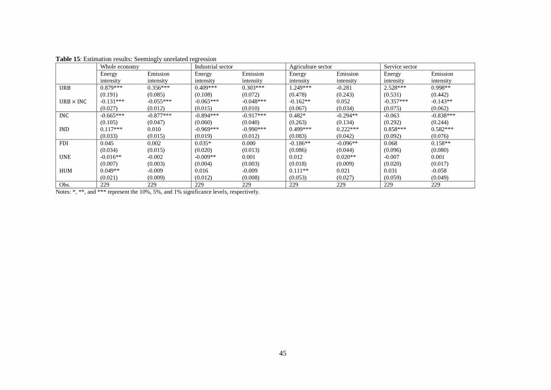
45

Table 15: Estimation results: Seemingly unrelated regression Whole economy Industrial sector Agriculture sector Service sector

Energy intensity

Emission intensity

Energy intensity

Emission intensity

Energy intensity

Emission intensity

Energy intensity

Emission intensity

URB 0.879*** 0.356*** 0.409*** 0.303*** 1.249*** -0.281 2.528*** 0.998**

(0.191) (0.085) (0.108) (0.072) (0.478) (0.243) (0.531) (0.442)

URB × INC -0.131*** -0.055*** -0.065*** -0.048*** -0.162** 0.052 -0.357*** -0.143**

(0.027) (0.012) (0.015) (0.010) (0.067) (0.034) (0.075) (0.062)

INC -0.665*** -0.877*** -0.894*** -0.917*** 0.482* -0.294** -0.063 -0.838*** (0.105) (0.047) (0.060) (0.040) (0.263) (0.134) (0.292) (0.244)

IND 0.117*** 0.010 -0.969*** -0.990*** 0.499*** 0.222*** 0.858*** 0.582*** (0.033) (0.015) (0.019) (0.012) (0.083) (0.042) (0.092) (0.076)

FDI 0.045 0.002 0.035* 0.000 -0.186** -0.096** 0.068 0.158** (0.034) (0.015) (0.020) (0.013) (0.086) (0.044) (0.096) (0.080)

UNE -0.016** -0.002 -0.009** 0.001 0.012 0.020** -0.007 0.001 (0.007) (0.003) (0.004) (0.003) (0.018) (0.009) (0.020) (0.017)

HUM 0.049** -0.009 0.016 -0.009 0.111** 0.021 0.031 -0.058

(0.021) (0.009) (0.012) (0.008) (0.053) (0.027) (0.059) (0.049)

Obs. 229 229 229 229 229 229 229 229

Notes: *, **, and *** represent the 10%, 5%, and 1% significance levels, respectively.

46

Table 16: Energy and emission intensity elasticities of urbanization Average income

province

Highest income

province

Lowest income

province

Energy intensity elasticities

Whole economy -0.042 -0.312 0.074

Industrial -0.045 -0.177 0.011

Agriculture 0.109 -0.228 0.253

Service 0.009 -0.711 0.318

Emission intensity elasticities

Whole economy -0.032 -0.141 0.015

Industrial -0.034 -0.132 0.007

Agriculture 0.082 - -

Service -0.012 -0.302 0.112

Notes: (1) Columns of average income, lowest income, and highest income provinces show

elasticities for provinces with the average, the lowest, and the highest level of provincial GDP

per capita over all provinces in 2013. (2) The calculation is based on the results of Model 4 of

the PW estimation, except that the result of Model 3 of the PW estimation for emission intensity

elasticity in the agriculture sector.

Documents

How does urbanization a ect energy and CO2 emission ... · Social Design Engineering Series SDES-2017-8 How does urbanization a ect energy and CO2 emission intensities in Vietnam?