How Do They Know and What Could We Do? - SOA · How Do They Know and What Could We Do? The Science of 21st Century Climate Projections . and Opportunities for Actuaries . Executive

How Do They Know and What Could We Do? The Science of 21st Century Climate Projections and Opportunities for Actuaries

May 2018

2

Copyright © 2018 Society of Actuaries

How Do They Know and

What Could We Do? The Science of 21st Century Climate Projections and Opportunities for Actuaries

Caveat and Disclaimer The opinions expressed and conclusions reached by the authors are their own and do not represent any official position or opinion of the Society of Actuaries or its members. The Society of Actuaries makes no representation or warranty to the accuracy of the information Copyright © 2018 by the Society of Actuaries. All rights reserved.

AUTHOR

Rob Erhardt, Ph.D., ACAS Assistant Professor of Statistics Wake Forest University Ron Von Burg, Ph.D. Assistant Professor of Communication Wake Forest University

SPONSOR Society of Actuaries

3


CONTENTS

EXECUTIVE SUMMARY ......................................................................................................................................... 4

SECTION 1: INTRODUCTION .................................................................................................................... 5 1.1 Background ................................................................................................................................. 5

SECTION 2: BASICS OF CLIMATE SCIENCE ............................................................................................... 12 2.1 The Balance Sheet for Energy ................................................................................................... 12

2.2 The Earth’s Albedo and Emissivity ............................................................................................. 15

SECTION 3: CLIMATE MODEL PROJECTIONS ........................................................................................... 18 3.1 General Circulation Models and the Coupled Model Intercomparison Project ........................ 18

3.2 Results from the IPCC Fifth Assessment Report ........................................................................ 21

3.3 Regional Climate Models ........................................................................................................... 25

SECTION 4: CONCLUSION ....................................................................................................................... 31

ACKNOWLEDGMENTS ............................................................................................................................ 33

APPENDICES ........................................................................................................................................... 34

REFERENCES ......................................................................................................................................................... 36

Permissions for reproduction of images: All US Government sources (Figures 2, 5, 9, 10, 15, 17, 18) are fully cited, and reproduced without copyright restriction. All IPCC images (Figures 3, 4, 11, 12, 13, 14, Appendix B) are reproduced under the following terms: “Reproduction of a limited number of figures or short excerpts of IPCC material is authorized free of charge and without formal written permission provided that the original source is properly acknowledged, with mention of the name of the report, the publisher and the numbering of the page(s) or the figure(s). Permission can only be granted to use the material exactly as it is in the report.” https://www.ipcc.ch/report/graphics/ Figure 1 is reproduced as data only, without copyright restriction. Figures 6 and 7 are under a license that permits non-commercial reproduction. Figure 8 was produced by the authors. Figure 16 is reproduced with written permission from the World Meteorological Organization. Table 1 was produced by the authors

Please cite this paper as:

Erhardt, R., and R. Von Burg. 2018. “How Do They Know and What Could We Do? The Science of 21st

Century Climate Projections and Opportunities for Actuaries.” Society of Actuaries white paper

https://www.ipcc.ch/report/graphics/

4


How Do They Know and

What Could We Do? The Science of 21st Century Climate Projections and Opportunities for Actuaries

Executive Summary

We think about weather as individual events, and climate as describing the range of possible events and their

relative frequencies. That is, we think of climate as the distribution of weather. Actuaries already measure and

manage weather risks. The frequency and severity of floods, hurricanes, wind storms and droughts are all at the

core of pricing models and underwriting procedures, and so any changes have actuarial implications. The financial

surplus of insurers is invested in companies that themselves face risks due to changing weather patterns, such as

real estate firms or the energy industry, and so even non-property insurers find weather and climate risks entering

into their business model.

This white paper provides actuaries with the necessary background and foundational scientific knowledge to

understand both global climate change and climate model projections for the 21st century. The paper first

introduces the major scientific processes that determine the Earth’s climate system, along with major conclusions

that can be drawn from looking at historical climate data through the present day. The empirical data demonstrate

increases in global temperature that correspond with the increase in greenhouse gases; firmly established science

describes how these greenhouse gases lead to warmer temperatures.

To explore projected changes in weather risk, it is necessarily to explore projected changes in climate, and so we

turn our attention from the recent past to the near future, and introduce global climate models, computer

simulations of the Earth’s climate system produced by leading scientific agencies around the world. These models

are built using known physical relationships and historical data; their primary use is to be run for the near future to

explore possible changes in climate. In particular, we focus on what these models can and cannot tell us about 21st

century climate and our role in shaping that climate. This paper then introduces downscaling and regional climate

models as tools that allow global findings to be scaled down to the regional level for impact studies.

A follow-up paper, “Incorporating Climate Change Projections into Risk Measures of Index-Based Insurance” by

Zhouli Jin and Robert Erhardt, demonstrates the use of regional climate model projections to measure the changing

risks of index-based temperature insurance, using California as the study region. It is the application of the basic

principles explained in this white paper. Actuaries who wish to see how historical and regional climate model data

are obtained, processed, visualized, adjusted for bias and variance, and used in risk measurement are encouraged to

read this follow-up paper.

5


Section 1: Introduction

1.1 Background

Concern about the connections between climate change and the insurance industry is on the rise. Senior scientist

Evan Mills, Ph.D., with the Lawrence Berkeley National Laboratory, published dozens of papers through an ambitious

research agenda termed “Insurance in a Climate of Change,” including a 2005 article in Science. The American

Meteorological Society published “Climate Change Risk Management” (Higgins 2014). The Munich Climate Insurance

Initiative offers innovative studies and experiments managing climate risks, particularly in the developing world.

Survey after survey show that the insurance industry is deeply troubled about climate change, but also not fully

prepared to measure and manage its risks (see, for example, Messervy, McHale and Spivey 2014).

Four major North American actuarial societies collaborated to produce the Actuaries’ Climate Index (ACI;

http://actuariesclimateindex.org/home/), acting on growing concern over weather and climate risks (see Figure 1).

The ACI is a joint effort by the Society of Actuaries (SOA), the Casualty Actuarial Society (CAS), the Canadian Institute

of Actuaries (CIA) and the American Academy of Actuaries (AAA). Updated quarterly with the latest scientific

measurements of weather and covering 12 regions in North America, the index tracks extremes across

temperatures, precipitation, wind speeds and sea level rise. Six measures of these variables are combined into a

single index. The index reached its highest level ever in the second quarter of 2016. A related effort to produce the

Actuaries’ Climate Risk Index (ACRI) is underway. This second index will more closely track the economic impact and

losses of climate risks.

Figure 1

Combined U.S.-Canada Actuaries’ Climate Index, 1960–Present

Source: Retrieved May 16, 2018 from http://actuariesclimateindex.org/explore/regional-graphs/

Within the Society of Actuaries, the Climate and Environmental Sustainability Research Committee (CESRC) is active

in promoting research and new product development to help actuaries measure and manage these risks. In April

2017, the CESRC published two partnering resources called Climate, Weather and Environmental Sources for

Actuaries. The CESRC noted in it 2016 requests for proposals:1

Extreme climate, weather and environmental events often headline daily news illustrating

the havoc they may cause to various regions around the world. Given the catastrophic

1 https://www.soa.org/research-opps/2016-climate-weather-literature-review/

http://actuariesclimateindex.org/home/

http://actuariesclimateindex.org/explore/regional-graphs/

https://www.soa.org/research-opps/2016-climate-weather-literature-review/

6


nature of these events and the potential for widespread destructive implications, actuaries

are increasingly being asked to measure the economic consequences of these occurrences

and develop strategies to mitigate and manage their risk.

The purpose of this project is to initiate the development of a repository of information on

the subject matter that actuaries and others may use to better understand these types of

risks and the data available.

The first resource (Erhardt 2017) is a report describing 38 sources of data, analysis and discussion on weather and

climate risks and their connections to actuarial science. The second resource (Alberts 2017) is a spreadsheet

aggregating hundreds of web links to presentations, papers and articles on connections between actuarial science

and climate change. These resources pull together information on weather and climate risks from across disciplines,

and provide a starting point for actuarial risk management of climate and weather risks.

The rising interest in climate change risks is straightforward—climate change shifts weather patterns. For some

insurers, such as property and casualty companies and reinsurers, the direct exposure to hurricane, drought, flood,

wind and other weather risks means the changing frequency or severity of any of these weather-caused losses

results in increased losses and higher costs. But for all other insurers, the health of the company depends strongly

on the stability of, and investment gains in, the surplus, which is increasingly invested in companies exposed to

climate and climate-related weather risks. Therefore, it is not possible for actuaries to ignore climate change in their

assessment of risk. Actuaries’ commitment to data-based decisions and sound scientific analyses requires them to

consider these new sources of data and risks.

Although this paper is about climate model projections and how they may be utilized by actuaries, we begin with the

empirical data on how the climate has changed in the past. Just as a life insurer sees patterns in mortality by

aggregating large quantities of data and looking at averages (rather than focusing on highly variable individual

cases), climate scientists identify patterns or trends in historical data by averaging data over large spatial regions or

time periods. We begin by highlighting average temperature trends across the planet, for the period 1880–present.

Figure 2, from the National Centers of Environmental Information (https://www.ncei.noaa.gov/), shows average

global temperature anomalies over the land and oceans from 1880–present. A temperature anomaly here is a single

year’s global average temperature minus the global average temperature taken over the entire 20th century. Red

bars correspond to years warmer than the average 20th century temperature, whereas blue bars correspond to

cooler years. It is strikingly evident that temperatures have been trending up globally since the mid-20th century.

Any trend line fit over the last few decades of data will show a positive warming trend that is statistically significant.

Readers are encouraged to fit their own trend lines to subsets of the data to confirm for themselves. A fit of only 20

years from 1997–present reveals a trend of +0.16 degrees Celsius per year, with a p-value of 0.0000916 testing for

significance. One can similarly check for agreement between land only, ocean only, and land and ocean combined

data sets, explore certain regions and so forth. Furthermore, in these data there is no empirical evidence to suggest

this trend has slowed or stopped (see Karl et. al. 2015 for more on this point).

https://www.ncei.noaa.gov/

7


Figure 2

Global Average Temperature Anomalies (Land and Ocean), 1880–20162

Source: National Oceanic and Atmospheric Administration (NOAA) National Centers for Environmental Information, “Climate at a Glance: Global Time Series,” published September 2017, retrieved Oct. 13, 2017, from http://www.ncdc.noaa.gov/cag/.

The best science available documents a world with rising temperatures and a shifting climate. But there’s a lot of

science to aggregate, summarize and convey to audiences outside of the sciences. The Nobel Prize-winning

Intergovernmental Panel on Climate Change (IPCC), organized under the World Meteorological Organization and the

United Nations, fills this need. They amalgamate independent, peer-reviewed studies from scientific laboratories,

government agencies, think tanks and universities across the world, and describe areas of broad consensus as well

as areas of less certainty within the scientific community. They do so in graphics and language meant to be

accessible to “policymakers” while maintaining careful citations, appendices and footnotes to preserve scientific

transparency. Their most recently published Fifth Assessment Report (IPCC 2013a, IPCC 2013b, IPCC 2013c, IPCC

2014a, IPCC 2014b, IPCC 2014c) includes thousands of pages of results and analysis, summarizing the state of

climate science and explaining to what degree certain conclusions can be drawn. Two prominent figures from this

assessment report (IPCC 2013b) are shown in Figures 3 and 4. Figure 3 echoes Figure 2 by showing historical global

mean surface temperature anomalies from 1850–present, both as raw data (top panel) and as decadal averages

(bottom panel). Figure 4 shows observed global sea levels relative to their height in the year 1900. Both figures

demonstrate a clear, empirical increase over the past few decades.

2 Full detail on the construction of the underlying databases for oceans and land is provided in Appendix A. For complete references on the construction of the data set used to compute anomalies, see Peterson and Vose (1997), Quayle et. al. (1999), Smith and Reynolds (2004), Smith and Reynolds (2005), Smith et. al. (2008) and Huang et. al. (2015); for details on the Climate Research Unit’s complete land-sea surface climatology, see Jones et. al. (1999); for more information on data for land areas, see Parker, Jackson and Horton (1995); and for information regarding how sparse temperature measurements over Antarctica were handled, see Rigor, Colony and Martin, and Martin and Munoz (1997).

http://www.ncdc.noaa.gov/cag/

8


Figure 3

Global Mean Temperature Anomalies, 1850–20123

Source: IPCC Fifth Assessment Report (IPCC 2013b), Fig SPM.1 on p. 6 of the Summary for Policymakers.

Notes: Global mean surface temperature (GMST) anomalies as provided by the data set producers are given normalized relative to a 1961–90

climatology from the latest version (as of March 15, 2013) of three combined land-surface-air temperature (LSAT) and sea-surface temperature

(SST) data sets. These combined data sets and the corresponding colors are:

Black: HadCRUT4 (Hadley Centre UK Met Office, Climate Research Unit Temperature data, version 4.1.1.0)

Blue: NASA GISS (National Aeronautics and Space Administration Goddard Institute for Space Studies)

Orange: NCDC MLOST (National Climate Data Center Merged Land-Ocean Surface Temperature Analysis, version 3.5.2)

3 A temperature anomaly is an observation minus the average mean global temperature taken from 1961–90. Thus, positive anomalies are data points warmer than the 30-year average from 1961–90, and negative anomalies are cooler. The top panel shows historical observed global mean temperatures. The bottom panel takes decadal averages (1971–80, 1981–90, etc.) to make it visually more apparent that the last few decades have shown steadily warmer global average temperatures. Colored lines refer to different data products, as described in Stocker et. al. (2013).

9


Figure 4

Global Mean Historical, Measured Sea Levels, Relative to Sea Level in 19904

Source: IPCC Fifth Assessment Report (IPCC 2013b), Fig SPM.3 on p. 10 of the Summary for Policymakers.

Notes: Black: Church and White (2011) tide gauge reconstruction; annual values are from 1900–2009

Yellow: Jevrejeva et al. (2008) tide gauge reconstruction; annual values are from 1900–2002

Green: Ray and Douglas (2011) tide gauge reconstruction; annual values are from 1900–2007

Red: Nerem et al. (2010) satellite altimetry. A one-year moving average boxcar filter has been applied to give annual values from 1993–2009.

Shaded uncertainty estimates are one standard error as reported in the cited publications. The one standard error on the one-year averaged

altimetry data (Nerem et al. 2010) is estimated at ±1 mm, and thus considerably smaller than for all other data sets.

Climate is usually understood as the long-run average or “typical” weather, whereas weather events are themselves

single outcomes, prone to fluctuation. Weather risk is fairly straightforward: It is an adverse outcome owing to a

particular weather event such as a hurricane or heatwave. But what then is climate risk? To answer this, a useful

definition is that climate is the distribution of weather. That is, the climate dictates to us the range of possible

weather events and their relative likelihoods. Weather events can be seen as draws from this climate distribution. A

changing distribution re-defines the possible or extreme weather events in a given climate. As an example, consider

a heatwave in an agricultural region protected by crop insurance, and how past data would be used to estimate the

likelihood of such an event. Suppose that data and models suggest the heatwave has a return period of 100 years,

meaning its severity defines it as a once-in-a-hundred-years event, sitting at the 99th percentile of what is possible.

However, if the area were slowly warming since the distribution of temperatures was shifting, that very heatwave

could become more common over time, which would result in increased actuarial risk.

Now consider Figure 5, an image from the NASA Goddard Institute for Space Studies. The left-hand panel is a

histogram of observed summer temperature anomalies, which are merely observations minus the average taken

over the period 1951–80. Anomalies for this same period are, by definition, centered at 0 degrees Celsius, and

points above (shown in red) or below (shown in blue) are correspondingly hotter or cooler than the 30-year average.

Roughly normally distributed, one can see the distribution of weather over this period of time, which is a smooth

green curve that reflects the observed data.

The next three panels show observed histograms from the 1980s, 1990s and 2000s; the smooth green curve that

fits the 1951–80 period remains unchanged, highlighting how the distribution of weather has been changing,

moving toward warmer temperatures. The white band is no longer the most common or “normal.” We have a new

normal lying somewhere in the light red band. And whereas temperature extremes +3 degrees Celsius were once

technically possible though exceedingly rare (left panel), they have become increasingly common (right panel).

4 Melting of land ice explains roughly 75% of sea level rise, with other causes including thermal expansion accounting for less than 25% of observed rise (Chen, Wilson and Tapley 2013). Colors refer to different tide gauge reconstructions, described in Stocker et. al. (2013).

10


Figure 5

Shifting Distribution of Observed Summer Temperature Anomalies5

Source: Retrieved May 16, 2018 from https://www.giss.nasa.gov/research/briefs/hansen_17/.

Climate change can therefore be thought of as a shift in the distribution of weather. The result is changing

conditions of what is possible, likely or expected, as the distribution generating weather events is on the move.

Within actuarial science, climate risk is therefore any type of risk that arises from a shift in the distribution of

weather. In precisely the same way that houses in fire- or flood-prone regions carry more risk and therefore require

higher insurance premiums, shifting distributions of weather that give rise to more frequent or intense losses may

necessitate higher premiums. Any model for weather outcomes that does not explicitly allow for a change in

weather distributions ignores climate risk. Any use of historical weather data that assumes the underlying

distribution of those data will remain stable ignores climate risk. Returning to our heatwave example, the changed

distribution of weather shown in the right panel of Figure 5 demonstrates that the probability of experiencing a

heatwave is higher; it is no longer a once-in-a-hundred-years event, but is likely a more frequent weather event. The

changing weather conditions mean this heatwave is no longer the 99th percentile; an even more severe heatwave

would hold this once-in-a-hundred-years distinction.

Should actuaries be trending up their estimated probabilities of certain heatwaves for crop insurance? If yes, by how

much? Should actuaries be trending their estimates of either the frequency or severity of North Atlantic hurricanes?

If yes, by how much? Should attention be paid to rising sea levels, redrawn floodplain maps, and change in

underwriting standards and National Flood Insurance Program management? If yes, what exactly? And so on. The

changing climate conditions suggest that actuarial science must consider these possibilities as real risks.

Given the magnitude and persistence of these observed historical shifts in weather, a very pressing question to ask

is to what degree climate scientists expect these trends to continue in the future. That is, the urgent question is one

about how to best project the climate of the near future, given all that has been observed and all that is known

about climate science. Once obtained, these projections can help give actuaries and other users a sense of where

distributions of weather may be in future decades. They can give a sense of the likely and the range of possible

events. They can give a sense of how uncertainty grows as we project further and further into the future. And they

can provide a set of plausible, scientifically guided scenarios that insurers, reinsurers and actuaries can use as they

conduct stress tests to see how resilient their companies may be.

These projections can also be misused. They can be mistaken for predictions. They can be over-interpreted on short

time scales or for small regions of the Earth. The scale of uncertainty in projections can either be ignored or over-

interpreted. This paper aims to help actuaries properly understand and use climate model projections for reliable

assessments. In the next section, we briefly review the basics of climate science to help the reader develop a

5 Data are monthly mean temperature observations taken from Goddard Institute of Space Studies (GISS) surface air temperature analysis (see Hansen et. al. 2010), obtained at a 250 m spatial resolution. Anomalies are monthly values at a 250 m spatial resolution minus the 30-year average of monthly 250 m observations from 1951–80. The left panel shows a histogram (observed frequencies) of summer anomalies measured over 1951–80. On top of this roughly bell-shaped histogram is a smooth green line, showing the normal distribution that best fits these data. The next three successive panels show observed anomalies in the 1980s, 1990s and 2000s. For comparison, the smooth green normal curve approximation is unchanged across all four panels. For full detail on the construction of the image, see Hansen, Sato and Ruedy (2012).

https://www.giss.nasa.gov/research/briefs/hansen_17/

11


familiarity with the causes of climate change, and the underlying physical laws that allow climate scientists to

scientifically project the future climate. Section 3 first describes general circulation models (GCMs) along with the

agencies that produce them, and then shifts attention to how these agencies produce more localized regional

climate models (RCMs). Section 4 offers discussion.

12


Section 2: Basics of Climate Science

2.1 The Balance Sheet for Energy

The Earth remains habitable for human life in part because of the atmosphere’s ability to trap heat energy from the

sun. The sun’s energy travels through space as electromagnetic radiation, which is simply “light” of different

wavelengths. Figure 6 shows the source of energy, and where that energy ends up through reflection, absorption

and radiation. Some energy reflects off the atmosphere, while the rest penetrates the atmosphere and is absorbed

by the Earth and released as radiation. The atmosphere’s ability to trap some energy to maintain stable living

conditions is called the greenhouse effect. Figure 6 highlights three greenhouse gases that will play a particularly

significant role in this energy balance. These include carbon dioxide (CO2), methane (CH4) and water vapor (H2O).

These molecules in the atmosphere possess chemical properties that serve to regulate this energy balance.

Figure 6

Net Incoming Radiation (Minus Absorption) and Re-Radiated Outgoing Thermal Energy

Source: David Rockwell, Howard Hughes Medical Institute. Retrieved May 16, 2018 from

http://i.vimeocdn.com/video/519346698_1280x720.jpg

Figure 7 shows the electromagnetic spectrum, which includes gamma and X-rays, ultraviolet light, visible light,

infrared light and other types of longer wavelengths. These combine to what is the incoming solar radiation, shown

in Figure 6, and it represents the full input of energy to the Earth’s system.

Figure 7

The Electromagnetic Spectrum6

Source: Western Reserve Public Media, retrieved May 16, 2018 from https://westernreservepublicmedia.org/ubiscience/electromagnetic.htm

6 On the right are the short wavelength (high frequency) radiation sources, which include gamma rays, X-rays and ultraviolet rays. Moving from right to left next shows the narrow visible light band, followed by rays of increasing wavelength: infrared waves, microwaves and radio waves.

http://i.vimeocdn.com/video/519346698_1280x720.jpg

https://westernreservepublicmedia.org/ubiscience/electromagnetic.htm

13


The distance from the sun to the Earth is called one astronomical unit, and at this distance the sun emits around

1360 𝑊𝑚−2 (1360 watts per square meter, though this varies slightly over time) on a plane perpendicular to the

solar radiation. A watt is a measure of energy per unit time and is named after the inventor and engineer James

Watt. A watt per square meter describes an energy flux, which is energy per unit time per area. When multiplied by

the total area receiving energy, the result is a measure of the total incoming energy rate. We will use this approach

to estimate the total incoming energy rate of the entire Earth.

We call this 1360 𝑊𝑚−2 the solar constant S. Even though the solar constant S can vary slightly based on sunspots

and other astronomical changes, it is entirely beyond human influence. The sun emits this energy evenly in every

direction. Imagine drawing a line from the sun to the Earth, and using this line as the radius to draw a sphere,

centered at the sun and intersecting the Earth. All along this sphere, the solar power is 1360 𝑊𝑚−2.

This means if we travel to the equator of the Earth on the day of the spring equinox, we would be one astronomical

unit away from the sun, and the solar radiation would be directly perpendicular to us, meaning the square meter

around us was receiving exactly 1360 𝑊. If instead we travelled north to 65 degrees north latitude and stood in

central Iceland, the sun’s rays would not be perpendicular to the ground, but instead would come in at a glancing

angle. The same total energy would be distributed over a larger area as a result. Figure 8 demonstrates this effect.

This is a primary reason average temperatures are much higher near the equator than near the poles.

Figure 8

Diagram of the Sun’s Incoming Solar Radiation During March Equinox

Source: Author.

All told, the total power the Earth receives is equal to the solar constant S multiplied by the area of a circle, which is

simply 𝜋𝑟2 (where r is the radius of the Earth, around 6,371 km). This energy is not evenly distributed over the

larger surface area of the Earth due to reasons discussed earlier, but nevertheless the total power the Earth receives

would be the solar constant times the surface area of the Earth in daylight, which is simply 𝑆 ∙ 𝜋𝑟2. As we are only

concerned with average global temperatures at the moment, this total power is all we need to understand. There’s

one last adjustment to this calculation: Some of this incoming energy doesn’t really reach the Earth because it

strikes something shiny, like snow or ice, and is reflected back out into space. Scientists call the overall reflectivity of

the Earth its albedo A, and currently the value of this constant A = 0.3 indicates that about 30% of solar radiation is

reflected right back into space.

Putting these three pieces together—the solar constant S, the exposed surface area of the Earth 𝜋𝑟2, and the

portion of the solar radiation that is actually absorbed by the Earth and not reflected (1 − 𝐴)—we can state the

total incoming solar radiation as:

𝐼𝑛𝑐𝑜𝑚𝑖𝑛𝑔 𝑆𝑜𝑙𝑎𝑟 𝐸𝑛𝑒𝑟𝑔𝑦 𝐹𝑙𝑜𝑤 = 𝑆 ∙ 𝜋𝑟2 ∙ (1 − 𝐴)

14


Looking back at Figure 6, this incoming radiation represents the portion labeled absorption—it’s the radiation from

the sun that isn’t reflected and reaches the Earth’s surface.

Next, we focus on the various outflows of energy from the Earth. As the Earth receives this incoming energy, it

begins to warm up. And every object with a temperature also emits radiation. As a human being with a temperature

around 98.6 degrees Fahrenheit (unless you have the flu!), you are currently emitting radiation, mostly in the

infrared spectrum, which we can’t see with our eyes. If you’ve ever held a metal skewer in a campfire to cook a

hotdog, perhaps you’ve left it in there long enough until it began to glow and was “red-hot.” By this point, the metal

has heated to the point where the radiation moved from infrared to simply red. If we kept heating that metal

skewer, it would eventually glow “white-hot” by emitting all visible colors. If we could imagine heating it even more,

it would soon emit shorter and shorter wavelengths of radiation.

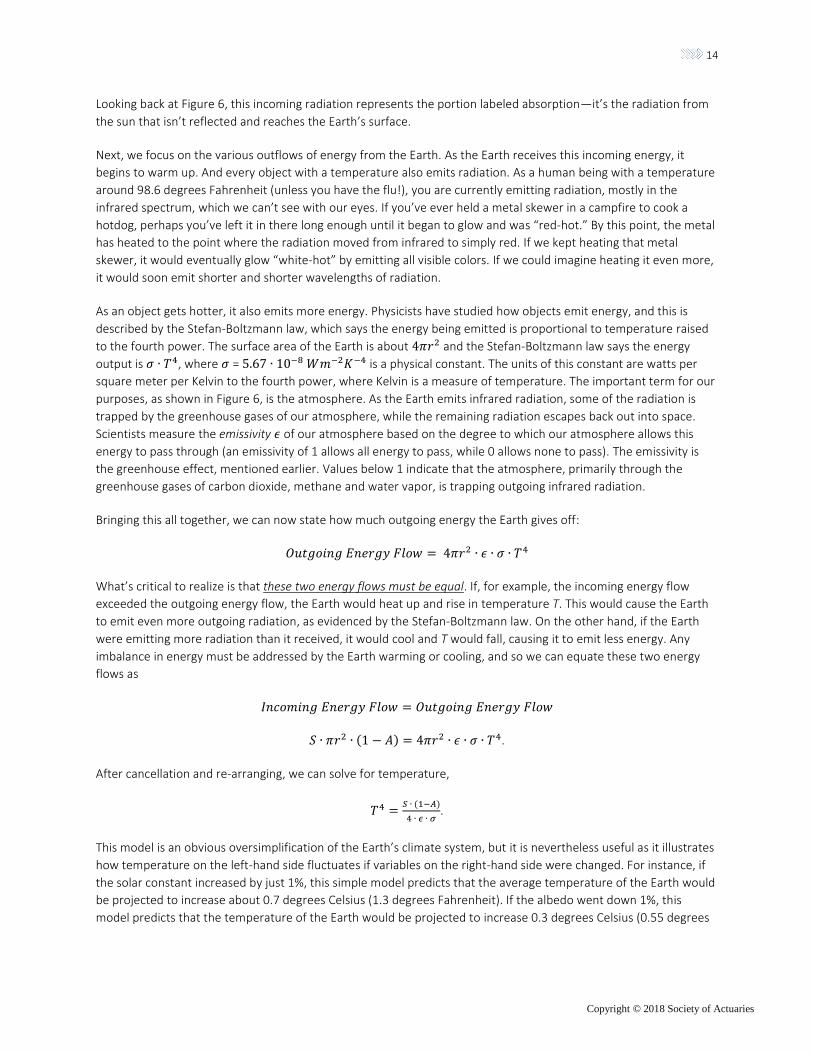
As an object gets hotter, it also emits more energy. Physicists have studied how objects emit energy, and this is

described by the Stefan-Boltzmann law, which says the energy being emitted is proportional to temperature raised

to the fourth power. The surface area of the Earth is about 4𝜋𝑟2 and the Stefan-Boltzmann law says the energy

output is 𝜎 ∙ 𝑇4, where 𝜎 = 5.67 ∙ 10−8 𝑊𝑚−2𝐾−4 is a physical constant. The units of this constant are watts per

square meter per Kelvin to the fourth power, where Kelvin is a measure of temperature. The important term for our

purposes, as shown in Figure 6, is the atmosphere. As the Earth emits infrared radiation, some of the radiation is

trapped by the greenhouse gases of our atmosphere, while the remaining radiation escapes back out into space.

Scientists measure the emissivity 𝜖 of our atmosphere based on the degree to which our atmosphere allows this

energy to pass through (an emissivity of 1 allows all energy to pass, while 0 allows none to pass). The emissivity is

the greenhouse effect, mentioned earlier. Values below 1 indicate that the atmosphere, primarily through the

greenhouse gases of carbon dioxide, methane and water vapor, is trapping outgoing infrared radiation.

Bringing this all together, we can now state how much outgoing energy the Earth gives off:

𝑂𝑢𝑡𝑔𝑜𝑖𝑛𝑔 𝐸𝑛𝑒𝑟𝑔𝑦 𝐹𝑙𝑜𝑤 = 4𝜋𝑟2 ∙ 𝜖 ∙ 𝜎 ∙ 𝑇4

What’s critical to realize is that these two energy flows must be equal. If, for example, the incoming energy flow

exceeded the outgoing energy flow, the Earth would heat up and rise in temperature T. This would cause the Earth

to emit even more outgoing radiation, as evidenced by the Stefan-Boltzmann law. On the other hand, if the Earth

were emitting more radiation than it received, it would cool and T would fall, causing it to emit less energy. Any

imbalance in energy must be addressed by the Earth warming or cooling, and so we can equate these two energy

flows as

𝐼𝑛𝑐𝑜𝑚𝑖𝑛𝑔 𝐸𝑛𝑒𝑟𝑔𝑦 𝐹𝑙𝑜𝑤 = 𝑂𝑢𝑡𝑔𝑜𝑖𝑛𝑔 𝐸𝑛𝑒𝑟𝑔𝑦 𝐹𝑙𝑜𝑤

𝑆 ∙ 𝜋𝑟2 ∙ (1 − 𝐴) = 4𝜋𝑟2 ∙ 𝜖 ∙ 𝜎 ∙ 𝑇4.

After cancellation and re-arranging, we can solve for temperature,

𝑇4 =𝑆 ∙ (1−𝐴)

4 ∙ 𝜖 ∙ 𝜎.

This model is an obvious oversimplification of the Earth’s climate system, but it is nevertheless useful as it illustrates

how temperature on the left-hand side fluctuates if variables on the right-hand side were changed. For instance, if

the solar constant increased by just 1%, this simple model predicts that the average temperature of the Earth would

be projected to increase about 0.7 degrees Celsius (1.3 degrees Fahrenheit). If the albedo went down 1%, this

model predicts that the temperature of the Earth would be projected to increase 0.3 degrees Celsius (0.55 degrees

15


Fahrenheit). And if the emissivity of the atmosphere went down 1%, this model predicts that the Earth would be

projected to increase by 0.7 degrees Celsius (1.3 degrees Fahrenheit).

The purpose of considering this simple model is to see how two quantities, the albedo and the emissivity, relate to

the Earth’s equilibrium temperature through basic physical laws. Neither the solar constant S nor the Stefan-

Boltzmann constant 𝜎 are within our control, so it’s the albedo A and the emissivity 𝜖 that we will focus on as we

seek to understand the Earth’s temperature balance. These quantities, and how humans can influence them, are

described in the next section.

2.2 The Albedo and Emissivity of the Earth

The albedo is the overall measure of reflectivity, and it determines how much solar radiation is sent back into space

without having any heating effect at all. A high albedo means less heat and a cooler Earth, whereas a low albedo

means more heat absorption and a warmer Earth. This is why light-colored roofs are preferable in hot, sunny

regions, such as Arizona.

We saw in the previous section that a simple climate model shows that a 1% reduction in the albedo would mean

about 0.55 degrees Fahrenheit of warming. So why might the albedo A change? Consider Figure 9 below. This

image, from the NASA Goddard Institute for Space Studies, shows the amount of sea ice in the Arctic Circle has been

reduced from September 1979 to September 2015. Ice and fresh snow are highly reflective, and send much of the

incident solar radiation back into space. But when snow and ice melt, the bright white color is replaced by deeper

blues if the ice was in the sea, or by greens and browns if the ice was on land. In both cases, the result is replacing a

highly reflective surface with a less reflective surface that absorbs more heat. Imagine playing soccer on a very hot,

sunny day. If your team’s jersey is white, you are much cooler playing in the sun as you reflect much of the sun’s

energy. But if your jersey is, say, deep ocean blue, you would absorb more heat and feel less comfortable.

Figure 9

Extent of September Sea Ice in the Arctic in 1979 vs. 20157

Source: NASA GISS Visualization Studio 2016. Retrieved May 16, 2018 from

https://www.epa.gov/sites/production/files/styles/large/public/2016-07/arctic-sea-ice-map-figure-2016.png

7 Greenland is the most visible island in the center of each image, with Canada and the Northwest Passage visible on the left side of the image, and Europe and Russia visible on the right.

https://www.epa.gov/sites/production/files/styles/large/public/2016-07/arctic-sea-ice-map-figure-2016.png

16


This change is self-reinforcing. Less ice means less reflectivity, resulting in more absorption of energy and, therefore,

more heat and a higher temperature. This higher temperature then causes more melting ice, less reflectivity, more

heat and so on. This is an example of a positive feedback loop, which accelerates warming.

Changes in the atmosphere’s emissivity also affect climate change. We saw before in our simple climate model that

a 1% reduction in emissivity would result in about 0.7 degrees Celsius (1.3 degrees Fahrenheit). To recognize the

emissivity of the atmosphere, we need to understand the chemistry of our atmosphere. The Earth’s atmosphere is

made up of various gases. Nitrogen gas is by far the most common, comprising 78% of the atmosphere. Oxygen is

around 21%, and argon is just shy of 1%. These three gases compose nearly 100% of our atmosphere. The

remainder is made up of carbon dioxide (0.04%), methane and various other trace gases that occur in smaller

amounts. Carbon dioxide and methane have particular heat-trapping properties, hence scientists describe them as

greenhouse gases. Because the amount of these trace gases is relatively small, scientists often speak about their

concentration in parts per million. At 0.04%, carbon dioxide is around 400 parts per million; methane has a

concentration of around 1.79 parts per million.

These gases have different chemical properties, but each one is very good at absorbing the energy from certain

wavelengths of solar radiation and very poor at absorbing others. Revisit Figure 7. The ultraviolet wavelengths are

just to the right of visible light. Our atmosphere tends not to absorb these, which is why we are prone to sunburns if

we stay outside in the sun for very long—these rays often pass right through our atmosphere. But, our atmosphere

is much better at absorbing the infrared wavelengths, which are just to the left of visible light. This means that our

atmosphere allows much of the incoming solar radiation to pass right through, and that energy is absorbed by the

Earth. But our atmosphere tends to hold on to the outgoing infrared radiation the Earth then emits. The

atmosphere, then, functions as a “blanket,” trapping heat.

Over 100 years of basic chemistry experiments dating back to Swedish chemist Svante Arrhenius’s original

observations from late 1800s confirm the existence of the greenhouse effect. A greenhouse is essentially a glass

house that allows incoming solar radiation to pass through the windows, but tends to absorb the outgoing infrared

radiation and holds on to this energy as heat. Thus, a greenhouse is able to create a warmer space by allowing

incoming energy to enter and holding on to outgoing energy. As the concentration of methane and carbon dioxide

changes, the atmosphere’s ability to hold on to outgoing infrared energy changes, trapping even more energy in the

atmosphere. Understanding this, Arrhenius did a few calculations and predicted that a doubling of CO2 would lead

to about 5–6 degrees Celsius of warming (Arrhenius 1896).

Figure 10 shows a reconstruction of atmospheric carbon dioxide levels from NASA, dating back 400,000 years (left

side) to the present time (right side). Carbon dioxide levels, as the graph shows, fluctuate due to a variety of causes,

including volcanic eruptions, changes in plant biomass from good to poor growing seasons, and other natural

causes. Since around the mid-20th century, however, humans have become very skilled at adding carbon dioxide to

the atmosphere primarily through the burning of fossil fuels such as coal, oil and natural gas. Human-caused

contributions of carbon dioxide are known as anthropogenic greenhouse gas emissions, and these are distinguished

from other non-human contributions.

17


Figure 10

CO2 Levels Over the Past 400,000 Years8

Credit: Vostok ice core data/J.R. Petit et al.; NOAA Mauna Loa CO2 record. Source: Retrieved May 16, 2018 from

https://climate.nasa.gov/system/downloadable_items/43_24_g-co2-l.jpg

Changes in greenhouse gas emissions can change the chemical composition of our atmosphere, which can impact

our atmosphere’s emissivity, which can change the Earth’s temperature. Indeed, carbon dioxide and the

atmosphere’s emissivity is now thought to be the central explanation of why the Earth’s climate system is warmer

since the beginning of the 20th century.

8 NASA created this reconstruction of the concentration of carbon dioxide in our atmosphere (measured in parts per million) dating back 400,000 years. Scientists are able to determine past carbon dioxide levels through a variety of techniques, the most common of which is to measure levels in bubbles trapped in ice within glaciers.

https://climate.nasa.gov/system/downloadable_items/43_24_g-co2-l.jpg

18


Section 3: Climate Model Projections

3.1 General Circulation Models (GCMs) and the Coupled Model Intercomparison Project 5 (CMIP5)

Figure 5 demonstrates the important distinction between weather and climate—namely, that climate is the

distribution of weather. Many actuaries are familiar with weather models and weather prediction from their daily

encounters with them as short-term weather forecasts. Weather models are high-resolution, limited-area

predictions of the weather in the short term. Most people care about temperature, precipitation and perhaps wind

speed, but these variables are related to others such as air pressure, cloud cover and solar radiation. Therefore,

weather models may take into account these background variables. Weather models generally do not try to model

the ocean and instead impose some sort of boundary condition.

Scientists have worked out a series of partial differential equations that relate weather variables to one another in

space and time. These equations include the Navier-Stokes equations, which describe fluid flows; prognostic

equations, which describe the computation of weather variables ahead in time given values through the present;

and diagnostic equations, which describe the relationships between weather variables that occur concurrently in

time. The limited space where the weather will be predicted is often discretized into grid cells with a fine spatial

resolution, and time is discretized into fixed, discrete intervals (for example, in units of 15 minutes). The system of

partial differential equations is solved numerically then, only at the centers of each grid cell and only at the fixed

time points. So long as the grid cells and time steps are sufficiently small and precise, and the full system of

discretized partial differential equations is comprehensive enough to accurately summarize the physics, the

forecasts are reliable. For such weather predictions, it is essential to get the starting conditions correct, namely the

weather state right now, along with the weather in the recent past. Many of the largest discrepancies between two

weather predictions come from slight variations in the starting conditions, rather than disagreements about the

partial differential equations guiding the prediction. A final point about weather prediction: The accuracy is good on

very short time scales such as a few hours and the predictions retain some usefulness out a few days, but there is

virtually no value to weather predictions going further than, say, 10 days into the future because the initial weather

condition right now has virtually no statistical connection to the weather 10 days from now.

However, what if the goal wasn’t to predict the weather at a future time point, but rather to predict the distribution

of weather at that future time point? That is, what if the goal was to describe not the weather but the climate at the

future time period? This is in fact a much easier task. Imagine it is July 1, and you wish to predict the climate for the

upcoming New Year’s Day in New York City. A sensible starting point might be to gather all historical temperature

data from, say, Dec. 15 through Jan. 15 over the previous 10 years, and use those data to estimate the distribution.

A simple histogram of these data would approximate the climate nicely. And as a very crude “prediction” of what

you might actually expect six months from now, you could simply take the mean of this distribution. If you’ve ever

looked at average temperature guides for locations you plan to travel to in order to get an idea of what sort of

weather to expect, you’ve engaged in exactly this process. And so, it can be possible to estimate the future climate

even if it’s impossible to predict the future weather.

This is the goal of climate models. They aim to estimate the distribution of possible weather at future time points.

The most important thing to understand right from the start is that while climate models actually simulate weather,

the goal of doing so is only to capture the correct distribution of weather over long time periods or large spatial

regions. The goal is not to simulate the weather for any limited area or any limited time period, and not to interpret

those simulations as predictions having any reliability. Even the very best climate models are therefore only useful

when one analyzes their projections over large time periods and/or large spatial domains. Many have misused

climate models by ignoring this very simple warning.

19


The climate models used to project forward the Earth’s climate and to study consequences of greenhouse gas

emissions are called general circulation models (GCMs). The first common type is an atmosphere general circulation

model (AGCM), which models the complex physics and chemistry of the atmosphere (specifically, it solves the

Navier-Stokes fluid equations on a rotating sphere, with allowances for heat transfer). These models often model

the variables of pressure, temperature, water vapor, solar radiation, convection, albedo of the earth, cloud cover

and other atmospheric variables in both diagnostic and prognostic equations to properly capture the dynamics of

the atmosphere. A second type of GCM is the ocean general circulation model (OGCM), which models the ocean by

including equations with variables for water temperatures at various depths, sea ice and others features specific to

ocean dynamics. For both AGCMs and OGCMs, the solutions to the set of partial differential equations are found on

discretized sets of grid cells and at discrete time points. These grid cells cover the surface of the Earth, and then are

arranged in layers stretching from the surface to the upper atmosphere. Since the model is being run for the entire

globe and for periods of time stretching decades, the spatial resolution is much lower for climate models than for

weather models (for many AGCMs, grid cells are around 100–150 km near the mid latitudes). Since some

atmospheric processes such as cloud cover or convection occur at scales much smaller than this spatial resolution,

these processes are incorporated into the model through model parameters that need to be set (Berner et. al.

2017). Basic understandings of the climate demonstrate that the ocean influences the state of the atmosphere, and

the atmosphere influences the ocean. To combine these effects, scientists incorporate an AGCM and an OGCM into

a coupled AOGCM. AOGCMs simultaneously solve the systems of equations for atmospheric and oceanic models,

and therefore produce more sophisticated projections.

There is one particular variable in these models that is of central importance to climate model projections, the so-

called carbon emissions scenario under which the model is run. Given the 100+ years of published scientific research

on the greenhouse effect linking atmospheric greenhouse gases to the emissivity and heat-trapping properties of

our atmosphere, Moss et. al. (2010) describes the motivation for and formation of four representative concentration

pathways (RCPs), which are in widespread use across climate models and scientific agencies. As their name

suggests, RCPs are representative of one possible pathway that our planet takes through the year 2100. They

describe a pathway, or trajectory, of atmospheric carbon dioxide levels from the present time through the year

2100, allowing for the possibility of changes in mitigation or social policies in response to a changing climate. They

are not intended as predictions of what scientist expect will happen through year 2100; rather, they are four

possible scenarios that span from a rapid coordinated global response that limits carbon dioxide levels to a scenario

of accelerating carbon dioxide without any sign of stabilization by year 2100. The names of the four scenarios each

take a number (8.5, 6.0, 4.5 and 2.6) that stands for the radiative forcing, or the measured impact on warming, the

particular carbon dioxide pathway would yield. Summaries of the four pathways are shown in Table 1. More

information on their specific formations can be found in a special issue of Climatic Change (Van Vuuren et. al. 2011),

or in Van Vuuren et. al. 2007, Clarke et. al. 2007, Smith and Wigley 2006, Wise et. al. 2009, Fujino et. al. 2006,

Hijioka et. al. 2008, and Riahi, Gruebler and Nakicenovic 2007.

Table 1

Description of the Four Representative Concentration Pathways for Climate Models

Name Radiative Forcing Concentration Pathway

RCP8.5 >8.5 𝑊 ∙ 𝑚−2 in year 2100 >1370 CO2 equivalent in year 2100, rising

Rising

RCP6.0 ~6.0 𝑊 ∙ 𝑚−2 in year 2100 ~850 CO2 equivalent in year 2100, stable

Stabilization

RCP4.5 ~4.5 𝑊 ∙ 𝑚−2 in year 2100 ~650 CO2 equivalent in year 2100, stable

Stabilization

RCP2.6 Peaks at ~3 𝑊 ∙ 𝑚−2 before year 2100, then declines

Peaks at ~490 CO2 before year 2100, then declines

Peak, then decline

Source: Author, with information drawn from Moss et. al. (2010).

20


The Coupled Model Intercomparison Project (CMIP5; https://pcmdi.llnl.gov/mips/cmip5/index.html) is a coordinated

effort organized through the World Climate Research Programme (WCRP) to harmonize certain aspects of the

development and running of GCMs across scientific agencies and countries. This effort is partly to ensure certain

standards regarding variable names, units and model output formatting are common across models, much like

common accounting standards allow for comparisons across companies and nations. But CMIP5 also provides

coordination to “provide a multimodal context” (Taylor, Stouffer and Meehl 2012), which creates the possibility of

investigating a set of scientific questions. These include questions about feedbacks in climate models, predictive

accuracy of model projections on the time scale of decades, and an exploration of why similarly forced models

might produce a range of outcomes. CMIP5 also described and enforced the use of the four RCPs described earlier

and in Table 1, so each scientific agency would run its model under identical scenarios of carbon dioxide levels. A set

of model runs for the same time period and run under the same RCP assumption is called an ensemble, and the

ensemble gives important information about the uncertainty and reliability of the climate projections. Appendix A

lists the GCMs, with the five columns showing the historical runs, as well as future runs through 2100 for each of the

four RCPs.

Scientists use these GCMs to make general claims about the global climate. Figure 11, which comes from the IPCC

Fifth Assessment Report, shows what AOGCMs project for average global land winter temperatures. The horizontal

axis shows time from 1900–2100. A thin solid line represents the average temperature from a single AOGCM run.

From 1900 to about 2010, the individual model runs are each shown as thin gray lines and form an envelope of

results. The heavy black line in the middle of this envelope represents the mean taken across this ensemble.

Appendix A tells us that there are 42 individual AOGCM results in this ensemble. Moving forward in time, each thin

line represents an AOGCM run through year 2100 under one of the four RCPs (red is RCP8.5, orange is RCP6.0, cyan

is RCP 4.5, blue is RCP2.6). Again, Appendix A tells us there are 39, 25, 42 and 32 members of each ensemble. For

each ensemble, a thick colored line shows the mean of all members. To the right of the figure are boxplots taken

across each of the four ensembles, over the period of 2081–2100. These boxplots show the mean and the variability

within each ensemble to give a sense of the reliability/uncertainty of that mean.

https://pcmdi.llnl.gov/mips/cmip5/index.html

21


Figure 11

IPCC Example of How the Ensemble of GCM Runs is Used10

Source: (IPCC 2013c) Figure AI.1 p. 1316

3.2 Results from the IPCC Fifth Assessment Report

Figure 11 demonstrates the individual GCMs, ensembles, means and computation of uncertainty of each ensemble

mean. However, these results only reflect changes in winter temperatures over land. To explore global changes in

mean temperature for all seasons and across the entire surface of the planet, see Figure 12. Figure 12 shows the

four ensembles in expected order, with RCP8.5 showing the largest projected warming (about +4 degrees Celsius by

2100), with RCP 6.0 and RCP4.5 following, and RCP 2.6 projecting about +1 degree Celsius by 2100. The solid

envelopes indicate one standard deviation taken over the ensembles, and the number of model runs comprising

each ensemble are shown. It is clear from such a figure that the variability across RCPs is large when compared to

the interensemble variability within any particular RCP. It is clear that all climate models replicate a narrow envelope

capturing the slight warming observed since around 1950, and it is clear that the scenarios order in precisely the

way one would expect given the known chemistry of the greenhouse effect. Such a figure is one of the major pieces

of evidence that leads the IPCC (IPCC, 2014c) to claim:

Anthropogenic greenhouse gas emissions have increased since the pre-industrial era, driven largely by economic and population growth, and are now higher than ever. This has led to atmospheric concentrations of carbon dioxide, methane and nitrous oxide that are unprecedented in at least the last 800,000 years. Their effects, together with those of other anthropogenic drivers, have been detected throughout the climate system and are extremely likely to have been the dominant cause of the observed warming since the mid-20th century.

10 Individual GCM runs are shown as thin lines, and the color of the line corresponds to which of the four emissions scenarios the model utilizes. The thick lines of the same color are the (pointwise) means across all ensemble members. Thus, the thick lines capture the mean behavior of the emissions scenario, and the width and variability of the ensemble is used as a measure of uncertainty.

22


Figure 12

Global Average Surface Temperature Change11

Source: IPCC Fifth Assessment Report (IPCC, 2013b) Figure SPM.7 on p. 21.

The IPCC Fifth Assessment Report goes well beyond figures showing projected changes in global mean

temperatures. Consider figures 13 and 14, which are formatted much like Figure 12 but show projected changes in

sea level and ocean acidity. Sea levels are expected to rise with warming due to the melting of land ice as well as the

thermal expansion of water (warmer water takes up a larger volume than colder water). Ocean acidification results

from more dissolved carbonic acid as a result of more carbon dioxide in the atmosphere. Once again, the RCPs line

up as expected and variability across scenarios is large compared with variability within.

Figure 13

Projected Sea Level Rise


11 The left side shows hindcasts of the climate models (listed in Appendix A). The right side shows projections forward under each of the four RCP scenarios. For clarity, the envelopes for RCP8.5 and RCP2.6 are shown, which are comprised of 39 and 32 distinct model runs, respectively. The heavy lines show means taken across the ensemble runs. To the far right are means and standard deviations (taken over 2081–2100) for each of the four RCP scenarios. The scenarios order from lowest carbon to greatest carbon, and the difference across RCP scenarios is large compared to the differences within each scenario.

23


Figure 14

Projected Sea Surface Acidity


Figure 11 demonstrates the use of a multimodel ensemble of individual members to produce a distribution of

outcomes meant to incorporate intermodel variability, or the variability across different models. An alternative

quantity is intramodel variability, or an investigation of the variability within a particular model that arises from

uncertainty in the parameters, parameterization, initial conditions and so forth. To explore such variability, a

perturbed physics ensemble is a set of projections for an identical climate model run repeatedly under perturbed

parameterizations, such as those shown in Murphy et. al. (2004). We first describe a subset of this in which one re-

runs identical climate models under different initial conditions to explore the impact starting values have on internal

model variability. This experiment (http://www.cesm.ucar.edu/projects/community-projects/LENS/) was conducted

and is described in great detail by Kay et. al. (2015).

Kay et. al. (2015) write that “internal climate variability is often underappreciated and confused with model error

(e.g., as discussed in Tebaldi, Arblaster and Knutti 2011).” To quantify the impact of initial conditions in internal

model variability, they designed an experiment in which 30 runs from the same GCM Community Earth System

Model Large Ensemble (CESM-LE) were run, but under different initial conditions as starting values. There are

known scientific reasons to suppose that starting values of atmospheric variables have little influence on climate

model runs, as “atmosphere, land and sea ice processes have memory on short time scales (weeks to years), so the

influence of their initial conditions on the coupled climate state in a multicentury-long control simulation is

negligible” (Kay et. al. 2015). The deep ocean, on the other hand, has a longer memory.

Each of the 30 runs was initialized to a different, perturbed initial state on Jan. 1, 1920, and run through 2005 using

observed climate forcings. Forward to 2100, each used the RCP 8.5 pathway as a forcing. Global mean surface

temperatures of the 30 model runs form a tight envelope moving from present day to about +4.75 degrees Celsius

by the year 2100. The spread of this envelope is a mere 0.4 degrees Celsius, and the authors conclude that “internal

variability causes a relatively modest 0.4-K[elvin] spread in warming across ensemble members.” (Note: Changes in

temperature measured in Celsius or Kelvin are identical.) Such a small overall measure of internal variability as a

result of initialization supports the view that initial conditions of climate models are often not of primary concern for

producing reliable projections over long periods.

The results from CESM-LE also have very important implications for the spread in CMIP5 models. The spread in

CMIP5 trend estimates comes from a combination of two sources: internal climate variability (i.e., uncertainty of

individual model runs) and intramodel variability. The authors compare the spread of winter (December-January-

February) temperature trends from the 30 member CESM-LE ensemble to the spread of winter temperature trends

from the full CMIP5 ensemble using the standard deviation of trend estimates (over 34 years) as a measure of

variability, for both the past (1979–2012) and future (2013–46). They find that the spread of trend estimates

http://www.cesm.ucar.edu/projects/community-projects/LENS/

24


between these two groups is very similar across much of the Earth. The “stunning” conclusion is that the spread in

CMIP5 winter temperature trends can be explained by internal climate variability, rather than model differences.

That is, Kay et. al. (2015) demonstrates that the variability in CMIP5 winter trend estimates is overwhelmingly due to

internal climate model variability and not disagreements across model specification. A tool explained in Phillips,

Deser and Fasullo (2014) allows users to further study CESM-LE runs in relation to CMIP5 runs.

Taking a step back, in addition to altering initial conditions, one can modify or perturb the internal parameters of the

models themselves to explore how uncertainty of parameters impacts uncertainty in final projections. The issue was

prominently stated in Allen and Stainforth (2002): “For many variables, however, the main uncertainty in multi-

decadal climate projections is not in the initial state nor in the external driving, but in the climate system’s

response,” by which they meant the internal climate model parameters. Shortly after, an analysis of a 53-member

climate model ensemble constructed by varying internal model parameters whose values “could not be accurately

determined from observations” was published (Murphy et. al. 2004). Using the Hadley Centre Coupled Model

version 3 (HadAM3), the authors identified 29 model parameters (out of just over 100) crucial to subgrid climate

phenomena, and perturbed these parameters to create an ensemble of 53 model versions of the same fundamental

GCM. Their target was an estimate of the climate sensitivity of doubling atmospheric carbon dioxide. They

estimated this using both unweighted (i.e., all 53 members were treated equally) and weighted (i.e., unequal

weights, based on model performance) and found the middle 90% of projections gave a range of (+1.9, +5.3)

degrees Celsius for unweighted, and (+2.4, +5.4) degrees Celsius for weighted. The medians across the 53 runs were

+2.9 and +3.5 degrees Celsius, respectively. The authors noted that this “ensemble produces a range of regional

changes much wider than indicated by traditional methods.” Still, after accounting for this parameter uncertainty,

the range of outcomes was still significantly concentrated in the middle near +3 degrees Celsius, and the range was

strongly separated from 0 degrees Celsius.

A follow-up study was conducted through https://www.climateprediction.net (Stainforth et. al. 2005). The study is a

perturbed physics ensemble of 2,578 simulations all based on the HadAM3 atmospheric model coupled with a

mixed-layer ocean. This massively expensive ensemble was made possible by utilizing spare computing capacity on

90,000 volunteers’ computers. In this ensemble, “model parameters are set to alternative values considered

plausible by experts in the relevant parameterization schemes. Two or three values are taken for each parameter”

and simulations may have multiple parameters perturbed. The distribution of simulated climate sensitivities to a

doubling of atmospheric carbon dioxide span from +1.9 degrees Celsius to +11.5 degrees Celsius due to a very long

tail, but most are clustered around +3.4 degrees Celsius, which is the value of the single unperturbed model run

(only 4.2% above +8 degrees Celsius). The authors suggest that many parameter perturbations combine to have

little impact on the global temperature variable with mutually compensating effects. They do, however, note that

the model spread from this single perturbed physics ensemble is greater than the spread of the CMIP5 ensemble,

which confirms that the ensemble undersamples parameter variability.

The CMIP5 ensemble is designed to sample across parameters and model specifications to capture variability in

outcomes. These two perturbed physics ensemble experiments show that while the CMIP5 ensemble undersamples

parameter variability and therefore understates model variability in outcomes, the magnitude of this understated

variance is not so large as to wash out the climate signals across carbon emissions scenarios. Many perturbed model

runs produce similar warming paths, and the full spread of the ensemble is still noticeably above zero. For more

detail on these parameters and how perturbation impacts model runs, see Hourdin et. al. (2017).

While the compelling results above show strong changes for the entire globe, planning for climate change happens

at far more local levels, and indeed GCMs show strong spatial variation across the globe. The high latitudes have

been warming the fastest and are projected to continue doing so, partly as a result of a strong change in albedo as

white snow and ice melts and is replaced by darker colors. GCMs can be used to produce maps of projected

changes, such as those shown in Figure 15. But even here, the spatial resolution from a model run at coarse grid cell

https://www.climateprediction.net/

25


sizes of 100–150 km cannot produce fine-scale regional projections. To remedy this, the next section will describe

regional climate models (RCMs) and downscaling, both of which produce finer spatial resolution results.

Figure 15

Examples of Changes in Seasonal Averages12

Source: NARCCAP. Retrieved May 16, 2018 from http://www.narccap.ucar.edu/results/seas-delta-maps/index.html. The source of this

material is the University Corporation for Atmospheric Research (UCAR). All rights reserved.

3.3 Regional Climate Models and Downscaling

Figures 2–5 show what has happened in the recent past on average, across the entire globe. Similarly, Figures 11–14

show some projections from the ensemble of CMIP5 general circulation models, but again these projections are for

the entire globe. As mentioned in Section 3.1, we can confidently interpret results of climate by looking at very large

spatial regions or very large time periods. However, the scale at which impacts are assessed and decisions are made

by stakeholders is often not global and decadal; it is local and on shorter time horizons. There is therefore a

fundamental mismatch between the spatial and temporal precision of the projections that GCMs can provide, and

the resolution that decision makers and stakeholders need to assess changes.

If it were possible to simply run GMCs at a very fine spatial resolution, this would be ideal. As grid cells shrink to

smaller sizes, the number of subgrid-scale processes handled through parameterization would also shrink. The

spatial resolution of projections would match the scale stakeholders seek, and grid cells themselves would cover

more homogeneous regions of the Earth rather than extend across a mixture of elevations, ecosystems and

microclimates. However, the computational cost of running climate models on very fine grid cells exceeds what is

currently available from even the very fastest computing clusters. Each division of a grid cell by half increases the

number of cells on a surface by a factor of 4; in three dimensions, halving the spatial scale increases the number of

cells by a factor of 8.

To remedy this, we introduce the concept of downscaling, which is the process by which one takes coarse spatial

projections from GCMs and infers local-scale features of the projections. A now “classic” reference on the subject is

Wilby and Wigley (1997). As an example, consider precipitation. A GCM run at a coarse spatial resolution would only

be able to describe the average precipitation over a very large area, but rainfall is highly localized and it may be that

some locations in the grid cell experience a thunderstorm, while other areas receive no rainfall. A mechanism that

12 Examples are of projected changes in summer (June-July-August) mean temperatures over North America for three different GCM runs. Changes are the average taken over 2041–70 compared to the average taken over 1971–2000.

http://www.narccap.ucar.edu/results/seas-delta-maps/index.html

26


links the large-scale GCM output on precipitation to small-scale, point-referenced local areas would be needed to

utilize GCM output in the study of future precipitation.

In contemporary terms, there are fundamentally two types of downscaling. The first establishes statistical patterns

between coarse GCM output and subgrid cell variables and is known as statistical downscaling. A second approach

seeks to utilize climate models as numeric solutions to systems of partial differential equations and is known as

dynamic downscaling.

Statistical downscaling represents any statistical model that relates GCM output to quantities at a smaller scale

through statistical modeling (Mauran and Widmann 2017). This approach first requires a set of climate model

outputs and also subgrid-cell data for the same time period. A fundamental assumption in statistical downscaling is

that the information needed to downscale is in fact inherent in the climate model data; that is, one assumes there

exists a statistical relationship between large-scale climate model output and small-scale variability that can be

modeled. Although widely used in many applications, particularly in hydrology and for precipitation, statistical

downscaling may not be the most effective choice for actuarial applications. This approach requires a high degree of

climate modeling and statistical expertise.

Dynamic downscaling involves nesting a fine spatial scale regional climate model (RCM) run over a limited area

inside of a coarse spatial scale GCM run everywhere on the globe. The RCM involves precisely the same physical

models of climate variables as the GCM, it is simply run at a much finer spatial (and perhaps temporal) resolution.

The coarse GCM sets the boundary conditions for the limited area regional climate model. This approach then is a

tradeoff between computational complexity and running a climate model at a very fine spatial resolution. The

coarse GCM run everywhere outside the limited area captures large-scale climate effects at a relatively low

computational cost, while the regional climate model inside the limited area captures fine-scale climate effects but

at a much higher computational cost. The fundamental assumption here is that the large-scale climate information

forces (or “drives”) the regional climate information. Close attention to the boundary conditions and interactions is

essential to effective regional climate modeling. See Foley (2010), Giorgi and Mearns (1999), Rummukainen (2010)

and Wang et al. (2004) for general introduction and discussion of RCMs. Dynamic downscaling may be preferred by

actuaries since the end-product RCMs are available to actuaries already and were produced by climate modeling

experts having already considered many of the downscaling issues.

Mirroring the success of coordinating GCMs into CMIP5 with a common basis for comparisons, the Coordinated

Regional Climate Downscaling Experiment (CORDEX; Giorgi, Jones and Asrar 2009) was organized by the World

Climate Research Program Task Force on Regional Climate Downscaling. CORDEX designates eight regions (shown in

Figure 16) over which it provides a common framework for benchmarking and evaluating RCMs, along with a

designed set of experiments to produce ensembles of regional climate model projections. Africa was selected as the

preliminary region used to implement both of these goals. Kim et. al. (2014) performed a comprehensive study of 10

RCMs run over the period of 1990–2007 with identical boundary conditions obtained from historical weather to

judge the bias, variability and intermodel variability of the ensemble. Comprehensive details are provided in the

paper, but they quantify biases in precipitation, temperature, regional differences and so forth. They write that “for

all variables, multimodel ensembles generally outperform individual models included [in the ensemble].”

27


Figure 16

Locations of the Regional Climate Models from CORDEX

Source: Giorgi, Jones, and Asrar (2009). Reprinted with permission from the World Meteorological Organization. Copyright 2009.

In North America, the most comprehensive set of regional climate models is the North American Regional Climate

Change Assessment Program (NARCCAP; www.narccap.ucar.edu. See Mearns et. al. 2009 for background). NARCCAP

runs a set of 50 km spatial resolution RCMs driven by a set of GCMs for both the near past (1971–2000) as well as

the mid-20th century (2041–70). The GCMs are forced with the Special Report on Emissions Scenario (SRES) A2

emissions scenario (see http://www.narccap.ucar.edu/about/emissions.html or Nakicenovic et al. 2000 for more

detail). Each RCM is also nested in National Centers for Environmental Prediction (NCEP) Reanalysis II data, which

uses observed historical climate data from 1979–2004 to drive the RCM, and therefore output from these NCEP

experiments can be compared to actual historical climate to validate and verify the RCM.

Figure 17 describes the four GCMs used to drive RCMs. The GCMs are: the Canadian Centre for Climate Modelling

and Analysis Coupled Global Climate Model version 3 (CGCM3; Flato 2005), the National Center for Atmospheric

Research Community Climate System Model version 3 (CCSM3; Collins et al. 2006), the Geophysical Fluid Dynamics

Laboratory (GFDL) Climate Model version 2.1 (GFDL 2004), and the United Kingdom Hadley Centre Coupled Model

version 3 (HadCM3; Gordon et al. 2000, Pope et al. 2000). Regional climate models include the Canadian Regional

Climate Model (CRCM; Caya and Laprise 1999), the NCEP Regional Spectral Model (ECP2; Juang, Hong and

Kanamitsu 1997), the Hadley Regional Model 3 (HRM3; Jones et. al. 2004), the Pennsylvania State University /

National Center for Atmospheric Research (PSU/NCAR) Mesoscale Model (MM5I; Grell, Dudhia and Stauffer 1993),

the National Center for Atmospheric Research Regional Climate Model version 3 (RegCM3; Pal et al. 2007;

Maintained by the Abdus Salam International Centre for Theoretical Physics (ICTP)), and the Weather Research and

Forecasting model (WRFG; Shamarock et al. 2005).

http://www.narccap.ucar.edu/

http://www.narccap.ucar.edu/about/emissions.html

28


Figure 17

Combinations of Regional Climate Models and Driving Models13

Source: https://www.earthsystemgrid.org/project/NARCCAP.html. The source of this material is the University Corporation for Atmospheric Research (UCAR). All rights reserved.

Figure 18 shows one example of the increased spatial resolution available from the dynamically downscaled RCM

nested within a GCM. Here we see projected changes in average seasonal precipitation in March-April-May from

2041–70 as compared to 1971–2000, using a GCM only (left) and an RCM nested within the same GCM (right).

Figure 18

Example of Projected Change in Seasonal Average Precipitation, March-April-May, in 2041–70 vs. 1971–200014

Source: http://www.narccap.ucar.edu/results/seas-delta-maps/rcm3-cgcm3-results.html. The source of this material is the University

Corporation for Atmospheric Research (UCAR). All rights reserved.

13 These combinations of regional climate models and driving models, which include GCMs, are available in the NARCCAP project. Observe that not every RCM is run within every GCM due to computational cost. 14 Left image shows projected change from the GCM CGCM3 only. Right image shows the projected change from the dynamically downscaled RCM3 nested within the CGCM3 for the same time period and region.

https://www.earthsystemgrid.org/project/NARCCAP.html

http://www.narccap.ucar.edu/results/seas-delta-maps/rcm3-cgcm3-results.html

29


We now take a step back from specific models or regions, and instead ask broad questions about the quality and

utility of such models. Foley (2010) gives a conceptual, philosophical overview of the various forms of uncertainties

present within regional climate models. Uncertainty in the emissions scenarios is named the “greatest uncertainty”

in climate modeling, but one that covers a range of plausible futures despite not covering all eventualities. Also

discussed are uncertainty in climate sensitivity (change in response to climate forcings), natural variability, and

feedbacks or surprises. For each of these, the degree to which any are truly knowable or predictable is honestly

questioned. As a result, one may reasonably ask to what degree regional climate model outputs are useful for

particular purposes. The answer to this must involve a careful treatment of uncertainty. Two broad methods of

using climate models to produce a range of scenarios incorporating as much uncertainty as possible are perturbed

physics ensembles and multimodel ensembles. We discuss each briefly, then describe what researchers have found

by using both.

Perturbed physics ensembles involve taking a single regional climate model and re-running it under slightly different

parameterizations across a well-designed range of inputs meant to span the range of what scientist believe is the

uncertainty in those parameter estimates. Such a computer experiment could fully demonstrate the range of

outcomes and thus climate uncertainty, which arises from uncertainty in the parameter estimates themselves; some

of these experiments are conducted. As stated in Foley (2010): “Due to the time and computer resource constraints

associated with regional modelling and the limitations of computing standards, it is just not feasible to produce RCM

ensembles of similar size to the current crop of GCM ensembles.”

Multimodel ensembles represent the other primary means of using regional climate models to produce a range of

scenarios incorporating uncertainty. This approach—already shown in Figure 11 and underlying the construction of

figures 12, 13 and 14—uses intermodal variability to represent the spread of projections, but as pointed out in Foley

(2010), such an approach also helps to account for intramodel variability in that a more complete range of inputs,

parameterizations and so forth is utilized as each RCM differs in these respects. There is a distinction between

validation of a model, that it meets suitable performance standards for particular uses, and verification of a model,

that it matches a ground truth of the real climate. This distinction becomes particularly important in this context of

multimodel ensembles: An ensemble constructed of individually validated models each achieving high scientific

standards can be used to explore a range of future climate scenarios, even if individual members differ to such a

degree that verification of every member is not realistic.

As described earlier, RCMs can be run for the future when nested inside a GCM, or they can be run for the recent

past and driven either by a GCM also run for the past, or a re-analysis product, which is essentially using the

observed, historical climate as the driving force. Runs for the recent past are sometimes termed hindcasts, and they

allow scientists to investigate the degree of correspondence between model output and observed, historical climate

features. Dynamically downscaled RCMs designed to address regional climate questions are only useful if they

exhibit some benefit over coarse GCMs, if they can be validated as described above, and if their hindcasts show an

appropriate correspondence to observed climate features.

To the first point, Feser et. al. (2011) shows RCMs add value to the GCMs they were built from. The authors analyze

RCM hindcasts driven by reanalysis data, and use a common measure called the Brier skill score to assess how well

the hindcasts capture distributions of climate variables. They conclude: “RCMs do indeed add value to global models

for a number of applications, variables and areas. If examined only at the regional scale, added value emerges very

distinctly for many model variables, justifying the additional computational effort of RCM simulations.”

A number of studies have explored RCM hindcast performance further. Bergant, Belda and Halenka (2007) explores

the performance of the RegCM3 climate model over Europe, for the period 1961–2000, and compare distributional

features of the climate model hindcast to observed climate data obtained from the Climate Research Unit (CRU).

After exploring a number of variables across Europe, the authors conclude that the “overall relatively good

30


performance of RegCM3” makes it a “valuable tool in the regional projection of future climate change.” Jacob et. al.

(2007) expands to study an ensemble of nine different RCMs, each driven by the same GCM forcing over Europe.

These models are a part of a project known as PRUDENCE (Prediction of Regional scenarios and Uncertainties for

Defining EuropeaN Climate change risks and Effects; Christensen and Christensen 2007). Again using hindcasts over

Europe but for 1961–90, the authors quantify biases in temperature and precipitation in both summer (June-July-

August) and winter (December-January-February) over nine regions in Europe. They conclude that the RCMs run

warmer relative to observed climate in winter and summer, but a bit cooler in fall and spring. Biases in mean

temperature fall in the range of (±3 Celsius) but are often much lower for some regions and models.

An ensemble of nine NARCCAP RCMs driven by a variety of GCMs is analyzed in Kabela and Carbone (2015) over the

southeastern United States for the period 1970–99. The authors consider two regions “east” (NC, SC < GA) and

“west” (TN, AL, MS) and use a variety of measures to assess the degree of correspondence between hindcasts and

observed climate, including the Perkins skill score (Perkins et. al. 2007), Willmott’s index of agreement (Willmott,

Robeson and Matsuura 2012, root-mean-square error (RMSE) and mean absolute error (MAE) of sorted daily values

by month, and model bias in percentiles following Kjellstrom et. al. (2010). These are applied to distributions of

maximum temperature, minimum temperature and daily precipitation. Crucially, each measure compares

distributions of these variables, as the purpose and function of NARCCAP climate models is to capture the

distribution of climate variables, rather than to predict accurately for any particular day. Model performance across

variables and regions is mixed, though the authors conclude that “most models demonstrated high skill for

maximum and minimum temperature” and that “all models reproduce daily minimum temperature trends relatively

skillfully.” Precipitation skill varies more, with high skill for the probability distribution measures but lower skill with

RMSE of MAE due to a tendency of RCMs to overestimate the frequency of extreme precipitation events.

The existence of biases in an RCM’s ability to reproduce distributions of historical climate simply motivates the need

for bias correction and a further statistical downscaling step when utilizing RCM output. For example, if an RCM ran

everywhere warms by 1 degree Celsius for the historical period, one could assume that bias is preserved in future

runs and simply subtract 1 degree Celsius from the future RCM runs. Likewise, if an RCM overstated variability of

precipitation in the historical period, one could quantify this bias and apply that adjustment to future model runs.

This requires the assumption that the bias holds through the future period. Mauran (2016) and Mauran and

Widmann (2017) discuss this sort of bias correction, and the follow-up paper to this white paper by Jin and Erhardt

demonstrates these corrections using NARCCAP models.

Despite known limitations and challenges, global and regional climate models are essential for decision makers.

Historical data alone are not enough, as noted in Foley (2010): “In a system undergoing change, past observations

are unlikely to be a robust estimator of future behavior. … Therefore, long-term projections from climate models are

needed to determine likely changes on which to base adaptive planning.” The uncertainties in regional climate

models are numerous, but they can be minimized, quantified and communicated in such a way that allows decision

makers to consider plausible future scenarios. Kay et. al. (2015) remind us: “While the comparison of models and

observations provides important insights, climate change projections are made in part to plan for a future we

cannot observe.”

31


Section 4: Conclusion

In this paper, we have described the necessary background on climate science, global climate projections, and

general circulation and regional climate models to help the actuary become conversant and literate in the major

tools available for climate change projections. Better utilizing these tools for actuarial work is the next task for the

insurance industry to be better prepared to address climate change and its effect on risk assessment.

Actuaries already utilize several variables included in climate models, including wind speed, precipitation and

temperature. Each is used in various index-based insurance products, and each can be used in statistical models

relating these quantities to estimates of flood, wind damage, heatwaves, events leading to crop losses, mortality

risks and other loss scenarios. Regional climate models project how distributions of these quantities may shift over

time for a given climate change scenario, along with dozens of other variables. Therefore, actuaries could enhance

existing models and estimates with regional climate model output.

Many recent papers have quantified links between climate change and human health or mortality. A few

representative papers include Crimmins et. al. (2016), Luber et. al. (2014), Ebi et. al. (2017), Frumkin et. al. (2008),

Bell et. al. (2016), LaKind et. al. (2016) and Mitchell et. al. (2016). But for health and life insurers, it may be the case

that climate change impacts on regulation or investments has the stronger impact on their business—see, for

example, National Association of Insurance Commissioners (2008), Messervy, McHale and Spivey (2014) or United

Nations Environment Programme Finance Initiative (2006).

A more direct link between weather variables and insurance products can be found in index-based insurance,

weather derivatives, temperature derivatives and related products. Each of these involve a contract that specifies a

weather station or stations, weather variables of interest, a payment structure between parties contingent upon

specific weather outcomes, and a time period over which the contract is in force. For weather outcomes that might

lead to financial loss (for example, high wind speeds leading to coastal property damage, low rainfall leading to crop

loss, very high or very low temperatures leading to high energy use), one can define payments that would be

triggered by such weather events. The Munich Climate Insurance Initiative (http://www.climate-

insurance.org/home/) described the “Livelihood Protection Plan” with weather derivatives paying residents of the

Caribbean in the event of very high wind speeds or very heavy precipitation, since both are strongly associated with

property damages. Given the direct link between weather and the payments, models for the weather directly inform

models for payments and thus allow for actuarial pricing based on the distribution. A few references on these

products or examples of incorporating climate trends into their analysis can be found in Geman (2001), Jewson and

Brix (2005), Zeng (2000) and Erhardt (2015).

The forthcoming follow-up paper, “Incorporating Climate Change Projections into Risk Measures of Index-Based

Insurance” by Zhouli Jin and Robert Erhardt, demonstrates the use of regional climate model data for the purposes

of estimating actuarial risks of index-based temperature insurance in California. The paper uses an ensemble of six

GCM/RCM combinations—(1) the Canadian Regional Climate Model nested within the Community Climate System

Model (CRCM-CCSM); the (2) Canadian Regional Climate Model nested within the third generation Coupled Global

Climate Model (CRCM CGCM3); the (3) Weather Forecasting Research Group model nested within the Community

Climate System Model (WRFG-CCSM); the (4) Weather Forecasting Research Group model nested within the third

generation Coupled Global Climate Model (WRFG-CGCM3); the (5) the Hadley Regional Model 3 nested within the

Hadley Centre Coupled Model, version 3 (HRM3-HadCM3); and the (6) PSU/NCAR Mesoscale Model nested within

the Hadley Centre Coupled Model, version 3 (MM5I-HadCM3). All model combinations are freely available at

NARCCAP and discussed at http://www.narccap.ucar.edu/data/model-info.html. Regional climate model hindcasts

(1971–2000) are first compared to historical temperature data obtained from the National Centers for

Environmental Information to identify any needed bias and variance corrections. These corrections are then applied

http://www.climate-insurance.org/home/

http://www.climate-insurance.org/home/

http://www.narccap.ucar.edu/data/model-info.html

32


to regional climate model projections of future (2041–70) temperature in California. Thus, the paper demonstrates

the use of both dynamic downscaling through the regional climate model as well as statistical downscaling through

bias and variance corrections. Downscaled future climate model output from the ensemble are used to construct

distributions of cumulative cooling degree days, a key quantity used in temperature risk, and from these payments

of hypothetical temperature derivatives are computed and analyzed. The computer code for obtaining,

manipulating and analyzing all data was written in R and will be made freely available using the following link:

http://users.wfu.edu/erhardrj/.

This paper has described the major physical forces that shape our climate, the ways in which scientists understand

and model those forces at the global scale, and how they refine their models for the regional scale, while keeping an

eye on probabilistic modeling of scenarios and known hazards for risk modeling. The goal of this paper is to build

scientific literacy among the readers, allowing them to understand anthropogenic influences on climate change and

further understand how scientists work to translate those influences into future projections of possibilities.

Projections are not predictions. And natural forces are also at play alongside anthropogenic ones. The Earth’s

climate oscillates according to non-anthropogenic forces such as El Nino-Southern Oscillation, thermohaline

circulation, the Earth’s precession, and so forth. However, observed increases in greenhouse gas concentrations

from documented human sources, along with the basic science linking these gases to warming, means an overall

anthropogenic climate trend is superimposed on all other natural forces. The scientific consensus is that this

anthropogenic trend is the dominant driver of observed climate change. Stern (2006) points out that the cost of

inaction is likely to be far greater than the cost of early action. Despite the persistence of various forms of

uncertainty in global and regional climate models, their proper use presents actuaries opportunities to better

measure and manage the growing climate risks across the industry.

http://users.wfu.edu/erhardrj/

33


Acknowledgments

The authors wish to thank the Society of Actuaries Research Expanding Boundaries (REX) Funding Pool for their generous financial support of this project. The authors further wish to thank Scott Lennox and Erika Schulty at the SOA for their leadership and guidance, and the volunteers who formed the Project Oversight Group. All provided valuable perspectives and feedback, which strengthened this paper.

34


Appendix A: The Construction of the Historical Temperature Record (Figure 3)

The historical record for land and sea surface temperatures from 1880–present is based on two data sets. Land

measurements come from the Global Historical Climate Network-Monthly (GHCN-M;

https://www.ncdc.noaa.gov/ghcnm/), and sea surface temperatures are obtained from reconstructions based

ultimately on the International Comprehensive Ocean-Atmosphere Data Set (ICOADS; http://icoads.noaa.gov/). Each

are first summarized into monthly, 5 degree by 5 degree grid cells (Smith et al. 2008).

For complete references on the construction of the data set used to compute anomalies, see Peterson and Vose (1997), Quayle et. al. (1999), Smith and Reynolds (2004), Smith and Reynolds (2005), Smith et. al. (2008) and Huang et. al. (2015); for details on the Climate Research Unit’s complete land-sea surface climatology, see Jones et. al. (1999); for more information on data for land areas, see Parker, Jackson and Horton (1995); and for information regarding how sparse temperature measurements over Antarctica were handled, see Rigor, Colony and Martin (2000) and Martin and Munoz (1997).

Below are a few relevant citations taken from NOAA (https://www.ncdc.noaa.gov/monitoring-references/faq/anomalies.php) that provide additional information and references on the data set construction.

“Sea surface temperatures are determined using the extended reconstructed sea surface temperature (ERSST)

analysis. ERSST uses the most recently available International Comprehensive Ocean-Atmosphere Data Set (ICOADS)

and statistical methods that allow stable reconstruction using sparse data. The monthly analysis begins January

1854, but due to very sparse data, no global averages are computed before 1880. With more observations after

1880, the signal is stronger and more consistent over time.”

“Effective June 2015, the GHCN-M version 3.3.0 data set of monthly mean temperature replaced the GHCN-M

version 3.2.2 [https://www1.ncdc.noaa.gov/pub/data/ghcn/v3/techreports/Technical%20Report%20NCDC%20No12-

02-3.2.0-29Aug12.pdf] monthly mean temperature data set. Beginning with the May 2015 Global monthly State of

the Climate Report, released on June 18, 2015, GHCN-M version 3.3.0 is used for NCEI climate monitoring activities,

including calculation of global land surface temperature anomalies and trends. For more information about this

newest version, please see the GHCN-M version 3.3.0 Technical Report

[https://www1.ncdc.noaa.gov/pub/data/ghcn/v3/techreports/Technical%20Report%20GHCNM%20No15-01.pdf].”

“ERSST version 4 is currently used. Version 4 of the ERSST data set improves or corrects for several factors related to sea-surface temperature (SST) measurements. These include: updated and substantially more complete input data from ships and buoys, improved metadata associated with these observations, updated SST quality control procedures, revised SST anomaly evaluation methods, updated corrections to ship SSTs using nighttime marine air temperature, accounting for differences inherent in buoy (relative to ship-borne) observations, and improved methods of identifying and using persistent statistical relationships between neighboring regions to help validate observations and address missing data. Complete information on these changes is available in Huang et al. (2015).”

“The global time series is produced from the Smith and Reynolds blended land and ocean data set (Smith et al. 2008). This data set consists of monthly average temperature anomalies on a 5 [degree] x 5 [degree] grid across land and ocean surfaces. These grid boxes are then averaged to provide an average global temperature anomaly. An area-weighted scheme is used to reflect the reality that the boxes are smaller near the poles and larger near the equator. Global-average anomalies are calculated on a monthly and annual time scale. Average temperature anomalies are also available for land and ocean surfaces separately, and the Northern and Southern Hemispheres separately. The global and hemispheric anomalies are provided with respect to the period 1901–2000, the 20th century average.”

https://www.ncdc.noaa.gov/ghcnm/

http://icoads.noaa.gov/

https://www.ncdc.noaa.gov/monitoring-references/faq/anomalies.php

https://www.ncdc.noaa.gov/monitoring-references/faq/anomalies.php

https://www1.ncdc.noaa.gov/pub/data/ghcn/v3/techreports/Technical%20Report%20NCDC%20No12-02-3.2.0-29Aug12.pdf

https://www1.ncdc.noaa.gov/pub/data/ghcn/v3/techreports/Technical%20Report%20NCDC%20No12-02-3.2.0-29Aug12.pdf

https://www1.ncdc.noaa.gov/pub/data/ghcn/v3/techreports/Technical%20Report%20GHCNM%20No15-01.pdf

35


Appendix B: Names and Number of GCMs for Each RCP Run (IPCC AR5)

Source: IPCC Fifth Assessment Report (IPCC 2013c). Table AI.1 p. 1315.

36


References Alberts, Mark. 2017. Climate Sources for Actuaries. Schaumburg, IL: Society of Actuaries. https://www.soa.org/research-reports/2017/2017-climate-sources-actuaries/.

Allen, Mark R., and David A. Stainforth. 2002. “Towards Objective Probabilistic Climate Forecasting.” Nature 419, no. 6903: 228.

Arrhenius, Svante. 1896. “On the Influence of Carbonic Acid in the Air Upon the Temperature of the Ground.” Philosophical Magazine and Journal of Science 41, no. 251: 237–76.

Bell, Jesse E., Stephanie C. Herring, Lesley Jantarasami, Carl Adrianopoli, Kaitlin Benedict, Kathryn Conlon, Vanessa Escobar, et al. 2016. “Impacts of Extreme Events on Human Health.” Chap. 4 in The Impacts of Climate Change on Human Health in the United States: A Scientific Assessment. Edited by A. Crimmins, J. Balbus, J. L. Gamble, C. B. Beard, J. E. Bell, D. Dodgen, R. J. Eisen, et al. Washington, D.C.: U.S. Global Change Research Program. https://doi.org/10.7930/J0BZ63ZV.

Bergant, Klemen, Michael Belda, and Tomas Halenka. 2007. “Systematic Errors in the Simulation of European

climate (1961–2000) with RegCM3 Driven by NCEP/NCAR reanalysis.” International Journal of Climatology 27, no. 4:

455–72.

Berner, Judith, Ulrich Achatz, Lauriane Batte, Lisa Bengtsson, Alvaro de la Camara, Hannah M. Christensen, Matteo Colangeli, et al. 2017. “Stochastic Parameterization: Toward a New View of Weather and Climate Models.” Bulletin of the American Meteorological Society 98, no. 3: 565–88.

Caya, Daniel, and Rene Laprise. 1999. “A Semi-Implicit Semi-Lagrangian Regional Climate Model: The Canadian RCM.” Monthly Weather Review 127, no 3: 341–62 Chen, J. L., C. R. Wilson, and B. D. Tapley. 2013. “Contribution of Ice Sheet and Mountain Glacier Melt to Recent Sea Level Rise.” Nature Geoscience 6, no. 7: 549–52.

Christensen, Jens Hesselberg, and Ole Bossing Christensen. 2007. “A Summary of the PRUDENCE Model Projections of Changes in European Climate by the End of this Century.” Climatic Change 81, supplement 1: 7–30.

Church, John A., and Neil J. White. 2011. “Sea-Level Rise From the Late 19th to the Early 21st Century.” Surveys in Geophysics 32, no. 4–5: 585–602.

Clarke, Leon, James A. Edmonds, Henry D. Jacoby, Hugh M. Pitcher, John M. Reilly, and Richard G. Richels. 2007. Scenarios of Greenhouse Gas Emissions and Atmospheric Concentrations. Sub-report 2.1A of Synthesis and Assessment Product 2.1 by the U.S. Climate Change Science Program and the Subcommittee on Global Change Research. Washington, D.C.: Department of Energy, Office of Biological & Environmental Research.

Collins, William D., Cecilia M. Bitz, Maurice L. Blackmon, Gordon B. Bonan, Christopher S. Bretherton, James A. Carton, Ping Chang, et al. 2006. “The Community Climate System Model Version 3 (CCSM3).” Journal of Climate 19, no. 11: 2122–43.

Crimmins, Allison, J. Balbus, J. L. Gamble, C. B. Beard, J. E. Bell, D. Dodgen, R. J. Eisen, et al. 2016. The Impacts of Climate Change on Human Health in the United States: A Scientific Assessment. Washington, D.C.: U.S. Global Change Research Program.

Ebi, Kristie L., Nicholas H. Ogden, Jan C. Semenza, and Alistair Woodward. 2017. “Detecting and Attributing Health Burdens to Climate Change.” Environmental Health Perspectives 125, no. 8: 85004-1–8.

https://www.soa.org/research-reports/2017/2017-climate-sources-actuaries/

https://doi.org/10.7930/J0BZ63ZV

37


Erhardt, Robert J. 2015. “Incorporating Spatial Dependence and Climate Change Trends for Measuring Long-Term Temperature Derivative Risk.” Variance 9, no. 2: 213–26. http://www.variancejournal.org/issues/09-02/213.pdf.

Erhardt, Robert. 2017. “Climate, Weather and Environmental Sources for Actuaries.” Society of Actuaries report. https://www.soa.org/research-reports/2017/climate-weather-environmental-sources/.

Feser, Frauke, Burkhardt Rockel, Hans von Storch, Jorg Winterfeldt, and Matthias Zahn. 2011. “Regional Climate Models Add Value to Global Model Data: A Review and Selected Examples.” Bulletin of the American Meteorological Society 92, no. 9: 1181–92.

Flato, G. M. 2005. “The Third Generation Coupled Global Climate Model.”

http://www.ec.gc.ca/ccmac-cccma/default.asp?n=1299529F-1.

Foley, A. M. 2010. “Uncertainty in Regional Climate Modelling: A Review.” Progress in Physical Geography: Earth and Environment 34, no. 5: 647–70.

Frumkin, Howard, Jeremy Hess, George Luber, Josephine Malilay, and Michael McGeehin. 2008. “Climate Change: The Public Health Response.” American Journal of Public Health 98, no. 3: 435–45.

Fujino, Junichi, Rajesh Nair, Mikiko Kainuma, Toshihiko Masui, and Yuzuru Matsuoka. 2006. “Multi-Gas Mitigation Analysis on Stabilization Scenarios Using AIM Global Model.” The Energy Journal 27, Special Issue: Multi-Greenhouse Gas Mitigation and Climate Policy: 343–54.

Geman, Helyette. 2001. Insurance and Weather Derivatives: From Exotic Options to Exotic Underlyings. London: Risk Books.

Global Fluid Dynamics Laboratory (GFDL) Global Atmospheric Model Development Team (GAMDT). 2004. “The New

GFDL Global Atmospheric and Land Model AM2-LM2: Evaluation With Prescribed SST Simulations.” Journal of

Climate 17, no. 24: 4641–73.

Giorgi, Filippo, and Linda O. Mearns. 1999. “Introduction to Special Section: Regional Climate Modeling Revisited.” Journal of Geophysical Research: Atmospheres 104, no. D6: 6335–52.

Giorgi, Filippo, Colin Jones, and Ghassem R. Asrar. 2009. “Addressing Climate Information Needs at the Regional

Level: The CORDEX Framework.” World Meteorological Organization (WMO) Bulletin 58, no. 3: 175.

Gordon, C., C. Cooper, C. A. Senior, H. Banks, J. M. Gregory, T. C. Johns, J. F. B. Mitchell, and R. A. Wood. 2000. “The Simulation of SST, Sea Ice Extents and Ocean Heat Transports in a Version of the Hadley Centre Coupled Model Without Flux Adjustments.” Climate Dynamics 16, no. 23: 147–68.

Grell, Georg, Jimy Dudhia, and David R. Stauffer. 1993. “A Description of the Fifth-Generation Penn State/NCAR Mesoscale Model (MM5).” National Center for Atmospheric Research. Technical Note NCAR/TN-398+STR. Hansen, James, Makiko Sato, and Reto Ruedy. 2012. “Perception of Climate Change.” Proceedings of the National Academy of Sciences of the United States of America 109, no. 37: E2415–23.

Hansen, J., R. Ruedy, M. Sato, and K. Lo. 2010. “Global Surface Temperature Change.” Reviews of Geophysics 48, no. 4.

Higgins, Paul A. T. 2014. “Climate Change Risk Management: An American Meteorological Society Policy Program Study.” Washington, DC: The American Meteorological Society. https://www.ametsoc.org/ams/assets/File/Climate_Policy_Study_final.pdf.

http://www.variancejournal.org/issues/09-02/213.pdf

https://www.soa.org/research-reports/2017/climate-weather-environmental-sources/

http://www.ec.gc.ca/ccmac-cccma/default.asp?n=1299529F-1

https://www.ametsoc.org/ams/assets/File/Climate_Policy_Study_final.pdf

38


Hijioka, Yasuai, Yuzuru Matsuoka, Hiromi Nishimoto, Toshihiko Masui, and Mainuma Kainuma. 2008. “Global GHG Emissions Scenarios Under GHG Concentration Stabilization Targets.” Journal of Global Environmental Engineering 13: 97–108.

Hourdin, Frederic, Thorsten Mauritsen, Andrew Gettelman, Jean-Christophe Golaz, Venkatramani Balaji, Qingyun Duan, Doris Folini, et al. 2017. “The Art and Science of Climate Model Tuning.” Bulletin of the American Meteorological Society 98, no. 3: 589–602.

Huang, Boyin, Viva F. Banzon, Eric Freeman, Jay Lawrimore, Wei Liu, Thomas C. Peterson, Thomas M. Smith, et al. 2015. “Extended Reconstructed Sea Surface Temperature Version 4 (ERSST.v4). Part I: Upgrades and Intercomparisons.” Journal of Climate 28, no. 3: 911–30.

Intergovernmental Panel on Climate Change (IPCC). 2013a. Climate Change 2013: The Physical Science Basis. Contribution of Working Group I to the Fifth Assessment Report of the Intergovernmental Panel on Climate Change. (Stocker, T.F., D. Qin, G.-K. Plattner, M. Tignor, S.K. Allen, J. Boschung, A. Nauels, Y. Xia, V. Bex and P.M. Midgley, eds.). Cambridge University Press, Cambridge, United Kingdom and New York, NY, USA, 1535 pp. http://www.climatechange2013.org/images/report/WG1AR5_ALL_FINAL.pdf Intergovernmental Panel on Climate Change (IPCC). 2013b. Summary for Policymakers. In: Climate Change 2013: The Physical Science Basis. Contribution of Working Group I to the Fifth Assessment Report of the Intergovernmental Panel on Climate Change (Stocker, T.F., D. Qin, G.-K. Plattner, M. Tignor, S.K. Allen, J. Boschung, A. Nauels, Y. Xia, V. Bex and P.M. Midgley, eds.). Cambridge University Press, Cambridge, United Kingdom and New York, NY, USA https://www.ipcc.ch/pdf/assessment-report/ar5/wg1/WG1AR5_SPM_FINAL.pdf Intergovernmental Panel on Climate Change (IPCC). 2013c. Annex I: Atlas of Global and Regional Climate Projections [van Oldenborgh, G.J., M. Collins, J. Arblaster, J.H. Christensen, J. Marotzke, S.B. Power, M. Rummukainen and T. Zhou (eds.)]. In: Climate Change 2013: The Physical Science Basis. Contribution of Working Group I to the Fifth Assessment Report of the Intergovernmental Panel on Climate Change [Stocker, T.F., D. Qin, G.-K. Plattner, M. Tignor, S.K. Allen, J. Boschung, A. Nauels, Y. Xia, V. Bex and P.M. Midgley (eds.)]. Cambridge University Press, Cambridge, United Kingdom and New York, NY, USA. https://www.ipcc.ch/pdf/assessment-report/ar5/wg1/WG1AR5_AnnexI_FINAL.pdf Intergovernmental Panel on Climate Change (IPCC). 2014a. Climate Change 2014: Impacts, Adaptation, and Vulnerability. Part A: Global and Sectoral Aspects. Contribution of Working Group II to the Fifth Assessment Report of the Intergovernmental Panel on Climate Change. (Field, C.B., V.R. Barros, D.J. Dokken, K.J. Mach, M.D. Mastrandrea, T.E. Bilir,M. Chatterjee, K.L. Ebi, Y.O. Estrada, R.C. Genova, B. Girma, E.S. Kissel, A.N. Levy, S. MacCracken, P.R. Mastrandrea, and L.L. White, eds.). Cambridge University Press, Cambridge, United Kingdom and New York, NY, USA, 1132 pp. http://www.ipcc.ch/pdf/assessment-report/ar5/wg2/WGIIAR5-PartA_FINAL.pdf Intergovernmental Panel on Climate Change (IPCC). 2014b. Climate Change 2014: Mitigation of Climate Change. Contribution of Working Group III to the Fifth Assessment Report of the Intergovernmental Panel on Climate Change. (Edenhofer, O., R. Pichs-Madruga, Y. Sokona, E. Farahani, S. Kadner, K. Seyboth, A. Adler, I. Baum, S. Brunner, P. Eickemeier, B. Kriemann, J. Savolainen, S. Schlömer, C. von Stechow, T. Zwickel and J.C. Minx, eds.). Cambridge University Press, Cambridge, United Kingdom and New York, NY, USA. http://www.ipcc.ch/pdf/assessment-report/ar5/wg3/ipcc_wg3_ar5_full.pdf Intergovernmental Panel on Climate Change (IPCC). 2014c. Climate Change 2014: Synthesis Report. Contribution of Working Groups I, II and III to the Fifth Assessment Report of the Intergovernmental Panel on Climate Change (core writing team, R.K. Pachauri and L.A. Meyer, eds.). Geneva, Switzerland: IPCC. http://www.ipcc.ch/pdf/assessment-report/ar5/syr/AR5_SYR_FINAL_All_Topics.pdf.

http://www.climatechange2013.org/images/report/WG1AR5_ALL_FINAL.pdf

https://www.ipcc.ch/pdf/assessment-report/ar5/wg1/WG1AR5_SPM_FINAL.pdf

https://www.ipcc.ch/pdf/assessment-report/ar5/wg1/WG1AR5_AnnexI_FINAL.pdf

http://www.ipcc.ch/pdf/assessment-report/ar5/wg2/WGIIAR5-PartA_FINAL.pdf

http://www.ipcc.ch/pdf/assessment-report/ar5/wg3/ipcc_wg3_ar5_full.pdf

http://www.ipcc.ch/pdf/assessment-report/ar5/wg3/ipcc_wg3_ar5_full.pdf

http://www.ipcc.ch/pdf/assessment-report/ar5/syr/AR5_SYR_FINAL_All_Topics.pdf

http://www.ipcc.ch/pdf/assessment-report/ar5/syr/AR5_SYR_FINAL_All_Topics.pdf

39


Jacob, Daniela, Lars Barring, Ole Bossing Christensen, Jens Hesselberg Christensen, Manuel de Castro, Michel Deque, Filippo Giorgi, et al. 2007. “An Inter-Comparison of Regional Climate Models for Europe: Model Performance in Present-Day Climate.” Climatic Change 81: 31–52.

Jevrejeva, S., J. C. Moore, A. Grinsted, and P. L. Woodworth. 2008. “Recent Global Sea Level Acceleration Started Over 200 Years Ago?” Geophysical Research Letters 35, no. 8.

Jewson, Stephen, and Anders Brix. 2005. Weather Derivative Valuation: The Meteorological, Statistical, Financial and Mathematical Foundations. Cambridge: Cambridge University Press.

Jin, Zhouli, and Robert J. Erhardt. Forthcoming. “Incorporating Climate Change Projections into Risk Measures of Index-Based.”

Jones, P. D., M. New, D. E. Parker, S. Martin, and I. G. Rigor. 1999. “Surface Air Temperature and its Changes Over the Past 150 Years.” Reviews of Geophysics 37, no. 2: 173–99.

Jones, R. G., D.C. Hassell, D. Hudson, S.S. Wilson, G.J. Jenkins, and J. F. B. Mitchess. 2004. “Workbook on Generating High Resolution Climate Change Scenarios Using PRECIS.” Hadley Centre for Climate Prediction and Research. Juang, Hann-Ming Henry, Song-You Hong, and Masao Kanamitsu. 1997. “The NCEP Regional Spectral Model: An Update.” Bulletin of the American Meteorological Society 78, no. 10: 2125–43. Kabela, Erik D., and Gregory Carbone. 2015. “NARCCAP model skill and bias for the Southeast United States.”

American Journal of Climate Change 4, no. 1: 94.

Karl, Thomas R., Anthony Arguez, Boyin Huang, Jay H. Lawrimore, James R. McMahon, Matthew J. Menne, Thomas Peterson, et al. 2015. “Possible Artifacts of Data Biases in the Recent Global Surface Warming Hiatus.” Science 348, no. 6242: 1469–72.

Kay, J. E., C. Deser, A. Phillips, A. Mai, C. Hannay, G. Strand, J. M. Arblaster, et al. 2015. “The Community Earth

System Model (CESM) Large Ensemble Project: A Community Resource for Studying Climate Change in the Presence

of Internal Climate Variability.” Bulletin of the American Meteorological Society 96, no. 8: 1333–49.

https://doi.org/10.1175/BAMS-D-13-00255.1.

Kim, J., D. E. Waliser, C. A. Mattmann, C. E. Goodale, A. F. Hart, P. A. Zimdars, D. J. Crichton, et al. 2014. “Evaluation

of the CORDEX-Africa Multi-RCM Hindcast: Systematic Model Errors.” Climate Dynamics 42, no. 5–6: 1189–1202.

Kjellstrom, Erik, Fredrik Boberg, Manuel Castro, Jens Hesselberg Christensen, Grigory Nikulin, and Enrique Sanchez. 2010. “Daily and Monthly Temperature and Precipitation statistics as Performance Indicators for Regional Climate Models.” Climate Research 44, no. 2/3: 135–50.

LaKind, J. S., J. Overpeck, P. N. Breysse, L. Backer, S. D. Richardson, J. Sobus, A. Sapkota, et al. 2016. “Exposure Science in an Age of Rapidly Changing Climate: Challenges and Opportunities.” Journal of Exposure Science and Environmental Epidemiology 2, no. 6: 529–38.

Luber, George, Kim Knowlton, John Balbus, Howard Frumkin, Mary Hayden, Jeremy Hess, Michael McGeehin, et al. 2014. “Human Health.” Chap. 9 in Climate Change Impacts in the United States: The Third National Climate Assessment. Edited by Jerry M. Melillo, Terese C. Richmond, and Gary W. Yohe. Washington, DC: U.S. Global Change Research Program.

Martin, Seelye, and Esther A. Munoz. 1997. “Properties of the Arctic 2-Meter Air temperature Field for 1979 to the Present Derived From a New Gridded Data Set.” Journal of Climate 10, no. 6: 1428–40.

https://doi.org/10.1175/BAMS-D-13-00255.1

40


Mauran, Douglas. 2016. “Bias Correcting Climate Change Simulations: A Critical Review.” Current Climate Change

Reports 2, no. 4: 211–20.

Mauran, Douglas, and Martin Widmann. 2017. Statistical Downscaling and Bias Correction for Climate Research. Cambridge: Cambridge University Press.

Mearns, Linda O., William Gutowski, Richard Jones, Ruby Leung, Seth McGinnis, Ana Nunes, and Yun Qian. 2009. “A

Regional Climate Change Assessment Program for North America.” EOS 90, no. 36: 311.

Messervy, Max, Cynthia McHale, and Rowan Spivey. 2014. “Insurer Climate Risk Disclosure Survey Report &

Scorecard: 2014 Findings & Recommendations.” Ceres Insurance Program report.

Mills, Evan. 2005. “Insurance in a Climate of Change.” Science 309, no. 5737: 1040–44.

Mitchell, Daniel, Clare Heaviside, Sotiris Vardoulakis, Chris Huntingford, Giacomo Masato, Benoit P. Guillod, Peter Frumhoff, et al. 2016. “Attributing Human Mortality During Extreme Heat Waves to Anthropogenic Climate Change.” Environmental Research Letters 11, no. 7: 074006.

Moss, Richard H., Jae A. Edmonds, Kathy A. Hibbard, Martin R. Manning, Steven K. Rose, Detlef P. Van Vuuren, Timothy R. Carter, et al. 2010. “The Next Generation of Scenarios for Climate Change Research and Assessment.” Nature 463: 747–56.

Murphy, James M., David M. H. Sexton, David N. Barnett, Gareth S. Jones, Mark J. Webb, Matthew Collins, and David

A. Stainforth. 2004. “Quantification of Modelling Uncertainties in a Large Ensemble of Climate Change Simulations.”

Nature 430: 768–72.

Nakicenovic, Nebojsa, Joseph Alcamo, Gerald Davis, Bert de Vries, Joergen Fenhann, Stuart Gaffin, Kenneth Gregory, et al. 2000. Special Report on Emissions Scenarios. A Special Report of Working Group III of the Intergovernmental Panel on Climate Change. Cambridge: Cambridge University Press.

National Association of Insurance Commissioners. 2008. The Potential Impact on Climate Change Insurance Regulation. Kansas City, MO: NAIC. http://www.naic.org/documents/cipr_potential_impact_climate_change.pdf.

Nerem, R. S., D. P. Chambers, C. Choe, and G. T. Mitchum. 2010. “Estimating Mean Sea Level Change From the TOPEX and Jason Altimeter Missions.” Marine Geodesy 33, no. sup1: 435–46.

Pal, Jeremy S., Filippo Giorgi, Xunqiang Bi, Nellie Elguindi, Fabien Solmon, Xuejie Gao, Sara A. Rauscher, et. al. 2007. “Regional Climate Modeling for the Developing World: The ICTP RegCM3 and RegCNET.” Bulletin of the American Meteorological Society 88, no. 9: 1395–1409 Parker, D. E., M. Jackson, and E. B. Horton. 1995. “The 1961–1990 GISST2.2 Sea Surface Temperature and Sea-Ice Climatology.” Hadley Centre for Climate Prediction and Research. Climate Research Technical Note, no. 63.

Perkins, S. E., A. J. Pitman, N. J. Holbrook, and J. McAneney. 2007. “Evaluation of the AR4 Climate Models’ Simulated Daily Maximum Temperature, Minimum Temperature, and Precipitation Over Australia Using Probability Density Functions. Journal of Climate 20, no. 17: 4356–76.

Peterson, Thomas C., and Russel. S. Vose. 1997. “An Overview of the Global Historical Climatology Network Temperature Database.” Bulletin of the American Meteorological Society 78, no. 12: 2837–49. https://www.ncdc.noaa.gov/monitoring-references/docs/peterson-vose-1997.pdf.

http://www.naic.org/documents/cipr_potential_impact_climate_change.pdf

https://www.ncdc.noaa.gov/monitoring-references/docs/peterson-vose-1997.pdf

41


Phillips, Adam S., Clara Deser, and John Fasullo. 2014. “Evaluating Modes of Variability in Climate Models.” EOS 95,

no. 49: 453–55.

Pope, V. D., M. L. Gallani, P. R. Rowntree, and R. A. Stratton. 2000. “The Impact of New Physical Parameterizations in

the Hadley Centre Climate Model: HadAM3.” Climate Dynamics 16, no. 23: 123–46.

Quayle, Robert G., Thomas C. Peterson, Alan N. Basist, and Catherine S. Godfrey. 1999. “An Operational New-Real-Time Global Temperature Index.” Geophysical Research Letters 26, no. 3: 333–35. https://www.ncdc.noaa.gov/monitoring-references/docs/quayle-1999.pdf.

Ray, Richard D., and Bruce C. Douglas. 2011. “Experiments in Reconstructing Twentieth-Century Sea Levels.” Progress in Oceanography 91, no. 4: 496–515.

Riahi, Keywan, Arnulf Gruebler, and Nebojsa Nakicenovic. 2007. “Scenarios of Long-Term Socio-Economic and Environmental Development Under Climate Stabilization.” Technological Forecasting and Social Change 74, no. 7: 887–935.

Rigor, Ignatius G., Roger L. Colony and Seelye Martin. 2000. “Variations in surface air temperature observations in the Arctic, 1979–97.” Journal of Climate, 13(5), 896-914. https://doi.org/10.1175/1520-0442(2000)013<0896:VISATO>2.0.CO;2.

Rummukainen, Markku. 2010. “State‐of‐the‐Art With Regional Climate Models.” Wiley Interdisciplinary Reviews: Climate Change 1, no. 1: 82–96.

Shamarock, William C., Joseph B. Klemp, Jimy Dudhia, David O. Gill, Dale M. Barker, Wei Wang, and Jordan G. Powers. 2005. “A Description of the Advanced Research WRF Version 2.” National Center for Atmospheric Research. Technical Note NCAR/TN-468 +STR. Smith, Thomas M., and Richard W. Reynolds. 2004. “Improved Extended Reconstruction of SST (1854–1997).”

Journal of Climate 17: 2466–77. https://www.ncdc.noaa.gov/monitoring-references/docs/smith-reynolds-2004.pdf.

Smith, Thomas M., and Richard W. Reynolds. 2005. “A Global Merged Land-Air-Sea Surface Temperature

Reconstruction Based on Historical Observations (1880–1997).” Journal of Climate 18: 2021–36.

https://www.ncdc.noaa.gov/monitoring-references/docs/smith-reynolds-2005.pdf.

Smith, Thomas M., Richard W. Reynolds, Thomas C. Peterson, and Jay Lawrimore. 2008. “Improvements to NOAA's

Historical Merged Land-Ocean Surface Temperature Analysis (1880–2006).” Journal of Climate 21: 2283–96.

https://www.ncdc.noaa.gov/monitoring-references/docs/smith-et-al-2008.pdf.

Smith, Steven J., and T.M.L. Wigley. 2006. “Multi-Gas Forcing Stabilization with the MiniCAM.” The Energy Journal 27, Special Issue: Multi-Greenhouse Gas Mitigation and Climate Policy: 373–91.

Stainforth, D. A., T. Aina, C. Christensen, M. Collins, N. Faull, D. J. Frame, J. A. Kettleburough, et al. 2005. “Uncertainty in Predictions of the Climate Response to Rising Levels of Greenhouse Gases.” Nature 433: 403–06.

Stern, Nicholas H. 2006. The Economics of Climate Change: The Stern Review. Cambridge: Cambridge University Press.

https://www.ncdc.noaa.gov/monitoring-references/docs/quayle-1999.pdf

https://doi.org/10.1175/1520-0442(2000)013%3C0896:VISATO%3E2.0.CO;2

https://doi.org/10.1175/1520-0442(2000)013%3C0896:VISATO%3E2.0.CO;2

https://www.ncdc.noaa.gov/monitoring-references/docs/smith-reynolds-2004.pdf

https://www.ncdc.noaa.gov/monitoring-references/docs/smith-reynolds-2005.pdf

https://www.ncdc.noaa.gov/monitoring-references/docs/smith-et-al-2008.pdf

42


Stocker, T. F., D. Qin, G.-K. Plattner, L. V. Alexander, S. K. Allen, N. L. Bindoff, F.-M. Breon, et al. 2013. “Technical Summary.” In Climate Change 2013: The Physical Science Basis. Contribution of Working Group I to the Fifth Assessment Report of the Intergovernmental Panel on Climate Change (T. F. Stocker, D. Qin, G.-K. Plattner, M. Tignor, S. K. Allen, J. Boschung, A. Nauels, et al., eds.). Cambridge: Cambridge University Press. http://www.ipcc.ch/pdf/assessment-report/ar5/wg1/WG1AR5_TS_FINAL.pdf Taylor, Karl E., Ronald J. Stouffer, and Gerald A. Meehl. 2009. “A Summary of the CMIP5 Experimental Design.” https://cmip.llnl.gov/cmip5/docs/Taylor_CMIP5_design.pdf

Taylor, Karl E., Ronald J. Stouffer, and Gerald A. Meehl. 2012. “An Overview of CMIP5 and the Experiment Design.” Bulletin of the American Meteorological Society 93, no 4: 485–98. https://doi.org/10.1175/BAMS-D-11-00094.1.

Tebaldi, Claudia, Julia M. Arblaster, and Reto Knutti. 2011. “Mapping Model Agreement on Future Climate

Projections.” Geophysical Research Letters 38, no. 23.

United Nations Environment Programme Finance Initiative. 2006. “Adaptation and Vulnerability to Climate Change:

The Role of the Finance Sector.” CEO Briefing.

http://www.unepfi.org/fileadmin/documents/CEO_briefing_adaptation_vulnerability_2006.pdf.

Van Vuuren, Detlef P., James A. Edmonds, Mikiko Kainuma, Keywan Riahi, and John Weyant. 2011. “A Special Issue on the RCPs.” Climatic Change 109, no. 1–2: 1.

Van Vuuren, Detlef P., Michel G. J. den Elzen, Paul Lucas, Bas Eickhout, Bart J. Strengers, Bas van Ruijven, Steven Wonink, and Roy van Houdt. 2007. “Stabilizing Greenhouse Gas Concentrations at Low Levels: An Assessment of Reduction Strategies and Costs.” Climatic Change 81, no. 2: 119–59. https://doi.org/10.1007/s10584-006-9172-9.

Wang, Yuqing, L. Ruby Leung, John L. McGregor, Dong-Kyou Lee, Wei-Chyung Wang, Yihui Ding, and Fujio Kimura. 2004. “Regional Climate Modeling: Progress, Challenges, and Prospects.” Journal of the Meteorological Society of Japan. Ser. II 82, no. 6: 1599–1628.

Wilby, R. L., and T. M. L. Wigley. 1997. “Downscaling General Circulation Model Output: A Review of Methods and Limitations.” Progress in Physical Geography 21, no. 4: 530–48.

Willmott, Cort J., Scott M. Robeson, and Kenji Matsuura. 2012. “A Refined Index of Model Performance.” International Journal of Climatology 32, no. 13: 2088–94.

Wise, Marshall A., Katherine Calvin, Allison Thomson, Leon Clarke, Benjamin Bond-Lamberty, Ronald Sands, Steven J. Smith, et al. 2009. “Implications of Limiting CO2 Concentrations for Land Use and Energy.” Science 324, no. 5921: 1183–86.

Zeng, Lixin. 2000. “Weather Derivatives and Weather Insurance: Concept, Application, and Analysis.” Bulletin of the American Meteorological Society 81, no. 9: 2075–82.

http://www.ipcc.ch/pdf/assessment-report/ar5/wg1/WG1AR5_TS_FINAL.pdf

https://cmip.llnl.gov/cmip5/docs/Taylor_CMIP5_design.pdf

https://doi.org/10.1175/BAMS-D-11-00094.1

http://www.unepfi.org/fileadmin/documents/CEO_briefing_adaptation_vulnerability_2006.pdf

https://doi.org/10.1007/s10584-006-9172-9

43


About The Society of Actuaries

The Society of Actuaries (SOA), formed in 1949, is one of the largest actuarial professional organizations in the world

dedicated to serving 30,000 actuarial members and the public in the United States, Canada and worldwide. In line

with the SOA Vision Statement, actuaries act as business leaders who develop and use mathematical models to

measure and manage risk in support of financial security for individuals, organizations and the public.

The SOA supports actuaries and advances knowledge through research and education. As part of its work, the SOA

seeks to inform public policy development and public understanding through research. The SOA aspires to be a

trusted source of objective, data-driven research and analysis with an actuarial perspective for its members,

industry, policymakers and the public. This distinct perspective comes from the SOA as an association of actuaries,

who have a rigorous formal education and direct experience as practitioners as they perform applied research. The

SOA also welcomes the opportunity to partner with other organizations in our work where appropriate.

The SOA has a history of working with public policymakers and regulators in developing historical experience studies

and projection techniques as well as individual reports on health care, retirement and other topics. The SOA’s

research is intended to aid the work of policymakers and regulators and follow certain core principles:

Objectivity: The SOA’s research informs and provides analysis that can be relied upon by other individuals or

organizations involved in public policy discussions. The SOA does not take advocacy positions or lobby specific policy

proposals.

Quality: The SOA aspires to the highest ethical and quality standards in all of its research and analysis. Our research

process is overseen by experienced actuaries and nonactuaries from a range of industry sectors and organizations. A

rigorous peer-review process ensures the quality and integrity of our work.

Relevance: The SOA provides timely research on public policy issues. Our research advances actuarial knowledge

while providing critical insights on key policy issues, and thereby provides value to stakeholders and decision

makers.

Quantification: The SOA leverages the diverse skill sets of actuaries to provide research and findings that are driven

by the best available data and methods. Actuaries use detailed modeling to analyze financial risk and provide

distinct insight and quantification. Further, actuarial standards require transparency and the disclosure of the

assumptions and analytic approach underlying the work.

Society of Actuaries

475 N. Martingale Road, Suite 600 Schaumburg, Illinois 60173

www.SOA.org

Documents

How Do They Know and What Could We Do? - SOA · How Do They Know and What Could We Do? The Science of 21st Century Climate Projections . and Opportunities for Actuaries . Executive