HAL Id: halshs-03191667https://halshs.archives-ouvertes.fr/halshs-03191667

Preprint submitted on 7 Apr 2021

HAL is a multi-disciplinary open accessarchive for the deposit and dissemination of sci-entific research documents, whether they are pub-lished or not. The documents may come fromteaching and research institutions in France orabroad, or from public or private research centers.

L’archive ouverte pluridisciplinaire HAL, estdestinée au dépôt et à la diffusion de documentsscientifiques de niveau recherche, publiés ou non,émanant des établissements d’enseignement et derecherche français ou étrangers, des laboratoirespublics ou privés.

How do inequalities affect the natural interest rate, andhow do they impact monetary policy? Comparing

Germany, Japan and the USMariam Camarero, Gilles Dufrénot, Cecilio Tamarit

To cite this version:Mariam Camarero, Gilles Dufrénot, Cecilio Tamarit. How do inequalities affect the natural interestrate, and how do they impact monetary policy? Comparing Germany, Japan and the US. 2021.halshs-03191667

Working Papers / Documents de travail

WP 2021 - Nr 23

How do inequalities affect the natural interest rate, and how do they impact monetary policy? Comparing

Germany, Japan and the US

Mariam CamareroGilles DufrénotCecilio Tamarit

How do inequalities affect the natural interest rate, andhow do they impact monetary policy? Comparing

Germany, Japan and the US *

Mariam Camarero †, Gilles Dufrénot a‡and Cecilio Tamarit §

Abstract

In this paper we analyze how growing income/wealth inequality and the functionalincome distribution inequality have contributed to the sustained low potential growthobserved in the industrialized economies during the last two decades, a period thatincludes the Great Recession (GR). Growing inequality may constitute a drawback forthe recovery of these economies, especially after the Great Pandemic (GP). To this aim,we modify the semi-structural model originally proposed by Holston, Laubach andWilliam, by considering the effects of several types of inequalities. We jointly estimatepotential growth and the natural interest rates. We show that the latter can substantiallymodify the time path of the real interest rate that prevails when economies are at fullstrength and inflation is stable.

Keywords: Potential growth; Inequality; Natural interest rate; G7; State-space modelJEL classification: E62, E52, E21, C32

*Cecilio Tamarit and Mariam Camarero acknowledge the public funding from the ERDF and AEI-SpanishMinistry of Economy and Competitiveness (ECO2017-83255-C3-3-P project), the Valencian regional government(Generalitat Valenciana-PROMETEO 2018/102 project) and the European Commission (project 611032-EPP-1-2019-1-ES-EPPJMO-CoE). Gilles Dufrénot acknowledges financial support by French National Research AgencyGrants ANR-17-EURE-0020. The European Commission support does not constitute an endorsement of thecontents which reflects the views only of the authors. All remaining errors are ours.

†University Jaume I and INTECO, Department of Economics, Campus de Riu Sec, E-12080 Castellón (Spain).‡aCorresponding author:Aix-Marseille Univ, CNRS, AMSE, Marseille, France and CEPII, email:

gilles.dufrenot@univ-amu.fr§University of València and INTECO, Department of Applied Economics II, PO Box 22006 E-46071 Valencia,

Spain.

1 Introduction

After three decades of increasing inequality in most advanced economies, and with the

entailed risk of creating social division acting as potential catalyst for populism, discussion

on the effects of inequality on the economic prosperity of societies has regained momen-

tum. Although most of the decline in equality was concentrated in the 1980s and 1990s

and the change has been greater in certain countries such as the US, the overall trend in

developed countries has been towards more inequality, reflecting increasing polarisation in

wages (after tax and transfers) within the top income deciles compared with the middle

and especially the bottom deciles.

Although there are many different causes that explain this evolution, two of them are

particularly salient (Baldwin, 2019): technological changes and economic globalisation. On

the one hand, technological changes have favoured a surge of the earnings linked to highly

educated workers, leading to a education wage premium1. On the other hand, economic

globalisation has affected the distribution of wealth in advanced economies by reducing the

demand for less qualified workers who compete directly (via relocation) or indirectly (via

imports) with workers from emerging economies. At the same time, economic globalisation

has increased market size and thereby wages of more highly qualified workers as their

productivity has grown. This process of growing inequality has evolved in parallel with

a declining trend in output growth and real interest rates over the past thirty years in

many advanced economies, reflecting a process coined as secular stagnation.2 Therefore,

low interest rates would be reflecting a persistent excess of desired savings over investment

leading to a period of secular stagnation.

Summers (2013) stressed, for the case of the US, how changes in income distribution

have benefited less to agents with the strongest marginal propensity to consume. Indeed,

as wage inequality widened, high-income households with both, higher wages and

capital gains, showed a clear bias to save above the average, challenging future growth

rates. These two phenomena, rising inequality and chronic weakness of demand, are

related. In particular, rising inequality transfers income from low-saving households

in the bottom and middle of the income distribution to higher saving households at

the top. All else equal, this redistribution away from low to high-saving households1See Bartscher et al. (2020) for a recent survey.2Recently, the same phenomenon has been recast as a fall in the economy’s “natural" or “neutral" rate

of interest, an unobserved theoretical interest rate that is supposed to balance desired savings and plannedinvestment when output is equal to its potential.

1

reduces consumption spending and demand growth, being the root cause of this rising

inequality the growing wedge between productivity and hourly-wage pay to US workers.

Moreover, as corporate profits also grew during the 2000s, they shifted from being net

borrowers from the rest of the economy to being net lenders of funds. The effect on

demand of this rise in inequality and savings was concealed by an increase in debt

among the lowest-income households, which sustained demand artificially before the

crisis. However, the debt slowdown triggered by the GR revealed the existence of an

underlying secular stagnation. In principle, inequality should not be a problem for

growth. The reduced consumption stemming from this redistribution should translate

into higher savings, lower interest rates, and more business investment in plants and

equipment. Thus, this interest rate adjustment would ensure that the reduced consumption

spending that follows the upward redistribution of income is matched by an increase

in investment spending, and hence does not constitute a drag on growth in aggregate

demand. However, the economy’s ability to seamlessly translate lower consumption (or

higher savings) into higher investment spending will be potentially blocked by the zero

lower bound (ZLB) on interest rates. When the effective lower bound is binding, further

increases in savings will instead show up as unused capacity and output losses rather

than interest rates reductions. Again, this decline in demand growth will show up in data

as either a slowdown in overall growth, or a pronounced decline in the natural interest rate.

This paper proposes new estimates of the natural interest rate of three industrialized

countries (the United States, Japan and Germany), taking into account the effects of several

types of inequalities on output and inflation (income/wealth individual inequalities, func-

tional income distribution due to structural factors such as gender gap and the lagging of

wages behind productivity, the percentage of low-paid workers, inequalities due to family

labour status). The empirical framework is a modified Laubach and Williams (2003)’s

model (henceforth LW) where the transmission of inequality on output and inflation

operates both from demand-side and supply-side channels. We find that differences in the

estimates of the natural interest rate can be large. We interpret this finding as a problem of

omitted variable bias and show that the inclusion of inequality variables in the AD and AS

equation modifies significantly the usual coefficients of a standard LW model. Specifically,

the output-gap reaction to the interest rate gap changes hugely, as well as the coefficient

measuring the inflation/output link.

2

We depart from previous literature in that we consider shadow interest rates, rather than

the observed policy rate. This is necessary to take into consideration the changing nature

of monetary policy over the period under investigation (2000− 2019), from conventional

to unconventional measures, without introducing a structural break in the model due to

the zero lower bound constraint. By avoiding “kinked" aggregate demand function (which

occurs in a model with ZLB), we also avoid the possibility of having multiple equilibria. So

our model has just one steady state that is observed when the shadow rate and the natural

rate coincide.

Recent literature distinguishes between partial equilibrium and general equilibrium effects

of inequality on aggregate demand and supply (Eggertsson et al., 2019). For instance,

partial equilibrium effects are measured by the effect of income inequality on aggregate

demand through differences in the propensity to consume. It also happens when one

considers the effects of changing prices of the financial assets leading to unequal share of

these assets among individuals. In the case of aggregate supply, it can also be measured

when unequal wages affect prices through the impact on labour productivity. Such effects

are captured in our modified models by the coefficients of the inequality variables. The

partial equilibrium effects get multiplied by the general equilibrium effects which are

caused by economic policies. We accordingly also modify the original state equation in

LW model in which the natural rate is determined by potential GDP and unobservable

variables. This relationship can be interpreted as a Golden rule which determined the

optimal level of saving in an economy. In the tradition of Cass-Koopman models, it

can also be interpreted as a Golden Utility rule with the interest rate being a function of

potential growth and of the subjective rate of time preference. As explained below, this

rate is likely to vary across individuals in society, especially if the intertemporal trade-offs

in consumption imply redistribution amongst the individuals.

The natural interest rate is usually considered a benchmark for monetary policy and,

depending on whether the deviation from the policy rate is positive or not, it gives an

indication of the stance of monetary policy. The question of the link between monetary

policy and inequalities is often investigated from the former to the latter. Indeed, the

redistributive effects of monetary policy are most often understood through its effects on

inflation, growth, income and employment. In this paper, we are interested in the reverse

causality. By considering the natural interest rate as an attractor of the short-term rate of

3

monetary policy, we ask ourselves how inequalities contribute to its determination. For

instance, greater inequalities could be associated with higher savings, therefore implying

stronger downward pressure on the natural rate of interest. Similarly, wage inequalities,

the concentration of wealth and earnings could contribute to reduce desired investment

and aggregate demand, thereby preventing an economy to reach a full employment and

full capacity growth rate. In this case, the natural rate would be too low. Similarly, if

inequality leads to weak economic growth, it can lead to a downward trend in real interest

rates. Inequalities, through different channels, can thus appear as advanced indicators

of the determinants of the natural rate, notably savings and investment. Indicators of

inequalities can therefore be used by central banks to set their interest rate, because they

have an influence on the variables that central bankers look at to set their policy rate, i.e.

inflation and growth. To our knowledge, no study has been conducted so far that includes

inequality as a determinant of the real interest rate. We conduct a comparative analysis

of three countries where inequality has increased over the last decade and which have

experienced different performances in terms of growth and inflation: The United States,

Germany and Japan.

The remainder of the paper is organized as follows: in Section 2 we briefly review the

literature linking inequality, growth, and the natural interest rate. Section 3 presents our

modified LW model. Section 4 presents a summary of the econometric methodology, while

Sections 5 and 6 describe the data and our results. In Section 7, we investigate some

implications for the monetary authorities’ reaction function. Finally, Section 8 concludes.

2 Inequality, growth and natural interest rate: brief literature review

According to the secular stagnation view, weak aggregate demand and a lack of productive

investment opportunities have shifted the economy into a state of persistent stagnation at

very low - if not negative - real interest rates. This hypothesis, posited initially by Hansen

(1939), was led to oblivion after the massive increase in government spending and the

baby boom subsequent to World War II. However, the persistence of the slump affecting

Japan since the early 1990s, as well as the slow recoveries experienced by the US and the

Euro area in the aftermath of the 2008 Great Recession (GR) have revived its interest as

it may explain the creation of a vicious circle preventing a swift return to normal after

the GR. A worry that can be enhanced after the current Great Pandemic (GP)(Baldwin

4

and Weder di Mauro, 2020; Baldwin, 2020). Dampened aggregate demand causes low

investment, which in turn reduces the economy’s potential growth rate through a reduction

and deterioration of the quality of physical and human capital. Under these circumstances,

the low interest rate environment may also generate asset bubbles (i.e. housing mar-

ket or dot com crises) that may have uncovered the underlying decrease in potential

economic growth (Summers, 2013). Finally, the secular stagnation hypothesis can be of

particular relevance as central banks might face difficulties in setting the appropriate nomi-

nal interest rate policy when the zero lower bound (ZLB) is binding, creating a liquidity trap.

Summers (2013) pioneered a debate over the factors that might have contributed to the

decline of the natural interest rate. Some potential factors can be transitory, such as

post-crisis private debt deleveraging (Rogoff, 2015), a temporary savings glut (Bernanke,

2015), or higher regulatory burdens for firms and households (Taylor, 2016). However,

there are also arguments in favor that the low interest rates are led by persistent factors

connected to a secular stagnation, causing a long-lasting decline in profitable investment

opportunities and high global savings rates. Desired investment can be connected to

expected poor long-term productivity growth. Although several authors take a positive

view about future progress in productivity derived from the digital revolution 3, others are

more pessimistic4 and enumerate a number of factors, such as the stagnation produced by

a declining quality of human capital, the effects of globalization, ageing, environmental

issues and increasing public and private debt, that would be depriving resources from

investment. At the same time, technical progress seems to have reduced the relative prices

of capital goods while digital innovations seem not having yet complemented the available

skills of workers in terms of higher productivity. Concurrently, other authors (Rachel and

Smith, 2015) stressed that desired savings have probably increased due to demographic

forces but also to higher inequality within countries5. Interestingly, although the seminal

studies on secular stagnation remarked the pivotal role played by income inequality as

explanatory variable, empirical research testing the importance of this variable is scarce, to

say the least.

3Such as Brynjolfsson and McAfee (2014).4See Gordon (2012, 2016).5Rachel and Smith (2015) estimate that the effect of rising inequality on interest rates fall has a par influence

compared with any other single driver they survey. This fall in interest rates is driven both by global andcountry-specific factors. Given that the US economy has seen a larger concentration of income at the top of thedistribution than other advanced countries, the effect of inequality on the pace of aggregate demand growth(and hence interest rates) is likely larger as well.

5

Eggertsson et al. (2019) explain secular stagnation through a New Keynesian model where

the importance of inequality, among other structural factors, is made explicit. In their

model, unemployment is high for an indefinite amount of time due to a permanent drop

in the natural rate of interest. They consider a simple overlapping generation model where

households go through three stages of life: young, middle aged and old, and income

is largely concentrated within the middle generation. Assuming that borrowing by the

young is constrained, the steady-state real interest rate is no longer determined solely

by households’ discount factor but by the relative supply of savings and demand for

loans. Interestingly, their results show that four factors, namely, a slowdown in population

growth, a tightening of borrowing limits, a fall in the relative price of investment goods

and an increase in income inequality, either across or within generations, may generate a

permanent negative real interest rate. Other recent contributions that explain permanent

deflation in a ZLB environment are Benigno and Fornaro (2018) and Fornaro and Wolf

(2020) where the ZLB is binding due to self-fulfilling expectations in a complementing

way to the fundamental factors. This model, especially designed to explain the economic

consequences of Covid-19, can be easily modified to include inequality as driver of a

stagnation trap. Let us assume that an increase in inequality creates first, a demand slump.

In this case, lower wages induce lower demand that increases financial constraints to invest

by firms and also constraints the capacity to invest in human capital, that is, education

and training, in poorer people (that will have negative effects on productivity). As a

result, a demand/supply doom loop is generated that creates a poverty/inequality trap.

Initial pessimistic expectations of weak growth thus become self-fulfilling. Importantly,

this self-fulfilling feedback loop can take place only if the fundamentals of the economy

are sufficiently weak. Restoring full employment through monetary stimulus might not be

that easy as interest rates are very low because of the effective lower bound constraint. As

a consequence, a more effective way to reverse the supply-demand doom loop is through

appropriate fiscal policy interventions. This can be made via a rise in subsidies (transfers),

increasing public investment or credit provision to level out income for poorer population.

These policies would increase consumption, health and education levels, soaring both

demand and productivity, and triggering a virtuous loop. Under this framework where

multiple equilibria are possible, only sufficiently aggressive fiscal interventions can rule

out stagnation traps, changing agent’s expectations and shifting the economy from bad to

6

good steady state equilibria.6

Other modern micro-founded macroeconomic models based on life-cycle models, like over-

lapping generation models with three periods of life: young, worker and retired, usually

depart from the representative agent and complete markets assumptions. Under these con-

ditions Ricardian Equivalence does not hold, and government transfer policies affect the

equilibrium allocations through several distinct channels.

First, redistribution across time through intertemporal transfers matters when peoples’

planning horizons are finite. The reason is intuitive: with finite planning horizon, agents

currently alive expect to shoulder only a part of the financing burden that comes with

today’s transfer; the rest is to be serviced by future generations. Such transfers thus affect

agents’ wealth and their consumption and saving plans (Blanchard, 1985).

Second, transfers across agents can affect aggregate consumption and saving (and hence the

interest rate) if agents have different marginal propensities to consume (MPCs). Differences

in MPCs could arise because of several distinct features of the economic environment. They

could be a result of un-insurable risks and binding borrowing constraints, as in Aiyagari

(1994) and Oh and Reis (2012). They could emerge because some agents have little to

no liquid wealth, preventing them from adjusting their consumption, as in Kaplan et al.

(2014). Another reason may be the life-cycle: propensity to consume may differ between

workers and retirees, as in Gertler (1999), or may vary with age as in Eggertsson et al. (2019).

The third way in which government policy affects interest rates is what may be called

a precautionary saving channel. One facet of this channel is that government policies

can directly reduce the risks faced by the agents. The mechanism is close to the one

analyzed by Engen and Gruber (2001). Under imperfect insurance, agents who face some

idiosyncratic risks - for example those related to health or unemployment - attempt to

self-insure through saving. This precautionary saving motive acts to push the interest

rate below the rate that would prevail in a complete markets economy (where all risks

are insurable and so do not affect the agents’ behavior). Government policies such as

6Note that in Eggertsson et al. (2019) they find a parallel result for monetary policy: an inflation target whichis below what is required to keep permanently negative natural interest rates levels has no effect in this contextof secular stagnation. This result formalises what Krugman (2014) defined as the timidity trap. Moreover, in asecular stagnation environment, there are strong limitations of forward guidance with nominal interest rates,as the capacity to manipulate expectations under ZLB is limited.

7

social insurance will affect the importance of precautionary saving: a stronger social

safety net or higher unemployment and disability benefits curtail the associated risks,

curbing the desire to save. Conversely, lack of social insurance means that agents need to

rely on their own resources when experiencing hardship, making personal saving a priority.

Inequality is currently a hot topic dominating the political agenda in various countries,

many of which are still characterized by a sluggish recovery and continuing high un-

employment rates. The possible channels through which inequality might negatively

affect economic growth can be summarized as follows (García-Penalosa, 2007): first, poor

people has often less access to health care, which lessens the human capital accumula-

tion and may diminish growth overtime (Alesina and Perotti, 1996); second, increasing

inequality might prevent poorer households from receiving a proper education level,

which renders labour productivity lower (Stiglitz, 2012); third, less equal societies yield

both lower domestic social stability and institutional quality, which may act as a less ef-

ficient shock absorber and dismiss foreign investment (Rodrik, 1999; Acemoglu et al., 2004).

However, higher inequality can also have positive effects on economic growth and therefore,

this is an open question that deserves further empirical analysis.

3 A modified HLW model with inequality variables

Laubach and Williams (2003) model, recently re-applied internationally by Holston et al.

(2017), that we will refer to as HLW model, is one of the most commonly used approaches

to estimate the natural interest rate. In particular, it consists of a structural framework that

takes into account movements in inflation, output and the interest rate. The philosophy

of the LW method is that the natural rate of interest is an endogenous object determined

in general equilibrium, and as such it will depend on a host of socio-economic forces,

such as trends in preferences, technology, demography, policies and policy frameworks.

It is impossible to know and measure all the relevant factors. To reflect the dependence

on growth and on a range of (possibly unknown) other factors, the LW model assumes

that the natural rate depends on the estimated trend growth rate of potential output

and a time-varying unobserved component that captures the effects of other unspecified

influences. The model further assumes that both the growth rate and the unobserved

component are random walk processes. In short, the LW model views the natural rate as

8

the sum of two independent random walks. To achieve identification, LW add two further

equations to the model. First, they specify a simple reduced-form equation relating output

gap to its own lags, a moving average of the lagged real funds rate gap, and a serially

uncorrelated error. Second, LW add the reduced-form Phillips curve to the model, linking

current inflation to lagged inflation and the output gap. The system above can be written

in a state-space form, and the Kalman Filter can be used to estimate the unobservable states.

We modify the HLW model by considering two types of inequalities. First, some inequali-

ties are related to personal income and wealth distributions. They affect aggregate demand

through the saving/investment equilibrium. Second, inequalities related to factor income

distribution affect aggregate supply through the wage/price dynamics.

For the demand-side channel, our equation is a dynamic empirical counterpart of a

theoretical model recently proposed by Calvert Jump (2018) to uncover the effects of

income inequality on aggregate demand in a simple manner. The author’s model relies

on the standard aggregate saving and investment equation (as functions of respectively

income and real interest rate) and on the assumption of log-normal distribution of income.

An expression is derived where the expected level of income depends upon the coefficient

of variations of income. In our empirical equation, income and interest rates are expressed

as deviation to their long-term value. Moreover, the coefficient of variation of income is

assumed to depend on and to be correlated to inequality indicators, such as differences

between the bottom and top end of income distribution (income disparities), net wealth

inequalities and GINI coefficients. Income inequalities affect aggregate demand through

several transmission mechanisms: imperfect financial markets (imperfect pooling of rate of

return, self-financing and borrowing constraints or idiosyncratic uncertainty) and different

demand elasticities between rich and poor consumers.

For the supply-side channel, inequality indicators are usually related to factors that

affect labour productivity, human capital investment and the functional distribution of

income. Examples of such factors are gender inequalities and the differentials between

income share and productivity. There is some empirical evidence in the literature that

gender pay gap and gender labour market participation gap can hurt productivity

(Cuberes and Teignier, 2012). Since labor productivity is one of the determinants of

potential growth, this can in turn affect the natural growth rate. Income distribution

9

can also be related to long-term economic growth in relation to rate of profit and the

wage share out of total income. Since the last three decades, the distribution of income

has been disrupted by a disconnection between the growth rate of unit labor costs (or

the wage share) and labor productivity, as argued by Faggio et al. (2007), Furman and

Orszag (2018) and OECD (2018). In Appendix A, we propose a simple stylized theoreti-

cal model showing how taking into account the wage share modifies the standard AS curve.

The AD and AS modified equations considered in this paper are reduced-form equations

which aim at capturing, empirically, some potential links between inequality and out-

put/inflation and see whether such correlation affects or not the dynamic path of potential

growth and the natural interest rate in the G7 countries.

3.1 Modified AD and AS equations

The AD equation is as follows:

yt = ay(L)yt−1 + ar(L)(rt−1 − r∗t−1) + AZ(L)Zt + a3 + σyεyt , ε

yt ≈ N(0, 1). (1)

where yt = 100 ∗ (yt − y∗t ) is the output-gap, yt = ln(realGDP) and y∗t is logarithmic

potential GDP. rt is the real short-term interest rate and r∗t is the natural interest rate. We

augment this equation with some exogenous inequality variables, in the vector Zt, that

affect aggregate demand : Gini index which measures income inequality at a macro level,

Palma ratio as an indicator of income disparities and wealth inequality. ay(L), ar(L), AZ(L)

are lag polynomials. In the HLW model, AZ(L) = 0. If inequalities have an impact on the

estimate of the output-gap, their model suffers from an omitted variable bias. The size

of the bias depends on the correlation between inequality and (rt−1 − r∗t−1), which is a

proxy for the stance of monetary policy. Some channels by which monetary policy affects

inequalities are inflation tax channel, savings redistribution channel, interest rate exposure

channel, earnings heterogeneity channel, and income composition channel (Amaral, 2017).

Ignoring their potential effect could therefore lead to over-estimate or under-estimate the

stance of monetary policy on the business cycle.

The aggregate supply equation is as follows:

πt = bπ(L)πt−1 + by(L)yt−1 + Bκ(L)κt + BW(L)Wt + b3 + σπεπ, επ ≈ N(0, 1). (2)

10

where πt is core inflation at time t, κt is a vector which consist of two variables: core

import prices and crude oil prices measured as deviations from core inflation, Wt is a vector

of functional inequality variables: gender gap, labour income share growth minus labour

productivity and the percentage of low paid full-time employees. bπ(L), by(L), Bκ(L), BW(L)

are lag polynomials. In HLW model, BW(L) = 0. Strong correlation between Wt and

yt−1 could lead to an omitted bias problem. There is overwhelming empirical evidence

in the literature of falling share of wages in GDP stemming from a slowdown in average

real wage growth relative to productivity growth, since the beginning 1990s. At the same

time, increases in wage inequality have been observed, reflected by gender gaps (in pay or

labour market participation) and low and middle wages lagging behind average growth.

Since such inequalities harm labor productivity, they are likely to slow potential growth

and thereby change the dynamics of the natural interest rate.

3.2 Unobserved state variables

In addition to Equations (1) and (2), we also consider the following state (unobserved vari-

ables):

r∗t = c1gt−1 + c3st, (3)

gt = δggt−1 + g + σgεgt , ε

gt ≈ N(0, 1), (4)

y∗t = y∗t−1 + gt−1 + σsεy∗t , ε

y∗t ≈ N(0, 1), (5)

st = dsst−1 + σsεst , εs

t ≈ N(0, 1). (6)

The natural interest rate, r∗t , is driven by potential growth, gt, and other unobserved

determinant, st (for instance demography). Potential growth follows a mean reverting

process (g is potential growth average), thereby implying that potential growth, y∗t , is I(1).

c1, δg, g, ds are real numbers.

There are several explanations for Equation (3). First, r∗ can be interpreted as a long-term

interest rate. Using Wicksell’s interpretation, potential growth g∗ determines the marginal

rate of return on capital. This is an “attractor" towards which the long-term equilibrium

interest rate converges. It is therefore an interest rate which is determined by real forces

(as opposed to monetary or financial forces). This interpretation is taken up by neoclassical

growth models. Equation (3) can be interpreted as a modified golden rule linking the

equilibrium interest rate to the marginal productivity of capital and to a set of other

11

variables influencing medium/long-term growth (demography, level of public spending,

etc.). In this case, the coefficient c1 is expected to carry a positive sign.

A second explanation is that r∗ is a short-term interest rate. This is the interpretation,

for example, of the New Keynesian macroeconomics models. It is the real interest rate

observed when prices are perfectly flexible. A deviation between the observed short-term

real rate and r∗ thus gives an idea of the degree of price (and wage) rigidity in the economy.

More importantly, any deviation can explain inflationary or deflationary pressures. The

equilibrium rate is not fixed, but can fluctuate under the influence of various shocks

related to supply and demand factors. In this approach, the natural interest rate is used to

guide central banks in setting their policy rate to adjust the general price level so that the

observed real rate converges towards the natural rate.

A third approach focuses on the role of finance. Contrary to the two previous interpreta-

tions, Neo-Cambridgean economists explain that the natural interest rate is not regulated

by production relationships, but by distribution relationships. Historically, we have

observed a divergence between the rapid growth of financial rents and a secular decline

in market interest rates (nominal and real). The boom in financial markets has also led to

a squeeze of risk premia while amplifying movements in structural growth (particularly

because the financial cycle has long duration). In this context, if the financial cycle is a key

factor of structural growth, we should expect to find a negative estimate of c1.

4 Econometric methodology

To keep the model simple and avoid over-fitting (too many estimated parameters), we

assume that all lag polynomials are of order 1, except ar(L), bπ(L), by(L) which are of order

zero.

For the remainder parameters, the model is first rewritten as a state-space model. Kalman

filter and maximum likelihood are used to obtain the estimates. In Appendix B, we present

the details of the state space form of the model.

12

The general state-space representation of the model is as follows:

Xt = AXt−1 + ζt + Ftηt : state equation

Yt = µt + CTt Xt + GtVt : measurement equation

(7)

Xt is the vector of k1 = 8 state variables (unobserved), Yt is the vector of k2 = 2 observed

variables, A is a k1 × k1 matrix, ζt is a k1 × 1 vector of deterministic terms, ηt is a r1 × 1

vector of residuals, Ft is a k1 × r1 matrix, Gt is a k2 × r2 matrix, µt is the product of a

k2 × nexpl matrix of coefficients by a vector of nexpl explanatory variables. Ct is a matrix

of dimension k2 × k1 (CTt is the transpose of C) and Vt is a vector of r2 residual terms.

More specifically, we have

• State variables : y∗t , y∗t−1, y∗t−2, r∗t , r∗t−1, gt, gt−1, st,

• Observed variables : πt, yt,

• deterministic term: g,

• µt is the product of the exogenous variables (including the exogenous variables) and

their loading matrix.

We consider a simplified model by assuming that

ay(L)yt−1 = a0yyt−1 + a1

yyt−2, ar(L)(rt−1 − r∗t−1) =ar

2

2

∑j=1

(rt−j − r∗t−j) (8)

We further consider 1 lag for the variables in the vectors Z, W and κ, and we define bπ(L) =

b2, by(L) = b1, δg = ds = 1, g = 0.

We compare estimates of the natural interest rate, and potential growth, from the models,

with and without inequality variables.

5 Data

We present estimations using quarterly data from 2000Q1 to 2019Q4 for three countries:

Germany, Japan and the United States. Table 1 in the appendix describes the variables,

their definition and the source of data.

13

Regarding the data, we provide one novelty. We use nominal shadow rates instead

of nominal observed interest rates to compute the real interest rates. This allows us

to avoid nonlinearities in the model due to the zero-lower bound constraint. This

permits a better comparison with the natural interest rate since the shadow rate mea-

sure the stance of monetary policy due to quantitative easing policies. Using shadow

rates also avoids introducing a second variable (like central bank’s balance sheets or

assets) from 2009 onward. Several methodologies have been proposed in the literature

to estimate shadow interest rates (Cynthia Fan Dora Xia, 2016; Wu and Zhang, 2019;

Krippner, 2015). Data are taken from the estimates of the Central Bank of New Zealand

based (https://www.rbnz.govt.nz/research-and-publications/research-programme/

additional-research/measures-of-the-stance-of-united-states-monetary-policy).

Several inequality variables are annual. To construct their quarterly equivalent, we simply

replicate, for each quarter, the annual value.

6 Data and Empirical Results

6.1 Data

We present estimations using quarterly data from 2000Q1 to 2019Q4 for three countries:

Germany, Japan and the United States. Table 1 in the appendix describes the variables,

their definition and the source of data.

Regarding the data, we provide one novelty. We use nominal shadow rates instead

of nominal observed interest rates to compute the real interest rates. This allows us

to avoid nonlinearities in the model due to the zero-lower bound constraint. This

permits a better comparison with the natural interest rate since the shadow rate mea-

sure the stance of monetary policy due to quantitative easing policies. Using shadow

rates also avoids introducing a second variable (like central bank’s balance sheets or

assets) from 2009 onward. Several methodologies have been proposed in the literature

to estimate shadow interest rates (Cynthia Fan Dora Xia, 2016; Wu and Zhang, 2019;

Krippner, 2015). Data are taken from the estimates of the Central Bank of New Zealand

based (https://www.rbnz.govt.nz/research-and-publications/research-programme/

additional-research/measures-of-the-stance-of-united-states-monetary-policy).

14

Several inequality variables are annual. To construct their quarterly equivalent, we simply

replicate, for each quarter, the annual value.

6.2 Results

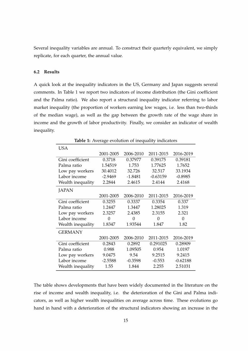
A quick look at the inequality indicators in the US, Germany and Japan suggests several

comments. In Table 1 we report two indicators of income distribution (the Gini coefficient

and the Palma ratio). We also report a structural inequality indicator referring to labor

market inequality (the proportion of workers earning low wages, i.e. less than two-thirds

of the median wage), as well as the gap between the growth rate of the wage share in

income and the growth of labor productivity. Finally, we consider an indicator of wealth

inequality.

Table 1: Average evolution of inequality indicators

USA2001-2005 2006-2010 2011-2015 2016-2019

Gini coefficient 0.3718 0.37977 0.39175 0.39181Palma ratio 1.54519 1.753 1.77625 1.7652Low pay workers 30.4012 32.726 32.517 33.1934Labor income -2.9469 -1.8481 -0.63159 -0.8985Wealth inequality 2.2844 2.4615 2.4144 2.4168

JAPAN2001-2005 2006-2010 2011-2015 2016-2019

Gini coefficient 0.3255 0.3337 0.3354 0.337Palma ratio 1.2447 1.3447 1.28025 1.319Low pay workers 2.3257 2.4385 2.3155 2.321Labor income 0 0 0 0Wealth inequality 1.8347 1.93544 1.847 1.82

GERMANY2001-2005 2006-2010 2011-2015 2016-2019

Gini coefficient 0.2843 0.2892 0.291025 0.28909Palma ratio 0.988 1.09505 0.954 1.0197Low pay workers 9.0475 9.54 9.2515 9.2415Labor income -2.5588 -0.3598 -0.553 -0.62188Wealth inequality 1.55 1.844 2.255 2.51031

The table shows developments that have been widely documented in the literature on the

rise of income and wealth inequality, i.e. the deterioration of the Gini and Palma indi-

cators, as well as higher wealth inequalities on average across time. These evolutions go

hand in hand with a deterioration of the structural indicators showing an increase in the

15

proportion of poorly paid workers and a change in the share of wages lower than that of

productivity. The literature has highlighted a multiplicity of causes for this phenomenon in

the industrialized countries. For instance, globalization and the generalization of outsourc-

ing and offshoring practices have led to an atomization of labor markets and an increase

in precarious work (fixed-term contracts, temporary work, etc). This has been a factor of

wage compression. In addition, technological progress (automation, increasing role of dig-

ital technology) has accentuated the technological bias among the least qualified workers.

Inequalities in income and wealth have been fostered, by the increase in financial savings in

the wealthiest households and the increase in debt among the most financially constrained

households, by the greater gap between the rate of return on financial capital and the rate

of return on physical capital, a greater concentration of capital and a weakening of trade

union power, and the hyper-financialization of economies. Interested readers can refer to

the following recent papers in the abundant literature on the ramping inequalities in the

US (Bozio et al., 2020; Komlos, 2019; Saez and Zucman, 2020).

Table 4 shows our estimates and the figures in Appendix D show some graphs of the

natural interest rates, potential growth, GDP and output-gaps.

United States

We start with the results obtained for the United States. When inequalities are included

among the explanatory variables, potential growth become more volatile (see, Figure

1, blue curve). Omitting these variables thus leads to over- or underestimate potential

growth. Specifically, during time of strong recessions, here during the 2000-2002 dot-com

bubble bust and the 2008-2009 financial crisis, inequalities lead to more pronounced drops

in potential growth than usually admitted with the standard LW model. Comparing the

black and blue curves, we see that during the dot-com crisis the slowdown in potential

growth might have been under-estimated by more than 1%. The GR is likely to have led

potential growth to a decrease of up to −3%. In 2015 and 2016, the US experienced what

is sometimes referred to as an “invisible recession”with a sharp slowdown in business

investment caused by the conjunction of several factors (run-up of the dollar, drop in

international commodity prices, including oil, and slowing demand in the emerging

countries). In Figure 1, we see that the negative effects of these events on potential growth

might have been aggravated by the increasing inequalities, thereby leading to a trajectory

of potential growth below the LW path estimated without them.

16

The higher volatility of potential growth is transmitted to the natural interest rate as well

(see Figure 2). This can be seen by comparing the blue and black curves. A striking

-new- feature here is the existence of two regimes. We see one regime in which the

natural rate of interest is positive, around the years corresponding to the GR, and a second

regime with negative natural rates outside this period. One explanation is that, when

inequality variables are taken into account, the predominant channels linking the crisis to

the dynamics of the natural interest rate are neither linked to real variables (such as the rate

of return on capital), nor to monetary variables (quantitative easing policy). Indeed, if this

were the case, we would have observed a fall in the natural rate. Here, the main channel

through which inequalities may have influenced the natural rate is debt reimbursement by

the private sector. The crisis has led to a very high level of dis-saving by households and

firms. If we assume that the natural rate reflects the balance between aggregate savings

and investment, then massive deleveraging by the private sector, such as that observed

after the financial crisis, has raised the natural interest rate. This phenomenon is more

accentuated when inequalities are high.

Figure 3 shows that the financial crisis of 2008 resulted in a fall in the level of potential

GDP that was larger than the usual estimates (without inequality variables) suggest. A

comparison of output gaps in Figures 4a and 4b shows that, by not taking inequalities

into account, the depth of recessions (negative output gap) is often underestimated and

the extent of expansionary phases (positive output gaps) are overestimated. For the year

2009 we see a zero-output gap, which can be explained by the fact that the crisis has not

only caused a fall in aggregate demand but also, at the same time, it has led to a decline in

potential GDP.

Germany

Let us compare these results with those obtained for Germany. In this country, inequalities

rose sharply in the first half of the 2000s. The explanatory factors are multiple: the export-

led growth model prompted a small increase in wages, wealth inequality augmented more

than in any other euro area country, labour markets underwent a strong transformation

with the adoption of the Hartz reforms between 2006 and 2011, and the positive effects

of public redistribution policies 10 years after the German reunification halted. Figure 5

suggests that potential growth with inequalities was much lower than the standard esti-

mate. In particular, the blue curve indicates that the falls in potential growth may have

17

been underestimated during the 2009 financial crisis.

The two curves (with and without the inequalities) are, nonetheless, closer from 2013 on-

ward. One explanation can be that several factors have contributed to erasing the effects of

inequalities. There was a change in wage policies, which, in a context of sustained growth,

has led real wages to grow faster than labour productivity. This mechanically produced

an increase in the wage share out of total income and stimulated aggregate demand. The

difference between the curves, before and after 2013, could therefore illustrate the positive

effect on potential growth of the end of wage moderation. The closer curves may also

illustrate the effects of the introduction of a minimum wage from 2015.

Figure 6 shows that the path of the natural rate, with inequality variables, resembles that

of potential growth rate. In contrast to the United States, a significant fall in the rate can

be observed corresponding to the years of the GR. Figure 7 shows that inequalities can

also imply a drop in the level of potential GDP per-capita, thereby suggesting that the

estimated output-gaps in Germany may have been very much overestimated compared to

what they were.

Japan

Japan is an atypical case compared to the other two countries. Income and wealth

inequalities are as high as in the other industrialized countries and the country has a large

number of poor people (16% of the population lives below the poverty line). Strangely, this

has little effect on the estimates of potential GDP and output-gaps (see Figures 8, 9 and 10).

Inequalities, however, affect potential growth and the natural interest rate. Inequality tends

to undermine potential growth when the latter is positive (in Figure 8, when g∗ is positive,

the black curve is very often above the blue one). However, during strong recessions, the

curves have the reverse positions, which suggests that households with the lowest incomes

and wealth are not necessarily those who suffer the most from recessions.

As in the US case, the estimated natural interest rate with inequality variables is more

volatile than the standard natural interest rate. The V-shaped curve suggest that both

natural rates have been influenced by monetary policy. First, since the beginning of the QE

policy in March 2001, the natural rate has remained negative most of the time. We see the

large trough corresponding to the implementation of the CME (Comprehensive Monetary

18

Easing) policy. Such a policy consisted in buying sovereign and risky corporate bonds

from the private sector, and at the same time engaging into a forward guidance policy to

anchor inflation expectations. Such a policy caused the natural rate to plunge due to the

abundance of liquidity in the markets. It can be noticed that, although negative, the natural

interest rate evolves along a positive trend since 2016, the year of the implementation of

the QQE policy (Quantitative and Qualitative Easing) aiming at redressing the right-end of

the yield curve to raise the level of long-term interest rates.

Comparing the estimation with and without inequality variables

Table 4 shows our estimates. The numbers in bold are the coefficients that are statistically

significant at 5% level of significance. signif is the significance level. The columns labelled

(1) correspond to estimates with inequality variables and those labelled (2) show estimates

without inequality variables.

For the United States, we see that GDP persistence, usually captured by the LW model,

disappears when inequality variables are introduced. The output gap variable is no longer

significant in the AS equation. Wealth inequality and inequalities captured by income

dispersion contribute to a decrease in potential GDP and thus to a wider output-gap

(which is indicated by a positive coefficient of the Palma ratio and wealth variables).

Moreover, when the number of low-wage earners rises, this has deflationary pressure. The

coefficient of the output-gap in the AS curve becomes insignificant in the equation with the

inequality variables, which can be explained as follows: inequality reduces the likelihood

of a strong effect of an expansion on employment, thereby reducing the upward pressure

on wages and hence on prices.

The estimates for Japan contrast with those obtained for the United States. The inequalities

measured by the Palma ratio and those related to wealth favor the appearance of recessions

(negative signs of the Palma ratio and Wealth coefficients). The aggregate supply curve is

vertical (the coefficient of the output gap, which is very high, becomes significant when

inequality variables are introduced into the AS equation). This is consistent with the

observation of persistent disinflation - or even deflation - in Japan. Low wages contribute

twice as much to disinflation there than in the US. Unlike the US, the introduction of

inequality variables in the model has little effect on the estimated coefficients for Japan.

19

For the German case, some results are identical to those of Japan. Specifically, inequalities

linked to Wealth and Palma ratio are likely to increase the risk of recessions (we find

negative and significant coefficients for these variables). On the other hand, the sign of the

low paid workers variable is positive, which is a consequence of the German export-led

growth model: wage compression has been an element of competitiveness of the German

economy on world markets. Unlike the other two countries, we find a down-sloping

aggregate supply curve. There are several explanations. The first is the existence of

important economies of scale: as output rises, costs per unit decrease. Another explanation

is that lower prices mean higher profits for the economy.

Concerning the variable "gender gap" it turns out to be significant in the three cases, al-

though the sign is different: positive for the United States and Japan and negative for Ger-

many. A potential explanation would be based on the models relating fertility to growth,

with the following underlying mechanism. Assume that an economy’s capital per-worker

is more complementary to women’ labor than to men’s. An increase in the gender gap (in

the case of our variable, a higher percentage of men relative to women participating in the

labor market) reduces women’s relative wages (as share of total wages). This lowers the

opportunity cost of having children. An increase in fertility is thus accompanied by a lower

growth rate (because lower women’s labor supply means lower capital) and this exerts a

negative impact on the natural interest rate. If instead capital and women’ labor are sub-

stitutable, we have the opposite effect of an increase in the gender gap. If the explanation

holds, then the positive sign for the US and Japan and the negative sign for Germany would

capture the fact that, in Germany, capital per worker is more complementary to women -

compared to the other two countries.

In all regressions, the impact of the real interest rate gap on the output-gap seems to be

very weak. All the estimated output-gaps display persistent dynamics.

7 Implications for monetary policy rules

7.1 A simple analytical model

We now investigate whether taking inequality into account in the calculation of the natural

interest rate (which is a target for the short-term policy rate) and potential GDP changes

20

the stance of monetary policy relative to a situation where these considerations are omitted.

The idea that monetary policy has a role to play in combating inequalities is gaining

renewed interest in the economic debate, after having been supplanted by an approach

focused exclusively on controlling inflation and fighting unemployment though the issue

is an old one. For example, in the United States, the Community Reinvestment Act allows

the US Federal Reserve to adopt measures facilitating access to credit for the lowest income

households. The economic literature has highlighted different transmission channels. The

first effects occur through "inflation tax" on nominal cash holdings of the lowest-income

households, while at the same time rising prices increase the value of real assets held

by higher-income households. Indeed, the wealth of the former is more often held in

monetary form (cash deposits), whereas the latter more easily own real assets (for example,

housing or businesses). Other redistributive effects play through nominal interest rate

changes. Interest rate cuts have two effects. On the one hand, they lead to a redistribution

from savers or lenders to borrowers (with possible intergenerational transfers insofar

as savers are old and borrowers are young). On the other hand, they increase wealth

inequality, as the reduction in interest rates pushes up the prices of financial assets (thus

increasing the wealth of the richest agents). Finally, monetary policy, through its effect on

the business cycle, can change the distribution of income as a result of employment effects.

Lower interest rates stimulate growth and employment. The redistributive effects depend

on the position of workers in the wage and income distribution, and on the sensitivity of

the types of jobs - skilled and unskilled - to variations in aggregate demand.

To build intuition about the impact of inequality on the stance of monetary policy, it is

interesting to investigate whether the achievement of some targets on inequality variables

requires putting more weight on output and inflation gaps than in a standard framework.

Before looking at some empirical results, we build some intuition by considering a basic

conceptual framework.

We use a simple setup where a central bank bases its policy on an optimal interest rate rule.

Suppose that it has the following quadratic loss function in which, in addition to the usual

inflation-gap and output-gap, it is assigned the mandate of stabilizing inequalities. Define

w∗t the desired level of one the inequality variables defined in Equation 2 and consider the

following loss function:

Loss =−12

[yt

2 + θ πt2 + κ (rt − rt−1)

2 + ω (wt)2]

, (9)

21

where yt = yt − y∗t , πt = πt − π∗t , wt = wt − w∗t .

The introduction of inequality variables into the loss function of a central bank can be

motivated by the need to combat the risks of financial instability. Indeed, one of the

drivers of financial crises over the last decade in the industrialized countries has been the

explosion of private debt. Income inequalities have played an important role in the dy-

namics of household credit. Inequalities increased sharply in a context of impoverishment

of countries’ middle class. A preventive fight against financial crises therefore involves

redistributive policies aimed at reducing income inequalities. An alternative interpretation

is that, although the central bank is not directly responsible for policies to fight inequalities

(this is rather the responsibility of governments), it takes these policies into account when

setting its policy rate.

It is equivalent to choose the real interest rate rt or the nominal interest rate it as the policy

instrument since by definition it = rt + πt. (rt − rt−1) accounts for interest rate smoothing.

To describe the economy consider simpler forms of Equations (1) and (2):

yt = −µr(rt − r∗t ) + azzt + σyεyt , ε

yt ≈ N(0, 1). (10)

πt = bππt−1 + byyt + bwwt + σπεπ, επ ≈ N(0, 1). (11)

where wt and zt are one of the inequality variables that impact inflation and the output. We

omit the lags on the endogenous and exogenous variables to keep the presentation simple.

This does not change our arguments.

Our question is whether it is feasible to reach simultaneously yt = πt = wt = 0. Denoting

λ1 and λ2 the Lagrangian multipliers of the single period minimization program subject to

the constraints 10 and 11, we obtain the following first-order conditions:

∂L∂πt

= 0→ θ πt = λ1, (12)

∂L∂yt

= 0→ yt

by=

λ2

by− λ1, (13)

∂L∂rt

= 0→ κ (rt − rt−1) = λ2 µr, (14)

∂L∂wt

= 0→ −ω wt

bw= λ1. (15)

22

where λ1, λ2 measure the rate of change of the loss function as constraints (11) and (10) are

relaxed. We look at the effect of each of the constraints on the inflation-output trade-off.

Setting λ2 = 0, we obtain the following equalities

rr = rt−1, πt =−1by θ

yt, πt =−ω

bw θwt. (16)

Is inequality reduction compatible with the trade-off between inflation and output? Let us

recall from our estimation results the following sign of the coefficients of the variables Wt

(Table 2). +, 0,− indicate respectively a positive, non-significant or negative value of the

variable on inflation.

Table 2: Impact of inequality variables on inflationUSA Japan Germany

Gender-gap + + −Labor income 0 0 0

Low pay workers − − +

Suppose that inflation rate is below target (πt < 0). The central bank must cut the interest

rate to expand aggregate demand (according to the second equality in (16)). But it must

also ensure that inequalities are moving in the right direction to allow a decrease in

inflation. The third equality in (16) says that for inflation to increase wt should decrease

and so wt should diminish below its target.

Consider the example of low pay workers. A decrease in the proportion of workers with

low wages is inflationary in the United States and Japan. Therefore, in these countries, a

policy of wage increases when inflation is too "low" (below its target) is enough to raise

inflation and this development is compatible with the central bank’s policy of stimulating

demand (when the inflation rate is below the target the central bank lowers its policy rate).

In Germany, on the other hand, the sign of the coefficient of low pay workers in the inflation

equation is positive. This implies that a decrease in the number of low-paid workers has

deflationary effects, which prevents inflation from moving in the "right" direction to close

the inflation gap. Only an increase in the number of low-paid workers would be compatible

with the trade-off between inflation and unemployment. The monetary authorities thus

face a dilemma of increasing inflation at the cost of allowing inequalities to rise. If we

23

would consider the gender-gap, such a dilemma would be observed in the United States

and Japan.

This type of dilemma is explained by the fact that the introduction of inequalities in the

loss function "breaks" the divine coincidence in Blanchard’s sense. If ω = 0 (no inequalities

are taken into account), from the first-order conditions, we immediately have that at the

optimum, the interest rate is constant, and the inflation and output gaps are zero. The

divine coincidence describes the unique link between inflation and output: setting the

inflation rate at its target is sufficient to close the output gap. In the case where ω 6= 0, we

add a constraint and the relation is no longer unique.

Now, we consider the case where, instead of wt, one of the variables in the vector Zt enters

the loss function. Our interest focuses on the gap zt. Combining the first-order conditions

and setting λ1 = 0, we obtain the following conditions:

πt = 0, yt =κ

µr(rt − rt−1), yt =

−ω

az(zt). (17)

Unlike before, where at the optimum the interest rate was fixed (we had rt = rt−1), the

interest rate has now a variance that is not zero. The central bank changes its policy rate

to keep inflation at its target, and any difference in interest rates observed between two

periods allows maintaining an output gap compatible with a certain level of inequality.

Assume that µr < 0, ω > 0, and κ > 0. The sign of az measures the impact of inequalities

on the output-gap. Based on our estimations, the sign of the coefficients in the (AD) curve

are shown in Table 3.

Table 3: Impact of inequality variables on output-gapUSA Japan Germany

Gini index − + 0Palma ratio + − 0

Wealth inequality + − −

Suppose that ar is positive. When output falls below its potential, the interest rate must fall

to stimulate demand. This must be compatible with a reduction in inequality according to

the second and third equality of (17). Conversely, if ar is negative, the increase in output

resulting from the rate cut is only compatible with an increase in inequalities above their

target.

24

Considering the example where the loss function includes the variable w as an inequality

indicator, the first-order conditions of the constrained minimization program yield two

reaction functions (two interest rate rules):

rt = rt−1 +(µr

κ

)yt +

(µr by θ

κ

)πt. (18)

and

rt = rt−1 +(µr

κ

)yt −

(µr by ω

κ bw

)wt. (19)

The two rules coincide if there are some economic mechanisms that guarantee the existence

of a particular relationship between the inflation gap and the inequality gap:

πt =( −ω

θ bw

)wt. (20)

In this case, it is equivalent to targeting inflation or inequalities, and the interest rate rule is

described by Equation (18). But if the constraint described by Equation (20) is not satisfied,

then the central bank must take its decision based on a combination of the two rules (18)

and (19). In this case, the weight assigned to the output target is identical to that of a rule

without the inequality variables, but the weight assigned to the inflation target is lower.

Indeed, an example of a composite rule is a linear combination leading to

ξ rt (given by 18) + (1− ξ) rt (given by 19), ξ ∈ (0, 1). (21)

i.e.

rt = rt−1 +(µr

κ

)yt + ξ

(µr by θ

κ

)πt + (1− ξ)

(−µr by ω

κ bw

)wt. (22)

The same type of arguments applies if instead of wt, one of the inequality variables zt that

influence aggregate demand is considered in the loss function.

The first order conditions lead to the following two equations:

rt = rt−1 +(µr

κ

)yt +

(µr by θ

κ

)πt, (23)

and

rt = rt−1 −(ω µr

κ az

)zt +

(µr by θ

κ

)πt. (24)

25

The two rules coincide if

yt =(− ω

az

)zt. (25)

If the constraint (25) is satisfied, it is equivalent to stabilize output and inequalities. (18)

and (23) are similar. If not, then the central bank must adopt a mixture of both rules:

rt = rt−1 +(µr by θ

κ

)πt + ξ

(µr

κ

)yt + (1− ξ)

(−ω µr

κ az

)zt. (26)

In this case, the coefficient of the output gap changes compared to a situation without

inequalities in the loss function. If we introduce the two types of inequality into the loss

function, both coefficients of the output gap and the inflation gap would change.

Our conclusion is as follows. When inequality variables are introduced into the central

bank’s objective function, this has two possible effects for the interest rate rules. The first is

a case of divine coincidence: by simply targeting inflation and the output gap, the central

bank also stabilizes inequalities. But this presupposes the verification of constraints linking

them. The second case is when the central bank has an instrument to achieve three different

objectives. This changes the sensitivity of the variation in interest rates to the output gap

and the inflation gap.

7.2 Econometric evidence

To "test" the conclusions of the previous section on real data, we estimate three reaction

functions supposed to describe the monetary policy of the US, Germany and Japan.

The first equation is the dynamic form of a standard interest rate rule where the gap be-

tween the short-term interest rate and its target depends on the inflation growth rate gaps.

The interest rate target corresponds to the natural interest rate estimated in the previous

sections (without inequality variables in AS and AD equations) and the growth target corre-

sponds to the potential growth rate estimated from the same model without the inequality

variables:

[1− β(L)

](rn

t − r∗t − π∗t)= c + αg(L)

(gt−1 − g∗t−1

)+ απ(L)

(πt−1 − π∗t−1

)+ ε1

t , (27)

where

rnt : nominal short-term rate = real shadow rate+core inflation;

26

r∗t + π∗t : nominal natural rate of interest;

r∗t : natural rate of interest estimated in the last section; π∗t : inflation target = 2%;

gt − g∗t : growth gap = observed growth minus potential growth estimated in the last sec-

tion;

πt: inflation rate;

εt: residual term;

and α(L) and β(L) are lag polynomials.

The second equation is similar to Equation (27) but r∗t and g∗t are the natural interest rate

and potential growth estimated in the last section when inequality variables are considered

in the AS and AD equations:

[1− β(L)

](rn

t − r∗t,ineq − π∗t)= c + αg(L)

(gt−1 − g∗t−1,ineq

)+ απ(L)

(πt−1 − π∗t−1

)+ ε2

t , (28)

In the third regression, we add the inequality variables that are in AD and AS as explana-

tory variables along with the inflation and growth gaps:

[1− β(L)

](rn

t − r∗t,ineq − π∗t)= c + αg(L)

(gt−1 − g∗t−1,ineq

)+ απ(L)

(πt−1 − π∗t−1

)+

Θ(L)Wt + Ω(L)Ztt + ε3t ,

(29)

The symbols in bold indicate vectors. The components of Θ(L) and Ω(L) are lag

polynomials.

Equations (27) to (29) are estimated using ARDL estimator (autoregressive distributed lag)

with a maximum of 2 lags.

Tables 5 to 10 present the estimation results for the three countries. We distinguish two

periods, before and after 2008, taking into account the changes in monetary policy regime.

We investigate the reaction function of the central banks’ interest rate had they followed

a policy rate setting rule involving stabilization objectives of the inequality variables at

target values.

When inequality variables are considered into the interest rate equation, at least one has

27

a significant coefficient. This is evidence of the absence of "divine coincidence". When

central banks calculate their natural interest rate target and potential growth (r∗ and g∗)

from a model that takes into account the macroeconomic consequences of inequality,

targeting and stabilizing inflation and/or the output gap alone is not enough to stabilize

the inequality variables around their target. When inequality variables are not included in

the regressions (where r∗ and g∗ are calculated taking into account the Z and W variables),

the parameters change, which suggests the presence of omission bias.

What would have been the reaction function of central banks if they had followed a policy

rate setting rule that took into account the stabilization objectives of inequality variables at

target values? To answer we compute for each sub-period the first and the third regressions.

In the United States, before 2008, the reaction function without the inequality variables

shows a counter cyclical reaction to inflation and growth gaps. Indeed, the significant

coefficients are positive (i.e. 2.17 for inflation and 0.9 = 0.26− 0.16 for growth). Taking

into account inequality objectives would have led the Fed to change the stance of monetary

policy, by conducting a pro-cyclical policy with regards to growth (the coefficient of the

growth gap turns to negative, i.e. -0.24) and by having a less stringent counter-cyclical

policy with respect to inflation (the coefficient decreases to 0.16=4.02-3.86).

The post-2008 period corresponds to the implementation of unconventional monetary

policies. The reaction function without inequality variables shows that the monetary policy

stance does not depend on the growth gap and is positively correlated with the inflation

gap (the coefficient is positive, i.e. 0.36 = 1.63-1.27). The period of significant interest

rate decline coincided with a strong period of disinflation. Taking account of inequality

variables would have made monetary policy stance weakly pro-cyclical with respect to

growth (the coefficient equals -0.06=-0.27+0.19) and weakly counter-cyclical with respect to

inflation (the coefficient is 0.75=1.55+1.61-2.41).

In the case of Japan, before 2008, monetary policy, without inequality variables, was

strongly counter-cyclical in a context of disinflation, when the Bank of Japan started

(before the other central banks) unconventional policies in the hope of bringing up prices.

The addition of inequality objectives would have led to a strengthening of this policy

(with a positive coefficient for the inflation gap rising from 2.54 to 4.79) and a pro-cyclical

28

policy favoring growth (negative coefficient equal to -0.18). For the post-2008 period, the

monetary policy stance depends on the growth rate gap in a pro-cyclical manner, when

inequality variables are not included in the reaction function. Introducing these variables

in the equation changes the sign of the coefficients of inflation and growth gaps: they

respectively turn from zero -insignificant - to a negative value for the former and from a

negative (-0.64) to a positive value (i.e -2.03=1.02-3.05) for the latter. Thus, taking inequality

into account would have led to the promotion of growth above potential growth - and

thus to the adoption of a policy leading to lower interest rates - while controlling infla-

tionary pressures in order to avoid its potential negative effects on the increase in inequality.

The results for Germany in the pre-2008 period are similar to those obtained for the

United States. Indeed, without inequalities, the interest rate policy is counter-cyclical,

both in terms of inflation control and growth (the coefficients are significantly positive).

Then, incorporating inequalities would have made it pro-cyclical, since the coefficients of

both gaps become significantly negative. After 2008, the highly expansive unconventional

monetary policy is de facto pro-cyclical and the effect on the stance of monetary policy

appears on the coefficient of inflation, which is negative in the first regression. The policy

would have been pro-cyclical if inequality targets had been added to the policy rule.

The results obtained for the three countries suggest that taking inequality into account in

central banks’ monetary policy would have changed the stance of monetary policy. Ac-

cording to the standard economic analysis, a surge in inflation or an economic recovery

above potential growth should push the policy rate up (because the positive sign of the

coefficients is a necessary condition for the stability of the macroeconomic equilibrium in

the AS-AD model). We show that taking inequality into account may lead to a change in

this orientation with, on the contrary, a policy that encourages inflationary recoveries (this

may help, for example, to reduce the real debt burden for the poorest households) and to

stimulate growth recoveries (given the beneficial effects on income, employment, etc).

8 Conclusions

In this paper, we have attempted to provide new estimates of the natural interest rates

and potential growth taking into account the role of inequality variables in both aggregate

demand and aggregate supply. Our results suggest that the omission of inequality issues

29

may generate biases in economic interpretation, since we have seen that such variables

can modify drastically the paths of interest rates and growth at their neutral levels. Inter-

estingly, for the United States, our findings are in accordance with the view that natural

rates are driven by the financial cycle, which could explain a negative correlation between

potential growth and neutral interest rates in both times of recessions and expansions.

Therefore, growing inequality may constitute a drawback for the recovery of the economy.

Another interesting finding concerns Japan, where inequality does not seem to affect that

much the estimates of output-gaps and potential GDP.

Since the natural rate of interest is usually presented as a possible target for the policy rate

of central banks, we studied the effects of our estimates for the reaction functions of the

monetary authorities, assuming that they are derived from loss functions that include the

objectives of monetary policy. We find two results to be important. First, that the presence

of inequality variables calls into question the idea that all possible policy objectives are

"subordinated" to the inflation objective. This was true in an economy where only the

inflation-growth trade-off is considered. In this case, stabilizing inflation is enough to

stabilize growth. The introduction of inequality targets breaks this automatic link. This

forces central banks to make "concessions" on their usual objectives. Thus, a second

important result is that the monetary policy aiming at stabilizing inflation and growth can

become pro-cyclical. When inequality is high, rather than curbing a recovery for fear that

it will eventually lead to inflationary pressures, it may be preferable to accompany it (by

cutting rates rather than raising them). The exercise in the previous section can be applied

to a situation where the central banker continues to target inflation and employment, but

incorporates fiscal policy objectives into its loss function. In this case, the loss function we

introduced could be applied to study the effects of a policy mix around inequality. Making

concessions on inflation and growth is a way for the monetary authorities to accompany

the fiscal authorities in the fight against inequality. Another possible interpretation is that

central banks can set their natural interest rate and potential growth targets with a view

to directing the financing of the economy towards activities that contribute to reducing

inequality.

Despite the interesting results, our work deserves some caution, as our estimation of the

natural rate contains the usual caveats of the LW models. A pitfall is the sensitivity of the

estimates to the selection of the starting values for the parameters, which sometimes makes

30

the estimates difficult to interpret.

31

References

Acemoglu, D., Johnson, S., and Robinson, J. (2004). Institutions as the Fundamental Cause of Long-Run Growth.

NBER Working Paper Series, 284.

Aiyagari, S. R. (1994). Uninsured Idiosyncratic Risk and Aggregate Saving. The Quarterly Journal of Economics,

109(3):659–684.

Alesina, A. and Perotti, R. (1996). Income distribution, political instability, and investment. European Economic

Review, 40(I 996):1203–1228.

Amaral, P. (2017). Monetary Policy and Inequality. Economic Commentary. Federal Reserve Bank of Cleveland.

Baldwin, R. (2019). The globotics upheavel: globalization, robotics and the future of work, volume 98. Oxford

University Press, New York, NY, USA.

Baldwin, R. (2020). The COVID-19 upheaval scenario : Inequality and pandemic make an explosive mix. VOX

CEPR Policy Portal, pages 1–5.

Baldwin, R. and Weder di Mauro, B. (2020). Economics in the Time of COVID-19. CEPR, London.

Bartscher, A. K., Kuhn, M., and Schularick, M. (2020). The college wealth divide: Education and inequality in

America, 1956-2016. Federal Reserve Bank of St. Louis Review, 102(1):19–49.

Benigno, G. and Fornaro, L. (2018). Stagnation traps. Review of Economic Studies, 85(3):1425–1470.

Bernanke, B. B. I. (2015). Why are interest rates so low , part 2 : Secular stagnation.

Bhaumik, S. (2011). Productivity and the Economic Cycle. BIS Economics Paper, 12.

Blanchard, O. J. (1985). Debt, Deficits, and Finite Horizons. Journal of Political Economy, 93(2):223–247.

Bozio, A., Garbinti, B., Goupille-Lebret, J., Guillot, M., and Piketty, T. (2020). Predistribution vs. Redistribution:

Evidence from France and the U.S. CEPR Discussion Paper Series, 15415.

Brynjolfsson, E. and McAfee, A. (2014). Second Machine Age: Work, Progress, and Prosperity in a Time of Brilliant

Technologies. Norton & Company.

Calvert Jump, R. (2018). IInequality and Aggregate Demand in the IS-LM and IS-MP Models. Bulletin of

Economic Research, 70(3):269–276.

Cuberes, D. and Teignier, M. (2012). Gender Gaps in the Labor Market and Aggregate Productivity. Sheffield

Economic Research Paper Series, 2012017.

Cynthia Fan Dora Xia, J. W. (2016). Measuring the Macroeconomic Impact of Monetary Policy at the Zero

Lower Bound. Journal of Money, Credit, and Banking, 48(2-3):253–291.

Eggertsson, G. B., Mehrotra, N. R., and Robbins, J. A. (2019). A model of secular stagnation: Theory and

quantitative evaluation. American Economic Journal: Macroeconomics, 11(1):1–48.

32

Engen, E. M. and Gruber, J. (2001). Unemployment insurance and precautionary saving. Journal of Monetary

Economics, 47(3):545–579.

Faggio, G., Salvanes, K., and Reenen, J. V. (2007). The Evolution of Inequality in Productivity and Wages: Panel

Data Evidence. NBER Working Paper Series, 13351.

Fornaro, L. and Wolf, M. (2020). COVID-19 Coronavirus and Macroeconomic Policy. CEPR Discussion Paper

Series, 20(14529).

Furman, J. and Orszag, P. (2018). Slower Productivity and Higher Inequality: Are They Related? Peterson

Institute for International Economics WP, 4.

García-Penalosa, C. (2007). Growth and income distribution in an integrated Europe : Does EMU make a

difference? Conference Paper. Forth Annual DG ECFIN Research Conference, (October):1–39.

Gertler, M. (1999). Government debt and social security in a life-cycle economy. Carnegie-Rochester Conference

Series on Public Policy, 50:61–110.

Gordon, R. J. (2012). Is U.S. economic growth over? faltering innovation confronts the six headwinds. NBER

Working Paper Series, 12.

Gordon, R. J. (2016). The Rise and Fall of American Growth: The U.S. Standard of Living since the Civil War. Princeton

University Press, Princeton, New Jersey.

Hansen, A. H. (1939). Economic Progress and Declining Population Growth. American Economic Review, 98(5):i–

v.

Holston, K., Laubach, T., and Williams, J. C. (2017). Measuring the natural rate of interest: International trends

and determinants. Journal of International Economics, 108:S59–S75.

Kaplan, G., Violante, G. L., and Weidner, J. (2014). The wealthy hand-to-mouth. Brookings Papers on Economic

Activity, Spring 201:139–153.

Komlos, J. (2019). Growth of Income and Welfare in the U.S., 1979-2011. Journal of Income Distribution, 28(1):1–19.

Krippner, L. (2015). A comment on Wu and Xia (2015), and the case for two-factor Shadow Short Rates.

Australian National University CAMA Working Paper, 48.

Krugman, P. (2014). Currency Regimes, Capital Flows, and Crises. IMF Economic Review, 62(4):470–493.

Laubach, T. and Williams, J. C. (2003). Measuring the Natural Rate of Interest. The Review of Economics and

Statistics, 85(November):1063–1070.

OECD (2018). Decoupling of Wages from Productivity: What Implications for Public Policies? In OECD

Economic Outlook, chapter 2, pages 51–65. OECD, Paris.

Oh, H. and Reis, R. (2012). Targeted transfers and the fiscal response to the great recession. Journal of Monetary

Economics, 59(SUPPL.):S50–S64.

33

Rachel, L. and Smith, T. D. (2015). Secular drivers of the global real interest rate. Bank of England Staff Working

Paper, (571).

Rodrik, D. (1999). Where did all the Growth Go? External shocks, social conflict, and growth collapses. Journal

of Economic Growth, 4(4):385–412.

Rogoff, K. (2015). Debt Supercycle, Not Secular Stagnation. VOX CEPR Policy Portal, pages 1–5.

Saez, E. and Zucman, G. (2020). The rise of income and wealth inequality in America: Evidence from distribu-

tional macroeconomic accounts. Journal of Economic Perspectives, 34(4):3–26.

Stiglitz, J. E. (2012). The Price of Inequality: How Today’s Divided Society Engangers Our Future. W. W. Norton,

New York.

Summers, L. (2013). Why Stagnation Might Prove to Be the New Normal.

Taylor, J. B. (2016). Slow economic growth as a phase in a policy performance cycle. Journal of Policy Modeling,

38(4):649–655.

Wu, J. C. and Zhang, J. (2019). A shadow rate New Keynesian model. Journal of Economic Dynamics and Control,

107.

34

Tabl

e4:

Coe

ffici

ents

esti

mat

es

Uni

ted

Stat

esJa

pan

Ger

man

y

(1)

(2)

(1)

(2)

(1)

(2)

Var

iabl

esC

oeff

Sign

ifC

oeff

Sign

ifC

oeff

Sign

ifC

oeff

Sign

ifC

oeff

Sign

ifC

oeff

Sign

ifO

utpu

tga

p(-

1)0.

070.

781.

640.

001.

070.

001.

360.

001.

100.

000.

980.

00O

utpu

tga

p(-

2)0.

230.

32-0

.68

0.00

-0.4

70.

00-0

.67

0.00

-0.1

00.

72-0

.10

0.20

Inte

rest

rate

gap

0.00

0.06

0.00

0.09

0.00

0.02

0.00

0.20

0.00

0.36

0.00

0.01

Con

stan

t(A

D)

-0.3

30.

000.

000.

660.

100.

000.

000.

850.

090.

030.

000.

06O

utpu

tga

p(A

S)17

.57

0.12

8.04

0.00

268.

580.

0130

5.05

0.24

-2.1

60.

05-6

.02

0.03

Infla

tion

(-1)

0.90

0.00

0.82

0.00

-0.9

30.

00-0

.89

0.00

0.77

0.00

0.86

0.00

Oil

infla

tion

0.01

0.13

0.01

0.34

-0.1

20.

00-0

.14

0.00

0.00

0.50

0.00

0.59

Impo

rted

infla

tion

0.19

0.00

0.13

0.02

0.47

0.00

0.40

0.00

0.13

0.13

0.21

0.00

Var

ianc

e(A

D)

0.00

1.00

0.00

0.03

0.00

1.00

0.00

0.31

0.00

1.00

0.00

1.00

Var

ianc

e(A

S)0.

170.

000.

170.

00-0

.06

0.00

0.00

1.00

0.21

0.00

0.23

0.00

Var

ianc

epo

tent

ialo

utpu

t0.

000.

000.

000.

000.

010.

000.

000.

000.

010.

000.

010.

00

Var

ianc

eof

gov

erva

rian

ceof

outp

ut0.

360.

020.

180.

020.

260.

0010

71.2

20.

000.

760.

050.

660.

15

Var

ianc

eof

Zov

erva

rian

ceof

outp

ut19

2.12

0.22

0.00

1.00

-8.7

50.

00-0

.53

0.42

38.0

10.

420.

000.

00

C-8

49.2

30.

3345

0.22

0.42

-950

.63

0.00

2.89

0.00

228.

900.

4065

.09

0.63

Gin

i-0

.39

0.04

0.11

0.01

-0.0

60.

74Pa

lma

0.09

0.00

-0.0

30.

030.

040.

23W

ealt

h0.

010.

00-0

.04

0.00

-0.0

10.

00G

ende

r5.

390.

056.

700.

00-3

.80

0.01

Wag

es0.

000.

99-0

.01

0.38

0.00

0.90

Low

paid

-2.9

20.

05-4

.65

0.00

3.07

0.01

Not

e:C

oeffi

cien

tsin

bold

deno

tesi

gnifi

canc

e.T

heco

lum

nsla

belle

d(1)

and(2)

stan

dfo

rin

clud

ing

and

not

incl

udin

g,re

spec

tive

ly,i

nequ

alit

yva

riab

les.

35

Table 5: Monetary policy rule : USA - 2000-2008

USA 2001-2008 R* and y*without in-equality

R* and y* + in-equality

R* and y* + in-equality + exoge-nous variables

Gap variables Coefs. P-value Coefs. P-value Coefs. P-valueInterest rate(-1) 1.03∗∗∗ 0.0002 1.41∗∗∗ 0.0 0.83 0.006Interest rate(-2) -0.35 0.12 -0.44 0.14 -0.36 0.13Growth −0.16∗ 0.08 -0.12 0.43 −0.24∗∗ 0.02Growth(-1) 0.25∗∗ 0.04 - - -0.12 0.35Growth(-2) - - - - - -Inflation -1.04 0.27 −2.13∗ 0.07 −3.86∗∗∗ 0.003Inflation(-1) 2.17∗∗ 0.04 1.82∗ 0.07 4.02∗∗ 0.02Inflation(-2) - - - - -1.01 0.49Intercept -0.93** 0.04 -0.14 0.59 -37.51 0.92

Ineq. variables Coefs. P-value Coefs. P-value Coefs. P-value

Gini - - - - -0.84 0.43Gini(-1) - - - - 2.03 0.22Gini(-2) - - - - -1.00 0.29Palma - - - - 1.0∗∗∗ 0.02Palma(-1) - - - - −0.9∗ 0.06Palma(-2) - - - - 0.53 0.20Wealth - - - - −0.22∗ 0.06Wealth(-1) - - - - - -Wealth(-2) - - - - - -Gender - - - - 4.13∗∗ 0.05Gender(-1) - - - - -2.61 0.27Gender(-2) - - - - 1.37 0.46Income - - - - -0.001 0.72Income(-1) - - - - -0.002 0.38Income(-2) - - - - 0.01∗∗∗ 0.0038Low paid - - - - 199.02∗∗ 0.05Low paid(-1) - - - - -87.67 0.28Low paid(-2) - - - - - -

R2 0.81 - 0.87 - 0.99 -F bound test 1.96∗ - 0.43∗ - 8.6∗ -

36

Table 6: Monetary policy rule : USA - 2009-2019

USA 2009-2019 R* and y*without in-equality

R* and y* + in-equality

R* and y* + in-equality + exoge-nous variables

Gap variables Coefs. P-value Coefs. P-value Coefs. P-valueInterest rate(-1) 1.13∗∗∗ 0.0 1.19∗∗∗ 0.0 0.63∗∗∗ 0.0Interest rate(-2) −0.27∗∗ 0.0 −0.24∗ 0.08 - -Growth 0.07 0.40 0.23∗∗ 0.03 0.19∗∗ 0.01Growth(-1) -0.13 0.12 -0.09 0.27Growth(-2) −0.27∗∗∗ 0.0001Inflation −1.27∗∗ 0.05 −1.45∗ 0.06 −2.41∗∗∗ 0.002Inflation(-1) 1.63∗∗ 0.02 1.83** 0.01 1.61* 0.08Inflation(-2) 1.55∗∗ 0.02Intercept -0.60** 0.05 0.01 0.95 −164.01∗∗ 0.03

Ineq. variables Coefs. P-value Coefs. P-value Coefs. P-valueGini - - - - 8.40*** 0.0Gini(-1) - - - - −4.11∗∗∗ 0.0018Gini(-2) - - - - -Palma - - - - −0.43∗∗ 0.02Palma(-1) - - - - - -Palma(-2) - - - - - -Wealth - - - - 0.01* 0.06Wealth(-1) - - - - - -Wealth(-2) - - - - - -Gender - - - - 2.22*** 0.0004Gender(-1) - - - - -1.66*** 0.002Gender(-2) - - - - - -Income - - - - 0.0006*** 0.0024Income(-1) - - - - 0.001*** 0.0Income(-2) - - - - 0.0003* 0.05Low paid - - - - 0.22 0.17Low paid(-1) - - - - -0.39** 0.03Low paid(-2) - - - - - -

R2 0.86 - 0.94 - 0.98 -F bound test 1.99* - 0.64* - 7.98* -

37

Table 7: Monetary policy rule: Germany - 2000-2008

GER 2001-2008 R* and y*without in-equality

R* and y* + in-equality

R* and y* + in-equality + exoge-nous variables

Gap variables Coefs. P-value Coefs. P-value Coefs. P-valueInterest rate(-1) 0.82*** 0.0 1.60*** 0.0 0.01 0.95Interest rate(-2) - - -0.68 0.0 0.43 0.15Growth 0.04 0.39 -0.02 0.66 -0.14** 0.02Growth(-1) 0.08* 0.07 0.25*** 0.0002 -0.04 0.56Growth(-2) 0.05 0.14 - - 0.06** 0.05Inflation 0.34* 0.08 0.13 0.59 -0.58* 0.09Inflation(-1) - - - - -0.94 0.09Inflation(-2) - - - - 0.53 0.31Intercept 0.94** 0.02 -0.46 0.23 940.93*** 0.002

Ineq. variables Coefs. P-value Coefs. P-value Coefs. P-valueGini - - - - 0.94 0.42Gini(-1) - - - - -0.97 0.53Gini(-2) - - - - -3.60 0.02Palma - - - - 0.36 0.17Palma(-1) - - - - -0.72* 0.07Palma(-2) - - - - 0.40** 0.05Wealth - - - - 0.08 0.73Wealth(-1) - - - - -0.19 0.50Wealth(-2) - - - - -0.62** 0.03Gender - - - - 0.11 0.92Gender(-1) - - - - 0.15 0.92Gender(-2) - - - - -1.44 0.32Income - - - - 0.05 0.13Income(-1) - - - - 0.07 0.13Income(-2) - - - - 0.13** 0.01Low paid - - - - 0.04 0.80Low paid(-1) - - - - -0.20 0.18Low paid(-2) - - - - - -

R2 0.90 - 0.95 - 0.99 -F bound test 1.99∗ - 2.23∗ - 17.8∗ -

38

Table 8: Monetary policy rule : Germany - 2009-2019

GER 2009-2019 R* and y*without in-equality

R* and y* + in-equality

R* and y* + in-equality + exoge-nous variables

Gap variables Coefs. P-value Coefs. P-value Coefs. P-valueInterest rate(-1) 1.21*** 0.0 1.24*** 0.0 0.83*** 0.0Interest rate(-2) -0.38*** 0.0027 -0.38 0.0011 -0.27** 0.05Growth 0.06 0.12 -0.04 0.30 -0.03 0.59Growth(-1) - - 0.12*** 0.007 0.05 0.28Growth(-2) - - - - - -Inflation -0.52 0.28 -0.22 0.65 0.13 0.80Inflation(-1) 1.53** 0.02 1.39** 0.02 0.81 0.18Inflation(-2) -2.11*** 0.0001 -2.12*** 0.0001 -1.22** 0.05Intercept -1.06*** 0.0039 -1.50 0.0002 -15.14 0.78

Ineq. variables Coefs. P-value Coefs. P-value Coefs. P-valueGini - - - - 6.61*** 0.0034Gini(-1) - - - - -6.92*** 0.001Gini(-2) - - - - - -Palma - - - - 0.005 0.98Palma(-1) - - - - -0.65* 0.08Palma(-2) - - - - 0.66** 0.01Wealth - - - - 0.04 0.69Wealth(-1) - - - - - -Wealth(-2) - - - - - -Gender - - - - 0.52 0.22Gender(-1) - - - - -1.46** 0.03Gender(-2) - - - - 0.86** 0.02Income - - - - 0.03 0.61Income(-1) - - - - 0.14** 0.02Income(-2) - - - - - -Low paid - - - - -0.13 0.12Low paid(-1) - - - - 0.30** 0.02Low paid(-2) - - - - -0.21*** 0.006

R2 0.95 - 0.97 - 0.98 -F bound test 5.26 - 10.02 - 6.46 -

39

Table 9: Monetary policy : Japan - 2000-2008

JAP 2001-2008 R* and y*without in-equality

R* and y* + in-equality

R* and y* + in-equality + exoge-nous variables

Gap variables Coefs. P-value Coefs. P-value Coefs. P-valueInterest rate(-1) 1.34*** 0.0 1.30*** 0.0 0.88** 0.01Interest rate(-2) -0.52** 0.02 -0.56 0.0017 -0.74*** 0.007Growth -0.73 0.28 -0.08 0.24 -0.02 0.77Growth(-1) - - -0.16* 0.047 -0.18*** 0.008Growth(-2) - - - - -0.07 0.25Inflation 2.54** 0.04 3.00* 0.07 -2.56 0.19Inflation(-1) -0.70 0.64 -2.98* 0.08 2.26 0.33Inflation(-2) -1.65 0.19 - - 4.79** 0.03Intercept 0.18 0.14 0.23 0.86 -732.38** 0.01

Ineq. variables Coefs. P-value Coefs. P-value Coefs. P-valueGini - - - - 10.36** 0.03Gini(-1) - - - - -3.68 0.24Gini(-2) - - - - - -Palma - - - - -0.90** 0.03Palma(-1) - - - - - -Palma(-2) - - - - - -Wealth - - - - -1.31** 0.02Wealth(-1) - - - - - -Wealth(-2) - - - - - -Gender - - - - -2.21 0.43Gender(-1) - - - - -6.09** 0.05Gender(-2) - - - - 12.43*** 0.001Income - - - - - -Income(-1) - - - - - -Income(-2) - - - - - -Low paid - - - - 1.82** 0.01Low paid(-1) - - - - -0.81 0.23Low paid(-2) - - - - 0.68 0.12

R2 0.87 - 0.84 - 0.97 -F bound test 1.43* - 4.16* - 7.36* -

40

Table 10: Monetary policy rule : Japan - 2009-2019

JAP 2009-2019 R* and y*without in-equality

R* and y* + in-equality

R* and y* + in-equality + exoge-nous variables

Gap variables Coefs. P-value Coefs. P-value Coefs. P-valueInterest rate(-1) 1.49*** 0.0 1.36*** 0.0 0.55*** 0.0036Interest rate(-2) -0.56*** 0.003 -0.47*** 0.008 -0.85*** 0.0Growth -0.07 0.84 -0.06 0.34 0.27*** 0.003Growth(-1) 0.42 0.26 -0.17** 0.013 0.17** 0.05Growth(-2) -0.64** 0.02 - - 0.08 0.17Inflation 0.25 0.32 1.49* 0.09 0.26 0.80Inflation(-1) - - -1.37 0.11 -3.05*** 0.0013Inflation(-2) - - - - 1.02* 0.10Intercept 0.60 0.13 -0.01 0.99 326.65*** 0.0035

Ineq. variables Coefs. P-value Coefs. P-value Coefs. P-valueGini - - - - -7.76 0.03Gini(-1) - - - - 9.35 0.14Gini(-2) - - - - -14.76*** 0.008Palma - - - - 0.87** 0.012Palma(-1) - - - - - -Palma(-2) - - - -Wealth - - - - -0.16 0.62Wealth(-1) - - - - - -Wealth(-2) - - - - - -Gender - - - - -1.33 0.41Gender(-1) - - - - 0.60 0.83Gender(-2) - - - - 2.14 0.22Income - - - - - -Income(-1) - - - - - -Income(-2) - - - - - -Low paid - - - - -0.20 0.19Low paid(-1) - - - - -0.37** 0.03Low paid(-2) - - - - -0.33* 0.08

R2 0.94 - 0.88 - 0.97 -F bound test 2.01 - 2.54 - 8.17* -

41

Appendix A Data sources and estimation results

Table 11: Sources and dataVariable Description Sourceyt Real GDP (per-capita). We take the loga-

rithm.OECD Database

rt Short-term real interest rate (nominal minusheadline inflation. We take the shadow nom-inal rate

OECD Database for inflation.CB of New Zealand for shadowrate

GINI Gini (disposable income post taxes Data andtransfers). Data are annual and transformedinto quarterly data Original data end in 2017.We replicate the 2017 values for 2018 and2019.

OECD income distributiondatabase

Income disparities Palma ratio: Share of top 10% over bottom40% (income distribution)

OECD income distributiondatabase

Wealth inequalities Total wealth share of top 10% of wealth / to-tal wealth share of bottom 60% of wealth

OECD Social and Welfare Statis-tics and for Households’ finan-cial and non-financial assets,OECD National Accounts Data

Family labour sta-tus

Ratio of perc. of children living in familywhere all adults work and perc. of childrenliving in family where only one adult works.Some data start in 2005. For the years 2000-2004, we replicate the data of 2005.

OECD Social and Welfare Statis-tics

πt Core inflation. Consumer prices, all foodsnon-food, non-energy

OECD Stat

Imported inflation G20 CPI all items. We compute core usingHP filter and we divide the results by coreinflation defined above.

OECD Stat

Oil prices Crude oil import prices. We compute core asthe HP filter trend calculated on the indexand we divide the result by domestic coreinflation.

OECD Data

Gender gap Labour force participation rate (ratio of menover women). Data are annual and convertedin quarterly data.

OECD Social and Welfare Wel-fare Statistics Statistics

Labour incomeshare growth rateminus productiv-ity growth rate

Labour income share ratios: Original dataare annual and converted to quarterly data.Productivity is measured by GDP per personemployed quarterly change).

OECD Data on unit labor cost

Low pay workers Share of workers earning less than two-thirdsof median earnings (full-time employees).Original data are annual and converted toquarterly data

OECD Wage levels.

42

Appendix B A simple model linking labour income share and prices in AS

equation

We propose a stylized model in which inequalities related to changes in the distribution of

income shares is shown to affect the dynamics of inflation in AS equation.

Nominal wage rate is set by employees, based on their expectations of future price level.

Consumer prices are a weighted average of producer and foreign prices:

(1 + Tdt )W

st = (1 + Tv

t )Pect, Pct = P1−φt

t (P∗t Et)φt , (A1)

where Wst is the nominal wage rate, Td

t and Tvt are tax rates on respectively wages (income

or payroll tax) and consumption goods (VAT). Pect is the expected level of consumer prices,

Et is the nominal exchange rate. φt is the share of foreign goods in the consumer’s basket

of consumption. Pt and P∗t are producer prices in the domestic and foreign countries.

Using a log-linearized form, the real wage rate depends on fiscal wedge and on the expected

level of consumer prices (small letter are log):

wst = (tv

t − tdt ) + pe

ct, pct − pt = φt + θt, θt = p∗t − pt + et. (A2)

θt is the real exchange rate defined as the ratio of foreign prices p∗t expressed in units of

domestic currency (et is the nominal exchange rate) to domestic prices pt. The weighting

coefficient φt is assumed to be variable over time. It can be considered as a proxy for the

degree of pass-through of foreign prices into domestic prices.

Firms produce Yt with labor (the employment level is Nt). The production function- in

logarithm - is written Yt = Nγtt , where γt denotes the share of wages out of national income

(wage share). For simplicity we assume that capital stock is fixed.

The first-order condition of profit maximization leads the firms to choose its optimal level

of employment. This choice implies

pt − pect = −lnγt + (tv

t − tdt ) + yt, (A3)

where yt is per-capita GDP (in logarithm). Inflation expectations are defined as a weighted

average of an anchor price and past consumer prices. In logarithms, we write:

pect = (1− λ) pct + λ Dpπ

π (L)pct, 0 < λ < 1. (A4)

43

Defining CPI inflation πct = ∆pct, total inflation πt = ∆pt, expected inflation πect = pe

ct, and

assuming that tax rates are constant, we obtain the following short-term aggregate supply

curve:

πct = πect + ∆ln(γt) + ∆yt + επ

t , (A5)

πect = (1− λ)πct + λDpπ

π (L)πct, 0 < γt < 1. (A6)

Equation (2) is obtained by assuming extrapolative expectations, λ = 1 in Equation (A6)

and by taking into account the cyclical nature of labor productivity dynamics (See Bhaumik

(2011) for empirical evidence in the industrialized countries). Further changes in the labour-

income share is equivalent to changes in the gap between the growth rate of wages and

productivity. Both have been shown to be linked to factors of inequalities (for instance,

gender gap) and international environment (here imported inflation and energy prices to

account for possible substitution between labour and factors of production that are energy-

based).

44

Appendix C State-space representation of the model

Xt = AXt−1 + ζt + Ftηt : state equation (B1)

Yt = µt + CTt Xt + GtVt : measurement equation (B2)

with the following definitions of the variables

Xt(7×1)

=

y∗ty∗t−1

y∗t−2

gt

gt−1

st

st−1

, A

(7×7)=

1 0 0 1 0 0 0

1 0 0 0 0 0 0

0 1 0 0 0 0 0

0 0 0 1 0 0 0

0 0 0 1 0 0 0

0 0 0 0 0 δg 0

0 0 0 0 0 1 0

, ζt(7×1)

=

0

0

0

0

0

g

0

0

,

ηt(3×1)

=

ε

y∗t

εgt

εst

, Ft(7×3)

=

σy∗ σg 0

0 0 0

0 0 0

0 σg 0

0 0 0

0 0 σs

0 0 0

, Yt

(2×1)=

yt

πt

,

45

µt(2×14)

=

AA 0 0

b1 0 BB

yt−1

yt−2

rt−3

rt−4

1

κt

Zt

Wt

, AAT

(8×1)=

a0y

a1y

ar 2

ar 2

a4

a1Gini

a1Palma

a1wealth

, BBT

(5×1)=

b1oil

b1imp

b1gender

b1wage

b1low

Vt(2×1)

=

εyt

επt

, Gt(2×2)

=

σy 0

0 σπ

, CT(7×2)

=

1 0

−a0y −b0

y

−a1y 0

− arc2 0

− arc2 0 0

− ar2 0

− ar2 0

[

ZT(1×3)

=

Ginit−1

Palmat−1

Wealtht−1

, κT(1×2)

=

poilt−1

pimpt−1

, W T(1×3)

=

Gendert−1

wagest−1

Lowt−1

.

46

Appendix D Figures

Figure 1: Time path of potential growth for the United States

Figure 2: Time path of the natural interest rate for the United States

Figure 3: Time path of potential GDP for the United States

47

(a) Time path of output gap for the United States

(b) Time path of output gap accounting for inequality. United StatesFigure 4: Output gap with and without inequality. United States.

48

Figure 5: Time path of potential growth for Germany

Figure 6: Time path of the natural interest rate for Germany

Figure 7: Time path of potential GDP for Germany

49

Figure 8: Time path of potential growth for Japan

Figure 9: Time path of the natural interest rate for Japan

Figure 10: Time path of potential GDP for Japan

50

(a) Time path of output gap for Japan

(b) Time path of output gap accounting for inequality. JapanFigure 11: Output gap with and without inequality. Japan.

51