FEDERAL RESERVE BANK OF SAN FRANCISCO

WORKING PAPER SERIES

Working Paper 2009-13 http://www.frbsf.org/publications/economics/papers/2009/wp09-13bk.pdf

The views in this paper are solely the responsibility of the authors and should not be interpreted as reflecting the views of the Federal Reserve Bank of San Francisco or the Board of Governors of the Federal Reserve System.

Do Central Bank Liquidity Facilities Affect Interbank Lending Rates?

Jens H. E. Christensen

Federal Reserve Bank of San Francisco

Jose A. Lopez Federal Reserve Bank of San Francisco

Glenn D. Rudebusch

Federal Reserve Bank of San Francisco

June 2009

Do Central Bank Liquidity Facilities

Affect Interbank Lending Rates?

Jens H. E. Christensen

Jose A. Lopez

Glenn D. Rudebusch

Federal Reserve Bank of San Francisco

101 Market Street

San Francisco, CA 94105

Abstract

In response to the global financial crisis that started in August 2007, central banks pro-

vided extraordinary amounts of liquidity to the financial system. To investigate the effect

of central bank liquidity facilities on term interbank lending rates, we estimate a six-factor

arbitrage-free model of U.S. Treasury yields, financial corporate bond yields, and term

interbank rates. This model can account for fluctuations in the term structure of credit

risk and liquidity risk. A significant shift in model estimates after the announcement of

the liquidity facilities suggests that these central bank actions did help lower the liquidity

premium in term interbank rates.

We thank conference participants at the Federal Reserve Bank of New York, the Federal Deposit InsuranceCorporation, the Board of Governors of the Federal Reserve System, the Bank of England, Koc University,and the Federal Reserve Bank of San Francisco—and especially, Pierre Collin-Dufresne and Simon Potter—forhelpful comments. The views in this paper are solely the responsibility of the authors and should not beinterpreted as reflecting the views of the Federal Reserve Bank of San Francisco or the Board of Governors ofthe Federal Reserve System.

Draft date: June 2, 2009.

1 Introduction

In early August 2007, amidst declining prices and credit ratings for U.S. mortgage-backed

securities and other forms of structured credit, international money markets came under

severe stress. Short-term funding rates in the interbank market rose sharply relative to yields

on comparable-maturity government securities. For example, the three-month U.S. dollar

London interbank offered rate (LIBOR) jumped from only 20 basis points higher than the

three-month U.S. Treasury yield during the first seven months of 2007 to over 110 basis points

higher during the final five months of the year. This enlarged spread was also remarkable for

persisting into 2008.

LIBOR rates are widely used as reference rates in financial instruments, including deriva-

tives contracts, variable-rate home mortgages, and corporate notes, so their unusually high

levels in 2007 and 2008 appeared likely to have widespread adverse financial and macroe-

conomic repercussions.1 To limit these adverse effects, central banks around the world es-

tablished an extraordinary set of lending facilities that were intended to increase financial

market liquidity and ease strains in term interbank funding markets, especially at maturities

of a few months or more. Monetary policy operations typically focus on an overnight or very

short-term interbank lending rate. However, on December 12, 2007, the Bank of Canada, the

Bank of England, the European Central Bank (ECB), the Federal Reserve, and the Swiss

National Bank jointly announced a set of measures designed to address elevated pressures

in term funding markets. These measures included foreign exchange swap lines established

between the Federal Reserve and the ECB and the Swiss National Bank to provide U.S. dol-

lar funding in Europe. The Federal Reserve also announced a new Term Auction Facility, or

TAF, to provide depository institutions with a source of term funding. The TAF term loans

were secured with various forms of collateral and distributed through an auction.

The TAF and similar term lending facilities by other central banks were not monetary

policy actions as traditionally defined.2 Instead, these central bank actions were meant to

improve the distribution of reserves and liquidity by targeting a narrow market-specific fund-

ing problem. The press release introducing the TAF described its purpose in this way: “By

allowing the Federal Reserve to inject term funds through a broader range of counterparties

and against a broader range of collateral than open market operations, this facility could help1As a convenient redundancy, we follow the literature in referring to “LIBOR rates.”2The Federal Reserve, in its normal operations, tries to hit a daily target for the federal funds rate, which

is the overnight interest rate for interbank lending of bank reserves. The central bank liquidity facilities werenot intended to alter the current level or the expected future path for the funds rate or the overall level ofbank reserves (i.e., the term lending was sterilized by sales of Treasury securities).

1

promote the efficient dissemination of liquidity when the unsecured interbank markets are

under stress.” (Federal Reserve Board, December 12, 2007).

This paper assesses the effect of the establishment of these extraordinary central bank

liquidity facilities on the interbank lending market and, in particular, on term LIBOR spreads

over Treasury yields. In theory, the provision of central bank liquidity could lower the liquidity

premium on interbank debt through a variety of channels. On the supply side, banks that

have a greater assurance of meeting their own unforseen liquidity needs over time should

be more willing to extend term loans to other banks. In addition, creditors should also be

more willing to provide funding to banks that have easy and dependable access to funds,

since there is a greater reassurance of timely repayment. On the demand side, with a central

bank liquidity backstop, banks should be less inclined to borrow from other banks to satisfy

any precautionary demand for liquid funds because their future idiosyncratic demands for

liquidity over time can be met via the backstop. However, assessing the relative importance

of these channels is difficult. Furthermore, judging the efficacy of central bank liquidity

facilities in lowering the liquidity premium is complicated because LIBOR rates, which are

for unsecured bank deposits, also include a credit risk premium for the possibility that the

borrowing bank may default. The elevated LIBOR spreads during the financial crisis likely

reflected both higher credit risk and liquidity premiums, so any assessment of the effect of

the recent extraordinary central bank liquidity provision must also control for fluctuations in

bank credit risk.

To analyze the effectiveness of the central bank liquidity facilities in reducing interbank

lending pressures, we use a multifactor arbitrage-free (AF) representation of the term struc-

ture of interest rates and bank credit risk. Specifically, we estimate an affine arbitrage-free

term structure representation of U.S. Treasury yields, the yields on bonds issued by finan-

cial institutions, and term LIBOR rates using weekly data from 1995 to midyear 2008. For

tractability, the model uses the arbitrage-free Nelson-Siegel (AFNS) structure. Christensen,

Diebold, and Rudebusch (CDR, 2007) show that a three-factor AFNS model fits and forecasts

the Treasury yield curve very well and avoids many of the estimation difficulties encountered

with unrestricted AF latent factor models. In this paper, we incorporate three additional fac-

tors: two factors that capture bank debt risk dynamics, as in Christensen and Lopez (2008),

and a third factor specific to LIBOR rates. The resulting six-factor representation provides

arbitrage-free joint pricing of Treasury yields, financial corporate bond yields, and LIBOR

rates. This structure allows us to decompose movements in LIBOR rates into changes in bank

debt risk premiums and changes in a factor specific to the interbank market that includes

2

a liquidity premium. We can also conduct hypothesis testing and counterfactual analysis

related to the introduction of the central bank liquidity facilities.

Our results support the view that the central bank liquidity facilities established in Decem-

ber 2007 helped lower LIBOR rates. Specifically, the parameters governing the term LIBOR

factor within the model are shown to change after the introduction of the liquidity facilities.

The hypothesis of constant parameters is overwhelmingly rejected, suggesting that the be-

havior of this factor, and thus of the LIBOR market, was directly affected by the introduction

of central bank liquidity facilities. To quantify this effect, we use the model to construct a

counterfactual path for the 3-month LIBOR rate by assuming that the LIBOR-specific factor

remained constant at its historical average after the introduction of the liquidity facilities.

Our analysis suggests that the counterfactual 3-month LIBOR rate averaged significantly

higher—on the order of 70 basis points higher—than the observed rate from December 2007

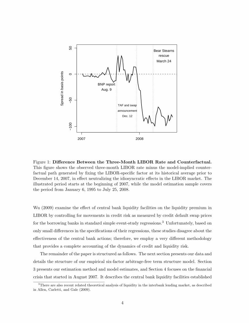
through the middle of 2008. Figure 1 shows the difference between the observed three-month

LIBOR rate and our model-implied counterfactual path for that rate during this period. From

the start of the financial crisis—which was triggered by an August 9, 2007, announcement by

the French bank BNP Paribas—until the TAF and swap joint central bank announcement in

mid-December 2007, the observed LIBOR rate averaged 8 basis points higher that the coun-

terfactual rate. Such signs of distress in the interbank market helped spur the announcement

of the central bank liquidity facilities. After that announcement, the difference between the

observed three-month LIBOR rate and the counterfactual rate quickly turned negative and

reached approximately -75 basis points, where it stayed for the remainder of our sample. This

result suggests that if the central bank liquidity facilities had not been created, the 3-month

LIBOR rate would have been substantially higher.

There are two recent research literatures particularly relevant to our analysis. First, in

terms of methodology, our empirical model is similar to earlier factor models of LIBOR rates,

notably Collin-Dufresne and Solnik (2001) and Feldhutter and Lando (2008). Feldhutter and

Lando (2008), for example, incorporate a LIBOR rate in a six-factor arbitrage-free model of

Treasury, swap, and corporate yields. They use two factors to describe Treasury yields, two

factors for the credit spreads of financial corporate bonds, one factor for LIBOR rates, and

one factor for swap rates—with all factors assumed to be independent. Although similar,

our six-factor model allows for complete dynamic interactions among the various factors and

includes a broader range of maturities in the estimation. A second relevant literature, of

course, is the burgeoning analysis of the recent financial crisis. Notably, with respect to the

interbank market, Taylor and Williams (2009), McAndrews, Sarkar, and Wang (2008) and

3

2007 2008

−10

0−

500

50

Spr

ead

in b

asis

poi

nts

BNP report

Aug. 9

TAF and swap

announcement

Dec. 12

Bear Stearnsrescue

March 24

Figure 1: Difference Between the Three-Month LIBOR Rate and Counterfactual.This figure shows the observed three-month LIBOR rate minus the model-implied counter-factual path generated by fixing the LIBOR-specific factor at its historical average prior toDecember 14, 2007, in effect neutralizing the idiosyncratic effects in the LIBOR market. Theillustrated period starts at the beginning of 2007, while the model estimation sample coversthe period from January 6, 1995 to July 25, 2008.

Wu (2009) examine the effect of central bank liquidity facilities on the liquidity premium in

LIBOR by controlling for movements in credit risk as measured by credit default swap prices

for the borrowing banks in standard simple event-study regressions.3 Unfortunately, based on

only small differences in the specifications of their regressions, these studies disagree about the

effectiveness of the central bank actions; therefore, we employ a very different methodology

that provides a complete accounting of the dynamics of credit and liquidity risk.

The remainder of the paper is structured as follows. The next section presents our data and

details the structure of our empirical six-factor arbitrage-free term structure model. Section

3 presents our estimation method and model estimates, and Section 4 focuses on the financial

crisis that started in August 2007. It describes the central bank liquidity facilities established3There are also recent related theoretical analysis of liquidity in the interbank lending market, as described

in Allen, Carletti, and Gale (2009).

4

and the subsequent interest rate movements through the lens of our estimated model. Various

interpretations of our results are considered. Section 6 concludes.

2 An Empirical Model of Treasury, Bank, and LIBOR Yields

In this section, we describe the data from the three financial markets of interest to our analysis

and introduce an affine arbitrage-free joint model of Treasury yields, financial bond yields,

and LIBOR rates.

2.1 Three Financial Markets

Treasury securities, bank bonds, and interbank term lending contracts are closely related

debt instruments but differ in their relative amounts of credit and liquidity risk. Treasury

securities are generally considered to be free from credit risk and are the most liquid debt

instruments available. In our empirical work, we use 708 weekly observations (Fridays) from

January 6, 1995, to July 25, 2008 on zero-coupon Treasury yields with maturities of 3, 6, 12,

24, 36, 60, 84, and 120 months, as described by Gurkaynak, Sack and Wright (2007).4 Prices

for unsecured lending of U.S. dollars at various maturities between banks are given by LIBOR

rates, which are determined each business morning by a British Bankers’ Association (BBA)

survey of a panel of 16 large banks.5 In the credit risk literature (e.g., Collin-Dufresne and

Solnik 2001), LIBOR rates are often considered on par with AA-rated corporate bond rates

since the BBA survey panel of banks is reviewed and revised as necessary to maintain high

credit quality. Our LIBOR data consist of the 3-, 6-, and 12-month maturities.6

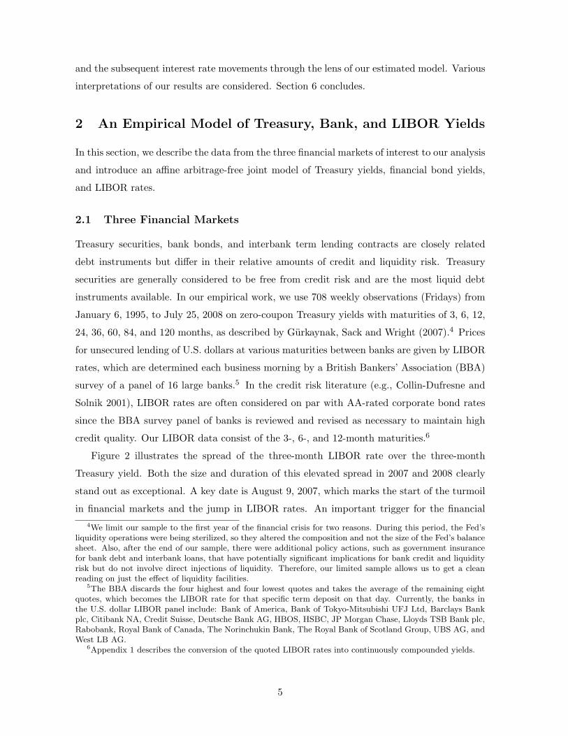
Figure 2 illustrates the spread of the three-month LIBOR rate over the three-month

Treasury yield. Both the size and duration of this elevated spread in 2007 and 2008 clearly

stand out as exceptional. A key date is August 9, 2007, which marks the start of the turmoil

in financial markets and the jump in LIBOR rates. An important trigger for the financial4We limit our sample to the first year of the financial crisis for two reasons. During this period, the Fed’s

liquidity operations were being sterilized, so they altered the composition and not the size of the Fed’s balancesheet. Also, after the end of our sample, there were additional policy actions, such as government insurancefor bank debt and interbank loans, that have potentially significant implications for bank credit and liquidityrisk but do not involve direct injections of liquidity. Therefore, our limited sample allows us to get a cleanreading on just the effect of liquidity facilities.

5The BBA discards the four highest and four lowest quotes and takes the average of the remaining eightquotes, which becomes the LIBOR rate for that specific term deposit on that day. Currently, the banks inthe U.S. dollar LIBOR panel include: Bank of America, Bank of Tokyo-Mitsubishi UFJ Ltd, Barclays Bankplc, Citibank NA, Credit Suisse, Deutsche Bank AG, HBOS, HSBC, JP Morgan Chase, Lloyds TSB Bank plc,Rabobank, Royal Bank of Canada, The Norinchukin Bank, The Royal Bank of Scotland Group, UBS AG, andWest LB AG.

6Appendix 1 describes the conversion of the quoted LIBOR rates into continuously compounded yields.

5

1996 1998 2000 2002 2004 2006 2008

−50

050

100

150

Spr

ead

in b

asis

poi

nts

Figure 2: Spread of Three-Month LIBOR rate over the Treasury Yield.This figure shows the weekly spread of the three-month LIBOR rate over the three-monthTreasury bond yield from January 6, 1995 to July 25, 2008.

crisis and the tightening of the money markets was the announcement by the French bank

BNP Paribas that it would suspend redemptions from three of its investment funds.7 The

mean spread in our sample prior to August 10, 2007, is about 25 basis points, while after

that date, the mean spread is 98 basis points.8 Fluctuations in the LIBOR-Treasury spread

are commonly attributed to movements in credit and liquidity risk premiums.9 The credit

risk premium compensates for the possibility that the borrowing bank will default. The7The BNP Paribas press release stated that “the complete evaporation of liquidity in certain market seg-

ments of the U.S. securitization market has made it impossible to value certain assets fairly regardless of theirquality or credit rating ... during these exceptional times, BNP Paribas has decided to temporarily suspendthe calculation of the net asset value as well as subscriptions/redemptions.”

8Data on the LIBOR-Treasury spread and on a very similar spread, the well-known eurodollar to Treasury(or TED) yield spread, can be obtained earlier than the 1995 start of our estimation sample (which is determinedby the availability of bank debt rates). Even in comparison to these earlier periods, the recent episode standsout as extraordinary.

9The LIBOR-Treasury spread is also affected by changes in the “convenience yield” for holding Treasurysecurities; therefore, Feldhutter and Lando (2008) and others use swap rates as an alternative riskless ratebenchmark that is free from idiosyncratic Treasury movements. However, because we focus on the dynamicinteractions between bank bond yields and LIBOR rates, the choice of the risk-free rate is not an issue for ouranalysis. Also note that seasonality issues, such as examined by Neely and Winters (2006), should not be anissue for our analysis since our LIBOR rates have maturities greater than one month.

6

liquidity risk premium is compensation for tying up funds in loans that—unlike liquid Treasury

securities—cannot easily be unwound before the loan matures. Importantly, liquidity risk

depends on the expected size of the idiosyncratic and aggregate liquidity shocks that effect

both the lender and borrower.10 Specifically, in the interbank market, borrowing and lending

banks worry about their ability to obtain ready funds during the term of the loan, and each

may desire a precautionary liquidity buffer.

To shed some light on the extent to which the jump in LIBOR rates represented an

increase in liquidity risk or in credit risk, our empirical analysis compares these rates to

yields on the unsecured bonds of U.S. financial institutions. We obtain zero-coupon yields on

the bond debt of U.S. banks and financial corporations from Bloomberg at the eight Treasury

maturities listed above. Our empirical model will estimate the amount of risk associated with

this financial debt by pooling across five different categories: A-rated and AA-rated financial

corporate debt, and BBB-, A-, and AA-rated bank debt.11 Yields for the first four types

of debt are available for our entire 1995-2008 sample, while yields on AA-rated bank debt

are only available after August 2001. At comparable maturities, LIBOR rates and yields on

AA-rated bank debt should be very close because both represent the cost of lending unsecured

funds to similar institutions. Indeed, for much of our sample, these rates are almost identical.

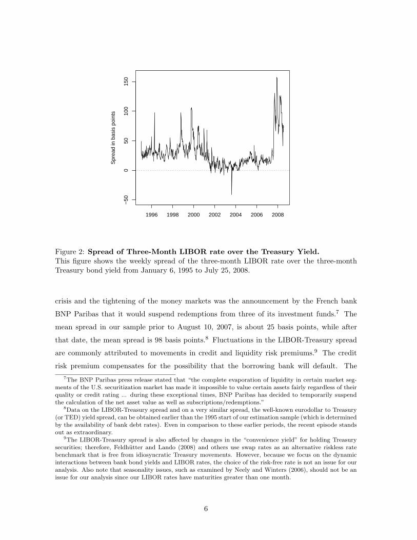
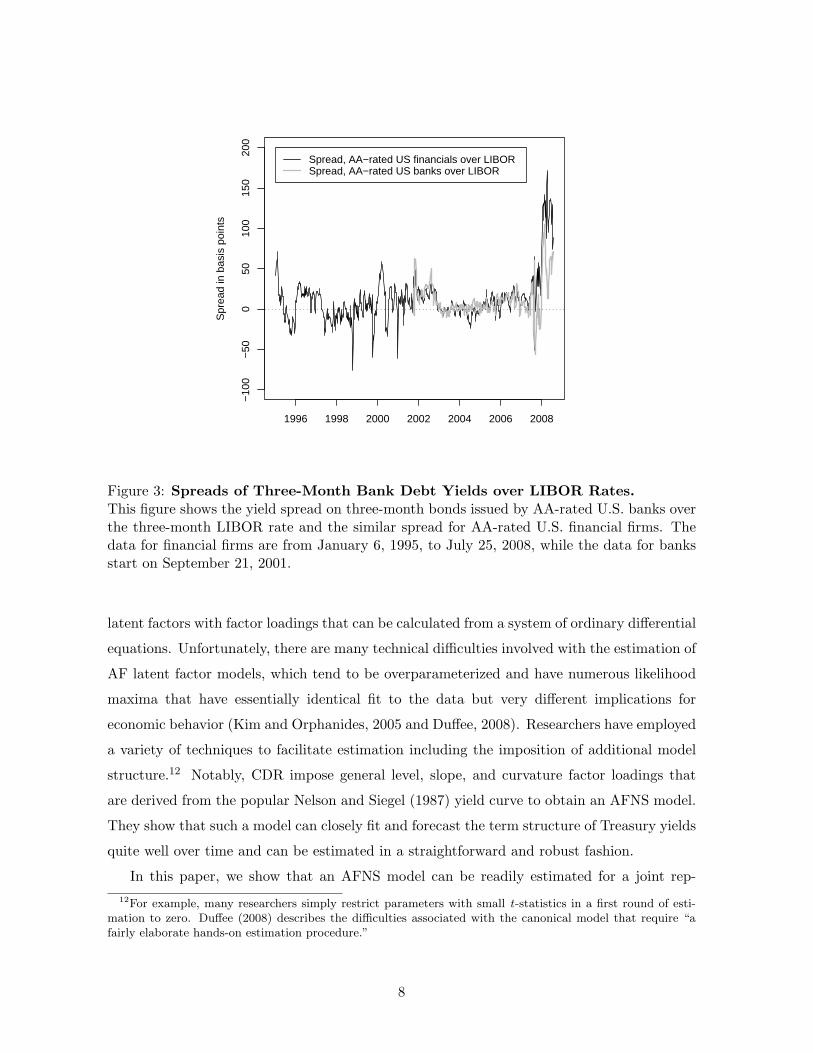
As shown in Figure 3, at a three-month maturity, the spread of the AA-rated bank debt yield

over the LIBOR rate and the spread of the AA-rated financial corporate debt yield over the

LIBOR rate are typically very close to zero. Furthermore, most deviations—say, in 2001 and

2002—were short-lived; therefore, financial bond debt and interbank loans appear to have

had very similar credit and liquidity risk characteristics. Of course, there was a persistent

and exceptional deviation that started at the end of 2007 during which the LIBOR fell below

the yield on comparable financial corporate debt. We provide empirical evidence in Section

5 that the relatively low rate on interbank borrowing after December 12, 2007, reflected the

extraordinary commitment by central banks to provide liquidity to the interbank market.

2.2 Six-factor AFNS Model

In this subsection, we introduce a joint affine AF model of Treasury yields, financial bond

yields, and LIBOR rates. Following Duffie and Kan (1996), affine AF term structure models

have been very popular, especially because yields are convenient linear functions of underlying10The underlying liquidity risk is systemic in nature, as in Li, et al. (2009); that is, the borrowing or lending

bank may be unable to sell sufficient quantities of assets in a timely manner and at a low cost, especiallywithout a significant adverse effect on market prices.

11Appendix 1 describes the conversion of the reported interest rates into continuously compounded yields.For more information on the Bloomberg data, see Feldhutter and Lando (2008).

7

1996 1998 2000 2002 2004 2006 2008

−10

0−

500

5010

015

020

0

Spr

ead

in b

asis

poi

nts

Spread, AA−rated US financials over LIBOR Spread, AA−rated US banks over LIBOR

Figure 3: Spreads of Three-Month Bank Debt Yields over LIBOR Rates.This figure shows the yield spread on three-month bonds issued by AA-rated U.S. banks overthe three-month LIBOR rate and the similar spread for AA-rated U.S. financial firms. Thedata for financial firms are from January 6, 1995, to July 25, 2008, while the data for banksstart on September 21, 2001.

latent factors with factor loadings that can be calculated from a system of ordinary differential

equations. Unfortunately, there are many technical difficulties involved with the estimation of

AF latent factor models, which tend to be overparameterized and have numerous likelihood

maxima that have essentially identical fit to the data but very different implications for

economic behavior (Kim and Orphanides, 2005 and Duffee, 2008). Researchers have employed

a variety of techniques to facilitate estimation including the imposition of additional model

structure.12 Notably, CDR impose general level, slope, and curvature factor loadings that

are derived from the popular Nelson and Siegel (1987) yield curve to obtain an AFNS model.

They show that such a model can closely fit and forecast the term structure of Treasury yields

quite well over time and can be estimated in a straightforward and robust fashion.

In this paper, we show that an AFNS model can be readily estimated for a joint rep-12For example, many researchers simply restrict parameters with small t-statistics in a first round of esti-

mation to zero. Duffee (2008) describes the difficulties associated with the canonical model that require “afairly elaborate hands-on estimation procedure.”

8

resentation of Treasury, bank bond, and LIBOR yields.13 Researchers have typically found

that three factors—typically referred to as level, slope, and curvature—are sufficient to model

the time-variation in the cross-section of nominal Treasury bond yields (e.g., Litterman and

Scheinkman, 1991). Similarly, we use a three-factor representation for Treasury yields. The

most general joint model of Treasury, bank bond, and LIBOR rates would add three more

factors for the bank bond yield curve and another three for the LIBOR rates of various ma-

turities. However, this nine-factor model is unlikely to be the most parsimonious empirical

representation, for as noted in the previous section, movements in Treasury, bank bond, and

LIBOR rates all share common elements.

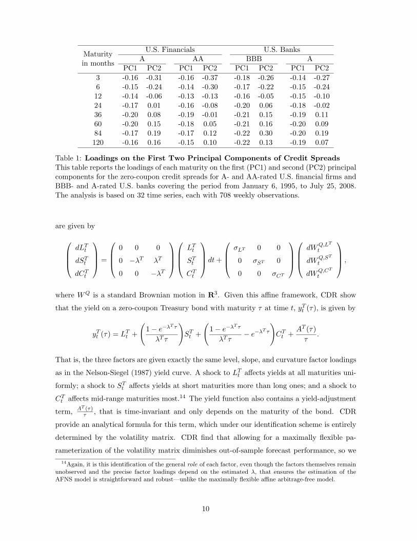
Some evidence on the number of additional factors required to capture variation in fi-

nancial bond yields can be obtained from their principal components. We subtract the bond

yields for the four categories of debt that are available for our complete sample (i.e., A-rated

and AA-rated financial corporate debt and BBB- and A-rated bank debt) from comparable-

maturity Treasury yields and calculate the first two principal components for these 32 yield

spreads (i.e., four rating-industry categories times eight maturities). The first two principal

components account for 85.5 and 8.8 percent, respectively, of the observed variation in the

bank debt yield spreads. The associated 32 factor loadings for these principal components are

reported in Table 1. The first principal component has very similar loadings across various

maturities so it can be viewed as a level factor. In contrast, the loadings of the second principal

component monotonically increase with maturity, which suggests a slope factor. Therefore,

we include two spread factors in our model to account for differences between bank debt yields

and Treasuries, which is also supported by evidence in Driessen (2005) and Christensen and

Lopez (2008). Finally, as in Feldhutter and Lando (2008), a single LIBOR factor appears

likely to be able to capture the small deviations between LIBOR rates and bank debt yields.

Therefore, our joint representation has six factors: three for nominal Treasury bond yields,

two additional ones for financial bond rate spreads, and finally, a sixth factor to capture

idiosyncratic variation in LIBOR rates.

Specifically, Treasury yields depend on a state vector of the three nominal factors (i.e.,

level, slope, and curvature) denoted as XTt = (LT

t , STt , CT

t ). The instantaneous risk-free rate

is given by

rTt = LT

t + STt ,

while the dynamics of the three state variables under the risk-neutral (or Q) pricing measure13In related work, Christensen, Lopez, and Rudebusch (2008) show that a four-factor AFNS model provides

a tractable and robust joint empirical model of nominal and real Treasury yield curves.

9

U.S. Financials U.S. BanksMaturityA AA BBB Ain months

PC1 PC2 PC1 PC2 PC1 PC2 PC1 PC23 -0.16 -0.31 -0.16 -0.37 -0.18 -0.26 -0.14 -0.276 -0.15 -0.24 -0.14 -0.30 -0.17 -0.22 -0.15 -0.2412 -0.14 -0.06 -0.13 -0.13 -0.16 -0.05 -0.15 -0.1024 -0.17 0.01 -0.16 -0.08 -0.20 0.06 -0.18 -0.0236 -0.20 0.08 -0.19 -0.01 -0.21 0.15 -0.19 0.1160 -0.20 0.15 -0.18 0.05 -0.21 0.16 -0.20 0.0984 -0.17 0.19 -0.17 0.12 -0.22 0.30 -0.20 0.19120 -0.16 0.16 -0.15 0.10 -0.22 0.13 -0.19 0.07

Table 1: Loadings on the First Two Principal Components of Credit SpreadsThis table reports the loadings of each maturity on the first (PC1) and second (PC2) principalcomponents for the zero-coupon credit spreads for A- and AA-rated U.S. financial firms andBBB- and A-rated U.S. banks covering the period from January 6, 1995, to July 25, 2008.The analysis is based on 32 time series, each with 708 weekly observations.

are given by

dLTt

dSTt

dCTt

=

0 0 0

0 −λT λT

0 0 −λT

LTt

STt

CTt

dt +

σLT 0 0

0 σST 0

0 0 σCT

dWQ,LT

t

dWQ,ST

t

dWQ,CT

t

,

where WQ is a standard Brownian motion in R3. Given this affine framework, CDR show

that the yield on a zero-coupon Treasury bond with maturity τ at time t, yTt (τ), is given by

yTt (τ) = LT

t +

(1− e−λT τ

λT τ

)ST

t +

(1− e−λT τ

λT τ− e−λT τ

)CT

t +AT (τ)

τ.

That is, the three factors are given exactly the same level, slope, and curvature factor loadings

as in the Nelson-Siegel (1987) yield curve. A shock to LTt affects yields at all maturities uni-

formly; a shock to STt affects yields at short maturities more than long ones; and a shock to

CTt affects mid-range maturities most.14 The yield function also contains a yield-adjustment

term, AT (τ)τ , that is time-invariant and only depends on the maturity of the bond. CDR

provide an analytical formula for this term, which under our identification scheme is entirely

determined by the volatility matrix. CDR find that allowing for a maximally flexible pa-

rameterization of the volatility matrix diminishes out-of-sample forecast performance, so we14Again, it is this identification of the general role of each factor, even though the factors themselves remain

unobserved and the precise factor loadings depend on the estimated λ, that ensures the estimation of theAFNS model is straightforward and robust—unlike the maximally flexible affine arbitrage-free model.

10

restrict it to be diagonal.15

To incorporate bond yields for U.S. banks and financial firms into this structure, we follow

Christensen and Lopez (2008). Namely, the instantaneous discount rate for corporate bonds

from industry i (bank or financial corporation) with rating c (BBB, A, or AA) is assumed to

be

ri,ct = αi,c

0 +(1 + αi,c

LT

)LT

t +(1 + αi,c

ST

)ST

t +(αi,c

LS

)LS

t +(αi,c

SS

)SS

t ,

where(LT

t , STt

)are the Treasury factors described above and

(LS

t , SSt

)are two bank debt

yield spread factors. The instantaneous credit spread over the instantaneous risk-free Treasury

rate becomes

si,ct ≡ ri,c

t − rTt

= αi,c0 +

(αi,c

LT

)LT

t +(αi,c

ST

)ST

t +(αi,c

LS

)LS

t +(αi,c

SS

)SS

t .

Note that the sensitivity of these risk factors can be adjusted by varying the αi,c parameters,

which is consistent with the pattern observed in the principal component analysis of the yield

spreads in Table 1.16

To obtain the desired Nelson-Siegel level and slope factor-loading structure for the two

bank yield spread factors, their dynamics under the pricing measure are given by

dLSt

dSSt

dLTt

dSTt

dCTt

=

0 0 0 0 0

0 −λS 0 0 0

0 0 0 0 0

0 0 0 −λT λT

0 0 0 0 −λT

LSt

SSt

LTt

STt

CTt

dt + ΣS

dWQ,LS

t

dWQ,SS

t

dWQ,LT

t

dWQ,ST

t

dWQ,CT

t

,

where ΣS is a diagonal matrix, since the two common credit risk factors are assumed to be

independent of the three factors determining the risk-free rate. This structure delivers the

desired Nelson-Siegel factor loadings for all five factors in the corporate bond yield function.

As a result, the yield on a corporate zero-coupon bond from industry i with rating c and15We have fixed the mean under the Q-measure at zero, without loss of generality. The AFNS model

dynamics under the Q-measure may appear restrictive, but CDR show this structure coupled with general riskpricing provides a very flexible modeling structure.

16Note that for each rating category, we do not take rating transitions into consideration. This is a theoreticalinconsistency of our approach, but the model will extract common risk factors across rating categories andbusiness sectors if they are present in the data. Taking the rating transitions into consideration will not changeour results in a significant way. The model framework does allow for such extensions; for example, the methodused by Feldhutter and Lando (2008) can be applied in this setting under the restriction that each ratingcategory has the same factor loading on the two common credit risk factors. We leave this for future research.

11

maturity τ is given by

yi,ct (τ) =

(1 + αi,c

LT

)LT

t +(1 + αi,c

ST

)(1− e−λT τ

λT τ

)ST

t +(1 + αi,c

ST

)(1− e−λT τ

λT τ− e−λT τ

)CT

t

+αi,c0 +

(αi,c

LS

)LS

t +(αi,c

SS

)(1− e−λSτ

λSτ

)SS

t +Ai,c(τ)

τ,

where the yield-adjustment term Ai,c(τ)τ is time-invariant and depends only on the maturity

of the bond.

Finally, to account for idiosyncratic differences between U.S. dollar LIBOR rates and

corporate bond yields paid by AA-rated U.S. financial institutions, we include a sixth factor

in the model for the discount rate applied to term loans in the interbank market. This

instantaneous discount rate is given by

rLibt = rFin,AA

t + αLib + XLibt ,

where the Q dynamics of the LIBOR-specific factor are assumed to be given by

dXLibt = −κQ

LibXLibt dt + σLibdWQ,Lib

t .

This factor is assumed to be independent of the other five factors under the pricing measure.

Thus, the full state vector, Xt = (LSt , SS

t , LTt , ST

t , CTt , XLib

t ), of the six-factor model has

assumed Q-dynamics:

dXt =

0 0 0 0 0 0

0 −λS 0 0 0 0

0 0 0 0 0 0

0 0 0 −λT λT 0

0 0 0 0 −λT 0

0 0 0 0 0 −κQLib

Xtdt + ΣLib

dWQ,LS

t

dWQ,SS

t

dWQ,LT

t

dWQ,ST

t

dWQ,CT

t

dWQ,Libt

,

where ΣLib is a diagonal matrix. The discount rate to be applied to LIBOR contracts is then

rLibt = rFin,AA

t + αLib + XLibt

= αFin,AA0 +

(1 + αFin,AA

LT

)LT

t +(1 + αFin,AA

ST

)ST

t +(αFin,AA

LS

)LS

t +(αFin,AA

SS

)SS

t + αLib + XLibt .

12

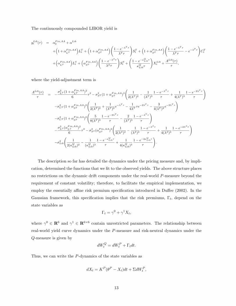
The continuously compounded LIBOR yield is

yLibt (τ) = αFin,AA

0 + αLib

+(1 + αFin,AA

LT

)LT

t +(1 + αFin,AA

ST

)(1− e−λT τ

λT τ

)ST

t +(1 + αFin,AA

ST

)(1− e−λT τ

λT τ− e−λT τ

)CT

t

+(αFin,AA

LS

)LS

t +(αFin,AA

SS

)(1− e−λSτ

λSτ

)SS

t +

(1− e−κ

QLib

τ

κQLibτ

)XLib

t +ALib(τ)

τ,

where the yield-adjustment term is

ALib(τ)

τ= −σ2

LT (1 + αFin,AA

LT )2

6τ2 − σ2

ST (1 + αFin,AA

ST )2(

1

2(λT )2− 1

(λT )31− e−λT τ

τ+

1

4(λT )31− e−2λT τ

τ

)

−σ2CT (1 + αFin,AA

ST )2(

1

2(λT )2+

1

(λT )2e−λT τ − 1

4λTτe−2λT τ − 3

4(λT )2e−2λT τ

)

−σ2CT (1 + αFin,AA

ST )2(

5

8(λT )31− e−2λT τ

τ− 2

(λT )31− e−λT τ

τ

)

−σ2LS (αFin,AA

LS )2

6τ2 − σ2

SS (αFin,AA

SS )2(

1

2(λS)2− 1

(λS)31− e−λSτ

τ+

1

4(λS)31− e−2λSτ

τ

)

−σ2Lib

(1

2(κQLib)

2− 1

(κQLib)

3

1− e−κQLib

τ

τ+

1

4(κQLib)

3

1− e−2κQLib

τ

τ

).

The description so far has detailed the dynamics under the pricing measure and, by impli-

cation, determined the functions that we fit to the observed yields. The above structure places

no restrictions on the dynamic drift components under the real-world P -measure beyond the

requirement of constant volatility; therefore, to facilitate the empirical implementation, we

employ the essentially affine risk premium specification introduced in Duffee (2002). In the

Gaussian framework, this specification implies that the risk premiums, Γt, depend on the

state variables as

Γt = γ0 + γ1Xt,

where γ0 ∈ R6 and γ1 ∈ R6×6 contain unrestricted parameters. The relationship between

real-world yield curve dynamics under the P -measure and risk-neutral dynamics under the

Q-measure is given by

dWQt = dWP

t + Γtdt.

Thus, we can write the P -dynamics of the state variables as

dXt = KP (θP −Xt)dt + ΣdWPt ,

13

where both KP and θP are allowed to vary freely relative to their counterparts under the

Q-measure.

3 Model estimation

This section first describes our Kalman filter estimation procedure for the AFNS joint model

of Treasury, bank debt, and LIBOR rates and then provides estimation results.

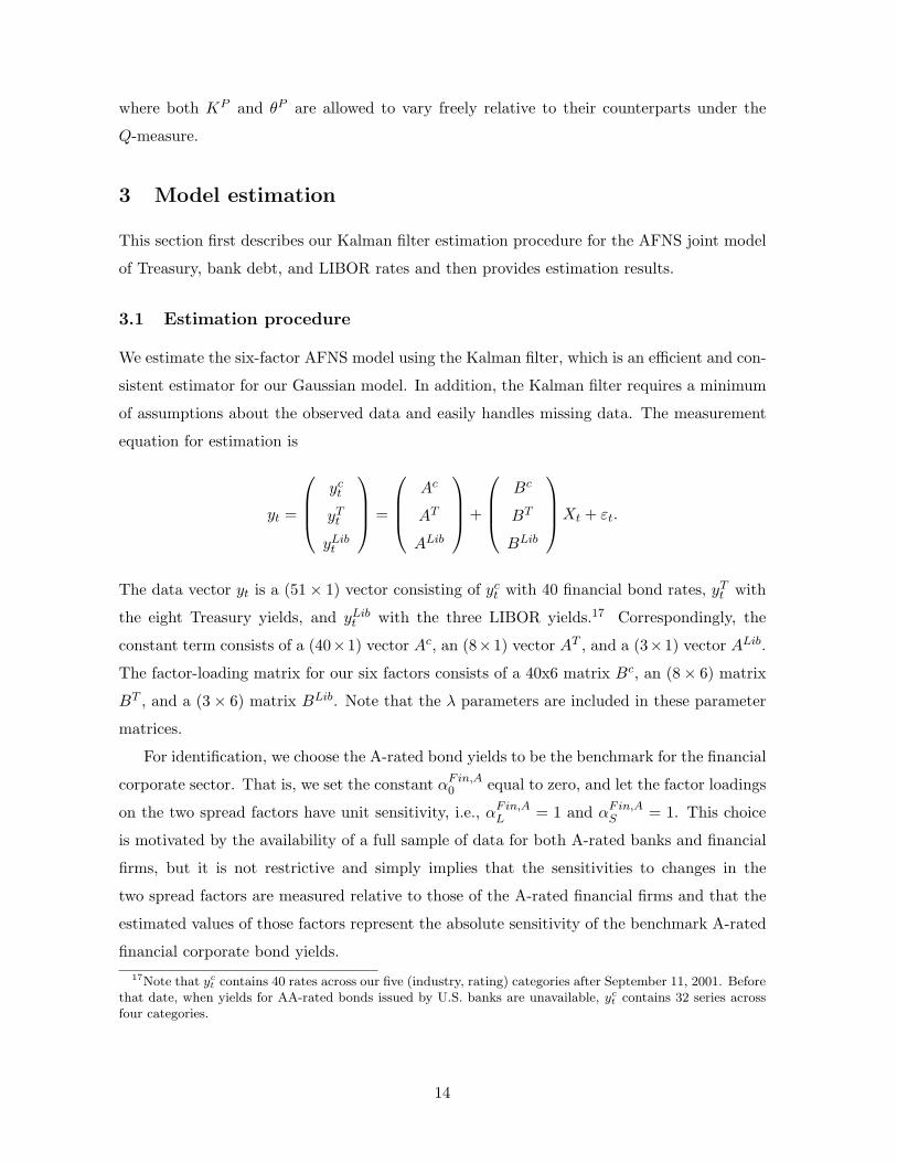
3.1 Estimation procedure

We estimate the six-factor AFNS model using the Kalman filter, which is an efficient and con-

sistent estimator for our Gaussian model. In addition, the Kalman filter requires a minimum

of assumptions about the observed data and easily handles missing data. The measurement

equation for estimation is

yt =

yct

yTt

yLibt

=

Ac

AT

ALib

+

Bc

BT

BLib

Xt + εt.

The data vector yt is a (51× 1) vector consisting of yct with 40 financial bond rates, yT

t with

the eight Treasury yields, and yLibt with the three LIBOR yields.17 Correspondingly, the

constant term consists of a (40×1) vector Ac, an (8×1) vector AT , and a (3×1) vector ALib.

The factor-loading matrix for our six factors consists of a 40x6 matrix Bc, an (8× 6) matrix

BT , and a (3× 6) matrix BLib. Note that the λ parameters are included in these parameter

matrices.

For identification, we choose the A-rated bond yields to be the benchmark for the financial

corporate sector. That is, we set the constant αFin,A0 equal to zero, and let the factor loadings

on the two spread factors have unit sensitivity, i.e., αFin,AL = 1 and αFin,A

S = 1. This choice

is motivated by the availability of a full sample of data for both A-rated banks and financial

firms, but it is not restrictive and simply implies that the sensitivities to changes in the

two spread factors are measured relative to those of the A-rated financial firms and that the

estimated values of those factors represent the absolute sensitivity of the benchmark A-rated

financial corporate bond yields.17Note that yc

t contains 40 rates across our five (industry, rating) categories after September 11, 2001. Beforethat date, when yields for AA-rated bonds issued by U.S. banks are unavailable, yc

t contains 32 series acrossfour categories.

14

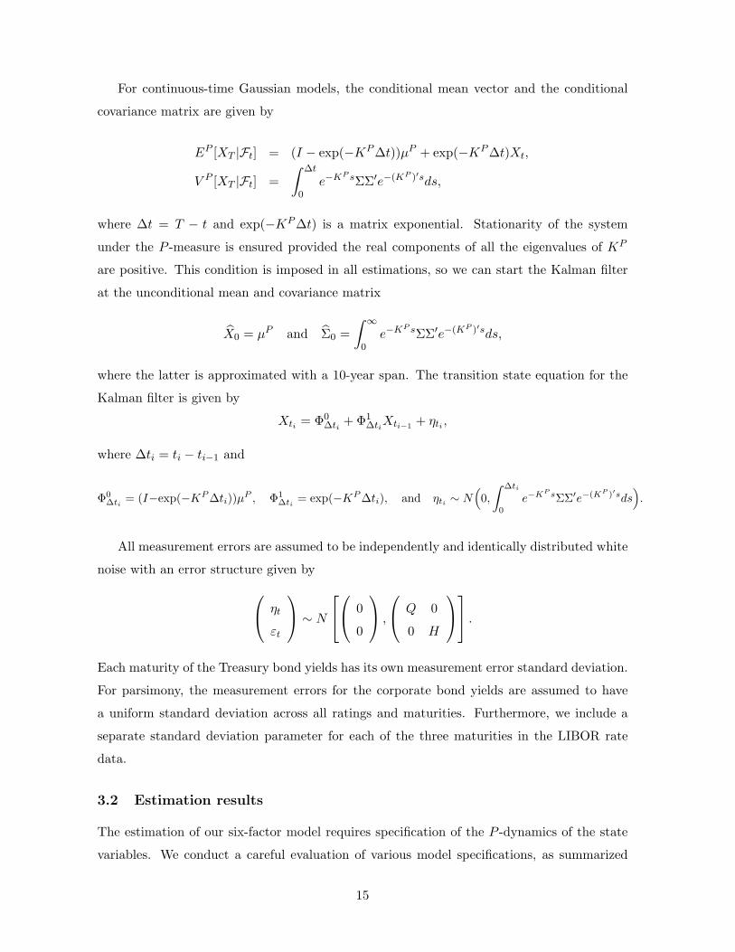
For continuous-time Gaussian models, the conditional mean vector and the conditional

covariance matrix are given by

EP [XT |Ft] = (I − exp(−KP ∆t))µP + exp(−KP ∆t)Xt,

V P [XT |Ft] =∫ ∆t

0e−KP sΣΣ′e−(KP )′sds,

where ∆t = T − t and exp(−KP ∆t) is a matrix exponential. Stationarity of the system

under the P -measure is ensured provided the real components of all the eigenvalues of KP

are positive. This condition is imposed in all estimations, so we can start the Kalman filter

at the unconditional mean and covariance matrix

X0 = µP and Σ0 =∫ ∞

0e−KP sΣΣ′e−(KP )′sds,

where the latter is approximated with a 10-year span. The transition state equation for the

Kalman filter is given by

Xti = Φ0∆ti + Φ1

∆tiXti−1 + ηti ,

where ∆ti = ti − ti−1 and

Φ0∆ti

= (I−exp(−KP ∆ti))µP , Φ1∆ti

= exp(−KP ∆ti), and ηti ∼ N(0,

∫ ∆ti

0

e−KP sΣΣ′e−(KP )′sds).

All measurement errors are assumed to be independently and identically distributed white

noise with an error structure given by

ηt

εt

∼ N

0

0

,

Q 0

0 H

.

Each maturity of the Treasury bond yields has its own measurement error standard deviation.

For parsimony, the measurement errors for the corporate bond yields are assumed to have

a uniform standard deviation across all ratings and maturities. Furthermore, we include a

separate standard deviation parameter for each of the three maturities in the LIBOR rate

data.

3.2 Estimation results

The estimation of our six-factor model requires specification of the P -dynamics of the state

variables. We conduct a careful evaluation of various model specifications, as summarized

15

Alternative Goodness of fit statisticsSpecifications log L k p-value BIC(1) Unrestricted KP 180,171.90 86 n.a. -359,779.4(2) κP

35 = 0 180,171.86 85 0.7773 -359,785.9(3) κP

35 = κP16 = 0 180,171.82 84 0.7773 -359,792.4

(4) κP35 = κP

16 = κP23 = 0 180,171.80 83 0.8415 -359,798.9

(5) κP35 = · · · = κP

41 = 0 180,171.68 82 0.6242 -359,805.2(6) κP

35 = · · · = κP63 = 0 180,171.58 81 0.6547 -359,811.6

(7) κP35 = · · · = κP

13 = 0 180,171.47 80 0.6390 -359,817.9(8) κP

35 = · · · = κP24 = 0 180,171.31 79 0.5716 -359,824.2

(9) κP35 = · · · = κP

54 = 0 180,171.01 78 0.4386 -359,830.1(10) κP

35 = · · · = κP34 = 0 180,170.51 77 0.3173 -359,835.7

(11) κP35 = · · · = κP

32 = 0 180,170.47 76 0.7773 -359,842.2(12) κP

35 = · · · = κP36 = 0 180,170.25 75 0.5071 -359,848.3

(13) κP35 = · · · = κP

53 = 0 180,169.37 74 0.1846 -359,853.1(14) κP

35 = · · · = κP14 = 0 180,167.84 73 0.0802 -359,856.6

(15) κP35 = · · · = κP

15 = 0 180,167.15 72 0.2401 -359,861.8(16) κP

35 = · · · = κP42 = 0 180,166.20 71 0.1681 -359,866.5

(17) κP35 = · · · = κP

52 = 0 180,165.23 70 0.1637 -359,871.1(18) κP

35 = · · · = κP51 = 0 180,162.42 69 0.0178 -359,872.0

(19) κP35 = · · · = κP

31 = 0 180,160.46 68 0.0477 -359,874.7(20) κP

35 = · · · = κP43 = 0 180,153.73 67 0.0003 -359,867.8

(21) κP35 = · · · = κP

21 = 0 180,149.97 66 0.0061 -359,866.8(22) κP

35 = · · · = κP65 = 0 180,146.25 65 0.0064 -359,865.9

(23) κP35 = · · · = κP

46 = 0 180,142.61 64 0.0070 -359,865.2(24) κP

35 = · · · = κP56 = 0 180,135.02 63 0.0001 -359,856.6

(25) κP35 = · · · = κP

25 = 0 180,125.40 62 < 0.0001 -359,843.9(26) κP

35 = · · · = κP64 = 0 180,111.52 61 < 0.0001 -359,822.7

(27) κP35 = · · · = κP

26 = 0 180,083.20 60 < 0.0001 -359,772.7(28) κP

35 = · · · = κP12 = 0 180,079.76 59 0.0087 -359,772.3

(29) κP35 = · · · = κP

45 = 0 180,059.29 58 < 0.0001 -359,738.0(30) κP

35 = · · · = κP62 = 0 180,043.08 57 < 0.0001 -359,712.1

(31) κP35 = · · · = κP

61 = 0 180,038.57 56 0.0027 -359,709.6

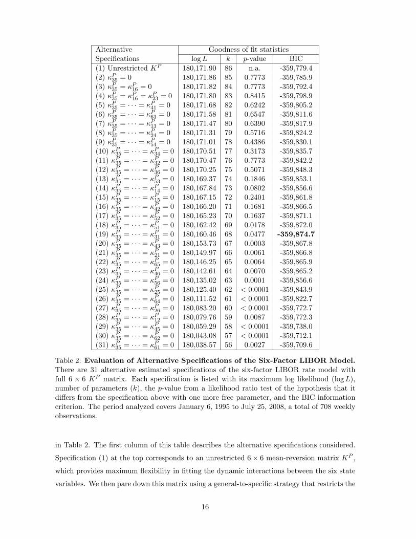
Table 2: Evaluation of Alternative Specifications of the Six-Factor LIBOR Model.There are 31 alternative estimated specifications of the six-factor LIBOR rate model withfull 6 × 6 KP matrix. Each specification is listed with its maximum log likelihood (log L),number of parameters (k), the p-value from a likelihood ratio test of the hypothesis that itdiffers from the specification above with one more free parameter, and the BIC informationcriterion. The period analyzed covers January 6, 1995 to July 25, 2008, a total of 708 weeklyobservations.

in Table 2. The first column of this table describes the alternative specifications considered.

Specification (1) at the top corresponds to an unrestricted 6× 6 mean-reversion matrix KP ,

which provides maximum flexibility in fitting the dynamic interactions between the six state

variables. We then pare down this matrix using a general-to-specific strategy that restricts the

16

KP KP·,1 KP

·,2 KP·,3 KP

·,4 KP·,5 KP

·,6 θP ΣKP

1,· -1.084 -1.232 0 0 0 0 0.01332 0.001876(0.152) (0.200) (0.00766) (0.000111)

KP2,· 0.6535 0.3596 0 0 0.1560 -1.170 -0.009623 0.002006

(0.303) (0.295) (0.0498) (0.541) (0.00672) (0.000180)KP

3,· 0 0 0.05506 0 0 0 0.06669 0.004781(0.188) (0.0194) (0.000121)

KP4,· 0 0 1.155 0.9203 -1.127 -2.807 -0.03003 0.008242

(0.583) (0.185) (0.173) (1.38) (0.0194) (0.000235)KP

5,· 0 0 0 0 0.7677 13.31 -0.01803 0.02647(0.503) (4.14) (0.00842) (0.000631)

KP6,· 3.763 4.574 0 -0.3537 -0.2235 8.939 0.05616 0.004704

(0.688) (0.728) (0.141) (0.0991) (1.35) (0.118) (0.000239)

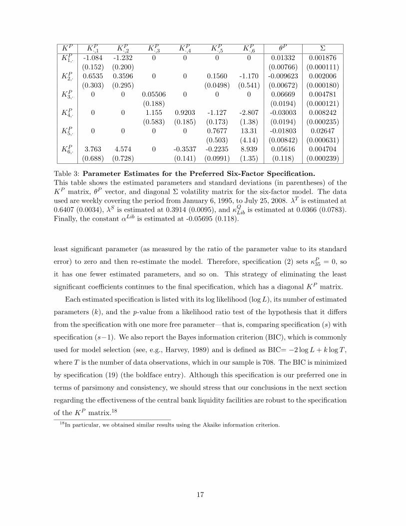
Table 3: Parameter Estimates for the Preferred Six-Factor Specification.This table shows the estimated parameters and standard deviations (in parentheses) of theKP matrix, θP vector, and diagonal Σ volatility matrix for the six-factor model. The dataused are weekly covering the period from January 6, 1995, to July 25, 2008. λT is estimated at0.6407 (0.0034), λS is estimated at 0.3914 (0.0095), and κQ

Lib is estimated at 0.0366 (0.0783).Finally, the constant αLib is estimated at -0.05695 (0.118).

least significant parameter (as measured by the ratio of the parameter value to its standard

error) to zero and then re-estimate the model. Therefore, specification (2) sets κP35 = 0, so

it has one fewer estimated parameters, and so on. This strategy of eliminating the least

significant coefficients continues to the final specification, which has a diagonal KP matrix.

Each estimated specification is listed with its log likelihood (log L), its number of estimated

parameters (k), and the p-value from a likelihood ratio test of the hypothesis that it differs

from the specification with one more free parameter—that is, comparing specification (s) with

specification (s−1). We also report the Bayes information criterion (BIC), which is commonly

used for model selection (see, e.g., Harvey, 1989) and is defined as BIC= −2 log L + k log T ,

where T is the number of data observations, which in our sample is 708. The BIC is minimized

by specification (19) (the boldface entry). Although this specification is our preferred one in

terms of parsimony and consistency, we should stress that our conclusions in the next section

regarding the effectiveness of the central bank liquidity facilities are robust to the specification

of the KP matrix.18

18In particular, we obtained similar results using the Akaike information criterion.

17

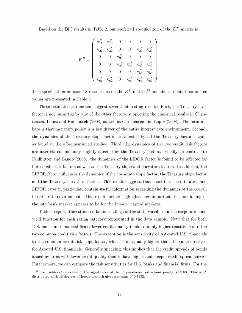
Based on the BIC results in Table 2, our preferred specification of the KP matrix is

KP =

κP11 κP

12 0 0 0 0

κP21 κP

22 0 0 κP25 κP

26

0 0 κP33 0 0 0

0 0 κP43 κP

44 κP45 κP

46

0 0 0 0 κP55 κP

56

κP61 κP

62 0 κP64 κP

65 κP66

.

This specification imposes 18 restrictions on the KP matrix,19 and the estimated parameter

values are presented in Table 3.

These estimated parameters suggest several interesting results. First, the Treasury level

factor is not impacted by any of the other factors, supporting the empirical results in Chris-

tensen, Lopez and Rudebusch (2008) as well as Christensen and Lopez (2008). The intuition

here is that monetary policy is a key driver of the entire interest rate environment. Second,

the dynamics of the Treasury slope factor are affected by all the Treasury factors, again

as found in the aforementioned studies. Third, the dynamics of the two credit risk factors

are interrelated, but only slightly affected by the Treasury factors. Finally, in contrast to

Feldhutter and Lando (2008), the dynamics of the LIBOR factor is found to be affected by

both credit risk factors as well as the Treasury slope and curvature factors. In addition, the

LIBOR factor influences the dynamics of the corporate slope factor, the Treasury slope factor

and the Treasury curvature factor. This result suggests that short-term credit rates, and

LIBOR rates in particular, contain useful information regarding the dynamics of the overall

interest rate environment. This result further highlights how important the functioning of

the interbank market appears to be for the broader capital markets.

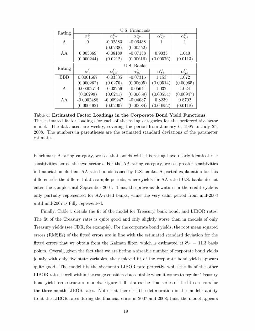
Table 4 reports the estimated factor loadings of the state variables in the corporate bond

yield function for each rating category represented in the data sample. Note that for both

U.S. banks and financial firms, lower credit quality tends to imply higher sensitivities to the

two common credit risk factors. The exception is the sensitivity of AA-rated U.S. financials

to the common credit risk slope factor, which is marginally higher than the value observed

for A-rated U.S. financials. Generally speaking, this implies that the credit spreads of bonds

issued by firms with lower credit quality tend to have higher and steeper credit spread curves.

Furthermore, we can compare the risk sensitivities for U.S. banks and financial firms. For the19The likelihood ratio test of the significance of the 18 parameter restrictions jointly is 22.88. This is χ2

distributed with 18 degrees of freedom which gives a p-value of 0.1952.

18

U.S. FinancialsRatingαC

0 αCLT αC

ST αCLS αC

SS

A 0 -0.02583 -0.06438 1 1(0.0238) (0.00552)

AA 0.003369 -0.08189 -0.07158 0.9033 1.040(0.000244) (0.0212) (0.00616) (0.00576) (0.0113)

U.S. BanksRatingαC

0 αCLT αC

ST αCLS αC

SS

BBB 0.0001667 -0.03335 -0.07316 1.153 1.072(0.000262) (0.0270) (0.00605) (0.00514) (0.00965)

A -0.00002714 -0.03256 -0.05644 1.032 1.024(0.00299) (0.0241) (0.00659) (0.00554) (0.00947)

AA -0.0002488 -0.009247 -0.04037 0.8239 0.8702(0.000492) (0.0200) (0.00684) (0.00852) (0.0118)

Table 4: Estimated Factor Loadings in the Corporate Bond Yield Functions.The estimated factor loadings for each of the rating categories for the preferred six-factormodel. The data used are weekly, covering the period from January 6, 1995 to July 25,2008. The numbers in parentheses are the estimated standard deviations of the parameterestimates.

benchmark A-rating category, we see that bonds with this rating have nearly identical risk

sensitivities across the two sectors. For the AA-rating category, we see greater sensitivities

in financial bonds than AA-rated bonds issued by U.S. banks. A partial explanation for this

difference is the different data sample periods, where yields for AA-rated U.S. banks do not

enter the sample until September 2001. Thus, the previous downturn in the credit cycle is

only partially represented for AA-rated banks, while the very calm period from mid-2003

until mid-2007 is fully represented.

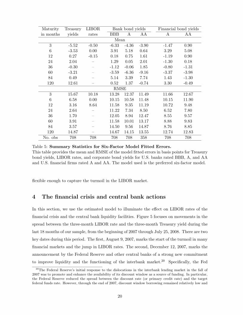
Finally, Table 5 details the fit of the model for Treasury, bank bond, and LIBOR rates.

The fit of the Treasury rates is quite good and only slightly worse than in models of only

Treasury yields (see CDR, for example). For the corporate bond yields, the root mean squared

errors (RMSEs) of the fitted errors are in line with the estimated standard deviation for the

fitted errors that we obtain from the Kalman filter, which is estimated at σεc = 11.3 basis

points. Overall, given the fact that we are fitting a sizeable number of corporate bond yields

jointly with only five state variables, the achieved fit of the corporate bond yields appears

quite good. The model fits the six-month LIBOR rate perfectly, while the fit of the other

LIBOR rates is well within the range considered acceptable when it comes to regular Treasury

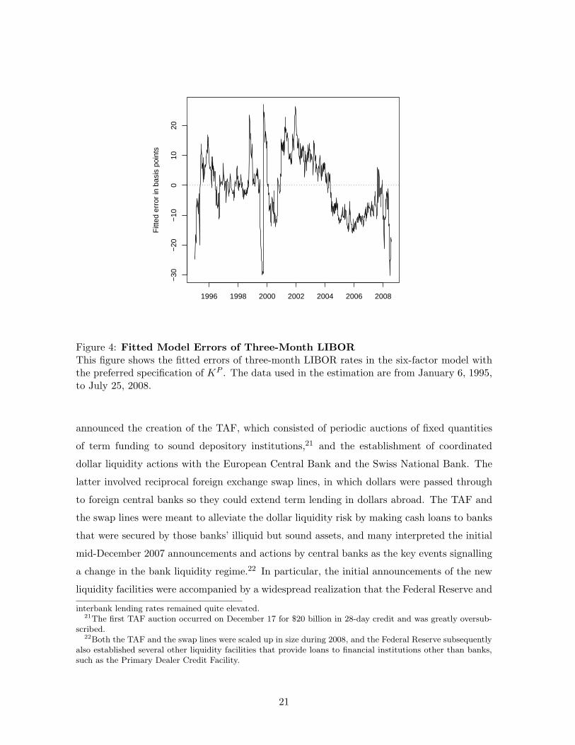
bond yield term structure models. Figure 4 illustrates the time series of the fitted errors for

the three-month LIBOR rates. Note that there is little deterioration in the model’s ability

to fit the LIBOR rates during the financial crisis in 2007 and 2008; thus, the model appears

19

Maturity Treasury LIBOR Bank bond yields Financial bond yieldsin months yields rates BBB A AA A AA

Mean3 -5.52 -0.50 -6.33 -4.36 -3.90 -1.47 0.906 -3.53 0.00 3.91 5.18 0.64 3.29 5.0812 0.27 -0.15 0.18 0.75 1.61 -1.19 0.9024 2.04 – 1.29 0.05 2.01 -1.30 0.1836 -0.30 – -1.12 -0.06 1.85 -0.80 -1.3160 -3.21 – -3.59 -6.36 -9.16 -3.37 -3.9884 0.49 – 5.14 3.39 7.74 1.43 -1.30120 12.61 – 0.52 1.37 -0.74 3.30 -0.49

RMSE3 15.67 10.18 13.28 12.37 11.49 11.66 12.676 6.58 0.00 10.15 10.58 11.48 10.15 11.9012 3.16 8.64 11.58 9.35 11.19 10.72 9.4824 2.64 – 11.22 7.34 8.50 6.52 7.8036 1.70 – 12.05 8.94 12.47 8.55 9.5760 3.91 – 11.58 10.01 13.17 8.88 9.8384 3.57 – 14.50 9.56 14.87 8.76 8.85120 14.87 – 14.67 14.15 13.55 12.74 12.83

No. obs 708 708 708 708 358 708 708

Table 5: Summary Statistics for Six-Factor Model Fitted Errors.This table provides the mean and RMSE of the model fitted errors in basis points for Treasurybond yields, LIBOR rates, and corporate bond yields for U.S. banks rated BBB, A, and AAand U.S. financial firms rated A and AA. The model used is the preferred six-factor model.

flexible enough to capture the turmoil in the LIBOR market.

4 The financial crisis and central bank actions

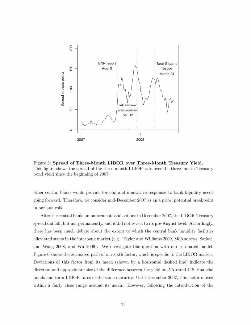
In this section, we use the estimated model to illuminate the effect on LIBOR rates of the

financial crisis and the central bank liquidity facilities. Figure 5 focuses on movements in the

spread between the three-month LIBOR rate and the three-month Treasury yield during the

last 18 months of our sample, from the beginning of 2007 through July 25, 2008. There are two

key dates during this period. The first, August 9, 2007, marks the start of the turmoil in many

financial markets and the jump in LIBOR rates. The second, December 12, 2007, marks the

announcement by the Federal Reserve and other central banks of a strong new commitment

to improve liquidity and the functioning of the interbank market.20 Specifically, the Fed20The Federal Reserve’s initial response to the dislocations in the interbank lending market in the fall of

2007 was to promote and enhance the availability of its discount window as a source of funding. In particular,the Federal Reserve reduced the spread between the discount rate (or primary credit rate) and the targetfederal funds rate. However, through the end of 2007, discount window borrowing remained relatively low and

20

1996 1998 2000 2002 2004 2006 2008

−30

−20

−10

010

20

Fitt

ed e

rror

in b

asis

poi

nts

Figure 4: Fitted Model Errors of Three-Month LIBORThis figure shows the fitted errors of three-month LIBOR rates in the six-factor model withthe preferred specification of KP . The data used in the estimation are from January 6, 1995,to July 25, 2008.

announced the creation of the TAF, which consisted of periodic auctions of fixed quantities

of term funding to sound depository institutions,21 and the establishment of coordinated

dollar liquidity actions with the European Central Bank and the Swiss National Bank. The

latter involved reciprocal foreign exchange swap lines, in which dollars were passed through

to foreign central banks so they could extend term lending in dollars abroad. The TAF and

the swap lines were meant to alleviate the dollar liquidity risk by making cash loans to banks

that were secured by those banks’ illiquid but sound assets, and many interpreted the initial

mid-December 2007 announcements and actions by central banks as the key events signalling

a change in the bank liquidity regime.22 In particular, the initial announcements of the new

liquidity facilities were accompanied by a widespread realization that the Federal Reserve and

interbank lending rates remained quite elevated.21The first TAF auction occurred on December 17 for $20 billion in 28-day credit and was greatly oversub-

scribed.22Both the TAF and the swap lines were scaled up in size during 2008, and the Federal Reserve subsequently

also established several other liquidity facilities that provide loans to financial institutions other than banks,such as the Primary Dealer Credit Facility.

21

2007 2008

050

100

150

200

Spr

ead

in b

asis

poi

nts

BNP reportAug. 9

TAF and swap

announcement

Dec. 12

Bear Stearnsrescue

March 24

Figure 5: Spread of Three-Month LIBOR over Three-Month Treasury Yield.This figure shows the spread of the three-month LIBOR rate over the three-month Treasurybond yield since the beginning of 2007.

other central banks would provide forceful and innovative responses to bank liquidity needs

going forward. Therefore, we consider mid-December 2007 as an a priori potential breakpoint

in our analysis.

After the central bank announcements and actions in December 2007, the LIBOR-Treasury

spread did fall, but not permanently, and it did not revert to its pre-August level. Accordingly,

there has been much debate about the extent to which the central bank liquidity facilities

alleviated stress in the interbank market (e.g., Taylor and Williams 2009, McAndrews, Sarkar,

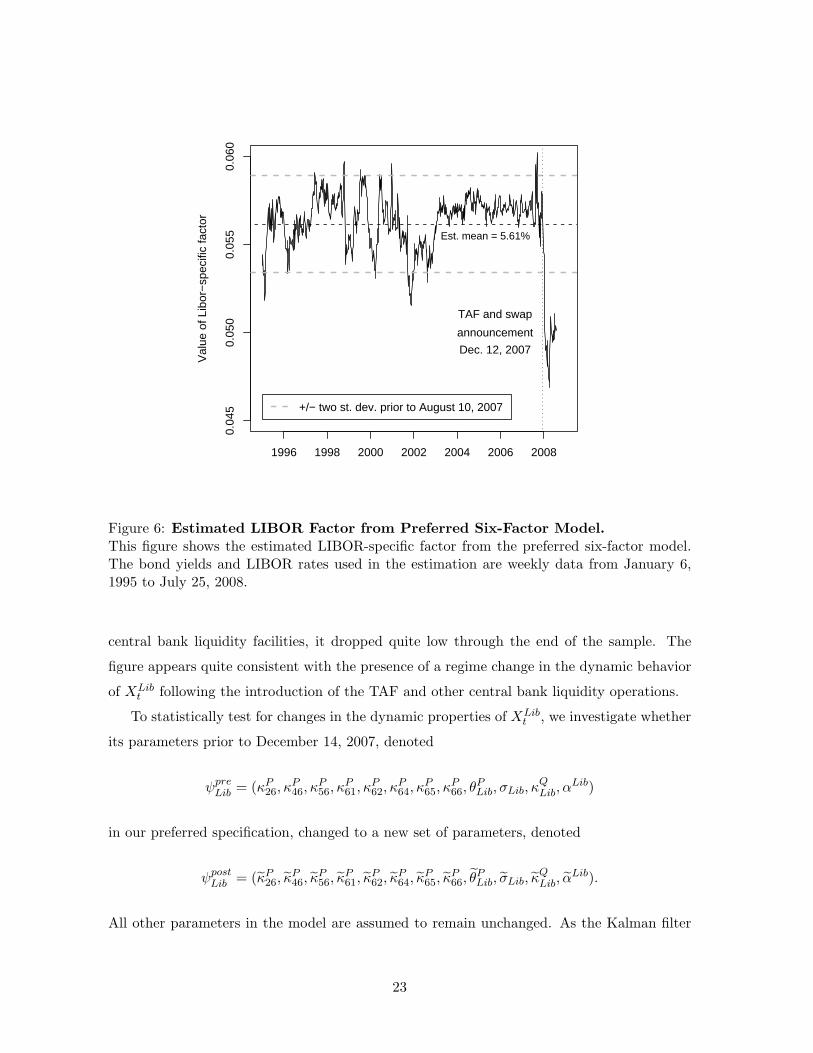
and Wang 2008, and Wu 2009). We investigate this question with our estimated model.

Figure 6 shows the estimated path of our sixth factor, which is specific to the LIBOR market.

Deviations of this factor from its mean (shown by a horizontal dashed line) indicate the

direction and approximate size of the difference between the yield on AA-rated U.S. financial

bonds and term LIBOR rates of the same maturity. Until December 2007, this factor moved

within a fairly close range around its mean. However, following the introduction of the

22

1996 1998 2000 2002 2004 2006 2008

0.04

50.

050

0.05

50.

060

Val

ue o

f Lib

or−

spec

ific

fact

or

Est. mean = 5.61%

TAF and swap

announcement

Dec. 12, 2007

+/− two st. dev. prior to August 10, 2007

Figure 6: Estimated LIBOR Factor from Preferred Six-Factor Model.This figure shows the estimated LIBOR-specific factor from the preferred six-factor model.The bond yields and LIBOR rates used in the estimation are weekly data from January 6,1995 to July 25, 2008.

central bank liquidity facilities, it dropped quite low through the end of the sample. The

figure appears quite consistent with the presence of a regime change in the dynamic behavior

of XLibt following the introduction of the TAF and other central bank liquidity operations.

To statistically test for changes in the dynamic properties of XLibt , we investigate whether

its parameters prior to December 14, 2007, denoted

ψpreLib = (κP

26, κP46, κ

P56, κ

P61, κ

P62, κ

P64, κ

P65, κ

P66, θ

PLib, σLib, κ

QLib, α

Lib)

in our preferred specification, changed to a new set of parameters, denoted

ψpostLib = (κP

26, κP46, κ

P56, κ

P61, κ

P62, κ

P64, κ

P65, κ

P66, θ

PLib, σLib, κ

QLib, α

Lib).

All other parameters in the model are assumed to remain unchanged. As the Kalman filter

23

KP KP·,1 KP

·,2 KP·,3 KP

·,4 KP·,5 θP Σ

KP1,· -1.072 -1.208 0 0 0 0.01132 0.001884

(0.165) (0.209) (0.0275) (0.000116)KP

2,· 0.8645 0.5975 0 0 0.1343 -0.007720 0.002026(0.372) (0.396) (0.0580) (0.0239) (0.000191)

KP3,· 0 0 0.0002158 0 0 0.07634 0.004784

(0.0995) (0.120) (0.000127)KP

4,· 0 0 1.034 0.9684 -1.179 -0.03393 0.008224(0.528) (0.199) (0.187) (0.0803) (0.000247)

KP5,· 0 0 0 0 0.8492 -0.01265 0.02641

(0.547) (0.0525) (0.000656)

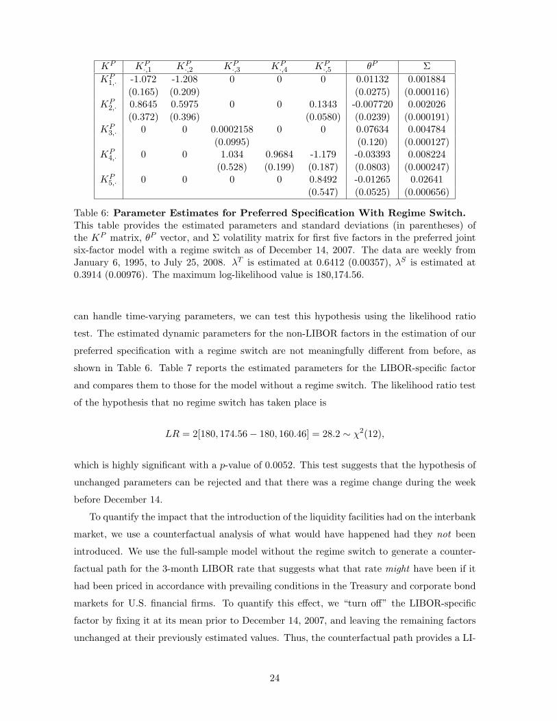
Table 6: Parameter Estimates for Preferred Specification With Regime Switch.This table provides the estimated parameters and standard deviations (in parentheses) ofthe KP matrix, θP vector, and Σ volatility matrix for first five factors in the preferred jointsix-factor model with a regime switch as of December 14, 2007. The data are weekly fromJanuary 6, 1995, to July 25, 2008. λT is estimated at 0.6412 (0.00357), λS is estimated at0.3914 (0.00976). The maximum log-likelihood value is 180,174.56.

can handle time-varying parameters, we can test this hypothesis using the likelihood ratio

test. The estimated dynamic parameters for the non-LIBOR factors in the estimation of our

preferred specification with a regime switch are not meaningfully different from before, as

shown in Table 6. Table 7 reports the estimated parameters for the LIBOR-specific factor

and compares them to those for the model without a regime switch. The likelihood ratio test

of the hypothesis that no regime switch has taken place is

LR = 2[180, 174.56− 180, 160.46] = 28.2 ∼ χ2(12),

which is highly significant with a p-value of 0.0052. This test suggests that the hypothesis of

unchanged parameters can be rejected and that there was a regime change during the week

before December 14.

To quantify the impact that the introduction of the liquidity facilities had on the interbank

market, we use a counterfactual analysis of what would have happened had they not been

introduced. We use the full-sample model without the regime switch to generate a counter-

factual path for the 3-month LIBOR rate that suggests what that rate might have been if it

had been priced in accordance with prevailing conditions in the Treasury and corporate bond

markets for U.S. financial firms. To quantify this effect, we “turn off” the LIBOR-specific

factor by fixing it at its mean prior to December 14, 2007, and leaving the remaining factors

unchanged at their previously estimated values. Thus, the counterfactual path provides a LI-

24

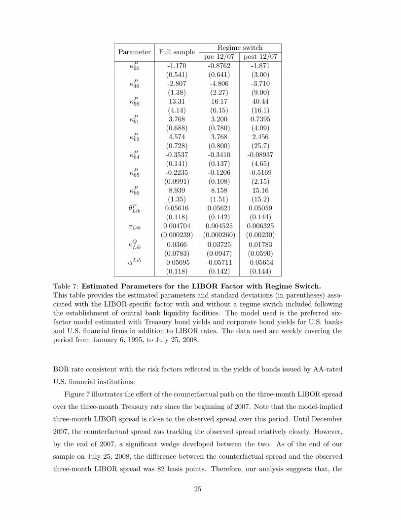
Regime switchParameter Full samplepre 12/07 post 12/07

κP26 -1.170 -0.8762 -1.871

(0.541) (0.641) (3.00)κP

46 -2.807 -4.806 -3.710(1.38) (2.27) (9.00)

κP56 13.31 16.17 40.44

(4.14) (6.15) (16.1)κP

61 3.768 3.200 0.7395(0.688) (0.780) (4.09)

κP62 4.574 3.768 2.456

(0.728) (0.800) (25.7)κP

64 -0.3537 -0.3410 -0.08937(0.141) (0.137) (4.65)

κP65 -0.2235 -0.1206 -0.5169

(0.0991) (0.108) (2.15)κP

66 8.939 8.158 15.16(1.35) (1.51) (15.2)

θPLib 0.05616 0.05621 0.05059

(0.118) (0.142) (0.144)σLib 0.004704 0.004525 0.006325

(0.000239) (0.000260) (0.00230)κQ

Lib 0.0366 0.03725 0.01783(0.0783) (0.0947) (0.0590)

αLib -0.05695 -0.05711 -0.05654(0.118) (0.142) (0.144)

Table 7: Estimated Parameters for the LIBOR Factor with Regime Switch.This table provides the estimated parameters and standard deviations (in parentheses) asso-ciated with the LIBOR-specific factor with and without a regime switch included followingthe establishment of central bank liquidity facilities. The model used is the preferred six-factor model estimated with Treasury bond yields and corporate bond yields for U.S. banksand U.S. financial firms in addition to LIBOR rates. The data used are weekly covering theperiod from January 6, 1995, to July 25, 2008.

BOR rate consistent with the risk factors reflected in the yields of bonds issued by AA-rated

U.S. financial institutions.

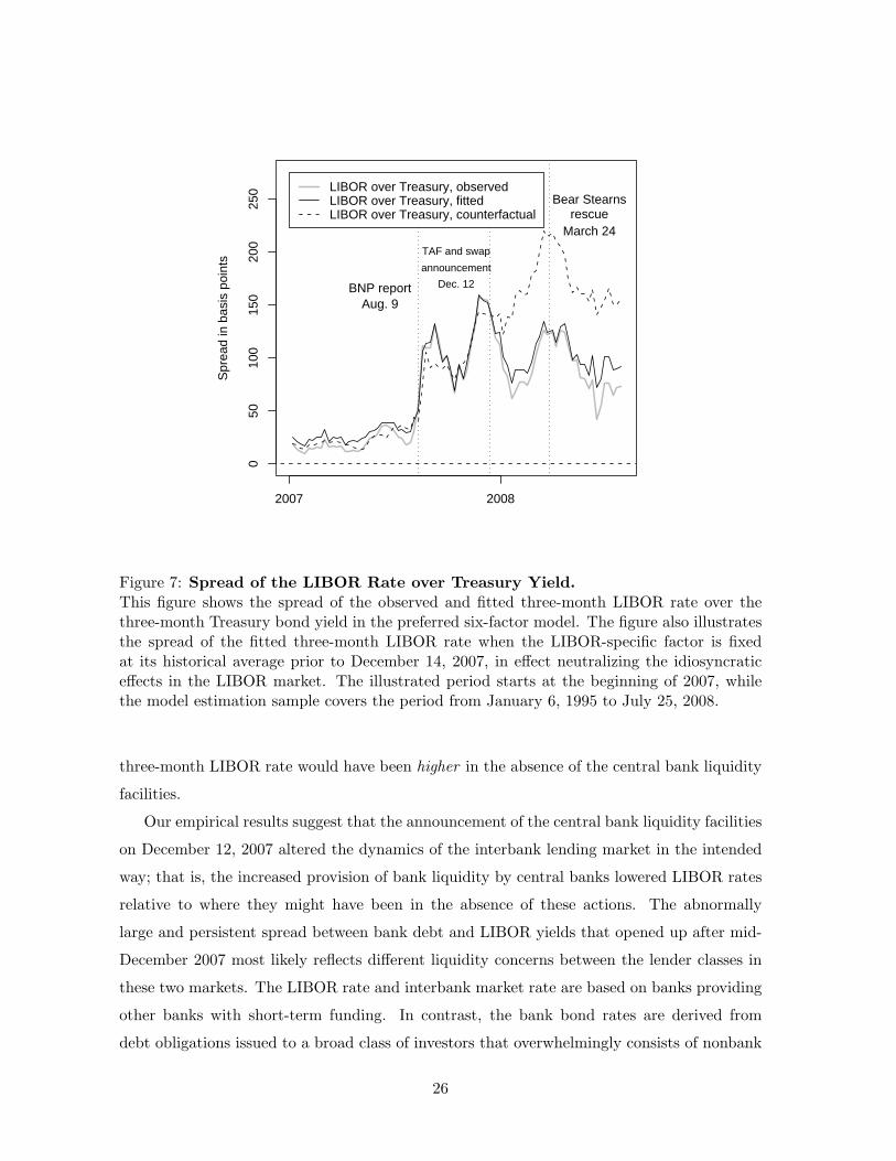
Figure 7 illustrates the effect of the counterfactual path on the three-month LIBOR spread

over the three-month Treasury rate since the beginning of 2007. Note that the model-implied

three-month LIBOR spread is close to the observed spread over this period. Until December

2007, the counterfactual spread was tracking the observed spread relatively closely. However,

by the end of 2007, a significant wedge developed between the two. As of the end of our

sample on July 25, 2008, the difference between the counterfactual spread and the observed

three-month LIBOR spread was 82 basis points. Therefore, our analysis suggests that, the

25

2007 2008

050

100

150

200

250

Spr

ead

in b

asis

poi

nts

BNP reportAug. 9

TAF and swap

announcement

Dec. 12

Bear Stearnsrescue

March 24

LIBOR over Treasury, observed LIBOR over Treasury, fitted LIBOR over Treasury, counterfactual

Figure 7: Spread of the LIBOR Rate over Treasury Yield.This figure shows the spread of the observed and fitted three-month LIBOR rate over thethree-month Treasury bond yield in the preferred six-factor model. The figure also illustratesthe spread of the fitted three-month LIBOR rate when the LIBOR-specific factor is fixedat its historical average prior to December 14, 2007, in effect neutralizing the idiosyncraticeffects in the LIBOR market. The illustrated period starts at the beginning of 2007, whilethe model estimation sample covers the period from January 6, 1995 to July 25, 2008.

three-month LIBOR rate would have been higher in the absence of the central bank liquidity

facilities.

Our empirical results suggest that the announcement of the central bank liquidity facilities

on December 12, 2007 altered the dynamics of the interbank lending market in the intended

way; that is, the increased provision of bank liquidity by central banks lowered LIBOR rates

relative to where they might have been in the absence of these actions. The abnormally

large and persistent spread between bank debt and LIBOR yields that opened up after mid-

December 2007 most likely reflects different liquidity concerns between the lender classes in

these two markets. The LIBOR rate and interbank market rate are based on banks providing

other banks with short-term funding. In contrast, the bank bond rates are derived from

debt obligations issued to a broad class of investors that overwhelmingly consists of nonbank

26

institutions. While these two classes of lenders most likely attach similar probabilities and

prices to credit risk, they likely have different tolerances to liquidity problems. The different

degrees to which central bank liquidity operations lowered the liquidity concerns of lenders

in the interbank market by more than those in the bank bond market would be translated

directly into the spread between these two markets. (Appendix 2 provides a simple conceptual

framework that illustrates this effect.)

There are two other explanations that could also account for the increased spread be-

tween bank debt yields and LIBOR rates, but these alternatives do not convincingly fit this

episode. The first explanation centers on changes in the nature or the quality of the data.

In mid-April 2008, there were news reports that the 16 banks surveyed as part of the daily

fixing of the LIBOR rates on U.S. dollar-denominated term deposits were underreporting

their actual borrowing costs. If such underreporting were new, the distress in the interbank

market would be more severe than reflected in LIBOR rates, and those rates would be low

relative to the bank bond yields. However, the persistence of the high LIBOR spread through

the end of our sample period despite a speedy investigation and resolution of these underre-

porting accusations seems to undermine this possible explanation. Alternatively, the quality

of the corporate bond data, especially since August 2007, could be questioned due perhaps to

reduced bond trading. Yet, the persistence of the larger spread over several months weakens

this possible explanation as well. Also, it is hard to see why these data considerations would

be linked to a mid-December regime shift.

The second alternative explanation for the larger spread is the possibility of a change in the

relative credit risk characteristics of the bank debt and interbank loan markets, for example,

through changes in perceived recovery rates.23 Again, during our sample—and notably even

during the 2001 recession—there were no substantial similar differences in relative credit

risk. Furthermore, it is difficult to date any changes a priori to mid-December 2007. Still,

conceivably, changes could have occurred in the relative credit risk between the LIBOR panel

of international AA-rated banks and the domestic AA-rated banks and financial firms used to

construct the Bloomberg bank debt curves. To examine this possibility within the context of

our model, we generated synthetic five-year credit default swap (CDS) rates for the AA-rated

U.S. financial firms and compared these to the median five-year CDS rate for the banks in the23An unsecured deposit (e.g., an interbank loan) is more senior in the liability structure of a bank than

senior unsecured debt. McAndrews, Sarkar, and Wang (2008) mention a recovery rate of 91.25% for unsecureddeposits at banks with assets larger than $5 billion, as per the work of Kuritzkes, Schuermann, and Weiner(2005). On the other hand, the data provider Markit typically works with a recovery rate as low as 40% in itspricing of credit default swap contracts. However, it is not clear why this difference in recovery rates wouldhave changed dramatically in December 2007.

27

2007 2008

050

100

150

200

Rat

e

Model−implied 5−yr CDS rate, AA financials Median 5−yr CDS rate, LIBOR banks

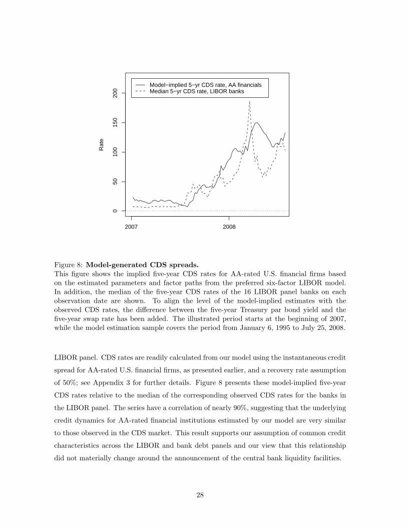
Figure 8: Model-generated CDS spreads.This figure shows the implied five-year CDS rates for AA-rated U.S. financial firms basedon the estimated parameters and factor paths from the preferred six-factor LIBOR model.In addition, the median of the five-year CDS rates of the 16 LIBOR panel banks on eachobservation date are shown. To align the level of the model-implied estimates with theobserved CDS rates, the difference between the five-year Treasury par bond yield and thefive-year swap rate has been added. The illustrated period starts at the beginning of 2007,while the model estimation sample covers the period from January 6, 1995 to July 25, 2008.

LIBOR panel. CDS rates are readily calculated from our model using the instantaneous credit

spread for AA-rated U.S. financial firms, as presented earlier, and a recovery rate assumption

of 50%; see Appendix 3 for further details. Figure 8 presents these model-implied five-year

CDS rates relative to the median of the corresponding observed CDS rates for the banks in

the LIBOR panel. The series have a correlation of nearly 90%, suggesting that the underlying

credit dynamics for AA-rated financial institutions estimated by our model are very similar

to those observed in the CDS market. This result supports our assumption of common credit

characteristics across the LIBOR and bank debt panels and our view that this relationship

did not materially change around the announcement of the central bank liquidity facilities.

28

5 Conclusion

In this paper, we address the question of whether interbank lending rates have responded to

central bank liquidity operations by using a six-factor AFNS model that encompasses Treasury

yields, financial corporate debt yields, and LIBOR rates. Our results provide support for the

view that these operations, such as the introduction of the TAF, did lower LIBOR rates

starting in December 2007 and through the end of our sample in July 2008. We find that the

parameters governing the LIBOR factor in our model appear to change after the introduction

of the liquidity facilities; i.e., the hypothesis of constant parameters over the full sample

period is rejected. This result suggests that the behavior of this factor, and thus of the

LIBOR market, was directly affected by these central bank liquidity operations. To quantify

this effect, we use the model to construct a counterfactual path for the three-month LIBOR

rate. The counterfactual three-month LIBOR rate averaged significantly higher than the

observed rate from December 2007 into midyear 2008, which suggests that if the central bank

liquidity operations had not occurred, the three-month LIBOR spread over Treasuries would

have been even higher than the observed historical spread.

29

Appendix 1: Conversion of interest rate data

We convert the Bloomberg data for financial corporate bond rates into continuously com-

pounded yields. The n-year yield at time t, rt(n), the corresponding zero-coupon bond price,

Pt(n), and the continuously compounded yield, yt(n), are related by

Pt(n) =1

(1 + rt(n))n= e−yt(n)n ⇐⇒ yt(n) = − 1

nln

1(1 + rt(n))n

= ln(1 + rt(n)).

For maturities shorter than one year, we assume the standard convention of linear interest

rates. For example, the zero-coupon bond price corresponding to the six-month yield is

calculated as

Pt(6m) =1

1 + 0.5rt(6m)= e−0.5yt(6m),

and the corresponding continuously compounded yield as

yt(6m) = −2 ln1

1 + 0.5rt(6m)= 2 ln(1 + 0.5rt(6m)).

We also convert the LIBOR rates into continuously compounded yields, as in Feldhutter

and Lando (2008). To facilitate this conversion, we approximate the day count ratio assuming

that the LIBOR curve is smooth. Therefore, the net present value of the three-month LIBOR

contract is

NPV Libt =

11 + 1

4L(t, t + 0.25)= e−0.25yLib(t,t+0.25),

where L(t, t + 0.25) denotes the quoted three-month LIBOR rate. The continuously com-

pounded equivalent to the quoted three-month LIBOR rates is then

yLib(t, t + 0.25) = −4 log[ 11 + 1

4L(t, t + 0.25)

]= 4 log(1 + 0.25L(t, t + 0.25)).

Similarly, the six-month and twelve-month LIBOR rates can be converted into continuously

compounded zero-coupon yields by the following formulas:

yLib(t, t + 0.5) = 2 log(1 + 0.5L(t, t + 0.5)),

yLib(t, t + 1) = log(1 + L(t, t + 1)).

30

Appendix 2: Conceptual framework to illustrate liquidity risk effects

To help interpret the relative movements in Treasury, bank bond, and interbank rates and

to motivate our empirical analysis, we present a very simple framework to illustrate differential

credit and liquidity risks across different debt obligations and, by extension, how the provision

of central bank liquidity can have differential effects on their associated yields. We assume a

simple three-period setting in which at date zero, lenders must choose among three different

2-period securities as to where to invest their funds. The first investment option is a liquid

Treasury security, which pays the risk-free rate of interest, which we normalize to zero, so

a dollar invested in the liquid asset at date zero returns a dollar at date two. The second

investment option is a bank-issued bond, in which a dollar invested at date zero will return

1 + rB dollars at date two. The third investment option is an interbank loan, which will

return 1 + rL dollars at date two for a dollar invested at time zero. The rates of return, rB

and rL, will be positive to account for credit and liquidity risk.

We assume that the markets for bank bonds and interbank loans are segmented to some

degree, with differing market microstructures and lender preferences; in which case, rB is not

always identical to rL, which is consistent with the observed data. Specifically, the interbank

market investors are predominantly banks providing other banks with short-term funding.

In contrast, bank bonds are issued to a much broader class of investors that overwhelmingly

consists of nonbank institutions. We assume these two classes of lenders share the same

perception of and attach the same price to credit risk. However, regarding liquidity risk, we

assume that the two classes of lenders may face different liquidity shocks during the term

of the debt at date one and may price that liquidity risk differently. Formally, we assume

that at date one, bank bond investors are subject to a liquidity shock, such as an unexpected

demand for funds, that induces an adjustment cost of αB1 with a probability λB

1 . In addition,

the interbank lenders are subject to a liquidity shock that induces an adjustment cost of

αL1 with a probability λL

1 . Investors in Treasuries can costlessly satisfy any liquidity shocks.

Furthermore, at date two, the two bank investment options are also subject to a common

default event, in which the borrowing bank declares insolvency, with probability λ2 and cost

δ, which is less than one to reflect only partial repayment of the principal. Any such partial

recovery is shared equally by bondholders and interbank creditors.

Given this structure, the rate of return on the Treasury bond at date zero for date two

is zero. Assuming that bond investors are indifferent between bank and Treasury bonds and

that interbank lenders are indifferent between the Treasury bond and the interbank loan, the

31

expected returns on the illiquid assets are:

rB = λB1 αB

1 + λ2δ and rL = λL1 αL

1 + λ2δ.

That is, the returns compensate for the costs associated with the date-one liquidity shocks

and the date-two default, as weighted by the respective probabilities. Note that rB and rL,

and their corresponding spreads over the Treasury rate, will move together with changes in

the borrowing bank’s default risk, so the jumps in the spread of LIBOR over the Treasury

rate can reflect both credit and liquidity risk.

In contrast, in our simple theoretical structure, the spread between the bank bond rate

and the LIBOR rate only reflects liquidity risk:

rB − rL = λB1 αB

1 − λL1 αL

1 .

Therefore, fluctuations in counterparty risk will not affect this spread, which in our data

is the spread of the AA-rated bank debt yield over the corresponding LIBOR rate. In the

early stage of the crisis, the spread was negative as the LIBOR rate rose relative to the bank

debt rates. In our framework, this outcome would suggest that λL1 αL

1 , the liquidity risk for

interbank lenders, initially rose during the financial turmoil relative to the corresponding cost

for the bank bond investors. The spread remained negative until roughly mid-December when

the Federal Reserve and other central banks announced liquidity operations concentrating on

the interbank market. After that, LIBOR declined sharply relative to the corresponding bank

debt rates, and the spread rose. Again, our framework suggests that the central bank liquidity

operations lowered the illiquidity cost and probability parameters for banks.

32

Appendix 3: The swap premium of a plain vanilla CDS

In this appendix, the reduced-form pricing of credit default swaps is described. It is

assumed that there is a model for the instantaneous risk-free interest rate rt, a model for the

default intensity of the representative firm considered λt, and a model for the loss rate given

default Lt. Let T denote the time to maturity of the CDS contract and let t1, . . . , tN denote

the swap premium payment dates. In case of default before T , the payment on the default

leg is assumed to be the loss rate Lt times the size of the notional. Given these assumptions

the value of the default leg of a plain vanilla CDS contract per $1 notional can be calculated

as

V CDSdef (0, T ) = EQ

[ ∫ T

0Ls1{s<τ≤s+ds}e−

∫ s0 rududs

∣∣∣F0

]

= EQ[ ∫ T

0Lsλse

− ∫ s0 (ru+λu)duds

∣∣∣F0

],

where τ is the unpredictable time of the first jump of the point process which indicates the

default time in reduced-form credit risk models (for details see Lando, 1998).

In return for the loss protection, the protection buyer has to pay a premium, here denoted

by SCDS(0, T ) and quoted at an annual rate. If we define δi = ti−ti−1 to be the time between

the ith and the (i-1)th payment dates, the contractual payment on the ith payment date equals

δiSCDS(0, T ). In addition, the market convention requires the accrued swap premium since

the last payment date to be paid immediately upon default in exchange for the default leg

payment. Given this convention, the value of the premium leg can be calculated as

V CDSprem (0, T ) = EQ

[SCDS(0, T )

N∑

i=1

δi1{τ>ti}e− ∫ ti

0 rudu|F0

]

+ EQ[ N∑

i=1

∫ ti

ti−1

SCDS(0, T )(s− ti−1)1{s<τ≤s+ds}e−∫ s0 rududs|F0

]

= SCDS(0, T )EQ[ N∑

i=1

δie− ∫ ti

0 (ru+λu)du +N∑

i=1

∫ ti

ti−1

(s− ti−1)λse− ∫ s

0 (ru+λu)duds|F0

].

At inception, the swap premium is set to give the contract a value of zero:

SCDS(0, T ) =EQ

[ ∫ T0 Lsλse

− ∫ s0 (ru+λu)duds|F0

]

EQ[∑N

i=1 δie−∫ ti0 (ru+λu)du +

∑Ni=1

∫ titi−1

(s− ti−1)λse− ∫ s

0 (ru+λu)duds|F0

] .

33

In the six-factor LIBOR model, the instantaneous risk-free rate is given by

rt = LTt + ST

t ,

while the instantaneous credit spread of the representative AA-rated U.S. financial firm, which

is the category we map to LIBOR, is given by

sAA,F int = αAA,F in

0 + αAA,F inLT LT

t + αAA,F inST ST

t + αAA,F inLS LS

t + αAA,F inSS SS

t .

If we fix the expected loss rate at L = 50%, which is an assumption frequently made in

the credit risk literature, we can solve for the default intensity process consistent with the

estimated instantaneous credit spread process of the representative AA-rated U.S. financial

firm by using the following no-arbitrage restriction that must hold for the instantaneous credit

spread

sAA,F int = LλAA,F in

t ⇒ λAA,F int =

1L

sAA,F int .

With the assumption of L = 50%, this translates into

λAA,F int = 2αAA,F in

0 + 2αAA,F inLT LT

t + 2αAA,F inST ST

t + 2αAA,F inLS LS

t + 2αAA,F inSS SS

t .

Combining the Q-dynamics of the AFNS state variables with the general asset pricing result

for affine models provided in Duffie, Pan, and Singleton (2000), CDS rates for the represen-

tative AA-rated U.S. financial firm can be calculated by solving straightforward systems of

ordinary differential equations.

34

References

Allen, Franklin, Elena Carletti, and Douglas Gale, 2009, “Interbank Market Liquidity and

Central Bank Intervention,” Working paper #2009-12, Wharton Financial Institutions

Center.

Christensen, Jens H. E., Francis X. Diebold, and Glenn D. Rudebusch, 2007, “The Affine

Arbitrage-free Class of Nelson-Siegel Term Structure Models,” unpublished working

paper, Federal Reserve Bank of San Francisco.

Christensen, Jens H. E., and Jose A. Lopez, 2008, “Common Risk Factors in the U.S. Trea-

sury and Corporate Bond Markets: An Arbitrage-free Dynamic Nelson-Siegel Modeling

Approach,” unpublished working paper, Federal Reserve Bank of San Francisco.

Christensen, Jens H. E., Jose A. Lopez, and Glenn D. Rudebusch, 2008, “Inflation expecta-

tions and risk premiums in an arbitrage-free model of nominal and real bond yields,”

Working Paper Series 2008-34, Federal Reserve Bank of San Francisco.

Collin-Dufresne, Pierre, and B. Solnik, 2001, “On the Term Structure of Default Premia in

the Swap and LIBOR Markets,” Journal of Finance, 56, 1095-1115.

Driessen, Joost, 2005, “Is Default Event Risk Priced in Corporate Bonds?,” Review of

Financial Studies, 18, 165-195.

Duffee, Gregory R., 2008, “Forecasting with the Term Structure: The Role of No-Arbitrage,”

manuscript, Johns Hopkins University.

Duffie, Darrell, and Rui Kan, 1996, “A Yield-Factor Model of Interest Rates,” Mathematical

Finance, 6, 379-406.

Duffie, Darrell, Jun Pan, and Kenneth Singleton, 2000, ”Transform Analysis and Asset

Pricing for Affine Jump Diffusions,” Econometrica 68, 1343-1376.

Federal Reserve Board of Governors, Press release. December 12, 2007.

Feldhutter, Peter, and David Lando, 2008, “Decomposing Swap Spreads,” Journal of Finan-

cial Economics, 88, 375405.

Gurkaynak, Refet S., Brian Sack, and Jonathan H. Wright, 2007, “The U.S. Treasury Yield

Curve: 1961 to the Present,” Journal of Monetary Economics, 54, 2291-2304.

35

Kim, Don H., and Athanasios Orphanides, 2005, “Term Structure Estimation with Survey

Data on Interest Rate Forecasts,” Finance and Economics Discussion Series, 2005-48,

Board of Governors of the Federal Reserve System.

Kuritzkes, Andrew, Til Schuermann, and Scott M. Weiner, 2005, “Deposit Insurance and

Risk Management of the U.S. Banking System: What is the Loss Distribution Faced by

the FDIC?,” Journal of Financial Services Research, 27, 217-242.

Lando, David, 1998, “On Cox Processes and Credit Risky Securities,” Review of Derivatives

Research, vol. 2, 99-120.

Li, Haitao, Junbo Wang, Chunchi Wu, and Yan He, 2009, “Are Liquidity and Information

Risks Priced in the Treasury Bond Market?” Journal of Finance, 64, 467-503.

Litterman, R., and J. A. Scheinkman, 1991, “Common Factors Affecting Bond Returns,”

Journal of Fixed Income, 1, 62-74.

McAndrews, James, Asani Sarkar, and Zhenyu Wang, 2008, “The Effect of the Term Auction

Facility on the London Inter-Bank Offered Rate,” Staff Report No. 335, Federal Reserve

bank of New York.

Neely, C.J. and Winters, D.B., 2006, “Year-End Seasonality in One-Month LIBOR Deriva-

tives,” Journal of Derivatives, 13(3), 47-65.

Nelson, Charles R., and Andrew F. Siegel, 1987, “Parsimonious Modeling of Yield Curves,”

Journal of Business, 60, 473-489.

Taylor, John B., and John C. Williams, 2009, “A Black Swan in the Money Market,” Amer-

ican Economic Journal: Macroeconomics, 1(1): 58-83.

Wu, Tao, 2009, “The U.S. Money Market and the Term Auction Facility in Financial Crisis

of 2007-2009,” unpublished working paper, Federal Reserve Bank of Dallas.

36