How demand analysis can help improve fisheries and

Sean Pascoe, Peggy Schrobback and Eriko HoshinoFRDC Project No 2018-017 | February 2021

How demand analysis can help improve fisheries and aquaculture performance

How demand analysis can help improve fisheries and aquaculture performance CSIRO Australia’s National Science Agency2

Contents

Introduction 3

Key concepts and terminology 4

What factors affect seafood price? 4

“Demand curves” and the relationship between price and quantity 6

Price elasticity versus price flexibility 6

Examples of price flexibilities for seafood in Australian markets 7

What affects own-price flexibility? 8

Market interactions between species and substitute goods 9

Market dynamics – short run and long run price flexibilities 10

Implications of price flexibilities for fisheries and aquaculture management 11

Price flexibility, revenues and profits 11

Unanticipated effects of TAC and aquaculture production changes 13

Changes in trade: imports and exports 13

Price flexibility and benefits to consumers 14

Conclusions 15

Appendix: Estimated short and long run price flexibilities 16

Fish species 16

Prawns 17

Oysters 18

References 19


IntroductionAs it is currently applied in Australia, fisheries management is mainly focused on ensuring the sustainability of the resource while maximising the output from the fishery. This is largely achieved through setting total allowable catch (TAC) or equivalent effort restrictions to limit the quantity of landings from the fishery. In jurisdictions where economic outcomes are also important, more conservative catch and effort limits are generally set in recognition of the additional cost of harvesting the resource as stock size declines.

For aquaculture, while not directly subject to production limits in the same way that wild-caught fisheries are, regulation can affect output levels in other ways. For example, the number of licenced pens or the area available for oyster leases in an estuary may be restricted. Changes in these restrictions, such as through expanding the area available for aquaculture, will change the productive capacity of the sector, and subsequently change the level of output.

What happens after the catch is landed or product is harvested is generally considered a business decision of the fisher/farmer. Where they sell their catch, and how much they get for it, is not generally under the control of managers. However, how much is caught or farmed can affect the price received, and this is directly under the control of managers.

While fishers have many options (e.g. different auction markets, direct to processors or retailer, or even direct to public), the prices in all these markets are generally linked to the overall quantity of fish landed or produced. At the individual fisher/farmer level, the impact of the amount they catch or produce on the total quantity supplied to the market will often be small, and the link between their level of production and the price received may not be apparent. However, at the industry level, the quantity produced can have a substantial impact on the price all producers receive. This, in turn, is directly affected by fisheries and aquaculture management through the catch or effort limits imposed or the other restrictions placed on production.

The aim of this document is to highlight the importance of taking market effects into account when prices vary with quantity landed, and to present some key economic concepts that managers and industry can factor into decision making. The scope of the document does not include a description of how the relationship between price and quantity landed is estimated1, but aims to help mangers and industry understand the outputs of these analyses and how they may be considered in management decisions.

www.sydneyfishmarket.com.au/Seafood-Trading

1

1 These are covered in more detail in Pascoe, et al. [1].


Key concepts and terminology The analysis of the relationship between quantity and price, known as demand analysis, involves several key concepts and terms which may appear jargonistic. Most studies in the area have been published in academic journals, and an understanding of the terminology commonly used will be of benefit to managers and industry members trying to apply the key concepts to their decision making. In this section, some of the basic theory underpinning these analyses is presented, along with a description of the common terminology used.

What factors affect seafood price?Seafood production through fishing and aquaculture is a commercial business, and the price received for the product is as important to determining revenue as the quantity landed or produced. The relationship between quantity produced and price received is determined by the demand for the product on the markets. The analyses of these relationships is consequently known as demand analysis.

2


The price received is determined by a number of factors, many of which are beyond the control of the individual producer. The importance of these factors varies from species to species, depending on where it is sold (i.e. domestic or export market) as well as the characteristics of the individual species. However, a key factor, and one that is under the control of fisheries and aquaculture managers, is the quantity landed at an industry level (not at an individual firm level) or produced of the different species.

Changes in the quantity landed or produced of a species can also impact the prices received of other species, with this impact depending on the characteristics of the species. Characteristics in this case refers to those important to consumers (e.g. taste, firmness, size of bones, etc), not biological characteristics. Species with similar characteristics are potential substitutes, regardless of whether they are landed/produced domestically or imported.

Seasonal factors can also affect the level of demand, and subsequent price of fish and seafood. For example, prawn prices tend to increase around Christmas, New Year and Easter. Similarly, prices of exported species also tend to increase around festival periods in the countries to which they are exported.

Furthermore, changes in global production can impact on prices of Australian products if they are sold into the export market. If Australia has only a small market share on the export market, then what happens in other countries will have – potentially – a greater impact on prices received than how much is produced in Australia.

On the domestic market, increased global production is likely to result in increased imports. The increased supply of imported substitute goods can impact domestic prices of Australian produced product. The magnitude of the impact will depend on the degree of substitutability, which will vary due to the characteristics of the imports and the domestically produced species.

Changes in income can also affect the demand for seafood, impacting on its price. For example, increase in higher income population tend to increase in demand for premium seafood. These impacts can be assessed through separate modelling techniques, which are not detailed further in this overview document.

Sustainability certification by third parties (e.g. Marine Stewardship Council) is becoming increasingly important to access some markets, and in some cases has been shown to influence the price received. This can be influenced by management, as certification often requires management instruments are in place to enable fish to be harvested or produced in a sustainable manner with minimum environmental impact.

Other shocks, such as oils or chemical spills and toxic algae blooms, can impact the demand for fisheries products even beyond those directly affected by the initial problem. For example, toxic algal blooms have been found to negatively impact shellfish supplied from unaffected regions [2], while prices for fish from unaffected regions of Japan declined following the Fukushima disaster [3].

As noted above, most of these factors are beyond the control of managers. While managers need to be aware of the potential implications of changes in the market environment, the factor that they can control is the quantity landed or produced of different species.

Fishprice

3rd PartyCer�fica�on

Quan�tylanded/

produced

Quan�tysubs�tute

species

Incomelevels

Season/fes�vals

Exchangerates

(exports)Marketshare

Direct control of managers

In�uenced by management

Outside control of managers


“Demand curves” and the relationship between price and quantityIn economics, demand analysis is the study of the relationship between quantities of a good on the market and its price. There is substantial economic theory underpinning demand analysis, but the simple version is that there is an inverse relationship between price and quantity. In the case of fisheries and aquaculture, prices change with the amount landed or produced.

This is generally represented by a downward sloping demand curve. This can be considered from the perspective of both the consumer and the producer. From the consumers’ perspective, a decrease in the price will lead to more of the product being bought. From the producers’ perspective, lower prices result in more product being sold. In the case of fisheries and aquaculture producers, who are generally price takers and unable to influence the price received directly, the price they receive will depend on the total supply to the market and the strength of the price-quantity relationship (i.e. the slope of the demand curve).

Price elasticity versus price flexibilityEconomics has two related measures of the relationship between price to quantity. From the consumers’ perspective, price is a given (i.e. in the supermarket), and is a key factor in the decision of how much to buy (if any). The change in quantity bought as price changes determines the price elasticity of the good. Price elasticity represents the percentage change in quantity demanded due to a 1 per cent change in the price. For example, for a good with a price elasticity of -2, a 1% reduction in the price of the good will result in a 2% increase in quantity demanded.

In contrast, fishers and aquaculturalists are largely price takers. Their product is highly perishable, and once on the market, must be sold. In these cases, the market price adjusts to clear the available supply. Of relevance to producers is the price flexibility – the percentage change in price due to a 1% change in quantity supplied to the market. For example, for a fish species with a price flexibility of -2, a 1% increase in the quantity landed will result in a 2% decrease in price received.

Understanding the distinction between price elasticity and price flexibility is important, as some studies focus on one measure and other studies on the other. Both price elasticities and price flexibilities are always negative. A good with a price elasticity less than -1 (e.g. -2), the demand for the good is said to be price elastic, while a price elasticity greater than -1 (e.g. -0.5), demand is price inelastic. Conversely, a product with a price flexibility less than -1 (e.g. -2) is said to be price flexible, while a price flexibility greater than -1 (e.g. -0.5) is price inflexible.

Price ($/kg)

Quan�ty (kg/period)

Increasein quan�ty

Decreasein price

Demand Curve


There is an inverse relationship between price elasticity and price flexibility. A good that is price elastic (from the consumer perspective) is price inflexible (from the producer perspective).

Examples of price flexibilities for seafood in Australian marketsFrom the perspective of fishers and aquaculture producers, of key relevance is the price flexibility of their product. Fish supplied to the market is highly perishable, and must be sold. The price adjusts to clear the market. Own- price flexibility reflects the percentage change in price of a species due to a 1% change in the quantity landed (or produced) of that species.

Several recent studies which focus on demand analysis of Australian seafood products have estimated own-price flexibilities for key fish species on the Sydney Fish Market [1], salmon [1], prawns [4] and oysters [5] (Table 1).

Fish species were generally found to be relatively price inflexible, such that a change in quantity landed/produced results in a less than proportional change in price. Further details on price flexibilities of individual fish species are given in the Appendix.

Table 1. Own-price flexibilities from recent Australian studies

Wild caught species Own-price flexibility Aquaculture species Own-price flexibility

High valued fish species -0.350 Salmon -0.652

Low valued fish species -0.519 Prawns -0.483

Prawns -0.996 Sydney Rock Oysters -1.359

Pacific Oysters -0.353

Wild caught prawns sold domestically were found to be almost unit flexible (i.e. price flexibility is about -1). This suggests that prices on the market decrease proportionally with changes in quantity landed. Farmed prawns, however, were relatively price inflexible. This most likely reflects their small market share, as a change in quantity produced has only a small impact on the total supplies to the market, and hence only a small price response, all else being equal.

Sydney rock oysters were found to be price flexible, such that a change in the quantity supplied has a greater than proportional impact on prices received (Table 1). That is, increasing the supply of Sydney Rock Oysters to the market results in a greater than proportional decrease in the price received by producers. In contrast, Pacific oysters were price inflexible.

Price ($/kg)

Price ($/kg)

Quan�ty (kg/period) Quan�ty (kg/period)

Rela�vely elas�c demand;Price inflexible.Increase in quan�ty results in a less than propor�onal decrease in price

Rela�vely elas�c demand;Price flexible.

Increase in quan�ty results in a greater

than propor�onal decrease in price


What affects own-price flexibility?Price flexibility is affected by a number of factors, including the number of substitutes available and the share of the product in the total market. While not fisheries examples, the demand for fuel and tobacco is highly inelastic due to the lack of substitutes, hence efforts by consortiums such as OPEC to restrict oil supply to maintain high fuel prices and high taxes on tobacco to try and reduce its consumption.

Individual fish species have many potential substitutes (i.e. other fish species or even other protein sources). As a result, fish species generally have price flexibilities greater than -1 (i.e. between -1 and zero). Other seafood products, such as prawns and oysters, are not as substitutable as they are less of a staple food and eaten more on special occasions. A larger proportional reduction in price is needed to attract consumers to buy more than they would normally than, say, for fish. As a result, their price flexibilities are higher.

Market share is also an important determinant of own-price flexibility. For exported fish products, where Australia is only a small contributor to the global market, prices are driven by the total global supply rather than how much is landed domestically. That is, own-price flexibility relating to Australian production may be zero (perfectly inflexible; demand perfectly elastic), and prices received may be totally independent of the quantity of product landed. However, at the global level, prices are likely to be more flexible. Hence, prices may move with changes in total global supplies, and these changes are subsequently imposed on the Australian product irrespective of its own production level.

An example of this latter effect is evident on the prices received by Australian prawn producers exporting to the global market. Over recent decades, prices received by Australian exporters have decreased by more than 50% in real terms due to increased global supplies, even though Australian production has not changed substantially other than through year to year fluctuations due to environmental factors.


Market interactions between species and substitute goodsCross-price elasticity reflects the change in quantity demanded of a good due to a change in the price of a substitute or complementary good. For example, if chicken was a substitute for fish, then a reduction in the price of chicken would be expected to result in an increase in the quantity of chicken demanded, and a subsequent reduction in the quantity of fish demanded. From the perspective of the fish producer, an increase of the supply of chicken to the market results in a reduction in the price they receive in order to sell their product. Consequently, the cross-price flexibility will also be negative in the case of a substitute product (and positive in the case of a complementary good).

The above example was hypothetical to illustrate the concepts of cross-price flexibilities and substitution effects. Most fisheries related demand studies internationally have focused on the potential substitution between different species, or their origin, and the effect of this on price formation.

The most obvious substitute for one fish species is another fish species. Different species have different characteristics (e.g. taste, firmness, size etc) so substitution is not universal. But species with similar characteristics are likely to attract similar prices, and changes in their quantity landed is likely to impact not only their own price but also of the price of the similar species. This substitution effect can apply not just to other domestically produced species, but also imports.

Examples of cross-price flexibilities between species on the NSW market, derived from [1], are shown in Table 2. These impacts are not necessarily symmetrical. For example, changes in the quantity landed of fish species into NSW has little impact on salmon prices, but changes in the quantity of salmon sent to the NSW market has a substantial impact on the price of the wild-caught fish. Similarly, quantities of wild caught fish landed has little impact on import prices, but the level of imports – particularly fresh imports – has an impact on the price of low value fish species, and to a much lesser extent high valued fish species. The relationship between the wild-caught fish species themselves is also not symmetrical; changes in the quantity landed of high value fish species has a larger (negative) impact on the price of low value species than the converse.

Table 2. Cross-price flexibilities for fish species on the NSW market

Prices of:Changes in the quantity of:

Fresh imports Frozen imports Salmon High value fish Low value fish

Fresh imports - -0.176 -0.446 -0.051

Frozen imports - -0.172 0.040

Salmon -0.104 -0.246 - -0.051 -0.027

High value fish -0.151 -0.997 - -0.134

Low value fish -0.652 0.852 -1.209 -0.295 -


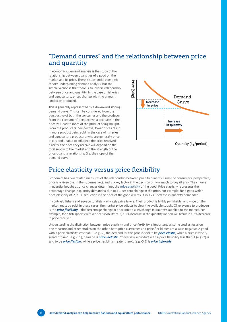
Market dynamics – short run and long run price flexibilitiesThe price flexibilities presented in the examples above are long run flexibilities. That is, they are the impact of a change in quantity on prices once a new “equilibrium” position in the market has been achieved. Markets, however, do not always react immediately to a change in landings or production, and in some instances may over-react to a change. As a result, short term price changes may be greater than, or less than, the long run price change.

The most recent estimates of short run and long run own and cross-price flexibilities for a range of key fish species, prawns and oysters are presented in the Appendix.

The short run may be fairly short: all other things being equal, for most species on the Sydney Fish Market, the long run equilibrium was achieved in 2-4 months, and for some species, nearly all price adjustment (70%) occurred in the first month [1]. The difference between the short run and long run flexibilities were also generally found to be less than +/- 10%.

Markets are also constantly subject to short term fluctuations in quantities supplied. For example, landings may vary widely on a daily or weekly basis due to the activities of the fishers as well as other factors such as weather conditions or “luck”. With the short-term dynamics noted above, prices may fluctuate widely over the year. Over the course of a fishing season, however, prices are expected to change, on average, by the degree described by the long run price flexibility.

Given the short run dynamics inherent in the price formation process as well as the constant fluctuations in landings of different species, estimation of own and cross-price flexibilities require more than a simple statistical model linking quantities landed to prices. In the case of fisheries products, estimation of dynamic inverse demand systems is generally applied, and was the basis of the estimation of the price flexibilities discussed above. Detailed descriptions of these systems are given in Pascoe, et al. [1].

Quantitychange

short run price flexibility

Short run response

long run price flexibility

Long run response


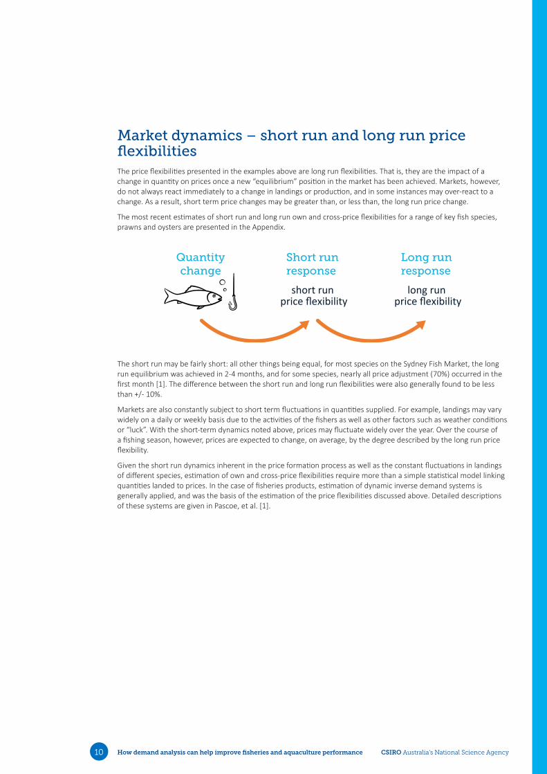
Implications of price flexibilities for fisheries and aquaculture managementPrice flexibilities provide a useful guide to managers and industry as to how revenues may change as a result of decisions that affect the quantity landed or produced. Except for the case of perfectly inflexible prices (i.e. price flexibility equals zero), an increase in output will result in a less than proportional increase in revenue as prices decline, and may even result in an overall decrease in revenue.

In this section, we present some examples as to how fishery and aquaculture economic performance may change as a result of changes in production when prices are flexible (i.e. prices change with quantity landed or produced).

Price flexibility, revenues and profitsRevenue is determined by the quantity multiplied by the price. As these both move in opposite directions (the degree to which is determined by the price flexibility), a change in quantity does not result in a proportional change in revenue. Increasing production also requires higher costs, such that profits may increase by less than any increase in quantity, and may even decrease. These effects are illustrated by some examples below.

When prices are inflexible (i.e. when demand is elastic), an increase in the quantity supplied will result in a less than proportional reduction in price (and vice versa). For example, if the quantity of fish landed increased by 10% and its price flexibility was -0.5 (i.e. price inflexible), then prices would fall by 5%. The net effect would be a 4.5% increase in revenue (i.e. 1.1 (catch) * 0.95 (price) = 1.045, as the lower price applies to the whole catch or production). Conversely, if catch or production fell by 10%, prices would increase by 5% and revenue would only fall by 5.5% (i.e. 0.9 (catch) * 1.05 (price) = 0.945).

3


Table 3. Impact of quantity change when price flexibility is -0.5 (inflexible)

Change Quantity Price Revenue

Base 1.0 1.00 1.000

Increase 10% 1.1 0.95 1.045

Decrease 10% 0.9 1.05 0.945

When prices are flexible (i.e. demand is inelastic), an increase in the quantity supplied will result in a greater than proportional reduction in prices. Using the above example, if the quantity of fish landed or produced increased by 10% and its price flexibility was -2.0 (i.e. price flexible), then prices would fall by 20%. The net effect would be a 12% decrease in revenue (i.e. 1.1 (catch) * 0.8 (price) = 0.88, as the lower price applies to the whole catch or production). Conversely, if catch or production fell by 10%, prices would increase by 20% and revenue would only increase by 8% (i.e. 0.9 (catch) * 1.2 (price) = 1.08).

Table 4. Impact of quantity change when price flexibility is -2.0 (flexible)

Change Quantity Price Revenue

Base 1.0 1.00 1.00

Increase 10% 1.1 0.80 0.88

Decrease 10% 0.9 1.20 1.08

While revenues increase less than proportionally with increased catch, costs of fishing also increase. Applying additional fishing effort to take the additional catch requires additional fuel, while higher catches also require more packaging and labour. This may result in a smaller increase in fishery profits, or potentially a decrease.

To illustrate this we present an example based on the trawl sector of the South Eastern Shark and Scalefish fishery (SESSF), using economic (cost and earnings data and price data) from ABARES [6, 7] and catch and total allowable catch (TAC) information from AFMA [8]. We use the 2014-15 fishing year for the example.

In 2014-15, the trawl sector landed roughly 55% of the available total allowable catch. This ranged from as low as 7% for some species to 73% for others. There are a number of reasons for this under-catch [9], including potential market impacts of taking the full TAC.

For the purposes of the hypothetical example, we assume that the full TAC of each species was taken (which may not be possible in reality due to technical interactions in the fishery). Based on the estimated price flexibilities for these species [1], average revenue would increase only by 20% as the higher catches result in lower prices for the individual species. Assuming the additional fishing effort required to take the additional catch is proportional to the increase in catch, then variable costs (which are a function of fishing effort and catch) would increase by 52%.

-$200

$0

$200

$400

$600

$800

$1,000

$1,200

$1,400

$1,600

Totalrevenue

Variablecosts

Fixedcosts

Totalcash costs

Boatcash profits

Profit atfull equity

Aver

age

reve

nue,

cost

s and

pro

fits (

$'00

0)

2014–15 All TACs caughtThe net effect of this is a decrease in average boat cash profits from a positive value to a negative value. After adjusting for non-cash costs (e.g. depreciation) and leasing costs, full equity profits also change from a positive value to a negative value. Consequently, the trawl fleet would be worse off from an economic perspective if it filled the available TAC than if it caught less than the full TAC.

As noted above, this is a hypothetical example, as no doubt fishers would not continue to fish if their additional revenue was less than the cost of fishing. It does, however, illustrate the importance of market interactions in understanding the potential causes of quota under-catch. Higher TACs are not always beneficial to the industry, nor under-caught TACs a sign of irrational fisher behaviour.


Unanticipated effects of TAC and aquaculture production changesBecause of the cross-price interactions, a change in the TAC of one species may have implications for the prices received for other species. These effects are not uniform across species. For example, the increase in blue grenadier quota in 2019 (if filled) would impact on the price of blue grenadier, but as there were no significant cross-price effects would not affect the price of other species on the market.

In contrast, changing the quota for pink ling (if caught) would also have an impact on the prices of most of the other species on the market, particularly tiger flathead. For example, based on the price flexibilities presented in the Appendix, a 10 % increase in the landings of pink ling would decrease the price of ling by around 4 %, but also decrease the price of flathead by around 3 %, even if flathead landings remained the same. While these proportions seem small, the combined effect of the reduced ling and flathead prices may offset the increased quantity of ling landed, resulting in a no-sum-gain for the fishery.

Being aware of the potential cross-price effects (as well as the own-price effects) of changing TACs is consequently important to fisheries managers if they wish to improve the economic performance of the fishery.

A similar need to understand the impact of changes in production in the aquaculture sector on prices is important for policy development in this area. At an individual farm level, changes in production are unlikely to have a substantial impact on prices, and farmers can be considered price takers. At an industry level, however, increased output will impact not only on the price of their own product, but also the prices received by wild caught fisheries.

Changes in salmon production was found to have an impact on the prices of wild-caught fish. Based on the estimated cross-price flexibilities presented previously, a 10 % increase in salmon production will reduce the price of higher valued fish species by almost 10 %, and lower valued fish species by around 12 %. Similarly, for prawn aquaculture, a 10 % increase in farmed prawn production will reduce the price of wild prawns on the domestic market by 1 %.

The potential for growth of this sector is large, with both State and Commonwealth policy targeting its expansion. Factoring in the potential impact on the wild-caught sector of aquaculture expansion needs to be considered as part of policy development.

Changes in trade: imports and exportsAs noted above, imports can impact on the price of fish and seafood on the domestic market. For fish species, imports of fresh fish (such as Basa) has a negative impact on fish species on the Sydney Fish Market, with the impact on the lower valued species being greater than the higher valued species due to their degree of similarity in characteristics (see Table 2).

For example, imports of fresh and frozen fish decreased over the first half of 2020 as a result of transportation issues arising from the COVID-19 pandemic. Fresh imports decreased by 10% between March and May compared with 2019; although increased to historically average levels from June. From the price flexibilities in Table 2, this would have been expected to have had a positive impact on low valued SESSF species prices of around 6%, with an increase in high valued SESSF species of around 1.5%. Similarly, frozen imports increased by around 11% over the same period. Due to the complementary nature of frozen imports, this would have been expected to have increased the price of low valued SESSF species by a further 11%, giving a total increase of around 18%. Anecdotal evidence from industry supports price increases of this magnitude.

Similarly, the temporary moratorium on imported prawns in 2017 as a result of the white spot disease outbreak in South East Queensland, the loss of production from the affected farms and the high seasonal demand at that time (i.e. over Christmas and New Year) resulted in substantial increases in prawn prices.

The COVID-19 pandemic has also affected export markets, through increased complexity in transporting product as well as reduced demand for high valued seafood product in the destination countries due to restrictions in social gatherings. Key export species such as rock lobster, prawns, abalone and coral trout were particularly affected. Some of this product was diverted to the domestic market, although this increase supply to the domestic market resulted in decreases in prices received. Trade issues with China in late 2020 for lobsters caused ongoing issues for the industry. Price flexibility for lobster, abalone and coral trout are not available, so it is difficult to determine best approach for fishers in terms of changing markets or production levels. However, during this period, domestic consumers have benefited due to rediverted quantity of seafood products to the domestic market, and subsequently lower prices.


Price flexibility and benefits to consumersWhile lower prices may not always benefit producers, lower prices do benefit consumers. This is particularly of relevance when considering TAC changes as well as developing policy promoting the expansion of aquaculture. Gains and losses due to price changes do not just affect fishers or aquaculture producers, but also extend to consumers.

The difference between what buyers are willing to pay (defined by the demand curve) and what they are required to pay given the market clearing price is known as consumer surplus. This is a non-monetary benefit to consumers. As prices decrease, consumer surplus increases (and vice versa).

An example of an increases in consumer surplus is the lower prices for rock lobster on the domestic market as a result of trade restriction with China in 2020. People who were previously willing to pay the higher market price were now able to buy the rock lobster at the lower price, the difference representing their consumer surplus. Individuals who were not willing to pay the previous price but were willing to pay the new lower price also gained some consumer surplus, depending on the difference between what they were willing to pay and were required to pay at the market clearing price.

Conversely, the reduction in prawn imports and aquaculture production following the white spot disease outbreak in 2017 resulted in higher prawn prices on the domestic market and a reduction in consumer surplus to consumers.

The amount of consumer surplus generated is largely dependent on the slope of the demand curve, which also reflects the price flexibility. When prices are highly inflexible, the demand curve is effectively flat, with little or no consumer surplus being generated. That is, any benefits from changes in quantities landed accrue only to fishers.

In contrast, if prices have some level of flexibility, then consumer surplus is also affected by the level of landings, and both consumers and producers are impacted by management changes.

Balancing the benefits between fishers/farmers and consumers requires an understanding of how prices change with quantity landed/produced.


ConclusionsChanges in the quantity produced at the level of the industry can have an impact on the prices that producers receive. These price changes may extend beyond just one species in question, impacting also on potential substitute species.

The critical measures of this change are the own and cross-price flexibilities. Own-price flexibilities define the percentage change in the price of a species due to a 1 per cent change in landings or production, while cross-price flexibilities represent the percentage change in a different species due to the production change of a given species.

Individually, own and cross-price flexibilities are generally small. In the case of key fish species, they are mostly between -0.5 and zero, indicating a less than proportional change in price with landings or production. However, this means that changes in revenues from, say, a TAC increase will result in a less than proportional change in revenue, and with cross-price impacts also, increasing TACs may result in negligible revenue improvements. Fisheries managers in particular need to be aware of these changes, as increasing a TAC does not necessarily mean better returns to the fishery. Conversely, higher returns may be earned at lower levels of catch due to the combination of higher prices and less cost in catching the fish.

While lower prices may be bad for producers, lower fish prices provide benefits to consumers. Hence, what is optimal for the fishery or aquaculture industry may not be optimal for the community overall. Including consumer benefits into economic analyses underlying TAC and other decisions that impact production is an area of further consideration by fisheries and aquaculture managers.

4

What is the product market?

Considering impacts of decision on prices

Export or Domestic?If it is an export market, prices are usually determined by factors beyond the control of managers.

If it is domestic market, then prices are most likely to respond to quantity produced

Has a demand study been undertakenDo you know the own-price flexibility?Given the �exibility, the impact of the production change on price and revenue can be estimated.

Impacts on other species?Do you know the cross-price flexibility?Changes in production of one species can have an impact on the proce of another.

Impacts on consumers?How will consumer surplus be a�ected?Increases in price are of bene�t to industry, but impose a cost to consumers. Conversely, lower prices bene�t consumers but may disadvantage producers. The more �exible the price, the greater the potential change in consumer surplus.

Unsure of any of these?Maybe you need to organise a demand study to be undertakenFor an industry with predominantly domestic market, understnding how decisions a�ect prices is an important consideration when making decisions that a�ect production levels.

?


Appendix: Estimated short and long run price flexibilities

Fish species

Table 5. Short run own and cross-price flexibilities at the mean for fish species on the Australian do-mestic market

High value speciesJohn Dory

Tiger Flathead

Orange Roughy

Bigeye Ocean Perch

Blue eye Trevalla Pink Ling

Silver Trevally

Low valued species

John Dory -0.478 -0.154 -0.081 -0.156 -0.267

Tiger Flathead -0.024 -0.456 -0.007 -0.059 -0.068 -0.137 -0.037 -0.172

Orange Roughy -0.472

Bigeye Ocean Perch -0.268 -0.295 -0.096 -0.099 -0.058

Blue eye Trevalla -0.043 -0.195 -0.061 -0.314 -0.109 -0.046 -0.179

Pink Ling -0.058 -0.256 -0.006 -0.044 -0.072 -0.437 -0.112

Silver Trevally -0.169 -0.059 -0.071 -0.467 -0.112

Low value speciesBlue

Grenadier

Eastern School

Whiting GemfishGummy

SharkJackass

MorwongMirror Dory

Silver Warehou Other

High Valued species

Blue Grenadier -0.403

Eastern School Whiting

-0.494 -0.022 -0.030 -0.038 -0.015 -0.009 -0.408

Gemfish -0.088 -0.366 -0.482

Gummy Shark -0.181 -0.491

Jackass Morwong -0.066 -0.071 -0.427 -0.042 -0.027 -0.491

Mirror Dory -0.058 -0.349 -0.017 -0.541

Silver Warehou -0.214 -0.154 -0.550

Other -0.060 -0.094 0.173 -1.107


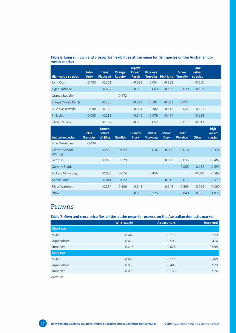
Table 6. Long run own and cross-price flexibilities at the mean for fish species on the Australian do-mestic market

High value speciesJohn Dory

Tiger Flathead

Orange Roughy

Bigeye Ocean Perch

Blue eye Trevalla Pink Ling

Silver Trevally

Low valued species

John Dory -0.493 -0.111 -0.033 -0.084 -0.132 -0.250

Tiger Flathead -0.462 -0.055 -0.069 -0.152 -0.039 -0.169

Orange Roughy -0.472

Bigeye Ocean Perch -0.236 -0.317 -0.101 -0.091 -0.054

Blue eye Trevalla -0.049 -0.188 -0.064 -0.302 -0.115 -0.037 -0.157

Pink Ling -0.053 -0.282 -0.042 -0.079 -0.427 -0.113

Silver Trevally -0.162 -0.053 -0.057 -0.617 -0.113

Low value speciesBlue

Grenadier

Eastern School

Whiting GemfishGummy

SharkJackass

MorwongMirror Dory

Silver Warehou Other

High Valued species

Blue Grenadier -0.424

Eastern School Whiting

-0.530 -0.022 -0.034 -0.056 -0.018 -0.374

Gemfish -0.086 -0.329 0.058 0.035 -0.487

Gummy Shark 0.066 -0.188 -0.599

Jackass Morwong -0.079 -0.074 -0.456 -0.040 -0.599

Mirror Dory -0.041 0.022 -0.315 -0.017 -0.579

Silver Warehou -0.254 0.106 0.045 -0.143 -0.505 -0.098 -0.360

Other -0.055 -0.125 -0.040 -0.536 -1.072

Prawns

Table 7. Own and cross-price flexibilities at the mean for prawns on the Australian domestic marketWild-caught Aquaculture Imported

Short run

Wild -0.447 -0.116 -0.379

Aquaculture -0.456 -0.595 -0.414

Imported -0.218 -0.028 -0.998

Long run

Wild -0.996 -0.114 -0.160

Aquaculture -0.030 -0.483 -0.929

Imported -0.096 -0.155 -0.976

Source: [4]


Oysters

Table 8. Own and cross-price flexibilities at the mean for oysters on the Australian domestic marketSydney Rock Oyster Pacific Oyster

Short run

Sydney Rock Oyster -0.804 0

Pacific Oyster -0.008 -0.262

Long run

Sydney Rock Oyster -1.359 0

Pacific Oyster -0.147 -0.353

Source: [5]


References1. Pascoe, S.; Schrobback, P.; Hoshino, E.; Curtotti, R. Demand Conditions and Dynamics in the SESSF: An

Empirical Investigation; FRDC: Canberra, 2021.

2. Wessells, C. R.; Miller, C. J.; Brooks, P. M., Toxic Algae Contamination and Demand for Shellfish: A Case Study of Demand for Mussels in Montreal. Marine Resource Economics 1995, 10, (2), 143-159.

3. Wakamatsu, H.; Miyata, T., Reputational damage and the Fukushima disaster: an analysis of seafood in Japan. Fisheries Science 2017, 83, (6), 1049-1057.

4. Schrobback, P.; Pascoe, S.; Zhang, R., Market Integration and Demand for Prawns in Australia. Marine Resource Economics 2019, 34, (4), 311-326.

5. Schrobback, P.; Pascoe, S.; Coglan, L., Impacts of introduced aquaculture species on markets for native marine aquaculture products: the case of edible oysters in Australia. Aquaculture Economics & Management 2014, 18, (3), 248-272.

6. Bath, A.; Mobsby, D.; Koduah, A. Australian fisheries economic indicators report 2017: financial and economic performance of the Southern and Eastern Scalefish and Shark Fishery; ABARES: Canberra, 2018.

7. Steven, A.; Mobsby, D.; Curtotti, R. Australian fisheries and aquaculture statistics 2018. Fisheries Research and Development Corporation project 2019-093; ABARES: Canberra, April. CC BY 4.0., 2020.

8. AFMA AFMA Catchwatch - Southern and Eastern Scalefish and Shark Fishery 2019; AFMA: Canberra, 2020.

9. Knuckey, I.; Boag, S.; Day, G.; Hobday, A.; Jennings, S.; Little, R.; Mobsby, D.; Ogier, E.; Nicol, S.; Stephenson, R. Understanding factors influencing under-caught TACs, declining catch rates and failure to recover for many quota species in the SESSF. FRDC Project No 2016-146; FRDC: Canberra, 2018.

© 2021 CSIRO and Fisheries Research and Development Corporation. All rights reserved.

Ownership of Intellectual property rights

Unless otherwise noted, copyright (and any other intellectual property rights, if any) in this publication is owned by the Fisheries Research and Development Corporation and CSIRO

This publication (and any information sourced from it) should be attributed to Pascoe, S., Schrobback, P. and Hoshino. E. 2021, How demand analysis can help improve fisheries and aquaculture performance. FRDC, Canberra, February 2021. CC BY 3.0

Creative Commons licence

All material in this publication is licensed under a Creative Commons Attribution 3.0 Australia Licence, save for content supplied by third parties, logos and the Commonwealth Coat of Arms.

Creative Commons Attribution 3.0 Australia Licence is a standard form licence agreement that allows you to copy, distribute, transmit and adapt this publication provided you attribute the work. A summary of the licence terms is available from creativecommons.org/licenses/by/3.0/au/. The full licence terms are available from creativecommons.org/licenses/by-sa/3.0/au/legalcode.

Inquiries regarding the licence and any use of this document should be sent to: [email protected]

Graphic design by Tracy Small, smalltdesign.com

Disclaimer

The authors do not warrant that the information in this document is free from errors or omissions. The authors do not accept any form of liability, be it contractual, tortious, or otherwise, for the contents of this document or for any consequences arising from its use or any reliance placed upon it. The information, opinions and advice contained in this document may not relate, or be relevant, to a readers particular circumstances. Opinions expressed by the authors are the individual opinions expressed by those persons and are not necessarily those of the publisher, research provider or the FRDC.

The Fisheries Research and Development Corporation plans, invests in and manages fisheries research and development throughout Australia. It is a statutory authority within the portfolio of the federal Minister for Agriculture, Fisheries and Forestry, jointly funded by the Australian Government and the fishing industry.

How demand analysis can help improve fisheries and aquaculture performance

FRDC Contact Details

Address: 25 Geils Court

Deakin ACT 2600

Phone: 02 6285 0400

Fax: 02 6285 0499

Email: [email protected]

Web: www.frdc.com.au

Researcher Contact Details

Name: Sean Pascoe

Address: CSIRO Oceans and Atmosphere Queensland Biosciences Precinct, 306 Carmody Road, St Lucia 4067 Australia

Email: [email protected]

In submitting this report, the researcher has agreed to FRDC publishing this material in its edited form.

Documents

How demand analysis can help improve fisheries and