econstorMake Your Publications Visible.

A Service of

zbwLeibniz-InformationszentrumWirtschaftLeibniz Information Centrefor Economics

Trebesch, Christoph; Zabel, Michael

Working Paper

The Output Costs of Hard and Soft Sovereign Default

CESifo Working Paper, No. 6143

Provided in Cooperation with:Ifo Institute – Leibniz Institute for Economic Research at the University of Munich

Suggested Citation: Trebesch, Christoph; Zabel, Michael (2016) : The Output Costs of Hard andSoft Sovereign Default, CESifo Working Paper, No. 6143, Center for Economic Studies and ifoInstitute (CESifo), Munich

This Version is available at:http://hdl.handle.net/10419/147397

Standard-Nutzungsbedingungen:

Die Dokumente auf EconStor dürfen zu eigenen wissenschaftlichenZwecken und zum Privatgebrauch gespeichert und kopiert werden.

Sie dürfen die Dokumente nicht für öffentliche oder kommerzielleZwecke vervielfältigen, öffentlich ausstellen, öffentlich zugänglichmachen, vertreiben oder anderweitig nutzen.

Sofern die Verfasser die Dokumente unter Open-Content-Lizenzen(insbesondere CC-Lizenzen) zur Verfügung gestellt haben sollten,gelten abweichend von diesen Nutzungsbedingungen die in der dortgenannten Lizenz gewährten Nutzungsrechte.

Terms of use:

Documents in EconStor may be saved and copied for yourpersonal and scholarly purposes.

You are not to copy documents for public or commercialpurposes, to exhibit the documents publicly, to make thempublicly available on the internet, or to distribute or otherwiseuse the documents in public.

If the documents have been made available under an OpenContent Licence (especially Creative Commons Licences), youmay exercise further usage rights as specified in the indicatedlicence.

www.econstor.eu

The Output Costs of Hard and Soft Sovereign Default

Christoph Trebesch Michael Zabel

CESIFO WORKING PAPER NO. 6143 CATEGORY 7: MONETARY POLICY AND INTERNATIONAL FINANCE

OCTOBER 2016

An electronic version of the paper may be downloaded • from the SSRN website: www.SSRN.com • from the RePEc website: www.RePEc.org

• from the CESifo website: Twww.CESifo-group.org/wp T

ISSN 2364-1428

CESifo Working Paper No. 6143

The Output Costs of Hard and Soft Sovereign Default

Abstract How costly are sovereign debt crises? In this paper we study output losses during sovereign default and debt renegotiation episodes since 1980. In contrast to previous work, we account for the severity of default and not only for its occurrence. Specifically, we distinguish between “hard” and “soft” defaults, using new data on debtor payment and negotiation behavior and on the size of haircuts towards private external creditors. We show that hard defaults are associated with a much steeper drop in GDP, of up to ten percent, compared to soft defaults, and address concerns of reverse causality and omitted variable bias. The results question the standard assumption that defaults trigger fixed and lump-sum costs. Instead, our findings are consistent with models assuming proportional output costs of default.

JEL-Codes: F340, F410, H630, G010.

Keywords: sovereign debt crises, debt restructuring, economic growth, reputation.

Christoph Trebesch* University of Munich

Department of Economics Schackstraße 4

Germany – 80539 Munich christoph.trebesch@econ.lmu.de

Michael Zabel University of Munich

Chair of Macroeconomics Ludwigstraße 28

Germany – 80539 Munich michael.zabel@econ.lmu.de

*corresponding author This version: 28.08.2016 We thank Henrik Enderlein, Gerhard Illing, Julian Schumacher, Uwe Sunde, Laura von Daniels, and participants in the Munich Macro Seminar for very helpful comments and suggestions. We build on the basic idea of the paper “The Cost of Aggressive Sovereign Debt Policies” (Trebesch, 2009), but use a different dependent variable and empirical approach. This paper supersedes that draft. All remaining errors are our own.

1 Introduction

How costly is a sovereign default? Answering this question is important for our theo-

retical understanding of sovereign debt1 and for policymakers in crisis situations. Past

empirical work on the cost of default commonly relied on a binary debt crisis measure

of default versus non-default. In this paper, we propose the use of more continuous

default measures to study output losses during debt crises. Specifically, we distinguish

between cases of “hard” and “soft” default based on a new procedural index that tracks

a government’s payment and negotiation behavior vis-a-vis foreign creditors during a

default spell. We also use a continuous outcome measure of debt crises, namely the

size of creditor losses or “haircuts” captured at the end of a debt crisis. Our results

show that the output loss during a debt crisis is much deeper for episodes of “hard”

defaults. This new stylized fact suggests that not only the incidence of default matters,

as implied by much of the previous literature, but also the scope and severity of default.

Our research design is motivated by the striking differences between debt crisis

events, as documented in case studies by Roubini and Setser (2004) or Sturzenegger and

Zettelmeyer (2007). On the one hand, there are cases such as Russia during the 1990s,

Ecuador 2008/2009 or Argentina 2002-2005, in which governments opted for a unilat-

eral payment moratorium, engaged in anti-creditor rhetoric, and at times even refused

to negotiate with their foreign banks and bondholders. These confrontational defaults

also involved high creditor losses (haircuts) of up to 70%. On the other hand, there are

debt crises that got resolved in a consensual manner, with close creditor consultations,

little (or no) missed payments, and low haircuts of around 10-20%. Examples include

Ukraine in 1999/2000 (and in 2015) or Uruguay in 2003.

The differences in crisis resolution strategies are influenced by a central trade-off for

distressed governments: on the one hand, governments can decide to adopt a confronta-

tional policy towards external creditors, by halting all debt payments, by demanding

high haircuts (debt relief), and by delaying negotiations and thereby postponing the

day until debt servicing is resumed. This strategy frees up resources that can be dis-

tributed to the domestic population during the default and may buy political support

at home. However, one can expect deep haircuts and confrontational debtor behavior

to also cause negative spillovers on the domestic economy and the financial sector (see

Panizza et al., 2009). One potential channel behind this is reputation: “hard” defaults

1Since Eaton and Gersovitz (1981), assumptions on the cost of default have crucially influenced thesetup and results of sovereign debt models (see the surveys by Eaton and Fernandez, 1995; Panizzaet al., 2009; Aguiar and Amador, 2014).

1

as in Argentina 2001 are likely to send a negative signal about fundamentals and worsen

country reputation more than “soft” defaults as in Uruguay 2003 (e.g. Cole and Kehoe,

1997). The expected outcome is a decline in access to external credit, less trade, less

investment and, thus, a drop in GDP (see Mendoza and Yue, 2012). The alternative

choice for governments in distress is to adopt a creditor-friendly stance, by continuing

debt payments to foreign banks and bondholders and by demanding low haircuts (little

debt relief). This strategy may mitigate the negative reputational effects of a default,

but will shift the burden to the domestic population, which can expect higher taxes

and less transfers during and after the default spell (D’Erasmo and Mendoza, 2016).

The main contribution of this paper is to take the heterogeneity in sovereign debt

crises seriously and to show in a stylized form that the output losses in a default

increase in the severity of default. This result casts doubt on one of the most widely

used assumptions in quantitative sovereign debt models, namely that defaults trigger

output costs that are fixed and lump-sum, irrespective of the type of default or the

size of haircuts. The notion that the output costs of default are proportional (rather

than lump-sum) shapes modeling in a fundamental way and also has “far-reaching

implications for policy analysis”, as emphasized by Corsetti and Dedola (2012).

We proceed in two steps. First, we analyze output during debt crises, since defaults

can take many years to resolve (sometimes more than a decade). In a second step, we

focus on post-crisis growth, i.e. output performance after countries exit default with

a debt restructuring. Our main explanatory variable during default is a measure on

“government coerciveness” towards creditors. This “coerciveness index” is based on a

new database on debt crisis resolution processes by Enderlein et al. (2012), which cat-

egorizes a government’s debtor policies on a scale from 1 (very creditor-friendly) to 10

(very confrontational). The dataset tracks government actions towards private external

creditors for each year throughout a debt crisis along nine dimensions of payment and

negotiation behavior. Debtor coerciveness shows a strong variation not only across debt

crises and defaulting countries, but also within crisis spells. This is advantageous com-

pared to a simple default dummy, since it allows us to exploit both the cross-sectional

and the time-series variation in debtor behavior. Our main explanatory variable after

debt crises is the size of haircuts, i.e. the scope of creditor losses implied by a debt

restructuring at the end of a default spell as measured by Cruces and Trebesch (2013).

In sum, we thus trace the output performance in “hard” and “soft” defaults over the

entire crisis episode, starting from the first missed payments to the conclusion of the

debt restructuring and the subsequent post-default period.

2

We find that coercive government behavior during default is associated with a sig-

nificantly worse output performance. In “hard” defaults, real GDP sees a strong and

long-lasting decline, while this is not the case in “soft” defaults in which the government

opted for a consensual stance towards creditors. This descriptive finding is confirmed

when we use annual per capita real growth as dependent variable and regress it on our

proxies for hard and soft defaults as well as economic fundamentals and fixed effects.

However, with cross-country panel data, it is difficult to identify the causal effect of

coercive debtor policies and high vs. low haircuts.2

In particular, we face two main identification challenges: (i) omitted variable bias,

as common shocks and/or socio-political changes could affect both output and coer-

civeness/haircuts, and (ii) reverse causality, since changes in output could explain the

type of default and not vice versa. To address the problem of omitted variable bias, we

include country and time fixed effects and a host of economic and political control vari-

ables, including the set of macro controls commonly used in the growth literature, but

also crisis duration, banking and currency crises, IMF programs, and political risk. We

also include a lagged dependent variable as a control and account for country-specific

time trends. Regarding reverse causality, we test whether past output performance

(growth) helps to predict debtor coerciveness later on, but find no evidence that past

economic growth drives current coercive behavior. Moreover, we attempt to disentan-

gle the role of expected and unexpected government coerciveness and tease out the

surprise component in debtor behavior by using forward-looking, start-of-year country

credit ratings. Taken together, the result of these checks are encouraging and help to

alleviate endogeneity concerns. Despite this, we cannot rule out that some unobserved,

time-varying confounder drives our results, so that the coefficients should be interpreted

with caution. We show strong conditional correlations and do not claim to show causal

effects.

With this caveat in mind, we show that the estimated coefficients for debtor coercive-

ness during default are both large and robust. In our most demanding specification,

moving from a soft default as in Uruguay 2003, to a coercive default as in Argentina

of 2005, is associated with a three percentage point lower growth rate in each default

year. Because debt crisis spells span more than 5 years, on average, this correlation

coefficient would translate to a more than 10 percentage point lower GDP level in hard

defaults as opposed to soft defaults (in the short- and medium-term).

2See Hebert and Schreger (2016) for a smart strategy to identify the output cost of default in onecrisis case, namely Argentina 2014.

3

While the differences are large during ongoing crisis spells (in each year of default), we

find no evidence for long-term effects post-crisis, i.e. once the country finally receives

debt relief and exits default. The coefficient of coercive debt policies is no longer

significant after the default exit and we also find no robust relationship between the size

of haircuts and post-crisis growth performance.3 This result may be due to the positive

impact of debt relief on post-crisis investment and growth, as suggested by Reinhart

and Trebesch (2016a). Another explanation is that countries settle with creditors and

exit default only after long delays and when growth prospects have already improved

(see Benjamin and Wright, 2009).

Our findings have implications for theory. Most importantly, they are not consistent

with the idea of lump-sum default costs. Most dynamic general equilibrium models

with defaultable debt assume fixed output costs of a default (for example Aguiar and

Gopinath, 2006; Yue, 2010; Arellano and Ramanarayanan, 2012; Hatchondo and Mar-

tinez, 2012; Chatterjee and Eyigungor, 2012; Hatchondo et al., 2014; Aguiar et al., 2013;

Cole et al., 2016, to name just a few). For calibration purposes, this literature often

uses an output loss of two percent in default years.4 Our results indicate that the costs

of default can be much higher or lower than that, depending on the severity of default.

We thus provide empirical backing for a small number of theory papers in which the

costs of default are proportional, that is, increase in the size of (expected) haircuts

(see e.g. Calvo, 1988; Bulow and Rogoff, 1989; Bolton and Jeanne, 2007; Corsetti and

Dedola, 2012; Adam and Grill, 2013; Arellano et al., 2013).5

Regarding the empirical literature, we are among the first to account for the mag-

nitude and the severity of sovereign defaults. Several earlier studies have emphasized

the important differences across debt crises events. Obstfeld and Taylor (2003), for

example, distinguish between “partial” and “full” defaulters, while Eichengreen (1991)

refers to “light” vs. “heavy” defaults. However, no contribution has yet quantitatively

analyzed how different crisis characteristics affect a country’s GDP growth in a large

sample of countries and crises. Most papers on the output costs of debt crises use a

binary default measure by Standard & Poor’s and conclude that defaults are associ-

ated with a steep drop in output, with estimates ranging from two to six percentage

points lower growth, depending on the sample and estimation method (see, in particu-

lar, Sturzenegger, 2004; Borensztein and Panizza, 2009; Furceri and Zdzienicka, 2012;

3See Kuvshinov and Zimmermann (2016) for an analysis on the short vs. long-term impact ofsovereign defaults on growth.

4This figure has been used with reference to Sturzenegger (2004).5For corporate debt, the assumption of proportional default costs is more established, see e.g. Zame

(1993) and Dubey et al. (2005).

4

Gornemann, 2016; Kuvshinov and Zimmermann, 2016). De Paoli et al. (2009) show

that the fall in output is particularly large when defaults are accompanied by banking

and/or currency crises. Tomz and Wright (2007) show that the relationship between

default and output since 1820 is unexpectedly weak. Levy-Yeyati and Panizza (2011)

use quarterly data to show that, on average, output contractions precede defaults and

that growth picks up after the quarter in which default occurs. More recently, Hebert

and Schreger (2016) tease out the cost of default in Argentina by focusing on exogenous

court rulings in New York and their effect on Argentinean stocks.

Despite this large literature, there is barely any work on the effects of different types

of debt crisis resolution (see also the empirical survey by Tomz and Wright, 2013).

In line with Cruces and Trebesch (2013), Asonuma and Trebesch (2016) and Catao

and Mano (2015), we conclude that it is crucial to account for the heterogeneity of

debt crises when studying their consequences.6 A dichotomous measure may be overly

simplistic and can introduce measurement error.

2 Theoretical considerations

The theory literature offers explanations why defaults are economically costly, and why

output costs could be larger in “hard” defaults with confrontational government behav-

ior and high haircuts. One group of papers emphasizes the role of reputational spillovers

and signaling. Grossman and van Huyck (1988) suggest that lenders differentiate be-

tween excusable defaults and cases of inexcusable debt repudiation. High creditor losses

and coercive debt policies that are not justified by a bad state of the economy could thus

lead to a deterioration of country reputation and, thereby, to “collateral damage” on

the domestic economy and lower output.7 Relatedly, Cole and Kehoe (1997, 1998) de-

velop a model of generalized reputation. Governments who are deemed untrustworthy

in one field will also be seen as untrustworthy in other fields. More recently, Sandleris

(2008) argues that the repayment behavior of sovereigns acts as a signal on country

fundamentals and government willingness (or ability) to undertake reforms and to pro-

6Asonuma and Trebesch (2016) study output losses in preemptive vs. post-default debt restructur-ings. Relatedly, a recent paper by Marchesi (2016) also uses the haircut data by Cruces and Trebesch(2013) and confirms our finding that more severe defaults (with high haircuts) are associated withlower growth. See also Trebesch (2009) for a similar setup using the coerciveness index. This papersupersedes that draft.

7Although we focus on proxies of coercive debtor behavior, this paper does not explicitly test forthe cost of “excusable” vs. “inexcusable” defaults.

5

tect property rights. Expropriative debt policies could thus affect agents’ beliefs both

at home and abroad, leading to less investments and lower growth.

These negative signaling and reputation effects can result in lower growth due to sev-

eral channels. Eaton and Gersovitz (1981) propose that a default results in exclusion

from international capital markets, which undermines a country’s ability to smooth

consumption and invest.8 Bulow and Rogoff (1989) emphasize the role of sanctions,

such as trade sanctions or legal sanctions, which increase in the share of debt that is

repudiated, resulting in a disruption of goods and asset trade and, thus, lower growth.

More recent contributions have emphasized spillovers on trade, investments, productiv-

ity and corporate access to foreign credit (Rose, 2005; Arteta and Hale, 2008; Trebesch,

2009; Mendoza and Yue, 2012; Sandleris and Wright, 2014), as well as the impact on

financial intermediation and the banking sector (Bolton and Jeanne, 2011; Gennaioli

et al., 2014b,a; Bocola, 2015).

The intuition behind our analysis is that the collateral damage of a sovereign default

is likely to be larger in hard default episodes, thus resulting in lower growth. Moreover,

there might be a direct financial sector channel: Gennaioli et al. (2014a) show that the

spillovers of a default on domestic and foreign banks are larger the higher the haircut

(using the same haircut data as in this paper).9

Taken together, these considerations help to rationalize our main empirical finding

that high expected haircuts and confrontational debt policies are associated with lower

growth during default.

Regarding the post-default period, there are at least two competing channels. On

the one hand, high haircuts and confrontational debtor policies could have lagged neg-

ative effects on growth, e.g. due to the spillover effects described above. On the other

hand, there is the channel of debt relief, which goes in the opposite direction. High

haircuts (and confrontational policies leading to high haircuts) reduce government in-

debtedness more significantly. This debt relief effect can allow countries to exit a debt

overhang situation and reduces the risk of future default, possibly improving growth

prospects (see Arslanalp and Henry, 2005; Reinhart et al., 2012; Reinhart and Trebesch,

2016a). While we account for debt relief by controlling for the debt to GDP ratio after

8In Kletzer and Wright (2000) and Wright (2002) exclusion and punishment does not occur inequilibrium. However, recent models in which defaults do occur in equilibrium continue to assumecredit market exclusion, at least temporary exclusion (e.g. Arellano, 2008; Yue, 2010).

9As in most of the existing literature, we do not analyze the underlying channels at work here,meaning that we do not test whether the observed link between default and growth can be explainedby sanctions, reputational damage and/or signaling. Indeed, it is very challenging to identify thereputation or signaling channels empirically.

6

the restructuring, the link between haircuts and post-default growth is theoretically

ambiguous and, thus, an empirical question.

3 Empirical approach and data

Existing work on the link between default and growth, such as Sturzenegger (2004) and

Borensztein and Panizza (2009), typically regresses annual per capita real growth on

a dummy for the start of default, lagged values of this dummy, and a set of standard

control variables as used in the cross-country growth literature. This binary categori-

sation of sovereign defaults hides the substantial variation in crisis characteristics. In

the following, we therefore propose using more continuous measures of default severity.

3.1 Classifying hard and soft sovereign defaults

We distinguish between “hard” and “soft” defaults by building on two distinct empiri-

cal measures on the heterogeneity of debt crisis events. The first measure is the index

of debtor coerciveness constructed by Enderlein et al. (2012), which is procedural and

captures differences in crisis characteristics during default, in particular the payment

and negotiation behavior of governments towards foreign creditors. The second mea-

sure is the main outcome of debt renegotiations, namely the size of creditor losses or

“haircuts” implied in debt restructuring agreements that resolve a default. Based on

these two measures, we seek to trace the relationship between debtor default behavior

and GDP over the entire debt crisis episode — from the start of default, over the whole

default and debt renegotiation period (which lasts an average of 6.3 years in our sample)

and up to five years after the crisis ends with a final restructuring.

The coerciveness and haircut measures both have their strengths and weaknesses for

the purpose of this analysis. The main advantage of using haircuts is that it is an intu-

itive measure that can be computed based on observable terms of a debt restructuring

agreement. The disadvantage, however, is that haircuts are a snapshot measure that

can only be observed once – at the end of a debt renegotiation period, which can take

many years. An illustrative example is the default of Peru, whose debt crisis lasted

from the mid-1980s until the late 1990s, when the default was finally cured with the

Brady deal of 1997. During these 15 years, Peru’s debt policy vis-a-vis its foreign cred-

itors varied substantially. The government’s stance was very confrontational after the

inauguration of President Garcia in 1985, who immediately imposed a unilateral debt

7

Figure 1: Stylized crisis timeline and research design

Start of default / renegotiations Final deal

t

Pre-crisis period

Explanatory variables:•Realized haircut, lagged•Coerciveness, lagged

Explanatory variables:•Government coerciveness

index (year by year) •Expected haircut

Post-restructuring period(after default exit)

Debt renegotiation / in default(crisis period, avg.: 6.3 years)

moratorium. After President Fujimori took over in 1990, Peru’s debt policies became

much more cooperative and negotiations were resumed. This variation in debtor policy

is captured accurately by the coerciveness index10, while a haircut is only available for

the end of default in 1997. In principle, one can make the argument that creditors

quickly form expectations on the scope of losses which they are likely to suffer and that

the expected haircut will be roughly in line with the realized final haircut. However,

for longer crises, such as the one in Peru, it is far-fetched to use the 1997 haircut as

a proxy for loss expectations in the mid- or late 1980s. The advantage of the index of

debtor coerciveness is that it is time varying and observable for each year throughout

the debt crisis. It therefore allows us to capture both the within-crisis variation and the

cross-sectional variation in debtor policies. However, as any newly constructed index,

the coerciveness index can be criticized as being too broad or too narrow, or for not

using the right criteria or weighting scheme (see the detailed discussion in Enderlein

et al., 2012).

Against this backdrop, we use both the procedural coerciveness index and the out-

come variable haircuts to classify hard and soft defaults. Specifically, we focus on the

coerciveness index as our main explanatory variable during a default spell, and use

haircuts as our preferred measure for the post-default period. Our research design is

illustrated in Figure 1, which shows a stylized debt crisis timeline.

10More specifically, the coerciveness index in Peru increases from 2 at the start of default in 1982to 8 in the year 1985, when Garcia became president. Throughout Garcia’s presidency, the indexfluctuates at a value above 5 and then declines gradually after Fujimori takes office (from 5 in 1990 to1 in the settlement year 1997).

8

3.2 The coerciveness index

The index of debtor coerciveness (or coerciveness index) was coded from quantitative as

well as qualitative sources, including 20,000 pages of articles from the financial press.

The idea of categorising different types of debtor behavior towards creditors is not

new. Authors like Aggarwal (1996), Andritzky (2006), Cline (2004) or Roubini (2004)

all suggested that debt policies and restructuring processes vary on a spectrum from

“soft” to “hard” or from “voluntary” to more “involuntary”. However, Enderlein et al.

(2012) provide the first comprehensive and systematic dataset suitable for econometric

analysis.

The construction of the index mirrors the views of financial market participants,

policymakers, and researchers on how fair debt restructuring processes should look like.

An essential point of reference were the “good faith” criteria outlined in the IMF’s

lending into arrears policy International Monetary Fund (1999, 2002), as well as the

list of best practices in the IIF’s “Principles for Stable Capital Flows and Fair Debt

Restructuring in Emerging Markets” (Institute of International Finance, 2013). These

two “how to” manuals of fair debt restructuring play a central role in debt crises and

are well known by officials and investors alike. They therefore shaped the way the

sub-indicators of the coerciveness index were defined and coded. Also previous research

on “coercive” defaults guided the index design, in particular the criteria proposed by

Cline (2004) and Roubini (2004).

The final index captures coercive measures which governments adopt towards their

private external creditors, such as foreign banks or bondholders. It consists of nine sub-

indicators, each of which gauges observable government actions vis-a-vis creditors. Each

sub-indicator is a dummy variable, which is coded as one if the respective action by the

government can be observed in a given year, and zero otherwise. The sub-indicators can

be grouped into two broad categories: (1) “Indicators of Payment Behavior”, capturing

government actions that have an immediate effect on the financial transfers to interna-

tional banks or bondholders, and (2) “Indicators of Negotiation Behavior”, measuring

negotiation patterns and confrontational rhetoric of governments. By definition, the

index is coded for debt crisis episodes only, where the start of a debt crisis is defined

as either missed payments (legal default) or the announcement of a debt restructuring

by a key government official (see section 3.4. below for more details).

Enderlein et al. (2012) give the exact definitions of and the theoretical rationale for

each sub-indicator and provide the detailed coding procedures, descriptive statistics

and stylized facts on the index. Here, we summarize each sub-indicator briefly.

9

The indicators of government payment behavior during debt crises are the following:

1. Payments missed? (yes/no): The first sub-indicator is coded 1 whenever a

government misses interest or principal payments on its bonds or commercial

loans beyond the grace period. Accordingly, it takes the value of 0 whenever

the sovereign manages to restructure its debt pre-emptively, before running into

arrears. Most debt crises do involve missed payments, but there are many excep-

tions too. Examples of restructurings without missed payments include Algeria

and Uruguay in the 1980s, or Uruguay in 2003.

2. Unilateral payment suspension? (yes/no) The second sub-indicator captures

whether the sovereign did unilaterally suspend payments to its creditors, i.e. with-

out a previous agreement with and/or consultations with creditors. This indicator

enables us to differentiate between outright defaults on the one hand and “ne-

gotiated defaults” on the other (Bulow and Rogoff, 1989). Even in severe crises,

officials can reach out to creditors and seek preventive debt roll-overs or other

forms of bridge financing. Despite this, two thirds of payment suspensions occur

unilaterally and without prior agreement or consent.

3. Full moratorium, incl. interest payments? (yes/no): The third indicator

captures full moratoria, meaning the suspension of all sovereign debt payments to

private creditors, including interest. Partial debt servicing is a recurring demand

of banks and bondholders during debt crises and also the (Institute of Interna-

tional Finance, 2013) demands continuing interest payments as a sign of good

faith. A complete suspension of payments can therefore be interpreted as par-

ticularly coercive debtor policy and signals a government’s unwillingness to pay.

Full moratoria only occur in around a quarter of all annual crisis observations.

4. Freeze on foreign assets? (yes/no): The fourth indicator is coded 1 when the

government issues emergency decrees that effectively lead to a freeze of creditor

assets in the country. Past crises have sometimes been accompanied by capital

and exchange controls that prohibit domestic firms to service their debt to foreign

banks or bondholders. This type of asset freezes are a particularly tough debtor

policy and are observed only on rare occasions, e.g. in Argentina in 1982 and

2002, or in Ukraine and Pakistan in 1998.

10

The indicators of government negotiation behavior during debt crises are:

5. Breakdown or refusal of negotiations? (yes/no): This indicator measures

whether governments refuse to engage in negotiations with its creditors and/or

whether government actions result in a breakdown of debt negotiations for a pe-

riod of three months or more in a given year. Regular and continuous dialogue

between the sovereign and its creditors are an essential prerequisite for the con-

sensual solution of a debt crisis. Nonetheless, government-induced delays and

refusals to negotiate are quite common and take place in almost half of all crisis

years.

6. Explicit moratorium or default declaration? (yes/no): Does a key gov-

ernment actor (president, prime minister, minister of finance or economy, or the

president of the central bank) officially proclaim the decision to default? Explicit

default declarations are rare since most governments miss payments as quietly

and discretely as possible. However, in cases such as Peru 1985, Ecuador 1999

and Argentina 2001, the decision to default was publicly announced and accom-

panied by anti-creditor rhetoric, thus resembling a “declaration of war” against

foreign banks and bondholders.

7. Explicit threats to repudiate on debt? (yes/no): Does a key government

actor publicly threaten to repudiate sovereign debt owed to foreign private cred-

itors? Open threats to cancel debt payments or to impose an indefinite morato-

rium are rare, but they can be an effective strategy to extract more concessionary

terms from creditors. Examples include repudiation threats of Chilean President

Pinochet in 1986, or President Correa of Ecuador in 2008 who threatened to de-

clare large parts of the government’s foreign debt as “odious” and “illegitimate”.

8. Data disclosure problems? (yes/no): This indicator captures data disclosure

problems, i.e. cases in which the government refused to provide crucial debt-

related information and cases in which there is an open dispute due to inaccurate

government data. The provision of reliable data on debt stocks or foreign exchange

reserves constitutes a basic requirement for creditors to evaluate a country’s ca-

pacity to repay and to assess the terms of a debt exchange proposal. Data-related

disputes are therefore coded as a coercive action. Examples include Brazil 1987,

Peru 1996 or Ecuador 2008/09 where data issues have been a central stumbling

block for crisis resolution.

11

Figure 2: Construction of the coerciveness index

Note: This figure illustrates the construction of the coerciveness index. It is taken from Enderlein

et al. (2012).

9. Forced and non-negotiated restructuring? (yes/no): The final indicator is

coded 1 whenever the restructuring was not negotiated with creditors but unilat-

erally imposed by the government. The idea is to identify debt exchanges that

are implemented without prior creditor consultations. Forced and non-negotiated

restructurings are rare and constitute a strong sign of coercive debt policies. The

restructuring of Argentina in 2005 as well as a forced debt roll-over in Peru of

1986 are among the few examples.

The final coerciveness index is additive, defined as equally weighted sum of the 9

binary sub-indicators.11 An index value of 0 applies in normal times without default

or debt renegotiations, i.e. if the government pays back its debt in full and on time.

A value of 1 is assigned if a government announces a debt restructuring (crisis start),

but does not fulfill any of the 9 coerciveness criteria in that year. This means that

there are cases for which the index takes the value of 1 even if the country misses

no payments (no legal default). For example, debt crisis spells like Uruguay 2003 or

Algeria 1992 are categorized as 1, since both countries restructured their debt with a

haircut, but without missing payments, without threats, and in close coordination with

creditor groups. During debt crisis spells, the index thus ranges from a minimum of 1,

indicating a debt renegotiation period with very cooperative government behavior, to

10, for particularly aggressive debt policies and a full moratorium. Figure 2 illustrates

11The results are very similar when weighting the sub-indicators using principal component analysis.

12

the construction of the coerciveness index graphically. Moreover, Figure A.1 in the

Online Appendix shows the distribution of the coerciveness index and reports summary

statistics for each sub-indicator.

3.3 The size of haircuts

We now move on to our second main explanatory variable: the size of haircuts nego-

tiated between the government and its external creditors. This is the central outcome

of the debt restructuring process. Since haircuts are a straightforward measure there is

less need for detailed explanations as was the case for the coerciveness index above.

Specifically, we use the database of investor losses by Cruces and Trebesch (2013) that

measures creditor haircuts in restructurings between 1970-2010 based on the method-

ology proposed by Sturzenegger and Zettelmeyer (2008) as:

HSZ = 1− Present V alue of New Debt (r)

Present V alue of Old Debt (r),

where r is the discount factor employed to calculate the present value of old and new

debt instruments.

Building on Cruces and Trebesch (2013) we focus on haircuts in “final” debt restruc-

turings only. Final deals are those that enable countries to cure the default and exit

a crisis spell without a renewed default in the following 4 years. This focus on final

restructurings is in the spirit of related work such as Cline (1995), Arslanalp and Henry

(2005) and Reinhart and Trebesch (2016a) who also study the outcome of final deals

and pay less attention to intermediate restructurings like most debt operations of the

1980s that only implied short-term relief. Peru can again serve as an example, since

its restructuring of 1983 is not coded as final, because it was merely a two-year debt

rollover and did not cure the default. Indeed, Peru continued to miss payments and did

so until 1997.

The number of final restructurings in our sample are 30 cases, including the Brady

debt exchanges of the 1990s as well as all main recent emerging market bond exchanges

such as Russia 2000 or Argentina 2005. Importantly, this haircut sample closely matches

the sample for which we also have the prodedural coerciveness data (during default),

so that we can directly compare results for both measures. Figure A.2 shows how the

haircuts in our sample are distributed over time and reports basic summary statistics.

13

Finally, Figure 3 shows a scatter plot of haircuts (in final deals) and the coerciveness

index by debt crisis events (computed as average yearly index value for each crisis

spell). As can be seen, the relationship between these two measures is very tight, with

a correlation coefficient of close to 0.70. This suggests that coercive actions during

default are a good predictor for the degree of realized creditor losses, i.e. for the size of

haircuts that is negotiated at the end of a default spell.

Figure 3: Haircuts and coerciveness index - scatter plot

020

4060

80

Hai

rcut

in %

0 1 2 3 4 5 6 7 8 9

Average coerciveness over crisis period

Correlation coefficient: 0.6966

Note: This graph shows a scatter plot between the size of haircuts (in final restruturings of each crisis

spell) and the coerciveness index (as yearly averages over each crisis spell).

3.4 Default coding and sample composition

Our analysis spans the years between 1980 and 2009 and includes 61 developing and

emerging market economies. We selected this sample as follows. Given our focus on

debt crises involving commercial creditors, we first excluded those countries which had

only very limited access to foreign private credit over our sample period. Specifically,

we drop all countries that have been classified by the IMF and the World Bank as

highly indebted poor countries (HIPCs) and typically owe more than 80% of their

external debt to official (not private) creditors. We also drop small countries with a

population of less than 1 million (as measured at the end of our sample period) and

exclude all advanced economies in order to make our sample as homogeneous as possible.

Moreover, we drop a few defaulters for which no sufficient qualitative information on

the debt renegotiation process and on debt payments was available (Cote d’Ivoire,

14

Cuba, Gabon, Iran, Jamaica, Kenya, Paraguay, Trinidad and Tobago and Vietnam)

and countries whose debt restructurings took place in the context of wars and state

dissolution, namely Iraq and the successor states of the Socialist Republic of Yugoslavia.

The resulting set of 61 countries includes 25 defaulting countries, which experienced at

least one debt crisis during our sample period, as well as a 36 non-defaulters. Table

A.1 in the Online Appendix shows all countries and years, including a list of debt crisis

episodes studied here.

To measure sovereign defaults, we follow the widely used default definition of Stan-

dard & Poor’s and rely on their annual default list. S&P codes a government as being

in default if the government misses payments on either interest or principal of bonds or

bank loans on the due date or, alternatively, if it announces a debt exchange offer that

leads to less favorable conditions for creditors than those in the original contracts (see

Appendix 1 of Standard & Poor’s, 2011). All in all, our sample covers 1,638 annual

country observations, of which 210 observations are default years.

4 Output performance during default

4.1 Preliminary analysis and stylized facts

We start our analysis of growth during debt crises with a graphical view at the data.

Figure 4 illustrates the performance of real GDP per capita from three years before

until five years after start of default. The starting year of a crisis is labeled as year zero

(black vertical line) and GDP is normalized to 100 in the year prior to the start of the

debt crisis, as defined above.

Panel A depicts the average GDP performance for the 31 debt crises in our sample.12

In line with Levy-Yeyati and Panizza (2011), we find that the onset of a debt crisis

roughly marks the beginning of recovery. On average, GDP starts to decline prior to

a debt crisis and shrinks by another four percent in the year of default. Immediately

after, however, output starts to recover and reaches its pre-crisis level four years later.

In Panel B of Figure 4, we divide the sample into cases of hard and soft defaults.

For this purpose, we compute the average value of the coerciveness index over each

12This number is larger than the number of defaulting countries (25) due to the fact that somecountries defaulted multiple times (see Table A.1 in the Online Appendix). Note also that we dropfollow-up defaults that are very close in timing and thus effectively in the same crisis spell, i.e. thosethat occur in the time window [-3,+5]. Specifically, we exclude Romania 1985, Morocco 1986, Uruguay1987 and 1990, South Africa 1989, and Venezuela 1990.

15

Figure 4: Real GDP around the start of default

(a) Panel A: All defaults

8085

9095

100

105

110

115

120

Rea

l GD

P p

er c

apita

(T

−1=

100)

−3 −2 −1 0 1 2 3 4 5

Years around start of default

(b) Panel B: Hard and soft defaults

8085

9095

100

105

110

115

120

Rea

l GD

P p

er c

apita

(T

−1=

100)

−3 −2 −1 0 1 2 3 4 5

Years around start of default

Note: The solid lines show average real GDP per capita from three years before until five years after

the start of default. The dashed lines are 90% confidence intervals. Real GDP per capita is normalized

to 100 in the year before the start of default. Panel A includes the full sample of default episodes,

while Panel B splits the sample at the median average coerciveness across crisis episodes, which is

3.4. Cases of soft default are shown in red (coerciveness values larger than 3.4) while soft defaults are

shown in blue (average coerciveness smaller than 3.4).

debt crisis and cut the sample at the median value, which is 3.4. The result are 15

cases categorized as soft defaults (with an average government coerciveness index of

less than 3.4) and 16 cases of hard default (with average coerciveness larger than 3.4).

16

As can be seen, output behaves very differently for both groups. In soft default spells,

output drops only marginally in the first crisis year and quickly picks up afterwards.

However, the picture drastically differs for hard defaults, with an output collapse of

around seven percent in the first crisis year and a further decline during the subsequent

year. Thereafter, the economy recovers only sluggishly. Five years after the outbreak

of the crisis, real GDP remains more than five percentage points below its pre-crisis

level. The result of quick recoveries by Levy-Yeyati and Panizza (2011) can thus not

be confirmed for hard defaults, since these cases do not see a rebound after the first

default year. The difference in real GDP performance between hard and soft defaulters

is statistically significant at the 10% level.

4.2 Regression analysis

In this subsection, we analyze the relationship between debtor coerciveness and GDP

in a more systematic way. Our main empirical model looks as follows:

Growthi,t = αi + αt + βDefaulti,t + γCoerci,t + δXi,t + εi,t , (1)

where Growthi,t is the annual real per capita GDP growth rate, Coerci,t is the time

varying coerciveness index measured in each debt crisis year, Defaulti,t is a binary

variable capturing sovereign defaults according to S&P (defined as 1 in years with

missed payments or debt restructuring and 0 otherwise), Xi,t is a vector for our set

of macroeconomic controls, and αi and αt stand for country and time fixed effects,

respectively.

Formally, equation 1 is a multiplicative interaction model in which we interact the

default dummy with the coerciveness index, which is only coded during default spells. γ

should thus be interpreted as the coefficient of an interaction term, since the coerciveness

index is always 0 in non-crisis years and its value in crisis years is equal to multiplying

the default dummy with the index of coerciveness. The sum β + γCoerci,t will thus

pick up the joint effect of a default and coerciveness on growth. Intuitively, this allows

us to assess the correlation of default and growth, conditional on the scope of debtor

coerciveness during the default.

To assure that the model is properly identified, the constitutive term Defaulti,t has

to be included in all specifications and its coefficient can no longer be interpreted at face

value whenever the interacted variable Coerci,t is also included. In this econometric

setting, the Defaulti,t coefficient no longer shows an unconditional marginal effect as

in a standard multivariate regression (see Brambor et al., 2006). The high correlation

17

between Defaulti,t and Coerci,t is likely to increase the estimated standard errors

(see Goldberger, 1991, chapter 23). This is a relevant concern, but it also stacks the

odds against us, since we are more likely to find insignificant coefficients for Coerci,t.

Moreover, Kennedy (2003) and (Goldberger, 1991) explain that multicollinearity can

actually be desirable if one is interested in the joint effect of two highly correlated

variables, which is the case here. Indeed, multicollinearity in our context will tend to

lower the variance of the estimated effect of interest, β + γCoerci,t.

Before estimating our main model, we start with a bare bones specification in Column

1, in which we regress the annual real GDP growth per capita (Growthi,t) on a dummy

variable capturing whether a country is in default (Defaulti,t) and on a set of year

dummies to control for global (i.e. not country-specific) time trends using pooled OLS.

In line with previous research, the default dummy turns out highly significant and

negative (Table 1, Column 1). The coefficient value of around -1.1 indicates that being

in a debt crisis reduces a country’s GDP growth by around 1.1% per year.

In model 2, we include both the binary default dummy and Coerci,t. As can be seen,

the coerciveness index turns out highly significant with a large negative coefficient. A

one notch increase in the index is associated with 0.6 percentage point lower real GDP

growth for each crisis year. We next add a set of macro controls (Xi,t) that is commonly

used in the cost of default literature (Sturzenegger, 2004; Borensztein and Panizza, 2009;

Levy-Yeyati and Panizza, 2011). Specifically, we include investment to GDP (InvGDP),

rate of population growth (∆Pop), log of total population (Log(Pop)), percentage of

the population that completed secondary education (SecEdu), lagged annual growth

of government consumption (GovtConst−1), the Freedom House index of civil liberties

(CivLib), annual change in terms-of-trade (∆ToT ), openness, as proxied by the ratio

of imports plus exports to GDP (Openness), and a dummy variable for banking crises

(BankingCrisis). Table A.2 in the Online Appendix provides a detailed description of

each control variable and its source.

Column 3 shows that the coefficient and significance of the default dummy barely

changes when adding the set of growth controls. Moreover, the results and the estimated

default coefficient are almost identical to previous studies on the cost of default such as

Panizza et al. (2009) and Sturzenegger (2004).13 Column 4 shows that the coerciveness

13Panizza et al. (2009) estimate a default dummy coefficient of -1.3, compared to -1.1 in Column 3.We also get a result very similar to Sturzenegger (2004), once we replace the default dummy (for eachyear during default) with a dummy variable that only captures the first and the second year of a debtcrisis. Debt crises can then be associated with a decline in GDP growth of around 2% during the firsttwo years of default.

18

Table 1: GDP growth and government coerciveness during default

(1) (2) (3) (4) (5) (6) (7) (8)Plain Plain With With Average Coerc vs. Main With

controls controls Coerc AvgCoerc model Haircuts

Default -1.140** 1.134 -1.099** 0.370 0.428 1.827 1.129 0.325(Dummy) (0.468) (0.713) (0.442) (0.751) (0.959) (1.328) (1.006) (0.829)Coerc -0.627*** -0.422** -0.414* -0.566**(Index) (0.192) (0.202) (0.246) (0.221)Average -0.433* -0.358Coerc (0.262) (0.345)Haircuts -0.035*(expected) (0.020)Inv/GDP 17.683*** 17.588*** 17.699*** 17.792*** 17.637*** 18.044***

(2.077) (2.057) (2.074) (3.492) (3.497) (2.078)∆Pop -0.339** -0.319** -0.315** -0.074 -0.087 -0.328**

(0.144) (0.142) (0.143) (0.344) (0.345) (0.144)Log(Pop) -0.093 -0.084 -0.087 -3.398 -3.491 -0.111

(0.090) (0.089) (0.090) (3.776) (3.783) (0.091)SecEdu 0.008 0.009 0.009 -0.004 -0.004 0.009

(0.010) (0.010) (0.010) (0.035) (0.035) (0.010)GovtConst−1 0.112*** 0.112*** 0.112*** 0.089*** 0.088*** 0.110***

(0.020) (0.020) (0.020) (0.018) (0.018) (0.020)CivLib -0.092 -0.104 -0.112 -0.053 -0.021 -0.108

(0.091) (0.090) (0.091) (0.217) (0.218) (0.091)∆ToT 10.364*** 10.240*** 10.375*** 9.903*** 9.838*** 10.475***

(1.220) (1.203) (1.209) (1.356) (1.351) (1.207)Openness -0.003 -0.002 -0.003 -0.007 -0.007 -0.003

(0.002) (0.002) (0.002) (0.014) (0.014) (0.002)BankingCrisis -2.533*** -2.422*** -2.470*** -2.175** -2.185** -2.471***(Dummy) (0.820) (0.815) (0.810) (0.842) (0.850) (0.820)

Observations 1,638 1,638 1,113 1,113 1,113 1,113 1,113 1,113Countries 61 61 45 45 45 45 45 45Time FE YES YES YES YES YES YES YES YESCountry FE NO NO NO NO NO YES YES NOR2 0.129 0.135 0.354 0.359 0.357 0.322 0.321 0.357

Note: The dependent variable is the annual growth rate of real GDP per capita, measured in percentage

points. The key explanatory variable is the coerciveness index, Coerc, but we also use the average

coerciveness index over a debt crisis, as well as the (expected) haircut size, using the same haircut value

for each crisis year until the final restructuring. All specifications include a (non-reported) constant.

Robust standard errors are given in parentheses. ***, **, and * denote significance at the 1, 5, and 10

per cent levels, respectively.

index remains significant when including this same set of macro controls, although the

coefficient size drops slightly, from -0.63 in the bare-bones model to -0.42.

In a next step, we distinguish between average coerciveness across crises and time-

varying coerciveness within the same crisis. Our motivation of doing so is that the

pooled OLS results mask where the explanatory power of Coerci,t stems from. Given

the annual coding, the significant coefficient could result (i) from variation in the coer-

civeness index across different default episodes, or (ii) from variation in the coerciveness

index within default episodes, or (iii) from both.

19

The results in Column 5 of Table 1 indicate that the differences in the level of debtor

coerciveness across crises play an important role. Average Coerc is defined as the mean

of the annual coerciveness observations observed in each debt crisis episode, so that

this measure varies across but not within debt crises. The resulting coefficient of -0.43

and is significant at the 10% level. This finding underlines our previous descriptive

insight that debt crises with more coercive average payment and negotiation patterns

are associated with substantially weaker GDP growth (Figure 4).

Furthermore, in Column 6 we aim to distill the role of within-crisis variation in

the coerciveness index. For this purpose, we estimate a panel model with country

fixed effects and then run a horse race between Average Coerc and the time varying

coerciveness index Coerc. While the fixed effects absorb the cross-country variation in

debtor coerciveness, adding Average Coerc accounts for the fact that some countries

in our sample defaulted multiple times. This implies that the coefficient of Coerc will

now solely pick up the variation in debtor coerciveness within the same debt crisis. As

can be seen, Coerc is significant at the 10% level with a quantitatively large coefficient,

which supports the view that also the within-crisis variation matters for our main result.

Overall, we thus conclude that the coerciveness index helps to explain output growth

both within and across debt crisis events.

We move on to estimate our main model of equation (1). The results are shown in

Column 7. The only difference to Column 4 is that we now include country fixed effects,

which pick up time-invariant country-specific characteristics. This is important since it

allows us to account for differences in the strength of institutions or any other source

of unobserved heterogeneity that could drive both the level of government coerciveness

and output performance during crises. Because we drop AvgCoerc, the coerciveness

index now captures both the time variation within debt crises as well as the variation

between crises in the same country. The resulting coefficient of -0.57 implies that a

one-notch increase in the coerciveness index is associated with a 0.57 percentage point

lower growth in that country. Put differently, moving from a coerciveness index level of 1

(Dominican Republic in 2005) to a level of 7 (Dominican Republic in 1990) is associated

with a 3 percentage point lower growth rate in each default year, after controlling for

standard macroeconomic controls, global trends, and the default effect per se. Given

that the average debt crisis takes more than five years to resolve, the cumulative growth

differences are very large.

Maybe the best way to illustrate our main finding is the interaction graph of Figure 5,

which shows real GDP growth in default spells, conditional on the level of government

20

Figure 5: Real GDP growth during default conditional on debtor coerciveness

−6

−4

−2

02

4A

nnua

l GD

P g

row

th c

ondi

tiona

l on

debt

or c

oerc

iven

ess

0 1 2 3 4 5 6 7 8 9Coerciveness index value

Note: This figure shows the estimated output loss during default for different levels in the debtor

coerciveness index. The vertical axis plots the joint estimate β + γCoerci,t based on our baseline

specification (7) of Table 1. The dotted lines are 90 percent confidence bands. The main message of

this graph is that defaults are only associated with lower growth if the coerciveness index values is 4

or higher (where the upper confidence band exceeds the zero horizontal line). Soft defaults with few

coercive actions towards creditors see no significant growth decline.

coerciveness (using the fully specified model of Column 7). The vertical axis shows

β + γCoerci,t, i.e. the expected growth impact of a default for different levels in the

debtor coerciveness index, while the dotted lines show 90 percent confidence bands. The

bottom line of the figure is that defaults are only associated with significantly lower

growth if governments adopt at least a medium level of coerciveness towards their for-

eign creditors. This is because the upper confidence band is above the 0 horizontal line

only for index values above 4. This is slightly higher than the sample mean coerciveness

of 3.6. At an index value of 7, the estimated joint effect of a coercive default is large,

indicating three percentage points lower growth each year. In contrast, soft defaults

with index values of 1 or 2 do not see a significant decline in growth compared to normal

times.

In a complementary step, we now replace the coerciveness index in equation (1)

with the size of haircuts measured at the end of a default spell. Specifically, we take

the estimated haircut and use its value for each crisis year in the run up to the final

restructuring. The resulting variable can be interpreted as the expected size of haircuts,

but should be taken with care given that the debt crises often span more than 10 years.

It is unrealistic that markets correctly anticipate the haircut imposed 10 or 15 years

21

later. Moreover, haircuts tend to be higher in protracted defaults, as documented

by Benjamin and Wright (2009).14 The haircut measure used in this specification is

therefore closest to the AvgCoerc measure of Column 5. Indeed, the pairwise correlation

between those two is 70%, as shown in Figure 3.

Column 8 shows that the haircut variable has a negative coefficient of -0.035 and is

significant at the 10% level. This suggests that increasing the haircut by 10 percentage

points is associated with a reduction in annual GDP growth of 0.35% during defaults.

Put differently, a shift from a haircut of 10% (as in Uruguay 2003) to a haircut of 77%

(as in Argentina 2005) is associated with 2.5% lower growth.

4.3 Robustness checks

This section addresses additional identification challenges and tests the robustness of

our main model of eq. (1).

Autocorrelated standard errors: It is possible that the regression residuals are

serially correlated, in particular since past growth rates are known to be a good predic-

tor of contemporaneous and future growth. Autocorrelation in the error terms would

bias the estimated standard errors downwards and thus overestimate the t-statistics

(Cameron and Tivedi, 2005). One way to address this problem, is to add a lagged value

of our dependent variable (Growthi,t−1), which we do in Column 1 of Table 2. As can

be seen, the results remain largely unaltered and the coerciveness index continues to

be strongly significant and negative.

While including lagged GDP growth as an explanatory variable solves the problem of

autocorrelated error terms in our model, this step can also introduce bias, as famously

pointed out by Hurwicz (1950) and Nickell (1981). The fixed effects center all variables

by country which induces a correlation between the centered lagged dependent variable

on the one hand and the centred error term on the other. This “Nickell bias” is of

order 1/T , such that it decreases with rising T but is very serious for panels with a

short time horizon. A sample of T=30, as it is the case here, may still result in a bias

of up to 20% of the true coefficient value, as shown by (Judson and Owen, 1999). In

order to correct for the “Nickell bias”, we follow Beck and Katz (2011) and Judson

and Owen (1999) and move back to a simple OLS framework (without country fixed

effects). Column 2 shows that our results continue to hold, although the coerciveness

index decreases in size and remains significant only at the 10% level. Another approach

14The link between default duration and debtor coerciveness is discussed in the robustness section.

22

to tackle the Nickell bias is to run a GMM estimation.15 Column 3 shows the result:

the coerciveness index remains significant, with a coefficient that is similar to our main

specification. We therefore conclude that our baseline estimation results are robust

even after accounting for the possibility of serially correlated errors.

Controlling for crisis duration: One important fact about debt crises is that they

vary greatly in length. For example, the debt crises of South Africa 1993 and Uruguay

2003 could be resolved in a few months, while the defaults of Argentina, Brazil or

Panama of the early 1980s took more than 10 years from start to end. If debtor coer-

civeness is correlated with the duration of a debt crisis, this could bias our estimation

results. However, the descriptive statistics do not suggest a close correlation of these

two variables (the correlation is just 0.14). Moreover, changes in debtor coerciveness do

not exhibit significant trend patterns over the course of a crisis, as shown in Figure A.3

in the Online Appendix, so the coerciveness index is more or less uniformly distributed

across the length of a debt crisis. Despite this, we extend our regression to explic-

itly control for crisis duration in Column 4 of Table 2.16 The results remain stable,

suggesting that crisis duration does not bias our estimation results in a significant way.

Additional controls: IMF programs, political risk, government changes

and further macro variables: While we control for time-invariant country char-

acteristics, global trends, and standard macro controls, our estimation results could

still be biased due to the omission of time-varying country-specific variables correlated

with both the government payment and negotiation behavior and growth. One such

potential confounder is the involvement of the IMF, since IMF loans can be used to

repay debt coming due and because the IMF typically demands governments to adopt

a cooperative stance towards external creditors. In Column 5 of Table 2 we therefore

show a specification that adds a binary variable for ongoing IMF programs taken from

the database compiled by Reinhart and Trebesch (2016b). The lagged IMF program

dummy is significant with a large positive coefficient, but including it does not alter

our main findings.

Another potential confounder is political risk, since debtor coerciveness may increase

during times of political turmoil or when new governments take over. We therefore add

the widely used ICRG political risk indicator as a control variable, which ranges from 0

(very high political risk) to 100 (very low political risk), as well as a dummy for changes

15We thank a referee for making this suggestion.16More technically, we add dummy variables that take on the value of one during each year in which

the respective country has been at least i years in default (for i ∈ {1; 15}). This approach shouldprovide a clean identification of the effects of crisis duration and avoids ad hoc assumptions on thefunctional form of how crisis duration affects GDP growth.

23

Table 2: Robustness checks for GDP growth and coerciveness

(1) (2) (3) (4) (5) (6) (7)Lagged OLS lagged GMM With crisis With IMF Additional Ctr-spec.growth growth model Duration programs Controls time-trend

Default 1.433 0.916 1.844 1.357 0.578 0.320 0.206(Dummy) (0.988) (0.768) (1.278) (1.714) (0.987) (0.748) (0.906)Coerc -0.477** -0.360* -0.480* -0.614*** -0.495** -0.503*** -0.537***

(0.206) (0.200) (0.266) (0.201) (0.229) (0.188) (0.192)Growtht−1 0.264*** 0.329*** 0.289***

(0.067) (0.047) (0.071)IMFt−1 1.441***(Dummy) (0.411)Inv/GDP 11.287*** 10.576*** 19.996*** 17.680*** 19.011*** 23.248*** 33.512***

(3.765) (2.268) (5.108) (3.394) (3.506) (3.601) (5.673)∆Pop -0.193 -0.318** -0.968*** -0.119 -0.104 -0.975*** -0.541

(0.306) (0.137) (0.285) (0.355) (0.354) (0.342) (0.354)Log(Pop) -1.187 -0.049 -1.900 -3.502 -3.629 4.193 -56.095***

(2.513) (0.083) (2.833) (3.622) (3.597) (2.760) (15.626)SecEdu -0.008 0.001 0.098* -0.007 0.004 -0.004 0.052

(0.028) (0.009) (0.058) (0.034) (0.036) (0.032) (0.072)GovtConst−1 0.051*** 0.057*** 0.023 0.093*** 0.090*** 0.080*** 0.072***

(0.018) (0.022) (0.026) (0.018) (0.018) (0.024) (0.026)CivLib -0.071 -0.052 0.047 -0.009 0.042 -0.072 -0.418

(0.166) (0.087) (0.329) (0.203) (0.225) (0.225) (0.283)∆ToT 9.081*** 9.122*** 7.679*** 9.868*** 9.868*** 8.660*** 8.445***

(1.148) (1.113) (1.123) (1.275) (1.338) (1.118) (1.189)Openness -0.006 -0.001 -0.022 -0.009 -0.005 0.027*** 0.010

(0.011) (0.002) (0.015) (0.014) (0.014) (0.009) (0.014)BankingCrisis -2.414*** -2.630*** -2.004** -1.719** -2.189** -2.966*** -3.051***(Dummy) (0.805) (0.753) (0.815) (0.776) (0.860) (0.841) (0.820)Political Risk 0.038 0.018

(0.026) (0.036)GovChange -0.573* -0.629*(Dummy) (0.346) (0.370)CurrencyCrisis -4.866*** -5.055***(Dummy) (0.936) (1.038)DebtGDP 0.032*** 0.078**

(0.011) (0.031)

Observations 1,113 1,113 1,068 1,113 1,113 866 866Countries 45 45 45 45 45 43 43Time FE YES YES YES YES YES YES YESCountry FE YES NO YES YES YES YES YESDuration Controls NO NO NO YES NO NO NOCtry-spc. t-trend NO NO NO NO NO NO YESR2 0.370 0.433 0.346 0.336 0.397 0.388

Note: The dependent variable is the annual growth rate of real GDP per capita, measured in percentage

points. The key explanatory variable is the coerciveness index, Coerc. All specifications include a (non-

reported) constant. Robust standard errors are given in parentheses. ***, **, and * denote significance

at the 1, 5, and 10 per cent levels, respectively.

in the executive, with data taken from the Database of Political Institutions (DPI).

Furthermore, we control for the occurrence of currency crises (CurrencyCrisis) using

data from from Laeven and Valencia (2012) and for the debt to GDP ratio (DebtGDP)

from Abbas et al. (2010). Since DebtGDP might expose our estimation to endogeneity,

we instrument that variable by its first two lags. The results in Column 6 of Table

2 show that our baseline estimation results are by and large unchanged when adding

24

these additional controls. The coerciveness index retains its significant and negative

coefficient. Moreover, in Column 7, we add country-specific time trends, with results

being stable. In a last step, we also tested for non-linear effects, by adding a quadratic

term of the coerciveness index to our main models. However, this additional control

was clearly insignificant and did not improve the model fit (not shown).

4.4 Reverse causality and expected vs. unexpected coercive-

ness

It is possible that the observed negative correlation between coerciveness and GDP

growth is due to reverse causality. A steep decline in GDP can erode a country’s tax

base and foreign exchange revenues, thus affecting the government’s ability to repay and

its renegotiations with external creditors. To address this possibility, we test whether

lagged values of real GDP per capita growth can predict current debtor coerciveness.

Columns 1-3 of Table 3 show that the coefficients of lagged GDP growth are clearly

insignificant at different lag lengths, suggesting that past growth performance does not

significantly affect the government’s subsequent debt policies. Of course, this does not

preclude the possibility of a contemporaneous causal effect of real growth on debtor

coerciveness. But the results provide some assurance that reverse causality is not the

main channel behind our findings.

To shed further light on the channel at work, we try to isolate the impact of changes in

debtor coerciveness from potential expectation effects. This is in line with Borensztein

and Panizza (2009) and Panizza et al. (2009), who argue that the drop in output at the

start of debt crises could (to some extent) be driven by investor expectations about a

country’s default rather than by the default event per se. We therefore explore whether

the observed output contraction can mostly be explained by unexpected coercive actions

of the government (“surprise coerciveness”) or rather by coercive actions that were

anticipated.

To disentangle expected and unexpected coerciveness, we resort to a strategy sim-

ilar to Barro (1977) and Borensztein and Panizza (2009). It consists in dividing the

coerciveness index into an anticipated and an unanticipated component and then to

test the marginal influence of both components on GDP growth. To this end, we first

regress a country’s coerciveness on the country’s credit rating (Ratings) at the start of

each year (in January) and on lagged coerciveness (Coerct−1).

Coerci,t = αi + αt + β1Coerci,t−1 + β2Ratingsi,t + ui,t . (2)

25

Table 3: Reverse causality and “surprise” coerciveness

Dependent variable

Coerc Coerc Coerc Coerc GrowthIndex Index Index Index

Growtht−1 -0.0105 -0.0104 -0.0106(0.0097) (0.0098) (0.0097)

Growtht−2 -0.0014 -0.0001(0.0101) (0.0105)

Growtht−3 -0.0029(0.0096)

Ratings -0.0035**(0.0015)

Coerct−1 0.7796***(0.0297)

Surprise Coerc -0.5682***(0.1854)

Expected Coerc -0.3085(0.2321)

Observations 866 865 863 1,451 888Countries 43 43 43 60 43Time FE YES YES YES YES YESCountry FE YES YES YES YES YESStandard macro ctrl’s YES YES YES NO YESR2 0.6343 0.6343 0.6311 0.5527 0.4176

Note: This table shows tests for reverse causality and attempts to distinguish expected from unexpected

coerciveness using forward looking ratings data in January of each year. In columns (1) to (4), the

dependent variable is the coerciveness index, while in column (5), the dependent variable is the annual

growth rate of real GDP per capita, measured in percentage points. Robust standard errors are given

in parentheses. In column (5), the standard errors have been adjusted to account for the presence of

an imputed regressor bias due to the fact that SurpCoerc and ExpCoerc are not actually observed but

estimated with sampling error in regression (4) (Murphy-Topel standard errors). ***, **, and * denote

significance at the 1, 5, and 10 per cent levels, respectively.

The rationale is that a start-of-year country credit ratings and the degree of last year’s

coerciveness should pick up market expectations about the government future payment

and negotiation behavior. If this is true, one can interpret the fitted values of this

regression as the “expected” part of coerciveness, whereas the residual of the equation

should proxy the “unexpected” or “surprise” part of coerciveness.17

As our rating measure, we use the Institutional Investor’s country credit ratings

(Ratings), which have been widely used in the debt crisis literature (see e.g. Reinhart

17An alternative strategy would be to use a proxy for a country’s bargaining power, such as countrysize or the share of a country’s debt stock in total outstanding debts in emerging market. Unfortunately,however, it is difficult to find a good proxy for bargaining power that is time-varying. Country size orrelative debt weights, for example, are rather constant over time, so that we cannot include countryfixed effects, which are essential for identification. We thank a referee for making this suggestion.

26

et al., 2003). The ratings are based on information provided by senior economists and

sovereign risk analysts at leading global banks and money management firms. Survey

participants grade each country’s credit risk on a scale from 0 (maximum credit risk)

to 100 (minimum credit risk). In the final index, the survey responses are weighted

according to the global credit exposure of each participating institution, such that

the measure is a reasonable proxy of the average market assessment of a country’s

willingness and ability to repay.

An important advantage of the Institutional Investor ratings is that they have a much

broader coverage than ratings by the three major rating agencies (S&P, Moody’s and

Fitch). Indeed, they go back as far as 1978 and cover more than 100 countries. For our

purposes, a further crucial advantage is that the II rating scale varies even within debt

crises. This differs from most other credit ratings, which simply rate countries as “in

default” without further differentiation. During defaults, the II credit score can thus

be interpreted as indicating the (perceived and expected) severity of a debt crisis at

each point in time. More specifically, the II rating survey is conducted semi-annually,

in January and July of each year. Since we are working with annual data, we use the

January country credit rating to capture the market’s country credit risk assessment at

the start of that year.

The results of the first step regression are shown in Column 4 of Table 3. Both

lagged coerciveness and start-of-year ratings are highly significant predictors of current

coerciveness. In a second step, the residual and the fitted value of the first step re-

gression (interpreted as “surprise” and “expected” coerciveness, respectively) are now

included as regressors in our standard growth regression, replacing the original coer-

civeness index. In order to avoid the problem of biased estimators, due to the fact that

the imputed variables are not actually observed, but estimated with sampling error

in the first step regression Murphy and Topel (1985), we correct the standard errors

according to the procedure proposed by Hardin (2002) and Hole (2006).

The results of the second stage regression are shown in Column 5 of Table 3. Surprise

coerciveness (i.e. the unexpected component) is highly significant and negative, while

expected coerciveness does not seem to impact a country’s growth. We interpret this

result as a further sign that our main findings are not driven by reverse causality.

Lastly, we also attempted an instrumental variable strategy. This, however, turned

out to be a very difficult task since we need an instrument that is closely correlated with

the coerciveness index while being exogenous to GDP growth. The exogeneity assump-

tion is doubtful for any macroeconomic variable. We therefore turned to institutional

27

and political variables, such as the timing of democratic elections (using only regular

elections, i.e. those foreseen by the electoral cycle) and measures of democratisation.

However, these political variables do not exhibit enough variation to qualify as strong

instruments for the time-varying coerciveness index. Hence, even though we do find

results that roughly support our main findings, we prefer not to show the instrumental

variable regressions as they are noisy and not sufficiently credible.

5 Output after default exit

In this last section, we assess the link between haircuts, coerciveness and GDP growth

in the aftermath of default and debt restructuring. We again start with a graphical

analysis. Figure 6 depicts the development of real GDP per capita around the end

of default, from three years before until five years after the conclusion of a final debt

restructuring. The year of crisis exit is labeled as zero (black vertical line) and real

GDP is again normalized to 100 in year -1. Panel A uses the full sample of crises and

shows rapid growth after the exit from default. On average, countries grow by more

than 10% in the 5 post-crisis years.

Panel B divides the sample into cases of hard and soft default, now using the median

haircut size (35.8%) as separation criterion. This yields 14 cases of hard defaults (with

haircuts larger than 35.8%) and 15 cases of soft default.18 The results are unexpected.

The figure shows almost no difference in average GDP growth and the shape of confi-

dence bands between hard and soft defaulters, suggesting that both the level and the

dispersion in post-default growth rates are similarly distributed.

The picture is generally confirmed in the regression analysis shown in Table A.4 in

the Online Appendix, which follows a similar stepwise strategy as in Section 3. Haircuts

and debtor coerciveness are not significant predictors of post-default growth once we

control for macroeconomic conditions and time trends. In the baseline regressions,

we use a constant 5 year lag measure, but the results do not change if we use lags

for each post-crisis year individually. Interestingly, the haircut measure has a positive

coefficient in a naıve OLS estimation with time fixed effects only, but the coefficients

turns insignificant and negative once we add basic controls and country fixed effects.

Since we find no significant results for the haircut variable, we show results in a

much more condensed manner than with regard to the coerciveness index above. What

18To avoid overlaps, Ecuador 1995 is excluded (another default after 3 years).

28

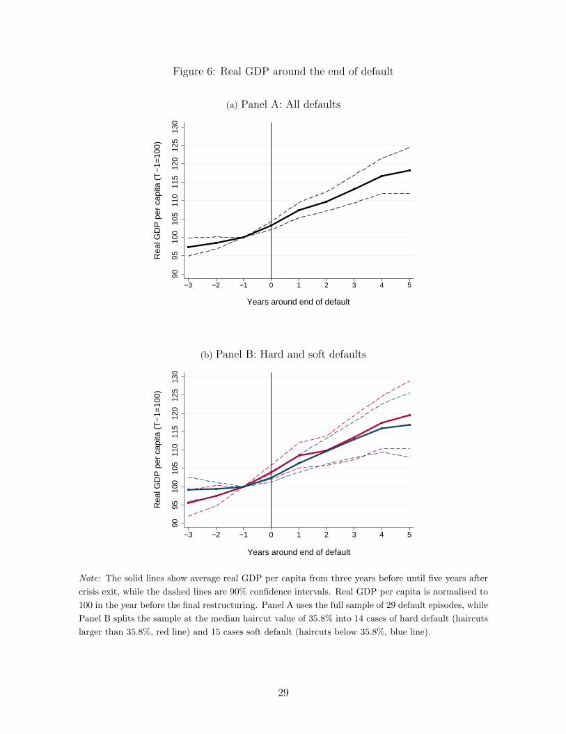
Figure 6: Real GDP around the end of default

(a) Panel A: All defaults

9095

100

105

110

115

120

125

130

Rea

l GD

P p

er c

apita

(T

−1=

100)

−3 −2 −1 0 1 2 3 4 5

Years around end of default

(b) Panel B: Hard and soft defaults

9095

100

105

110

115

120

125

130

Rea

l GD

P p

er c

apita

(T

−1=

100)

−3 −2 −1 0 1 2 3 4 5

Years around end of default

Note: The solid lines show average real GDP per capita from three years before until five years after

crisis exit, while the dashed lines are 90% confidence intervals. Real GDP per capita is normalised to

100 in the year before the final restructuring. Panel A uses the full sample of 29 default episodes, while

Panel B splits the sample at the median haircut value of 35.8% into 14 cases of hard default (haircuts

larger than 35.8%, red line) and 15 cases soft default (haircuts below 35.8%, blue line).

29

explains the insignificant haircut coefficient after default? This is all the more surpris-

ing, since it stands in contrast to the highly significant coerciveness coefficients during

default.

One possibility is that only coerciveness affects growth while haircuts do not. How-

ever, the results in Column 7 of Table A.4 show that also the lagged (average) coer-

civeness index is insignificant post-default. The same is true if we inspect the data

graphically, analogous to Panel B, but using the average coerciveness index of the cri-

sis to define soft and hard defaulters. Average post-crisis growth is again remarkably

similar for the two sub-groups. Hence, in contrast to our result during crises, we do

not find direct evidence that the severity of a crisis matters for post-default growth.

Another potential explanation for the insignificant findings is that developing coun-

tries benefit from the debt relief effect of high haircuts, as concluded by Arslanalp and

Henry (2005) and Reinhart and Trebesch (2016a), thus mitigating any negative repu-

tational effects that high creditor losses could entail. Another interpretation is that the

size of the final haircut does not come as a surprise but has already been anticipated

by markets in the run up to the restructuring. Any negative effects of high haircuts on

growth would materialize earlier, during the often lengthy renegotiation period. This

latter explanation is analogous to Levy-Yeyati and Panizza (2011): defaults might be

particularly costly in the early phase of distress, when creditors start reacting to the

(expected) crisis and the potential losses on their debt holdings. Once these losses have

realized, however, and once the formal act of debt restructuring occurs, few additional

costs arise.

The results in this section should not be misinterpreted. In particular, they do not

imply that imposing high haircuts has no long-lasting effects on growth. As we have

explained, identification is difficult and there are competing channels, which are hard

to disentangle in the data at hand. Moreover, it is possible that the timing of the

restructuring is endogenous, and this may bias the haircut coefficient towards zero.

Indeed, both sovereigns and creditors may have an incentive to settle in good times,

when default risk is low and growth prospects are good (as shown in the models by Bi,

2008; Benjamin and Wright, 2009). The insignificant result post-default also does not

mean that there are no long-term costs of default. As we have shown, defaults can take

up to 10 years to resolve. Lower growth numbers for such an extended period can have

substantial cumulative wealth effects.

Finally, we should emphasize that the results in this analysis stand in contrast to

Cruces and Trebesch (2013). Here, we do not find that high haircuts are followed by

30

lower growth in the post-default period, while Cruces and Trebesch (2013) document

that higher haircuts are associated with higher sovereign bond yields later on and

delayed reaccess to international capital markets. One explanation for these disparate

results is the phenomenon of “Phoenix miracles” descibed by (Calvo et al., 2006).

Emerging markets often see a quick recovery of output after financial crises, even if

credit and capital flows remain depressed and market access is unfavorable.

6 Conclusion

In this paper, we move beyond the classic dichotomous treatment of sovereign defaults

and use continuous measures on government payment and negotiation behavior and the

size of creditor losses in debt crises. We show that coercive actions towards external

creditors are associated with a much steeper drop in output when compared to cases

with consensual crisis resolution.

On average, “hard” defaults are associated with a 2 to 4 percentage points lower

growth rate during the crisis, depending on the sample and estimation method. Surpris-

ingly however, we do not find that high haircuts and debtor coerciveness are associated

with lower growth in the post-crisis period. The cost of “hard” defaults thus seems to

be most relevant during debt crisis episodes (which can take many years) but not so

much afterwards.

Our results support the view that the cost of debt crises depend to an important

degree on the severity of default and not only on its occurrence. This is in line with

Aguiar and Amador (2014) who discuss why it is important to consider “richer notions

of default”. More generally, the results can be interpreted as evidence for the existence

of a tradeoff: coercive debtor policies and high haircuts may have social and political

benefits in the short-run, but they also imply lower growth in the course of the crisis,

thus delaying recovery.

31

References

Abbas, S. M. A., N. Belhocine, A. A. ElGanainy, and M. A. Horton (2010):

“A Historical Public Debt Database,” IMF Working Paper 10/245, International

Monetary Fund.

Adam, K. and M. Grill (2013): “Optimal Sovereign Default,” Discussion Paper

09/2013, Deutsche Bundesbank, Research Centre.

Aggarwal, V. K. (1996): Debt Games: Strategic Interaction in International Debt

Rescheduling, Cambridge University Press.

Aguiar, M. and M. Amador (2014): “Sovereign Debt,” in Handbook of Interna-

tional Economics, ed. by K. R. Elhanan Helpman and G. Gopinath, Elsevier, vol. 5,

chap. 11, 647–687.

Aguiar, M., M. Amador, E. Farhi, and G. Gopinath (2013): “Crisis and

Commitment: Inflation Credibility and the Vulnerability to Sovereign Debt Crises,”

NBER Working Paper 19516, National Bureau of Economic Research, Inc.

Aguiar, M. and G. Gopinath (2006): “Defaultable Debt, Interest Rates and the

Current Account,” Journal of International Economics, 69, 64–83.

Andritzky, J. (2006): Sovereign Default Risk Valuation: Implications of Debt Crises

and Bond Restructurings, Springer.

Arellano, C. (2008): “Default Risk and Income Fluctuations in Emerging

Economies,” American Economic Review, 98, 690–712.

Arellano, C., X. Mateos-Planas, and J.-V. Rıos-Rull (2013): “Partial De-

fault,” Mimeo, NBER.

Arellano, C. and A. Ramanarayanan (2012): “Default and the Maturity Struc-

ture in Sovereign Bonds,” Journal of Political Economy, 120, 187 – 232.

Arslanalp, S. and P. B. Henry (2005): “Is Debt Relief Efficient?” Journal of

Finance, 60, 1017–1051.

Arteta, C. and G. Hale (2008): “Sovereign Debt Crises and Credit to the Private

Sector,” Journal of International Economics, 74, 53–69.

Asonuma, T. and C. Trebesch (2016): “Sovereign Debt Restructurings: Preemp-

tive Or Post-Default,” Journal of the European Economic Association, 14, 175–214.

32

Barro, R. J. (1977): “Unanticipated Money Growth and Unemployment in the

United States,” American Economic Review, 67, 101–15.

Barro, R. J. and J.-W. Lee (2010): “A New Data Set of Educational Attainment in

the World, 1950 - 2010,” NBER Working Paper 15902, National Bureau of Economic

Research, Inc.

Beck, N. and J. N. Katz (2011): “Modeling Dynamics in Time-Series-Cross-Section

Political Economy Data,” Annual Review of Political Science, 14, 331–352.

Benjamin, D. and M. L. J. Wright (2009): “Recovery Before Redemption: A

Theory Of Delays In Sovereign Debt Renegotiations,” CAMA Working Paper 2009-

15, Australian National University, Centre for Applied Macroeconomic Analysis.

Bi, R. (2008): “Beneficial Delays in Debt Restructuring Negotiations,” IMF Working

Papers 08/38, International Monetary Fund.

Bocola, L. (2015): “The Pass-Through of Sovereign Risk,” Working Papers 722,

Federal Reserve Bank of Minneapolis.

Bolton, P. and O. Jeanne (2007): “Structuring and Restructuring Sovereign Debt:

The Role of a Bankruptcy Regime,” Journal of Political Economy, 115, 901–924.

——— (2011): “Sovereign Default Risk and Bank Fragility in Financially Integrated

Economies,” IMF Economic Review, 59, 162–194.

Borensztein, E. and U. Panizza (2009): “The Costs of Sovereign Default,” IMF

Staff Paper, 56, 683–741.

Brambor, T., W. R. Clark, and M. Golder (2006): “Understanding interaction

models: improving empirical analyses,” Political Analysis, 14(1).

Bulow, J. and K. Rogoff (1989): “Sovereign Debt: Is to Forgive to Forget?”

American Economic Review, 79, 43–50.

Calvo, G. A. (1988): “Servicing the Public Debt: The Role of Expectations,” Amer-

ican Economic Review, 78, 647–61.

Calvo, G. A., A. Izquierdo, and E. Talvi (2006): “Sudden Stops and Phoenix

Miracles in Emerging Markets.” American Economic Review, 96(2), 405–410.

Cameron, C. A. and P. K. Tivedi (2005): Microeconometrics, Methods and Appli-

cations, Cambridge University Press.

33

Catao, L. and R. Mano (2015): “Default Premium,” IMF Working Papers 15/167,

International Monetary Fund.

Chatterjee, S. and B. Eyigungor (2012): “Maturity, Indebtedness, and Default

Risk,” American Economic Review, 102, 2674–99.

Cline, W. R. (1995): International Debt Reexamined, 46, Washington D.C.: Peterson

Institute for International Economics.

——— (2004): “Private Sector Involvement in Financial Crisis Resolution: Definition,

Measurement, and Implementation.” in Fixing Financial Crises in the Twenty-first

Century, ed. by A. Haldane, Routledge, 61–94.

Cole, H., D. Neuhann, and G. Ordonez (2016): “Debt Crises: For Whom the

Bell Tolls,” NBER Working Papers 22330, National Bureau of Economic Research,

Inc.

Cole, H. L. and P. J. Kehoe (1997): “Reviving Reputation Models of International

Debt,” Quarterly Review, 21, 21–30.

——— (1998): “Models of Sovereign Debt: Partial versus General Reputations,” In-

ternational Economic Review, 39, 55–70.

Corsetti, G. and L. Dedola (2012): “The Mystery of the Printing Press: Self-

fulfilling Debt Crises and Monetary Sovereignty,” CEPR Discussion Paper No. 9358.

Cruces, J. J. and C. Trebesch (2013): “Sovereign Defaults: The Price of Hair-

cuts,” American Economic Journal: Macroeconomics, 5, 85–117.

De Paoli, B., G. Hoggarth, and V. Saporta (2009): “Output Costs of Sovereign

Crises: Some Empirical Estimates,” Bank of England Working Paper 362, Bank of

England.

D’Erasmo, P. and E. G. Mendoza (2016): “Distributional Incentives In An Equi-

librium Model Of Domestic Sovereign Default,” Journal of the European Economic

Association, 14, 7–44.

Dubey, P., J. Geanakoplos, and M. Shubik (2005): “Default and Punishment

in General Equilibrium,” Econometrica, 73, 1–37.

Eaton, J. and R. Fernandez (1995): “Sovereign debt,” in Handbook of Interna-

tional Economics, ed. by G. M. Grossman and K. Rogoff, Elsevier, vol. 3, chap. 3,

2031–2077.

34

Eaton, J. and M. Gersovitz (1981): “Debt with Potential Repudiation: Theoreti-

cal and Empirical Analysis,” Review of Economic Studies, 48, 289–309.

Eichengreen, B. (1991): “Historical Research on International Lending and Debt,”

The Journal of Economic Perspectives, 5, 149–169.

Enderlein, H., C. Trebesch, and L. von Daniels (2012): “Sovereign Debt

Disputes: A Database on Government Coerciveness during Debt Crises,” Journal of

International Money and Finance, 31, 250–266.

Furceri, D. and A. Zdzienicka (2012): “How Costly are Debt Crises?” Journal of

International Money and Finance, 31, 726–742.

Gennaioli, N., A. Martin, and S. Rossi (2014a): “Banks, Government Bonds,

and Default: What do the Data Say?” CEPR Discussion Paper 10044, C.E.P.R.

Discussion Paper.

——— (2014b): “Sovereign Default, Domestic Banks, and Financial Institutions,”

Journal of Finance, 69, 819–866.

Goldberger, A. S. (1991): A Course in Econometrics, Harvard University Press.

Gornemann, N. M. (2016): “Sovereign Default, Private Investment, and Economic

Growth,” Journal of the European Economic Association, 14, 215–251.

Grossman, H. and J. van Huyck (1988): “Sovereign Debt as a Contingent Claim:

Excusable Default, Repudiation, and Reputation,” American Economic Review, 78,

1088–1097.

Hardin, J. W. (2002): “The Robust Variance Estimator for Two-Stage Models,”

Stata Journal, 2, 253–266.

Hatchondo, J. C. and L. Martinez (2012): “Debt Dilution and Sovereign Default

Risk,” Working Paper 10-08, Federal Reserve Bank of Richmond.

Hatchondo, J. C., L. Martinez, and C. Sosa Padilla (2014): “Voluntary

sovereign debt exchanges,” Journal of Monetary Economics, 61, 32–50.

Hebert, B. and J. Schreger (2016): “The Costs of Sovereign Default: Evidence

from Argentina,” NBER Working Papers 22270, National Bureau of Economic Re-

search, Inc.

35

Hole, A. R. (2006): “Calculating Murphy-Topel Variance Estimates in Stata: A

Simplified Procedure,” Stata Journal, 6, 521–529.

Hurwicz, L. (1950): “Least Square Bias in Time Series,” in Statistical Inference in

Dynamic Economic Models, ed. by T. C. Koopmans, Wiley, chap. XV, 365–383.

Institute of International Finance (2013): “Principles for Stable Capital Flows

and Fair Debt Restructuring, Report on Implementation by the Principles Consulta-

tive Group,” Institute of International Finance.

International Monetary Fund (1999): IMF Policy on Lending into Arrears to

Private Creditors, International Monetary Fund.

——— (2002): Fund Policy on Lending into Arrears to Private Creditors - Further

Consideration of the Good Faith Criterion, International Monetary Fund.

Judson, R. A. and A. L. Owen (1999): “Estimating Dynamic Panel Data Models:

A Guide for Macroeconomists,” Economics Letters, 65, 9–15.

Kennedy, P. (2003): A Guide to EconometricsA Guide to Econometrics, MIT Press,

5 ed.

Kletzer, K. M. and B. D. Wright (2000): “Sovereign Debt as Intertemporal

Barter,” American Economic Review, 90, 621–639.

Kuvshinov, D. and K. Zimmermann (2016): “Sovereigns going

bust: estimating the cost of default,” Bonn Econ Discussion Papers

bgse012016, UniversityofBonn,Germany.

Laeven, L. and F. Valencia (2012): “Systemic Banking Crises Database: An Up-

date,” IMF Working Paper 12/163, International Monetary Fund.

Levy-Yeyati, E. and U. Panizza (2011): “The Elusive Costs of Sovereign Defaults,”

Journal of Development Economics, 94, 95–105.

Marchesi, S. (2016): “Life after default? Private vs. official sovereign debt restructur-

ings,” Development Working Papers 398, Centro Studi Luca d’Agliano, University of

Milano.

Mendoza, E. G. and V. Z. Yue (2012): “A General Equilibrium Model of Sovereign

Default and Business Cycles,” The Quarterly Journal of Economics, 127, 889–946.

36

Murphy, K. M. and R. H. Topel (1985): “Estimation and Inference in Two-Step

Econometric Models,” Journal of Business & Economic Statistics, 3, 370–79.

Nickell, S. J. (1981): “Biases in Dynamic Models with Fixed Effects,” Econometrica,

49, 1417–26.

Obstfeld, M. and A. M. Taylor (2003): “Sovereign Risk, Credibility and the Gold

Standard: 1870-1913 versus 1925-31,” Economic Journal, 113, 241–275.

Panizza, U., F. Sturzenegger, and J. Zettelmeyer (2009): “The Economics and

Law of Sovereign Debt and Default,” Journal of Economic Literature, 47, 651–98.

Reinhart, C. M., V. R. Reinhart, and K. S. Rogoff (2012): “Public Debt Over-

hangs: Advanced-Economy Episodes since 1800,” Journal of Economic Perspectives,

26, 69–86.

Reinhart, C. M., K. S. Rogoff, and M. A. Savastano (2003): “Debt Intolerance,”

Brookings Paper on Economic Activity, 34, 1–74.

Reinhart, C. M. and C. Trebesch (2016a): “Sovereign Debt Relief And Its After-

math,” Journal of the European Economic Association, 14, 215–251.

——— (2016b): “The International Monetary Fund: 70 Years of Reinvention,” Journal

of Economic Perspectives, 30, 3–28.

Rose, A. K. (2005): “One reason countries pay their debts: renegotiation and interna-

tional trade,” Journal of Development Economics, 77, 189–206.

Roubini, N. (2004): “Private Sector Involvement in Crisis Resolution and Mechanisms

for Dealing with Sovereign Debt Problems.” in Fixing Financial Crises in the Twenty-

first Century, ed. by A. Haldane, Routledge, 61–94.

Roubini, N. and B. Setser (2004): Bailouts or Bail-ins? Responding to Financial

Crises in Emerging Economies, no. 378 in Peterson Institute Press: All Books, Peterson

Institute for International Economics.

Sandleris, G. (2008): “Sovereign Defaults: Information, Investment and Credit,” Jour-

nal of International Economics, 76, 267 – 275.

Sandleris, G. and M. L. J. Wright (2014): “The Costs of Financial Crises: Resource

Misallocation, Productivity, and Welfare in the 2001 Argentine Crisis,” Scandinavian

Journal of Economics, 116, 87–127.

37

Standard & Poor’s (2011): “Sovereign Defaults and Rating Transition Data: 2010

Update,” Ratingsdirect, Standard & Poor’s.

Sturzenegger, F. (2004): “Tools for the Analysis of Debt Problems,” Journal of Re-

structuring Finance, 01, 201–223.

Sturzenegger, F. and J. Zettelmeyer (2007): Debt Defaults and Lessons from a

Decade of Crises, The MIT Press.

——— (2008): “Haircuts: Estimating Investor Losses in Sovereign Debt Restructurings,

1998-2005,” Journal of International Money and Finance, 27, 780–805.

Tomz, M. and M. L. Wright (2013): “Empirical Research on Sovereign Debt and

Default,” Annual Review of Economics, 5, 247–272.

Tomz, M. and M. L. J. Wright (2007): “Do Countries Default in ”Bad Times”?”

Journal of the European Economic Association, 5, 352–360.

Trebesch, C. (2009): “The Cost of Aggressive Sovereign Debt Policies: How Much

is the Private Sector Affected?” IMF Working Paper 09/29, International Monetary

Fund.

Wright, M. L. J. (2002): “Reputation and Sovereign Debt,” Working Paper.

Yue, V. Z. (2010): “Sovereign Default and Debt Renegotiation,” Journal of International

Economics, 80, 176–187.

Zame, W. R. (1993): “Efficiency and the Role of Default When Security Markets Are

Incomplete,” American Economic Review, 83, 1142–1164.

38

Online Appendix

39

Figure A.1: Coerciveness index: descriptive statistics

(a) Distribution of coerciveness index

010

2030

40

Num

ber

of a

nnua

l obs

erva

tions

1 2 3 4 5 6 7 8 9

Value of coerciveness index

(b) Summary statistics on the coerciveness indexand its subindicators

Variable Frequency Min Max

Coerciveness index 217 0 9

Payments missed 157 0 1

Unilateral suspension 128 0 1

Full suspension 56 0 1

Freeze on assets 27 0 1

Negotiations breakdown 97 0 1

Moratorium declaration 28 0 1

Threats to repudiate 38 0 1

Data disputes 21 0 1

Forced restructuring 13 0 1

40

Figure A.2: Haircuts: descriptive statistics

(a) Size of haircuts across countries and time

Turkey

Romania

Mexico

VenezuelaMorocco

Chile

Costa Rica

Nigeria

UruguayPhilippines

Argentina

South Africa

Jordan

Brazil

Bulgaria

Dominican RepublicPoland

Albania

Ecuador

Algeria

Panama

Peru

Pakistan

Ecuador

Ukraine

Russia

Uruguay

Dominican Republic

Argentina

Ecuador

020

4060

80H

airc

ut in

%

1980 1985 1990 1995 2000 2005 2009Year

(b) Descriptive statistics

# of obs. Min. Max. Mean Median Std. Dev.

Haircuts 30 5% 80% 38% 36% 21%

41

Figure A.3: Government coerciveness and crisis duration

(a) Panel A: Level of debtor coerciveness and default dura-tion

01

23

45

Ave

rage

val

ue o

f the

coe

rciv

enes

s in

dex

1 2 3 4 5 6 7 8 9 10 11 12 13 14 15

Duration of debt crisis (in years)

(b) Panel B: Changes in debtor coerciveness and default du-ration

−4

−3

−2

−1

01

2

Cha

nge

in c

oerc

iven

ess

inde

x (y

oy)

0 1 2 3 4 5 6 7 8 9 10 11 12 13 14 15

Duration of debt crisis (in years)

Note: Panel A shows the average coerciveness index value for each debt crisis year. In the first year

of default the coerciveness index has an average value of 3.2, in the second year 3.6, and so on. Panel

B shows average year-on-year changes in the coerciveness index, starting from the second year of a

debt crisis. The dashed lines indicate 90% confidence intervals. Note that the number of observations

declines notably in default duration. For example the 15th year of default is observed just once (Peru

1997), while there are only three observations in the 14th default year (Peru, Panama and Ecuador).

42

Table A.1: Country sample and debt crisis years

List of defaulters (25 countries), with years of debt crisis

Albania: 1980-2009 (1991-1995) Pakistan: 1980-2009 (1998-1999)Algeria: 1980-2009 (1991-1996) Panama: 1980-2009 (1983-1996)Argentina: 1980-2009 (1982-1993; Peru: 1981-2009 (1983-1997)2001-2005)Brazil: 1980-2009 (1983-1994) Philippines: 1980-2009 (1983-1992)Bulgaria: 1980-2009 (1990-1994) Poland: 1991-2009 (1991-1994)Chile: 1980-2009 (1983-1990) Romania: 1980-2009 (1981-1983; 1986)Costa Rica: 1980-2009 (1981-1990) Russia: 1989-2009 (1991-2000)Dominican Republic: 1980-2009 (1982- South Africa: 1980-2009 (1985-1987;1994; 2004-2005) 1989;1993)Ecuador: 1980-2009 (1982-1995; 1999- Turkey: 1980-2009 (1981-1982)2000; 2008-2009)Jordan: 1980-2009 (1989-1993) Ukraine: 1987-2009 (1998-2000)Mexico: 1980-2009 (1982-1990) Uruguay: 1980-2009 (1983-1991; 2003)Morocco: 1980-2009 (1983-1990) Venezuela: 1980-2009 (1982-1990;

2004-2005)Nigeria: 1980-2000 (1982-1992)

List of non-defaulter (36 countries)

Armenia: 1995-2009 Lithuania: 1990-2009Azerbaijan: 1995-2009 Malaysia: 1980-2009Bahrain: 1980-2009 Mauritius: 1980-2009Belarus: 1990-2009 Namibia: 1980-2009Botswana: 1980-2009 Oman: 1980-2009China: 1980-2009 Papua New Guinea: 1980-2009Colombia: 1980-2009 Puerto Rico: 1980-2009Egypt: 1980-2009 Qatar: 1995-2009El Salvador: 1980-2009 Saudi Arabia: 1980-2009Georgia: 1980-2009 Singapore: 1980-2009Hong Kong: 1980-2009 Slovak Republic: 1984-2009Hungary: 1980-2009 Swaziland: 1980-2009India: 1980-2009 Syria: 1980-2009Kazakhstan: 1990-2009 Thailand: 1980-2009Kuwait: 1995-2009 Tunisia: 1980-2009Latvia: 1980-2009 Turkmenistan: 1987-2009Lebanon: 1992-2009 United Arab Emirates: 1980-2009Libya: 1999-2009 Uzbekistan: 1987-2009

43

Table A.2: Variable definitions

Variable Definition Sources

Growth Annual growth rate of real GDP per capita (in per-cent)

World Development Indi-cators

Default Dummy variable taking on a value of one for eachyear a country has been listed as being in default byStandard & Poor’s

Standard & Poor’s

Inv/GDP Investment to GDP ratio World Development Indi-cators

∆Pop Annual growth rate of population (in percent) World Development Indi-cators

Log(Pop) Natural logarithm of total population (in million) World Development Indi-cators

SecEdu Share of population that attained secondary schooling(in percent)

Barro and Lee (2010)

GovtConst−1 Lagged annual growth rate of government consump-tion expenditure (in percent)

World Development Indi-cators

CivLib Annual index value of the civil liberties index pub-lished by Freedom House in its annual Freedom in theWorld report. The index ranges from 1 (highest de-gree of freedom) to 7 (lowest degree of freedom)

Freedom House Freedomin the World

∆ToT Annual rate of change in current price value of exportsof goods and services deflated by the import price in-dex (exports as capacity to import)

World Development Indi-cators

Openness Ratio of average exports plus imports (=Exports+Imports

2 ) to GDP (in percent)World Development Indi-cators

BankingCrisis Dummy variable with a value of one at the beginningof a banking crisis

Laeven and Valencia(2012)

PoliticalRisk

ICRG Political Risk Index, ranging from a minimumof 0 to a maximum of 100

Political Risk Group

GovChange Dummy variable with a value of one in years with achange in the executive

Database of Political In-stitutions (DPI) 2012

CurrencyCrisis Dummy variable with a value of one at the beginningof a currency crisis

Laeven and Valencia(2012)

Debt/GDP Ratio of government debt to GDP (in percent) Abbas et al. (2010)

Ratings Institutional Investor’s Country Credit Rating issuedat the start of each year. The credit rating scaleranges from zero (extremely high credit risk) to 100(extremely low credit risk)

Institutional InvestorMagazine

IMFt−1 Dummy variable with a value of one in case of anongoing IMF program

Reinhart and Trebesch(2016b)

44

Table A.3: Summary statistics - main variables

Variable Mean Std. Dev. Min Max

Growth 2.03884 5.774445 -45.32511 33.03048

Coerc 0.4727932 1.410846 0 9

Haircut 37.92333 20.67408 4.7 80.4

Default 0.1269649 0.3330344 0 1

Inv/GDP 0.2399193 0.0751849 0.02388 0.72408

∆Pop 1.727398 1.885407 -2.62465 20.42816

Log(Pop) 2.457494 1.644205 -1.027342 7.193971

SecEdu 46.93156 20.18757 9.599999 93.49851

GovtConst−1 3.842325 7.82335 -44.84714 83.22173

CivLib 3.990903 1.618302 1 7

∆ToT 0.0676785 0.1579326 -0.7147055 1.122298

Openness 88.8763 62.82052 11.54567 460.4711

BankingCrisis 0.036208 0.1868689 0 1

Political Risk 64.26955 10.82045 29.5 89.12

GovChange 0.1580328 0.3648914 0 1

CurrencyCrisis 0.041717 0.2000023 0 1

Debt/GDP 51.46241 36.4501 0 289.6

Ratings 41.97108 17.4068 6.4 93.1

IMFt−1 0.3345888 0.4719947 0 1

45

Table A.4: Haircuts, coerciveness, and post-default GDP growth

(1) (2) (3) (4) (5) (6)Plain I Plain II Macro Country FE Addition. Average

Controls Controls Coerc

Haircut 0.0255*** 0.0315* -0.0218 -0.0195 -0.0223(5yr lag) (0.0089) (0.0179) (0.0142) (0.0184) (0.0143)Default -0.3056 1.4767** 1.4866* 0.6421 0.8809(5yr lag) (0.7332) (0.6371) (0.8668) (0.6912) (0.6296)IMFt−1 0.4873(Dummy) (0.3505)Coerc -0.0791(5yr lag) (0.1360)Inv/GDP 17.8510*** 19.3975*** 23.3745*** 17.7085***

(1.9699) (3.3316) (3.6779) (1.9629)∆Pop -0.4058** -0.0595 -1.2373*** -0.3985**

(0.1698) (0.4140) (0.3206) (0.1709)Log(Pop) -0.0516 0.9431 7.4477*** -0.0378

(0.0853) (3.2905) (2.7948) (0.0855)SecEdu 0.0300*** 0.0385 0.0458 0.0294***

(0.0086) ((0.0507) (0.0380) (0.0086)GovtConst−1 0.1005*** 0.0896*** 0.0797*** 0.0975***

(0.0216) (0.0222) (0.0262) (0.0219)CivLib 0.0318 0.1071 0.0634 0.0271

(0.1014) (0.2745) (0.2354) (0.1021)∆ToT 9.5672*** 9.8570*** 8.7619*** 9.4561***

(1.4157) (1.6596) (1.1828) (1.4208)Openness -0.0028 -0.0091 0.0238*** -0.0026

(0.0024) (0.0160) (0.0092) (0.0024)BankingCrisis -2.7434*** -2.6657*** -2.7849*** -2.7649***(Dummy) (0.7915) (0.6882) (0.8818) (0.7904)Political Risk 0.0397

(0.0298)GovChange -0.8924**(Dummy) (0.3703)CurrencyCrisis -4.8892***(Dummy) (1.2392)Debt/GDP 0.0252*

(0.0139)

Observations 1,347 1,347 887 887 724 887Countries 61 61 45 45 45 45Time FE YES YES YES YES YES YESCountry FE NO NO NO YES YES YESR2 0.1281 0.1282 0.3939 0.3475 0.4444 0.3925

Note: The dependent variable is the annual growth rate of real GDP per capita, measured in percentage

points. The key explanatory variable is the haircut of the final restructuring, which is carried forward

for five years after crisis exit (column 1-5). In column 6, we use the average coerciveness index value

over the whole default episode, also lagged for the subsequent five years. All specifications include

a (non-reported) constant. Robust standard errors are given in parentheses. ***, **, and * denote

significance at the 1, 5, and 10 per cent levels, respectively.

46