Housing supply and price reaction: A comparative approach between Spanish and

Italian markets

Laura GabrielliPaloma Taltavull

Agenda• Introduction: housing supply evolution and

the role on the economies of Italy and Spain• Cicles comparison• Housing supply estimation• Conclusions

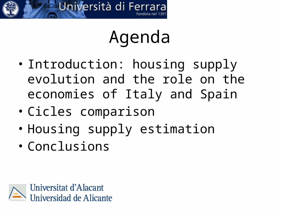
Construction sector in Italian Economy• GDP includes investment in constructions (residential, non residential and

civil engineering works), transaction costs and rents and housing services• In 2010 this sector represented the 10,24% of GPD, with a strong reduction

in construction investments• Rents and imputed rents are growing: that figure overcame investment in

constructions in the last two yearsIstat; Conti economici annuall real value

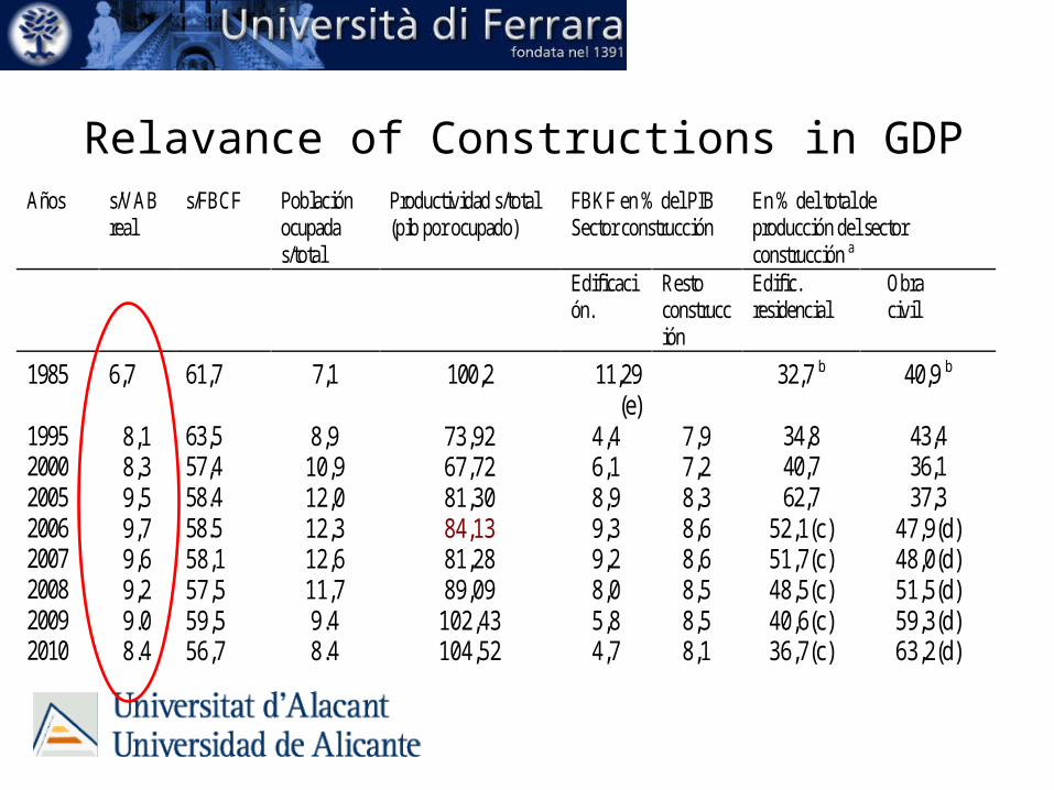
Relavance of Constructions in GDPAños s/VAB

real s/FBCF Población

ocupada s/total

Productividad s/total (pib por ocupado)

FBKF en % del PIB Sector construcción

En % del total de producción del sector construcción a

Edificación.

Resto construcción

Edific. residencial

Obra civil

1985 6,7 61,7 7,1 100,2 11,29 (e)

32,7 b 40,9 b

1995 8,1 63,5 8,9 73,92 4,4 7,9 34,8 43,4 2000 8,3 57,4 10,9 67,72 6,1 7,2 40,7 36,1 2005 9,5 58.4 12,0 81,30 8,9 8,3 62,7 37,3 2006 9,7 58.5 12,3 84,13 9,3 8,6 52,1(c) 47,9(d) 2007 9,6 58,1 12,6 81,28 9,2 8,6 51,7(c) 48,0(d) 2008 9,2 57,5 11,7 89,09 8,0 8,5 48,5(c) 51,5(d) 2009 9.0 59,5 9.4 102,43 5,8 8,5 40,6(c) 59,3(d) 2010 8.4 56,7 8.4 104,52 4,7 8,1 36,7(c) 63,2(d)

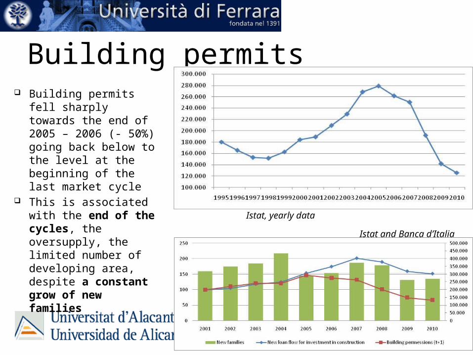
Building permits Building permits fell

sharply towards the end of 2005 – 2006 (- 50%) going back below to the level at the beginning of the last market cycle

This is associated with the end of the cycles, the oversupply, the limited number of developing area, despite a constant grow of new families

Istat, yearly data

Istat and Banca d’Italia

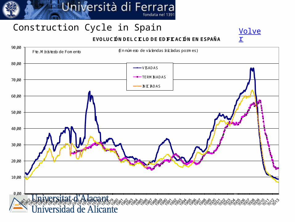
Construction Cycle in Spain Volver

0,00

10,00

20,00

30,00

40,00

50,00

60,00

70,00

80,00

90,00

EVOLUCIÓN DEL CICLO DE EDIFICACIÓN EN ESPAÑA

VISADAS

TERMINADAS

INICIADAS

(En número de viviendas iniciadas por mes)Fte. Ministerio de Fomento

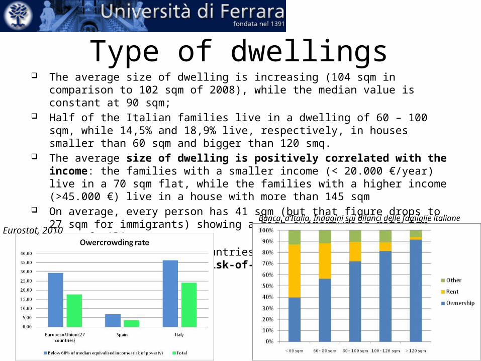
Type of dwellings The average size of dwelling is increasing (104 sqm in comparison to 102 sqm of 2008), while

the median value is constant at 90 sqm; Half of the Italian families live in a dwelling of 60 – 100 sqm, while 14,5% and 18,9% live,

respectively, in houses smaller than 60 sqm and bigger than 120 smq. The average size of dwelling is positively correlated with the income: the families with a

smaller income (< 20.000 €/year) live in a 70 sqm flat, while the families with a higher income (>45.000 €) live in a house with more than 145 sqm

On average, every person has 41 sqm (but that figure drops to 27 sqm for immigrants) showing a high overcrowding rate for those families

Spain is one of the Eu countries where the overcrowding rate among the population at-risk-of-poverty is below 6% (very low)

Eurostat, 2010Banca d’Italia, Indagini sui bilanci delle famiglie italiane

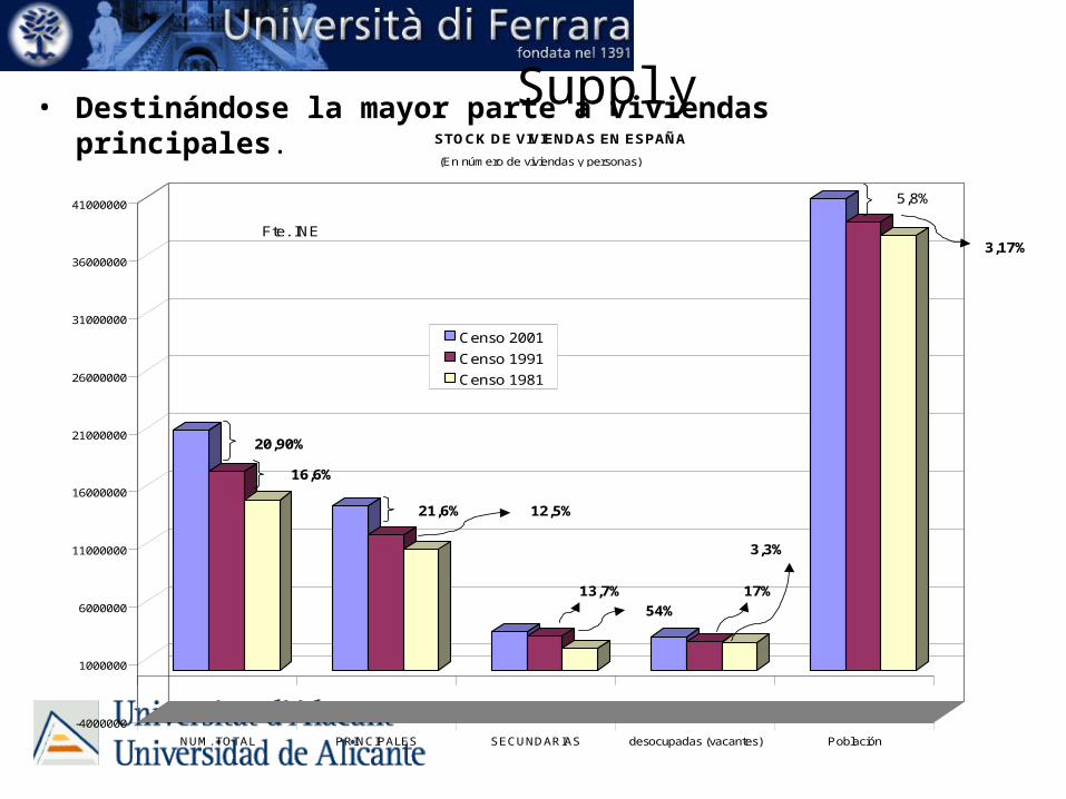
• Destinándose la mayor parte a viviendas principales. Supply

-4000000

1000000

6000000

11000000

16000000

21000000

26000000

31000000

36000000

41000000

NUM. TOTAL PRINCIPALES SECUNDARIAS desocupadas (vacantes) Población

STOCK DE VIVIENDAS EN ESPAÑA

Censo 2001

Censo 1991

Censo 1981

(En número de viviendas y personas)

Fte. INE

20,90%

13,7% 17%

5,8%

21,6%

3,17%

3,3%

54%

12,5%

16,6%

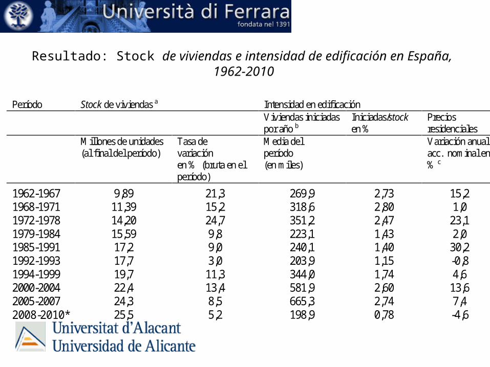
Resultado: Stock de viviendas e intensidad de edificación en España, 1962-2010

Período Stock de viviendas a Intensidad en edificación Viviendas iniciadas

por año b Iniciadas/stock en %

Precios residenciales

Millones de unidades (al final del período)

Tasa de variación en % (bruta en el período)

Media del período (en miles)

Variación anual acc. nominal en % c

1962-1967 9,89 21,3 269,9 2,73 15,2 1968-1971 11,39 15,2 318,6 2,80 1,0 1972-1978 14,20 24,7 351,2 2,47 23,1 1979-1984 15,59 9,8 223,1 1,43 2,0 1985-1991 17,2 9,0 240,1 1,40 30,2 1992-1993 17,7 3,0 203,9 1,15 -0,8 1994-1999 19,7 11,3 344,0 1,74 4,6 2000-2004 22,4 13,4 581,9 2,60 13,6 2005-2007 24,3 8,5 665,3 2,74 7,4 2008-2010* 25,5 5,2 198,9 0,78 -4,6

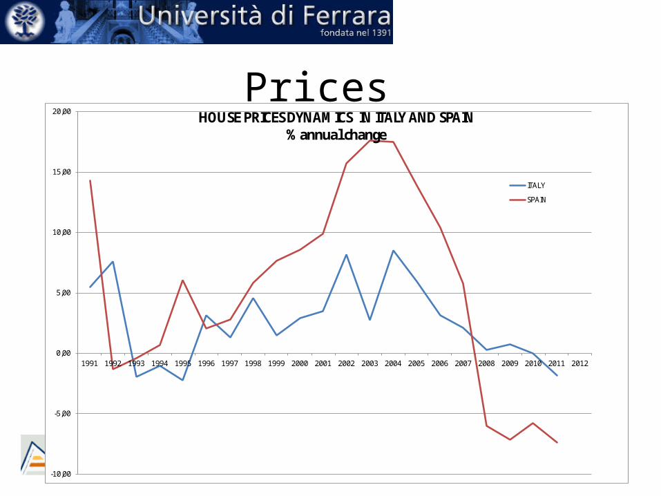
Prices

-10,00

-5,00

0,00

5,00

10,00

15,00

20,00

1991 1992 1993 1994 1995 1996 1997 1998 1999 2000 2001 2002 2003 2004 2005 2006 2007 2008 2009 2010 2011 2012

HOUSE PRICES DYNAMICS IN ITALY AND SPAIN% annual change

ITALY

SPAIN

Aim of this paper• Describe the housing cycle and price dynamics

in both countries• Approach the supply elasticity for comparison

purposes• Controlling by region

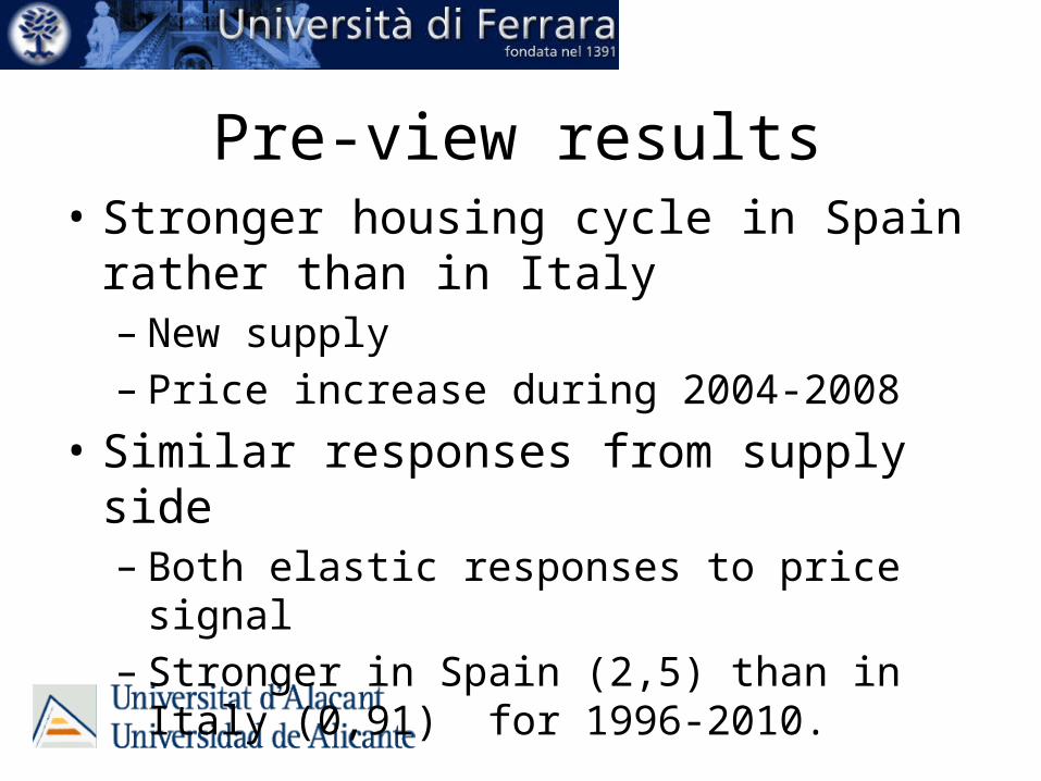
Pre-view results• Stronger housing cycle in Spain rather than in

Italy– New supply– Price increase during 2004-2008

• Similar responses from supply side– Both elastic responses to price signal– Stronger in Spain (2,5) than in Italy (0,91) for

1996-2010.

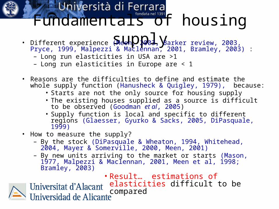
Fundamentals of housing supply• Different experience (Meen, 2003, Barker review, 2003, Pryce, 1999,

Malpezzi & Maclennan, 2001, Bramley, 2003) :– Long run elasticities in USA are >1– Long run elasticities in Europe are < 1

• Reasons are the difficulties to define and estimate the whole supply function (Hanusheck & Quigley, 1979), because:

• Starts are not the only source for housing supply• The existing houses supplied as a source is difficult to be observed

(Goodman et al, 2005) • Supply function is local and specific to different regions (Glaesser,

Gyurko & Sacks, 2005, DiPasquale, 1999) • How to measure the supply?

– By the stock (DiPasquale & Wheaton, 1994, Whitehead, 2004, Mayer & Somerville, 2000, Meen, 2001)

– By new units arriving to the market or starts (Mason, 1977, Malpezzi & Maclennan, 2001, Meen et al, 1998; Bramley, 2003)

• Result… estimations of elasticities difficult to be compared

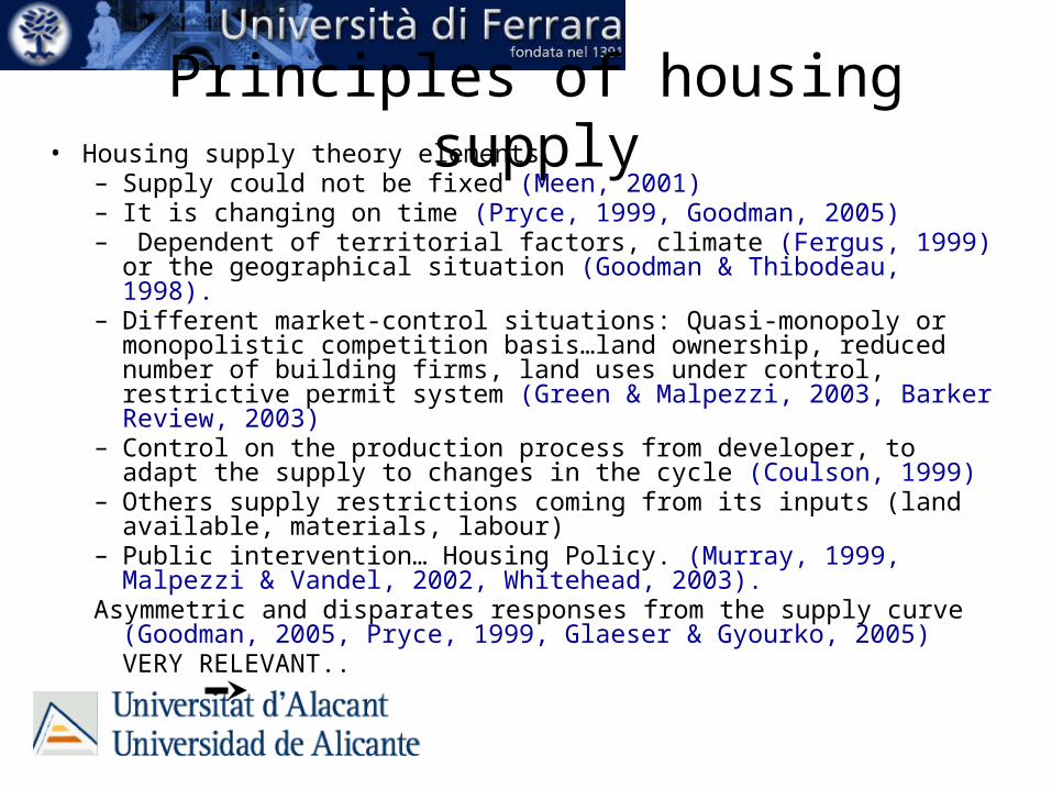
Principles of housing supply• Housing supply theory elements

– Supply could not be fixed (Meen, 2001)– It is changing on time (Pryce, 1999, Goodman, 2005) – Dependent of territorial factors, climate (Fergus, 1999) or the geographical

situation (Goodman & Thibodeau, 1998). – Different market-control situations: Quasi-monopoly or monopolistic

competition basis…land ownership, reduced number of building firms, land uses under control, restrictive permit system (Green & Malpezzi, 2003, Barker Review, 2003)

– Control on the production process from developer, to adapt the supply to changes in the cycle (Coulson, 1999)

– Others supply restrictions coming from its inputs (land available, materials, labour)

– Public intervention… Housing Policy. (Murray, 1999, Malpezzi & Vandel, 2002, Whitehead, 2003).

Asymmetric and disparates responses from the supply curve (Goodman, 2005, Pryce, 1999, Glaeser & Gyourko, 2005)

VERY RELEVANT..

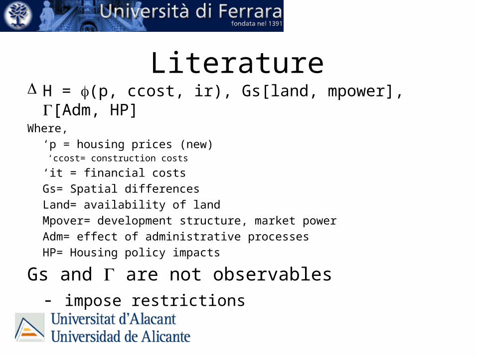
LiteratureD H = f(p, ccost, ir), Gs[land, mpower], G[Adm, HP]Where,

‘p = housing prices (new)‘ccost= construction costs

‘it = financial costsGs= Spatial differencesLand= availability of landMpover= development structure, market powerAdm= effect of administrative processesHP= Housing policy impacts

Gs and G are not observables- impose restrictions

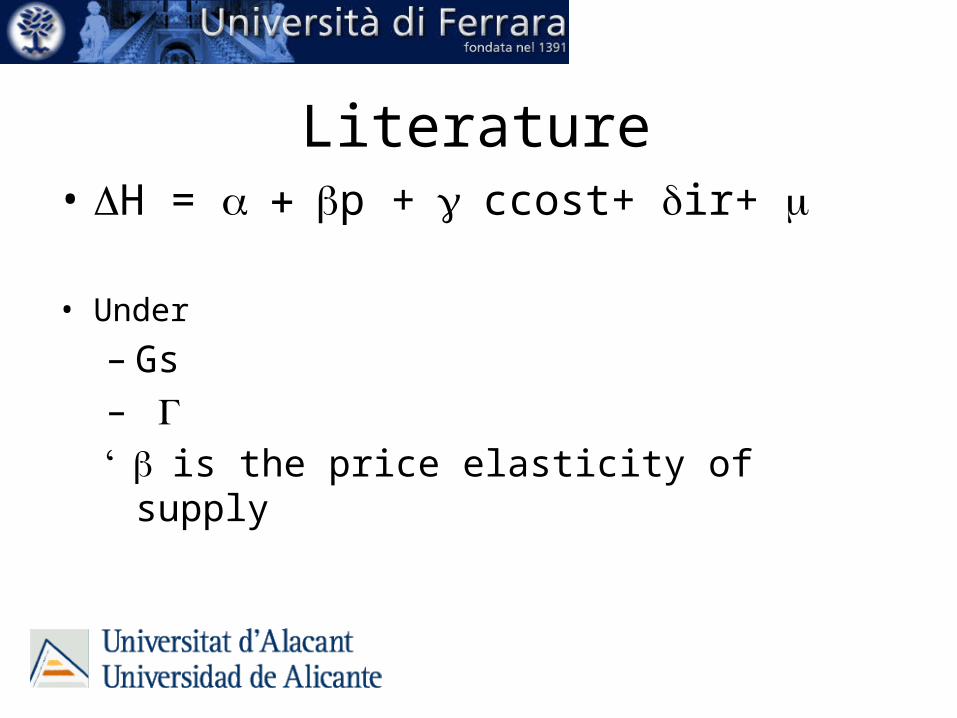
Literature• DH = + a bp + g ccost+ dir+ m

• Under

– Gs– G‘ b is the price elasticity of supply

17

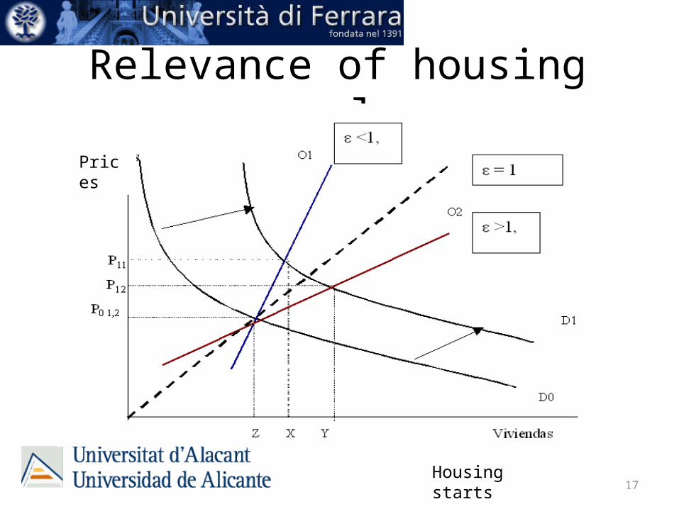
Relevance of housing supply…

Prices

Housing starts

18

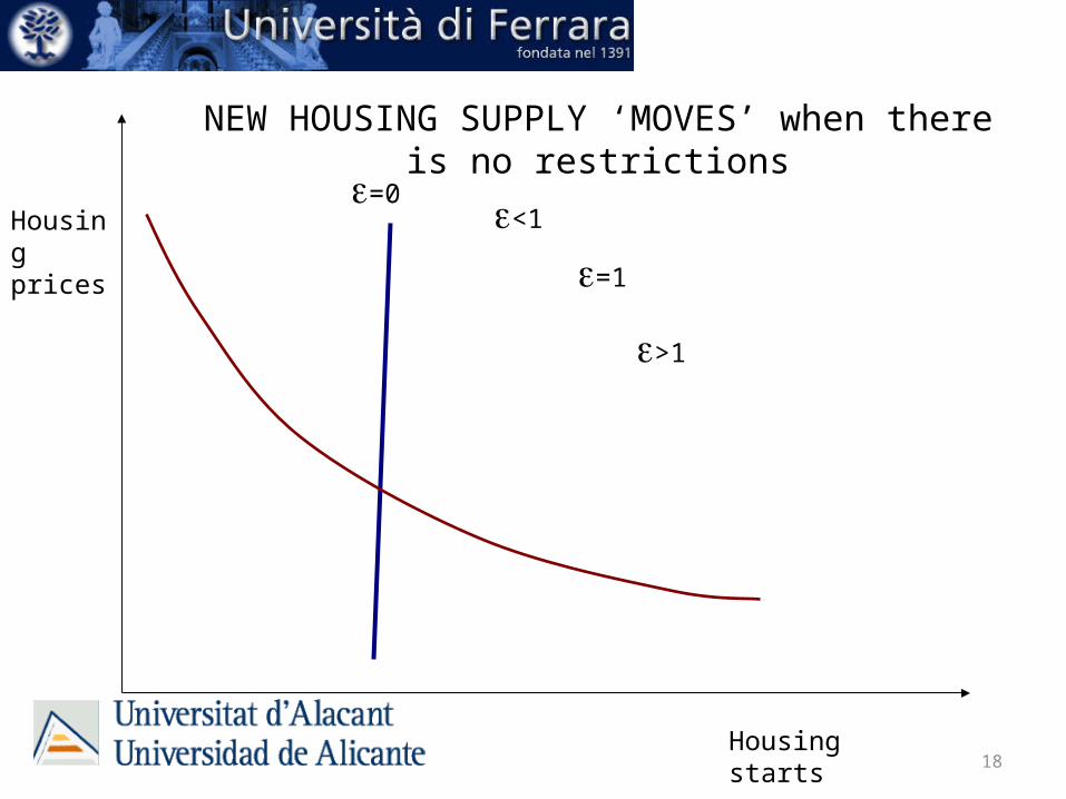
NEW HOUSING SUPPLY ‘MOVES’ when there is no restrictions

Housing starts

Housing prices

e<1e=0

e=1

e>1

Empirical analysis• Estimate housing supply elasticity of new

units• Market oriented focus:

• Prices are the signal… afecting starts

• Share of the market explained by the model• Theres is no ‘intervention’ on the market as:

– Market power– Escarcity of land– Administrative limits– Monopoly or oligopoly in development

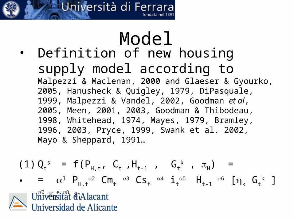
Model• Definition of new housing supply model

according to Malpezzi & Maclenan, 2000 and Glaeser & Gyourko, 2005, Hanusheck & Quigley, 1979, DiPasquale, 1999, Malpezzi & Vandel, 2002, Goodman et al, 2005, Meen, 2001, 2003, Goodman & Thibodeau, 1998, Whitehead, 1974, Mayes, 1979, Bramley, 1996, 2003, Pryce, 1999, Swank et al. 2002, Mayo & Sheppard, 1991…

(1) Qts = f(PH,t, Ct ,Ht-1 , Gt

k , pH) =

• = a1 PH,t2a Cmt 3a Cst 4a it

5a Ht-1 6a [hk Gtk ] 7a pH

e 8a et

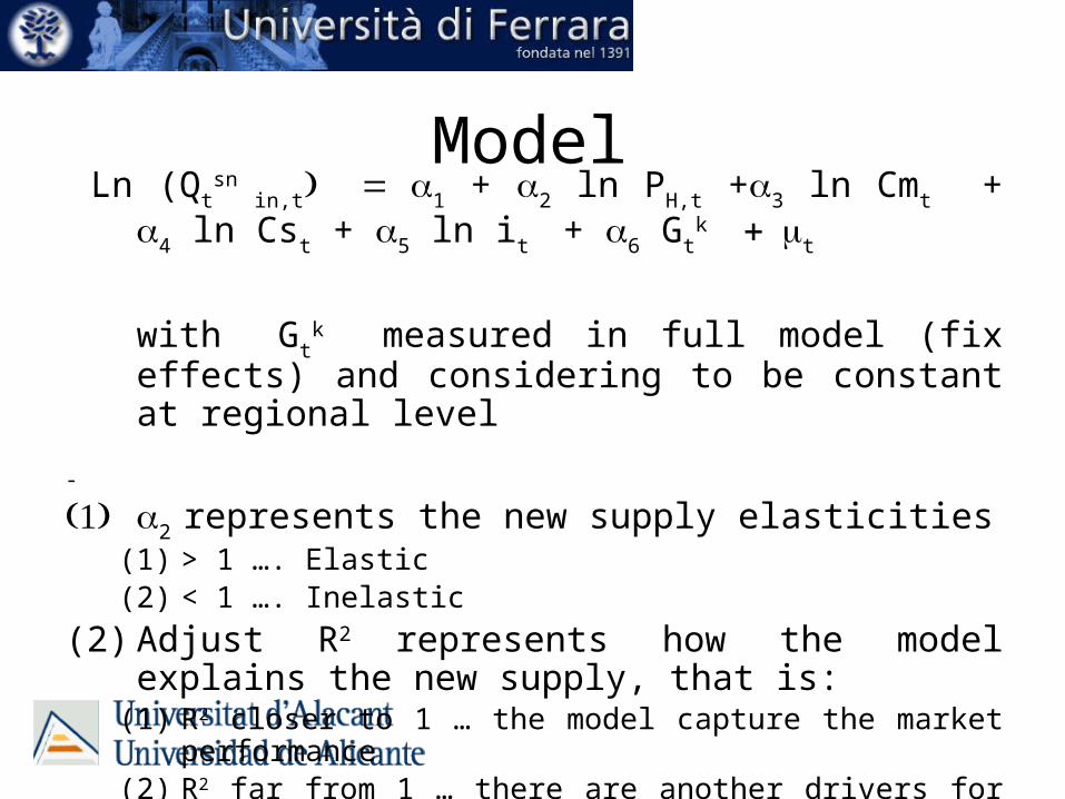
Model Ln (Qt

sn in,t) = a1 + a2 ln PH,t +a3 ln Cmt + a4 ln Cst + a5 ln it

+ a6 Gt

k + mt

with Gtk measured in full model (fix effects) and

considering to be constant at regional level

-

(1) a2 represents the new supply elasticities(1) > 1 …. Elastic(2) < 1 …. Inelastic

(2) Adjust R2 represents how the model explains the new supply, that is:

(1) R2 closer to 1 … the model capture the market performance(2) R2 far from 1 … there are another drivers for new housing supply

(construction decissions) other than the market ones.

Data• Secondary source data: National institutes of

statistics• 1995-2010 (last available)• Yearly data• By region (14 and 17)• Pool

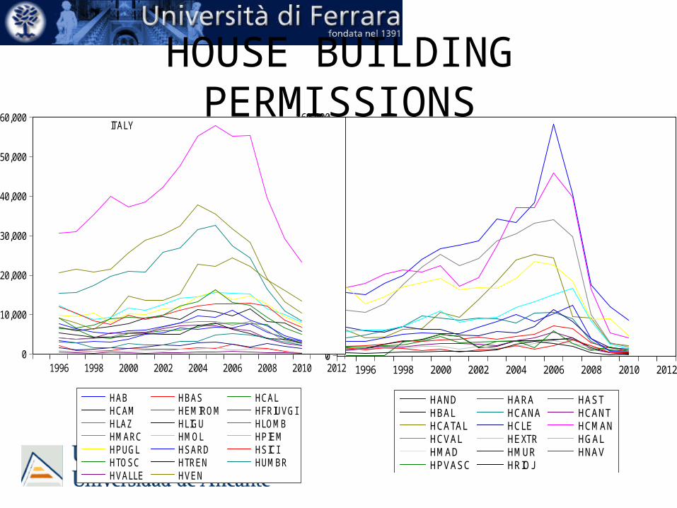
HOUSE BUILDING PERMISSIONS

0

20,000

40,000

60,000

80,000

100,000

120,000

140,000

160,000

1996 1998 2000 2002 2004 2006 2008 2010 2012

HAND HARA HASTHBAL HCANA HCANTHCATAL HCLE HCMANHCVAL HEXTR HGALHMAD HMUR HNAVHPVASC HRIOJ

0

10,000

20,000

30,000

40,000

50,000

60,000

1996 1998 2000 2002 2004 2006 2008 2010 2012

HAB HBAS HCALHCAM HEMIROM HFRIUVGIHLAZ HLIGU HLOMBHMARC HMOL HPIEMHPUGL HSARD HSICIHTOSC HTREN HUMBRHVALLE HVEN

ITALY

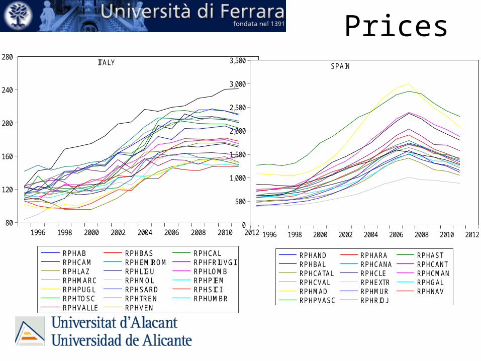
Prices

80

120

160

200

240

280

1996 1998 2000 2002 2004 2006 2008 2010 2012

RPHAB RPHBAS RPHCALRPHCAM RPHEMIROM RPHFRIUVGIRPHLAZ RPHLIGU RPHLOMBRPHMARC RPHMOL RPHPIEMRPHPUGL RPHSARD RPHSICIRPHTOSC RPHTREN RPHUMBRRPHVALLE RPHVEN

ITALY

0

500

1,000

1,500

2,000

2,500

3,000

3,500

1996 1998 2000 2002 2004 2006 2008 2010 2012

RPHAND RPHARA RPHASTRPHBAL RPHCANA RPHCANTRPHCATAL RPHCLE RPHCMANRPHCVAL RPHEXTR RPHGALRPHMAD RPHMUR RPHNAVRPHPVASC RPHRIOJ

SPAIN

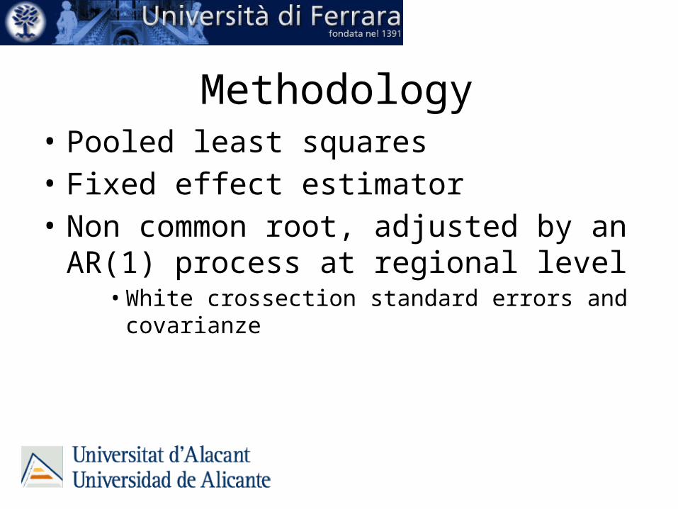
Methodology• Pooled least squares• Fixed effect estimator• Non common root, adjusted by an AR(1)

process at regional level• White crossection standard errors and covarianze

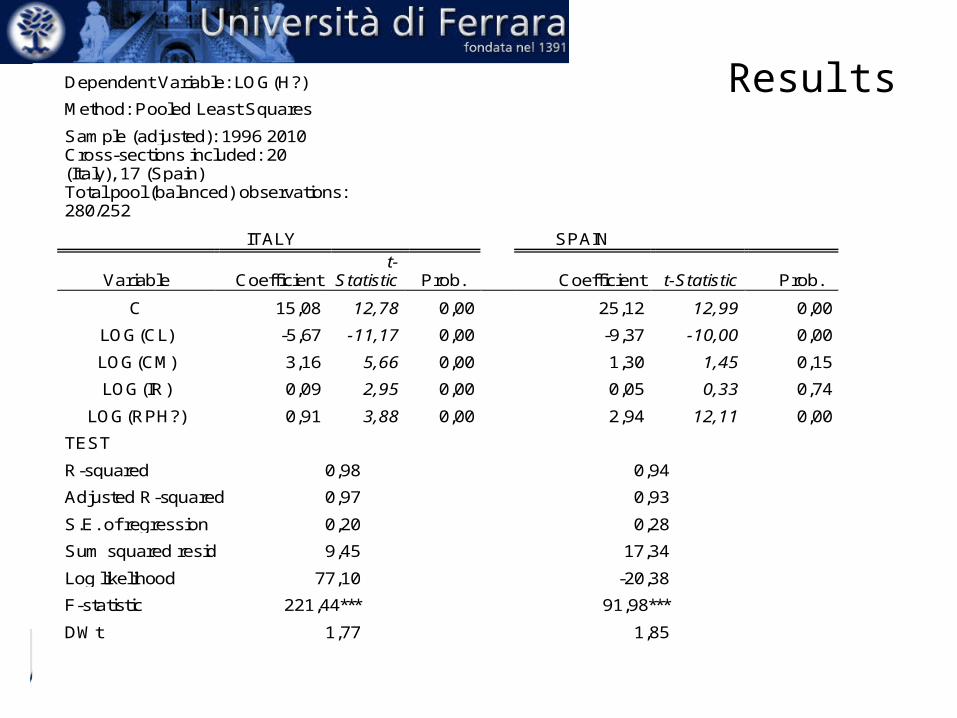
ResultsDependent Variable: LOG(H?) Method: Pooled Least Squares Sample (adjusted): 1996 2010 Cross-sections included: 20

(Italy), 17 (Spain) Total pool (balanced) observations:

280/252

ITALY

SPAIN

Variable Coefficient t-

Statistic Prob.

Coefficient t-Statistic Prob.

C 15,08 12,78 0,00

25,12 12,99 0,00

LOG(CL) -5,67 -11,17 0,00

-9,37 -10,00 0,00

LOG(CM) 3,16 5,66 0,00

1,30 1,45 0,15

LOG(IR) 0,09 2,95 0,00

0,05 0,33 0,74

LOG(RPH?) 0,91 3,88 0,00

2,94 12,11 0,00

TEST R-squared 0,98

0,94

Adjusted R-squared 0,97

0,93

S.E. of regression 0,20

0,28

Sum squared resid 9,45

17,34

Log likelihood 77,10

-20,38

F-statistic 221,44***

91,98***

DWt 1,77

1,85

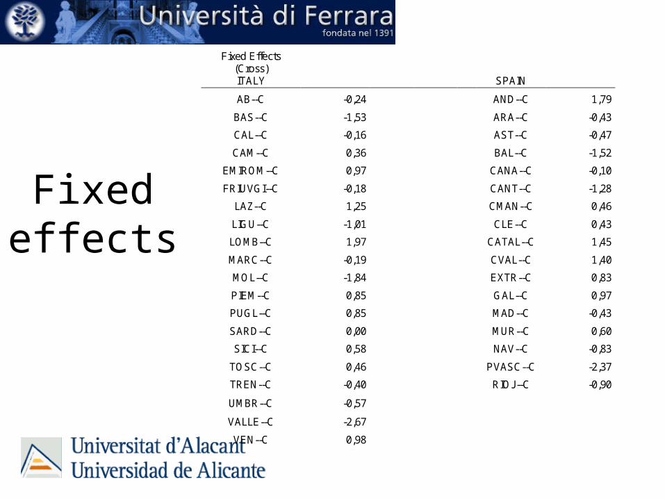
Fixed effects

Fixed Effects (Cross) ITALY

SPAIN

AB--C -0,24

AND--C 1,79

BAS--C -1,53

ARA--C -0,43

CAL--C -0,16

AST--C -0,47

CAM--C 0,36

BAL--C -1,52

EMIROM--C 0,97

CANA--C -0,10

FRIUVGI--C -0,18

CANT--C -1,28

LAZ--C 1,25

CMAN--C 0,46

LIGU--C -1,01

CLE--C 0,43

LOMB--C 1,97

CATAL--C 1,45

MARC--C -0,19

CVAL--C 1,40

MOL--C -1,84

EXTR--C 0,83

PIEM--C 0,85

GAL--C 0,97

PUGL--C 0,85

MAD--C -0,43

SARD--C 0,00

MUR--C 0,60

SICI--C 0,58

NAV--C -0,83

TOSC--C 0,46

PVASC--C -2,37

TREN--C -0,40

RIOJ--C -0,90

UMBR--C -0,57

VALLE--C -2,67 VEN--C 0,98

Conclusions (1)• Similar cycles with stronger house building in

Spain than in Italy– Higher house price growth also in Spain but during

2004-2008• Similar market reacions• Very market oriented (adjR2>0,93)

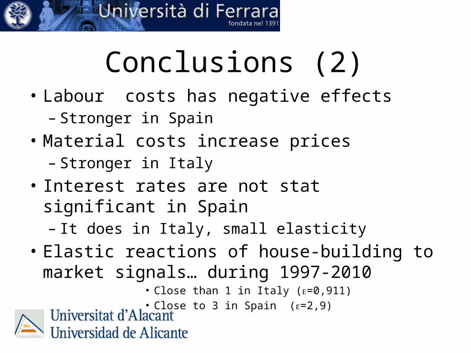
Conclusions (2)• Labour costs has negative effects

– Stronger in Spain• Material costs increase prices

– Stronger in Italy• Interest rates are not stat significant in Spain

– It does in Italy, small elasticity• Elastic reactions of house-building to market

signals… during 1997-2010• Close than 1 in Italy (e=0,911)• Close to 3 in Spain (e=2,9)

•THANKS FOR YOUR ATTENTION