Embed Size (px)
Citation preview

HOUSING WEALTH, FINANCIAL WEALTH, AND CONSUMPTION: NEW EVIDENCE FROM MICRO DATA 1
by
Raphael Bostic*, Stuart Gabriel** and Gary Painter*
January 2007 (Revised May 2008)
* Lusk Center for Real Estate, School of Policy, Planning and Development, University of Southern California, 331 Lewis Hall, Los Angeles, California 90089-0626, [email protected] (corresponding author) and [email protected] **Anderson School of Management and Ziman Center for Real Estate, University of California, Los Angeles, 110 Westwood Plaza, Suite C412, Box 951481, Los Angeles, California, 90095-1481, [email protected]. 1 The authors thank Dolores Conway, Yuming Fu, Fred Furlong, Richard Green, Don Haurin, Selo Imrohoroglu, John Krainer, Edward Leamer, Erica Morris, Albert Saiz, Mark Spiegal, Selale Tuzal and Jim Wilcox for comments on an earlier draft of this paper. We also are appreciative of feedback from the editor. We owe special thanks to Jim Kennedy of the Federal Reserve Board for discussion and inputs to the analysis. The authors also thank Jane Lincove and Abishek Mamgain for excellent research assistance.

HOUSING WEALTH, FINANCIAL WEALTH, AND CONSUMPTION: NEW EVIDENCE FROM MICRO DATA
Abstract
Fluctuations in the stock market and in house values over the course of recent years have led to renewed macroeconomic policy debate as regards the effects of financial and housing wealth in the determination of consumer spending. This research assembles a unique matched sample of household data from the Survey of Consumer Finance and the Consumer Expenditure Survey to estimate the consumption effects of financial and housing wealth. The micro-data permit numerous innovations in the assessment of wealth effects, including an analysis of the impact of wealth on both durable and non-durable consumption and a comparison of wealth effects as derive from gross versus after-debt measures of financial and housing wealth. Further, the research seeks to assess robustness of those estimates to deviations from trend and volatility in financial and housing wealth and among credit constrained and non-credit constrained households. Overall, research findings indicate relatively large housing wealth effects. Among homeowners, the housing wealth elasticities are estimated in the range of .06 over the 1989 - 2001 period. In marked contrast, the estimated elasticities of consumption spending with respect to financial wealth are smaller in magnitude and are in the range of .02. Further, the estimated wealth elasticities appear robust to deviations from trend and volatility in the wealth measures. Research findings support the hypothesized behavioral distinction in household consumption spending across durable versus non-durable categories. Consumption propensities also diverge sharply across the credit constrained and non-credit constrained households. Finally, there is little difference in wealth elasticities derived from measures of home equity versus house values. Research findings suggest the possibility of sizable reverse wealth effects. For example, a 10 percent decline in housing wealth from 2005 levels translates into a 1 percentage point decline in real GDP growth, a sizable reduction relative to the approximate 4 percent real GDP growth evidenced in recent years. Results of the analysis point to the sizable economy-wide risks associated with the recent retrenchment in house values.
2

I. Introduction
Recent years have witnessed widespread media attention and economic policy debate
regarding the consumption effects of fluctuations in household financial and housing
wealth. As is well-appreciated, stock prices evidenced pronounced volatility over the
course of the 1990s, running up by 450 percent before falling back by a full one-third
during 2000-2001. The stock market collapse destroyed more than $8 trillion in paper
wealth and was arguably a cause of the 2001 recession. In contrast, U.S. house prices
approximately doubled over the decade of the 1990s and then doubled again during 2000-
2005 in many metropolitan areas. In 2005, those gains were widespread as 25 U.S. states
recorded double-digit house price increases. Indeed, home equity grew by about $9.6
trillion during 2001-2004 to comprise more than one-half of the wealth of the typical U.S.
household [Belsky & Prakken, 2004].2 In a recent paper, Greenspan and Kennedy [2005]
estimated home equity extraction at $383 billion in 2001 and $552 billion in 2002, of
which $174 and $214 billion, respectively, consisted of gross cash out refinance activity.
According to Greenspan and Kennedy [2005], homeowners extracted an additional $300
billion in home equity through cash-out refinancings in 2003. The refinance boom of
recent years was supported by generational lows in mortgage interest rates and
innovations in financial and mortgage markets that enabled households to access their
wealth in cheaper, faster ways.3 More recently, in the wake of the 2006-2007 bursting of
2 By 2003, the value of home equity on household balance sheets exceeded the value of stocks directly owned by households by $2.6 trillion (Belsky and Prakken (2004)). According to the 1998 Survey of Consumer Finances, financial wealth is concentrated in restricted accounts. Further, 84 percent of total stock market wealth in the U.S. is held by the top income quintile. 3 See Bostic and Surette (2001) for a discussion of some of these financial and mortgage market innovations.
3

speculative bubbles both in housing and in the capital markets, house prices have
recorded substantial declines. Similar retrenchment was evidenced in mortgage re-
finance activity, in the wake of marked reductions in home equity and in related
withdrawal or re-pricing of home equity lines of credit and other mortgage products.
Those dramatic trends led analysts at the Federal Reserve and on Wall St. to ascribe a
critical role to housing wealth in the determination of cyclical swings in consumption
activity.4,5
A well developed literature in finance has established a link between consumption
and wealth shocks (e.g., Poterba and Samwick [1996], Juster et al [1999]). These models
predict that unexpected wealth shocks change the permanent income of households and
thereby affect the life-cycle pattern of savings and consumption (Lettau and Ludvigson
[2004]). A companion literature has argued that shocks to different forms of wealth can
elicit varying consumption responses (e.g., Iacoviello [2004], Lettau and Ludvigson
[2004], Piazzesi et al. [2004], Case, Shiller, and Quigley [2005], Lustig and Van
Nieuwerburgh [2005]) and empirical studies have generally borne this out (e.g., Case,
Shiller, and Quigley [2005], Benjamin, et al., [2002]).
This research assembles a unique matched data sample from the Survey of Consumer
4 In a speech to the Mortgage Bankers Association in 1999, Chairman Greenspan suggested that “One might expect that a significant portion of the unencumbered cash received by house sellers and refinancers was used to purchase goods and services…”. Greenspan further articulated the role of home equity extraction in support of U.S. economy activity in subsequent statements. 5 On January 25, 2006, Justin Lahart of the Wall St. Journal wrote “Housing is becoming a front-burner issue for Wall St. First of all, investors fret that because prices ran up by so much over the past several years, the real estate market could be in for more than a garden-variety slowdown. Second, they worry that because housing’s strength has provided a big boost to consumer spending; even a garden variety slowdown could prompt big-time belt tightening.”
4

Finance and the Consumer Expenditure Survey to estimate the consumption effects
associated with real estate and financial wealth. The highly-detailed micro data enable us
to shed new light on household consumption behavior in several important ways.
Specifically, we assess household responses among different categories of consumption
spending and to various components of financial and real estate wealth. Further, the
research evaluates variability in consumption spending to changes in the market value of
household asset holdings, as is customary in the empirical literature, and to changes in
wealth net of debt, as is consistent with theory. The analysis also examines household
responses over time and in response to volatility and trend deviations in the underlying
wealth measures, so as to assess in the robustness of the estimated elasticities to the
marked fluctuations in stock market and real estate valuations evidenced over the 1989 –
2001 period. Additional estimates are presented, including those pertaining to the
robustness of wealth estimates across households grouped by age and by credit constraint
in consumer debt markets.
The research proceeds as follows. The next section provides background and a
review of relevant literature. The dataset and empirical specifications are described in
Section III. Section IV presents the statistical results, and Section V discusses
implications of statistical findings for macroeconomic activity.
II. Background and Literature Review
Recent literature has sought to nuance our understanding of the link between
consumer behavior and shocks to household wealth. In that regard, Lettau and
Ludvigson [2004] stress that unexpected wealth shocks must be perceived as permanent
to affect consumption spending. The authors present evidence that households do not
5

respond to transitory shocks by adjusting consumption patterns.6
The literature also has posited that consumption responses can vary depending on the
type of wealth. There are several possible explanations for this. First, households may
view some forms of wealth as temporary or more uncertain (e.g., Edison and Slok [2001],
Lettau and Ludvigson [2004], Case, Shiller, Quigley [2005]). Second, households may
find it more difficult to measure or liquefy certain types of wealth. For example,
transactions costs related to borrowing against home equity could result in a lower
marginal propensity to consumer out of home equity related to stock market equity, all
things equal. Also, households with significant debts or other credit constraints may be
differentially affected by shocks to particular types of wealth. In that regard, Iacoviello
[2004] suggests that house prices should enter a correctly specified Euler equation for
consumption if household borrowing capacities are tied to the value of their houses.
Another behavioral possibility is that households “hold” different assets classes in
separate “mental accounts” (Thaler [1990]), leading them to respond differently to
changes in their gross or net positions in financial or housing wealth. For example, a
dollar made in capital gains may be considered more discretionary than a dollar in
existing wealth, especially if the capital gains in stocks or housing are largely
unanticipated and viewed as windfalls.7 Also, as suggested by Juster et al (2006), the
housing asset may serve more than one purpose—as housing is both an instrument of
6 There is not complete unanimity regarding this view, however, as some research suggests that households do not always behave in the way predicted by these standard models. Work by Choi et al (2004) suggests in a study of 401k contributions that households can respond to a positive wealth shock by saving more to take advantage of higher rates of return, and can respond to a negative shock by consuming more now. 7 As suggested by Shefrin and Thaler (1988), the marginal propensities to consume may differ across assets because of varying perceptions of liquidity. That is, for behavioral reasons, household may self-impose differing asset-based constraints on liquidity.
6

savings and a consumption good. Accordingly, while house price increases add to the
wealth of homeowners, such increases may make trade-up less affordable to households
and accordingly dampen their consumption response. Finally, a number of authors (e.g.,
Piazzesi et al. [2004], Lustig and Van Nieuwerburgh [2005]) suggest that housing may
provide consumption insurance, and therefore affect consumption patterns differently
than does financial wealth.
While not all previous work has used these theoretical justifications as their basis for
inquiry, a number of studies have investigated the possible independent roles of both
financial and housing wealth on consumption. In general, analyses of the role of housing
wealth in the determination of consumption spending have used one of three types of
information: aggregate time-series data at the state or national level, micro-data from
household-level surveys, and data based on refinance activity. The literature is
summarized in Table 1.
Elliot [1980] conducted an early study of the impact of non-financial and financial
wealth on consumption spending using aggregate data, and concluded that non-financial
wealth had no impact on consumption. In contrast, applying an error correction
framework, Belsky and Prakken [2004] find that the estimated consumption effects of
real estate and corporate equity are sizable and similar in magnitude (about 5-1/2 cents on
the dollar), but different in immediacy of impact.8 Carroll [2004] applies aggregate time-
8 The authors construct service and durable goods measures of consumption from information contained in the NIPA and the Federal Reserve’s Flow of Funds. The Flow of Funds accounts were further utilized to construct national time-series measures of housing and corporate wealth as well as to compute home equity withdrawals. Findings suggest that about 80 percent of the long-run housing wealth effect is realized within 1 year, whereas it takes close to 5 years for stock wealth to approach 80 percent of its long-run impact.
7

series data over frequencies of a few quarters to estimate housing and stock wealth
elasticities; the estimated elasticities are similar in magnitude to those of Belsky and
Prakken [2004]. However, in the Carroll [2004] study, the immediate quarterly MPC was
estimated at only 1-1/2 cents on the dollar, but accumulates gradually to about 4 - 10
cents over the ensuing couple of years. Case, Quigley, and Shiller (CQS) [2005] apply
both state- and country-level data and find that the marginal propensities to consume out
of housing wealth are substantially in excess of those for financial wealth. Dvornak and
Kohler [2003] obtain the opposite results in application of the CQS methodology to the
Australian economy, with larger effects for financial wealth, but smaller effects for
housing wealth. Benjamin, Chinloy, and Jud [2003] use U.S. state-level data similar to
that used in CSQ [2005] and find sizable housing wealth effects. Finally, Case [1992]
linked the real estate price boom in the late 1980’s in New England to a substantial
increase in consumption for the region.
A number of other studies have used the Panel Study of Income Dynamics (PSID), a
household-level survey, to investigate the relationship between housing wealth and
household consumption spending. Owing to data limitations in the PSID, these studies
evaluate only non-durable or food measures of consumption. Further, only the limited
information in the period wealth supplements of the PSID is available to measure
financial and housing wealth. Skinner [1996] finds that increases in housing wealth
result in increased consumption spending by younger households, but not by older
households, who tend to be more cautious in spending those gains.9 Engelhardt [1996]
9 Skinner (1996) also found an asymmetry in effects in that households under 45 who realized declines in housing wealth increased saving by 10 cents per dollar of decline, whereas those than realized gains decreased savings by 0.4 cents per dollar of increase.
8

identifies the marginal propensity to consume out of housing wealth to be about .03, but
finds this effect to be asymmetric and significantly associated only with declines in house
values (i.e., reverse wealth effects). Lehnert [2003] finds an overall marginal propensity
to consume of similar magnitude, but also observes variation in estimated results across
the age distribution.10 Levin [1998], using micro data from the Retirement History
Survey, finds no effect of housing wealth on consumption. In marked contrast, using
micro data from the U.K., Campbell and Cocco [2005] estimate a house price elasticity as
large as 1.7 for older households.11
In a study of mortgage re-finance activity, Canner et al. [2002] apply Survey of
Consumer Finance data to estimate the magnitudes of housing wealth extraction and
related consumption effects during 2001-2002. They find that the median household
extracted approximately $20,000 in housing equity during that period, and that 60% of
the extracted wealth went towards new consumption, whereas the remainder was used to
pay off debt. The Canner et al. [2002] analysis estimates this magnitude of home equity
extraction led to $67 billion in new consumption spending. However, the study lacks
nuanced measures of consumption and concludes that it is difficult to estimate a direct
wealth effect.
While the above studies provide important insights as regards the role of financial and
housing wealth in the determination of consumption spending, past assessments have
10 Lehnart [2003] finds the largest effects for the youngest households and for those households on the verge of retirement, who may be downsizing their housing needs. 11 Campbell and Cocco [2005] apply household data from the UK Family Expenditure Survey to estimate the response of consumption to house prices. Their model allows for regional heterogeneity in outcomes. However, owing to the pseudo-panel data structure, they are not able to precisely identify those households for whom the wealth effect of house price changes is the largest or for whom borrowing constraints are non-binding. We address those issues directly in our estimation below.
9

been constrained as regards data resources and methodology. Studies relying on
aggregate time-series data lack a clear behavioral link between fluctuations in wealth and
household spending. That is, it is not possible to identify whether increases in
consumption expenditures are incurred by those households that experienced an increase
in wealth. The macro datasets also typically lack controls for household demographic
and economic characteristics and may suffer from omitted variables and endogeneity
issues. While studies using the longitudinal PSID address concerns regarding the direct
behavioral link between consumption spending and changes in household wealth, the
PSID lacks important indices of both consumption and wealth and thus does not permit
more nuanced analyses that may be of interest to researchers and to macroeconomic
analysts. For example, studies relying on the PSID have difficulty distinguishing
between effects on durable and non-durable consumption or in evaluating responses
associated with changes in either gross or net-of-debt measures of household wealth.
Further, the PSID data lack detailed information on household asset holdings across
financial, homeownership, and other real estate classifications.
This study addresses these shortcomings directly. By combining highly-detailed
micro data on household wealth from the Survey of Consumer Finances (SCF) with
household consumption and demographic information from the Consumer Expenditure
Survey (CEX), we develop a unique micro data set that permits a careful and nuanced
investigation of the relationship between consumer spending and the various wealth
measures. In contrast to most prior research, we are able to disaggregate consumption
spending into total consumption and durable goods spending and to test for differential
wealth estimates across those categories. As suggested above, previous research largely
10

has focused on total consumption or food purchases, and the purchase of consumer
durables may be more or less affected by changes in wealth. If spending on durable
goods is predicated in part on unanticipated wealth increases or is viewed as enhancing to
diversification of the household portfolio, then durable consumption may have a greater
elasticity with respect to wealth than non-durable consumption. Alternatively, if durables
are treated as long term purchases by households, they may be less affected by short-run
fluctuations in wealth.
Another innovation is our use of household balance sheet information from the SCF
to estimate wealth effects across financial, housing and other forms of wealth.
Information in the SCF on household wealth is sufficiently detailed so as to permit the
separation of holdings of owner-occupied real estate from other forms of real estate and
to estimate related wealth effects. While very few households hold other forms of real
estate, asset values in these markets are more volatile than those of owner-occupied
housing, and therefore may have a different impact on consumer spending.
Further, we test whether households base their consumption decisions on the market
value of their asset holdings or on those wealth measures net of debt. To our knowledge,
only one prior study of consumption spending (Dvornak and Kohler [2003]) has used a
measure of net wealth – in this case, home equity – to assess housing wealth effects.
That analysis, however, was confined to aggregate data. Other relevant studies examine
the relationship between consumption and asset market values. The estimated
relationship is then taken to represent wealth effects. However, this equivalence need not
hold. For example, households may less accurately assess their net asset position,
introducing measurement error that could bias the estimated net wealth coefficients
11

downwards.
Also, we establish whether wealth shocks have induced variability in household
consumption responses over time. To do so, we estimate the financial wealth and
housing wealth elasticities cross-sectionally for the 1989, 1992, 1995, 1998 and 2001
survey years. We then pool data from the 1989 – 2001 survey years so as to evaluate the
robustness of the estimated financial and housing wealth elasticities to deviation from
trend and volatility in the household financial and housing wealth measures. Such an
analysis, not previously done, helps to shed light on the stability of household behavioral
responses to wealth shocks and also provides insights as to the importance of housing
cycle and other economic considerations for household consumption decisions. Finally,
we investigate the robustness of estimation results across the age distribution and among
household with impaired borrowing capacity, with the latter test providing an evaluation
of the Iacoviello [2004] Euler equation hypothesis.
III. Data and Model
As noted above, our research relies on a dataset that was expressly developed so as to
allow appropriately nuanced specification of the wealth-related hypotheses. That dataset
links detailed individual-level consumption information with similar quality wealth data
and accordingly is substantially better suited to the questions at hand than the data used in
prior studies. The data are drawn from two surveys. The U.S. Bureau of Labor
Statistics’ Consumer Expenditure Survey (CEX) has since 1980 collected detailed
information about U.S. household expenditures.12 Detailed indicators of household
12 The CEX consists of two surveys. In the Diary survey, respondents track expenses on frequently purchased items such as food over a two-week period. In the Interview survey, which is conducted quarterly, respondents report on regular expenses, such as
12

financial and housing wealth are drawn from the Federal Reserve Board’s Survey of
Consumer Finances.
We use information obtained from the CEX to calculate a household’s consumption-
related expenses for a calendar year. For our purposes, we track total expenses, as well
as expenses on durable goods. Our CEX sample also includes demographic information
on the households, such as the age, race, marital status, housing tenure, and level of
education of the household head. Unfortunately, the wealth data in the CEX is limited in
terms of scope and precision, and thus the CEX alone is not sufficient for our purposes.13
We therefore turn to a different survey that specializes in household wealth and
income, the Federal Reserve Board’s Survey of Consumer Finances (SCF). The SCF is a
triennial survey of U.S. households that provides highly detailed information on U.S.
families’ assets and liabilities, use of financial services, income, and housing and
demographic characteristics. Importantly, the SCF oversamples relatively wealthy
households to ensure strong coverage of households with significant financial holdings.14
This survey provides far more information about a household’s balance sheet and
financial position than any other survey of households. It thus is an ideal instrument to
address our question of how consumption varies with the market value of a household’s
assets as well as with the net wealth position of those households.
The particular variables of interest are the asset value and net wealth measures. Our
analysis includes each household’s financial assets, the value of the household’s home if
monthly bills, and major expenses of large items. 13 See Dynan and Maki (2001). 14 The SCF is sponsored by the Board of Governors of the Federal Reserve System in cooperation with the U.S. Department of the Treasury, and conducted by the Survey Research Center at the University of Michigan. For more on the sampling technique used in the SCF, see Kennickell (2000).
13
they own it, and the value of any other real estate the household might own.15 We also
use SCF information on consumer debt and mortgage debt associated with both owner-
occupied and the other real estate in the household’s portfolio to compute the household’s
net wealth position. The SCF data also include demographic variables such as age, race,
marital status, years of education, and housing tenure status that are important for the
matching procedure.
Although both the CEX and SCF began in the early 1980s, because the SCF question
frame changed prior to the 1989 survey, comparisons across years are only appropriate
for surveys implemented from 1989 to the present. The analysis therefore examines the
1989 to 2001 time period, and uses responses associated with the 1989, 1992, 1995,
1998, and 2001 SCF and CEX surveys. The study further includes information from the
Wilshire 5000 Index and the regional repeat sales house price indices of the Office of
Federal Housing Enterprise and Oversight (OFHEO) on performance of stock and
housing markets over the 1989 – 2001 study period. The latter indices are utilized to
assess the robustness of the estimated financial and housing wealth elasticities to
deviations from trend and volatility in housing and stock prices. To create an ideal
dataset, we match observations across the SCF and CEX, a process that is described in
the following section.
The Matching Procedure
Because the CEX and SCF do not survey the same households, linking the
consumption data in the CEX with the detailed wealth data in the SCF requires a
15 Financial assets in the SCF are calculated as the sum of liquid assets, certificates of deposit, mutual funds, stocks, bonds, other managed assets, cash life insurance, and quasi-liquid retirement savings.
14

matching algorithm. We use a nonparametric procedure suggested by Goel and
Ramalingam [1989] that first partitions both samples into cells based on individual
characteristics known to be highly-correlated with variation in consumption, such as age,
marital status, and education. As a precaution, the dimensionality of these characteristics
was restricted to increase the likelihood that cells were not empty for either sample. For
this paper, the match was established along four dimensions:
Marital status – Married or not;
Race – white, black, or other;
Level of schooling – Less than high school, high school graduate, some college,
college degree or more; and
Age – 25-35, 36-50, and 51-65;
Based on the matching dimensions, we partitioned the sample into 72 cells, within which
the CEX and SCF observations were matched. Given the focus of the analysis and to
mitigate against matching across tenure status, the sample was restricted to homeowners.
The sample was further restricted to household heads between 25 and 65 years of age to
eliminate issues regarding heterogeneous consumption during college-age years and
retirement. The match process yielded a dataset with 2759 observations in 2001.
Matching within a cell proceeded as follows. CEX observations were rank ordered
by income. SCF observations were likewise ranked by income, with each SCF
observation included four times to ensure that each CEX observation had a match. From
this “quadrupled” SCF sample, a random sample was drawn of a size equal to the number
of CEX observations. The two sets of rank ordered samples – the CEX sample and the
15

randomly-drawn SCF sample – were then matched one-to-one.16 Given the over
sampling of high income households in the SCF, we truncated that sample in each year at
90 percent of observed household income, so as to enhance to comparability of the SCF
and CEX income matches.17,18
Each observation in the matched sample includes a measure of income from both the
SCF and CEX. As a check of the match procedure, we compared the correlations
between the two measures of income and between the income measures and the
consumption and wealth variables that appear exclusively in only one or the other of the
surveys. Those correlations are displayed in Table 2 for the 2001 survey year.19 Note
that the two income measures are highly correlated. Further, the correlations between the
SCF income variable and the CEX consumption variables are stronger than the within
CEX correlations, and their rank orderings and relative magnitudes remain intact across
the surveys, which offers a degree of confidence in the quality of the match. This
relationship is also observed regarding the SCF wealth variables, where the CEX income
correlations are similar in magnitude to those of the SCF.20
16 That is, the CEX observation with the highest income was matched to the SCF observation with the highest income, the second highest CEX income to the second highest SCF income, and so on. 17 In most cases, this type of matching procedure will be comparable to other more sophisticated statistical matching techniques. For more, see Goel and Ramalingam (1989). 18 The estimated results were robust to the income truncation algorithm. 19 Correlation coefficients are computed for the other survey years and are of similar magnitude to those displayed in Table 2. They are available from the authors upon request. 20 As a further check of our method, the matching procedure was reapplied to a sample in which the SCF observations were not ranked by income. The correlation between CEX income and SCF income fell dramatically from over .8 to about .2, providing some evidence suggesting that the sampling and matching process employed is not introducing undue biases.
16

The nonparametric procedure described above is also known as statistical matching
(Singh et al. [1993]). The challenge in implementing such a procedure is that the
resulting dataset will violate the conditional independence assumption (Barry [1988])
across matched datasets. We overcome this in two ways. First, as described, we
implement a constrained matching procedure, which is much less likely to suffer from
this deficiency (Rodgers [1984]). Further, we implement a bootstrap procedure to guard
against the possibility that an idiosyncratic match might drive the results, and to obtain a
measure of confidence regarding the robustness of parameter estimates. All regressions
(described below) were estimated 100 times, each associated with a different draw from
the matching procedure. The parameters reported in the results section represent the
average parameter values and the standard error of the parameter estimates over the 100
runs.
The Empirical Specification
The standard approach in the literature has been to establish a relationship between
the market value of assets and consumption, controlling for income. As summarized
above, these approaches have included both time series and simple cross sectional
models. Regardless of approach, none of the prior papers have made any claim as to the
causal impacts of the wealth effects, as it is difficult to imagine an instrument that would
be predictive of wealth, yet unrelated to unobserved factors that affect consumption.
While this paper similarly is unable to propose an uncontaminated instrument, we are
able to further refine the estimates of wealth effects by utilizing better data than past
analyses and by conducting a large number of robustness checks across various sub-
samples. These latter results using stratified samples seek to address concerns about
17

unobserved variables and provide confidence that the results are not unduly influenced by
a particular subset of the population or by a particular definition of consumer spending.
Our basic empirical model is a reduced form and is estimated at the household-level;
a logarithmic transformation is required to linearize consumption, income, and wealth,
and so the standard specification is:
(1) log C = f (log Y, log V, Z),
where C is consumption, Y is current income, V is asset value, and Z is a vector of
household demographic, human capital and like controls.21
Our approach expands the standard methodology in two ways. First, it disaggregates
asset value and evaluates the relationship between consumption and the various
components of asset value. In the context of the standard methodology, this modifies
equation (1), but only slightly, as the components of asset value also need to be linearized
using the log transformation:
(2) log C = f (log Y, log Vf, log Vh, log Vr, Z),
where Vf is the value of the individual’s financial holdings, Vh is the value of the
individual’s primary residence, and Vr is the value of the other real estate assets an
individual holds.
The second innovation – the introduction of debt considerations – complicates matters
21 Together, the components of Y, V, and Z serve to proxy household permanent income. In fact, Goodman and Kawai [1982] compute household permanent income by regressing Y on V and Z. Our specification is common to the literature that seeks to cull out the separable effects of household wealth and socio-demographic characteristics on consumption propensities. Note further that those households in the upper and lower tails of the income distribution are most likely to experience transitory shocks to current income. Accordingly, we tested the sensitivity of our results to exclusion from the sample of the top ten percentile and bottom ten percentile of the income distribution. Results are available from the authors upon request; they suggest that the estimated consumption elasticities are robust to the various sampling algorithms.
18

a bit more. The existence of negative values, which can arise if debts exceed asset value,
means that our more comprehensive characterization of an individual’s overall financial
position can not be transformed using the log function. Fortunately, the difference of two
log-normal variables is normal. Thus, if debts are distributed comparably to asset values,
the difference between the asset values and debt is normally distributed and can be
estimated untransformed in a standard regression framework. For this portion of the
analysis, we therefore estimate
(3) log C = f (log Y, Vf – D, Vh – M, Vr – Mr, Z)
where D represents non-real estate debt, M is the value of the mortgage on the
individual’s primary residence, and Mr is the total value of mortgages associated with the
other real estate assets held by the individual.
In the empirical analysis to follow, equations (2) and (3) are estimated cross-
sectionally using micro data from the 1989, 1992, 1995, 1998, and 2001 survey periods.
Those equations allow for estimation and assessment of drift in the estimated wealth
elasticities over the study period. We also estimate the above models by pooling data
over the survey years. The pooled models enable the introduction of interactive terms to
explicitly assess the robustness of the estimated wealth elasticities to deviations from
trend and volatility in measures of stock market and housing wealth. The pooled models
further include year-specific fixed effects. The pooled models are specified as follows:
(4) C = f (log Y, log Vf, log Vh, log Vr, log Vf*devWil5000, logVf*volWil5000,
log Vh*devOFHEO, log Vh*volOFHEO, year fixed effects, Z),
where the year-specific household financial and housing wealth terms are interacted
with deviations from trend and computed volatility over the prior three years in the
19

Wilshire 5000 and the regional OFHEO repeat sales quality-adjusted house price indexes,
respectively.22 To the extent that households view the computed drift and volatility in
household financial and housing wealth as transitory, one would anticipate little
significant effect of those terms on consumption spending. As suggested above, we also
stratify equations (2) – (4) above across total consumption and durable goods
consumption. If spending on durable goods is predicated in part on unanticipated
changes in wealth or is viewed as enhancing the diversification of the household
portfolio, then it is possible that durable consumption may have a greater elasticity with
respect to wealth than non-durable consumption. Alternatively, if durables are treated as
long term purchases by households, they may be less affected by short-run fluctuations in
wealth.
IV. Results
The estimated income, financial wealth, and housing elasticities as derive from the
cross-sectional models (equation 2) are displayed in Table 3. As suggested above, that
specification estimates consumption elasticities associated with the market value of real
estate and financial assets. Table 4 specifies the estimating equations in terms of net
wealth measures (e.g., asset values net of mortgage or other debt as described in equation
3, above). The estimates are computed for each of the 1989, 1992, 1995, 1998, and 2001
SCF survey years, so as to facilitate assessment of variability in consumption wealth
elasticities over a period of substantial volatility and structural change in U.S. financial
and housing finance markets. For the sake of parsimony, the tables display only the
22 The pooled models are estimated for the gross wealth specifications alone, owing to limitations in data pertaining to changes over time in household debt required for computation of deviations from trend and volatility in measures of household net wealth.
20

estimated elasticities for the income, financial wealth, housing wealth and other real
estate wealth terms. Also, each of the tables displays the estimated elasticities for total
and durable goods consumption.23 Finally, table 5 displays results of estimation of
models which pool observations over the 1989 – 2001 survey years (equation 4). As
suggested above, those models also include controls for year-specific fixed effects and
for deviation from trend and volatility in financial and housing asset values. While the
primary coefficients of interest are displayed in tables 3 through 5, full regression results
are contained in appendix tables B through F. 24 Variable definitions are contained in
Appendix A.
In both year-specific and pooled models, our results generally conform to those of the
earlier literature in that both household income and financial and housing wealth are
shown to exert significant positive effects on total consumption.25 Moreover, the
sensitivity of total consumption to an asset’s value is larger for housing than for financial
holdings. As evidenced in table 3, the estimated house value elasticities range from .044
in 1998 to .065 in 2001 and are highly significant throughout. In marked contrast, the
estimated elasticities of consumption spending with respect to financial wealth are
smaller in magnitude and trend down modestly from .023 in 1992 to .018 in 1998; in
2001, the financial wealth elasticity of .007 is not precisely estimated. Overall,
23 Results for nondurable consumption are available from the authors upon request. 24 Among control variables, in the year-specific analyses we observe a monotonic relationship between the level of education and consumption for both total and durable goods consumption. In addition, consumption propensities are sizable and significant for married and separated households and for larger families. Relative to the Midwest, consumption propensities also appear to be elevated in the Northeast and West. 25 In a parsimonious specification which excludes the household socio-demographic controls, the estimated durable consumption elasticity with respect to income ranges from about .64 in 1989 to .42 in 2001. As evidenced in Table 3 and in related appendix tables, the inclusion of the socio-demographic controls serves to mediate those effects.
21

estimation findings suggest a modest decline in the importance of financial wealth to
consumption spending over the course of the 1990s.
Research findings further indicate some variability in consumer behavior across the
durable and total consumption spending. During the 1990s, housing asset value
elasticities associated with durable goods consumption--at about 0.04--are of somewhat
diminished magnitude and statistical significance relative to the elasticities for total
consumption.26 By contrast, for most years, the elasticity of durable goods consumption
with respect to changes in financial assets was estimated to be modestly larger than that
associated with total consumption.27
Table 4 further presents our estimates of equation 3, in which we introduce debt and
characterize a household’s position in terms of net wealth. The value of each of the asset
classes is computed net of debt; for example, house value is replaced by home equity and
the value of other real estate is similarly defined as other real estate equity. Results here
indicate a less precise relationship between home equity and total consumption, perhaps
owing to the fact that some households spend out of passive savings, whereas others
finance their consumption via the acquisition of debt.28 The estimated coefficients do
trend down over the period of the analysis. Given the mean home equity value of
26 In contrast, house value fluctuations appear to be more important to non-durable goods consumption. In the cross-sectional analyses, the estimated elasticities (not shown) were close to .06, highly significant, and relatively stable across estimation years. Those results are available from the authors upon request. 27 Consumption of durable goods is more sensitive to changes in household income than is total consumption. 28 Juster et al (2006) estimate the effect of capital gains on saving by asset type. In so doing, they distinguish among active and passive savings and across housing and other asset classes. Results of their analysis suggests that over five-year periods, the effect of capital gains (passive savings) in corporate equities on saving is substantially larger than the effect of capital gains on housing or other assets.
22
$176,000 in 2001 for the truncated SCF sample, the elasticity of consumption spending
with respect to home equity was computed to be about .02 in 2001, down from
approximately .04 in 1989.29 Results suggest the possibility of household measurement
error in assessing net wealth positions, whereby consumption decisions are more
sensitive to the more readily known nominal (gross-of-debt) market value of housing than
to net housing equity holdings.30
In the pooled sample (table 5), the estimated elasticities of consumption with respect
to house values and financial wealth are about .06. and .02, respectively. Results further
indicate significant negative coefficients associated with the interactions of house value
with deviations from trend and volatility in the house price term.31 Those results are
consistent with the theoretical notion (Lettau and Ludvigson [2004], Case, Shiller and
Quigley [2005]) that deviations from trend or volatility in house values, if viewed by
households as transitory in nature, may not be factored into permanent income nor
reflected in elevated consumption.32 Pooled estimation results further indicate a
statistically significant but economically modest impact of non-owner occupied housing
real estate holdings on consumer spending. The pooled results also indicate the
sensitivity of consumer spending to the stage in the economic cycle, as evidenced by the
highly significant estimates of the year-specific fixed effects.
29 Here we convert the estimated coefficients of the semi-log net wealth specifications into elasticities. The non-truncated mean home equity value of $301,914 for 2001 yields an estimated elasticity of .03 for that year. 30 These results are also consistent with a behavioral theory of differential household sensitivity to alternative wealth categories (Thaler [1990]). 31 Those terms are computed based on historical values of the OFHEO regional house price series over the previous three years. 32 In contrast, the log deviations from trend in financial wealth interactive term enters the equation with a positive and significant coefficient, suggesting that consumers attach more permanence to that measure of financial wealth.
23

V. Supplemental Findings
In supplemental analyses, we also investigated the effects on household spending
of (a) quantity constraints on credit extensions and (b) borrower credit quality. As
regards the former, the theoretical literature suggests that household borrowing capacity,
which can be influenced both by a household’s credit rating and level of outstanding
debt, should play a role in shaping how changes in different forms of wealth affect
consumption (Iacoviello [2004]; Piazzesi et al [2004]). If borrowing capacity (Iacoviello
[2004]) affects the ability of households to consume out of increases in asset values, then
we would expect households with high LTV's to be more sensitive to a relaxing of the
constraint on of their borrowing capacity. To evaluate this possibility, we included two
additional variables in equation (2): a categorical variable which is equal to one if a
household has an LTV over 90% and an interaction term of this categorical variable and
the house price variable. Despite evidence in Iacoviello [2004] that these issues are
important, both variables proved insignificant in our models.
Regarding borrower credit quality, households were grouped according to whether or
not they were credit-constrained based on a definition of such from the SCF that has been
used in previous research (Gabriel and Rosenthal [2005]).33 Given these definitions,
model (2) was re-run limiting the sample to either credit constrained or non-credit
constrained households (Table 6). Contrary to expectations, the estimated findings are
not significantly different among households who are credit constrained. One may have
expected credit constrained households to have more sensitivity to income and wealth,
33 Specifically, households are coded as credit constrained if they responded in the survey that they were turned down for a loan, partially turned down for a loan, or failed to apply for a loan owing to fears that the application would be rejected.
24

but the pattern of coefficients over time does not reveal any systematic differences.
Further, due to smaller sample size, the financial wealth and housing value coefficients
often fail to achieve accepted levels of statistical significance in the credit constrained
sample.
Finally, akin to Skinner [1996] and Lehnart [2003], we investigated the robustness of
estimation results across the age strata (not shown). Like those studies, we find
significant variability in estimated income and wealth elasticities among age cohorts.
However, our research shows both damped wealth elasticities and elevated income
elasticities among households aged 25-35, relative to older age cohorts. As anticipated
by the lifecycle hypothesis, income elasticities are found to decline whereas wealth
elasticities increase during the peak earnings years. These results stand in contrast to
those of Skinner [1996] and Lehnart [1996], who estimated elevated wealth elasticities
among younger households.34
VI. Conclusion
This research assembled a unique matched data set from individual files of the Survey
of Consumer Finances and the Consumer Expenditure Survey to estimate the
consumption effects associated with housing and financial wealth. Estimates are
provided for all survey years of the Survey of Consumer Finances from 1989 – 2001, so
as to assess any significant drift in estimated elasticities as might derive from the larger
business cycle, evolution in mortgage finance and the like. Further, year-specific data
from those survey years is pooled so as to test the robustness of the estimated wealth
34 Full estimation results for the regressions using the constrained and non-constrained samples, as well as all regression results for the samples partitioned by age are available from the authors upon request.
25

elasticities to deviations from trend and volatility in household financial and housing
asset values.
Overall, research findings indicate relatively large housing wealth effects. Among
homeowners, the house value elasticities are estimated in the range of .06 over the course
of the 1989 – 2001 study period and are highly significant throughout. In marked
contrast, the estimated elasticities of consumption spending with respect to financial
wealth, while largely significant, are smaller in magnitude and are in the range of .02.
Results from a sample of data pooled over the 1989 – 2001 study period indicate that the
estimated financial and housing wealth elasticity estimates are sensitive to controls for
deviation from trend and volatility in household financial and housing wealth. Finally,
we conducted numerous robustness tests across various sub-samples of the data that
confirm the main findings of the analysis.
The sizable consumption elasticity estimated for housing wealth, together with the
marked run-up in housing wealth over the course of recent years, point to the sustaining
influence of housing wealth on the U.S. economy during a period of financial market
weakness. Data from the Fed’s Flow of Funds accounts indicate that household financial
and real estate wealth accounted for 1-1/2 and 12-1/4 percent, respectively, of the growth
in personal consumption expenditures over the 2001:Q1 – 2005:Q3 period.35 Those same
35 Data from the Federal Reserve Board’s Flow of Funds accounts indicate that household financial wealth trended down from $33 billion in 2000:Q4 to about $29 trillion in 2003:Q1 before rebounding to $38 trillion in 2005:Q3. In marked contrast, the value of real estate owned by households recorded appreciable gains throughout the entirety of the recent period, from about $11.4 billion in 2000:Q4 to $19.1 billion in 2005:Q3. Given average values of financial and real estate assets owned by households of $32.6 and $14.9 billion, respectively, over the 2001:Q1 – 2005:Q3 period, the estimated financial and housing wealth elasticities of 0.02 and 0.06, respectively imply that financial and real estate wealth accounted for 1-1/2 and 12-1/4 percent of growth in personal consumption
26

household finance and real estate wealth effects comprised about 1 and 9 percent of U.S.
GDP growth over that same period.
Those same computations suggest the possibility of sizable reverse wealth effects in
the context of a retrenchment in house values. For example, a “back of the envelope”
partial equilibrium computation, based on the above estimation findings, suggests that a
10 percent decline in housing wealth from 2005 levels (equivalent to a roll back in wealth
holdings to about 2004 levels), would result in a $105 billion or 1.2 percent contraction in
personal consumption expenditures. Given the level of real GDP in 2005, the housing-
related decline in PCE would be roughly equivalent to a 1 percentage point reduction in
real GDP growth, a sizable reduction from the approximate 4 percent real GDP growth
estimated for recent years.
expenditures, respectively, over that period.
27

References
Barry J. T. (1988), “An Investigation of Statistical Matching”, Journal of Applied Statistics, 1988, 15, pp. 275-283.
Belsky, Eric, and Joel Prakken (2004), “Housing Wealth Effects: Housing’s Impact on
Wealth Accumulation, Wealth Distribution and Consumer Spending.” National Center for Real Estate Research Report W04-13. Boston: Harvard University. http://www.jchs.harvard.edu/publications/finance/w04-13.pdf
Benjamin, John D., Peter Chinloy and G. Donald Jud (2004), “Real Estate Versus
Financial Wealth in Consumption.” Journal of Real Estate Finance and Economics 29 (3), 341-354.
Bhatia, Kul B. (1987). “Real Estate Assets and Consumer Spending”, Quarterly Journal
of Economics, 102, 437–44. Bostic, R. W. and B. J. Surette (2001), “Have the Doors Opened Wider? Trends in
Family Homeownership Rates by Race and Income,” Journal of Real Estate Finance and Economics 23 (November), 411-434.
Karl E. Case, John M. Quigley, and Robert J. Shiller (2005) "Comparing Wealth Effects:
The Stock Market versus the Housing Market", Advances in Macroeconomics: Vol. 5: No. 1, Article 1. http://www.bepress.com/bejm/advances/vol5/iss1/art1.
Campbell, J. and Cocco, J. (2005) “How Do House Prices Affect Consumption?
Evidence from Micro Data”, NBER Working Paper 11534, August 2005. Carroll, C. (2004) “Housing Wealth and Consumption Expenditure”, Paper prepared for
the Academic Consultants meeting of the Board of Governors of the Federal Reserve System, January 2004.
Canner, Glenn, Karen Dynan, and Wayne Passmore (2002), “Mortgage Refinancing in
2001 and early 2002,” Federal Reserve Bulletin, December, 469-481. Choi, James J., David Laibson, & Brigitte C. Madrian, and Andrew Metrick (2004).
“Consumption-Wealth Comovement of the Wrong Sign,” NBER Working Paper 10454.
Dynan, K. and D. Maki (2001), “Does the Stock Market Wealth Matter for
Consumption?”, Working Paper, Division of Research and Statistics, Board of Governors of the Federal Reserve System, Washington, D.C, 2001-23.
Edison, H. and T. Slok (2001), “Wealth Effects and the New Economy”, Working Paper,
International Monetary Fund.
28

Engelhardt, Gary V. (1996), “House Prices and Home Owner Saving Behavior,” Regional Science and Urban Economics, 26(3/4), 313-336.
Gabriel, S. and S. Rosenthal (2005) “Homeownership in the 1980s and 1990s: Aggregate
Trends and Racial Disparities”, Forthcoming in the Journal of Urban Economics. Goel, Prem K. and T. Ramalingam. 1989. The Matching Methodology: Some Statistical
Properties, Lecture Notes in Statistics Series, J. Berger, et al. (Eds.), Number 52, Springer-Verlag: New York.
Goodman, A. C. and M. Kawai (1982), Permanent Income, Hedonic Prices and Demand
for Housing: New Evidence, Journal of Urban Economics, 12, 214-37. Greenspan, Alan and James Kennedy (2005), “Estimates of Home Mortgage
Originations, Repayments, and Debt on One-to-Four-Family Residences”, Finance and Economics Discussion Series 2005-41, Board of Governors of the Federal Reserve System, Washington, D.C.
Dvornak N and M Kohler (2003). “Housing Wealth, Stock Market Wealth and
Consumption: A Panel Analysis for Australia” Reserve Bank of Australia Research Discussion Paper, RDP2003-07.
Iacoviello, Matteo (2004), “Consumption, House Prices and Collateral Constraints: a
Structural Econometric Analysis,” Journal of Housing Economics, 13(4), 305-321. Juster, Thomas, James P. Smith, and Frank Stafford (1999). “The Measurement and
Structure of Household Wealth.” Labor Economics, 6, 253-275. Juster, Thomas, Joseph Lupton, James Smith, and Frank Stafford (2006) “The Decline in
Household Saving and the Wealth Effect,” The Review of Economics and Statistics, 88(1), 20-27
Lehnart, Andreas (2002), “Housing Consumption and Credit Constraints”, Federal
Reserve Board working paper. Martin Lettau and Sydney C. Ludvigson (2004). “Understanding Trend and Cycle in
Asset Values: Reevaluating the Wealth Effect on Consumption,” American Economic Review, 94(1), 276-299.
Laurence Levin (1998). “Are Assets Fungible?: Testing the Behavioral Theory of Life-
Cycle Savings,”Journal of Economic Behavior & Organization, 36(1), 59-83. Lustig, Hanno and Stijn Van Nieuwerburgh (2005). “Housing Collateral, Consumption
Insurance and Risk Premia: an Empirical Perspective,” Journal of Finance, Vol. 60 (3), pp.1167-1219.
29

Poterba, James M. and Samwick, Andrew A (1996). “Stock Ownership Patterns, Stock Market Fluctuations, and Consumption.” NBER Working Paper No. 2027
Piazzesi, Monika, Martin Schneider, and Selale Tuzel (2004). “Housing, Consumption,
and Asset Pricing,” working paper, Graduate School of Business, University of Chicago.
Rodgers W. L. (1984), “An Evaluation of Statistical Matching”, Journal of Business and
Economic Statistics, 2, pp. 91-102. Shefrin, Hersh M. and Richard Thaler (1988), “The Behavioral Lifecycle Hypothesis,”
Economic Inquiry, 26 (4), pp. 169-177. Singh A. C., Mantel H., Kinack M. and Rowe G. (1993), “Statistical Matching: Use of
Auxiliary Information as an Alternative to the Conditional Independence Assumption”, Survey Methodology, 19, pp. 59-79.
Skinner, Jonathan S. (1996), “Is Housing Wealth a Sideshow? In Advances in the
Economics of Aging, National Bureau of Economic Research Report, pp. 241-268. Chicago, Il: University of Chicago Press.
Thaler, Richard (1990): “Anomalies: Saving, Fungability, and Mental Accounts,”
Journal of Economic Perspectives, 4, 193-206
30

31
Table 1. Selected studies on wealth effects on consumption Data Measure of
housing/financial wealth
Housing wealth effect
Financial wealth effect
Studies using aggregate data
Case, Quigley, and Shiller (2005)
Panel of countries and panel of U.S. states
Aggregate housing and financial wealth
.11-.17 (Int’l),
.05-.09 (States) 0 (Int’l), .02 (States)
Benjamin, Chinloy, and Jud (2002)
U.S. national time series of states
Aggregate housing and financial wealth net of debt outstanding
.08 .02
Dvornak and Kohler (2003)
Panel of Australian states
Aggregate housing and financial wealth net of debt outstanding
.03 .06-.09
Bhatia (1987) U.S. Census, National accounts
Self-reported home values, no financial
.32-.53 ---
Studies using household surveys
Lehnert (2003) Panel Survey of Income Dynamics (PSID)
Self-reported home values, no financial
.04-.05, varies with age
---
Engelhardt (1996) PSID Self-reported home values less improvement value, no financial
.14, .03 for median household
---
Skinner (1996) PSID Self-reported home values, no financial
---
Levin (1998) Retirement History Survey
Housing equity (net of debt), financial wealth
.06, .05 for liquidity constrained
Less than .02
Studies using refinance activity
Canner, Dynan, and Passmore (2002)
Survey of U.S. households
Cash extracted via mortgage refinancing, no financial
.60 of refinance dollars
---
NOTE: Wealth effects reflect increase in consumption spending associated with a 1 unit increase in wealth or net wealth.

Table 2. Comparison of correlation coefficients for variables across the surveys
CEX SCF
log (income) log (income) CEX log(income) 1.000 0.759*** SCF log(income) 0.759*** 1.000
CEX consumption variables Total 0.406*** 0.434*** Nondurable 0.202*** 0.202*** Durable 0.452*** 0.496*** Food 0.283*** 0.330***
SCF wealth variables Financial 0.146*** 0.153*** House value 0.296*** 0.366*** Other real estate 0.094*** 0.123*** Net financial 0.141*** 0.146*** Correlation results are from one matched sample from 2001 CEX and SCF *** p< .001
32

Table 3. Homeowners: Market value regression results 1989 1992 1995 1998 2001 Total Consumption
log(income) 0.162*** 0.198*** 0.188*** 0.197*** 0.191***
(0.012) (0.013) (0.012) (0.015) (0.012)
log(financial wealth) 0.021*** 0.024*** 0.023*** 0.018** 0.020***
(0.005) (0.005) (0.005) (0.006) (0.005)
log(house value) 0.060*** 0.050*** 0.050*** 0.046** 0.042***
(0.011) (0.013) (0.014) (0.016) (0.012)
log(other real estate) 0.008*** 0.006** 0.006** 0.004 0.005*
(0.002) (0.002) (0.002) (0.003) (0.002)
N 2116 2033 1994 2097 2759
R-squared 0.401 0.433 0.418 0.337 0.376
Durable Goods log(income) 0.243*** 0.207*** 0.230*** 0.226*** 0.199***
(0.028) (0.024) (0.022) (0.023) (0.019)
log(financial wealth) 0.021 0.030*** 0.027** 0.018 0.020*
(0.011) (0.009) (0.009) (0.009) (0.008)
log(house value) 0.076 ** 0.042 0.038 0.039 0.033
(0.026) (0.024) (0.025) (0.023) (0.021)
log(other real estate) 0.008 0.006 0.006 0.006 0.002
(0.005) (0.004) (0.004) (0.004) (0.003)
N 2116 2033 1994 2097 2759
R-squared 0.191 0.268 0.234 0.256 0.223
Note: Standard errors are in parenthesis. *p<0.05; **p<0.01; ***p<0.001
33

Table 4. Homeowners: Net Wealth regression results 1989 1992 1995 1998 2001 Total Consumption
log(income) 0.194*** 0.236*** 0.219*** 0.225*** 0.219***
(0.011) (0.012) (0.012) (0.014) (0.011)
net financial wealth (mill $) 0.065** 0.026* 0.062*** 0.008 0.009*
(0.021) (0.010) (0.017) (0.005) (0.004)
home equity (mill $) 0.247*** 0.160*** 0.076* 0.096* 0.120**
(0.065) (0.048) (0.038) (0.047) (0.038) other real estate equity (mill $) 0.011* 0.014* 0.024* 0.017 0.013
(0.005) (0.006) (0.012) (0.015) (0.012)
N 2116 2033 1994 2095 2700
R-squared 0.386 0.418 0.403 0.330 0.369
Durable Goods
log(income) 0.284*** 0.250*** 0.262*** 0.254*** 0.227***
(0.026) (0.022) (0.021) (0.021) (0.017)
net financial wealth (mill $) 0.041 0.023 0.067* 0.007 -0.002
(0.048) (0.019) (0.031) (0.007) (0.006)
home equity (mill $) 0.233 0.124 0.030 0.099 0.107
(0.148) (0.088) (0.070) (0.068) (0.061) other real estate equity (mill $) 0.019 0.016 0.037 0.009 -0.006
(0.010) (0.012) (0.022) (0.022) (0.019)
N 2116 2033 1994 2095 2700
R-squared 0.185 0.260 0.229 0.252 0.220 Note: Standard errors are in parenthesis. *p<0.05; **p<0.01; ***p<0.001
34
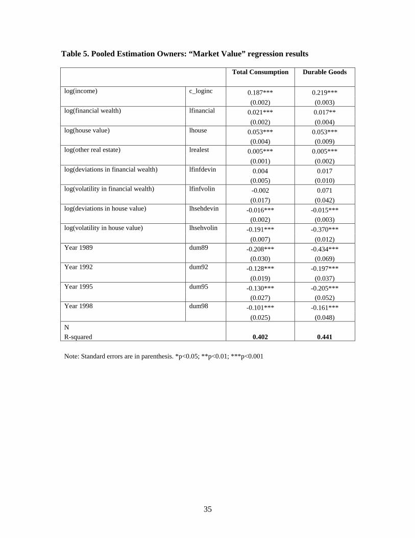
Table 5. Pooled Estimation Owners: “Market Value” regression results
Total Consumption Durable Goods
log(income) c_loginc 0.187*** 0.219*** (0.002) (0.003)
log(financial wealth) lfinancial 0.021*** 0.017** (0.002) (0.004)
log(house value) lhouse 0.053*** 0.053*** (0.004) (0.009)
log(other real estate) lrealest 0.005*** 0.005*** (0.001) (0.002)
log(deviations in financial wealth) lfinfdevin 0.004 0.017 (0.005) (0.010)
log(volatility in financial wealth) lfinfvolin -0.002 0.071 (0.017) (0.042)
log(deviations in house value) lhsehdevin -0.016*** -0.015*** (0.002) (0.003)
log(volatility in house value) lhsehvolin -0.191*** -0.370*** (0.007) (0.012)
Year 1989 dum89 -0.208*** -0.434*** (0.030) (0.069)
Year 1992 dum92 -0.128*** -0.197*** (0.019) (0.037)
Year 1995 dum95 -0.130*** -0.205*** (0.027) (0.052)
Year 1998 dum98 -0.101*** -0.161*** (0.025) (0.048)
N R-squared 0.402 0.441 Note: Standard errors are in parenthesis. *p<0.05; **p<0.01; ***p<0.001
35

36
Table 6. Credit-constrained Homeowners: Market value regression results 1989 1992 1995 1998 2001 Total Consumption
log(income) 0.109*** 0.132*** 0.255*** 0.163*** 0.135***
(0.024) (0.025) (0.030) (0.026) (0.020)
log(financial wealth) 0.027** 0.036*** 0.011 0.017 0.022*
(0.010) (0.009) (0.009) (0.011) (0.009)
log(house value) 0.072** 0.040 0.033 0.047 0.028
(0.026) (0.026) (0.028) (0.027) (0.023)
log(other real estate) 0.004 0.007 0.001 0.005 0.000
(0.006) (0.005) (0.005) (0.005) (0.005)
N 431 517 512 559 718
R-squared 0.408 0.418 0.411 0.346 0.293
Durable Goods log(income) 0.210*** 0.166*** 0.357*** 0.210*** 0.144***
(0.053) (0.047) (0.056) (0.041) (0.032)
log(financial wealth) 0.039 0.046** 0.011 0.014 0.028
(0.021) (0.017) (0.016) (0.018) (0.016)
log(house value) 0.093 0.059 -0.012 0.044 0.024
(0.057) (0.049) (0.052) (0.043) (0.038)
log(other real estate) 0.000 0.006 0.000 0.008 -0.006
(0.014) (0.010) (0.010) (0.008) (0.008)
N 431 517 512 559 718
R-squared 0.250 0.250 0.262 0.255 0.172
Note: Standard errors are in parenthesis. *p<0.05; **p<0.01; ***p<0.001

Appendix A. Variable Definitions
Variable Definition CEX Consumption Variables total consumption total annual spending on all goods and services durable goods annual spending on durable goods+ nondurable goods annual spending on nondurable goods
SCF Wealth Variables Market Value Financial wealth liquid and quasi-liquid financial assets including retirement and pensions house value estimated value of primary residence other real estate value estimated value of all real estate other than primary residence Net Wealth net wealth liquid and non-liquid financial assets minus financial debt home equity house value minus mortgages and home equity loans other real estate equity real estate value net of mortgages and equity loans
Interactive SCF Wealth Variables
Market Value lfinfdev interaction of log household financial wealth and current year deviation from
average of prior 3 years in Wilshire 5000 index lfinfvol interaction of log household financial wealth and volatility of Wilshire 5000
(as measured by standard deviation of Wilshire 5000 index over prior three years)
Lhsehdev interaction of log household house value and current year deviation from average of prior 3 years in regional OFHEO house price repeat sales index
lhsehvol interaction of log household house value and volatility of regional OFHEO repeat sales house price index (as measured by standard deviation of OFHEO index over the prior three years)
Net Wealth Nfinfdev interaction of net financial wealth and current year deviation from average of
prior 3 years in Wilshire 5000 index Nfinfvol interaction of net financial wealth and volatility of Wilshire 5000 (as
measured by standard deviation of Wilshire 5000 index over the prior three years)
Heqhdev interaction of home equity and current year deviation from average of prior 3 years in regional OFHEO house price repeat sales index
Heqhvol interaction of home equity and volatility of regional OFHEO repeat sale house price index (as measured by standard deviation of OFHEO index over the prior three years)
Categorical Matching Variables
race white, black, other race age age 25-35, age36-50, age 51-65 marital status married, not married education less than high school, high school, some college, college degree
37

Control Variables dum89 =1 if Year 1989 dum92 =1 if Year 1992 dum95 =1 if Year 1995 dum98 =1 if Year 1998 less than high school =1 if HOH’s highest education is less than high school diploma some college =1 if HOH’s highest education is some college college graduate =1 if HOH’s highest education is 4-year college degree family size number of family members living in household age 25-35 =1 if HOH’s age is 25-35 age 51-65 =1 if HOH’s age is 51-65 white =1 if HOH identifies race as white Black =1 if HOH identifies race as black northeast =1 if household in is in the Northeast south =1 if household in is in the South west =1 if household in is in the West married =1 if household is married divorced =1 if household is divorced separated =1 if household is separated widow =1 if household is widow
+ Durable goods are defined based on the U.S. Census Bureau’s Manufacturing, Mining, & Construction Statistics available at: http://www.census.gov/indicator/www/m3.
38

Appendix B. Homeowners: Market value regressions full results for ‘Total Consumption’
Total Consumption 1989 1992 1995 1998 2001
log (income) 0.162*** 0.198*** 0.188*** 0.197*** 0.191*** (0.012) (0.013) (0.012) (0.015) (0.012)
log (financial wealth) 0.021*** 0.024*** 0.023*** 0.018** 0.020*** (0.005) (0.005) (0.005) (0.006) (0.005)
log (house value) 0.060*** 0.050*** 0.050*** 0.046** 0.042*** (0.011) (0.013) (0.014) (0.016) (0.012)
log (other real estate value) 0.008*** 0.006** 0.006** 0.004 0.005* (0.002) (0.002) (0.002) (0.003) (0.002)
less than high school -0.124*** -0.069 -0.142*** -0.171*** -0.070 (0.034) (0.036) (0.039) (0.047) (0.041)
some college 0.034 0.097*** 0.092** 0.089** 0.104*** (0.028) (0.029) (0.029) (0.034) (0.028)
college graduate 0.163*** 0.187*** 0.211*** 0.216*** 0.259*** (0.029) (0.028) (0.029) (0.035) (0.028)
family size 0.054*** 0.048*** 0.054*** 0.043*** 0.059*** (0.008) (0.008) (0.008) (0.010) (0.008)
age 25-35 -0.068* -0.052* 0.018 -0.020 -0.028 (0.026) (0.027) (0.029) (0.034) (0.029)
age 51-65 -0.121*** -0.137*** -0.091*** -0.080* -0.121*** (0.026) (0.027) (0.027) (0.032) (0.025)
white 0.179*** 0.069 -0.049 0.095* 0.105** (0.041) (0.040) (0.039) (0.044) (0.035)
black 0.039 -0.046 -0.096 0.124* -0.025 (0.059) (0.055) (0.055) (0.062) (0.050)
northeast 0.018 0.109*** 0.102*** 0.098* 0.037 (0.029) (0.029) (0.031) (0.040) (0.032)
south -0.006 0.061* 0.029 -0.066* -0.022 (0.027) (0.028) (0.027) (0.033) (0.027)
west 0.164*** 0.140*** 0.088** 0.149*** 0.054 (0.029) (0.029) (0.030) (0.037) (0.029)
married 0.311*** 0.295*** 0.206*** 0.237*** 0.261*** (0.042) (0.047) (0.043) (0.052) (0.041)
divorced 0.120* 0.097 0.012 0.057 0.030 (0.050) (0.052) (0.049) (0.058) (0.046)
separated 0.251** 0.094 0.034 0.094 0.097 (0.078) (0.077) (0.096) (0.099) (0.090)
widow 0.161** 0.219** 0.075 0.109 0.157* (0.061) (0.072) (0.061) (0.081) (0.064)
N 2116 2033 1994 2097 2759 R-squared 0.401 0.433 0.418 0.337 0.376
Note: Standard errors are in parenthesis. *p<0.05; **p<0.01; ***p<0.001
39

Appendix C. Homeowners: Market value regressions full result for ‘Durable Goods’
Durable Goods 1989 1992 1995 1998 2001
log (income) 0.243*** 0.207*** 0.230*** 0.226*** 0.199*** (0.028) (0.024) (0.022) (0.023) (0.019)
log (financial wealth) 0.021 0.030*** 0.027** 0.018 0.020* (0.011) (0.009) (0.009) (0.009) (0.008)
log (house value) 0.076 ** 0.042 0.038 0.039 0.033 (0.026) (0.024) (0.025) (0.023) (0.021)
log (other real estate value) 0.008 0.006 0.006 0.006 0.002 (0.005) (0.004) (0.004) (0.004) (0.003)
less than high school -0.036 -0.202** -0.155* -0.144* -0.114 (0.078) (0.068) (0.071) (0.069) (0.065)
some college 0.171** 0.143** 0.126* 0.111* 0.138** (0.064) (0.054) (0.053) (0.049) (0.044)
college graduate 0.306*** 0.300*** 0.246*** 0.274*** 0.308*** (0.066) (0.053) (0.053) (0.052) (0.045)
family size 0.003 0.049** 0.050** 0.019 0.068*** (0.018) (0.015) (0.016) (0.015) (0.013)
age 25-35 0.145* 0.057 0.126* 0.120 0.077 (0.061) (0.050) (0.053) (0.050) (0.046)
age 51-65 -0.303*** -0.346*** -0.219*** -0.222*** -0.232*** (0.061) (0.051) (0.050) (0.047) (0.040)
white 0.246** -0.086 -0.096 -0.072 0.066 (0.094) (0.076) (0.071) (0.064) (0.056)
black 0.198 -0.156 -0.205* 0.151* -0.166* (0.135) (0.103) (0.101) (0.092) (0.080)
northeast -0.079 0.244*** 0.219*** 0.195*** 0.069 (0.067) (0.055) (0.056) (0.058) (0.051)
south -0.091 0.115* 0.059 -0.153** -0.073 (0.062) (0.052) (0.050) (0.049) (0.043)
west 0.258*** 0.334*** 0.264*** 0.271*** 0.101* (0.068) (0.055) (0.055) (0.054) (0.047)
Married 0.348*** 0.315*** 0.200* 0.301*** 0.235*** (0.096) (0.088) (0.079) (0.076) (0.065)
Divorced 0.083 0.145 0.098 0.102 0.113 (0.116) (0.098) (0.089) (0.085) (0.073)
Separated 0.218 0.173 0.066 0.139 0.132 (0.180) (0.145) (0.176) (0.146) (0.144)
Widow 0.207 0.162 0.059 -0.059 0.097 (0.140) (0.135) (0.112) (0.118) (0.102)
N 2116 2033 1994 2097 2759 R-squared 0.191 0.268 0.234 0.256 0.223
Note: Standard errors are in parenthesis. *p<0.05; **p<0.01; ***p<0.001
40

Appendix D. Homeowners: Net Wealth regression full results for ‘Total Consumption’
Total Consumption 1989 1992 1995 1998 2001 log (income) 0.194*** 0.236*** 0.219*** 0.225*** 0.219***
(0.011) (0.012) (0.012) (0.014) (0.011) net financial wealth (million $) 0.065** 0.026* 0.062*** 0.008 0.009*
(0.021) (0.010) (0.017) (0.005) (0.004) home equity (million $) 0.247*** 0.160*** 0.076* 0.096* 0.120**
(0.065) (0.048) (0.038) (0.047) (0.038) other real estate equity (million$) 0.011* 0.014* 0.024* 0.017 0.013
(0.005) (0.006) (0.012) (0.015) (0.012) less than high school -0.167*** -0.111** -0.209*** -0.203** -0.114**
(0.034) (0.036) (0.038) (0.047) (0.040) some college 0.050 0.126*** 0.120*** 0.110*** 0.121***
(0.028) (0.029) (0.029) (0.033) (0.027) college graduate 0.220*** 0.252*** 0.263*** 0.266*** 0.305***
(0.028) (0.027) (0.028) (0.034) (0.027) family size 0.054*** 0.047*** 0.053*** 0.043*** 0.059***
(0.008) (0.008) (0.009) (0.011) (0.008) age 25-35 -0.102*** -0.080** -0.039 -0.057 -0.066*
(0.026) (0.027) (0.028) (0.034) (0.029) age 51-65 -0.107*** -0.102*** -0.061* -0.054 -0.096***
(0.027) (0.027) (0.027) (0.031) (0.025) white 0.204*** 0.082* -0.040 0.107* 0.114**
(0.041) (0.041) (0.039) (0.044) (0.035) Black 0.003 -0.062 -0.138* 0.103 -0.036
(0.059) (0.056) (0.055) (0.063) (0.050) northeast 0.021 0.120*** 0.106*** 0.102* 0.038
(0.029) (0.030) (0.031) (0.040) (0.032) south 0.003 0.067* 0.028 -0.071* -0.023
(0.027) (0.028) (0.028) (0.033) (0.027) west 0.179*** 0.143*** 0.091** 0.014*** 0.055
(0.030) (0.030) (0.030) (0.037) (0.030) married 0.330*** 0.334*** 0.244*** 0.269*** 0.398***
(0.042) (0.047) (0.043) (0.052) (0.040) divorced 0.106* 0.102 0.009 0.064 0.041
(0.051) (0.053) (0.049) (0.058) (0.046) separated 0.226** 0.087 0.029 0.097 0.120
(0.079) (0.078) (0.097) (0.100) (0.091) widow 0.147* 0.234** 0.067 0.097 0.171**
(0.062) (0.073) (0.062) (0.081) (0.064) N 2116 2033 1994 2095 2700 R-squared 0.386 0.418 0.403 0.330 0.369
Note: Standard errors are in parenthesis. *p<0.05; **p<0.01; ***p<0.001
41

Appendix E. Homeowners: Net Wealth regression full results for ‘Durable Goods’
Durable Goods 1989 1992 1995 1998 2001 log (income) 0.284*** 0.250*** 0.262*** 0.254*** 0.227***
(0.026) (0.022) (0.021) (0.021) (0.017) net financial wealth (million $) 0.041 0.023 0.067* 0.007 -0.002
(0.048) (0.019) (0.031) (0.007) (0.006) home equity (million $) 0.233 0.124 0.030 0.099 0.107
(0.148) (0.088) (0.070) (0.068) (0.061) other real estate equity (million$)
0.019 0.016 0.037 0.009 -0.006 (0.010) (0.012) (0.022) (0.022) (0.019)
less than high school -0.092 -0.251*** -0.222** -0.176* -0.155* (0.078) (0.068) (0.069) (0.068) (0.064)
some college 0.193** 0.176** 0.152** 0.132** 0.155*** (0.064) (0.054) (0.053) (0.049) (0.044)
college graduate 0.384*** 0.374*** 0.293*** 0.320*** 0.353*** (0.063) (0.050) (0.051) (0.049) (0.043)
family size 0.033 0.048** 0.049** 0.019 0.068*** (0.018) (0.015) (0.016) (0.015) (0.013)
age 25-35 0.105 0.025 0.070 0.082 0.043 (0.060) (0.050) (0.052) (0.049) (0.046)
age 51-65 -0.281*** -0.300*** -0.188*** -0.194*** -0.205*** (0.061) (0.050) (0.049) (0.046) (0.040)
white 0.270** -0.066 -0.084 -0.061 0.079 (0.094) (0.076) (0.071) (0.064) (0.056)
Black 0.152 -0.169 -0.244* 0.131 -0.176* (0.135) (0.103) (0.100) (0.092) (0.080)
northeast -0.075 0.258*** 0.222*** 0.199*** 0.071 (0.067) (0.056) (0.056) (0.058) (0.052)
south -0.085 0.121* 0.059 -0.157** -0.073 (0.062) (0.052) (0.050) (0.049) (0.043)
west 0.277*** 0.338*** 0.268*** 0.269*** 0.104* (0.068) (0.055) (0.055) (0.054) (0.047)
married 0.368*** 0.358*** 0.236** 0.329*** 0.263*** (0.096) (0.088) (0.079) (0.076) (0.064)
divorced 0.069 0.150 0.095 0.108 0.122 (0.116) (0.099) (0.090) (0.085) (0.073)
separated 0.187 0.164 0.061 0.143 0.149 (0.181) (0.146) (0.176) (0.146) (0.144)
Widow 0.188 0.176 0.052 -0.071 0.109 (0.141) (0.136) (0.112) (0.119) (0.102)
N 2116 2033 1994 2095 2700 R-squared 0.185 0.260 0.229 0.252 0.220
Note: Standard errors are in parenthesis. *p<0.05; **p<0.01; ***p<0.001
42

Appendix F: Pooled Estimation Full Regression Results “Market Value” for Homeowners
Total
Consumption Durable Goods
log(income) c_loginc 0.187*** 0.219*** (0.002) (0.003)
log (financial wealth) lfinancial 0.021*** 0.017** (0.002) (0.004)
log (house value) lhouse 0.053*** 0.053*** (0.004) (0.009)
log(other real estate) lrealest 0.005*** 0.005*** (0.001) (0.002)
log (deviations in financial wealth) lfinfdevin 0.004 0.017 (0.005) (0.010)
log (volatility in financial wealth) lfinfvolin -0.002 0.071 (0.017) (0.042)
log (deviations in house value) lhsehdevin -0.016*** -0.015*** (0.002) (0.003)
log (volatility in house value) lhsehvolin -0.191*** -0.370*** (0.007) (0.012)
Year 1989 dum89 -0.208*** -0.434*** (0.030) (0.069)
Year 1992 dum92 -0.128*** -0.197*** (0.019) (0.037)
Year 1995 dum95 -0.130*** -0.205*** (0.027) (0.052)
Year 1998 dum98 -0.101*** -0.161*** (0.025) (0.048)
less than high school nodip -0.118*** -0.136*** (0.018) (0.031)
some college somecoll 0.084*** 0.136*** (0.013) (0.023)
college graduate badegree 0.214*** 0.289*** (0.013) (0.024)
family size famsize 0.051*** 0.044*** (0.004) (0.007)
age 25-35 age2535 -0.033* 0.106*** (0.013) (0.023)
age 51-65 age5065 -0.112*** -0.264*** (0.012) (0.022)
white white 0.079*** 0.014 (0.018) (0.031)
black black -0.001 -0.048 (0.025) (0.044)
northeast northeast 0.093*** 0.172*** (0.015) (0.027)
south south -0.014 -0.050* (0.013) (0.023)
43

44
west west 0.144*** 0.295*** (0.016) (0.029)
married married 0.262*** 0.277*** (0.020) (0.036)
divorced divorced 0.058* 0.115* (0.023) (0.041)
separated separated 0.113** 0.151* (0.039) (0.070)
widow widow 0.139*** 0.101 (0.030) (0.054)
N 10,938 10,938 R-squared 0.402 0.441 Note: Standard errors are in parenthesis. *p<0.05; **p<0.01; ***p<0.001