Embed Size (px)
Citation preview
FEDERAL RESERVE BANK OF SAN FRANCISCO
WORKING PAPER SERIES
House Prices, Expectations, and Time-Varying Fundamentals
Paolo Gelain Norges Bank
Kevin J. Lansing
Federal Reserve Bank of San Francisco
May 2014
The views in this paper are solely the responsibility of the authors and should not be interpreted as reflecting the views of the Federal Reserve Bank of San Francisco or the Board of Governors of the Federal Reserve System.
Working Paper 2013-03 http://www.frbsf.org/publications/economics/papers/2013/wp2013-03.pdf
House Prices, Expectations, and Time-Varying Fundamentals∗
Paolo Gelain†
Norges Bank
Kevin J. Lansing‡
Federal Reserve Bank of San Francisco
May 7, 2014
Abstract
We investigate the behavior of the equilibrium price-rent ratio for housing in a standard
asset pricing model and compare the model predictions to survey evidence on the return
expectations of real-world housing investors. We allow for time-varying risk aversion (via
external habit formation) and time-varying persistence and volatility in the stochastic
process for rent growth, consistent with U.S. data for the period 1960 to 2013. Under
fully-rational expectations, the model significantly underpredicts the volatility of the U.S.
price-rent ratio for reasonable levels of risk aversion. We demonstrate that the model can
approximately match the volatility of the price-rent ratio in the data if near-rational agents
continually update their estimates for the mean, persistence and volatility of fundamental
rent growth using only recent data (i.e., the past 4 years), or if agents employ a simple
moving-average forecast rule for the price-rent ratio that places a large weight on the
most recent observation. These two versions of the model can be distinguished by their
predictions for the correlation between expected future returns on housing and the price-
rent ratio. Only the moving-average model predicts a positive correlation such that agents
tend to expect high future returns when prices are high relative to fundamentals–a feature
that is consistent with a wide variety of survey evidence from real estate and stock markets.
Keywords: Asset pricing, Excess volatility, Housing bubbles, Predictability, Time-varying
risk premiums, Expected returns.
JEL Classification: D84, E32, E44, G12, O40, R31.
∗Forthcoming, Journal of Empirical Finance. For helpful comments and suggestions, we would like to
thank colleagues at the Norges Bank, Lars Løchstøer, Tassos Malliaris, and seminar participants at Carleton
University, the 2012 Meeting of the Society for Computational Economics, the 2012 Symposium of the Society
for Nonlinear Dynamics and Econometrics, the 2012 Meeting of the European Economics Association, the
2013 Meeting of the American Economics Association, the 2013 Arne Ryde Workshop in Financial Economics
hosted by Lund University, and the 2013 BMRC-QASS Conference on Macro and Financial Economics, hosted
by the Brunel Macroeconomics Research Centre. We would also like to thank two anonymous referees for
comments that significantly improved the paper. Part of this research was conducted while Lansing was a
visiting economist at the Norges Bank, whose hospitality is gratefully acknowledged.†Norges Bank, P.O. Box 1179, Sentrum, 0107 Oslo, email: [email protected]‡Corresponding author. Federal Reserve Bank of San Francisco, P.O. Box 7702, San Francisco, CA 94120-
7702, email: [email protected]
1 Introduction
1.1 Overview
House prices in the United States increased dramatically in the years prior to 2007. During the
boom years, many economists and policymakers argued that a bubble did not exist and that
numerous fundamental factors were driving the run-up in prices.1 But in retrospect, many
studies now attribute the run-up to a classic bubble driven by over-optimistic projections
about future house price growth which, in turn, led to a collapse in lending standards.2 Rem-
iniscent of the U.S. stock market mania of the late-1990s, the mid-2000s housing market was
characterized by an influx of unsophisticated buyers and record transaction volume. When the
optimistic house price projections eventually failed to materialize, the bubble burst, setting
off a chain of events that led to a financial and economic crisis. The “Great Recession,” which
started in December 2007 and ended in June 2009, was the most severe economic contraction
since 1947, as measured by the peak-to-trough decline in real GDP (Lansing 2011).
This paper investigates the behavior of the equilibrium price-rent ratio for housing in
a standard Lucas-type asset pricing model and compares the model predictions to survey
evidence on the return expectations of real-world housing investors. We allow for time-varying
risk aversion (via external habit formation) and time-varying persistence and volatility in the
stochastic process for rent growth, consistent with U.S. data for the period 1960 to 2013.
Under fully-rational expectations, the model significantly underpredicts the volatility of the
U.S. price-rent ratio for reasonable levels of risk aversion. We demonstrate that the model can
approximately match the volatility of the price-rent ratio in the data if near-rational agents
continually update their estimates for the mean, persistence and volatility of fundamental rent
growth using only recent data (i.e., the past 4 years), or if agents employ a simple moving-
average forecast rule for the price-rent ratio that places a large weight on the most recent
observation. These two versions of the model can be distinguished by their predictions for
the correlation between expected future returns on housing and the price-rent ratio. Only
the moving-average model predicts a positive correlation such that agents tend to expect high
future returns when prices are high relative to fundamentals–a feature that is consistent with
a wide variety of survey evidence from real estate and stock markets.3
1See, for example, McCarthy and Peach (2004) and Himmelberg, et al. (2005). In an October 2004 speech,
Fed Chairman Alan Greenspan (2004) argued that there were “significant impediments to speculative trading”
in the housing market that served as “an important restraint on the development of price bubbles.” In a July 1,
2005 media interview, Ben Bernanke, then Chairman of the President’s Council of Economic Advisers, asserted
that fundamental factors such as strong growth in jobs and incomes, low mortgage rates, demographics, and
restricted supply were supporting U.S. house prices. In the same interview, Bernanke stated his view that a
substantial nationwide decline in house prices was “a pretty unlikely possibility.” For additional details, see
Jurgilas and Lansing (2013).2For a comprehensive review of events, see the report of the U.S. Financial Crisis Inquiry Commission (2011).
Recently, in a review of the Fed’s forecasting record leading up to the crisis, Potter (2011) acknowledges a
“misunderstanding of the housing boom. . . [which] downplayed the risk of a substantial fall in house prices.”3The survey evidence on expected returns is discussed in more detail in the next section. For an overview
the evidence, see Williams (2013).
1
As part of our quantitative analysis, we apply the Campbell and Shiller (1988) log-linear
approximation of the return identity to the housing market. According to this identity, the
variance of the log price-rent ratio must equal the sum of the ratio’s covariances with: (1)
future rent growth rates, and (2) future realized housing returns. The magnitude of each
covariance term is a measure of the predictability of future rent growth or future realized
returns when the current price-rent ratio is employed as the sole regressor in a forecasting
equation. As in the U.S. data, the moving-average model exhibits the property that a higher
price-rent ratio in the current period strongly predicts lower realized returns in the future,
but the predictive power for future rent growth is very weak. Interestingly, even though a
higher price-rent ratio in the data predicts lower realized returns, the survey evidence shows
that real-world investors fail to take this relationship into account; instead they continue to
forecast high future returns following a sustained run-up in the price-rent ratio. Such behavior
is consistent with a moving-average forecast rule but is inconsistent with the fully-rational and
near-rational versions of the model.
We also show that the moving-average model can deliver either a positive or negative
regression coefficient on the price-rent ratio when the ratio is used to predict future rent growth.
The sign of the regression coefficient is influenced by the value of a utility curvature parameter.
Our simulation results can therefore help account for the empirical findings of Engsted and
Pedersen (2012), who document significant cross-country and sub-sample instability in the
sign of this regression coefficient using housing market data from 18 OECD countries over the
period 1970 to 2011.
An additional contribution of the paper is to derive an approximate analytical solution for
the fully-rational house price in the case when fundamental rent growth exhibits time-varying
persistence and volatility. Our specification for rent growth employs the bilinear time series
model originally developed Granger and Andersen (1978) which allows for nonlinear behavior
within a continuous state space. Our solution procedure makes use of a change of variables to
preserve as much of the model’s nonlinear characteristics as possible.
Standard dynamic stochastic general-equilibrium (DSGE) models with fully-rational ex-
pectations have difficulty producing large swings in house prices that resemble the patterns
observed in the U.S. and other countries over the past decade. Indeed, it is common for such
models to postulate extremely large and persistent exogenous shocks to rational agents’ pref-
erences for housing in an effort to bridge the gap between the model and the data.4 Leaving
aside questions about where these preference shocks actually come from and how agents’ re-
sponses to them could become coordinated, we demonstrate numerically that an upward shift
in the representative agent’s preference for housing raises the mean price-rent ratio under all
three expectations regimes. At the same time, the preference shift lowers the average realized
return on housing. Under rational expectations, the agent will take this relationship into ac-
count when forecasting such that the conditional expected future return on housing will move
4See for example, Iacoviello and Neri (2010), among others.
2
in the opposite direction as the price-rent ratio in response to a shift in housing preferences.
Hence, while a fully-rational model with housing preference shocks could potentially match
the volatility of the price-rent ratio in the data, such a model would still predict a negative
correlation between the expected future return on housing and the price-rent ratio–directly at
odds with the survey evidence to be described in section 2. Moreover, since preference shocks
influence the utility dividend, or “imputed rent” received from housing, a preference-driven
run-up in house prices would be accompanied by an increase in the imputed rent–something
which is not observed in U.S. data during the boom years of the mid-2000s.
1.2 Related Literature
Numerous empirical studies starting with Shiller (1981) and LeRoy and Porter (1981) have
shown that stock prices appear to exhibit excess volatility when compared to the discounted
stream of ex post realized dividends.5 Similarly, Campbell, et al. (2009) find that movements
in U.S. house price-rent ratios cannot be fully explained by movements in subsequent rent
growth.
A large body of research seeks to explain asset price behavior using some type of distorted
belief mechanism or misspecified forecast rule in a representative agent framework. Examples
along these lines include Barsky and Delong (1993), Timmerman (1996), Barberis, Shleifer,
and Vishney (1998), Lansing (2006, 2010), Adam, Marcet, and Nicolini (2008), Branch and
Evans (2010), Fuster, et al. (2012), and Hommes and Zhu (2014), among others.
An empirical study by Chow (1989) finds that an asset pricing model with adaptive expec-
tations outperforms one with rational expectations in accounting for observed movements in
U.S. stock prices and interest rates. Huh and Lansing (2000) show that a model with backward-
looking expectations is better able to capture the temporary rise in long-term nominal interest
rates observed in U.S. data at the start of the Volcker disinflation in the early-1980s. Some
recent research that incorporates moving-average forecast rules or adaptive expectations into
otherwise standard models include Sargent (1999, Chapter 6), Evans and Ramey (2006), Lans-
ing (2009), and Huang, et. al (2009), among others. Huang, et al. (2009) state that “adaptive
expectations can be an important source of frictions that amplify and propagate technology
shocks and seem promising for generating plausible labor market dynamics.”
Coibion and Gorodnichencko (2012) find robust evidence against full-information rational
expectations in survey forecasts for U.S. inflation and unemployment. Using an estimated New
Keynesian DSGE model, Levine, et al. (2012) find that the fraction of agents who employ
a moving-average type forecast rule lies in the range of 0.65 to 0.83. Gelain, et al. (2013)
show that the introduction of simple moving-average forecast rules for a subset of agents can
significantly magnify the volatility and persistence of house prices and household debt in a
standard DSGE model with housing. Granziera and Kozicki (2012) show that a simple Lucas-
type asset pricing model with backward-looking, extrapolative-type expectations can roughly
5Lansing and LeRoy (2014) provide a recent update on this literature.
3
match the run-up in U.S. house prices from 2000 to 2006 as well as the subsequent sharp
downturn.
Constant-gain learning algorithms of the type described by Evans and Honkapoja (2001)
are similar in many respects to moving-average expectations; both formulations assume that
agents apply exponentially-declining weights to past data when constructing forecasts of future
variables. Adam, et al. (2012) show that the introduction of constant-gain learning can help
account for recent cross-country patterns in house prices and current account dynamics. In
contrast to our setup, their model assumes the presence of volatile and persistent exogenous
shocks to the representative agent’s preference for housing services, a feature that helps their
model to fit the data. A strength of their model is that it takes into account the positive
supply response of residential construction to rising house prices–a feature that is evident
in most historical real estate booms (Shiller 2008). When the new housing supply becomes
available with a lag, it can reinforce an expectation-driven decline in house prices.
There is also a large literature on “rational bubbles” in which agents are fully cognizant of
the fundamental asset price, but nevertheless are willing to pay more than this amount. This
can occur if expectations of future price appreciation are large enough to satisfy the rational
agent’s required rate of return.6 A drawback of rational bubble models is the prediction that
the equilibrium price-dividend ratio (or price-rent ratio) has a unit root. A more elaborate
version assumes that the rational bubble will periodically crash according to some universally-
known probability function (Evans 1991), but this is an ad hoc feature that is determined
completely outside of the model. Recently, Doblas-Madrid (2012) develops a model with
only rational agents who ride bubbles while optimally weighing potential profits if they can
successfully time the market versus the potential losses if the bubble bursts before they can sell.
In his model, price run-ups relative to fundamentals can coincide with the speculators’ rational
expectations of higher future profits for an extended period, a feature which is consistent with
the survey evidence.
2 Evidence on Investor Expectations
The fundamental value of an asset is typically measured by the present-value of expected
future cash or service flows that will accrue to the owner. Service flows from housing are
called “imputed rents.” The discount rate used in the present-value calculation is comprised of
a risk-free yield and a compensation for perceived risk, i.e., a risk premium. Their sum defines
the rate of return that an investor expects to receive to justify purchase of the asset. All else
equal, a lower risk premium implies a lower expected return and a lower discount rate in the
present-value calculation. Future service flows will be discounted less and the fundamental
value will rise.
6Lansing (2010) derives a continuum of rational bubble solutions in a standard Lucas-type asset pricing
model.
4
Making use of the above logic, Cochrane (2011) argues that one cannot easily tell the
difference between a bubble and a situation where rational investors have low risk premia,
implying lower expected returns on the risky asset. Specifically, he remarks “Crying bubble
is empty unless you have an operational procedure for distinguishing them from rationally
low risk premiums.” Along similar lines, Favilukis, et al. (2013) argue that the run-up in
U.S. house prices relative to rents was largely due to a financial market liberalization (easier
lending standards and lower mortgage transaction costs) that reduced buyers’ perceptions of
the riskiness of housing assets. In the words of the authors, “a financial market liberaliza-
tion drives price-rent ratios up because it drives risk premia down. . . Procyclical increases in
[fundamental] price-rent ratios reflect rational expectations of lower future returns.”
In our view, the relaxation of lending standards in the mid-2000s was an endogenous
consequence of the house price run-up, not an exogenous fundamental driver of the run-
up. Standards were relaxed because lenders (and willing borrowers) expected house price
appreciation to continue indefinitely. Empirical evidence supports this view. Within the
United States, past house price appreciation in a given area had a significant positive influence
on subsequent loan approval rates in the same area (Dell’Ariccia, et al. 2012, Goetzmann, et
al. 2012).
One way in which a bubble might be distinguished from a situation with rationally low risk
premiums is to examine investors’ expectations about future returns on the asset. Rational
investors with low risk premiums would expect low future returns after a sustained price
run-up, whereas irrationally exuberant investors in the midst of a bubble would expect high
future returns because they simply extrapolate recent price action into the future. Survey
data from both real estate and stock markets show that real-world investors typically expect
high future returns near market peaks, not low future returns. Overall, the survey evidence
directly contradicts the view that declining risk premiums (resulting in low expected returns)
were the explanation for the run-up in U.S. house prices relative to rents.
In a study of data from the Michigan Survey of Consumers, Piazzesi and Schneider (2009)
report that “starting in 2004, more and more households became optimistic after having
watched house prices increase for several years.” In a review of the time series evidence on
housing investor expectations from 2002 to 2008, Case, Shiller, and Thompson (2012) conclude
(p. 282) that “1-year expectations [of future house prices changes] are fairly well described as
attenuated versions of lagged actual 1-year price changes.”
Anecdotal evidence further supports the view that U.S. housing investors had high expected
returns near the market peak. The June 6, 2005 cover of Fortune magazine was titled “Real
Estate Gold Rush–Inside the hot-money world of housing speculators, condo-flippers and
get-rich-quick schemers.” One week later, the June 13, 2005 cover of Time magazine was titled
“Home $weet Home–Why we’re going gaga over real estate.” Both covers depicted happy and
celebrating housing investors–all suggesting a rosy outlook for U.S. real estate.
With regard to the stock market, studies by Fischer and Statman (2002), Vissing-Jorgenson
5
50
100
150
200
250
300
350
400
90 00 10 20 30 40 50 60 70 80 90 00 10
Norway
U.S.
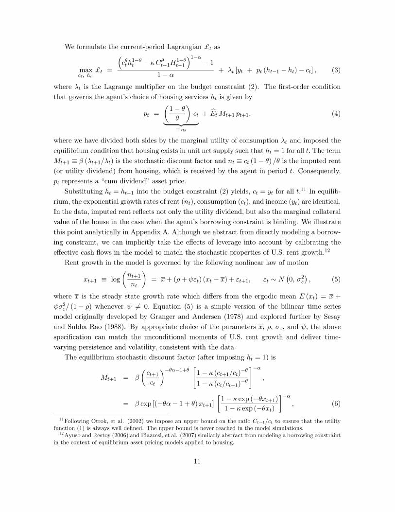
Real House Price Indices: 1890 to 2013
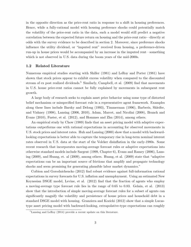
Figure 1: Long-run real house price indices for U.S. and Norway. Periods of stagnant real
house prices are interspersed with booms and busts. Norway experienced a major housing
price boom in the late 1980s followed by a crash in the early 1990s. The earlier boom-bust
pattern in Norway is similar in magnitude to the recent boom-bust pattern in U.S. house
prices. Real house prices are indexed to 100 in 1890.
(2004) and Amromin and Sharpe (2014) all find evidence of extrapolative or procyclical ex-
pected returns among investors. Recently, in a comprehensive study of the expectations of U.S.
stock market investors using survey data from a variety of sources, Greenwood and Shleifer
(2013) find that measures of investor expectations about future stock returns are positively
correlated with (1) the price-dividend ratio, (2) past stock returns, and (3) investor inflows
into mutual funds. They conclude (p. 30) that “[O]ur evidence rules out rational expecta-
tions models in which changes in market valuations are driven by the required returns of a
representative investor...Future models of stock market fluctuations should embrace the large
fraction of investors whose expectations are extrapolative.” We apply their advice here to a
model of housing market fluctuations.
3 Housing Market Data
Figure 1 plots real house price indices in the U.S. and Norway from 1890 to 2013. The U.S.
data are updated from Shiller (2005) while data for Norway are updated from Eitrheim and
Erlandsen (2004, 2005). Both series show that real house prices were relatively stagnant for
6
80
120
160
200
240
280
320
360
60 65 70 75 80 85 90 95 00 05 10
Norway
U.S.
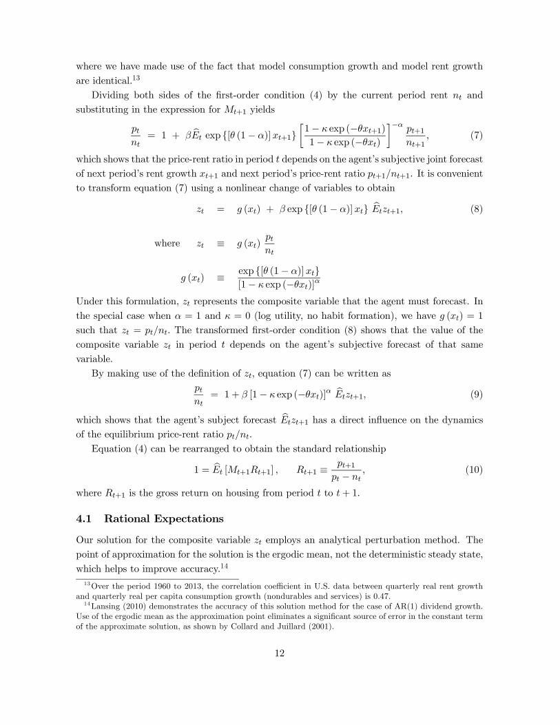
Price-Rent Indices: 1960 to 2013
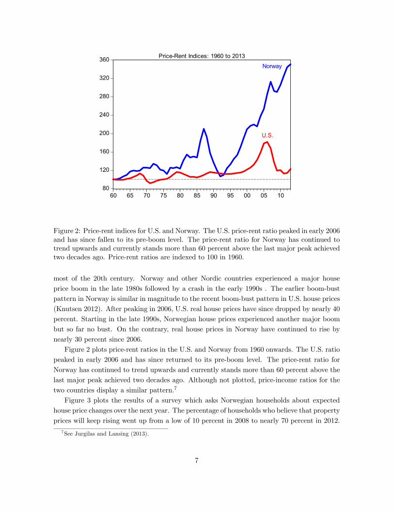
Figure 2: Price-rent indices for U.S. and Norway. The U.S. price-rent ratio peaked in early 2006
and has since fallen to its pre-boom level. The price-rent ratio for Norway has continued to
trend upwards and currently stands more than 60 percent above the last major peak achieved
two decades ago. Price-rent ratios are indexed to 100 in 1960.
most of the 20th century. Norway and other Nordic countries experienced a major house
price boom in the late 1980s followed by a crash in the early 1990s . The earlier boom-bust
pattern in Norway is similar in magnitude to the recent boom-bust pattern in U.S. house prices
(Knutsen 2012). After peaking in 2006, U.S. real house prices have since dropped by nearly 40
percent. Starting in the late 1990s, Norwegian house prices experienced another major boom
but so far no bust. On the contrary, real house prices in Norway have continued to rise by
nearly 30 percent since 2006.
Figure 2 plots price-rent ratios in the U.S. and Norway from 1960 onwards. The U.S. ratio
peaked in early 2006 and has since returned to its pre-boom level. The price-rent ratio for
Norway has continued to trend upwards and currently stands more than 60 percent above the
last major peak achieved two decades ago. Although not plotted, price-income ratios for the
two countries display a similar pattern.7
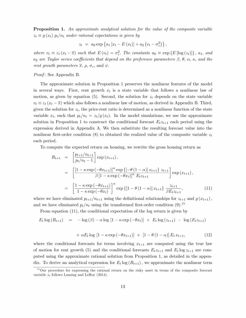
Figure 3 plots the results of a survey which asks Norwegian households about expected
house price changes over the next year. The percentage of households who believe that property
prices will keep rising went up from a low of 10 percent in 2008 to nearly 70 percent in 2012.
7See Jurgilas and Lansing (2013).
7
0
10
20
30
40
50
60
70
80
2007 2008 2009 2010 2011 2012
% expecting an increase
% expecting a decrease
%
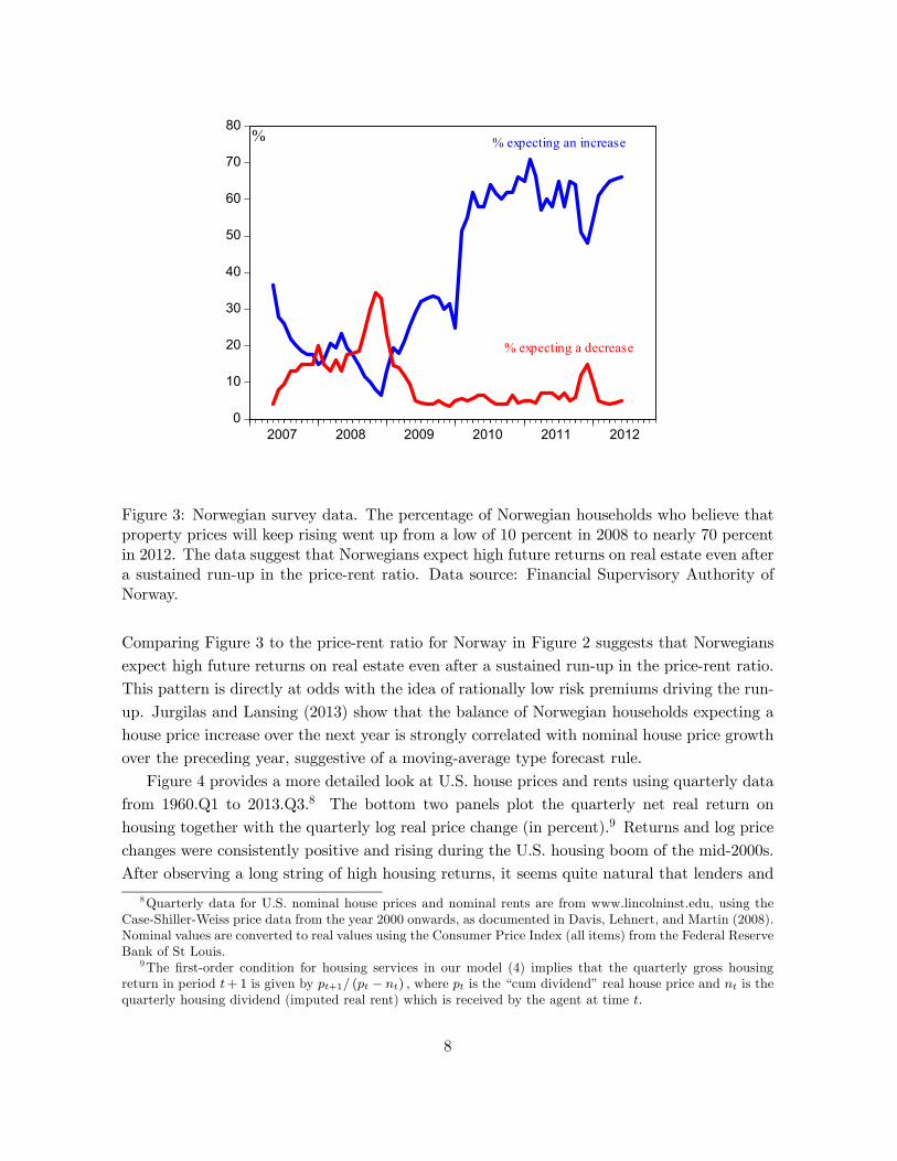
Figure 3: Norwegian survey data. The percentage of Norwegian households who believe that
property prices will keep rising went up from a low of 10 percent in 2008 to nearly 70 percent
in 2012. The data suggest that Norwegians expect high future returns on real estate even after
a sustained run-up in the price-rent ratio. Data source: Financial Supervisory Authority of
Norway.
Comparing Figure 3 to the price-rent ratio for Norway in Figure 2 suggests that Norwegians
expect high future returns on real estate even after a sustained run-up in the price-rent ratio.
This pattern is directly at odds with the idea of rationally low risk premiums driving the run-
up. Jurgilas and Lansing (2013) show that the balance of Norwegian households expecting a
house price increase over the next year is strongly correlated with nominal house price growth
over the preceding year, suggestive of a moving-average type forecast rule.
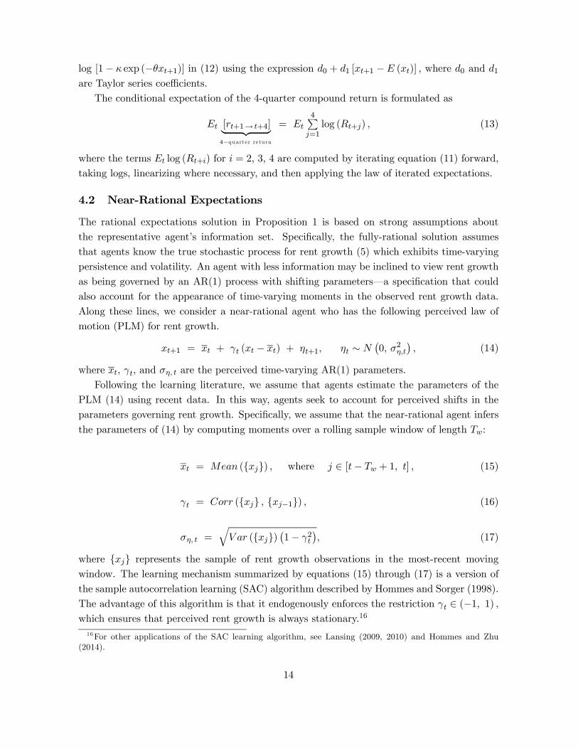
Figure 4 provides a more detailed look at U.S. house prices and rents using quarterly data
from 1960.Q1 to 2013.Q3.8 The bottom two panels plot the quarterly net real return on
housing together with the quarterly log real price change (in percent).9 Returns and log price
changes were consistently positive and rising during the U.S. housing boom of the mid-2000s.
After observing a long string of high housing returns, it seems quite natural that lenders and
8Quarterly data for U.S. nominal house prices and nominal rents are from www.lincolninst.edu, using the
Case-Shiller-Weiss price data from the year 2000 onwards, as documented in Davis, Lehnert, and Martin (2008).
Nominal values are converted to real values using the Consumer Price Index (all items) from the Federal Reserve
Bank of St Louis.9The first-order condition for housing services in our model (4) implies that the quarterly gross housing
return in period +1 is given by +1 ( − ) where is the “cum dividend” real house price and is the
quarterly housing dividend (imputed real rent) which is received by the agent at time
8
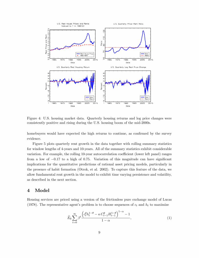
Figure 4: U.S. housing market data. Quarterly housing returns and log price changes were
consistently positive and rising during the U.S. housing boom of the mid-2000s.
homebuyers would have expected the high returns to continue, as confirmed by the survey
evidence.
Figure 5 plots quarterly rent growth in the data together with rolling summary statistics
for window lengths of 4-years and 10-years. All of the summary statistics exhibit considerable
variation. For example, the rolling 10-year autocorrelation coefficient (lower left panel) ranges
from a low of −017 to a high of 0.75. Variation of this magnitude can have significant
implications for the quantitative predictions of rational asset pricing models, particularly in
the presence of habit formation (Otrok, et al. 2002). To capture this feature of the data, we
allow fundamental rent growth in the model to exhibit time varying persistence and volatility,
as described in the next section.
4 Model
Housing services are priced using a version of the frictionless pure exchange model of Lucas
(1978). The representative agent’s problem is to choose sequences of and to maximize
b0 ∞X=0
³
1− −
−11−−1´1−
− 11−
(1)
9
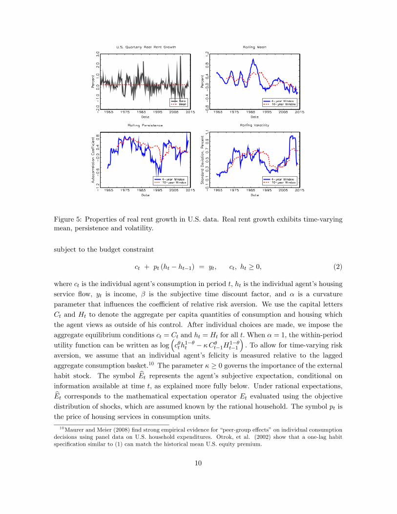
Figure 5: Properties of real rent growth in U.S. data. Real rent growth exhibits time-varying
mean, persistence and volatility.
subject to the budget constraint
+ ( − −1) = ≥ 0 (2)
where is the individual agent’s consumption in period is the individual agent’s housing
service flow, is income, is the subjective time discount factor, and is a curvature
parameter that influences the coefficient of relative risk aversion. We use the capital letters
and to denote the aggregate per capita quantities of consumption and housing which
the agent views as outside of his control. After individual choices are made, we impose the
aggregate equilibrium conditions = and = for all When = 1 the within-period
utility function can be written as log³
1− −
−11−−1´ To allow for time-varying risk
aversion, we assume that an individual agent’s felicity is measured relative to the lagged
aggregate consumption basket.10 The parameter ≥ 0 governs the importance of the externalhabit stock. The symbol b represents the agent’s subjective expectation, conditional on
information available at time as explained more fully below. Under rational expectations,b corresponds to the mathematical expectation operator evaluated using the objective
distribution of shocks, which are assumed known by the rational household. The symbol is
the price of housing services in consumption units.
10Maurer and Meier (2008) find strong empirical evidence for “peer-group effects” on individual consumption
decisions using panel data on U.S. household expenditures. Otrok, et al. (2002) show that a one-lag habit
specification similar to (1) can match the historical mean U.S. equity premium.
10
We formulate the current-period Lagrangian £ as
max
£ =
³
1− −
−11−−1´1−
− 11−
+ [ + (−1 − )− ] (3)
where is the Lagrange multiplier on the budget constraint (2). The first-order condition
that governs the agent’s choice of housing services is given by
=
µ1−
¶| {z }
≡
+ b+1 +1 (4)
where we have divided both sides by the marginal utility of consumption and imposed the
equilibrium condition that housing exists in unit net supply such that = 1 for all The term
+1 ≡ (+1) is the stochastic discount factor and ≡ (1− ) is the imputed rent
(or utility dividend) from housing, which is received by the agent in period . Consequently,
represents a “cum dividend” asset price.
Substituting = −1 into the budget constraint (2) yields, = for all 11 In equilib-
rium, the exponential growth rates of rent (), consumption (), and income () are identical.
In the data, imputed rent reflects not only the utility dividend, but also the marginal collateral
value of the house in the case when the agent’s borrowing constraint is binding. We illustrate
this point analytically in Appendix A. Although we abstract from directly modeling a borrow-
ing constraint, we can implicitly take the effects of leverage into account by calibrating the
effective cash flows in the model to match the stochastic properties of U.S. rent growth.12
Rent growth in the model is governed by the following nonlinear law of motion
+1 ≡ log
µ+1
¶= + (+ ) ( − ) + +1 ∼
¡0 2
¢ (5)
where is the steady state growth rate which differs from the ergodic mean () = +
2 (1− ) whenever 6= 0 Equation (5) is a simple version of the bilinear time series
model originally developed by Granger and Andersen (1978) and explored further by Sesay
and Subba Rao (1988). By appropriate choice of the parameters and the above
specification can match the unconditional moments of U.S. rent growth and deliver time-
varying persistence and volatility, consistent with the data.
The equilibrium stochastic discount factor (after imposing = 1) is
+1 =
µ+1
¶−−1+ "1− (+1)
−
1− (−1)−
#−
= exp [(−− 1 + )+1]
∙1− exp (−+1)1− exp (−)
¸− (6)
11Following Otrok, et al. (2002) we impose an upper bound on the ratio −1 to ensure that the utilityfunction (1) is always well defined. The upper bound is never reached in the model simulations.12Ayuso and Restoy (2006) and Piazzesi, et al. (2007) similarly abstract from modeling a borrowing constraint
in the context of equilibrium asset pricing models applied to housing.
11
where we have made use of the fact that model consumption growth and model rent growth
are identical.13
Dividing both sides of the first-order condition (4) by the current period rent and
substituting in the expression for +1 yields
= 1 + b exp {[ (1− )]+1}
∙1− exp (−+1)1− exp (−)
¸−+1
+1 (7)
which shows that the price-rent ratio in period depends on the agent’s subjective joint forecast
of next period’s rent growth +1 and next period’s price-rent ratio +1+1. It is convenient
to transform equation (7) using a nonlinear change of variables to obtain
= () + exp {[ (1− )]} b+1 (8)
where ≡ ()
() ≡ exp {[ (1− )]}[1− exp (−)]
Under this formulation, represents the composite variable that the agent must forecast. In
the special case when = 1 and = 0 (log utility, no habit formation), we have () = 1
such that = The transformed first-order condition (8) shows that the value of the
composite variable in period depends on the agent’s subjective forecast of that same
variable.
By making use of the definition of equation (7) can be written as
= 1 + [1− exp (−)] b+1 (9)
which shows that the agent’s subject forecast b+1 has a direct influence on the dynamics
of the equilibrium price-rent ratio .
Equation (4) can be rearranged to obtain the standard relationship
1 = b [+1+1] +1 ≡ +1
− (10)
where +1 is the gross return on housing from period to + 1
4.1 Rational Expectations
Our solution for the composite variable employs an analytical perturbation method. The
point of approximation for the solution is the ergodic mean, not the deterministic steady state,
which helps to improve accuracy.14
13Over the period 1960 to 2013, the correlation coefficient in U.S. data between quarterly real rent growth
and quarterly real per capita consumption growth (nondurables and services) is 0.47.14Lansing (2010) demonstrates the accuracy of this solution method for the case of AR(1) dividend growth.
Use of the ergodic mean as the approximation point eliminates a significant source of error in the constant term
of the approximate solution, as shown by Collard and Juillard (2001).
12
Proposition 1. An approximate analytical solution for the value of the composite variable
≡ () under rational expectations is given by
= 0 exp©1 [ − ()] + 2
¡ − 2
¢ª
where ≡ ( − ) such that () = 2 The constants 0 ≡ exp { [log ()]} 1 and2 are Taylor series coefficients that depend on the preference parameters and the
rent growth parameters and
Proof : See Appendix B.
The approximate solution in Proposition 1 preserves the nonlinear features of the model
in several ways. First, rent growth is a state variable that follows a nonlinear law of
motion, as given by equation (5). Second, the solution for depends on the state variable
≡ ( − ) which also follows a nonlinear law of motion, as derived in Appendix B. Third,
given the solution for , the price-rent ratio is determined as a nonlinear function of the state
variable such that = (). In the model simulations, we use the approximate
solution in Proposition 1 to construct the conditional forecast +1 each period using the
expression derived in Appendix A. We then substitute the resulting forecast value into the
nonlinear first-order condition (8) to obtained the realized value of the composite variable
each period.
To compute the expected return on housing, we rewrite the gross housing return as
+1 =
∙+1+1
− 1¸exp (+1)
=
∙[1− exp (−+1)] exp {[− (1− )]+1} +1
[1− exp (−)] +1
¸exp (+1)
=
∙1− exp (−+1)1− exp (−)
¸exp {[1− (1− )]+1} +1
+1 (11)
where we have eliminated +1+1 using the definitional relationships for +1 and (+1)
and we have eliminated using the transformed first-order condition (9).15
From equation (11), the conditional expectation of the log return is given by
log (+1) = − log ()− log [1− exp (−)] + log (+1) − log (+1)
+ log [1− exp (−+1)] + [1− (1− )] +1 (12)
where the conditional forecasts for terms involving +1 are computed using the true law
of motion for rent growth (5) and the conditional forecasts +1 and log +1 are com-
puted using the approximate rational solution from Proposition 1, as detailed in the appen-
dix. To derive an analytical expression for log (+1) we approximate the nonlinear term
15Our procedure for expressing the rational return on the risky asset in terms of the composite forecast
variable follows Lansing and LeRoy (2014).
13
log [1− exp (−+1)] in (12) using the expression 0 + 1 [+1 − ()] where 0 and 1
are Taylor series coefficients.
The conditional expectation of the 4-quarter compound return is formulated as
[+1→ +4]| {z }4−quarter return
=
4P=1
log (+) (13)
where the terms log (+) for = 2 3 4 are computed by iterating equation (11) forward,
taking logs, linearizing where necessary, and then applying the law of iterated expectations.
4.2 Near-Rational Expectations
The rational expectations solution in Proposition 1 is based on strong assumptions about
the representative agent’s information set. Specifically, the fully-rational solution assumes
that agents know the true stochastic process for rent growth (5) which exhibits time-varying
persistence and volatility. An agent with less information may be inclined to view rent growth
as being governed by an AR(1) process with shifting parameters–a specification that could
also account for the appearance of time-varying moments in the observed rent growth data.
Along these lines, we consider a near-rational agent who has the following perceived law of
motion (PLM) for rent growth.
+1 = + ( − ) + +1 ∼ ¡0 2
¢ (14)
where , and are the perceived time-varying AR(1) parameters.
Following the learning literature, we assume that agents estimate the parameters of the
PLM (14) using recent data. In this way, agents seek to account for perceived shifts in the
parameters governing rent growth. Specifically, we assume that the near-rational agent infers
the parameters of (14) by computing moments over a rolling sample window of length :
= ({}) where ∈ [− + 1 ] (15)
= ({} {−1}) (16)
=
q ({})
¡1− 2
¢ (17)
where {} represents the sample of rent growth observations in the most-recent movingwindow. The learning mechanism summarized by equations (15) through (17) is a version of
the sample autocorrelation learning (SAC) algorithm described by Hommes and Sorger (1998).
The advantage of this algorithm is that it endogenously enforces the restriction ∈ (−1 1) which ensures that perceived rent growth is always stationary.16
16For other applications of the SAC learning algorithm, see Lansing (2009, 2010) and Hommes and Zhu
(2014).
14
If the true law of motion for rent growth was governed by an AR(1) process with constant
parameters, then the rational expectations solution would take the form shown in Proposition
1, but with 2 = 0 Under “near-rational” expectations, we assume that the representative
agent employs the correct perceived form of the rational solution, but the agent continually
updates the parameters of the perceived rent growth process (14), which in turn delivers
shifting coefficients in the perceived optimal forecast rule.
As shown in Appendix C, the near-rational agent’s conjectured solution for the composite
variable takes the form
' 0 exp [1 ( − )] (PLM) (18)
b +1 = 0 exph1 ( − ) +
12(1)
2 2
i (19)
where 0 and 1 depend on the most recent estimates of the AR(1) parameters
and We follow the common practice in the learning literature by assuming that the
representative agent views the most recent parameter estimates as permanent when computing
the subjective forecast b +117
Substituting the subjective forecast (19) into the nonlinear first-order condition (8), yields
the following actual law of motion (ALM) for the composite variable :
= () + 0 expn[ (1− )] + 1 ( − ) +
12(1)
2 2
o (20)
Following the methodology described earlier for rational expectations, the near-rational
conditional expectation of the log return is given byb log (+1) = − log ()− log [1− exp (−)] + b log (+1) − log³ b+1
´+ b log [1− exp (−+1)] + [1− (1− )] b +1 (21)
where the subjective forecasts involving +1 are now computed using the agent’s perceived
law of motion (14) and the subjective forecasts b+1 and b log +1 are computed using the
agent’s conjectured solution (18), as shown in Appendix C. To derive an analytical expression
for b log (+1) we approximate the nonlinear term log [1− exp (−+1)] in (21) using theexpression 0+ 1 (+1 − ) where 0 and 1 are time-varying Taylor series coefficients
that shift over time due to the agent’s perception that the approximation point is shifting.
The near-rational agent’s forecast for the 4-quarter compound return is formulated along
the lines of equation (13), but now the subjective expectation operator b is used in place of
the mathematical expectation operator and the agent’s perceived laws of motion are used
in place of the actual laws of motion when computing the subjective forecasts.
17Otrok, et al. (2002) employ a similar procedure which they describe (p. 1275) as “a kind of myopic
learning.” For an earlier example of this type of learning applied to the U.S. stock market, see Barsky and
Delong (1993). More recently, Collin-Dufresne, et al. (2012) examine the asset pricing implications of fully-
rational learning about the parameters of dividend growth. In their model, the agent’s rational forecast takes
into account the expected future shifts in the estimated parameters via Bayes law.
15
4.3 Moving-Average Expectations
Motivated by the survey evidence described in Section 2, we consider a forecast rule that is
based on an exponentially-weighted moving-average of past observed values of the relevant
forecast variable. Such a forecast requires only a minimal amount of computational and infor-
mational resources. Specifically, the agent does not need to know or estimate the underlying
stochastic process for rent growth.18 The agent’s subjective forecast rule is given by:b +1 = + (1− ) b−1 ∈ [0 1]
= h + (1− ) −1 + (1− )2 −2 +
i (22)
where we formulate the moving average in terms of the composite variable that appears
in the transformed first-order condition (8). In simulations of the moving average model, the
composite variable exhibits a correlation coefficient of 0.98 with the price-rent ratio
Hence, we can roughly think of the agent as applying a moving average forecast rule to the
price-rent ratio itself.
Substituting b +1 from equation (22) into the transformed first-order condition (8) yields
the following actual law of motion for the composite variable :
= ()
1− exp {[ (1− )]} + (1− ) exp {[ (1− )]}1− exp {[ (1− )]}
b−1
(23)
where the previous subjective forecast b−1 is an endogenous state variable that evolvesaccording to the following law of motion:
b +1 = ()
1− exp {[ (1− )]} +
∙1−
1− exp {[ (1− )]}¸ b−1 (24)
We postulate that the agent’s subjective forecast for the 4-quarter compound return is
constructed in the same way as the forecast for +1 Specifically, the subjective return forecast
is constructed as a moving-average of past observed 4-quarter returns, where the same weight
is applied to the most recent return observation.b [+1→ +4]| {z }4−quarter return
= [−4→ ] + (1− ) b−1 [−4→ ] (25)
5 Calibration
Table 1 shows the baseline parameter values used in the model simulations. We also examine
the sensitivity of the results to a range of values for some key parameters, namely the utility
function parameters and and the forecast rule parameters and
18As noted by Nerlove (1983, p. 1255): “Purposeful economic agents have incentives to eliminate errors up
to a point justified by the costs of obtaining the information necessary to do so...The most readily available
and least costly information about the future value of a variable is its past value.”
16
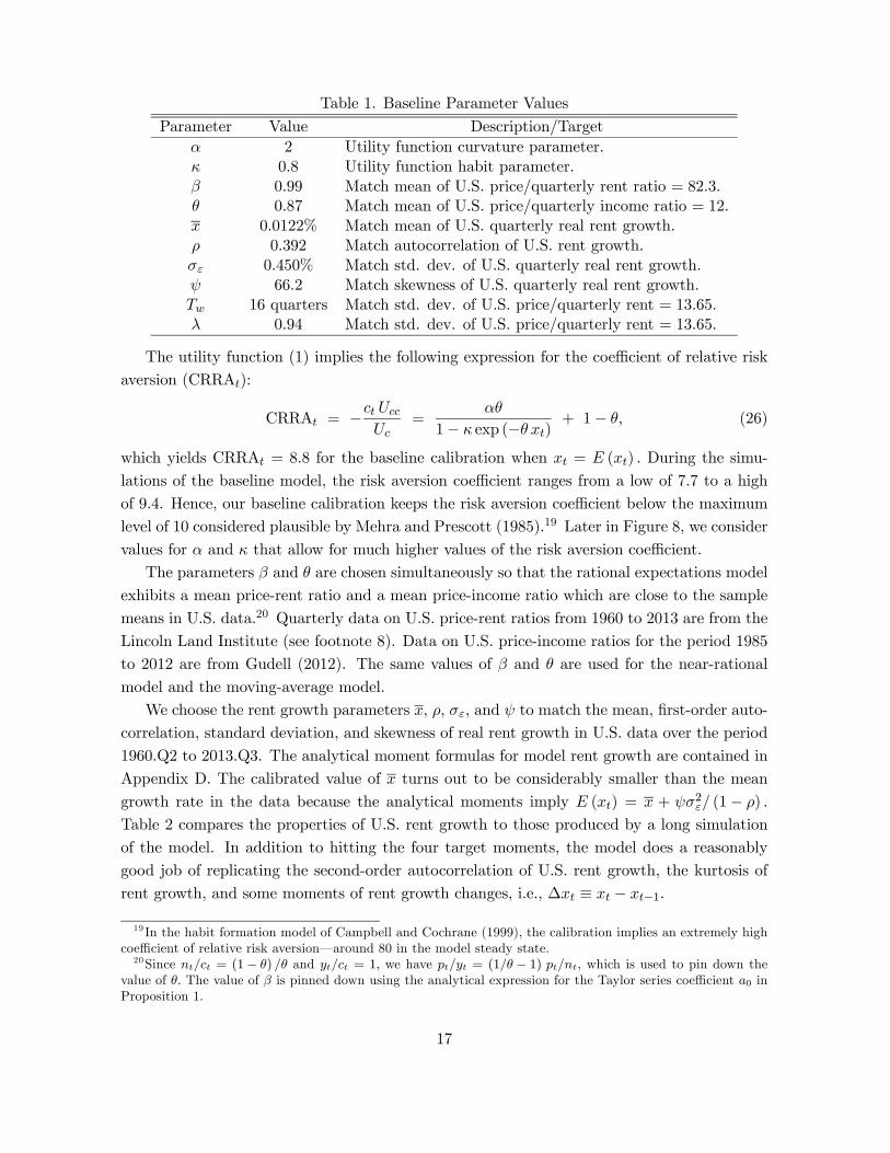
Table 1. Baseline Parameter Values
Parameter Value Description/Target
2 Utility function curvature parameter.
08 Utility function habit parameter.
099 Match mean of U.S. price/quarterly rent ratio = 823
087 Match mean of U.S. price/quarterly income ratio = 12
00122% Match mean of U.S. quarterly real rent growth.
0392 Match autocorrelation of U.S. rent growth.
0450% Match std. dev. of U.S. quarterly real rent growth.
662 Match skewness of U.S. quarterly real rent growth.
16 quarters Match std. dev. of U.S. price/quarterly rent = 1365
094 Match std. dev. of U.S. price/quarterly rent = 1365
The utility function (1) implies the following expression for the coefficient of relative risk
aversion (CRRA):
CRRA = −
=
1− exp (− ) + 1− (26)
which yields CRRA = 8.8 for the baseline calibration when = () During the simu-
lations of the baseline model, the risk aversion coefficient ranges from a low of 7.7 to a high
of 9.4. Hence, our baseline calibration keeps the risk aversion coefficient below the maximum
level of 10 considered plausible by Mehra and Prescott (1985).19 Later in Figure 8, we consider
values for and that allow for much higher values of the risk aversion coefficient.
The parameters and are chosen simultaneously so that the rational expectations model
exhibits a mean price-rent ratio and a mean price-income ratio which are close to the sample
means in U.S. data.20 Quarterly data on U.S. price-rent ratios from 1960 to 2013 are from the
Lincoln Land Institute (see footnote 8). Data on U.S. price-income ratios for the period 1985
to 2012 are from Gudell (2012). The same values of and are used for the near-rational
model and the moving-average model.
We choose the rent growth parameters and to match the mean, first-order auto-
correlation, standard deviation, and skewness of real rent growth in U.S. data over the period
1960.Q2 to 2013.Q3. The analytical moment formulas for model rent growth are contained in
Appendix D. The calibrated value of turns out to be considerably smaller than the mean
growth rate in the data because the analytical moments imply () = + 2 (1− )
Table 2 compares the properties of U.S. rent growth to those produced by a long simulation
of the model. In addition to hitting the four target moments, the model does a reasonably
good job of replicating the second-order autocorrelation of U.S. rent growth, the kurtosis of
rent growth, and some moments of rent growth changes, i.e., ∆ ≡ − −1
19 In the habit formation model of Campbell and Cochrane (1999), the calibration implies an extremely high
coefficient of relative risk aversion–around 80 in the model steady state.20Since = (1− ) and = 1 we have = (1 − 1) , which is used to pin down the
value of The value of is pinned down using the analytical expression for the Taylor series coefficient 0 in
Proposition 1.
17
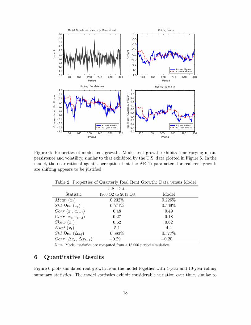
Figure 6: Properties of model rent growth. Model rent growth exhibits time-varying mean,
persistence and volatility, similar to that exhibited by the U.S. data plotted in Figure 5. In the
model, the near-rational agent’s perception that the AR(1) parameters for real rent growth
are shifting appears to be justified.
Table 2. Properties of Quarterly Real Rent Growth: Data versus Model
Statistic
U.S. Data
1960.Q2 to 2013.Q3 Model
() 0232% 0226%
() 0571% 0569%
( −1) 048 049
( −2) 027 018
() 062 062
() 51 44
(∆) 0583% 0577%
(∆ ∆−1) −029 −020Note: Model statistics are computed from a 15,000 period simulation.
6 Quantitative Results
Figure 6 plots simulated rent growth from the model together with 4-year and 10-year rolling
summary statistics. The model statistics exhibit considerable variation over time, similar to
18
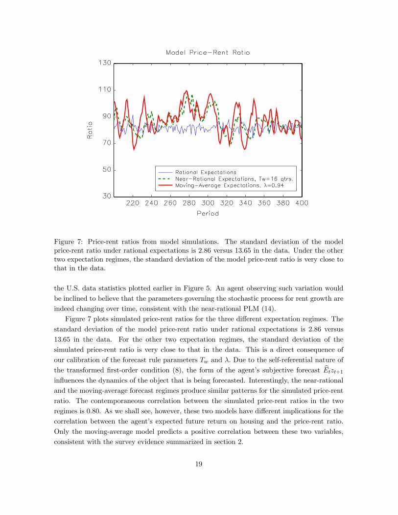
Figure 7: Price-rent ratios from model simulations. The standard deviation of the model
price-rent ratio under rational expectations is 2.86 versus 13.65 in the data. Under the other
two expectation regimes, the standard deviation of the model price-rent ratio is very close to
that in the data.
the U.S. data statistics plotted earlier in Figure 5. An agent observing such variation would
be inclined to believe that the parameters governing the stochastic process for rent growth are
indeed changing over time, consistent with the near-rational PLM (14).
Figure 7 plots simulated price-rent ratios for the three different expectation regimes. The
standard deviation of the model price-rent ratio under rational expectations is 2.86 versus
13.65 in the data. For the other two expectation regimes, the standard deviation of the
simulated price-rent ratio is very close to that in the data. This is a direct consequence of
our calibration of the forecast rule parameters and Due to the self-referential nature of
the transformed first-order condition (8), the form of the agent’s subjective forecast b+1
influences the dynamics of the object that is being forecasted. Interestingly, the near-rational
and the moving-average forecast regimes produce similar patterns for the simulated price-rent
ratio. The contemporaneous correlation between the simulated price-rent ratios in the two
regimes is 0.80. As we shall see, however, these two models have different implications for the
correlation between the agent’s expected future return on housing and the price-rent ratio.
Only the moving-average model predicts a positive correlation between these two variables,
consistent with the survey evidence summarized in section 2.
19
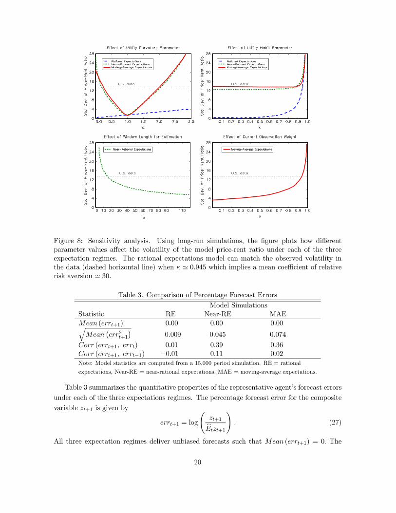
Figure 8: Sensitivity analysis. Using long-run simulations, the figure plots how different
parameter values affect the volatility of the model price-rent ratio under each of the three
expectation regimes. The rational expectations model can match the observed volatility in
the data (dashed horizontal line) when ' 0945 which implies a mean coefficient of relativerisk aversion ' 30.
Table 3. Comparison of Percentage Forecast Errors
Model Simulations
Statistic RE Near-RE MAE
(+1) 0.00 0.00 0.00q
¡2+1
¢0.009 0.045 0.074
(+1 ) 0.01 0.39 0.36
(+1 −1) −0.01 0.11 0.02
Note: Model statistics are computed from a 15,000 period simulation. RE = rational
expectations, Near-RE = near-rational expectations, MAE = moving-average expectations.
Table 3 summarizes the quantitative properties of the representative agent’s forecast errors
under each of the three expectations regimes. The percentage forecast error for the composite
variable +1 is given by
+1 = log
Ã+1b+1
! (27)
All three expectation regimes deliver unbiased forecasts such that (+1) = 0 The
20
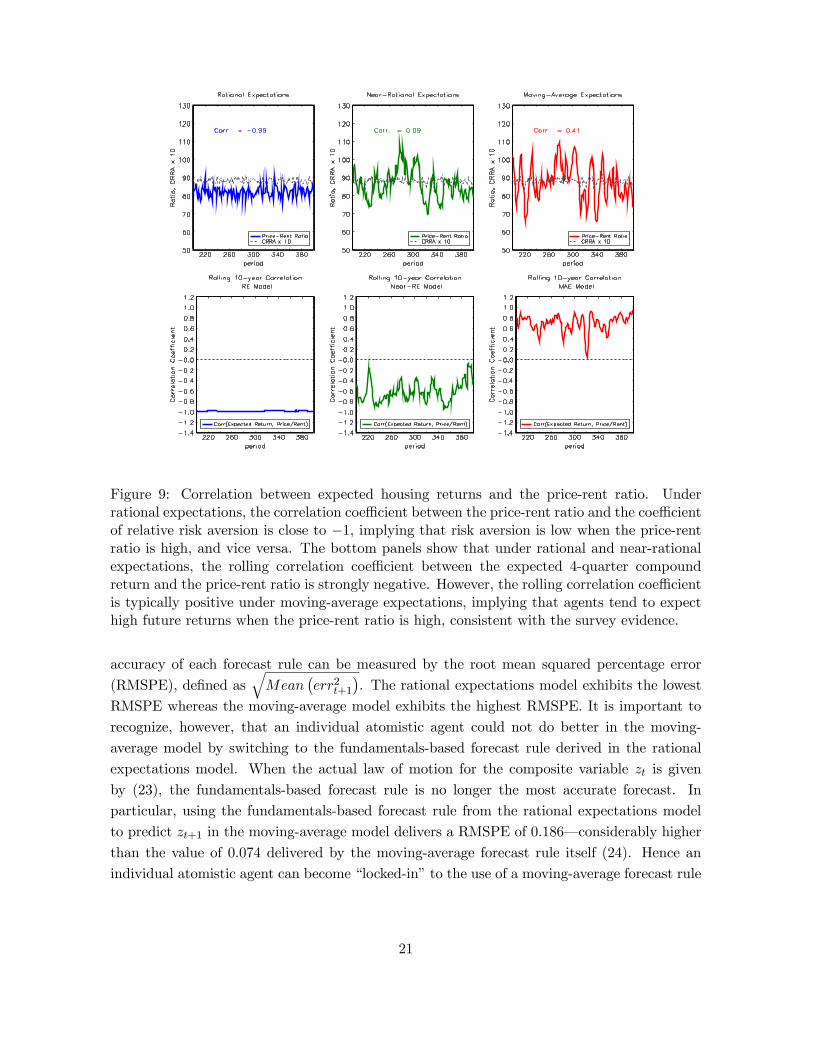
Figure 9: Correlation between expected housing returns and the price-rent ratio. Under
rational expectations, the correlation coefficient between the price-rent ratio and the coefficient
of relative risk aversion is close to −1, implying that risk aversion is low when the price-rentratio is high, and vice versa. The bottom panels show that under rational and near-rational
expectations, the rolling correlation coefficient between the expected 4-quarter compound
return and the price-rent ratio is strongly negative. However, the rolling correlation coefficient
is typically positive under moving-average expectations, implying that agents tend to expect
high future returns when the price-rent ratio is high, consistent with the survey evidence.
accuracy of each forecast rule can be measured by the root mean squared percentage error
(RMSPE), defined asq
¡2+1
¢. The rational expectations model exhibits the lowest
RMSPE whereas the moving-average model exhibits the highest RMSPE. It is important to
recognize, however, that an individual atomistic agent could not do better in the moving-
average model by switching to the fundamentals-based forecast rule derived in the rational
expectations model. When the actual law of motion for the composite variable is given
by (23), the fundamentals-based forecast rule is no longer the most accurate forecast. In
particular, using the fundamentals-based forecast rule from the rational expectations model
to predict +1 in the moving-average model delivers a RMSPE of 0.186–considerably higher
than the value of 0.074 delivered by the moving-average forecast rule itself (24). Hence an
individual atomistic agent can become “locked-in” to the use of a moving-average forecast rule
21
so long as other agents in the economy are using the same forecasting approach.21
Table 3 also shows that the autocorrelation of the forecast errors in both the near-rational
model and moving-average model are reasonably low–less than 0.4. Hence, a large amount of
data would be required for the representative agent in either model to reject the null hypothesis
of uncorrelated forecast errors, making it difficult for the agent to detect a misspecification of
the subjective forecast rule.
Figure 8 shows how some key parameter values affect the volatility of the model price-rent
ratio under each expectation regime. The dashed horizontal line in each panel marks the
observed standard deviation of 13.65 in U.S. data. In the top left panel, we examine the effect
of varying the utility curvature parameter over the range 0 ≤ ≤ 3 while holding and atthe baseline values shown in Table 1. From equation (26) with = () we have CRRA
= 0.13 when = 0 and CRRA = 13.1 when = 3. In the top right panel, we examine the
effect of varying the habit formation parameter over the range 0 ≤ ≤ 0975 while holding and at the baseline values shown in Table 1. In this case, the implied value of CRRA
with = () ranges from a low of 19 to a high of 64 The top right panel shows that the
rational expectations model can match the observed volatility in the data when ' 0945
which together with the baseline values of = 087 and = 2 delivers CRRA ' 30 when
= ()
The bottom two panels of Figure 8 show that lower values of (near-rational model)
or higher values of (moving-average model) both serve to magnify the volatility of the
simulated price-rent ratio. By construction, the baseline calibrated values of = 16 quarters
and = 094 deliver price-rent ratio volatilities that are close to those in the data.
Table 4 compares unconditional moments from the model to the corresponding moments
in U.S. data. The near-rational model and the moving-average model are both successful
in matching the volatility and persistence of the U.S. price-rent ratio. However, only the
moving-average model comes close to matching the strong persistence of U.S. housing returns,
delivering an autocorrelation coefficient for returns of 0.63 versus 0.59 in the data. Unfortu-
nately, none of the three expectation regimes can reproduce the strong negative skewness and
the large excess kurtosis of U.S. housing returns. The consideration of additional nonlineari-
ties, such as endogenous shifts between forecast rules, along the lines of Brock and Hommes
(1998), might allow the model to better match the higher return moments in the data.
21Lansing (2006) investigates the concept of forecast lock-in using a standard Lucas-type asset pricing model.
22
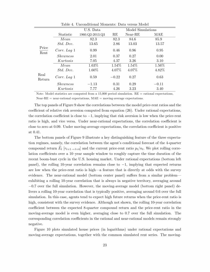
Table 4. Unconditional Moments: Data versus Model
U.S. Data Model Simulations
Statistic 1960.Q2-2013.Q3 RE Near-RE MAE
82.3 82.3 84.6 85.9
13.65 2.86 13.03 13.57Price
Rent 1 0.99 0.46 0.96 0.95
2.01 0.37 0.27 000
7.05 4.37 3.26 3.10
1.63% 1.54% 1.54% 1.56%
1.60% 4.07% 4.07% 4.82%
Real
Return 1 0.59 −022 0.27 0.63
−113 0.31 0.29 −011 7.77 4.26 3.23 3.40
Note: Model statistics are computed from a 15,000 period simulation. RE = rational expectations,
Near-RE = near-rational expectations, MAE = moving-average expectations.
The top panels of Figure 9 show the correlations between the model price-rent ratios and the
coefficient of relative risk aversion computed from equation (26). Under rational expectations,
the correlation coefficient is close to −1, implying that risk aversion is low when the price-rentratio is high, and vice versa. Under near-rational expectations, the correlation coefficient is
close to zero at 0.09. Under moving-average expectations, the correlation coefficient is positive
at 0.41.
The bottom panels of Figure 9 illustrate a key distinguishing feature of the three expecta-
tion regimes, namely, the correlation between the agent’s conditional forecast of the 4-quarter
compound return b [+1→ +4] and the current price-rent ratio We plot rolling corre-
lation coefficients over a 10—year sample window to roughly capture the time duration of the
recent boom-bust cycle in the U.S. housing market. Under rational expectations (bottom left
panel), the rolling 10-year correlation remains close to −1, implying that expected returnsare low when the price-rent ratio is high–a feature that is directly at odds with the survey
evidence. The near-rational model (bottom center panel) suffers from a similar problem–
exhibiting a rolling 10-year correlation that is always in negative territory, averaging around
−07 over the full simulation. However, the moving-average model (bottom right panel) de-
livers a rolling 10-year correlation that is typically positive, averaging around 06 over the full
simulation. In this case, agents tend to expect high future returns when the price-rent ratio is
high, consistent with the survey evidence. Although not shown, the rolling 10-year correlation
coefficient between the expected 8-quarter compound return and the price-rent ratio in the
moving-average model is even higher, averaging close to 07 over the full simulation. The
corresponding correlation coefficients in the rational and near-rational models remain strongly
negative.
Figure 10 plots simulated house prices (in logarithms) under rational expectations and
moving-average expectations, together with the common simulated rent series. The moving-
23
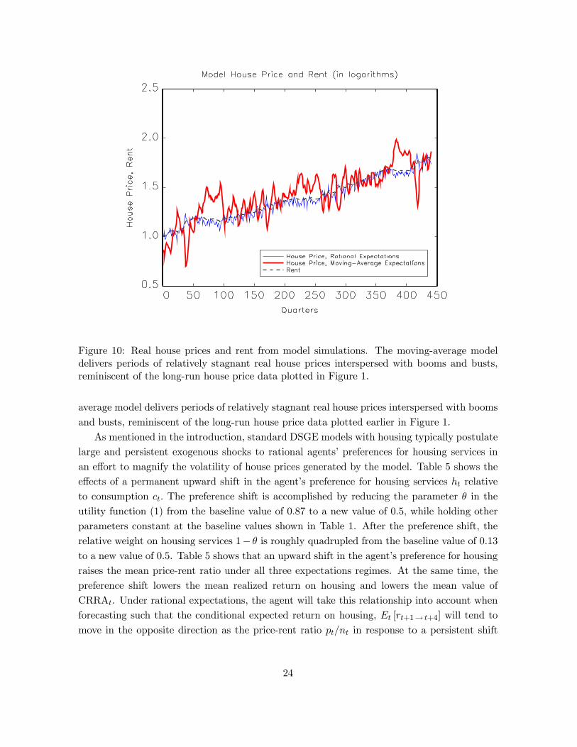
Figure 10: Real house prices and rent from model simulations. The moving-average model
delivers periods of relatively stagnant real house prices interspersed with booms and busts,
reminiscent of the long-run house price data plotted in Figure 1.
average model delivers periods of relatively stagnant real house prices interspersed with booms
and busts, reminiscent of the long-run house price data plotted earlier in Figure 1.
As mentioned in the introduction, standard DSGE models with housing typically postulate
large and persistent exogenous shocks to rational agents’ preferences for housing services in
an effort to magnify the volatility of house prices generated by the model. Table 5 shows the
effects of a permanent upward shift in the agent’s preference for housing services relative
to consumption The preference shift is accomplished by reducing the parameter in the
utility function (1) from the baseline value of 0.87 to a new value of 0.5, while holding other
parameters constant at the baseline values shown in Table 1. After the preference shift, the
relative weight on housing services 1− is roughly quadrupled from the baseline value of 0.13
to a new value of 0.5. Table 5 shows that an upward shift in the agent’s preference for housing
raises the mean price-rent ratio under all three expectations regimes. At the same time, the
preference shift lowers the mean realized return on housing and lowers the mean value of
CRRA. Under rational expectations, the agent will take this relationship into account when
forecasting such that the conditional expected return on housing, [+1→ +4] will tend to
move in the opposite direction as the price-rent ratio in response to a persistent shift
24
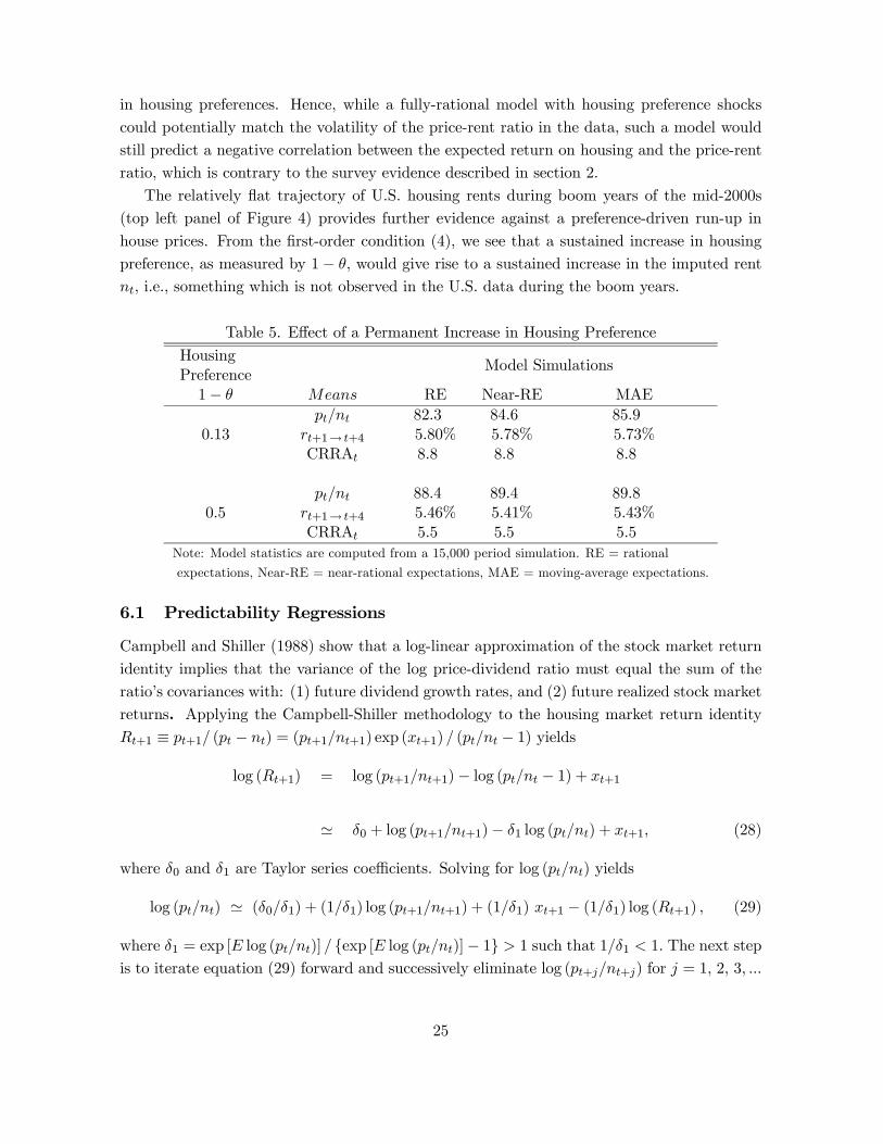
in housing preferences. Hence, while a fully-rational model with housing preference shocks
could potentially match the volatility of the price-rent ratio in the data, such a model would
still predict a negative correlation between the expected return on housing and the price-rent
ratio, which is contrary to the survey evidence described in section 2.
The relatively flat trajectory of U.S. housing rents during boom years of the mid-2000s
(top left panel of Figure 4) provides further evidence against a preference-driven run-up in
house prices. From the first-order condition (4), we see that a sustained increase in housing
preference, as measured by 1− would give rise to a sustained increase in the imputed rent
i.e., something which is not observed in the U.S. data during the boom years.
Table 5. Effect of a Permanent Increase in Housing Preference
Housing
PreferenceModel Simulations
1− RE Near-RE MAE
0.13
+1→ +4
CRRA
82.3
5.80%
8.8
84.6
5.78%
8.8
85.9
5.73%
8.8
0.5
+1→ +4
CRRA
88.4
5.46%
5.5
89.4
5.41%
5.5
89.8
5.43%
5.5
Note: Model statistics are computed from a 15,000 period simulation. RE = rational
expectations, Near-RE = near-rational expectations, MAE = moving-average expectations.
6.1 Predictability Regressions
Campbell and Shiller (1988) show that a log-linear approximation of the stock market return
identity implies that the variance of the log price-dividend ratio must equal the sum of the
ratio’s covariances with: (1) future dividend growth rates, and (2) future realized stock market
returns. Applying the Campbell-Shiller methodology to the housing market return identity
+1 ≡ +1 ( − ) = (+1+1) exp (+1) ( − 1) yields
log (+1) = log (+1+1)− log ( − 1) + +1
' 0 + log (+1+1)− 1 log () + +1 (28)
where 0 and 1 are Taylor series coefficients. Solving for log () yields
log () ' (01) + (11) log (+1+1) + (11) +1 − (11) log (+1) (29)
where 1 = exp [ log ()] {exp [ log ()]− 1} 1 such that 11 1 The next stepis to iterate equation (29) forward and successively eliminate log (++) for = 1 2 3
25
Applying a transversality condition such that lim→∞ (11) log (++) = 0 yields
log () ' 0
1 − 1 +∞P=1
(11) [+ − log (+)] (30)
which shows that movements in the log price-rent ratio must be accounted for by movements
in either future rent growth rates or future log housing returns (both measured in real terms).
The variables in the approximate return identity (30) can be expressed as deviations from
their unconditional means, while the means are consolidated into the constant term. Multi-
plying both sides of the resulting expression by log ()− log () and then taking the
unconditional expectation of both sides yields
() =
"log ()
∞P=1
(11) +
#
−
"log ()
∞P=1
(11) log(+)
# (31)
Equation (31) states that the variance of the log price-rent ratio must be accounted for
by the covariance of the log price-rent ratio with either: (1) future rent growth rates, or (2)
future realized housing returns. The magnitude of each covariance term is a measure of the
predictability of future rent growth or future realized returns when the current price-rent ratio
is employed as the sole regressor in a forecasting equation.
To investigate the predictability implications of our model versus those in the data, we
estimate the following regression equations:
+1→ +4 ≡4P
=1
log (+) = constant + b log () + +1 (32)
+1→ +4 ≡4P
=1
+ = constant + b log () + +1 (33)
where +1 and +1 are statistical error terms.
Table 6 reports the results of predictability regressions in the form of equations (32) or (33).
In the case of the U.S. stock market, it is well documented that the log price-dividend ratio
exhibits strong predictive power for future realized stock returns but weak predictive power
for future dividend growth rates (Cochrane 2008, Engsted, et al. 2012). Table 6 shows that
analogous results are obtained for the U.S. housing market, particularly in the more recent
sample period starting in the year 2000. The 2 statistic is much larger in the regression that
seeks to predict future returns versus the regression that seeks to predict future rent growth.
In the return regression (top panel of Table 6), the estimated coefficient b is consistently largeand negative, implying that a higher price-rent ratio predicts lower realized returns in the
future. In the rent growth regression (bottom panel of Table 6), b is negative and significantover the full sample starting in 1960, but insignificant and very close to zero in the more recent
sample starting in the year 2000.
26
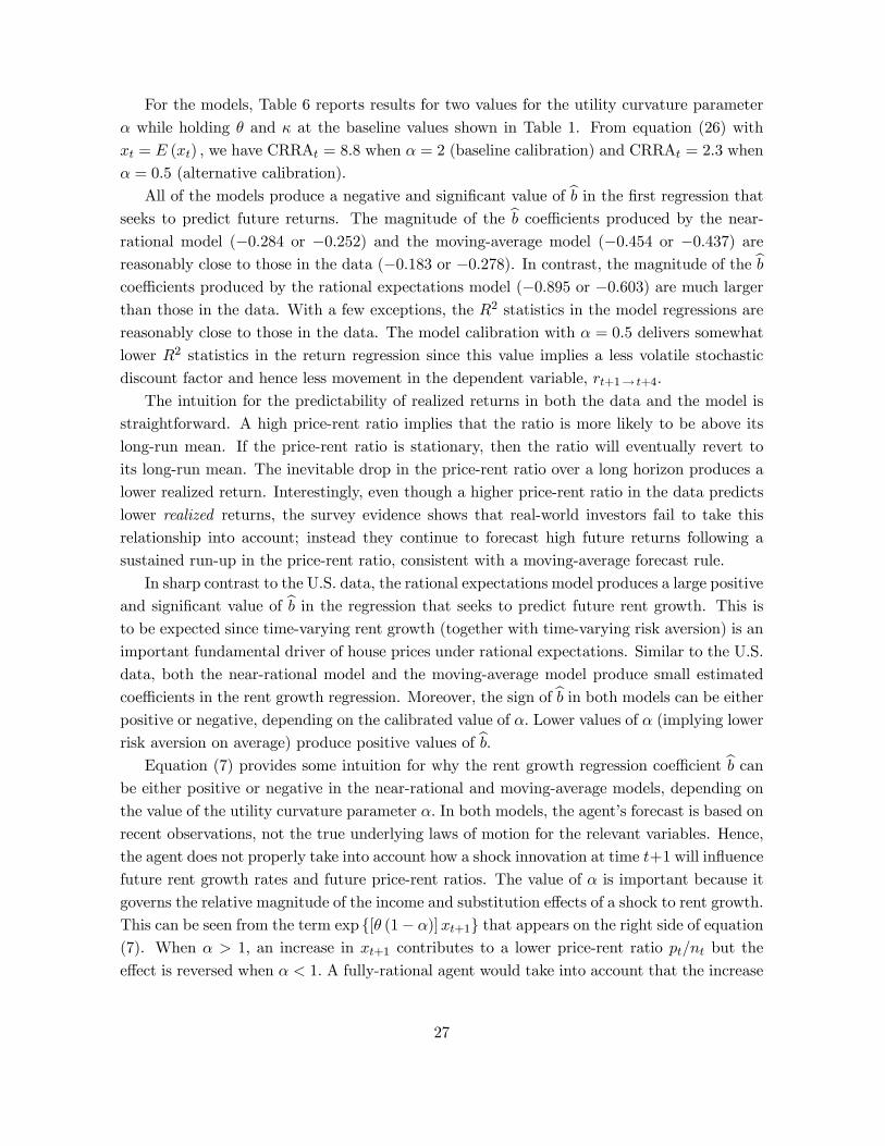
For the models, Table 6 reports results for two values for the utility curvature parameter
while holding and at the baseline values shown in Table 1. From equation (26) with
= () we have CRRA = 8.8 when = 2 (baseline calibration) and CRRA = 2.3 when
= 05 (alternative calibration).
All of the models produce a negative and significant value of b in the first regression thatseeks to predict future returns. The magnitude of the b coefficients produced by the near-rational model (−0284 or −0252) and the moving-average model (−0454 or −0437) arereasonably close to those in the data (−0183 or −0278). In contrast, the magnitude of the bcoefficients produced by the rational expectations model (−0895 or −0603) are much largerthan those in the data. With a few exceptions, the 2 statistics in the model regressions are
reasonably close to those in the data. The model calibration with = 05 delivers somewhat
lower 2 statistics in the return regression since this value implies a less volatile stochastic
discount factor and hence less movement in the dependent variable, +1→ +4
The intuition for the predictability of realized returns in both the data and the model is
straightforward. A high price-rent ratio implies that the ratio is more likely to be above its
long-run mean. If the price-rent ratio is stationary, then the ratio will eventually revert to
its long-run mean. The inevitable drop in the price-rent ratio over a long horizon produces a
lower realized return. Interestingly, even though a higher price-rent ratio in the data predicts
lower realized returns, the survey evidence shows that real-world investors fail to take this
relationship into account; instead they continue to forecast high future returns following a
sustained run-up in the price-rent ratio, consistent with a moving-average forecast rule.
In sharp contrast to the U.S. data, the rational expectations model produces a large positive
and significant value of b in the regression that seeks to predict future rent growth. This isto be expected since time-varying rent growth (together with time-varying risk aversion) is an
important fundamental driver of house prices under rational expectations. Similar to the U.S.
data, both the near-rational model and the moving-average model produce small estimated
coefficients in the rent growth regression. Moreover, the sign of b in both models can be eitherpositive or negative, depending on the calibrated value of Lower values of (implying lower
risk aversion on average) produce positive values of b.Equation (7) provides some intuition for why the rent growth regression coefficient b can
be either positive or negative in the near-rational and moving-average models, depending on
the value of the utility curvature parameter In both models, the agent’s forecast is based on
recent observations, not the true underlying laws of motion for the relevant variables. Hence,
the agent does not properly take into account how a shock innovation at time +1 will influence
future rent growth rates and future price-rent ratios. The value of is important because it
governs the relative magnitude of the income and substitution effects of a shock to rent growth.
This can be seen from the term exp {[ (1− )]+1} that appears on the right side of equation(7). When 1 an increase in +1 contributes to a lower price-rent ratio but the
effect is reversed when 1 A fully-rational agent would take into account that the increase
27
in +1 also serves to increase +1+1 but that forecast channel is distorted in the near-
rational and moving-average models. Consequently, the term involving exp {[ (1− )]+1}tends to dominate the sign of the rent growth regression coefficient in these two models. In
contrast, the return regression coefficient exhibits a consistent negative sign across all models,
regardless of the value of because the sign of the coefficient is driven by the mean-reverting
properties of the price-rent ratio.
In a recent study using price and rent data from the housing markets of 18 OECD countries
over the period 1970 to 2011, Engsted and Pedersen (2012) find evidence of cross-country and
sub-sample instability in the estimated coefficients for predictive regressions that take the form
of equations (32) or (33). Using data either before or after 1995, they find that the estimated
regression coefficients for a given country can be either positive or negative when predicting
future rent growth along the lines of equation (33). Table 6 confirms a similar sort of instability
in the sign of b when attempting to predict future U.S. rent growth using either the full sampleof data from 1960 to 2011 or the more recent sample from 2000 to 2011. Engsted and Pedersen
(2012) also find that the relative magnitude of the 2 statistics for the two types of predictive
regressions can differ across countries and across time periods for a given country. In line with
their overall empirical findings, our simulation results show that, depending on the nature of
the expectation regime and the degree of curvature in the agent’s utility function, the signs
and magnitudes of the estimated regression coefficients and the resulting 2 statistics can vary
substantially, particularly with respect to rent growth predictability.
Table 6. Predictability Regressions: Data versus Model
Model Simulations
U.S. Data RE Near-RE MAEb b b bPredictive
Regression
1960.Q2-
2013.Q3
2000.Q1-
2013.Q3 = 2 = 05 = 2 = 05 = 2 = 05
+1→ +4−0183(0024)
−0278(0077)
−0895 −0603(0011) (0017)
−0284 −0252(0005) (0006)
−0453 −0437(0006) (0008)
2 (%) 21.4 21.3 317 78 197 92 301 170
+1→ +4−0039(0007)
−0001(0014)
0111 0398
(0004) (0011)
−0002 0021
(0001) (0002)
−0008 0026
(0001) (0001)
2 (%) 11.9 0.0 58 85 00 12 08 23
Notes: Standard errors in parenthesis. Model regressions use data from a 15,000 period simulation. RE =
rational expectations, Near-RE =near-rational expectations, MAE = moving-average expectations. Returns
and rent growth in U.S. data are measured in real terms.
28
7 Conclusion
Stories involving speculative bubbles can be found throughout history in various countries and
asset markets. These episodes can have important consequences for the economy as firms and
investors respond to the price signals, potentially resulting in capital misallocation.22 The
typical transitory nature of these run-ups should perhaps be viewed as a long-run victory
for fundamental asset pricing theory. Still, it remains a challenge for fundamental theory to
explain the ever-present volatility of asset prices within a framework of efficient markets and
fully-rational agents.
Like stock prices, real-world house prices exhibit periods of stagnation interspersed with
boom-bust cycles. A reasonably-parameterized rational expectations model significantly un-
derpredicts the volatility of the U.S. price-rent ratio, even when allowing for time-varying risk
aversion and time-varying stochastic properties of rent growth. We showed that a standard
asset pricing model can match the volatility and persistence of the U.S. price-rent ratio, as
well as other quantitative and qualitative features of the data, if agents in the model employ
simple moving-average forecast rules. With such a forecast rule, agents tend to expect higher
future returns when house prices are high relative to fundamentals–a feature that is consistent
with survey evidence on the expectations of real-world housing investors. The moving average
model is also successful in generating data that is broadly consistent with the predictabil-
ity properties of future realized housing returns and future rent growth that are observed in
housing market data for the U.S. and other countries.
22Lansing (2012) examines the welfare consequences of speculative bubbles in a model where excessive asset
price movements can affect the economy’s trend growth rate.
29
A Appendix: Effect of a Borrowing Constraint
Here we show analytically how imputed rent can reflect not only a utility dividend, but also the
marginal collateral value of the house in the case when the representative agent’s borrowing
constraint is binding. Following Campbell and Hercowitz (2009), the representative agent’s
problem in the presence of a borrowing constraint can be formulated as
max +1
b0 ∞X=0
£ (A.1)
where the current-period Lagrangian £ is given by
£ =
³
1− −
−11−−1´1−
− 11−
+ [ + +1 + (−1 − )− −]
+ [ − +1] (A.2)
In the above expression, +1 is the stock of mortgage debt at the end of period and is the
gross real interest rate on the debt. The last term of the Lagrangian reflects the borrowing
constraint which says that the agent may only borrow up to a fraction ≥ 0 of the currenthousing value . When the Lagrange multiplier 0 the borrowing constraint is binding.
From (A.2), the first-order conditions with respect to and +1 are given by
=
µ1−
¶ + | {z }≡
+ b+1
| {z }≡ +1
+1 (A.3)
= 1 − +1 (A.4)
where we have divided both sides by and imposed the equilibrium condition = 1 Com-
paring equation (A.3) to the original first-order condition (4) shows that the imputed rent
now consists of two terms: the standard utility dividend plus the marginal collateral value
of the house in the case when the borrowing constraint is binding, i.e., when 0 Hence,
by calibrating the effective cash flows in the model to mimic the stochastic properties of rent
growth in the data, we implicitly (but imperfectly) take into account the effect of a binding
borrowing constraint on the equilibrium house price.
B Appendix: Approximate Rational Solution
The methodology for computing the rational expectations solution in Proposition 1 follows
the procedure in Lansing (2010). First we rewrite the law of motion for rent growth (5) as
30
follows
+1 − () = [ − ()] + (1− ) [− ()]| {z }=−21−
++1 + ( − )| {z }≡
= [ − ()] + +1 + ¡ − 2
¢ (B.1)
where is the deterministic steady state growth rate, () is the ergodic mean growth rate,
and we have made use of [ ( − )] = () = 2
The law of motion for +1 − 2 follows directly from the law of motion for rent growth
(5) and the rewritten version (B.1):
+1 − 2 = +1 (+1 − )− 2
= +1 [+1 − ()] + +1 [ ()− ]| {z }=21−
−2
= +1
½ [ − ()] +
¡ − 2
¢+
21−
¾+¡2+1 − 2
¢ (B.2)
Iterating ahead the conjectured law of motion for yields
+1 = 0 exp©1 [+1 − ()] + 2
¡+1 − 2
¢ª (B.3)
Substituting equations (B.1) and (B.2) into equation (B.3) and then taking the conditional
expectation yields
+1 = 0 expn1 [ − ()] + 1
¡ − 2
¢+ (2)
2 4 +122
2
o (B.4)
where ≡ 1 + 2 [ − ()] + 2¡ − 2
¢+ 2
21−
In deriving (B.4), we have used the properties of the conditional lognormal distribution which
imply
exp¡2
2+1
¢= exp
©
¡2
2+1
¢+ 12
¡2
2+1
¢ª
= expn
¡2
2+1
¢+ 12
h¡2
2+1
¢2i− 12
£
¡2
2+1
¢¤2o
= expn2
2 +
12(2)
2 34 − 12(2)
2 4
o
= exph2
2 + (2)
2 4
i (B.5)
31
Next, we substitute the conditional expectation (B.4) into the transformed first-order con-
dition (8) and then take logarithms to obtain
log () = ( ) = log { () +
0 exph (1− ) + 1 [ − ()] + 1
¡ − 2
¢+ (2)
2 4 +122
2
io
' log (0) + 1 [ − ()] + 2¡ − 2
¢ (B.6)
The expressions for the Taylor-series coefficients 0 = exp [ log ()] 1 and 2 are derived
as follows
log (0) = [ () ()] (B.7)
1 =
¯̄̄̄() ()
(B.8)
2 =
¯̄̄̄() ()
(B.9)
where () = +2 (1− ) and () = 2 Solving the above three equations yields the
values for the three undetermined coefficients.
Taking logs of equation (B.3) and then forming the conditional expectation yields
log (+1) = log (0) + 1 [+1 − ()] + 2
¡+1 − 2
¢
= log (0) + 1 [ − ()] + 1¡ − 2
¢ (B.10)
where
¡+1 − 2
¢= 0 from equation (B.2). The above expression and equation (B.4) are
used to compute the expected log return in equation (12).
C Appendix: Approximate Near-Rational Solution
First we solve for the perceived rational solution in the case when the perceived AR(1) pa-
rameters for rent growth are constant such that = = and = for all The
near-rational agent’s conjectured law of motion in this case is given by
' 0 exp [ 1 ( − )] (C.1)
Iterating ahead the conjectured law of motion for and taking the subjective conditional
expectation yields b+1 = 0 exph1 ( − ) + 1
2(1)
2 2
i (C.2)
32
Substituting the conditional forecast (C.2) into the transformed first-order condition (8) and
then taking logarithms yields
log () = () = logn () + 0 exp
h (1− ) + 1 ( − ) + 1
2(1)
2 2
io' log (0) + 1 ( − ) (C.3)
where 0 ≡ exp [ log ()] and 1 are Taylor-series coefficients. The expressions for the Taylor
series coefficients are are derived as follows
log (0) = () = logn () + 0 exp
h (1− )+ 1
2(1)
2 2
io (C.4)
1 = 0 () =1
0
n 0 () + 0 [ (1− ) + 1] exp
h (1− )+ 1
2(1)
2 2
io
(C.5)
which yield a set of two equations that can be solved for the two undetermined coefficients 0
and 1
For the case when the perceived AR(1) parameters are shifting as in the near-rational PLM
(14), equations (C.4) and (C.5) can be rewritten as
0 = ()
1− exph (1− ) +
12(1)
2 2
i (C.6)
1 = 0 ()0
+ [ (1− ) + 1 ] exph (1− ) +
12(1)
2 2
i (C.7)
where we have substituted in the most recent estimates for the perceived AR(1) parameters, as
given by and We follow the common practice in the learning literature by assuming
that the agent views the most recent parameter estimates as permanent when computing
the subjective forecast b +1 Given the most recent estimates for the AR(1) parameters,
equations (C.6) and (C.7) are solved simultaneously each period to obtain values for 0 and
1 for use in the subjective forecast (19). The subjective forecast is substituted into the
transformed first-order condition (8) to obtain the actual law of motion (20).
Iterating ahead the perceived law of motion (18) and then taking logs and forming the
subjective conditional expectation yieldsb log (+1) = b [log (0+1) + 1+1 (+1 − +1)]
= log (0) + 1 ( − ) (C.8)
where once again we assume that the agent views the most recent parameter estimates and
as permanent such that the most recent values for 0 and 1 are also viewed as permanent.
The above expression and b +1 from equation (19) are used to compute the expected log
return in equation (21).
33
D Appendix: Moments of Rent Growth
This section summarizes the formulas for the unconditional moments of rent growth which are
used to calibrate the true law of motion (5). From Granger and Andersen (1978) and Sesay
and Subba Rao (1988), we have
( − ) ≡1 =21−
(D.1)
h( − )2
i≡2 =
2£1 + 222 + 41
¤1− 2 − 22
(D.2)
[( − ) (−1 − )] ≡11 = 2 + 221 (D.3)
h( − )3
i≡3 =
2£634 + 3
¡1 + 622
¢1 + 9
¡2 + 22
¢2
¤1− 3 − 322
(D.4)
h( − )4
i≡4 =
2{32(844−1)+96341+6[1+1222(2+22)]2+16(2+322)3}1−4−6222−344
(D.5)
Given the above expressions, the moments of can be computed as follows
() = +1 (D.6)
() = 2 − (1)2 (D.7)
( −1) =11 − (1)
2
() (D.8)
() =3 − (1)
3 − 31 ()
()15
(D.9)
() =4 + (1)
4 − 41
h3 + (1)
3i+ 62 (1)
2
()2
(D.10)
34
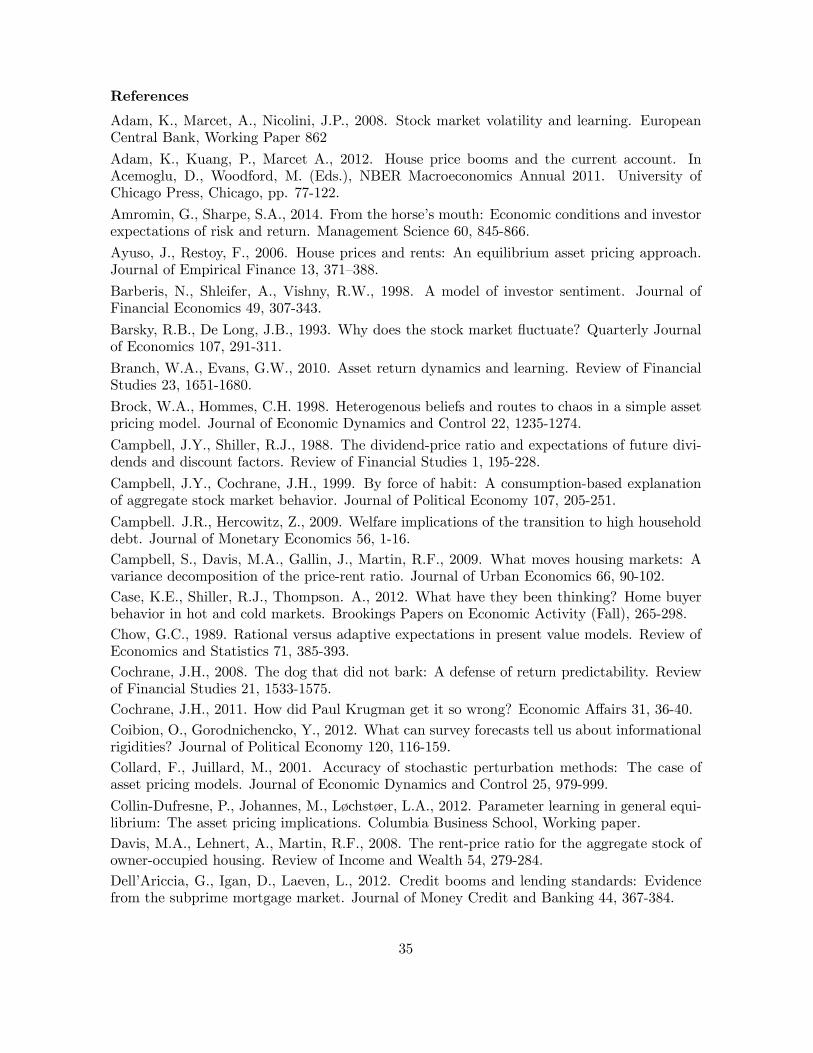
References
Adam, K., Marcet, A., Nicolini, J.P., 2008. Stock market volatility and learning. EuropeanCentral Bank, Working Paper 862
Adam, K., Kuang, P., Marcet A., 2012. House price booms and the current account. InAcemoglu, D., Woodford, M. (Eds.), NBER Macroeconomics Annual 2011. University ofChicago Press, Chicago, pp. 77-122.
Amromin, G., Sharpe, S.A., 2014. From the horse’s mouth: Economic conditions and investorexpectations of risk and return. Management Science 60, 845-866.
Ayuso, J., Restoy, F., 2006. House prices and rents: An equilibrium asset pricing approach.Journal of Empirical Finance 13, 371—388.
Barberis, N., Shleifer, A., Vishny, R.W., 1998. A model of investor sentiment. Journal ofFinancial Economics 49, 307-343.
Barsky, R.B., De Long, J.B., 1993. Why does the stock market fluctuate? Quarterly Journalof Economics 107, 291-311.
Branch, W.A., Evans, G.W., 2010. Asset return dynamics and learning. Review of FinancialStudies 23, 1651-1680.
Brock, W.A., Hommes, C.H. 1998. Heterogenous beliefs and routes to chaos in a simple assetpricing model. Journal of Economic Dynamics and Control 22, 1235-1274.
Campbell, J.Y., Shiller, R.J., 1988. The dividend-price ratio and expectations of future divi-dends and discount factors. Review of Financial Studies 1, 195-228.
Campbell, J.Y., Cochrane, J.H., 1999. By force of habit: A consumption-based explanationof aggregate stock market behavior. Journal of Political Economy 107, 205-251.
Campbell. J.R., Hercowitz, Z., 2009. Welfare implications of the transition to high householddebt. Journal of Monetary Economics 56, 1-16.
Campbell, S., Davis, M.A., Gallin, J., Martin, R.F., 2009. What moves housing markets: Avariance decomposition of the price-rent ratio. Journal of Urban Economics 66, 90-102.
Case, K.E., Shiller, R.J., Thompson. A., 2012. What have they been thinking? Home buyerbehavior in hot and cold markets. Brookings Papers on Economic Activity (Fall), 265-298.
Chow, G.C., 1989. Rational versus adaptive expectations in present value models. Review ofEconomics and Statistics 71, 385-393.
Cochrane, J.H., 2008. The dog that did not bark: A defense of return predictability. Reviewof Financial Studies 21, 1533-1575.
Cochrane, J.H., 2011. How did Paul Krugman get it so wrong? Economic Affairs 31, 36-40.
Coibion, O., Gorodnichencko, Y., 2012. What can survey forecasts tell us about informationalrigidities? Journal of Political Economy 120, 116-159.
Collard, F., Juillard, M., 2001. Accuracy of stochastic perturbation methods: The case ofasset pricing models. Journal of Economic Dynamics and Control 25, 979-999.
Collin-Dufresne, P., Johannes, M., Løchstøer, L.A., 2012. Parameter learning in general equi-librium: The asset pricing implications. Columbia Business School, Working paper.
Davis, M.A., Lehnert, A., Martin, R.F., 2008. The rent-price ratio for the aggregate stock ofowner-occupied housing. Review of Income and Wealth 54, 279-284.
Dell’Ariccia, G., Igan, D., Laeven, L., 2012. Credit booms and lending standards: Evidencefrom the subprime mortgage market. Journal of Money Credit and Banking 44, 367-384.
35
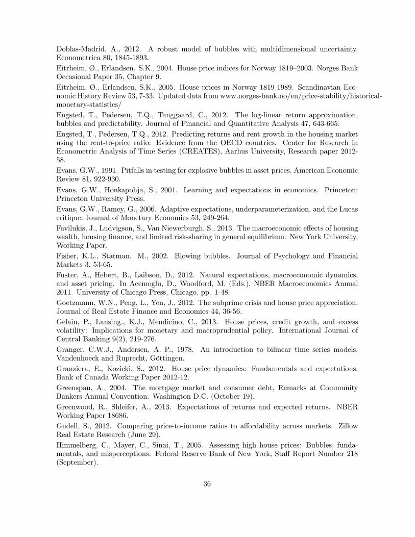
Doblas-Madrid, A., 2012. A robust model of bubbles with multidimensional uncertainty.Econometrica 80, 1845-1893.
Eitrheim, Ø., Erlandsen. S.K., 2004. House price indices for Norway 1819—2003. Norges BankOccasional Paper 35, Chapter 9.
Eitrheim, Ø., Erlandsen, S.K., 2005. House prices in Norway 1819-1989. Scandinavian Eco-nomic History Review 53, 7-33. Updated data from www.norges-bank.no/en/price-stability/historical-monetary-statistics/
Engsted, T., Pedersen, T.Q., Tanggaard, C., 2012. The log-linear return approximation,bubbles and predictability. Journal of Financial and Quantitative Analysis 47, 643-665.
Engsted, T., Pedersen, T.Q., 2012. Predicting returns and rent growth in the housing marketusing the rent-to-price ratio: Evidence from the OECD countries. Center for Research inEconometric Analysis of Time Series (CREATES), Aarhus University, Research paper 2012-58.
Evans, G.W., 1991. Pitfalls in testing for explosive bubbles in asset prices. American EconomicReview 81, 922-930.
Evans, G.W., Honkapohja, S., 2001. Learning and expectations in economics. Princeton:Princeton University Press.
Evans, G.W., Ramey, G., 2006. Adaptive expectations, underparameterization, and the Lucascritique. Journal of Monetary Economics 53, 249-264.
Favilukis, J., Ludvigson, S., Van Niewerburgh, S., 2013. The macroeconomic effects of housingwealth, housing finance, and limited risk-sharing in general equilibrium. New York University,Working Paper.
Fisher, K.L., Statman. M., 2002. Blowing bubbles. Journal of Psychology and FinancialMarkets 3, 53-65.
Fuster, A., Hebert, B., Laibson, D., 2012. Natural expectations, macroeconomic dynamics,and asset pricing. In Acemoglu, D., Woodford, M. (Eds.), NBER Macroeconomics Annual2011. University of Chicago Press, Chicago, pp. 1-48.
Goetzmann, W.N., Peng, L., Yen, J., 2012. The subprime crisis and house price appreciation.Journal of Real Estate Finance and Economics 44, 36-56.
Gelain, P., Lansing., K.J., Mendicino, C., 2013. House prices, credit growth, and excessvolatility: Implications for monetary and macroprudential policy. International Journal ofCentral Banking 9(2), 219-276.
Granger, C.W.J., Andersen, A. P., 1978. An introduction to bilinear time series models.Vandenhoeck and Ruprecht, Göttingen.
Granziera, E., Kozicki, S., 2012. House price dynamics: Fundamentals and expectations.Bank of Canada Working Paper 2012-12.
Greenspan, A., 2004. The mortgage market and consumer debt, Remarks at CommunityBankers Annual Convention. Washington D.C. (October 19).
Greenwood, R., Shleifer, A., 2013. Expectations of returns and expected returns. NBERWorking Paper 18686.
Gudell, S., 2012. Comparing price-to-income ratios to affordability across markets. ZillowReal Estate Research (June 29).
Himmelberg, C., Mayer, C., Sinai, T., 2005. Assessing high house prices: Bubbles, funda-mentals, and misperceptions. Federal Reserve Bank of New York, Staff Report Number 218(September).
36
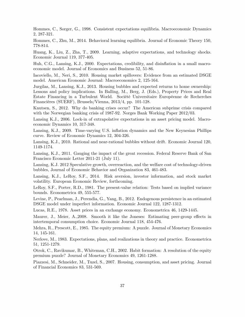
Hommes, C., Sorger, G., 1998. Consistent expectations equilibria. Macroeconomic Dynamics2, 287-321.
Hommes, C., Zhu, M., 2014. Behavioral learning equilibria. Journal of Economic Theory 150,778-814.
Huang, K., Liu, Z., Zha, T., 2009. Learning, adaptive expectations, and technology shocks.Economic Journal 119, 377-405.
Huh, C.G., Lansing, K.J., 2000. Expectations, credibility, and disinflation in a small macro-economic model. Journal of Economics and Business 52, 51-86.
Iacoviello, M., Neri, S., 2010. Housing market spillovers: Evidence from an estimated DSGEmodel. American Economic Journal: Macroeconomics 2, 125-164.
Jurgilas, M., Lansing, K.J., 2013. Housing bubbles and expected returns to home ownership:Lessons and policy implications. In Balling, M., Berg, J. (Eds.), Property Prices and RealEstate Financing in a Turbulent World. Société Universitaire Européenne de RecherchesFinancières (SUERF), Brussels/Vienna, 2013/4, pp. 101-128.
Knutsen, S., 2012. Why do banking crises occur? The American subprime crisis comparedwith the Norwegian banking crisis of 1987-92. Norges Bank Working Paper 2012/03.
Lansing K.J., 2006. Lock-in of extrapolative expectations in an asset pricing model. Macro-economic Dynamics 10, 317-348.
Lansing, K.J., 2009. Time-varying U.S. inflation dynamics and the New Keynesian Phillipscurve. Review of Economic Dynamics 12, 304-326.
Lansing, K.J., 2010. Rational and near-rational bubbles without drift. Economic Journal 120,1149-1174.
Lansing, K.J., 2011. Gauging the impact of the great recession. Federal Reserve Bank of SanFrancisco Economic Letter 2011-21 (July 11).
Lansing, K.J. 2012 Speculative growth, overreaction, and the welfare cost of technology-drivenbubbles, Journal of Economic Behavior and Organization 83, 461-483.
Lansing, K.J., LeRoy, S.F., 2014. Risk aversion, investor information, and stock marketvolatility. European Economic Review, forthcoming.
LeRoy, S.F., Porter, R.D., 1981. The present-value relation: Tests based on implied variancebounds. Econometrica 49, 555-577.
Levine, P., Pearlman, J., Perendia, G., Yang, B., 2012. Endogenous persistence in an estimatedDSGE model under imperfect information. Economic Journal 122, 1287-1312.
Lucas, R.E., 1978. Asset prices in an exchange economy. Econometrica 46, 1429-1445.
Maurer, J., Meier, A.,2008. Smooth it like the Joneses: Estimating peer-group effects inintertemporal consumption choice. Economic Journal 118, 454-476.
Mehra, R., Prescott, E., 1985. The equity premium: A puzzle. Journal of Monetary Economics14, 145-161.
Nerlove, M., 1983. Expectations, plans, and realizations in theory and practice. Econometrica51, 1251-1279.
Otrok, C., Ravikumar, B., Whiteman, C.H., 2002. Habit formation: A resolution of the equitypremium puzzle? Journal of Monetary Economics 49, 1261-1288.
Piazzesi, M., Schneider, M., Tuzel, S., 2007. Housing, consumption, and asset pricing. Journalof Financial Economics 83, 531-569.
37
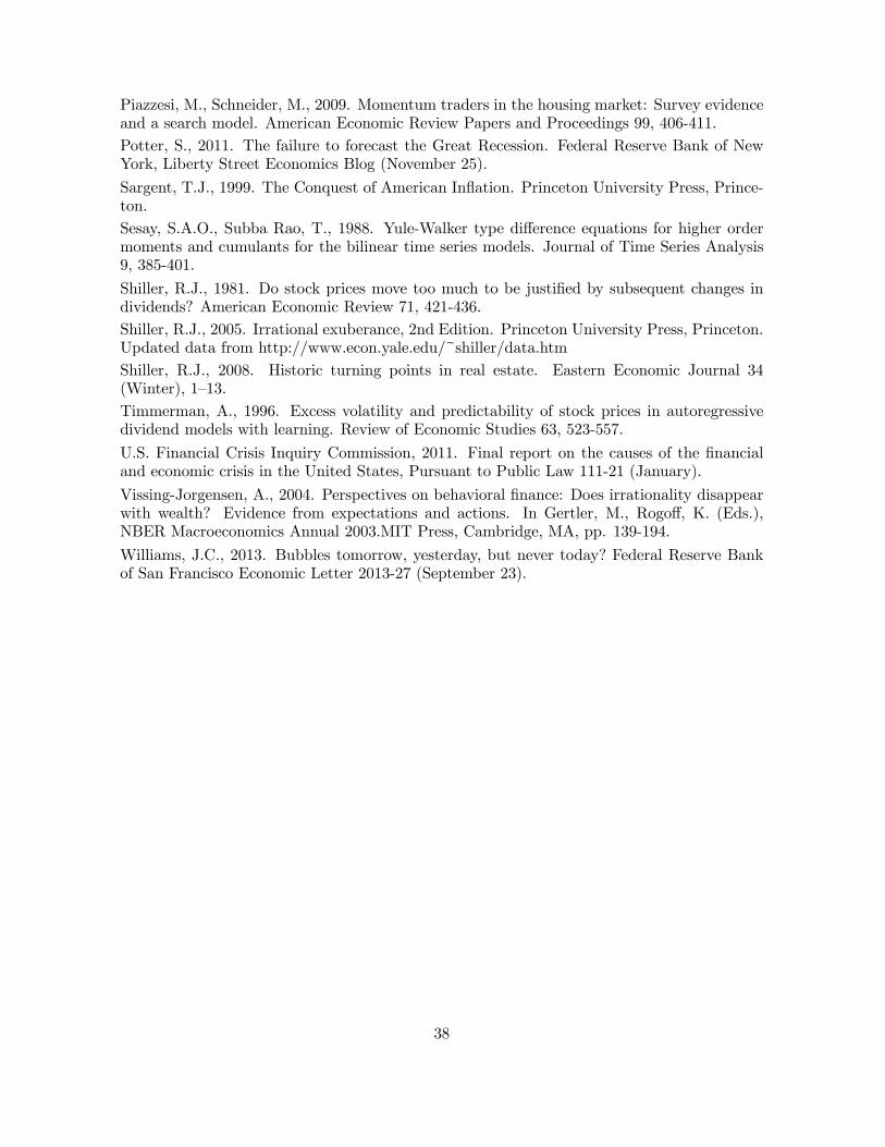
Piazzesi, M., Schneider, M., 2009. Momentum traders in the housing market: Survey evidenceand a search model. American Economic Review Papers and Proceedings 99, 406-411.
Potter, S., 2011. The failure to forecast the Great Recession. Federal Reserve Bank of NewYork, Liberty Street Economics Blog (November 25).
Sargent, T.J., 1999. The Conquest of American Inflation. Princeton University Press, Prince-ton.
Sesay, S.A.O., Subba Rao, T., 1988. Yule-Walker type difference equations for higher ordermoments and cumulants for the bilinear time series models. Journal of Time Series Analysis9, 385-401.
Shiller, R.J., 1981. Do stock prices move too much to be justified by subsequent changes individends? American Economic Review 71, 421-436.
Shiller, R.J., 2005. Irrational exuberance, 2nd Edition. Princeton University Press, Princeton.Updated data from http://www.econ.yale.edu/~shiller/data.htm
Shiller, R.J., 2008. Historic turning points in real estate. Eastern Economic Journal 34(Winter), 1—13.
Timmerman, A., 1996. Excess volatility and predictability of stock prices in autoregressivedividend models with learning. Review of Economic Studies 63, 523-557.
U.S. Financial Crisis Inquiry Commission, 2011. Final report on the causes of the financialand economic crisis in the United States, Pursuant to Public Law 111-21 (January).
Vissing-Jorgensen, A., 2004. Perspectives on behavioral finance: Does irrationality disappearwith wealth? Evidence from expectations and actions. In Gertler, M., Rogoff, K. (Eds.),NBER Macroeconomics Annual 2003.MIT Press, Cambridge, MA, pp. 139-194.
Williams, J.C., 2013. Bubbles tomorrow, yesterday, but never today? Federal Reserve Bankof San Francisco Economic Letter 2013-27 (September 23).
38


![Time-varying jump tails - Duke Universitypublic.econ.duke.edu/~boller/Published_Papers/joe_14.pdf · varying± ± ± ± ± − (+ −]) ± (+ − ±, =,..., −] = −, −] = −,),](https://img.pdfslide.us/doc/110x75/5f9eb1e298e27c43de4b3c12/time-varying-jump-tails-duke-bollerpublishedpapersjoe14pdf-varying-.jpg)