Hourly Global Solar Radiation Estimates on a Horizontal Plane

Journal of Physical Science, Vol. 21(2), 51–66, 2010 51

Hourly Global Solar Radiation Estimates on a Horizontal Plane

Abdul Majeed Muzathik1*

, Wan Mohd Norsani Wan Nik1,

Khalid Samo1 and Mohd. Zamri Ibrahim

2

1Department of Maritime Technology, Faculty of Maritime Studies and Marine Science,

2Department of Engineering Science, Faculty of Science and Technology,

University Malaysia Terengganu, 21030 Kuala Terengganu, Malaysia

*Corresponding author: [email protected]

Abstract: The hourly global solar radiation (It) model strongly depends on the climatic

characteristics of a considered site. In this paper, six empirical models were used to

estimate the It from daily radiation on the eastern coast of Malaysia. The measured It

data were obtained from the Malaysian Meteorology Department for the period of 2004–

2008. In order to determine the performance of the models, the statistical parameters,

normalised mean bias error (NMBE), normalised root mean square error (NRMSE),

correlation coefficient (r), and a t-test were used. The It values were calculated by using

the selected models. The results were compared with the measured data. This study finds

that the Collares-Pereira and Rabl model performed better than the other models.

Keywords: Collares-Pereira and Rabl model, global solar radiation, hourly solar

radiation (It) models, statistical tests, solar energy design

Abstrak: Pilihan model sinaran solar global perjam (It) adalah sangat bergantung

kepada ciri-ciri iklim lokasi yang ditentukan. Dalam kertas kerja ini, enam model

empirikal digunakan untuk menganggar It dari sinaran harian di pantai timur Malaysia.

It yang diukur diperolehi dari Jabatan Meteorologi Malaysia bagi jangka masa 2004–

2008. Bagi menentukan prestasi model, parameter statistik, ralat pincang purata

ternormal (NMBE), ralat punca ganda dua ternormal (NRMSE), pekali korelasi (r) dan

ujian t digunakan. Nilai It dihitung menggunakan model-model tersebut dan keputusan

dibandingkan dengan data yang diukur. Kajian ini mendapati bahawa model Collares-

Pereira dan Rabl adalah merupakan model yang terbaik.

Kata kunci: model Collares-Pereira dan Rabl, sinaran solar global, model sinaran solar

perjam (It), ujian statistik, rekabentuk/corak tenaga solar

1. INTRODUCTION

The data on solar radiation and its components at a given location are

essential for studies of solar energy. In other words, reasonably accurate

knowledge of the availability of solar resources at a given place is required. The

average values for the hourly, daily and monthly global irradiation on a

horizontal surface are needed for many applications of solar energy designs.1–5

mailto:[email protected]

Global Solar Radiation Estimates on a Horizontal Plane 52

Malaysia is a country that has abundant solar energy. The annual average

daily solar irradiations for Malaysia have a magnitude of 4.21–5.56 kWhm−2

, and

the sunshine duration is more than 2,200 hours per year.6 Unfortunately, for

many developing countries such as Malaysia, solar radiation measurements are

not easily available due to high equipment and maintenance costs and the

calibration requirements of the measuring equipment. A solution to this problem

is to estimate solar radiation by using a model. Indeed, the prediction of the

hourly global solar radiation, It, for a given day was the target of many research

attempts.7–16

Mean It values are useful for problems such as the effective and reliable

sizing of solar power systems (PV generators) and the management of solar

energy sources in relation to the power loads that must be met (output of the PV

systems affected by meteorological conditions). Modelling solar radiation also

provides an understanding of the dynamics of solar radiation, and it is clearly of

great value in the design of solar energy conversion systems.

The main objective of this paper is to validate the available models that

predict the It on a horizontal surface against the measured dataset for the Kuala

Terengganu site in Malaysia and, thereby, to retain the most accurate model. The

models that are considered for comparison and examination are as follows: the

Jain model,13,14

the Baig et al. model,10

a new approach to the Jain and Baig

models,16

the S. Kaplanis model15,16

and the Collares-Pereira and Rabl model.11

We first performed a literature review of the existing models and created a

description of each model. This step was followed by a statistical comparison of

the hourly retained models to the measured data that were obtained from the

Terengganu state.

2. EXPERIMENTAL

2.1. The Models

2.1.1 The Jain model

Jain13,14

proposed a Gaussian function to fit the recorded data and

established the following relation for global irradiation:


2

2

1 12= exp

2π 2t

tr

σ σ

(1)

where tr is the ratio of hourly to daily global radiation, t is the true solar time in

hours, and σ is defined by:

( 12)

1=

2t t

σr

(2)

where tr (t = 12) is the hourly ratio of the global irradiation at the midday true

solar time.

From the hourly data, taking I (t = 12) and the daily data, nH , we may

determine σ from equation (2). Then, from equation (1), the tr values are

obtained so as to provide:

.t t nI r H

(3)

2.1.2 The Baig model

The Baig et al.10

model modified Jain’s model to fit the recorded data

during the starting and ending periods of a given day better. In this model, tr is

estimated by:

2

2 1

1 12 12

= exp cos 180 2 2 2

to

t tr

sσ π σ

(4)

oS is the daily length of a day, n, at a specific site, and it is defined by:

12= cos tan tan

15oS φ δ

(5)

where φ and δ are the latitude of the considered site and the solar declination,

respectively. The declination angle is defined by:

= 23.45 sin 360 n + 284 / 365 δ

(6)


2.1.3 A new approach to the Jain and Baig models

This work proposes a different approach for determining σ without using

the values of I (t = 12), which was proposed by S. Kaplanis.16

Two versions of

this approach are presented because this approach concerns the determination

of σ.

The first approach: The day length, ,oS of a day, n, as determined from

equation (5), is equated with the time-distance between the points, where the

tangents at the two turning points of the hypothetical Gaussian distribution,

which fits the hourly It data, intersect the (temporal) hour, or t, axis. These two

points are at a ±2σ distance from the axis of origin. Then, σ is related directly to

oS by 4 σ.

The second approach: If one draws a tangent at the two points that

correspond to the full width at the half-maximum of a Gaussian curve, it can be

determined that the tangent at each point intersects the horizontal axis, i.e., the

hour, or t, axis at the points of ±2.027σ instead of at ±2σ, as in the first version.

Hence, in this case, oS = 4.054 σ or σ = 0.246 .oS In these new approaches, either

method for determining σ does not require any recorded data.

2.1.4 The Kaplanis model

In this model, a and b are parameters that should be determined for any

site and any day, n. Their determination is as follows:

2Let, = + .cos 24

π.t I a b

(7)

Integrating equation (7) over t, from sunrise, or ,t sr to sunset, or ,t ss one obtains:

122 .24

= H = 2 + sin 24

tss

sssr

tsr

ttb

Idt a

(8)

A boundary condition provides a relationship between a and b. That is, at t = ,t ss

I = 0. Hence, from equation (7), one obtains:

2 π / 24 + cos = 0tssa b (9)

Equations (8) and (9) provide the values of a and b by using the H values that are

taken from the recorded data.


2.1.5 The Collares-Pereira and Rabl model

Collares-Pereira and Rabl11

proposed a semi-empirical expression for ,tr

as follows:

=

cos cos + cos

24 sin cos 2π. / 360

s

ts ss

w wπr x y w

w ww

(10)

This equation yields the coefficients given by:

60 = 0.409 + 0.5016sin swx

(11)

60 = 0.6609 0.47676sin swy (12)

where w is the hour angle in degrees for the considered hour, and sw is the sunset

hour angle in degrees calculated by the following equation:

1

= cos tan tan ow (φ) (δ) (13)

where φ is the latitude of the considered site and δ is the solar declination angle

calculated for the representative day of the month.

2.2 Method of Statistical Comparison

There are numerous studies in the literature that address the assessment

and comparison of It estimation models.17–20

The most popular statistical

parameters are the normalised mean bias error (NMBE) and the normalised root

mean square error (NRMSE). In this study, to evaluate the accuracy of the

estimated data from the models described above, some statistical tests [the

NMBE, NRMSE and coefficient of correlation (r)] to verify the linear

relationship between the predicted and measured values are used. For better data

modelling, these statistics should be close to zero, but r should approach one as

closely as possible. In addition, the t-test for the models was carried out to

determine the statistical significance of the predicted values by the models.


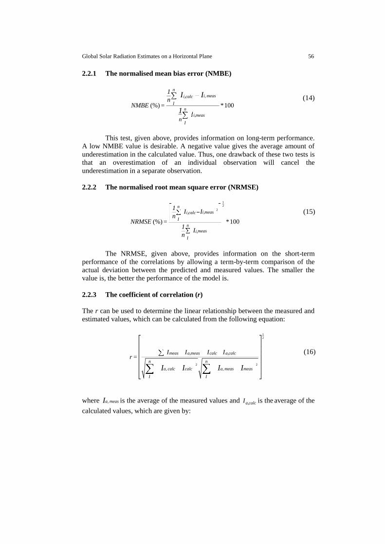
2.2.1 The normalised mean bias error (NMBE)

(%) 100

n

i, measi,calc

I

n

i,meas

In

1

nNMBE = *

I I

1

(14)

This test, given above, provides information on long-term performance.

A low NMBE value is desirable. A negative value gives the average amount of

underestimation in the calculated value. Thus, one drawback of these two tests is

that an overestimation of an individual observation will cancel the

underestimation in a separate observation.

2.2.2 The normalised root mean square error (NRMSE)

2

12

(%) 100

n

i,measi,calc

I

n

measi,

I

1I I

nNRMSE = *

1I

n

(15)

The NRMSE, given above, provides information on the short-term

performance of the correlations by allowing a term-by-term comparison of the

actual deviation between the predicted and measured values. The smaller the

value is, the better the performance of the model is.

2.2.3 The coefficient of correlation (r)

The r can be used to determine the linear relationship between the measured and

estimated values, which can be calculated from the following equation:

2 2

12

meas a,meas calc a,calc

n n

a, calc calc a, meas meas

I I

I I I I r =

I I I I

(16)

where a, measI is the average of the measured values and a,calcI is the average of the

calculated values, which are given by:


and = .n n

meas calca,meas a,calcI I

1 1I

n nI I = I

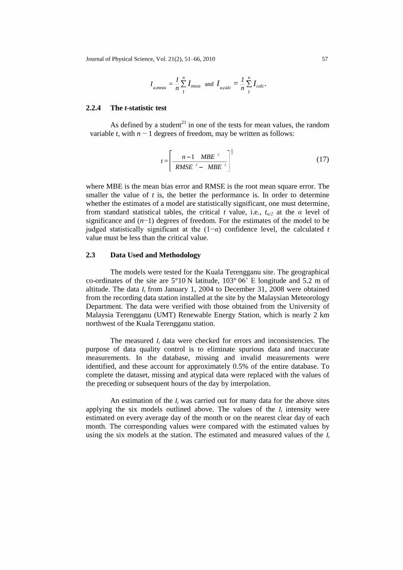
2.2.4 The t-statistic test

As defined by a student21

in one of the tests for mean values, the random

variable t, with n − 1 degrees of freedom, may be written as follows:

2

2 2

12

1

n MBEt =

RMSE MBE

(17)

where MBE is the mean bias error and RMSE is the root mean square error. The

smaller the value of t is, the better the performance is. In order to determine

whether the estimates of a model are statistically significant, one must determine,

from standard statistical tables, the critical t value, i.e., tα/2 at the α level of

significance and (n−1) degrees of freedom. For the estimates of the model to be

judged statistically significant at the (1−α) confidence level, the calculated t

value must be less than the critical value.

2.3 Data Used and Methodology

The models were tested for the Kuala Terengganu site. The geographical

co-ordinates of the site are 5°10’N latitude, 103°

06’ E longitude and 5.2 m of

altitude. The data It from January 1, 2004 to December 31, 2008 were obtained

from the recording data station installed at the site by the Malaysian Meteorology

Department. The data were verified with those obtained from the University of

Malaysia Terengganu (UMT) Renewable Energy Station, which is nearly 2 km

northwest of the Kuala Terengganu station.

The measured It data were checked for errors and inconsistencies. The

purpose of data quality control is to eliminate spurious data and inaccurate

measurements. In the database, missing and invalid measurements were

identified, and these account for approximately 0.5% of the entire database. To

complete the dataset, missing and atypical data were replaced with the values of

the preceding or subsequent hours of the day by interpolation.

An estimation of the It was carried out for many data for the above sites

applying the six models outlined above. The values of the It intensity were

estimated on every average day of the month or on the nearest clear day of each

month. The corresponding values were compared with the estimated values by

using the six models at the station. The estimated and measured values of the It


intensity were analysed using the NMBE, NRMSE, r values and t-test statistical

tests for the representative days for 12 months throughout the year. A programme

was developed using MATLAB to provide and plot the It estimations. The

models were checked with repeated runs and different sequences, as is required

for the prediction of It.

3. RESULTS AND DISCUSSION

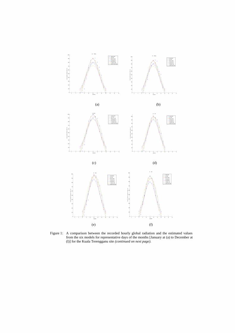
Figure 1 shows the recorded and estimated values from the selected six

models of It for representative days of the months for the Kuala Terengganu sites.

During solar noon, the Jain and Baig et al. models both gave the same values

because these models are based on the solar noon measured values. The

estimates of the Jain and Baig et al. models of the It show symmetry around the

solar noon, as imposed by the Gaussian fitting function. The Jain and Baig et al.

Models seem to provide very reliable performance close to solar noon, which is

due to the solar noon recorded values required by the models. For the rest of the

day, the estimates of It vary within the standard deviation. The estimated values

of the Jain models were almost always less than the measured values for the main

part of the day. The mismatch was much wider during the early and late hours of

the day as the Gaussian function became zero at infinity (time), because there is

practically no radiation before sunrise and after sunset.

The Kaplanis model gives an underestimation of about 10% in the worst

cases, which are in January, October and December at solar noon. For the rest of

the day, the It estimates are close to the measured values. The Collares-Pereira

and Rabl model gives an overestimation of about 8%–10% in the worst cases,

which are in May and September at solar noon. For the rest of the day, the It

estimates are close to the measured values. The new approach to the first and

second approaches (henceforth known as new approaches) from Jain and Baig

gives the same estimates of It because both models are based on the theoretical σ

values, which are almost the same values in both cases (σ = 0.25 in the first

approach and σ = 0.246 in the second approach). The new approaches for Jain

and Baig gives an overestimation of about 5%–8% in the worst cases, which are

in January and February, and an underestimation of about 5% (in the worst cases),

which are in July and December at solar noon. For the rest of the day, the It

estimates are close to the recorded values. To make a comparison among the

models, the estimated and measured values were compared for each

representative day of the various months. The statistical summary of the

performance of the combination of the different test indicators is presented in

Table 1 for the It at the Kuala Terengganu site.


The estimates of the It that were obtained by the models for most months

are close to the measured values. The difference between the measured and

estimated values was 17.00% (at the maximum) for the Kuala Terengganu site.

For the It, the results presented in Table 1 show that the Collares-Pereira and Rabl

model generally leads to the best results. For the Kuala Terengganu site, the

NRMSE values that were obtained by using this model were generally 8%–20%.

This model appears to perform well at the Kuala Terengganu site. For the Jain

and Baig models, the new approaches were carried out. This new approach and

the Kaplanis model resulted in the largest NRMSE with values that were

generally greater than 25%.

In addition, the low NMBE values are particularly remarkable. The

NMBE values show that the Collares-Pereira and Rabl model generally yields

the best results. The negative NMBE values presented in Table 1 show that an

underestimation of It occurs during the period of January to March and

September to December, whereas overestimation of It occurs during the period of

April to August with the Collares-Pereira and Rabl model.

The Jain, Baig, and the Kaplanis models present NMBE values that are

higher than those obtained by the Collares-Pereira and Rabl model. The new

approaches for Jain and Baig models yields smaller negative NMBE values. This

result indicates that there is an underestimation during the entire period of the

year, even though the NRMSE values are very high for these models. From the

table, it can be seen that the average r of the Collares-Pereira and Rabl model is

0.98. This result indicates that the Collares-Pereira and Rabl model accounts well

for the variability in the It. The average r of the other models is around 0.96. It is

clear that the deviations between the measured and estimated values of these five

models are larger than those of the Collares-Pereira and Rabl model. However,

all six models may be accepted if one considers only the coefficient of

correlation between the measured and estimated values.

In addition, a t-test for the models was carried out to determine the

statistical significance of the estimated values from the models. The models

having a lower t value than the t critical value are statistically acceptable models.

From the standard statistical tables, the critical t value is 2.1788 at a 5% level of

significance (95% confidence level) with 12 degrees of freedom. According to

the t-tests given in Table 1, the evaluations of the models are good for the Kuala

Terengganu site. In particular, the Jain model and the new approaches for Jain

and Baig models give the best results for the site.

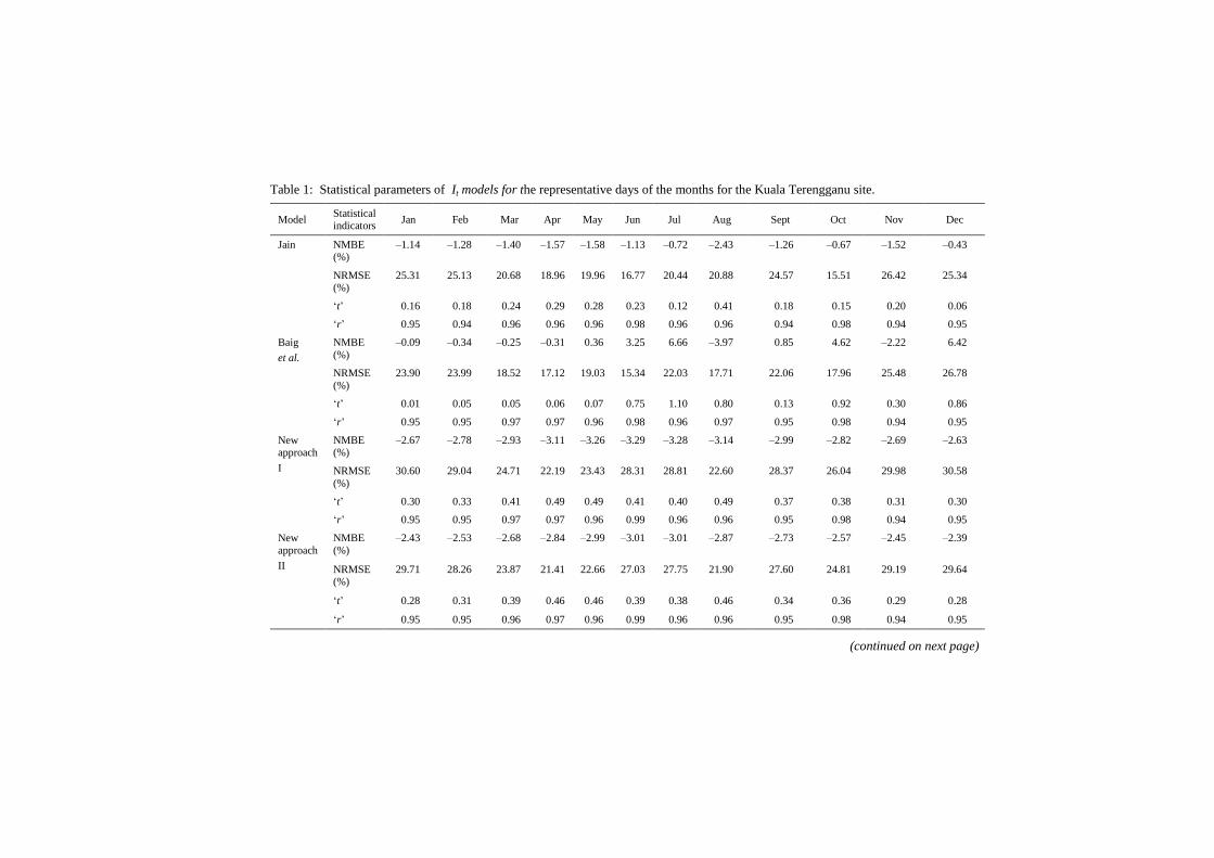
Table 1: Statistical parameters of It models for the representative days of the months for the Kuala Terengganu site.

Model Statistical indicators

Jan Feb Mar Apr May Jun Jul Aug Sept Oct Nov Dec

Jain NMBE (%)

–1.14 –1.28 –1.40 –1.57 –1.58 –1.13 –0.72 –2.43 –1.26 –0.67 –1.52 –0.43

NRMSE (%)

25.31 25.13 20.68 18.96 19.96 16.77 20.44 20.88 24.57 15.51 26.42 25.34

‘t’ 0.16 0.18 0.24 0.29 0.28 0.23 0.12 0.41 0.18 0.15 0.20 0.06

‘r’ 0.95 0.94 0.96 0.96 0.96 0.98 0.96 0.96 0.94 0.98 0.94 0.95

Baig

et al.

NMBE

(%)

–0.09 –0.34 –0.25 –0.31 0.36 3.25 6.66 –3.97 0.85 4.62 –2.22 6.42

NRMSE

(%)

23.90 23.99 18.52 17.12 19.03 15.34 22.03 17.71 22.06 17.96 25.48 26.78

‘t’ 0.01 0.05 0.05 0.06 0.07 0.75 1.10 0.80 0.13 0.92 0.30 0.86

‘r’ 0.95 0.95 0.97 0.97 0.96 0.98 0.96 0.97 0.95 0.98 0.94 0.95

New approach

I

NMBE (%)

–2.67 –2.78 –2.93 –3.11 –3.26 –3.29 –3.28 –3.14 –2.99 –2.82 –2.69 –2.63

NRMSE

(%)

30.60 29.04 24.71 22.19 23.43 28.31 28.81 22.60 28.37 26.04 29.98 30.58

‘t’ 0.30 0.33 0.41 0.49 0.49 0.41 0.40 0.49 0.37 0.38 0.31 0.30

‘r’ 0.95 0.95 0.97 0.97 0.96 0.99 0.96 0.96 0.95 0.98 0.94 0.95

New

approach

II

NMBE

(%)

–2.43 –2.53 –2.68 –2.84 –2.99 –3.01 –3.01 –2.87 –2.73 –2.57 –2.45 –2.39

NRMSE (%)

29.71 28.26 23.87 21.41 22.66 27.03 27.75 21.90 27.60 24.81 29.19 29.64

‘t’ 0.28 0.31 0.39 0.46 0.46 0.39 0.38 0.46 0.34 0.36 0.29 0.28

‘r’ 0.95 0.95 0.96 0.97 0.96 0.99 0.96 0.96 0.95 0.98 0.94 0.95

(continued on next page)

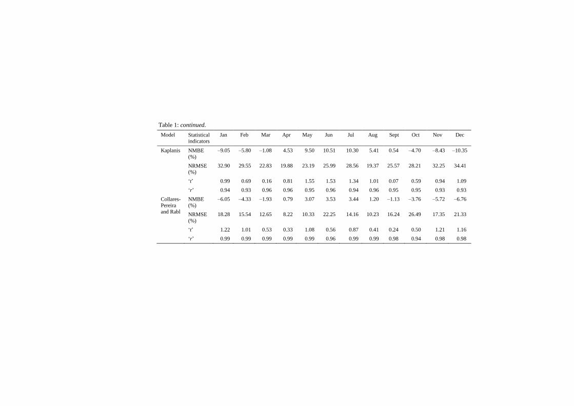
Table 1: continued.

Model Statistical indicators

Jan Feb Mar Apr May Jun Jul Aug Sept Oct Nov Dec

Kaplanis NMBE

(%)

–9.05 –5.80 –1.08 4.53 9.50 10.51 10.30 5.41 0.54 –4.70 –8.43 –10.35

NRMSE (%)

32.90 29.55 22.83 19.88 23.19 25.99 28.56 19.37 25.57 28.21 32.25 34.41

‘t’ 0.99 0.69 0.16 0.81 1.55 1.53 1.34 1.01 0.07 0.59 0.94 1.09

‘r’ 0.94 0.93 0.96 0.96 0.95 0.96 0.94 0.96 0.95 0.95 0.93 0.93

Collares-Pereira

and Rabl

NMBE (%)

–6.05 –4.33 –1.93 0.79 3.07 3.53 3.44 1.20 –1.13 –3.76 –5.72 –6.76

NRMSE

(%)

18.28 15.54 12.65 8.22 10.33 22.25 14.16 10.23 16.24 26.49 17.35 21.33

‘t’ 1.22 1.01 0.53 0.33 1.08 0.56 0.87 0.41 0.24 0.50 1.21 1.16

‘r’ 0.99 0.99 0.99 0.99 0.99 0.96 0.99 0.99 0.98 0.94 0.98 0.98

2 4 6 8 10 12 14 16 18 20 22 240

100

200

300

400

500

600

700

800

900

1000(a) January

day hours

hourly g

lobal ra

dia

tion (

Wm

-2)

measured data

Jain model

Baig et al model

new approaches 1

new approaches 2

S. Kaplanis model

Collares-Pereira model

2 4 6 8 10 12 14 16 18 20 22 240

100

200

300

400

500

600

700

800

900

1000(b) February

day hours

hourly g

lobal ra

dia

tion (

Wm

-2)

measured data

Jain model

Baig et al model

new approaches 1

new approaches 2

S. Kaplanis model


(a) (b)

2 4 6 8 10 12 14 16 18 20 22 240

100

200

300

400

500

600

700

800

900

1000(c) March

day hours

hourly g

lobal ra

dia

tion (

Wm

- 2)

measured data

Jain model

Baig et al model

new approaches 1

new approaches 2

S. Kaplanis model


2 4 6 8 10 12 14 16 18 20 22 240

100

200

300

400

500

600

700

800

900

1000

(d) April

day hours

hourly g

lobal ra

dia

tion (

Wm

-2)

measured data

Jain model

Baig et al model

new approaches 1

new approaches 2

S. Kaplanis model


(c) (d)

2 4 6 8 10 12 14 16 18 20 22 240

100

200

300

400

500

600

700

800

900

1000(e) May

day hours

hourly

glo

bal radia

tio

n (W

m-2)

measured data

Jain model

Baig et al model

new approaches 1

new approaches 2

S. Kaplanis model


2 4 6 8 10 12 14 16 18 20 22 240

100

200

300

400

500

600

700

800

900

1000(f) June

day hours

hourly

glo

bal radia

tio

n (W

m-2)

measured data

Jain model

Baig et al model

new approaches 1

new approaches 2

S. Kaplanis model


(e) (f)

Figure 1: A comparison between the recorded hourly global radiation and the estimated values

from the six models for representative days of the months [January at (a) to December at

(l)] for the Kuala Terengganu site (continued on next page).

2 4 6 8 10 12 14 16 18 20 22 240

100

200

300

400

500

600

700

800

900

1000

(g) July

day hours

hourly g

lobal ra

dia

tion (

Wm

-2)

measured data

Jain model

Baig et al model

new approaches 1

new approaches 2

S. Kaplanis model


2 4 6 8 10 12 14 16 18 20 22 240

100

200

300

400

500

600

700

800

900

1000(h) August

day hours

hourly g

lobal ra

dia

tion (

Wm

-2)

measured data

Jain model

Baig et al model

new approaches 1

new approaches 2

S. Kaplanis model


(g) (h)

2 4 6 8 10 12 14 16 18 20 22 240

100

200

300

400

500

600

700

800

900

1000(i) September

day hours

hourly

glo

bal radia

tio

n (W

m-2)

measured data

Jain model

Baig et al model

new approaches 1

new approaches 2

S. Kaplanis model


2 4 6 8 10 12 14 16 18 20 22 240

100

200

300

400

500

600

700

800

900

1000(j) October

day hours

hourly g

lobal ra

dia

tion (

Wm

-2)

measured data

Jain model

Baig et al model

new approaches 1

new approaches 2

S. Kaplanis model


(i) (j)

2 4 6 8 10 12 14 16 18 20 22 240

100

200

300

400

500

600

700

800

900

1000(k) November

day hours

hourly

glo

bal radia

tio

n (W

m-2)

measured data

Jain model

Baig et al model

new approaches 1

new approaches 2

S. Kaplanis model


2 4 6 8 10 12 14 16 18 20 22 240

100

200

300

400

500

600

700

800

900

1000(l) December

day hours

hourly g

lobal ra

dia

tion (

Wm

-2)

measured data

Jain model

Baig et al model

new approaches 1

new approaches 2

S. Kaplanis model


(k) (l)

Figure 1: continued.


Finally, the estimated values of It at the Kuala Terengganu site are in

favourable agreement with the measured values for the It for all of the months in

the year. It was found that the Collares-Pereira and Rabl model shows the best

results among all of the models for the site. This is due to the low values of the

Collares-Pereira and Rabl model for the NMBE, NRMSE, and the t-test, and the

fact that the coefficient of correlation is 0.98. Therefore, based on this study, the

Collares-Pereira and Rabl model can be recommended for use in estimating the It

at the Kuala Terengganu site in Malaysia and also for places with similar climatic

conditions.

4. CONCLUSION

According to the research based on the statistical parameters of the

normalised mean bias error (NMBE), normalised root mean square error

(NRMSE), coefficient of correlation (r) and a t-test, the Collares-Pereira and Rabl

model is the most accurate one for estimating the hourly global solar radiation, It

for Kuala Terengganu in Malaysia and for other locations that exhibit similar

climatic conditions. Furthermore, the result of this analysis could be used in the

design of solar energy applications and other related mechanisms.

5. ACKNOWLEDGEMENT

The authors would like to thank the Malaysian Meteorological

Department for providing the data for this research. In addition, the authors

would like to thank the Maritime Technology and the Engineering Science

Departments at University of Malaysia Terengganu (UMT) for providing

technical and financial support.

6. REFERENCES

1. Almorox, J. & Hontoria, C. (2004). Global solar radiation estimation

using sunshine duration in Spain. Energy Convers. Manage., 45(9–10),

1529–1535.

2. Sopian, K. & Othman, M. Y. (1992). Estimates of monthly average daily

global solar radiation in Malaysia. Renewable Energy, 2(3), 319–325.

3. Li, D. H. W. & Lam, J. C. (2000). Solar heat gain factors and the

implications for building designs in subtropical regions. Energy Build.,

32(1), 47–55.


4. Wong, L. T. & Chow, W. K. (2001). Solar radiation model. Appl. Energy,

69(3), 191–224.

5. Kumar, R. & Umanand, L. (2005). Estimation of global radiation using

clearness index model for sizing photovoltaic system. Renewable Energy,

30(15), 2221–2233.

6. Muzathik, A. M., Wan Nik, W. B., Samo, K. B. & Ibrahim, M. Z. (2010).

Reference solar radiation year and some dimatology aspects of East

Coast of West Malaysia. Am. J. Eng. Appl. Sci., 3(2), 293–299.

7. Zekai, S. (2008). Solar energy fundamentals and modeling techniques:

Atmosphere, environment, climate change and renewable energy.

London: Springer-Verlag.

8. Aguiar, R. & Collares-Perreira, M. (1992a). Statistical properties of

hourly global solar radiation. Sol. Energy, 48(3), 157–167.

9. _______. (1992b). TAG: A time dependent autoregressive Gaussian

model for generating synthetic hourly radiation, Sol. Energy, 49(3), 167–

174.

10. Baig, A., Achter, P. & Mufti, A. (1991). A novel approach to estimate the

clear day global radiation. Renewable Energy, 1(1), 119–123.

11. Collares-Pereira, M. & Rabl. (1979). The average distribution of solar

radiation-correlation between diffuse and hemispherical and daily and

hourly insolation values. Sol. Energy, 22(2), 155–164.

12. Gueymard, C. (1993). Critical analysis and performance assessment of

clear solar sky irradiance models using theoretical and measured data. Sol.

Energy, 51(2), 121–138.

13. Jain, P. C. (1984). Comparison of techniques for the estimation of daily

global irradiation and a new technique for the estimation of global

irradiation. Sol. Wind Technol., 1(2), 123–134.

14. _______. (1988). Estimation of monthly average hourly global and diffuse

irradiation, Sol. Wind Technol., 5(1), 7–14.

15. Kaplanis, S. & Kaplain, E. (2007). A model to predict expected mean and

stochastic hourly global solar radiation I (h;nj) values. Renewable Energy,

32(8), 1414–1425.

16. Kaplanis, S. N. (2006). New methodologies to estimate the hourly global

solar radiation: Comparisons with existing models. Renewable Energy,

31(6), 781–790.

17. Koussa, M., Malek, A. & Haddadi, M. (2009). Statistical comparison of

monthly mean hourly and daily diffuse and global solar irradiation

models and a Simulink program development for various Algerian

climates. Energy Convers. Manage., 50(5), 1227–1235.

18. Bulut, H. & Büyükalaca, O. (2007). Simple model for the generation of

daily global solar-radiation data in Turkey. Appl. Energy, 84(5), 477–491.

19. Gueymard, C. (2000). Prediction and performance assessment of mean

hourly solar radiation, Sol. Energy, 68(3), 285–303.


20. Şenkal, O. & Kuleli, T. (2009). Estimation of solar radiation over Turkey

using artificial neural network and satellite data. Appl. Energy, 86(7–8),

1222–1228.

21. Box, J. F. (1987). Guinness, Gosset, Fishes, and small samples.

Statistical Sci., 2(1), 45–52.

Documents

Hourly Global Solar Radiation Estimates on a Horizontal Plane