Geoscience Frontiers xxx (xxxx) xxx

HOSTED BY Contents lists available at ScienceDirect

Geoscience Frontiers

journal homepage: www.elsevier.com/locate/gsf

Research Paper

Resistivity of reservoir sandstones and organic rich shales on the BarentsShelf: Implications for interpreting CSEM data

Kim Senger a,*, Thomas Birchall a,b, Peter Betlem a,b, Kei Ogata c,d, Sverre Ohm a,e,Snorre Olaussen a, Renate S. Paulsen a,f

a Department of Arctic Geology, The University Centre in Svalbard, Longyearbyen, Norwayb Department of Geosciences, University of Oslo, Oslo, Norwayc Department of Earth Science, Vrije Universiteit, Amsterdam, Netherlandsd Now at Dipartimento di Scienze Della Terra, Dell’Ambiente e Delle Risorse (DISTAR), Universit�a Degli Studi di, Napoli Federico II, Napoli, Italye Department of Energy Resources, University of Stavanger, Stavanger, Norwayf Department of Geosciences, University of Tromsø – the Arctic University of Norway, Tromsø, Norway

A R T I C L E I N F O

Keywords:Barents ShelfPetroleumElectromagneticExplorationSource rocks

* Corresponding author.E-mail address: kim.senger@unis.no (K. Senger)Peer-review under responsibility of China Univ

https://doi.org/10.1016/j.gsf.2020.08.007Received 4 November 2019; Received in revised fo1674-9871/© 2021 China University of GeoscienceCC BY-NC-ND license (http://creativecommons.org/licenses/by-nc-nd/4.0/).

Please cite this article as: Senger, K. et al., ResiCSEM data, Geoscience Frontiers, https://doi

A B S T R A C T

Marine controlled source electromagnetic (CSEM) data have been utilized in the past decade during petroleumexploration of the Barents Shelf, particularly for de-risking the highly porous sandstone reservoirs of the UpperTriassic to Middle Jurassic Realgrunnen Subgroup. In this contribution we compare the resistivity response fromCSEM data to resistivity from wireline logs in both water- and hydrocarbon-bearing wells. We show that there is avery good match between these types of data, particularly when reservoirs are shallow. CSEM data, however, onlyprovide information on the subsurface resistivity. Careful, geology-driven interpretation of CSEM data is requiredto maximize the impact on exploration success. This is particularly important when quantifying the relative re-sistivity contribution of high-saturation hydrocarbon-bearing sandstone and that of the overlying cap rock. In thepresented case the cap rock comprises predominantly organic rich Upper Jurassic–Early Cretaceous shales of theHekkingen Formation (i.e. a regional source rock). The resistivity response of the reservoir and its cap rockbecome merged in CSEM data due to the transverse resistance equivalence principle. As a result of this, it isimperative to understand both the relative contributions from reservoir and cap rock, and the geological sig-nificance of any lateral resistivity variation in each of the units. In this contribution, we quantify the resistivity oforganic rich mudstone, i.e. source rock, and reservoir sandstones, using 131 exploration boreholes from theBarents Shelf. The highest resistivity (>10,000 Ωm) is evident in the hydrocarbon-bearing Realgrunnen Subgroupwhich is reported from 48 boreholes, 43 of which are used for this study. Pay zone resistivity is primarilycontrolled by reservoir quality (i.e. porosity and shale fraction) and fluid phase (i.e. gas, oil and water saturation).In the investigated wells, the shale dominated Hekkingen Formation exhibits enhanced resistivity compared to thebackground (i.e. the underlying and overlying stratigraphy), though rarely exceeds 20 Ωm. Marine mudstonestypically show good correlation between measured organic richness and resistivity/sonic velocity log signatures.We conclude that the resistivity contribution to the CSEM response from hydrocarbon-bearing sandstones out-weighs that of the organic rich cap rocks.

1. Introduction

Seismic data, which rely on mapping the acoustic impedance (i.e.velocity � density) contrasts of the subsurface (Cartwright and Huuse,2005), are routinely used to produce structural subsurface maps prior todrilling. The determination of subsurface fluids during petroleum

.ersity of Geosciences (Beijing).

rm 25 June 2020; Accepted 4 Aus (Beijing) and Peking University.

stivity of reservoir sandstones a.org/10.1016/j.gsf.2020.08.00

exploration is, however, challenging when using seismic data alone. Inparticular, it is difficult to discriminate reservoirs with a high gassaturation from those with low saturation (i.e. the "fizz gas" effect; e.g.,Han and Batzle, 2002). In contrast to sonic velocity, resistivity is onlyaffected when hydrocarbon saturation exceeds 60%–70% (Constable,2010; Hesthammer et al., 2010) and is the prime tool used to calculate

gust 2020Production and hosting by Elsevier B.V. This is an open access article under the

nd organic rich shales on the Barents Shelf: Implications for interpreting7

Fig. 1. Structural map of the study area, courtesy of NPD (2016). Wells with hydrocarbons within the Realgrunnen Subgroup are highlighted by green circles.

K. Senger et al. Geoscience Frontiers xxx (xxxx) xxx

water saturation in pay zone intervals. Resistivity has been measured invirtually all exploration boreholes since Schlumberger started wirelinelogging in 1927 (Johnson, 1962). Much can be learned from resistivitywireline logs to improve and calibrate the interpretation of controlledsource electromagnetic (CSEM) data. Furthermore, resistivity logsprovide a direct comparison to pre-drill derived resistivity from CSEMdata.

CSEM is primarily a marine data acquisition technique that has beenused by the petroleum industry since the early 2000s (Eidesmo et al.,2002; Ellingsrud et al., 2002). As resistivity logs are complementary toother wireline logs, CSEM data are complementary to seismic data.Acquisition of CSEM data typically relies on towing a high-poweredhorizontal electric dipole source approximately 30 m above the sea-floor to transmit a low-frequency electromagnetic signal through theseafloor (MacGregor and Tomlinson, 2014). Three-component nodalreceivers placed on the seafloor record the electric and magneticcomponents (Constable, 2010; Johansen and Gabrielsen, 2015; Mac-Gregor and Tomlinson, 2014). Inversion of CSEM data iteratively at-tempts to find an acceptable subsurface resistivity model that fits theactual measurements, thus providing subsurface resistivity cubes andprofiles. Interpretation of CSEM resistivity data is non-trivial and relieson understanding two aspects, namely (1) how CSEM data are acquiredand inverted, including careful consideration of the role played byCSEM sensitivity, and (2) what geological factors influence the sub-surface resistivity distribution. Johansen and Gabrielsen (2015) pro-vided a comprehensive overview of the acquisition, processing andinversion of CSEM and magnetotelluric (MT) data in hydrocarbonprospecting.

Typically, marine CSEM data are used to de-risk seismically-defined

2

prospects by identifying and characterizing laterally constrained, highresistive anomalies thought to be associated with hydrocarbon saturation(Fanavoll et al., 2014; Johansen and Gabrielsen, 2015; MacGregor et al.,2012; Stefatos et al., 2014). A number of CSEM-driven leads developedon the basis of high resistivity anomalies have also been defined (Cars-tens, 2018; Stefatos et al., 2014). However, resistive anomalies can alsobe related to other geological factors, for instance tight sandstones, tightcarbonates, mature source rocks, salt, fresh water, gas hydrates origneous intrusions (e.g., Alvarez et al., 2018; Barker and Baltar, 2016;Evans, 2007; Schwalenberg et al., 2017; Senger et al., 2017b; Spacapanet al., 2019; Tharimela et al., 2019).

The main benefit of using CSEM is to quantify the subsurface re-sistivity distribution prior to drilling. As with any exploration technique,CSEM has its limitations and interpreters must be aware of potentialpitfalls. One of the key aspects to consider with CSEM is its sensitivity to agiven target. Sensitivity is governed by the target size (i.e. area), targettransverse resistance (i.e. pay zone resistivity times pay zone thickness),target burial depth and structural and stratigraphic complexity of thebackground resistivity (MacGregor, 2012; MacGregor and Tomlinson,2014). If properly integrated into the exploration workflow, CSEM datacan be applied to de-risk prospects (Buland et al., 2011; Fanavoll et al.,2014; Gabrielsen et al., 2013), hydrocarbon saturation prediction prior todrilling (Løseth et al., 2014), optimizing a drilling strategy for a prospectportfolio (Zweidler et al., 2015), constraining gas hydrate systems(Tharimela et al., 2019; Weitemeyer et al., 2011), or delineating dis-coveries and constraining resource estimates (Baltar and Barker, 2015;Baltar and Roth, 2013). Many case studies where CSEM has been suc-cessfully used in exploration stem from the Barents Sea (e.g., Alvarezet al., 2018; Fanavoll et al., 2014; Gabrielsen et al., 2013; Granli et al.,

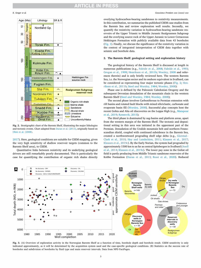
Fig. 2. Stratigraphic chart of the Barents Shelf, illustrating the major lithologiesand tectonic events. Chart adapted from Duran et al. (2013), originally based onOhm et al. (2008).

K. Senger et al. Geoscience Frontiers xxx (xxxx) xxx

2017). Here, geological conditions are suitable for CSEMmapping, giventhe very high sensitivity of shallow reservoir targets (common to theBarents Shelf area), to CSEM.

Quantitative links between resistivity and its underlying geologicaldrivers are still remarkably poorly documented. This is particularly thecase for quantifying the contribution of organic rich shales directly

Fig. 3. (A) Overview of exploration activity in the Norwegian Barents Shelf as a findicated approximately, as it will be determined by the acquisition system used aboreholes and subdivision of boreholes by fluid type and main reservoir intervals. D

3

overlying hydrocarbon-bearing sandstones to resistivity measurements.In this contribution, we summarize the published CSEM case studies fromthe Barents Sea and review exploration well results. Secondly, wequantify the resistivity variation in hydrocarbon-bearing sandstone res-ervoirs of the Upper Triassic to Middle Jurassic Realgrunnen Subgroupand the overlying source rock of the Upper Jurassic to Lower CretaceousHekkingen Formation with publicly available data from 43 boreholes(Fig. 1). Finally, we discuss the significance of the resistivity variation inthe context of integrated interpretation of CSEM data together withseismic and borehole data.

2. The Barents Shelf: geological setting and exploration history

The geological history of the Barents Shelf is discussed at length innumerous publications (e.g., Faleide et al., 2008; Faleide et al., 1993;Grogan et al., 1999; Henriksen et al., 2011b; Worsley, 2008 and refer-ences therein) and is only briefly reviewed here. The western BarentsSea, i.e. the Norwegian sector and its onshore equivalent in Svalbard, canbe considered as representing four major tectonic phases (Fig. 2; Hen-riksen et al., 2011b; Steel and Worsley, 1984; Worsley, 2008):

Phase one is defined by the Paleozoic Caledonian Orogeny and thesubsequent Devonian denudation of the mountain chain in the westernBarents Shelf (Steel and Worsley, 1984; Worsley, 2008);

The second phase involves Carboniferous to Permian extension withrift basins and rotated fault blocks with mixed siliciclastic, carbonate andevaporate basin fill (Worsley, 2008). Successful play concepts host therecent Gohta and Alta oil discoveries on the Loppa High (e.g., Matapouret al., 2019; Rønnevik, 2015);

The third phase is dominated by sag-basins and platform areas, apartfrom the western margin of the Barents Shelf. The tectonic and deposi-tional setting in this area was initiated in the uppermost part of thePermian. Denudation of the Uralide mountain belt and northern Fenno-scandian shield, coupled with continued subsidence in the Barents Sea,created a northwestward prograding shelf edge delta (e.g., Glørstad--Clark et al., 2010; Høy and Lundschien, 2011; Klausen et al., 2017;Klausen et al., 2019c). By the Early Norian, the system had prograded byapproximately 1500 km to as far as central Spitsbergen in Svalbard (Anellet al., 2014; Klausen et al., 2019c). The lower pay zone in the Goliat oilfield is partly producing from Middle Triassic sandstone reservoirs of theKobbe Formation (Duran et al., 2013; Rossi et al., 2020). Reduced

unction of time, borehole depth and borehole result. CSEM sensitivity is onlynd the case-specific geological conditions. (B) Statistics on the success rate ofata from NPD FactPages.

K. Senger et al. Geoscience Frontiers xxx (xxxx) xxx

subsidence in the Upper Triassic (Ryseth, 2014), coupled with initiationof the Novaya Zemlya Fold and Thrust Belt, resulted in deposition of thecondensed Upper Triassic to Lower Jurassic succession of the Real-grunnen Subgroup (Klausen et al., 2019a; Müller et al., 2019; Olaussenet al., 2018).

Along the western margin subsidence continued, allowing for thickUpper Triassic to Middle Jurassic deposits to accumulate. These arepreserved as the thick sandstone-dominated formations of the Real-grunnen Subgroup. The Toarcian to Bajocian aged sandstone dominatedsuccession of the Stø Formation, at the top of the Realgrunnen Subgroup,is so far the most prolific reservoir unit in the western Barents Sea(Lundschien et al., 2014). The unit is also well developed throughoutlarge parts of the platform area. The Middle Jurassic to Lower Cretaceousorganic rich mudstone-dominated succession, shows a gradually shift insource-to-sink trends, with drainage from the north and west with adominantly southwards progradation of shorelines and shelf deposits(Grundvåg et al., 2017; Koevoets et al., 2019; Midtkandal et al., 2020).This shift in sediment dispersal throughout the northern Barents Shelf islikely associated with the opening of the Amerasian Basin to the north(Shephard et al., 2013). This can also be considered as occurringcontemporaneously with significant magmatic activity associated withthe emplacement of the High Arctic Large Igneous Province (HALIP;Senger et al., 2014).

On the western margin and along the southern boundary of thewestern Barents Sea, rifting and extension continued from the LatePermian onwards (Faleide et al., 1993, 1996; Serck et al., 2017). To date,the most successful play concepts in this area are related to this tectonicphase. The Snøhvit gas field, the upper pay zone in the Goliat oil field, theJohan Castberg oil field and the Wisting discovery all target Upper Tri-assic–Middle Jurassic sandstones in the Realgrunnen Subgroup (e.g.,Klausen et al., 2019; Mulrooney et al., 2017; Wennberg et al., 2008).While the Upper Jurassic to lower Cretaceous Hekkingen Formationforms the source rock in the Snøhvit, Johan Castberg and Goliat (upperpay zone) fields, the Wisting discovery is sourced from the MiddleTriassic Steinkobbe Formation (Lerch et al., 2018). The Hekkingen andFuglen formations, together with lower Cretaceous shales, form themajor cap rock of these accumulations (Abay et al., 2018; Henriksenet al., 2011b).

The fourth tectonic phase is characterized by major uplift anderosion. This initiated in the Late Cretaceous to early Paleogene bycompression and shearing along the western margin of the Barents Sea,followed by rifting related to the final opening of the North Atlantic andcrustal break-up and resulted in the current basin configuration(Faleide et al., 1993; Worsley, 2008). Consequently, the western marginis down-faulted and covered by thick successions of Late Cretaceous toCenozoic sediments (Faleide et al., 1996; Serck et al., 2017). TheNeogene culminated with glacial erosion during the Pliocene to Pleis-tocene throughout the Barents Sea area. In the western margin, Ceno-zoic net erosion varies from 100 s of meters to 3000 m (Henriksen et al.,2011a; Ktenas et al., 2017). Uplift and erosion is regarded as the singlemost important process for preservation of oil accumulations. Upliftmay have led to the tilting of hydrocarbon traps, seal failure (e.g.,fracturing or fault reactivation), and gas exsolution, all of which canlead to hydrocarbon remigration or phase change (Baig et al., 2016;Birchall et al., 2020; Cavanagh et al., 2006; Dimakis et al., 1998; Ohmet al., 2008). Furthermore, due to previous deep burial, the reservoirquality is reduced as a result of chemical and mechanical compaction(Henriksen et al., 2011a, 2011b; Mørk, 2013).

The Barents Sea is a frontier exploration province, estimated tocontain 48% of undiscovered hydrocarbon resources on the NorwegianContinental Shelf, corresponding to approximately 1.4 billion Sm3 (8809MMboe) of oil equivalents (NPD, 2015). The area currently open to pe-troleum exploration in the Norwegian segment of the Barents Sea coversalmost 300,000 km2 (Fig. 1), where 131 exploration wells (i.e. one wellper 2290 km2) have been drilled offshore since the first exploration well,7119/12–1, in 1980. In addition, 18 petroleum exploration boreholes

4

were drilled onshore Svalbard, located at the north-western margin of theBarents Shelf, from 1961 to 1994 (Fig. 1; Nøttvedt et al., 1993; Sengeret al., 2019).

Jakobsson (2018) provided a comprehensive overview of thelicensing rounds, key discoveries and production starts since the firstBarents Sea licensing round in 1980. Fig. 3A illustrates the drillingsequence along with a summary of the well results. There has beenconsiderable drilling activity, especially since 2010, with many rela-tively shallow boreholes (<1.5 km beneath the seabed) withultra-shallow discoveries like Wisting < 0.5 km beneath the seabed)targeting the Realgrunnen Subgroup in the northern part of the openedexploration acreage. Out of 131 exploration boreholes drilled as oftoday, 59 (i.e. 45%) are classified as discoveries (Fig. 3B). Approxi-mately one third of the remaining 72 wells classified as “dry” still provehydrocarbon shows (Fig. 3B). The NPD classification of a discoverywellbore requires that any quantity of moveable hydrocarbons isencountered. Most discoveries are gaseous, some with residual oilcolumns. Oil discoveries were made at Goliat, Johan Castberg andWisting. The Realgrunnen Subgroup, targeted in this study, accountsfor 55% of the hydrocarbon-bearing reservoirs (Fig. 3B). The residualoil columns indicate that many of the traps within the RealgrunnenSubgroup were previously filled to a structural spill point (Henriksenet al., 2011a; Ohm et al., 2008). Hydrocarbons likely migrated out ofexisting traps as a result of tilting, trap breaching or gas exsolution dueto Cenozoic uplift (see above). Because of this, a key aspect to explo-ration success in the Barents Sea is the ability to predict the present-dayfluid phase and overall hydrocarbon saturation in a prospect, prior todrilling. Here, CSEM data is highly complementary to seismic data,which struggle to differentiate between low-saturation “fizz-gas” andhigh-saturation “commercial gas” (Constable, 2010; Hesthammer et al.,2010). Resistivity, in contrast to seismic data, is only sensitive at hy-drocarbon saturations exceeding ca. 60%–70%, and can thus be used todifferentiate these (Carcione et al., 2007; Constable, 2010; Werthmülleret al., 2013). Importantly, both oil and gas are electrical insulators andresistivity data cannot distinguish between the phases.

3. Methods and data

For this study, we use data from both publicly available offshoreexploration wells from the Barents Sea (DISKOS database, released 2years after completion) and onshore wells from Svalbard (Senger et al.,2019). NPD’s interactive FactMaps and FactPages databases were used tochoose 43 offshore wells where hydrocarbons were reported in theRealgrunnen Subgroup and the data are publicly available (Fig. 1;Table 1). These discovery wells represent 33% of all exploration wellsdrilled on the Barents Shelf (Fig. 3B). Composite logs, well tops and pressreleases from NPD (2019) were used to subdivide the individual wellsinto eight resistivity domains using a discrete log, as illustrated in Fig. 4.These include (1) the Quaternary glacial overburden, (2) the Paleogeneand Cretaceous overburden, (3) the Hekkingen Formation cap rock shale,(4) the conformably underlying Fuglen Formation (also a good seal, thatin places separates the Hekkingen Formation from the underlyingreservoir), (5) the Realgrunnen Subgroup siliciclastic reservoir (dividedinto 5) gas, (6) oil and (7) water zones according to the fluid contactsreported in NPD’s FactPages) and, (8) the underlying intervals. Thisclassification was subsequently used to quantify thickness and resistivityvariation in the respective zones, as well as the depth to the reservoir.Thickness and average resistivity were combined to calculate theanomalous transverse resistance for the source rock and reservoir in-tervals. The average resistivity was calculated from the deep resistivity(RDEP) log using a harmonic averaging algorithm. The wireline logswere not down-sampled and from the original sampling interval of 15cm. Obvious erroneous outliers below 0.02 Ωm and over 100 000 Ωmwere removed.

Complementary geochemical data (vitrinite reflectance (VR) andTmax from Rock-Eval pyrolysis (McCarthy et al., 2011)) were available for

K. Senger et al. Geoscience Frontiers xxx (xxxx) xxx

24 of the boreholes (Table 1) and were used to characterize the sourcerock properties. VR is a measure of the percentage of incident light re-flected from vitrinite particles in sedimentary rocks. Tmax represents thepyrolysis oven temperature at the time of maximum generation of hy-drocarbons. VR and Tmax data are only available sparingly and, in manywells, only 1–3 data points are available for the Hekkingen Formation.Only well 7120/6–1 was systematically sampled for VR and Rock-Eval.Nonetheless, we integrated all available data points along with re-sistivity logs to appreciate first-order trends.

In an attempt to account for lateral variations in erosion across theBarents Shelf, net erosion was averaged at each well location from fivedifferent net erosion estimates (Amantov and Fjeldskaar, 2018; Baiget al., 2016; Henriksen et al., 2011a; Ktenas et al., 2017; Lasabuda et al.,2018). Obvious outliers were removed prior to averaging. While therewas an appreciable uncertainty with respect to erosion estimates, theseprovided a first-order link to paleo-burial depths and thus the opportu-nity to investigate how resistivity varies with source rock maturity andburial depth.

The resistivity measured in the boreholes was compared with CSEM-derived resistivity (vertical and horizontal) in eight wells. 1D extractionsfrom unconstrained (i.e. no a priori information from seismic or well datais used) 3D anisotropic broadband inversions of CSEM data were pro-vided by EMGS and these cover both hydrocarbon discoveries and water-bearing wells.

4. Results

4.1. Comparison of CSEM and well log resistivity

The left track in Fig. 4 illustrates the direct correlation of well logresistivity with the horizontal resistivity extracted from the uncon-strained inversion of 3D CSEM data, covering the 7220/8-1 Skrugardwell location. The good match between the CSEM horizontal resistivityand well data, including in the conductive interval in the water-bearingRealgrunnen Subgroup, testify to the robustness of the CSEM results.Vertical resistivity from CSEM data (Fig. 4; right track) is, on the otherhand, sensitive to thin resistors and shows good correlation with thehigh-resistivity pay zone in the 7220/8–1 well. Note the broaderresponse of the resistor on the CSEM data.

Recent exploration success on the Barents Shelf, including the7324/8-1 Wisting oil discovery (38.3 mill Sm3 recoverable resources;241 MMboe; NPD, 2016; post-appraisal recoverable resources 440MMboe; OMV, 2019), can be partly attributed to the use of 3D marineCSEM data integrated with 3D seismic data (Granli et al., 2017; OMV,2019). Fig. 5A shows resistivity in three exploration wells targeting theRealgrunnen Subgroup reservoir in the Wisting area, measured both inthe wells and extracted from the CSEM data (providing both horizontaland vertical resistivity). Fig. 5B shows average vertical resistivityderived from multi-client CSEM data acquired using a 3 km � 3 kmreceiver spacing. Reprocessing of multiclient data, and acquisition ofproprietary data, which uses a tighter receiver grid (2 km � 2 kmspacing) and shorter tow-line spacing, not only enabled the appraisal ofthe Wisting discovery but also delineation of additional resources in thenear-field area (Granli et al., 2017). CSEM data assisted the successfulprediction of fluid contacts and quantification of the hydrocarbonsaturation prior to drilling appraisal wells (Granli et al., 2017). Dis-covery wells 7324/7-2 Hanssen and 7324/8-1 Wisting exhibit very highresistivity in the oil-bearing reservoir sandstones, with valuesexceeding 2000 Ωm. In contrast, the water-bearing Realgrunnen Sub-group reservoir in the 7324/8-2 Bjaaland well is the most conductive

5

section of the entire well. The CSEM-derived horizontal resistivity dataare in close agreement with the overall resistivity trend that increaseswith depth. This is most apparent in the deeper 7324/7–2 well.CSEM-derived vertical resistivity is more sensitive to thin resistors,whose lateral extent is particularly well constrained on average re-sistivity maps, as shown in Fig. 5B. The CSEM anomalies associatedwith the hydrocarbon-bearing reservoirs in the 7324/7–2 and7324/8–1 wells are apparent in the extractions shown in Fig. 5A and theprofile in Fig. 5B. The absolute resistivities in the CSEM data, which arein excess of 600 Ωm, are not as high as in the borehole, but range over awider depth span. This is in line with the anomalous transverse resis-tance Baltar and Roth, 2013 (ATR) principle discussed below. Inaddition, note that the strongest part of the CSEM anomaly in the dis-covery wells does not directly correlate with the depth of thehydrocarbon-bearing interval. The vertical placement of CSEM anom-alies is, in contrast to the reflective-nature of seismic data, less accuratethan their lateral extent, and must be considered when interpretingCSEM data.

Fig. 6 illustrates the 7219/9-2 Kayak exploration well which targeteda Cretaceous prospect ca. 4 km down-dip from a vintage well (7219/9–1)that was found to be water-bearing in the Realgrunnen Subgroup. The7219/9–2 well encountered 4–8 million Sm3 of recoverable oil in EarlyCretaceous sandstones and was likely drilled due to the presence of anobserved CSEM anomaly (Fig. 6A). The anomaly is laterally constrained(Fig. 6B; Fanavoll et al., 2014) and follows the main structural trend inthe area. In contrast to the high-quality Realgrunnen Subgroup reservoirsat Wisting illustrated in Fig. 5, the Cretaceous reservoirs of the KolmuleFormation are of moderate to poor reservoir quality. The resistivity in thewell is only moderately increased in the oil zone at approximately 1500m depth (up to 4–5 Ωm; Fig. 6C). The highest resistivity in the well ispresent in the lower part of the Hekkingen Formation (max 75 Ωm,average 10.8 Ωm; Table 1) with enhanced resistivity also associated withthe lower part of the Kolmule Formation (3–5 Ωm). In retrospect, it islikely that the CSEM anomaly is not related to the oil-bearing zone, whichexhibits a low resistivity increase compared to the background. Instead, itis likely related to other laterally constrained high-resistivity zones, forexample the Hekkingen Formation. It should be noted that the Kayakdiscovery has a relatively long (12 km) and thin (ca. 1 km) geometry,therefore it should be expected that both pay zone resistivity and thick-ness to vary within the discovery.

In addition to the case studies presented above, CSEM data were usedin the Barents Shelf for a variety of investigations. This includes reservoircharacterization in the greater Wisting area (Alvarez et al., 2018),regional characterization of resistivity as input to revising uplift esti-mates away from well control (Senger et al., 2015), statistical sensitivitystudies (Blixt et al., 2017) and 2D surveying over a known gas hydrateprovince (Goswami et al., 2017). CSEM and magnetotelluric (MT) datawere also recently acquired and jointly inverted across the spreadingKnipovich Ridge to the west of Svalbard (Johansen et al., 2019). Fanavollet al. (2014) provided a pre-drill estimate of the most likely net rockvolume of a Cretaceous prospect (7319/12–1 Pingvin) based on CSEMdata, following the workflow presented by Baltar and Roth (2013). Theapplied workflow utilizes the size and strength of the CSEM anomaly,along with the site-specific CSEM sensitivity, to define the area andthickness of the hydrocarbon accumulation (i.e. net rock volume).Porosity, water saturation and recovery factors need to be assumed toconvert the calculated net rock volume to producible volumes, but thesecan usually be constrained within a relatively narrow range. The reportedpost-drilling volumes were in close agreement with the publishedpre-drill hydrocarbon volume predictions of Fanavoll et al. (2014). This

Table 1Discovery wells with hydrocarbons reported in the Realgrunnen Subgroup, summarizing the resistivity distribution in the Realgrunnen Subgroup and the overlying Hekkingen Formation source rock and top seal. The 7219/9-2Kayak (Cretaceous target), 7324/8-2 Bjaaland and 7324/2-1 Apollo (both water-bearing in the Realgrunnen Subgroup) wells are included since CSEM data are available. Net erosion estimates are estimated from published neterosion maps (Henriksen et al., 2011; Baig et al., 2016; Amantov and Fjeldskaar, 2018; Ktenas et al., 2017; Lasabuda et al., 2018).

Discovery Waterdepth

Neterosion

Data availability Source rock interval Reservoir interval Transverse resistance

Depth toTopHekkingen

Depth toBaseHekkingen

HekkingenFmthickness

HekkingenFmaverageresistivity

Reservoir-Sourcerockseparation

Depth toTopReservoir

Gas-oilcontact

Oil-watercontact

Gas zonethickness

Gas zoneaverageresistivity

Oil zonethickness

Oil zoneaverageresistivity

Sourcerockonly

Gas zoneonly

Oil zoneonly

m m CSEM VR Tmax m TVD m TVD m ohm.m m m TVD m TVD m TVD m ohm.m m ohm.m ohm.mm ohm.mm ohm.mm

7019/1-1 - 190 917 2321 2353 32 13.9 70 2422 2571 2571 149 316.9 - - 443 47188 -7119/12-

3- 211 835 * * 2992 3072 80 5.2 37 3109 3249 3249 140 336.3 - - 421 47031 -

7120/2-3S

Skalle 312 1506 1974 1991 18 14.0 53 2044 2069 2069 25 25.5 - - 251 629 -

7120/6-1 Snøhvit 314 1280 * * 2262 2344 82 9.9 19 2363 2404 2420 41 50.2 16 22.3 810 2064 3547120/6-2

SSnøhvit 321 1245 2258 2334 76 8.7 13 2347 2406 2417 59 239.7 11 140.8 663 14056 1549

7120/7-1 Askeladd 233 864 * * 2223 2365 142 6.5 18 2383 2448 2448 65 50.3 - - 923 3272 -7120/7-2 Askeladd 241 955 * 1995 2119 124 8.2 9 2127 2206 2206 79 60.3 - - 1020 4743 -7120/8-1 Askeladd 270 1247 * 1965 2061 96 6.8 6 2067 2155 2155 88 21.2 - - 654 1870 -7120/8-2 Askeladd 245 1179 * * 1930 2053 123 6.6 3 2056 2136 2136 80 34.1 - - 816 2732 -7120/9-1 Albatross 320 1195 * * 1790 1817 27 18.3 0 1817 1880 1880 63 54.7 - - 494 3443 -7120/12-

2Alke Sør 164 1198 * 1675 1850 175 4.2 13 1863 1956 1956 93 28.1 - - 733 2618 -

7120/12-3

Alke Nord 185 1184 1922 2118 196 4.0 16 2134 2159 2159 25 27.9 - - 778 705 -

7121/4-1 Snøhvit 335 1301 * * 2215 2285 70 15.7 11 2296 2403 2420 107 271.5 17 41.2 1097 29083 6957121/4-2 Snøhvit 317 1348 * * 2315 2427 112 11.4 30 2457 2494 2494 37 40.4 - - 1273 1495 -7121/5-1 Snøhvit 336 1344 * * 2269 2334 65 14.8 12 2346 2404 2419 58 24.9 15 22.4 961 1456 3347121/5-2 Snøhvit

Beta328 1448 * * 2235 2280 45 30.2 18 2298 2321 2334 23 75.3 13 34.8 1358 1716 453

7121/7-1 Albatross 329 1212 * 1771 1826 55 11.1 1 1827 1880 1880 53 36.3 - - 611 1926 -7121/7-2 Albatross 325 1198 * * 1783 1857 74 19.3 2 1859 1892 1892 33 37.8 - - 1427 1249 -7121/8-1 Blåmann 376 1313 1790 1877 87 9.3 2 1879 1900 1900 21 86.2 - - 812 1810 -7122/6-1 Tornerose 401 1722 * 1907 1991 84 10.2 0 1991 1991 1993 - - 2 4.1 858 - 87122/7-1 Goliat 381 1594 998 1064 66 6.1 14 1078 1078 1122 - - 44 47.7 401 - 20997122/7-2 Goliat 377 1578 1003 1049 46 8.8 11 1060 1060 1136 - - 76 64.4 405 - 48927122/7-3 Goliat 343 1605 * * 993 1048 55 8.3 14 1062 1121 1125 59 229.2 4 176.7 454 13531 7077122/7-6 Goliat 380 1614 1012 1076 64 6.2 11 1087 1087 1128 - - 41 141.7 396 58087124/3-1 Bamse 273 1405 * * 1210 1261 51 3.2 0 1261 1274 1275 13 13.5 1 3.6 164 173 47125/1-1 Binne 252 1409 * * 1320 1375 55 4.1 0 1375 1380 1381 5 2.1 1 6.7 225 10 77125/4-1 Nucula 293 1415 * 794 846 52 2.3 3 849 871 916 22 6.6 45 5.4 120 146 2437125/4-2 Nucula 294 1432 868 907 39 3.5 0 907 907 923 - - 16 5.3 138 - 847219/8-2 Iskrystall 344 957 2754 2763 9 8.5 99 2862 3096 3096 235 86.2 0 - 76 20208 -7219/9-2 zKayak 336 1068 * 2230 2396 166 10.8 160 2556 - - - - - - - - -7219/12-

1Filicudi 323 1269 1499 1501 2 109.2 2 1503 1576 1632 73 216.2 56 91.3 218 15782 5111

7220/2-1 Isfjell 429 1603 - - 0 - - 828 872 874 44 98.5 2 6.4 - 4336 137220/4-1 Kramsnø 403 1381 - - 0 - - 2267 2369 2369 102 109.7 - - - 11185 -7220/5-1 Skrugard 388 1314 1256 1272 16 2.7 25 1297 1325 1372 28 20.7 47 35.8 43 581 16817220/7-1 Havis 365 1270 * - - 0 - - 1741 1788 1916 47 487.3 128 580.9 - 23003 743527220/7-2

SSkavl 349 1424 - - 0 - - 1062 1089 1112 27 34.7 23 50.9 - 932 1170

7220/8-1 Skrugard 374 1285 * - - 0 - - 1252 1288 1371 36 244.0 83 566.3 - 8733 470027220/10-

1Salina 348 1447 1450 1465 15 2.7 15 1479 1533 1533 54 30.9 - - 41 1655 -

7225/3-1 Norvarg 377 2005 631 656 25 4.1 31 687 727 727 40 88.8 - - 101 3555 -7324/2-1 yApollo 444 2269 * 755 757 2 5.4 92 849 - - - - - - 11 - -7324/7-2 Hanssen 418 2260 * 590 626 36 8.2 46 672 672 692 - - 20 1781.0 295 - 356207324/8-1 Wisting 424 2208 * * 590 621 31 6.2 41 662 662 708 - - 46 12372.0 192 - 5691127324/8-2 yBjaaland 394 2136 * 613 632 19 5.6 36 668 - - - - - - 106 - -7324/9-1 Mercury 414 2094 631 635 4 86.1 21 656 666 666 10 2512.5 - - 345 25125 -7325/4-1 Gemini 447 2051 * 692 732 40 7.0 40 772 790.5 790.5 19 341.8 - - 280 6323 -

y Two water-wet exploration wells are included in this study to compare the CSEM response to resistivity measured in the boreholez The 7219/9-2 Kayak well targeted a shallower structure than the Realgrunnen Subgroup (which was water-bearing in the well) but is included due to the available CSEM dataBold wells are related to currently producing fields (Snøhvit area, Goliat) or fields in development phase (Johan Castberg, first oil in 2022). In addition, several other discoveries including Wisting are classified as "production inclarification stage" (NPD)

6

Fig. 4. Overview of horizontal resistivity (Rh) variation with depth as measuredwith a standard deep resistivity logging tool in the 7220/8-1 Skrugard discoverywell, illustrating the subdivision of the electrofacies applied in this study. Thesubdivision is based on formation tops and fluid contacts reported in NPD’sFactPages. The concept of anomalous transverse resistance (ATR) is illustratedon the second track, with the well log resistivity (green) and the CSEM re-sistivity (red) ATR.

K. Senger et al. Geoscience Frontiers xxx (xxxx) xxx

illustrates that the CSEM anomaly only covered the up-dip section of amuch larger seismic-amplitude driven prospect.

4.2. Organic rich shale vs reservoir sandstones

The Hekkingen Formation is present in 38 of the 43 investigateddiscovery wells (Table 1), and ranges from 2 m (7219/12–1) to 196 m(7120/12–3) in thickness, with an average thickness of 57 m. TheRealgrunnen Subgroup is hydrocarbon-bearing in all investigated wells(Table 1), with gas present in 34 of 43 wells and oil in 22 of 43 wells.Table 1 summarizes the thickness and average resistivity of the Hek-kingen Formation and the hydrocarbon-bearing Realgrunnen Subgroup.Table 1 also provides the calculated transverse resistance of the units (TR

7

¼ thickness � resistivity).Resistivity variation is illustrated in Fig. 7. The majority of the Hek-

kingen Formation has a mean resistivity of approximately 10 Ωm, whilethe mean resistivity of the gas and oil-bearing Realgrunnen intervals istypically 1–2 orders of magnitude higher. The heterogeneity is signifi-cantly larger in the Realgrunnen Subgroup hydrocarbon-bearing zonesthan it is in the Hekkingen Formation. All of the investigated wells aremerged in Fig. 8, illustrating that the Hekkingen Formation has a clearlydefined peak with a P50 average of 5.3 Ωm. The oil- and gas-bearingreservoir zones display considerably more variability. Nonetheless,they both offer significantly higher P50 averages (oil ¼ 21.9 Ωm, gas ¼35.2 Ωm) than the Hekkingen Formation. Furthermore, resistivity dis-criminates the hydrocarbon-bearing intervals within the RealgrunnenSubgroup from the water-bearing zones (P50 average ¼ 3.6 Ωm). Deepburial and cementation will serve to enhance the resistivity of a reservoir,but this increase is significantly lower than the resistivity increase asso-ciated with high hydrocarbon saturation.

4.3. Resistivity in organic rich-shales as a function of maturation andorganic richness

Fig. 9 illustrates a regional profile from the Hammerfest Basin tothe northern Barents Shelf. This profile specifically focuses wellswhere vitrinite reflectance (VR, Ro%) and Tmax data from drill cut-tings are available for the Hekkingen Formation. At such regional scalethere clearly is major variation in both thickness and maturity of theHekkingen Formation, including the Hammerfest Basin. Two wells inthe Hammerfest Basin (7120/6–1 and 7121/5–2) fall in the oil win-dow for the Hekkingen Formation depth interval using both maturityindicators. The Hekkingen Formation in well 7120/8–2 is in theimmature window in four out of five samples, likely reflecting that it isshallower than the other two wells. The resistivity logs are, in general,similar between the three wells, displaying enhanced resistivity in thelower part of the Hekkingen Formation. This shift is also apparent inthe gamma ray log and is attributed to lithological variations. Thehighest resistivity, locally exceeding 100 Ωm, is evident in the 7121/5–2 well. To quantify the effect of source rock maturity on the re-sistivity, VR and Tmax are plotted as functions of both present-day andnet erosion corrected depths (Fig. 10). There is an overall correlationwith increasing maturity with increasing depth, covering a relativelylarge interval from 500 to 3100 m in present-day depth. Whencorrection factors are applied, this trend is even more evident. Tmaxdata are limited, but suggest a positive correlation with increasingburial depth when a certain threshold of burial is exceeded (ca. 2500m in Fig. 10). The resistivity logged in the Hekkingen Formation in thesame wells exhibits a similar trend, in general increasing with depth(Fig. 10). The internal variation of the Hekkingen Formation resistivityis nonetheless higher than this trend that increases from ca. 2 Ωm at800 m to ca. 5 Ωm at 3000 m depth. Interestingly, the wells with thehighest resistivities (40–100 Ωm) all cluster in a relatively narrow“paleo-depth” range from 2200 to 3600 m. The Hekkingen Formationexhibits lower resistivity both above and below this window, which islikely related to the source rock being immature or, conversely,overcooked.

Direct correlation of resistivity with VR (Fig. 11) suggests a positivecorrelation with increasing resistivity in increasingly mature sourcerocks. In the investigated wells the resistivity does not exceed 110 Ωmand, as illustrated in Fig. 10, the resistivity tends to decrease again inwells where the Hekkingen Formation is deeply buried. This is presum-ably related to over-maturation of the unit.

Passey et al. (1990) present the sonic-resistivity overlay (i.e. Δ log Rmethod) to quantify total organic content (TOC) using wireline data.There is a very good correlation between TOC and resistivity in DH5R, aresearch well in Svalbard characterized in detail by Koevoets et al.(2019), and in some of the offshore wells as illustrated by 7219/8-1 S(Fig. 12). TOC data from Rock-Eval pyrolysis on selected wells indicate a

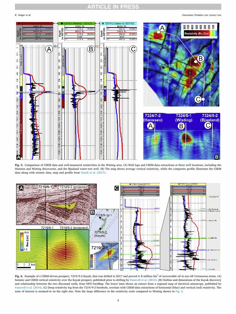
Fig. 5. Comparison of CSEM data and well-measured resistivities in the Wisting area. (A) Well logs and CSEM-data extractions at three well locations, including theHanssen and Wisting discoveries, and the Bjaaland water-wet well. (B) The map shows average vertical resistivity, while the composite profile illustrates the CSEMdata along with seismic data, map and profile from Granli et al. (2017).

Fig. 6. Example of a CSEM-driven prospect, 7219/9-2 Kayak, that was drilled in 2017 and proved 4–8 million Sm3 of recoverable oil in syn-rift Cretaceous strata. (A)Seismic and CSEM vertical resistivity over the Kayak prospect, published prior to drilling by Fanavoll et al. (2014). (B) Outline and dimensions of the Kayak discoveryand relationship between the two discussed wells, from NPD FactMap. The lower inset shows an extract from a regional map of electrical anisotropy, published byFanavoll et al. (2014). (C) Deep resistivity log from the 7219/9-2 borehole, overlain with CSEM-data extractions of horizontal (blue) and vertical (red) resistivity. Thezone of interest is zoomed-in on the right size. Note the large difference in the resistivity scale compared to Wisting shown in Fig. 5.

K. Senger et al. Geoscience Frontiers xxx (xxxx) xxx

8

Fig. 7. Resistivity variation in the different electro-facies grouped well by well. Overview of the horizontal resistivity measured in selected hydrocarbon-bearing wellsin the Barents Sea, subdivided into electro-facies representing the overburden, the organic-rich Hekkingen Formation cap rock and the gas and oil zones. The box-whisker plots provide a quick overview of the statistical distribution of the measured resistivity in each interval, plotting maximum, minimum, mean and theupper and lower quartiles.

K. Senger et al. Geoscience Frontiers xxx (xxxx) xxx

very convincing trend towards low velocity, high resistivity, high gammaray and high TOC source rock populations (Fig. 13).

5. Discussion

5.1. Resistivity controls in reservoir sandstones

The hydrocarbon bearing zones, subdivided into gas and oil zonesbased on the reported fluid contacts (Fig. 4), show the largest variation inresistivity spanning several orders of magnitude from 0.3 to>20 000Ωm(Fig. 7; Table 1). This is controlled primarily by reservoir quality andwater saturation. Since Archie (1942) proposed an empirical relationshiplinking porosity, water saturation and cementation, countless

9

publications have used or developed Archie’s law to quantify the watersaturation in the pay zone (e.g., Worthington, 1993 and referencestherein). This was motivated to quantify water saturation inlow-resistivity pay zones (Worthington, 2000), which can easily beoverlooked when only traditional water saturation estimates areattempted. A wide range of factors affecting pay zone resistivity existsthat includes shale content (Revil et al., 1998; Worthington, 1982), porethroat radius (Ziarani and Aguilera, 2012), cementation (Salem andChilingarian, 1999), temperature (Sen and Goode, 1992), salinity(Cameron et al., 1981; Worthington, 1993) and the presence of electri-cally conductive minerals such as pyrite or graphite (Pridmore andShuey, 1976; Spacapan et al., 2019). Rock physics work using electricalmeasurements is vastly under-represented in the literature when

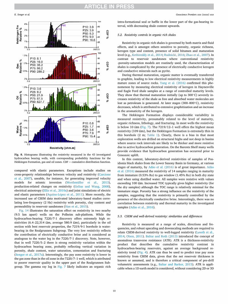
Fig. 8. Histograms illustrating the resistivity measured in the 43 investigatedhydrocarbon bearing wells, with corresponding probability functions for theHekkingen Formation, gas and oil zones. CDF ¼ cumulative distribution function.

K. Senger et al. Geoscience Frontiers xxx (xxxx) xxx

compared with elastic parameters. Exceptions include studies oncross-property relationships between velocity and resistivity (Carcioneet al., 2007), useable, for instance, for generating improved velocitymodels for seismic inversion (Werthmüller et al., 2013),production-related changes on resistivity (Gelius and Wang, 2008),electrical anisotropy (Ellis et al., 2010a) and joint simulations of electricand elastic parameters (Aquino-L�opez et al., 2011). More recently, theincreased use of CSEM data motivated laboratory-based studies corre-lating low-frequency (2 Hz) resistivity with porosity, clay content andpermeability in reservoir sandstones (Han et al., 2015).

Fig. 14 illustrates the saturation effect on resistivity in two nearby(9.5 km apart) wells on the Polheim sub-platform. While thehydrocarbon-bearing 7220/7-1 discovery offers extremely high re-sistivities (6.4–22,314 Ωm, average 580.9 Ωm), particularly in the oilsection with best reservoir properties, the 7219/9-1 borehole is water-bearing in the Realgrunnen Subgroup. The very low resistivity reflectsthe contribution of electrically conductive brine and is considered asanalogous to the water leg in the 7220/7-1 discovery. Note, however,that in well 7220/5–2 there is strong resistivity variation within thehydrocarbon bearing zone, probably reflecting vertical variation inporosity, shale content, water saturation, cementation and fracturing(Senger et al., 2017a). Interestingly, the pay zone resistivity is lower inthe gas zone than in the oil zone in the 7220/7–1well, which is attributedto poorer reservoir quality in the upper part of the Realgrunnen Sub-group. The gamma ray log in Fig. 7 likely indicates an organic rich

10

intra-formational seal or baffle in the lower part of the gas-bearing in-terval, with decreasing shale content upwards.

5.2. Resistivity controls in organic rich shales

Resistivity in organic rich shales is governed by both matrix and fluideffects, and is amongst others sensitive to porosity, organic richness,kerogen type and content, presence of solid bitumen and maturationlevel (e.g., Kethireddy et al., 2014; Rudnicki, 2016; Zhao et al., 2007). Incontrast to reservoir sandstones where conventional resistivity-porosity-saturation models are routinely used, the characterization ofshales is complicated by the presence of electrically conductive kerogenand conductive minerals such as pyrite.

During thermal maturation, organic matter is eventually transferredto graphite, leading to low electrical resistivity measurements in highlymature zones of source rocks. Yang et al. (2016) confirmed this phe-nomenon by measuring electrical resistivity of kerogen in Haynesvilleand Eagle Ford shale samples at a range of controlled maturity levels.They show that thermal maturation initially (up to 300�C) severely in-creases resistivity of the shale as free and absorbed water molecules arelost as petroleum is generated. At later stages (300–800�C), resistivitydecreases, which is attributed to extensive graphitization and an increasein the aromaticity of the kerogen.

The Hekkingen Formation displays considerable variability inmeasured resistivity, presumably related to the level of maturity,organic richness, lithology, and fracturing. In most wells the resistivityis below 10 Ωm (Fig. 7). The 7219/12–1 well offers the highest meanresistivity (109 Ωm), but the Hekkingen Formation is extremely thin inthis borehole (2 m; Table 1). Clearly, there is a bias in that mostexploration wells are drilled on structural highs and not deep in basinswhere source rock intervals are likely to be thicker and more resistivedue to active hydrocarbon generation. On the Barents Shelf many wellsprovide evidence that hydrocarbon generation has occurred prior toCenozoic uplift.

In this context, laboratory-derived resistivities of samples of Pos-idonia black shales from the Lower Saxony Basin in Germany, at variousstages of maturity, by Ad~ao et al. (2016) is of great importance. Ad~aoet al. (2016) measured the resistivity of 14 samples ranging in maturityfrom immature (0.53% Ro) to gas window (1.45% Ro) in both dry stateand when using distilled water. All samples were resistive with valuesexceeding 100 Ωm. Increased TOC typically gives higher resistivity (forthe dry samples) although the TOC range is relatively minimal for theimmature stage. Porosity has a strong influence on the resistivity of thesamples, suggesting that the resistivity is primarily controlled by thepresence of the electrically conductive brine. Interestingly, there was nocorrelation between resistivity and thermal maturity in the investigatedsamples (Ad~ao et al., 2016).

5.3. CSEM and well-derived resistivity: similarities and differences

Resistivity is measured at a range of scales, directions and fre-quencies, and robust upscaling and downscaling methods are required torelate CSEM-derived resistivity to well-logged resistivity (Løseth et al.,2014; Olsen, 2011). Baltar and Roth (2013) introduced the concept ofanomalous transverse resistance (ATR). ATR is a thickness-resistivityproduct that describes the cumulative resistivity contrast inhydrocarbon-bearing reservoirs, against an average background re-sistivity trend (Fig. 4). ATR can thus be used to predict true pay zoneresistivity from CSEM data, given that the net reservoir thickness isknown or assumed, and is therefore a critical component of pre-drillvolumetric assessments (e.g., Baltar and Barker, 2015). ATR is appli-cable when a 1D earthmodel is considered, without considering 2D or 3D

Fig. 9. Well correlation across selected wells showing vitrinite reflectance and Tmax with gamma ray and resistivity logs. The correlation also illustrates the thicknessvariation of the Hekkingen Formation (black part of discrete log). The oil window maturity ranges are 0.5–1.0 (Ro) and 435–455 �C (Tmax).

Fig. 10. Comparison of resistivity measured in boreholes with source rock maturity, as provided by vitrinite reflectance (VR, %Ro) and Tmax measurements on theHekkingen Formation. The data are plotted in both present-day depth, and in corrected depth reflecting the variable net erosion across the Barents Shelf. Thecorrection net erosion factors are listed in Table 1, and are based on a number of published erosion maps (Henriksen et al., 2011; Baig et al., 2016; Amantov andFjeldskaar, 2017; Ktenas et al., 2017; Lasabuda et al., 2018).

K. Senger et al. Geoscience Frontiers xxx (xxxx) xxx

effects. In the context of stacked reservoirs, or hydrocarbon-bearingsandstones overlain by resistive organic rich shales, the ATR equiva-lence principle can be applied to quantify the relative contribution of thetwo resistors. In addition, resistivity is a highly anisotropic and

11

scale-dependent parameter, with electrical conduction varying signifi-cantly with the direction and scale of the measurement. Electricalanisotropy is defined as Rv/Rh, where Rv ¼ vertical resistivity and Rh ¼horizontal resistivity. Electrical anisotropy is measurable at core

Fig. 11. Correlation between resistivity logs and vitrinite reflectance (VR) inthe Hekkingen Formation, color-coded by wells.

Fig. 12. Resistivity-sonic overlay of the 7219/8-1 S

K. Senger et al. Geoscience Frontiers xxx (xxxx) xxx

12

plug-scale in the lab (North et al., 2013; North and Best, 2014), towell-scale (Ellis et al., 2010a, 2010b; Moran and Gianzero, 1979) toCSEM-scale (Løseth et al., 2014; Newman et al., 2010). Modern 3D CSEMinversion is anisotropic, while most vertical exploration boreholes areprimarily sensitive to horizontal resistivity. Boreholes equipped withtri-axial resistivity tools able to derive the vertical resistivity are rare(e.g., Clavaud, 2008), particularly in non-reservoir sections. Nonetheless,several wells in the Barents Sea have acquired tri-axial data in theoverburden section (Vereshagin et al., 2019). This has been performedpartly to assist in interpreting CSEM data (Løseth et al., 2014) and toconstrain the effects of electrical anisotropy in the Barents Sea (Ellis et al.,2017; Schneider et al., 2015; Vereshagin et al., 2019; Wedberg et al.,2017). The scale of measurement also controls anisotropy; thereforeanisotropy at well-scale cannot be compared to anisotropy at CSEM-scale.Scaling effects from well to CSEM-scale must also be considered toaccurately represent small-scale variability at the well scale on thecoarser CSEM-scale (Olsen, 2011).

5.4. Implications for CSEM interpretation: applicability and limitations

Our objective is to quantify the resistivity variation within the Hek-kingen Formation compared to the underlying hydrocarbon-bearingreservoirs of the Realgrunnen Subgroup in the context of CSEM inter-pretation. As such, it is necessary to consider the transverse resistance

borehole. Rbaseline ¼ 2 Ωm, Δtbaseline ¼ 80 us/ft.

Fig. 13. Resistivity variation in the organic rich shales of the Hekkingen For-mation. (A) Resistivity versus sonic of the Hekkingen Formation, color-coded byTOC content measured in cuttings. (B) Cross-plot of resistivity vs. gamma ray,color-coded by TOC content measured in cuttings. Only wells where TOC data ismeasured in drill cores or cuttings are used, namely 7120/1–2.7120/12–1,7122/2–1, 7219/8-1 S, 7321/9–1, 7124/3–1, 7120/2-2, 7226/11–1, 7324/7-1S and DH5R.

Fig. 14. Well correlation across a hydrocarbon-bearing well 7220/7–1 and awater-bearing well 7219/9–1, flattened on top reservoir.

K. Senger et al. Geoscience Frontiers xxx (xxxx) xxx

(TR) of the different units as illustrated in Fig. 15 and listed in Table 1.The Hekkingen Formation typically exhibits TR values from 100 to 1000Ωm2, while the hydrocarbon-bearing zones usually exceed 1000Ωm2, insome cases by two orders of magnitude. With comparable zone thick-nesses of the hydrocarbon columns and Hekkingen Formation thicknessit is primarily the average zone resistivity that determines the TR of theunits.

As with other geophysical methods, CSEM has its limitations anduncertainties that must be evaluated to prevent interpretation pitfalls.Most importantly, CSEM data image subsurface resistivity. Thus, it is theresponsibility of the explorationists to evaluate the significance of anyenhanced subsurface resistivity with respect to possible hydrocarbons, orother resistivity-enhancing features. Integration with other data, inparticular seismic, is crucial for the interpretation of CSEM data (e.g.,Fanavoll et al., 2014; Tharimela et al., 2019). In addition, the interpretersmust be aware that there is some uncertainty in the vertical placement ofCSEM anomalies, which can be quantified through scenario testing usingCSEM forward modelling. On the other hand, the lateral placement ofCSEM anomalies is very good when 3D CSEM data are used, and can beused, for instance, to predict fluid contacts prior to drilling (Granli et al.,2017). Finally, geological complexity and increasing depth decrease the

13

CSEM sensitivity, which must be accounted for when interpreting CSEMdata.

Fig. 16 illustrates the CSEM response from five hydrocarbon-bearingdiscoveries and two water-bearing wells, all targeting the RealgrunnenSubgroup reservoir. The two water-bearing wells, 7324/2-1 Apollo and7324/8-2 Bjaaland, are both located near Wisting, where the targetreservoir is extremely shallow (200–250 m beneath the seafloor). From aCSEM-perspective, these shallow targets have extremely high sensitivity.Therefore, the lack of CSEM anomalies in both of these structures wasattributed to water-bearing, residual or low-saturation hydrocarbon-bearing reservoirs prior to drilling. The resistivity log from the drilledwells confirms the CSEM predictions, with conductive brine-bearingreservoirs. The high background resistivity may “hide” some low-tomoderate-saturation reservoirs, but it is notable that even minor hydro-carbon accumulations are imaged by CSEM data in the area. A goodexample of this is the 7325/4–1 Gemini gas discovery, located north-eastof Wisting, which demonstrates a strong CSEM anomaly corresponding toincreased resistivity within a 19 m thick gas column in the RealgrunnenSubgroup (Fig. 16). The operator reports 0.4 to 1 billion Sm3 of recov-erable gas, stating also that the discovery is not profitable as of today. Inother words, within this area of very high CSEM sensitivity, CSEM datacan detect even small gas accumulations below 1 billion Sm3, suggestingthat CSEM data should be considered as a tool for de-risking. Thestrength of the CSEM anomaly increases with both pay zone resistivityand pay zone thickness, well exemplified by the 7324/7-2 Hanssen and7324/8-1 Wisting wells (Figs. 5 and 16).

Further south in the Barents Sea, the Realgrunnen Subgroup is locateddeeper, at 900–1400 m below seafloor. Well log resistivity and reportedfluid contacts indicate a thicker pay zone in both the 7220/8-1 Skrugardand 7220/7-1 Havis discovery wells (both now part of Johan Castbergfield development). The extracted CSEM anomalies are not as strong as in

Fig. 15. Average resistivity versus zone thickness, color-coded by fluid phase in Realgrunnen Subgroup and the Hekkingen Fm. The transverse resistance (TR) linesillustrate the theoretical equal sensitivity of CSEM data to a resistor’s thickness�resistivity product. Table 1 provides details on the input data.

K. Senger et al. Geoscience Frontiers xxx (xxxx) xxx

the ultra-shallow reservoirs around Wisting. Here, increased sub-seabeddepth to reservoir interval results in a decrease in CSEM sensitivity.Nonetheless, both wells (7220/7-1 Havis in particular) exhibit con-strained vertical resistivity anomalies. Their lateral extent has beenpreviously shown to be constrained, and in agreement with theseismically-mapped structures (Fanavoll et al., 2014; Gabrielsen et al.,2013).

6. Conclusions

In this contribution we have investigated the resistivity variation asmeasured in exploration boreholes in the Barents Shelf, focusing on theresistivity variation in reservoir sandstones and the overlying cap rockshales. We conclude that:

(1) Resistivity in organic rich shales, in particular the Upper Juras-sic–Lower Cretaceous Hekkingen Formation source rock, is afunction of both the total organic content and its maturation stage.In the investigated wells, mean resistivity in the Hekkingen For-mation does not exceed 109 Ωm.

(2) The hydrocarbon bearing Realgrunnen Subgroup sandstonesexhibit extremely high resistivity in excess of several hundred tothousands Ωm. This is especially valid in fields and discoveriescurrently considered as commercial. In smaller discoveries where

14

development is considered unlikely (i.e. sub-commercial), the payzone resistivity is often less than 100 Ωm.

(3) We have particularly focused on parameters relevant for explo-ration away from well control where factors such as a resistor’stransverse resistance (i.e., thickness X resistivity), its sub-seafloordepth and vertical separation to other resistors are all importantwhen interpreting controlled-source electromagnetic data. Assuch, this study presents a framework for interpreting resistivitydata away from wells, such as CSEM or MT data sets.

(4) In organic rich shales, resistivity generally increases withincreasing maturity towards a depth-dependent threshold, fromwhich it decreases again towards over-mature source rocks.

(5) CSEM data are in very good agreement with resistivity measuredin wellbores, particularly in areas of high CSEM sensitivity such asthe shallow Realgrunnen Subgroup reservoirs in the northern partof the Barents Shelf.

(6) The transverse resistance of the encountered Hekkingen Forma-tion shales is found to be below 1000 Ωm2 in all wells. In contrast,transverse resistance in hydrocarbon-bearing reservoirs withinthe Realgrunnen Subgroup in most cases exceeds the 1000 Ωm2

threshold.

Declaration of competing interest

The authors declare that they have no known competing financial

Fig. 16. Overview of the resistivity response from borehole measurements and CSEM data for two water-bearing wells and five hydrocarbon-bearing wells. The wellcorrelation panel is flattened on the top of the Realgrunnen Subgroup reservoir, targeted by all wells. The reported volumes are from NPD (2019).

K. Senger et al. Geoscience Frontiers xxx (xxxx) xxx

interests or personal relationships that could have appeared to influencethe work reported in this paper.

Acknowledgements

This research is funded by the Research Centre for Arctic PetroleumExploration, supported by industry partners and the Research Council ofNorway (Grant No. 228107). PB was partly financed by the NorwegianCCS Centre, financed by the Research Council of Norway (Grant No.257579) and industry partners. We sincerely appreciate the generousdata access, particularly from the Norwegian Petroleum Directorate(DISKOS database, NPD FactPages and Svalbard exploration boreholes)and the UNIS CO2 lab (http://co2-ccs.unis.no) for access to the CO2

research boreholes onshore Svalbard. EMGS kindly provided CSEM dataat eight well locations. Amando Lasabuda kindly provided digital ver-sions of published net erosion maps. UNIS acknowledges the academiclicenses of Petrel and the Blueback Toolbox generously provided bySchlumberger and Cegal, respectively. Finally, we are grateful to twoanonymous journal reviewers for their constructive feedback, and GarethLord for proof-reading the manuscript.

References

Abay, T.B., Karlsen, D.A., Pedersen, J.H., Olaussen, S., Backer-Owe, K., 2018. Thermalmaturity, hydrocarbon potential and kerogen type of some Triassic–Lower Cretaceoussediments from the SW Barents Sea and Svalbard. Petrol. Geosci. 24 (3), 349–373.

Ad~ao, F., Ritter, O., Spangenberg, E., 2016. The electrical conductivity of Posidonia blackshales—from magnetotelluric exploration to rock samples. Geophys. Prospect. 64 (2),469–488.

15

Alvarez, P., Marcy, F., Vrijlandt, M., Skinnemoen, Ø., MacGregor, L., Nichols, K.,Keirstead, R., Bolivar, F., Bouchrara, S., Smith, M., 2018. Multi-physicscharacterisation of reservoir prospects in the Hoop area of the Barents Sea.Interpretation 6, 1–51.

Amantov, A., Fjeldskaar, W., 2018. Meso-Cenozoic exhumation and relevant isostaticprocess: the Barents and Kara shelves. J. Geodyn. 118, 118–139.

Anell, I., Braathen, A., Olaussen, S., 2014. The triassic-early jurassic of the northernBarents shelf: a regional understanding of the longyearbyen CO2 reservoir. Norw. J.Geol. 94, 83–98.

Aquino-L�opez, A., Mousatov, A., Markov, M., 2011. Model of sand formations for jointsimulation of elastic moduli and electrical conductivity. J. Geophys. Eng. 8, 568–578.

Archie, G.E., 1942. The electrical resistivity log as an aid in determining some reservoircharacteristics. Petroleum Technology 1422, 54–62.

Baig, I., Faleide, J.I., Jahren, J., Mondol, N.H., 2016. Cenozoic exhumation on thesouthwestern Barents Shelf: estimates and uncertainties constrained from compactionand thermal maturity analyses. Mar. Petrol. Geol. 73, 105–130.

Baltar, D., Barker, N.D., 2015. Prospectivity evaluation with 3D CSEM. First Break 33,55–62.

Baltar, D., Roth, F., 2013. Reserves estimation methods for prospect evaluation with 3DCSEM data. First Break 31, 103–111.

Barker, N., Baltar, D., 2016. CSEM anomaly identification. First Break 34, 47–50.Birchall, T., Senger, K., Hornum, M., Olaussen, S., Braathen, A., 2020. Underpressure in

the northern Barents shelf: Causes and implications for hydrocarbon exploration.AAPG Bull. https://doi.org/10.1306/02272019146. http://archives.datapages.com/data/bulletns/aop/2020-07-20/aapgbltn19146aop.html.

Blixt, E.M., Storvoll, V., Olstad, R., 2017. A statistical sensitivity method forCSEM—implications for petroleum exploration in the Barents Sea. First Break 35,37–44.

Buland, A., Løseth, L.O., Becht, A., Roudot, M., Røsten, T., 2011. The value of CSEM datain exploration. First Break 29, 69–76.

Cameron, D., Read, D., Jong, E.D., Oosterveld, M., 1981. Mapping salinity using resistivityand electromagnetic inductive techniques. Can. J. Soil Sci. 61, 67–78.

Carcione, J., Ursin, B., Nordskag, J., 2007. Cross-property relations between electricalconductivity and the seismic velocity of rocks. Geophysics 72, E193–E204.

Carstens, H., 2018. An Important Discovery, p. Geo365. https://geo365.no/olje-og-gass/an-important-discovery/.

K. Senger et al. Geoscience Frontiers xxx (xxxx) xxx

Cartwright, J., Huuse, M., 2005. 3D seismic technology: the geological ‘Hubble’. BasinRes. 17, 1–20.

Cavanagh, A.J., Di Primio, R., Scheck-Wenderoth, M., Horsfield, B., 2006. Severity andtiming of cenozoic exhumation in the southwestern Barents Sea. J. Geol. Soc. 163,761–774.

Clavaud, J.-B., 2008. Intrinsic electrical anisotropy of shale: the effect of compaction.Petrophysics 49, 243–260.

Constable, S., 2010. Ten years of marine CSEM for hydrocarbon exploration. Geophysics75, 75A67–75A81.

Dimakis, P., Braathen, B.I., Faleide, J.I., Elverhøi, A., Gudlaugsson, S.T., 1998. Cenozoicerosion and the preglacial uplift of the Svalbard–Barents Sea region. Tectonophysics300, 311–327.

Duran, E.R., di Primio, R., Anka, Z., Stoddart, D., Horsfield, B., 2013. 3D-basin modellingof the Hammerfest Basin (southwestern Barents Sea): a quantitative assessment ofpetroleum generation, migration and leakage. Mar. Petrol. Geol. 45, 281–303.

Eidesmo, T., Ellingsrud, S., MacGregor, L.M., Constable, S., Sinha, M.C., Johansen, S.,Kong, F.N., Westerdahl, H., 2002. Sea Bed Logging (SBL), a new method for remoteand direct identification of hydrocarbon filled layers in deepwater areas. First Break20, 144–152.

Ellingsrud, S., Eidesmo, T., Johansen, S., Sinha, M., MacGregor, L., Constable, S., 2002.Remote sensing of hydrocarbon layers by seabed logging (SBL): results from a cruiseoffshore Angola. Lead. Edge 21, 972–982.

Ellis, M., MacGregor, L., Newton, P., Keirstead, R., Bouchrara, S., Zhou, Y., Tseng, H.,2017. Investigating electrical anisotropy drivers across the Barents Sea. In: 79thEAGE Conference and Exhibition 2017, 12-15 June, Paris, France.

Ellis, M., Sinha, M., Parr, R., 2010a. Role of fine-scale layering and grain alignment in theelectrical anisotropy of marine sediments. First Break 28, 49–57.

Ellis, M.H., Sinha, M.C., Minshull, T.A., Sothcott, J., Best, A.I., 2010b. An anisotropicmodel for the electrical resistivity of two-phase geologic materials. Geophysics 75,E161–E170.

Evans, R.L., 2007. Using CSEM techniques to map the shallow section of seafloor: fromthe coastline to the edges of the continental slopeShallow-section EM mapping.Geophysics 72, WA105–WA116.

Faleide, J.I., Solheim, A., Fiedler, A., Hjelstuen, B.O., Andersen, E.S., Vanneste, K., 1996.Late Cenozoic evolution of the western Barents Sea-Svalbard continental margin.Global Planet. Change 12, 53–74.

Faleide, J.I., Tsikalas, F., Breivik, A.J., Mjelde, R., Ritzmann, O., Engen, Ø., Wilson, J.,Eldholm, O., 2008. Structure and evolution of the continental margin off Norway andthe Barents Sea. Episodes 31, 82–91.

Faleide, J.I., Vågnes, E., Gudlaugsson, S.T., 1993. Late Mesozoic-Cenozoic evolution of thesouth-western Barents Sea in a regional rift-shear tectonic setting. Mar. Petrol. Geol.10, 186–214.

Fanavoll, S., Gabrielsen, P., Ellingsrud, S., 2014. CSEM as a tool for better explorationdecisions: case studies from the Barents Sea. Norwegian Continental Shelf.Interpretation 2, SH55–SH66.

Gabrielsen, P.T., Abrahamson, P., Panzner, M., Fanavoll, S., Ellingsrud, S., 2013.Exploring frontier areas using 2D seismic and 3D CSEM data, as exemplified by multi-client data over the Skrugard and Havis discoveries in the Barents Sea. First Break 31,63–71.

Gelius, L.-J., Wang, Z., 2008. Modelling production caused changes in conductivity for asiliciclastic reservoir: a differential effective medium approach. Geophys. Prospect.56, 677–691.

Glørstad-Clark, E., Faleide, J.I., Lundschien, B.A., Nystuen, J.P., 2010. Triassic seismicsequence stratigraphy and paleogeography of the western Barents Sea area. Mar.Petrol. Geol. 27, 1448–1475.

Goswami, B.K., Weitemeyer, K.A., Bünz, S., Minshull, T.A., Westbrook, G.K., Ker, S.,Sinha, M.C., 2017. Variations in pockmark composition at the Vestnesa Ridge:insights from marine controlled source electromagnetic and seismic data. G-cubed18, 1111–1125.

Granli, J.R., Veire, H.H., Gabrielsen, P., Morten, J.P., 2017. Maturing Broadband 3DCSEM for Improved Reservoir Property Prediction in the Realgrunnen Group atWisting, Barents Sea, SEG Technical Program Expanded Abstracts 2017. Society ofExploration Geophysicists, pp. 2205–2209.

Grogan, P., Østvedt-Ghazi, A.M., Larssen, G.B., Fotland, B., Nyberg, K., Dahlgren, S.,Eidvin, T., 1999. Structural elements and petroleum geology of the Norwegian sectorof the northern Barents Sea. Geological Society, London, Petroleum GeologyConference series 5, 247–259.

Grundvåg, S.-A., Marin, D., Kairanov, B., �Sliwi�nska, K., Nøhr-Hansen, H., Escalona, A.,Olaussen, S., 2017. The lower cretaceous succession of the northwestern Barentsshelf: onshore and offshore correlations. Mar. Petrol. Geol. 86, 834–857.

Han, D.-H., Batzle, M., 2002. Fizz water and low gas-saturated reservoirs. Lead. Edge 21,395–398.

Han, T., Best, A.I., Sothcott, J., North, L.J., MacGregor, L.M., 2015. Relationships amonglow frequency (2 Hz) electrical resistivity, porosity, clay content and permeability inreservoir sandstones. J. Appl. Geophys. 112, 279–289.

Henriksen, E., Bjørnseth, H.M., Hals, T.K., Heide, T., Kiryukhina, T., Kløvjan, O.S.,Larssen, G.B., Ryseth, A.E., Rønning, K., Sollid, K., Stoupakova, A., 2011a. Chapter 17Uplift and erosion of the greater Barents Sea: impact on prospectivity and petroleumsystems. In: Spencer, A.M., Embry, A.F., Gautier, D.L., Stoupakova, A.V., Sørensen, K.(Eds.), Arctic Petroleum Geology. The Geological Society, London, pp. 271–281.

Henriksen, E., Ryseth, A.E., Larssen, G.B., Heide, T., Rønning, K., Sollid, K.,Stoupakova, A.V., 2011b. Chapter 10 Tectonostratigraphy of the greater Barents Sea:implications for petroleum systems. In: Spencer, A.M., Embry, A.F., Gautier, D.L.,Stoupakova, A.V., Sørensen, K. (Eds.), Arctic Petroleum Geology. The GeologicalSociety, London, pp. 163–195.

16

Hesthammer, J., Stefatos, A., Boulaenko, M., Fanavoll, S., Danielsen, J., 2010. CSEMperformance in light of well results. Lead. Edge 29, 34–41.

Høy, T., Lundschien, B.A., 2011. Chapter 15 triassic deltaic sequences in the northernBarents Sea. In: Spencer, A.M., Embry, A.F., Gautier, D.L., Stoupakova, A.V.,Sørensen, K. (Eds.), Arctic Petroleum Geology. Geological Society, Memoir #35,London, pp. 249–260.

Jakobsson, K., 2018. A history of exploration offshore Norway: the Barents Sea.Geological Society, London, Special Publications 465. SP465. 418.

Johansen, S., Gabrielsen, P., 2015. Interpretation of marine CSEM and marine MT data forhydrocarbon prospecting. In: Bjørlykke, K. (Ed.), Petroleum Geoscience. SpringerBerlin Heidelberg, pp. 515–544.

Johansen, S.E., Panzner, M., Mittet, R., Amundsen, H.E., Lim, A., Vik, E., Landrø, M.,Arntsen, B., 2019. Deep electrical imaging of the ultraslow-spreading Mohns Ridge.Nature 567, 379.

Johnson, H.M., 1962. A history of well logging. Geophysics 27, 507–527.Kethireddy, N., Chen, H., Heidari, Z., 2014. Quantifying the effect of kerogen on

resistivity measurements in organic-rich mudrocks. Petrophysics 55, 136–146.Klausen, T.G., Müller, R., Poyatos-Mor�e, M., Olaussen, S., Stueland, E., 2019a. Tectonic,

provenance and sedimentological controls on reservoir characteristics in the uppertriassic–middle jurassic realgrunnen Subgroup, SW Barents Sea. Geological Society,London, Special Publications 495. SP495-2018-2165.

Klausen, T.G., Müller, R., Slama, J., Helland-Hansen, W., 2017. Evidence for late triassicprovenance areas and early jurassic sediment supply turnover in the Barents Seabasin of northern pangea. Lithosphere 9, 14–28.

Klausen, T.G., Nyberg, B., Helland-Hansen, W., 2019c. The largest delta plain in Earth’shistory. Geology 47, 470–474.

Koevoets, M.J., Hammer, Ø., Olaussen, S., Senger, K., Smelror, M., 2019. Integratingsubsurface and outcrop data of the Middle jurassic to lower cretaceous agardfjelletFormation in central spitsbergen. Norw. J. Geol. 98, 1–34.

Ktenas, D., Henriksen, E., Meisingset, I., Nielsen, J.K., Andreassen, K., 2017.Quantification of the magnitude of net erosion in the southwest Barents Sea usingsonic velocities and compaction trends in shales and sandstones. Mar. Petrol. Geol.88, 826–844.

Lasabuda, A., Geissler, W.H., Laberg, J.S., Knutsen, S.M., Rydningen, T.A., Berglar, K.,2018. Late Cenozoic erosion estimates for the northern Barents Sea: quantifyingglacial sediment input to the Arctic Ocean. G-cubed 19, 4876–4903.

Lerch, B., Karlsen, D.A., Thieβen, O., Abay, T.B., van Soelen, E.E., Kürschner, W.M.,Planke, S., Backer-Owe, K., 2018. Investigations on the use of triaromaticdimethylcholesteroids as age-specific biomarkers in bitumens and oils from ArcticNorway. Org. Geochem. 122, 1–16.

Lundschien, B.A., Høy, T., Mørk, A., 2014. Triassic hydrocarbon potential in the NorthernBarents Sea; integrating Svalbard and stratigraphic core data. Norwegian PetroleumDirectorate Bulletin 11, 3–20.

Løseth, L.O., Wiik, T., Olsen, P.A., Hansen, J.O., 2014. Detecting Skrugard by CSEM —

prewell prediction and postwell evaluation. Interpretation 2 (3), SH67–SH78.MacGregor, L., 2012. Integrating seismic, CSEM, and well-log data for reservoir

characterization. Lead. Edge 268–277.MacGregor, L., Bouchrara, S., Tomlinson, J., Strecker, U., Fan, J., Ran, X., Yu, G., 2012.

Integrated analysis of CSEM, seismic and well log data for prospect appraisal: a casestudy from West Africa. First Break 30, 43–48.

MacGregor, L., Tomlinson, J., 2014. Marine controlled-source electromagnetic methodsin the hydrocarbon industry: a tutorial on method and practice. Interpretation 2,SH13–SH32.

Matapour, Z., Karlsen, D., Lerch, B., Backer-Owe, K., 2019. Petroleum occurrences in thecarbonate lithologies of the Gohta and Alta discoveries in the Barents Sea, arcticNorway. Petrol. Geosci. 25, 50–70.

McCarthy, K., Rojas, K., Niemann, M., Palmowski, D., Peters, K., Stankiewicz, A., 2011.Basin petroleum geochemistry for source rock evaluation. Oilfield Rev. 23, 32–43.

Midtkandal, I., Faleide, J.I., Faleide, T.S., Serck, C.S., Planke, S., Corseri, R., Dimitriou, M.,Nystuen, J.P., 2020. Lower Cretaceous Barents Sea strata: epicontinental basinconfiguration, timing, correlation and depositional dynamics. Geol. Mag. 157 (3),458–476.

Moran, J., Gianzero, S., 1979. Effects of formation anisotropy on resistivity-loggingmeasurements. Geophysics 44, 1266–1286.

Mulrooney, M.J., Leutscher, J., Braathen, A., 2017. A 3D structural analysis of the Goliatfield, Barents Sea, Norway. Mar. Petrol. Geol. 86, 192–212.

Müller, R., Klausen, T., Faleide, J., Olaussen, S., Eide, C., Suslova, A., 2019. Linkingregional unconformities in the Barents Sea to compression-induced forebulge uplift atthe Triassic-Jurassic transition. Tectonophysics 765, 35–51.

Mørk, M.B.E., 2013. Diagenesis and quartz cement distribution of low-permeability UpperTriassic –Middle Jurassic reservoir sandstones, Longyearbyen CO2 lab well site inSvalbard, Norway. AAPG (Am. Assoc. Pet. Geol.) Bull. 97, 577–596.

Newman, G., Commer, M., Carazzone, J., 2010. Imaging CSEM data in the presence ofelectrical anisotropy. Geophysics 75, F51–F61.

North, L., Best, A.I., Sothcott, J., MacGregor, L., 2013. Laboratory determination of thefull electrical resistivity tensor of heterogeneous carbonate rocks at elevatedpressures. Geophys. Prospect. 61, 458–470.

North, L.J., Best, A.I., 2014. Anomalous electrical resistivity anisotropy in clean reservoirsandstones. Geophys. Prospect. 62, 1315–1326.

NPD, 2015. Resource accounts for the Norwegian continental shelf as of 31 December2015. http://www.npd.no/en/Topics/Resource-accounts-and–analysis/Temaartikler/Resource-accounts/2015/.

NPD, 2019. FactPages accessed 01.08.2019.Nøttvedt, A., Livbjerg, F., Midbøe, P.S., Rasmussen, E., 1993. Hydrocarbon potential of

the central spitsbergen basin. In: Vorren, T.O., Bergsager, E., Dahl-Stamnes, Ø.A.,

K. Senger et al. Geoscience Frontiers xxx (xxxx) xxx

Holter, E., Johansen, B., Lie, E., Lund, T.B. (Eds.), Arctic Geology and PetroleumPotential. Elsevier, Amsterdam, pp. 333–361.

Ohm, S.E., Karlsen, D.A., Austin, T.J.F., 2008. Geochemically driven exploration modelsin uplifted areas: examples from the Norwegian Barents Sea. AAPG (Am. Assoc. Pet.Geol.) Bull. 92, 1191–1223.

Olaussen, S., Larssen, G., Helland-Hansen, W., Johannessen, E., Nøttvedt, A., Riis, F.,Rismyhr, B., Smelror, M., Worsley, D., 2018. Mesozoic strata of kong karls land,svalbard, Norway; a link to the northern Barents Sea basins and platforms. Norw. J.Geol. 98, 1–69. https://doi.org/10.17850/njg98-4-06.

Olsen, P.A., 2011. Coarse-scale resistivity for saturation estimation in heterogeneousreservoirs based on Archie’s formula. Geophysics 76, E35–E43.

OMV, 2019. Increased Wisting Volumes.Passey, Q., Creaney, S., Kulla, J., Moretti, F., Stroud, J., 1990. A practical model for

organic richness from porosity and resistivity logs. AAPG Bull. 74, 1777–1794.Pridmore, D., Shuey, R., 1976. The electrical resistivity of galena, pyrite, and

chalcopyrite. Am. Mineral. 61, 248–259.Revil, A., Cathles, L.M., Losh, S., Nunn, J.A., 1998. Electrical conductivity in shaly sands

with geophysical applications. J. Geophys. Res.: Solid Earth 103, 23925–23936.Rossi, V.M., Olaussen, S., Staine, I.N., Gennaro, M., 2020. Development of the Middle

triassic kobbe Formation shelf-margin prism and transgressive-regressive cycles onthe shelf (Hammerfest Basin, SW Barents Sea). Mar. Petrol. Geol. 111, 868–885.

Rudnicki, M.D., 2016. Variation of organic matter density with thermal maturity. AAPG(Am. Assoc. Pet. Geol.) Bull. 100, 17–22.

Ryseth, A., 2014. Sedimentation at the jurassic–triassic boundary, south-west Barents Sea.In: From Depositional Systems to Sedimentary Successions on the NorwegianContinental Margin. John Wiley & Sons, Ltd, pp. 187–214.

Rønnevik, H.C., 2015. Exploration strategy. In: Bjørlykke, K. (Ed.), Petroleum Geoscience.Springer, pp. 639–651.

Salem, H.S., Chilingarian, G.V., 1999. The cementation factor of Archie’s equation forshaly sandstone reservoirs. J. Petrol. Sci. Eng. 23, 83–93.

Schneider, R.V., Bouchrara*, S., MacGregor, L., Alvarez, A., Ellis, M., Ackermann, R.,Newton, P., Keirstead, R., Rusic, A., Zhou, Y., 2015. CSEM based anisotropy trends inthe Barents Sea. In: SEG Technical Program Expanded Abstracts 2015. Society ofExploration Geophysicists, pp. 879–883.

Schwalenberg, K., Rippe, D., Koch, S., Scholl, C., 2017. Marine-controlled sourceelectromagnetic study of methane seeps and gas hydrates at Opouawe Bank,Hikurangi Margin, New Zealand. J. Geophys. Res.: Solid Earth 122, 3334–3350.

Sen, P., Goode, P., 1992. Influence of temperature on electrical conductivity on shalysands. Geophysics 57, 89–96.

Senger, K., Birchall, T., Ohm, S., Ogata, K., Olaussen, S., 2017a. Review of geologicalcontrols on resistivity in uplifted basins: insights from the Norwegian Barents shelf.In: AAPG International Conference & Exhibition, London, UK, 15-18 October 2017,p. 10.

Senger, K., Brugmans, P., Grundvåg, S.-A., Jochmann, M., Nøttvedt, A., Olaussen, S.,Skotte, A., Smyrak-Sikora, A., 2019. Petroleum, coal and research drilling onshoreSvalbard: a historical perspective. Norw. J. Geol. 99 (3), 1–30.

Senger, K., Millett, J., Planke, S., Ogata, K., Eide, C., Festøy, M., Galland, O., Jerram, D.,2017b. Effects of igneous intrusions on the petroleum system: a review. First Break35, 10.

Senger, K., Svendsen, R., Gabrielsen, P., Fanavoll, S., Pedersen, C.B., Kjølhamar, B., 2015.Regional Resistivity Trends in the Northern Barents Sea: Insights from CSEM Data.Norsk Geologisk Vinterkonferansen 12-14.1.2015, Stavanger, Norway.

17

Senger, K., Tveranger, J., Ogata, K., Braathen, A., Planke, S., 2014. Late mesozoicmagmatism in svalbard: a review. Earth Sci. Rev. 139, 123–144.

Serck, C.S., Faleide, J.I., Braathen, A., Kjølhamar, B., Escalona, A., 2017. Jurassic to earlycretaceous basin configuration (s) in the fingerdjupet subbasin, SW Barents Sea. Mar.Petrol. Geol. 86, 874–891.

Shephard, G.E., Müller, R.D., Seton, M., 2013. The tectonic evolution of the Arctic sincePangea breakup: integrating constraints from surface geology and geophysics withmantle structure. Earth Sci. Rev. 124, 148–183.

Spacapan, J.B., D’Odorico, A., Palma, O., Galland, O., Senger, K., Ruiz, R., Manceda, R.,Leanza, H.A., 2019. Low resistivity zones at contacts of igneous intrusions emplacedin organic-rich formations and their implications on fluid flow and petroleumsystems: a case study in the northern Neuqu�en Basin, Argentina. Basin Res. 32, 3–24.

Steel, R.J., Worsley, D., 1984. Svalbard’s post-Caledonian strata - an atlas ofsedimentational patterns and paleogeographic evolution. In: Spencer, A.M. (Ed.),Petroleum Geology of the North European Margin. Graham & Trotman, London,pp. 109–135.

Stefatos, A., Vereshagin, A., Hesthammer, J., Kalstø, T., Sperrevik, S., Robson, A., 2014.CSEM-driven exploration over the nordland ridge. Interpretation 2, SH79–SH95.

Tharimela, R., Augustin, A., Ketzer, M., Cupertino, J., Miller, D., Viana, A., Senger, K.,2019. 3D controlled-source electromagnetic imaging of gas hydrates: insights fromthe Pelotas Basin offshore Brazil. Interpretation 7, SH111–SH131.

Vereshagin, A., Wedberg, T., Stefatos, A., 2019. Predicting vertical resistivity by machinelearning. In: 81st EAGE Conference and Exhibition 2019. European Association ofGeoscientists & Engineers, pp. 1–5.

Wedberg, T., Stefatos, A., Vereshagin, A., 2017. Up scaling of triaxial resistivity datameasured on the Norwegian Continental Shelf and observations relevant for CSEMimaging. In: AAPG/SEG Conference and Exhibition. Search and Discovery Article#90310, London, England.

Weitemeyer, K.A., Constable, S., Tr�ehu, A.M., 2011. A marine electromagnetic survey todetect gas hydrate at Hydrate Ridge, Oregon. Geophys. J. Int. 187, 45–62.

Wennberg, O.P., Malm, O., Needham, T., Edwards, E., Ottesen, S., Karlsen, F., Rennan, L.,Knipe, R., 2008. On the occurrence and formation of open fractures in the Jurassicreservoir sandstones of the Snøhvit Field, SW Barents Sea. Petrol. Geosci. 14,139–150.

Werthmüller, D., Ziolkowski, A., Wright, D., 2013. Background resistivity model fromseismic velocities. Geophysics 78, E213–E223.

Worsley, D., 2008. The post-Caledonian development of Svalbard and the western BarentsSea. Polar Res. 27, 298–317.

Worthington, P.F., 1982. The influence of shale effects upon the electrical resistivity ofreservoir rocks. Geophys. Prospect. 30, 673–687.

Worthington, P.F., 1993. The uses and abuses of the Archie equations, 1: the formationfactor-porosity relationship. J. Appl. Geophys. 30, 215–228.

Worthington, P.F., 2000. Recognition and evaluation of low-resistivity pay. Petrol.Geosci. 6, 77–92.

Yang, A., Firdaus, G., Heidari, Z., 2016. Electrical resistivity and chemical properties ofkerogen isolated from organic-rich mudrocks. Geophysics 81, D643–D655.

Zhao, H., Givens, N.B., Curtis, B., 2007. Thermal maturity of the Barnett Shale determinedfrom well-log analysis. AAPG Bull. 91, 535–549.

Ziarani, A.S., Aguilera, R., 2012. Pore-throat radius and tortuosity estimation fromformation resistivity data for tight-gas sandstone reservoirs. J. Appl. Geophys. 83,65–73.

Zweidler, D., Baltar, D., Barker, N., 2015. Impact of CSEM on Return of ExplorationInvestment. Hart’s E&P.