Work supported by Department of Energy contract DE–AC02–76SF00515.

Stanford Linear Accelerator Center, Stanford University, Stanford, CA 94309

SLAC-R-783

Hosing Instability of the Drive Electron Beam in the E157Plasma-Wakefield Acceleration Experiment at the

Stanford Linear Accelerator

By Brent Edward Blue

UNIVERSITY OF CALIFORNIA

Los Angeles

Hosing Instability of the Drive Electron Beam in the

E157 Plasma-Wakefield Acceleration Experiment

at the Stanford Linear Accelerator

A thesis submitted in partial satisfaction

of the requirements for the degree Master of Science

in Electrical Engineering

by

Brent Edward Blue

2000

iii

Contents List of Figures iv Acknowledgements vi Abstract 1 Introduction 1

1.1 What is the PWFA? …………………………………………… 1 1.2 What is E157? …………………………………………………… 2 1.3 What is the Hosing Instability? …………………………………… 7 1.4 How Might One Look for the Hosing Instability? …………… 9

2 Theory of the Hosing Instability 11

2.1 Theory of the Hosing Instability – Offset Oscillations …………… 11 2.2 Theory of Hosing II …………………………………………… 14 2.3 Limitations to the Theory of Hosing …………………………… 21

3 Experimental Setup 23

3.1 Stanford Linear Accelerator (SLAC) …………………………… 24 3.2 Final Focus Test Beam (FFTB) …………………………………… 25 3.3 Lithium plasma source …………………………………………… 27 3.4 Optical Transition Radiators (OTR) …………………………… 28 3.5 Beam Position Monitors (BPMs) …………………………………… 32 3.6 Aerogel Cherenkov Radiator …………………………………… 33

4 Results 37 4.1 Initial Beam Condition …………………………………………… 37 4.2 Centroid Oscillations …………………………………………… 42 4.3 Tail Flipping …………………………………………………… 47 4.4 Tail Growth on Streak Camera Diagnostic …………………… 53 4.5 BPM Data for a High Density Run …………………………… 56

5 Conclusion 62 5.1 Summary …………………………………………………………… 62 5.2 Future Directions …………………………………………………… 62

Appendix A FFTB Beamline …………………………………………… 64 Appendix B Typical Electron Beam Parameters …………………………… 72 Bibliography …………………………………………………………………… 73

viii

iv

List of Figures 1.1.1 Cartoon of the electron beam displacing electrons and generating a plasma wave ……………………………………………………. 2 1.2.1 Energy vs. Year For High Energy Accelerators ……………………. 4 1.2.2 Schematic for the NLC with SLAC drawn for size comparison ……. 5 1.3.1 Cartoon of tilted beam before plasma (A), inside the plasma (B),

and after the plasma (C). The nomenclature for our tilted beam (A) is the head defines the axis and the centroid is displaced from the axis by ro. In the plasma, the head goes straight while the body oscillates. As the beam exists the plasma, the head continues straight while the body, with some perpendicular momentum, travels off at some angle. ……………………. 8

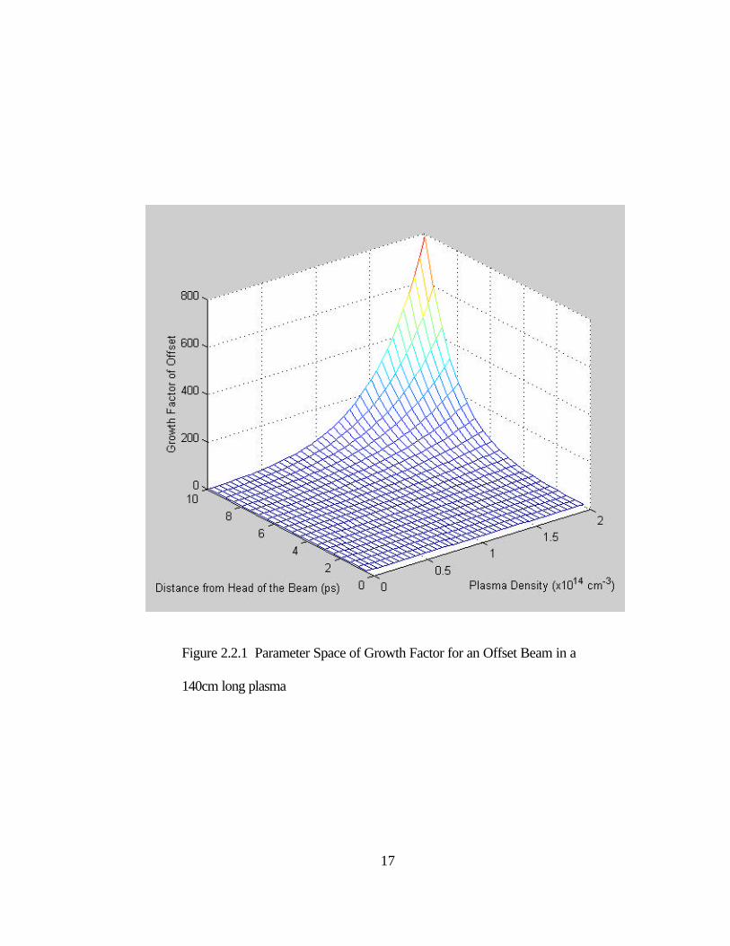
2.2.1 Parameter Space of Growth Factor for an Offset Beam in a 140cm long plasma ……………………………………………………. 17

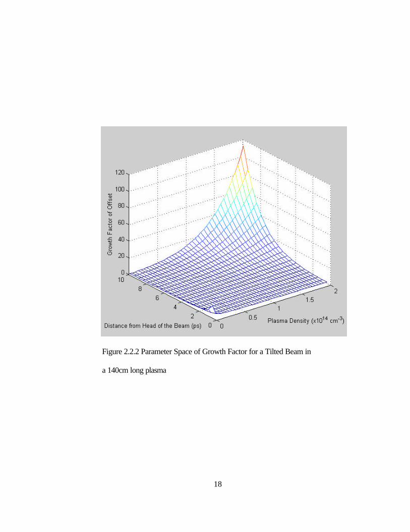
2.2.2 Parameter Space of Growth Factor for a Tilted Beam in a 140cm long plasma ……………………………………………………. 18

2.2.3 Oscillation of a tilted beam in a 2x1014 cm–3 plasma for a channel which is formed 2ps before the centroid ……………………. 19

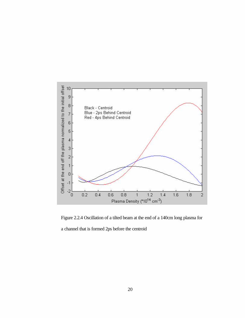
2.2.4 Oscillation of a tilted beam at the end of a 140cm long plasma for a channel which is formed 2ps before the centroid ……………………. 20

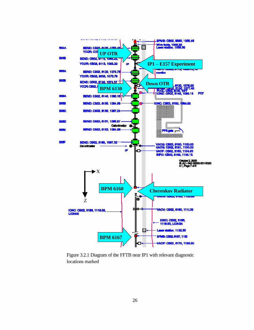
2.3.1 Dynamics of Ion Channel Formation ……………………………………. 22 3.0.1 Experimental Setup and Diagnostic Locations ……………………. 23 3.2.1 Diagram of the FFTB near IP1 with relevant diagnostic locations

marked ……………………………………………………………………. 26 3.3.1 Diagram of Lithium Oven Setup and Depiction of Lithium Column ……. 28 3.4.1 Upstream and Downstream OTR Images ……………………………. 30 3.4.2 Image analysis of upstream and downstream OTR images………………. 31 3.5.1 Typical Stripline BPM ……………………………………………. 32 3.6.1 Time Integrated Cherenkov Image depicting the parts of the beam

seen by the horizontal and vertical slits on the streak camera ……. 34 3.6.2 Typical Streak Camera image showing both the horizontal and

vertical streaks ……………………………………………………. 35 3.6.3 Diagram of Cherenkov radiation detector setup ……………………. 36 4.1.1 Streak Camera Data ……………………………………………………. 38 4.1.2 Tilted Beams ……………………………………………………………. 39 4.1.3 Average of 25 laser off shots ……………………………………………. 39

v

4.1.4 Fit to envelope equation ……………………………………………. 41 4.1.5 Scaling of Beam Tilt ……………………………………………………. 41 4.1.6 Centroid offset at plasma entrance ……………………………………. 42 4.2.1 Upstream OTR images showing tails in x-y plane ……………………. 43 4.2.2 Centroid Oscillations downstream from the plasma in both

the x and y planes ……………………………………………………. 43 4.2.3 Centroid Oscillations on downstream OTR ……………………………. 44 4.2.4 Betatron oscillations ……………………………………………………. 45 4.2.5 Single electron motion within the beam ……………………………. 46 4.3.1 Spot size data from the 3rd pinch showing the bins ……………………. 48 4.3.2 Spot size data from the 4th pinch showing the bins ……………………. 49 4.3.3 Justification of the 3rd pinch location ……………………………………. 50 4.3.4 Correspondence between horizontal and vertical pinch energy

at the 4th pinch ……………………………………………………………. 50 4.3.5 Tail motion at the 3rd pinch ……………………………………………. 51 4.3.6 Tail motion at the 4th pinch ……………………………………………. 52 4.4.1 Time slice analysis at laser off, second, and fourth pinch ……………. 54 4.4.2 Growth of normalized slice offsets vs. theoretical hosing curve ……. 55 4.5.1 Oscillations of beam centroid after plasma exit as measured

on downstream OTR and on BPMs 6130, 6160, 6167, and 6170 ……. 57 4.5.2 Beam trajectory exiting plasma ……………………………………. 58 4.5.3 Slope of the beams exit trajectory as a function of laser energy ……. 58 4.5.4 Plot of envelope equation (shown in blue) versus plasma density

superimposed on a plot of the beams spot size (red diamonds) versus incident UV laser energy. This fit is used to convert the incident UV laser energy into plasma density. ……………………. 59

4.5.5 Perpendicular Energy of Beam in a High Density Plasma ……………. 61

vi

Acknowledgements It has been a great pleasure to work in the fields of plasma physics at UCLA and USC

and the field of high-energy physics at Stanford. I would like to thank all of the

faculty, staff, and students that I have worked and collaborated with at these first-rate

institutions.

In particular I would like to first thank Dean Katsouleas for his support and guidance.

This work would not have been possible if it were not for the many long hours in the

E157 trailer Tom spent teaching me the dynamics of an electron beam in a plasma. I

would like to also thank Prof. Muggli for not only working on the E157 collaboration,

but also for his guidance on plasma physics in general.

I would like to also thank my colleagues at Stanford. Prof. Siemann has helped me

out considerably in the fields of high-energy physics. Special thanks needs to be given

for all of the Matlab code he has written which made my data analysis possible. I am

eternally grateful to all of the work Dr. Hogan has contributed to the E157 experiment.

If it were not for his work, none of my work would have been possible.

Special thanks need to be given to my colleagues at UCLA. Dr. Chris Clayton has

taught me about physics and opened my eyes on seeing problems in a whole new light.

vii

Ken Marsh deserves special credit for bringing me on to the E157 collaboration. I

would also like to thank Sho Wang for his “can-do-it” attitude and his support during

the many hours we spent working in the trailer.

Finally, I would like to thank Prof. Chan Joshi, my advisor, who has been working

with me on every detail of this research. If it were not for his guidance and support,

this thesis would not be possible.

viii

ABSTRACT OF THE THESIS

Hosing Instability of the Drive Electron Beam in the

E157 Plasma-Wakefield Acceleration Experiment

at the Stanford Linear Accelerator

by

Brent Edward Blue

Master of Science in Electrical Engineering

University of California, Los Angeles, 2000

Professor Chandrasekhar J. Joshi, Chair

In the plasma-wakefield experiment at SLAC, known as E157, an ultra-relativistic

electron beam is used to both excite and witness a plasma wave for advanced

accelerator applications. If the beam is tilted, then it will undergo transverse

oscillations inside of the plasma. These oscillations can grow exponentially via an

instability know as the electron hose instability. The linear theory of electron-hose

instability in a uniform ion column predicts that for the parameters of the E157

experiment (beam charge, bunch length, and plasma density) a growth of the centroid

offset should occur. Analysis of the E157 data has provided four critical results. The

ix

first was that the incoming beam did have a tilt. The tilt was much smaller than the

radius and was measured to be 5.3 µm/σz at the entrance of the plasma (IP1.) The

second was the beam centroid oscillates in the ion channel at half the frequency of the

beam radius (betatron beam oscillations), and these oscillations can be predicted by

the envelope equation. Third, up to the maximum operating plasma density of E157

(~2×1014 cm-3), no growth of the centroid offset was measured. Finally, time-resolved

data of the beam shows that up to this density, no significant growth of the tail of the

beam (up to 8ps from the centroid) occurred even though the beam had an initial tilt.

1

1 Introduction

1.1 What is the PWFA?

Plasma based accelerators are of great interest because of their potential to

accelerate charged particles at high gradients. Conventional radio frequency

accelerators are limited to approximately 100 MV/m. This limit is partly due to

breakdown in the walls of the structure. On the other hand, a plasma can sustain

electron plasma waves with electric fields on the order of the nonrelativistic wave

breaking field [1], ecmE peo /ω= , where 2/12 )/4( eop menπω = is the electron plasma

frequency and no is the electron plasma density. Since the electric field scales as the

square root of density, electric fields are on the order of 1-100 GV/m for plasma

densities in the range of 1014-1018 cm-3.

Plasma based accelerators utilize a laser or a charged particle beam to drive a

relativistically propagating plasma wave [2]. Laser driven accelerator schemes

include the beat-wave accelerator [3], the laser-wake field accelerator [4], and the self-

modulated wake field accelerator [5]. These schemes possess the ability to generate

high density plasma waves (~1018 cm-3), and therefore, high electric field gradients

(~100 GV/m.) The shortcoming of these schemes is that the length of the accelerator

is limited to a few Rayleigh lengths of the laser beam (< 1cm.) Charged particle

beam driven plasma wake field accelerators (PWFA) are capable of long interaction

2

lengths (on the order of meters), at the expense of a decreased accelerating gradient (~

10 – 1000 MV/m.)

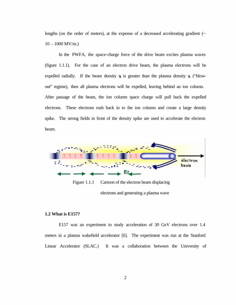
In the PWFA, the space-charge force of the drive beam excites plasma waves

(figure 1.1.1). For the case of an electron drive beam, the plasma electrons will be

expelled radially. If the beam density nb is greater than the plasma density no (“blow-

out” regime), then all plasma electrons will be expelled, leaving behind an ion column.

After passage of the beam, the ion column space charge will pull back the expelled

electrons. These electrons rush back in to the ion column and create a large density

spike. The strong fields in front of the density spike are used to accelerate the electron

beam.

Figure 1.1.1 Cartoon of the electron beam displacing

electrons and generating a plasma wave

1.2 What is E157?

E157 was an experiment to study acceleration of 30 GeV electrons over 1.4

meters in a plasma wakefield accelerator [6]. The experiment was run at the Stanford

Linear Accelerator (SLAC.) It was a collaboration between the University of

3

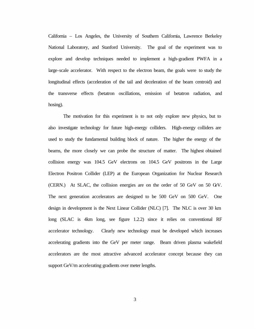
California – Los Angeles, the University of Southern California, Lawrence Berkeley

National Laboratory, and Stanford University. The goal of the experiment was to

explore and develop techniques needed to implement a high-gradient PWFA in a

large-scale accelerator. With respect to the electron beam, the goals were to study the

longitudinal effects (acceleration of the tail and deceleration of the beam centroid) and

the transverse effects (betatron oscillations, emission of betatron radiation, and

hosing).

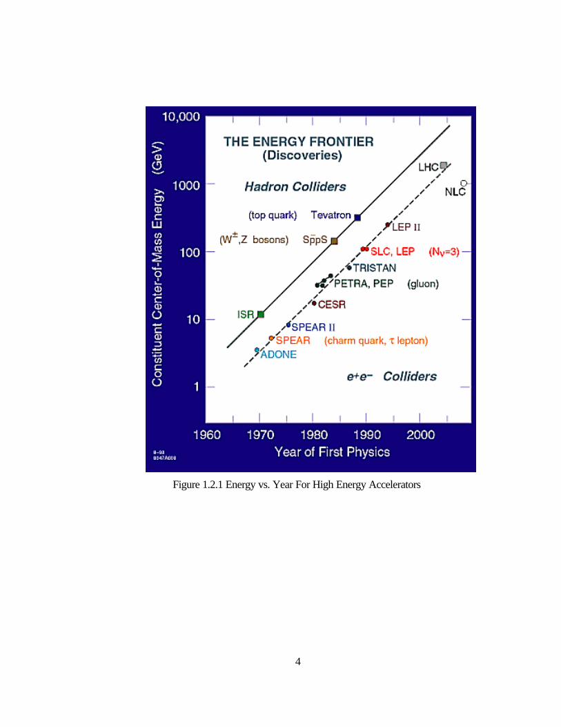
The motivation for this experiment is to not only explore new physics, but to

also investigate technology for future high-energy colliders. High-energy colliders are

used to study the fundamental building block of nature. The higher the energy of the

beams, the more closely we can probe the structure of matter. The highest obtained

collision energy was 104.5 GeV electrons on 104.5 GeV positrons in the Large

Electron Positron Collider (LEP) at the European Organization for Nuclear Research

(CERN.) At SLAC, the collision energies are on the order of 50 GeV on 50 GeV.

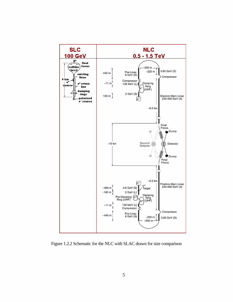
The next generation accelerators are designed to be 500 GeV on 500 GeV. One

design in development is the Next Linear Collider (NLC) [7]. The NLC is over 30 km

long (SLAC is 4km long, see figure 1.2.2) since it relies on conventional RF

accelerator technology. Clearly new technology must be developed which increases

accelerating gradients into the GeV per meter range. Beam driven plasma wakefield

accelerators are the most attractive advanced accelerator concept because they can

support GeV/m accelerating gradients over meter lengths.

4

Figure 1.2.1 Energy vs. Year For High Energy Accelerators

5

Figure 1.2.2 Schematic for the NLC with SLAC drawn for size comparison

6

The basic idea of the E157 experiment is to use a single electron bunch where

the front of the beam excites a plasma wave and the tail of the beam witnesses the

resulting accelerating field. The nominal beam parameters were 2x1010, 30 GeV

electrons, a bunch length of 0.7mm, and a transverse spot size of 40 µm. This beam

was propagated through a 1.4m long Lithium plasma of a density up to 2x1014 e-/cm-3.

The plasma source is positioned at interaction point 1 in the Final Focus Test Beam

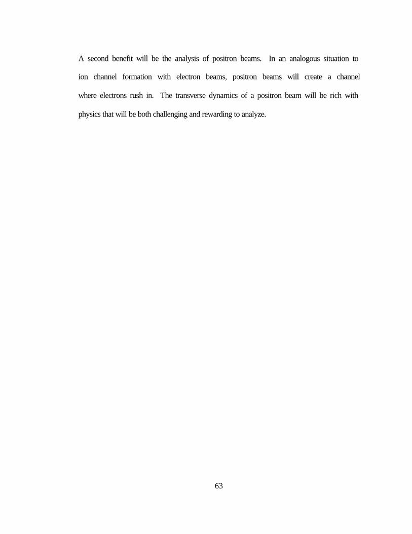
(FFTB) at SLAC. The FFTB is a straight shot down the 3km long accelerator and was

designed to investigate the factors that limit the size and stability of the beam at the

collision point of a linear collider. The importance of the FFTB design to our

experiment is that the beam optics and diagnostics are capable of delivering a high

quality beam to our experiment. In addition to the diagnostics built into the FFTP

(beam position monitors, current measuring torroids, and wire scanners), the

experiment required single shot beam profile measurements before and after the

plasma and time resolved measurements after an energy dispersive bend magnet.

These diagnostics allowed the E157 collaboration to study the transverse and

longitudinal dynamics of a high peak current (>100A), ultra-relativistic electron bunch

in a 1.4m of 0-2x1014 cm-3 underdense plasma.

7

1.3 What is the hosing instability?

Propagation of intense charged beams in an under-dense plasma (also known

as the ion-focused regime, IFR) has drawn considerable interest from both the

accelerator and radiation research communities. Some of the accelerator applications

are, in addition to the PWFA, the plasma lens [8], the continuous plasma focus [9],

and the plasma emittance damper [10]. In addition, both theoretical [11] and

experimental work [12] have looked at the generation of coherent radiation from

beams in the IFR. Both theoretical [13] and experimental [14] work have shown that

a transverse instability exists.

These transverse instabilities arise when a non-uniform transverse force acts

upon the beam. Such a situation can occur when an electron beam is offset in a

uniform ion column. The term hose instability is used whenever a flexible

confinement system is used. Hose instabilities were first observed with long pulse

electron beams ( sb µτ 1≥ .) Stable beam transport was shown to be disrupted by the

ion-hose instability [15]. For such long pulses, the ions are mobile and a feedback

occurs between the displaced electrons and ions. If the electron pulse length is short

enough so that the ions can be considered immobile, another hose instability is

predicted to occur, the electron hose instability. In this instability the relativistic

electron beam exhibits a transverse instability due to the coupling of the beam centroid

to the plasma electrons at the ion-channel edge.

8

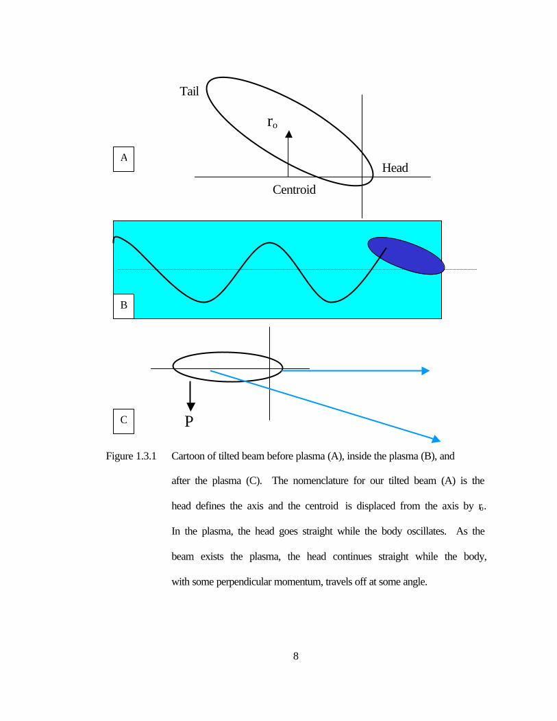
Figure 1.3.1 Cartoon of tilted beam before plasma (A), inside the plasma (B), and

after the plasma (C). The nomenclature for our tilted beam (A) is the

head defines the axis and the centroid is displaced from the axis by ro.

In the plasma, the head goes straight while the body oscillates. As the

beam exists the plasma, the head continues straight while the body,

with some perpendicular momentum, travels off at some angle.

ro

Head

Centroid

Tail

P⊥

A

B

C

9

Growth rates for the electron hose instability have been calculated based on a

simplified model [16]. For the E157 beam parameters, the growth rate of the

instability was predicted to be very rapid and therefore deleterious to the experiment.

The beam centroid offset was predicted to witness an amplification of 100-102x [17].

If these predictions were correct, the electron hose instability would not only increase

the difficulty of interpreting our experimental results, but it would also hinder the use

of PWFAs in future accelerators.

1.4 How might one look for the hose instability?

In the E157 experiment, the head of the beam blows out the plasma electrons

to form the ion column. If the beam enters the plasma with a tilt, then the centroid of

the beam will be offset in the ion column. If the electron hose instability exists, then

this offset will grow inside of the plasma. There exist two diagnostics that can resolve

the effects of the electron hose instability. They are the beam position monitors

(BPMs) and the streak camera. The BPMs will track the location of the beam

centroid, while the streak camera will temporally resolve the relative position of each

beam segment. Each diagnostic has its own advantages and disadvantages.

The BPMs track the position of the beam centroid as it drifts out of the plasma.

In order to look for hosing using this method, an energy scan data run must be taken.

An energy scan data run is when the plasma density is varied from 0 to 2x1014 cm-3

over 200 shots by varying the laser energy needed to ionize the Lithium vapor. By

10

plotting the centroid displacement as a function of distance after the plasma, the

trajectory of the centroid exiting the plasma can be calculated for each shot. Next you

plot the slope of the centroid’s trajectory vs. plasma density. If a hosing instability

exists, the slope of the trajectory will increase nonlinearly with plasma density.

The streak camera can be used to measure the head-tail offset for every shot.

If the laser is turned off (i.e. no plasma) then the initial tilt on the beam can be

measured. With the plasma turned on, the resultant beam tilt can be measured. This

will allow us to analyze how the plasma affects the entire beam, not just the centroid.

One difficulty with this measurement is keeping the beam aligned to the slit of the

streak camera. If the plasma imparts a large deflection to the beam, it can move the

image off of the slit.

One limitation of the current experimental setup is that the streak camera

diagnostic and four (out of five) BPMs are located after a large bending magnet. This

large bending magnet adds dispersion to the vertical plane that is used for the

experiment’s energy gain diagnostic. However, this magnet hampers the hosing

diagnostics because the analysis requires a pure drift space after the plasma. This

limits the analysis to the horizontal plane (x-axis) which does not gain dispersion

through the bending magnet. Results will show that a tail is in the x-y plane (section

4.1), but only the horizontal component of the tail will be quantified.

11

2 Theory of the Hosing Instability

2.1 Theory of the hose instability – Offset Oscillations.

The first step towards looking for the hosing instability is to calculate the

transverse motion of the beam in the absence of hosing. We will look at the special

case of a relativistic electron beam confined by an ion channel. The initial conditions

will be an electron beam and ion column with equal radii ro and uniform densities.

The electron beam density is denoted by nb and the ion column density is

np = ƒnb. (2.1.1)

The neutralization fraction, ƒ, is less than unity and it accounts for the under-dense

condition of the plasma density. We will assume that the ions are infinitely massive

(i.e. they are rigid) and that the ion column is centered on the z-axis. The beam

displacement, y(z,t), will have an initial displacement

yo = y(0,t). (2.1.2)

In the limit of small displacement, |yo| << ro, the electric field of the displaced charge

cylinders in the area region occupied by the cylinders is uniform with a magnitude

linearly proportional to the displacement. The electric field is given by

Ey(z,t) = -4p e nb y(z,t). (2.1.3)

This gives rise to a restoring force that is given by

Fy(z,t) = 4p e2 nb y(z,t). (2.1.4)

12

In addition to the force between the beam and the ion column, the beam position can

also change by convection. The net change in the transverse velocity of the beam is

ym

nez

ce

pyy

−

∂∂

−=∂∂

γπν

βτ

ν 24 (2.1.5)

Rearranging terms and defining the convective derivative and beam plasma frequency

z

cDtD

∂∂

+∂∂

= βτ

(2.1.6)

2/124

=

e

bb m

neγπ

ω (2.1.7)

we get

( )yDt

D y 2bƒω

ν−= (2.1.8)

We can similarly derive an expression for the change in y at a point

yzy

cty

νδδ

βδδ

+−= (2.1.9)

or

yDtDy

ν= (2.1.10)

Combining equations (2.1.8) and (2.1.10) in order to solve for the displacement as a

function of initial displacement gives

=2

2

DtyD

( )y2bƒω− (2.1.11)

13

or

( )yzy

czy

tc

ty 2

b2

222

2

2

ƒ2 ωδδ

βδδ

δδ

βδδ

−=++ (2.1.12)

Calculating a steady state solution by setting the time derivative to zero yields

ycz

y b

2

2

2

ƒ

−=

βω

δδ

(2.1.13)

The solution to this equation is

)cos( zkyy bo= (2.1.14)

where

)/(ƒ ck bb βω= (2.1.15)

This shows that if the electron beam enters the plasma with an offset, it will oscillate

harmonically about the center of the ion channel.

The plasma column in the E157 experiment, L, was 140cm long. The head of

the beam blows out the electrons and defines the plasma channel. If the beam has a

longitudinal-transverse correlation (i.e. tails or tilt), then the beam centroid is

displaced from the center of the plasma column. If the beam enters the plasma with an

offset of yo, then it will exit the plasma with an offset of

)cos(0 Lkyy bL = (2.1.16)

14

If Lkb does not equal an integer number of pi, then the centroid will gain some

perpendicular momentum as it exists the plasma. The slope of the centroid’s exit

trajectory is given by

)sin(0 Lkkyy bbL =& (2.1.17)

If an instability were present, we would expect to see a growth term in equation

(2.1.14).

)cos( zkeyy bA

o= (2.1.18)

The basic form of the solution is correct, but now we will go into a more rigorous

derivation for electron hosing.

2.2 Theory of Hosing II [16]

We will consider the relativistic beam propagation in an infinite, unmagnitized,

preionized, and uniform plasma of density np. The plasma is under-dense in relation

to the beam density, np < nb. We assume that the Budker condition, np >> nb/?2 is

satisfied. This implies that all beam electrons will undergo transverse oscillations at a

single “betatron frequency”, 2/1)2/( γωωβ p= . We will further assume a collisionless

plasma and that the plasma skin depth, c/? p, is much larger than the channel radius.

By using the “rigid beam” model and the “frozen field” approximation, we find that

the system response to a small perturbation, ?x(s,t), is described by a beam breakup

equation, where s is the longitudinal position of the beam in the laboratory frame and t

15

can be thought of as an index that labels a given slice of the beam (i.e. the head of the

beam is t = 0ps, and t = 4ps refers to the beam slice 4ps behind the head).

∫ ′′′−=

+

τ

β τδτξτττξγδδ

γδδ

0

2 ),()(),( sWskss x (2.2.1)

where the wakefield, W, is given by

)sin()( 2

3

τωω

τ oo

cW = (2.2.2)

kß is the betatron wave number and ?o=? p/(2)1/2. An asymptotic form for the solution

of equation (2.2.1) in the limit of strong focusing and a short bunch (i.e. picosecond

pulses) is obtained by the method of steepest descents [18]

+−≈

123cos263.0),( 2/1

πξτξ β

Aske

As Ao (2.2.3)

where

( )( )[ ] 3/122/3

43

),( τωτ β osksA = (2.2.4)

The solution in equation (2.2.3) is for the case when then entire beam is offset in the

plasma column. If the beam is tilted, the solution becomes [18]

+−≈

123cos341.0),(

2/3

πξτξ β

Aske

As Ao (2.2.5)

Figures 2.2.1 and 2.2.2 show how the centroid offset grows for different plasma

densities and how the instability grows for beam slices farther from the beam head

(i.e. increasing t). Notice how the growth factor, ocms ξτξ /),140( = , is significantly

16

reduced for the tilted case. Results from section 4.5 indicate that the beam centroid is

about 2ps back from the point of channel formation. The electrons that were to be

accelerated were about 4-6ps behind the beam centroid. Figure 2.2.3 shows how the

centroid and tail oscillates (t = 2, 4, and 6ps) inside of the plasma column and figure

2.2.4 shows how the centroid and tail oscillations will look downstream of the plasma

during a plasma density scan.

17

Figure 2.2.1 Parameter Space of Growth Factor for an Offset Beam in a

140cm long plasma

18

Figure 2.2.2 Parameter Space of Growth Factor for a Tilted Beam in

a 140cm long plasma

19

Figure 2.2.3 Oscillation of a tilted beam in a 2x1014 cm–3 plasma for a channel which

is formed 2ps before the centroid

20

Figure 2.2.4 Oscillation of a tilted beam at the end of a 140cm long plasma for

a channel that is formed 2ps before the centroid

21

2.3 Limitations to the Theory of Hosing

In the E157 experiment, the beam propagates in an underdense plasma and

both excites and witnesses the plasma wave. If two beams were used, one to drive the

wave and a second to witness the acceleration, the second beam would be propagating

in the ion-focused regime. The subtle difference is that a beam in under-dense plasma

creates an ion channel, as opposed to the ion-focused regime that assumes a pre-

formed ion channel. Although subtle, no hosing theory exists for the under-dense

regime; all have assumed the ion-focused regime. In the past, this approximation was

valid since the pulse length was greater than the plasma wavelength. In E157, the

pulse length is on the order of the plasma wavelength, therefore the dynamics of the

expelled electrons are important and the assumption of a preformed ion column is not

a valid one.

Valuable insight can still be gained from the equations, but they need to be

modified to take into account the formation of the ion column. A first approximation

is to modify the beam position parameter, t. t will no longer correspond to the

distance from the head of the beam, rather the distance from channel formation. Since

the channel can form near the beam centroid (figure 2.3.1) [19], the growth factor of

hosing is significantly reduced (e.g. reduce t from 8ps to 2ps in figure 2.2.2).

Therefore, one may not observe significant growth of the hosing instability in the

centroid motion of the beam. However, the tail of the beam could still suffer a

significant growth as seen in figures 2.2.3 and 2.2.4.

22

Figure 2.3.1 Dynamics of Ion Channel Formation. This is a 2-D Particle in Cell simulation of an electron beam (shown in blue) propagating in a plasma. The space charge of the beam expels plasma electrons radially to form an ion column. The radial electric field associated with the ion column is show in red. The magnitude of the field increases until all plasma electrons have been expelled and a pure ion column is left behind. At this point, known as “blow out”, the magnitude of the radial field is constant. As one can see, the point of channel formation (t = 0) is not the head of the beam, rather it is located part way into the beam.

Channel Forming

23

3 Experimental Setup

The principle components of the experimental apparatus are the Lithium

plasma source [20, 24], the optical transition radiators [21, 22, 24], the beam position

monitors [23], and an aerogel Cherenkov radiator [24]. A brief description of each

component will now be given. For a more detailed view of any specific component,

refer to the references given above.

Figure 3.0.1 Experimental Setup and Diagnostic Locations

0 1.07 2.63 11.8 12.63 25.96 40.29

Plasma exit

Dow

n OT

R

BPM

6130

Cherenkov

BPM

6160

BPM

6167

BPM

6170

24

3.1 Stanford Linear Accelerator (SLAC)

Before a description of the E157 experimental components is given, a brief

introduction to SLAC is necessitated. SLAC is operated under contract from the

United States Department of Energy (DOE) as a national basic research laboratory. Its

function is to probe the structure of matter at the atomic scale with x-rays and at much

smaller scales with electron and positron beams. The major facilities at SLAC are the

linac, End Station A, SPEAR and SSRL, PEP II, SLC, and the FFTB. The linac is a

three kilometer long accelerator capable of producing electron and positron beams

with energies up to 50 GeV. End Station A is for fixed target experiments. Early

work in End Station A showed that the constituents of the atomic nucleus, the proton

and neutron, are themselves composed of smaller, more fundamental objects called

quarks. The Stanford Synchrotron Radiation Laboratory (SSRL) uses the SPEAR

storage ring to produce intense x-ray and ultraviolet beams for probing matter on the

atomic scale. PEP II is a storage ring for a B meson factory in which an experiment,

BaBar, is seeking to answer why the universe is made of matter and not anti-matter.

The Stanford Linear Collider (SLC) in conjunction with the Stanford Large Detector

(SLD), analyzed collisions of 50 GeV electrons on 50 GeV positrons in order to

determine the mass and other properties of the Z0 particle, which is a carrier of the

weak force of subatomic physics. The Final Focus Test Beam (FFTB) is a facility for

research on future accelerator design. The E157 experiment is located inside the

FFTB.

25

3.2 Final Focus Test Beam (FFTB)

The FFTB was designed to be a facility to be used for the development and

study of optical systems, instrumentation, and techniques needed to produce the small

beam spot sizes required for future electron-positron colliders. The design consists of

five key sections. The first part is a matching section to match the beam that appears

at the end of the linac to the lattice of the FFTB beamline. This matching section also

has lens to match the betatron space of the beam to the second section, the chromatic

correction section. The second, third, and fourth sections are used to correct

chromatic and geometric aberrations on the beam. The final section is a telescope that

focus the beam down to a small spot size.

The optics of the FFTB consist of dipoles, quadrupoles, and sextapoles. In

order to focus the beam down to nanometer spot sizes, the optics needed to be aligned

to an accuracy on the order of a micron. The optics were mounted on 3-axis

positioners that allowed the optics to be moved ±1mm with 300nm resolution. To

complement these optics, diagnostics were needed to determine the spot size and

position of the beam along the beamline. These include torroids (to measure the

beam’s charge), wire scanners (to measure spot size), and BPMs (to measure the

beam’s posistion, Sec. 3.5). A diagram of the elements of the FFTB near interaction

point 1 is given in figure 3.2.1 while a full diagram of the FFTB elements is given in

appendix A.

26

IP1 – E157 Experiment

BPM 6130

X

Z

BPM 6160

BPM 6167

Cherenkov Radiator

UP OTR

Down OTR

Figure 3.2.1 Diagram of the FFTB near IP1 with relevant diagnostic locations marked

27

The E157 Experiment

3.3 Lithium plasma source

The two main components of the Li plasma source are the heat pipe oven and

the ionizing laser. The heat pipe oven consists of a stainless steel tube wrapped in

heater tapes. The inside is lined with a wire mesh and is partially filled with solid (at

room temperature) Lithium. Water jackets are placed at each end of the oven. A

helium buffer gas is used to constrain the Li vapor. The oven is heated to ~750ºC and

a Li vapor is formed. The vapor flows from the center of the oven (where it is the

hottest) to the water jackets (where it is the coolest). The mesh acts as a wick and

transports the Li back towards the center of the oven. The Helium gas, in conjunction

with the water jackets, constrains the Li vapor into a uniform column with sharp

boundaries. The end product of this heat pipe is a 1.4m long, uniform column of Li

vapor at a density of ~2x1015 cm-3.

An argon-fluoride excimer laser provides an ultraviolet pulse (193nm, 6.45eV)

to ionize the Li vapor via single photon absorption. The first ionization energy of Li is

5.392eV [25] with an ionization cross section of 1.8x10-18 cm-2. A 10-20ns laser pulse

is focused down the vapor column so that laser fluence is constant (photon absorption

is counteracted by reduced spot size). At the entrance of the plasma the laser cross-

section is approximately 16 mm2 whereas at the end it is approximately 8 mm2.

Because the laser fluence determines the plasma density, simply changing the output

pulse energy on the laser can vary the oven’s plasma density. This results in a 1.4m

28

long plasma column of with a variable density up to 6x1014 cm-3 as the laser energy is

varied from 0-40 mJ.

Figure 3.3.1 Diagram of Lithium Oven Setup and Depiction of Lithium Column

3.4 Optical Transition Radiators (OTR)

Two OTR diagnostics are employed in the E157 experiment, one 1 m before

the plasma and one 1m after the plasma. These diagnostics give us a single shot time-

integrated picture of the beam that allow us to measure the beam’s spot size in both

the x and y planes. The setup consists of a thin titanium foil placed at a 45º angle in

the beam line. An AF Micro-Nikkor 105mm f/2.8D lens is used to image the OTR

00 z

Li HeHe

Boundary Layers

OpticalWindow

CoolingJacket

CoolingJacket

Heater Wick

Insulation PumpHe

OpticalWindow

L

29

from the foil on to a 12-bit Photometrics Sensys CCD camera. The CCD has a pixel

size of 9µm x 9µm with an array size of 768 x 512. The spatial resolution of the setup

is approximately 20 µm. A computer is used to read out the images and it can acquire

date at 1 Hz.

OTR is one mechanism by which a charged particle can emit radiation. The

radiation is emitted when a charged particle passes from one medium into another.

For our case, the electron beam is propagating in a vacuum and then it enters a

titanium foil. When the beam is in vacuum it has certain field characteristics, and

when it is inside the titanium foil it has different field characteristics. As the beam

makes the transition into the foil, the fields must reorganize themselves. In the

process of reorganization, some of the field is “shed” off. Optical transition radiation

is this “shed” field [26].

OTR has been used extensively on low energy (MeV) beams, but people

thought that it would not be a viable diagnostic for high energy (GeV) beams. The

OTR has a peak at angles ?=1/?, which is small for 30 GeV beams (?=60000).

Because diffraction limited resolution goes as ?/?, the assumption was that high

energy beams could not be resolved. The misconception was that ? is the numerical

aperture of the lens, not the radiation source, and that there is significant radiation in

the wings of the OTR distribution profile. The E157 collaboration has proved this to

be correct by measuring spot sizes on the order of 30 µm. Figures 3.3.1 shows typical

upstream and downstream OTR images. The graininess of the downstream OTR

30

image is not from the beam, rather it results from the grain structure of the titanium

foil. Figure 3.3.2 shows how the image analysis routines in Matlab extract spot size

information from the images.

Figure 3.4.1 Upstream and Downstream OTR Images

180 µm

Bea

mlin

e Y

-axi

s

Beamline X-axis

Bea

mlin

e Y

-axi

s

Beamline X-axis

180 µm

Upstream OTR

Downstream OTR

31

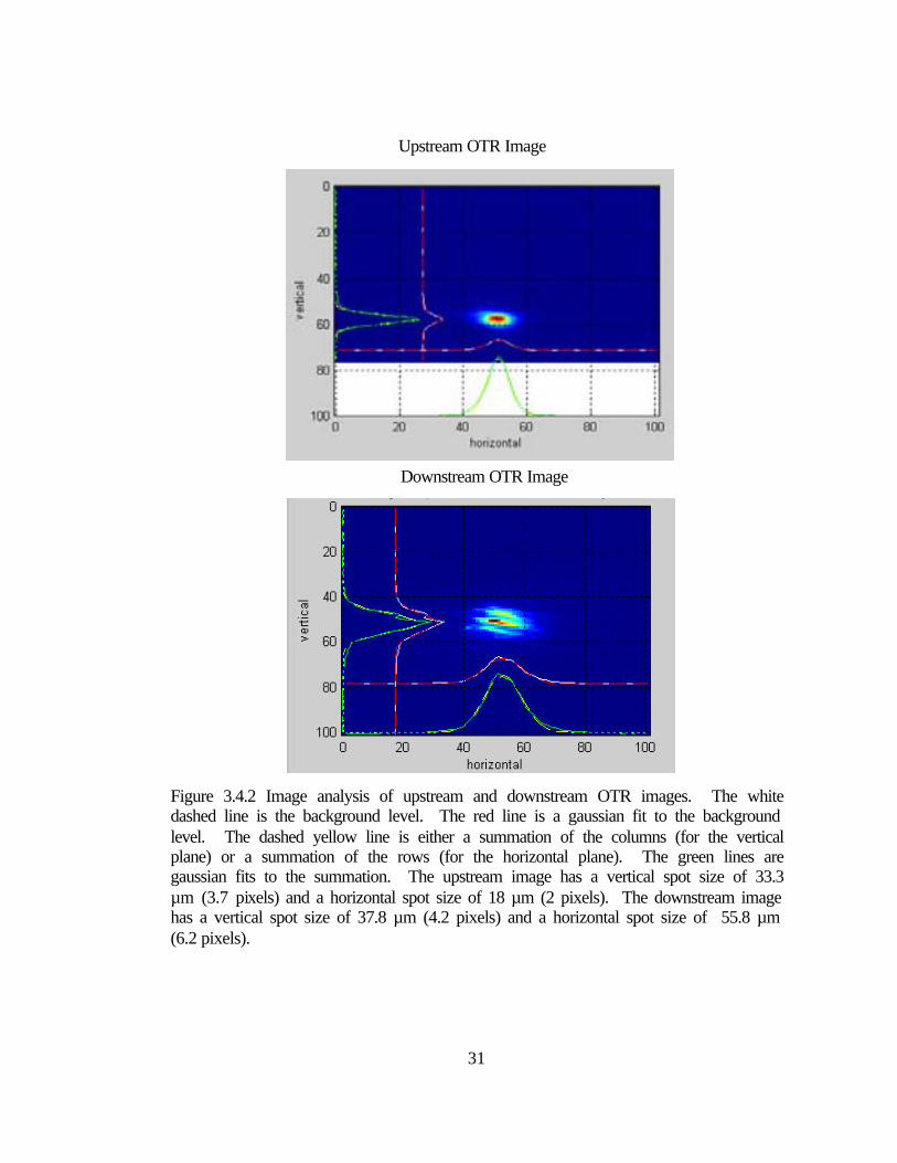
Figure 3.4.2 Image analysis of upstream and downstream OTR images. The white dashed line is the background level. The red line is a gaussian fit to the background level. The dashed yellow line is either a summation of the columns (for the vertical plane) or a summation of the rows (for the horizontal plane). The green lines are gaussian fits to the summation. The upstream image has a vertical spot size of 33.3 µm (3.7 pixels) and a horizontal spot size of 18 µm (2 pixels). The downstream image has a vertical spot size of 37.8 µm (4.2 pixels) and a horizontal spot size of 55.8 µm (6.2 pixels).

Upstream OTR Image

Downstream OTR Image

32

3.5 Beam Position Monitors (BPMs)

BPMs measure the beam’s position by coupling to the beams electromagnetic

field. They use four stripline antennas mounted in quadrature inside the beam pipe as

shown in figure 3.5.1.

The most common measurement is called the “difference over sum” method. In this

method, the radio frequency signal is peak rectified and stretched. The output is then

fed into circuitry that calculates positions from

xSDCBACBDA

X1)()(

++++−+

= (3.5.1)

ySDCBA

DCBAY

1)()(++++−+

= (3.5.2)

where

==o

o

yx

r

rSS0@;1

45@;2

)0,0()0,0( (3.5.3)

X

Y

Figure 3.5.1. Typical Stripline BPM

A

CD

B

e- beam beam pipe

33

In addition to calculating position, the BPMs can also be used to measure the beam

current.

BPMs are positioned all along the beam line in the FFTB. Several are

upstream of the plasma chamber and are used to align the beam with quadrupole

magnets and our plasma chamber. Five BPMs located downstream of the plasma

chamber are used to measure the trajectory of the beam as it exists the plasma.

3.6 Aerogel Cherenkov Radiator

Cherenkov radiation is emitted whenever charged particles pass through a

medium with a velocity that exceeds the velocity of light in that medium.

v > vt = c/n (3.6.1)

where v is the particle’s velocity (in our case v=c), vt is the threshold velocity, and n is

the index of refraction of the medium. One can see that Cherenkov radiation will be

emitted anytime a relativistic beam passes through any medium (n>1). The light is

emitted at a constant angle with respect to the particle’s trajectory.

)(11

)cos( cvfornnvn

cvvt =====

βδ (3.6.2)

This emission is similar to the bow shock created during supersonic flight.

In our experiment, we use the Cherenkov light as part of our energy gain

diagnostic. The electron beam exists the plasma and drifts through an energy

dispersive magnet. The beam then passes through the aerogel and emits Cherenkov

34

radiation. The light is transported approximately 15m to an optical table outside of the

FFTB. The light passes through a beam splitter and a small fraction of the light is sent

to a CCD camera for time-integrated images of the beam figure 3.6.1 (similar to the

OTR images). The remaining light passes through a beam splitter again and one arm

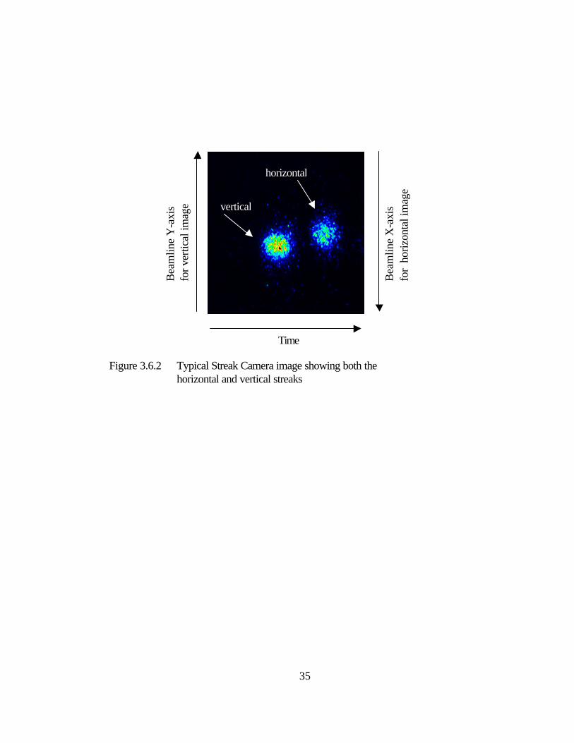
is rotated 90 degrees. The two paths are recombined and sent to the streak camera.

The 90 degree rotation allows us to streak both the energy dispersive plane (y-axis)

and the non-dispersive plane (x-axis) simultaneously figure 3.6.2. Figure 3.6.3 shows

the layout of the optical table. The streak camera has a temporal resolution of one

picosecond and a spatial resolution of ~100 µm. My analysis will use the non-

dispersive plane on the streak camera in order to resolve head-tail offsets.

Figure 3.6.1 Time Integrated Cherenkov Image depicting the parts of the beam seen by the horizontal and vertical slits on the streak camera

Slit Locations

700 µm

Beamline X-axis

Bea

mlin

e Y

-axi

s

35

Time

Figure 3.6.2 Typical Streak Camera image showing both the horizontal and vertical streaks

vertical

horizontal B

eam

line

Y-a

xis

for v

ertic

al im

age

Bea

mlin

e X

-axi

s fo

r ho

rizon

tal i

mag

e

36

Figure 3.6.3 Diagram of Cherenkov radiation detector setup. The light radiated from the aerogel enters the setup at �. It is reflected off of a mirror towards beam splitter �. Part of the light is sent to the image rotator � via path � while the other part is directed towards beam splitter �. Part of light off of beam splitter � is sent to a CCD camera � for time integrated Cherenkov images while the rest is directed towards beam splitter � via path �. The image on path � passes through an image rotator � where it is rotated 90 degrees (the unrotated path is shown in light blue while the rotated image path is shown in purple). Both the unrotated and rotated images are combined at beam splitter �. The combined images (slightly delayed in time from each other) are then sent to the streak camera � for time-resolved analysis.

�

�

�

�

�

� �

�

�

�

�

37

4 Results

4.1 Initial Beam Condition

One of the major highlights of the E157 experiment was the advance made in

beam diagnostics. These diagnostics allowed the accelerator physicists to see details

of the beam dynamics they had not seen before. The lowest order concern for the

experiment was delivering a beam to our plasma with a specified energy and spot size.

These requirements were readily attainable since the energy was determined by the

linac settings and the spot size was determined by adjusting the beam optics to focus

the beam at the plasma entrance. With the knowledge that the electron hosing

instability might be a problem for our experiment, we were also concerned about a

longitudinal transverse correlation on the beam.

With the available E157 diagnostics, a beam tilt could be quantified by time

resolving laser off (i.e. no plasma) data. Because the streak camera is located after the

energy (or vertical plane) dispersive bend magnet, we will look at streak data from the

horizontal plane (no dispersion). The first step is to slice up the streaked image in 1ps

bins. Next, analyze each slice to find its mean position. Finally, a tilt implies that the

mean position of each slice will change in time. Figure 4.1.1 shows a streak camera

image, where the horizontal streak image has been selected. The lines on the image

illustrate how the data analysis software slices up the time-resolved image.

38

The results of the analysis for two single events are plotted with the x-axis being time

and the y-axis being mean position. –4ps is the head of the beam, and +5ps is the tail

end of the beam. To help visualize the beam tilt, imagine that you are flying down the

Horizontal Laser Off Streak Data

Time

x

Ø Cut beam up into slices Ø Analyze each slice to find <x> Ø A tilt implies <x> will move in time

Figure 4.1.1 Streak Camera Data

39

beam line looking down at the electron bunch. You will see the back of the bunch is

not in line with the head of the bunch, rather it is displaced to the side.

The total results for a single run of 25 consecutive shots are given in figure 4.1.3.

Every data point is plotted for each picosecond bin. The solid line drawn through the

points represent the mean of all 25 shots for each time step. The two dashed lines

represent the mean ± rms for each time step.

Analysis of Single Shots

Figure 4.1.2 Tilted Beams (N=2x1010 e-; s xDN=110µm)

Head Head

Tail Tail

Figure 4.1.3 Average of 25 laser off shots (N=2x1010 e-; s xDN=110µm)

40

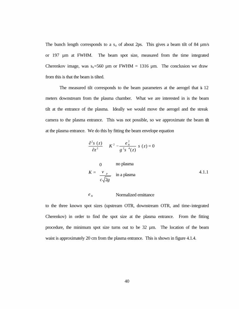
The bunch length corresponds to a sz of about 2ps. This gives a beam tilt of 84 µm/s

or 197 µm at FWHM. The beam spot size, measured from the time integrated

Cherenkov image, was sx=560 µm or FWHM = 1316 µm. The conclusion we draw

from this is that the beam is tilted.

The measured tilt corresponds to the beam parameters at the aerogel that is 12

meters downstream from the plasma chamber. What we are interested in is the beam

tilt at the entrance of the plasma. Ideally we would move the aerogel and the streak

camera to the plasma entrance. This was not possible, so we approximate the beam tilt

at the plasma entrance. We do this by fitting the beam envelope equation

N

p

N

c

K

zz

Kz

z

ε

γ

ϖ

σσγεσ

=

=

−+

∂∂

2

0

0)()(

)(42

22

2

2

4.1.1

to the three known spot sizes (upstream OTR, downstream OTR, and time-integrated

Cherenkov) in order to find the spot size at the plasma entrance. From the fitting

procedure, the minimum spot size turns out to be 32 µm. The location of the beam

waist is approximately 20 cm from the plasma entrance. This is shown in figure 4.1.4.

no plasma in a plasma

Normalized emittance

41

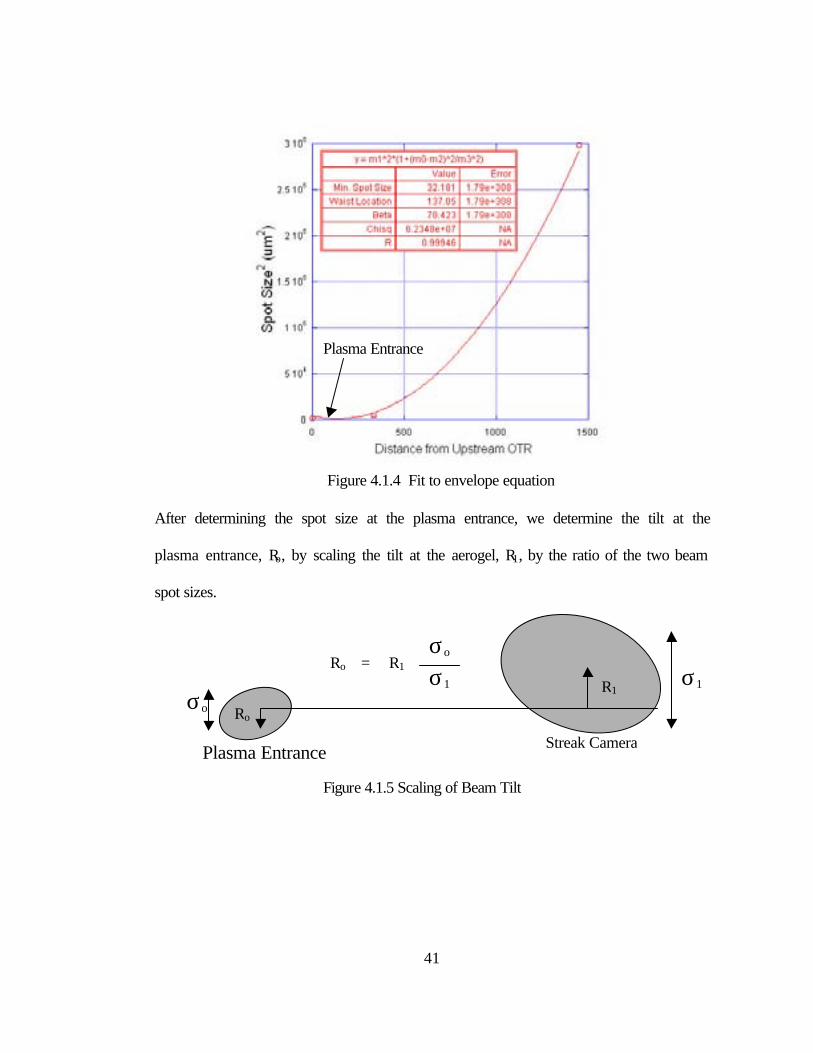
After determining the spot size at the plasma entrance, we determine the tilt at the

plasma entrance, Ro, by scaling the tilt at the aerogel, R1, by the ratio of the two beam

spot sizes.

Figure 4.1.4 Fit to envelope equation

Plasma Entrance

Ro

R1σ1

σo

σo

σ1

R1Ro =

Streak Camera Plasma Entrance

Figure 4.1.5 Scaling of Beam Tilt

42

The values for the offset at the plasma entrance for the 25 shots are

4.2 Centroid Oscillations

Although our analysis is limited to the horizontal plane (due to the dispersive

bending magnet), a beam tail generally lies in both the vertical and horizontal planes.

Figure 4.2.1 shows two upstream OTR images of beams with large tails. With the

knowledge that the beam coming into the plasma is tilted, we would expect the

trajectory of the exiting beam centroid to oscillate (equation 2.1.17). The data in

figures 4.2.2 and 4.2.3 was energy scan data. The plasma density (x-axis) was varied

by varying the ionizing laser energy. Figure 4.2.2 shows centroid oscillations in both

the horizontal and vertical planes just after the plasma on BPM 6130. Figure 4.2.3

0

1

2

3

4

5

6

7

8

9

10

5 10 15 20 25 30

Cen

troid

Off

set a

t 1 s

igm

a (u

m)

Shot Number

Figure 4.1.6 Centroid offset at plasma entrance (N=2x1010 e-; s xUP=36µm)

43

shows the horizontal deviation of the beam centroid from the laser off position on the

downstream OTR (DNOTR). In general, neither the spot size nor the centroid

oscillations in both the horizontal (x) nor the vertical (y) planes were in exact phase

with respect to each other because of the large difference in the beam emittance in

these two planes.

Tail

Centroid

Tail

Centroid

Bea

mlin

e Y

-axi

s

Bea

mlin

e Y

-axi

s

Beamline x-axis Beamline x-axis

Figure 4.2.2 Centroid Oscillations on BPM 6130 for both the horizontal and vertical planes. The x-axis is the laser energy (plasma density) and the y-axis is the position of the beam centroid measured by the BPM.

Figure 4.2.1 Upstream OTR images showing a tail that lies in both the horizontal and vertical plane (with respect to the beam centroid).

44

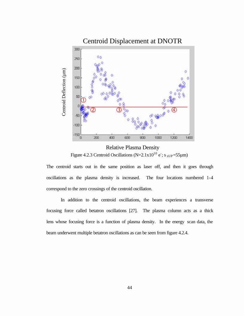
The centroid starts out in the same position as laser off, and then it goes through

oscillations as the plasma density is increased. The four locations numbered 1-4

correspond to the zero crossings of the centroid oscillation.

In addition to the centroid oscillations, the beam experiences a transverse

focusing force called betatron oscillations [27]. The plasma column acts as a thick

lens whose focusing force is a function of plasma density. In the energy scan data, the

beam underwent multiple betatron oscillations as can be seen from figure 4.2.4.

Centroid Displacement at DNOTR

��

� �

Relative Plasma Density Figure 4.2.3 Centroid Oscillations (N=2.1x1010 e-; s xUP=55µm)

Cen

troid

Def

lect

ion

(µm

)

45

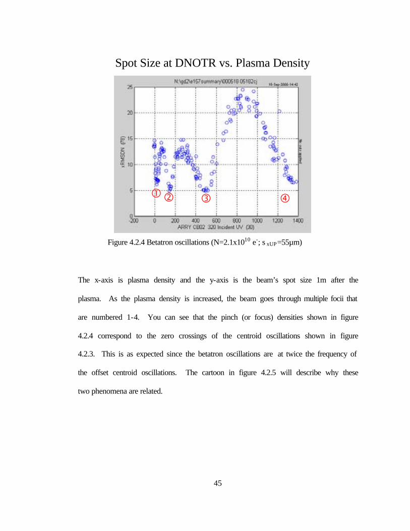
The x-axis is plasma density and the y-axis is the beam’s spot size 1m after the

plasma. As the plasma density is increased, the beam goes through multiple focii that

are numbered 1-4. You can see that the pinch (or focus) densities shown in figure

4.2.4 correspond to the zero crossings of the centroid oscillations shown in figure

4.2.3. This is as expected since the betatron oscillations are at twice the frequency of

the offset centroid oscillations. The cartoon in figure 4.2.5 will describe why these

two phenomena are related.

Spot Size at DNOTR vs. Plasma Density

� � � �

Figure 4.2.4 Betatron oscillations (N=2.1x1010 e-; s xUP=55µm)

46

As one can see, all electrons are oscillating across the axis. The difference is that

when there are electrons on both sides of the axis, the beam appears to be focusing and

defocusing whereas the tail electrons only appear to oscillate across the axis.

1) Initial Beam Condition at the plasma exit. Note red electrons start off above the axis and blue ones below 2) At the first pinch – all electrons moved towards the axis. Notice the zero crossing of the centroid oscillation. The electrons have a maximum transverse or perpendicular momentum. This beam will defocus at the Cherenkov detector 3) Moving away from the pinch. The beam has blown back up to its original size (one oscillation) and the centroid (tail) has made half an oscillation. This is the “so called” p phase advance condition. The tail is now below the axis and the electrons have a minimum transverse or perpendicular momentum. 4) The beam goes through a second pinch and the centroid goes through a second zero crossing. Again the electrons have a large perpendicular momentum at the plasma exit.

Head Tail

Figure 4.2.5 Single electron motion within the beam at the plasma exit

47

4.3 Tail Flipping

Following the above discussion, the dynamics of the beam can be studied by

temporally resolving the beam near a pinch at the Cherenkov detector. This

corresponds to a multiple of p phase advance for the beam envelope as it goes through

the plasma since a well focused beam at the Cherenkov is only obtained when the

beam exits the plasma more-or-less as it entered. As the beam passes through a pinch,

the tail should flip from one side of the head to the other. Data was analyzed from

both the 4th pinch and the 3rd pinch. The data was divided into bins according to

proximity to the pinch. In each bin, the shots were analyzed to determine the

horizontal mean position vs. position in the beam (head, tail, centroid, etc.) The data

shows the tail moving from one side of the head to the other at the 3rd pinch. At the 4th

pinch, the tail goes back to its original side.

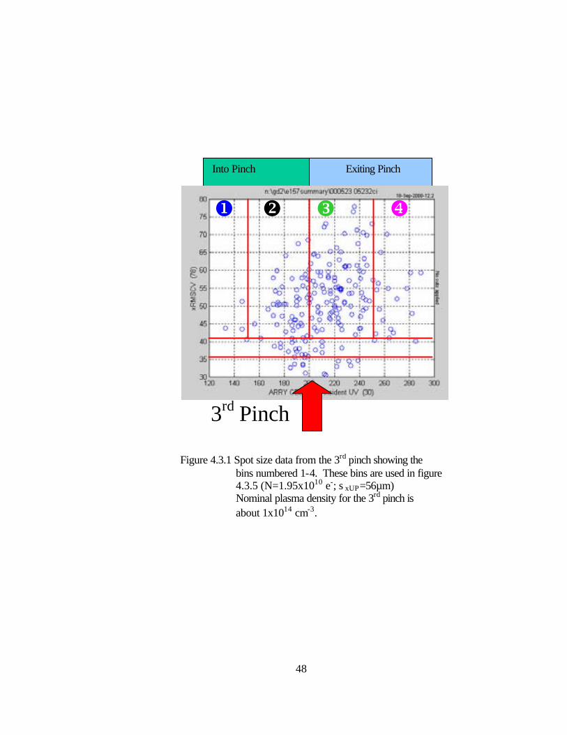
Figures 4.3.1 and 4.3.2 show how the data was binned for analysis. The

bottom red line corresponding to xRMS of 36 denotes the laser off spot size. Shots

with spot sizes below this line are considered to be at the transparency condition. The

upper horizontal red line is an arbitrarily chosen criteria to say that any shots with a

spot size above this line are defocusing. The vertical lines separate defocused shot

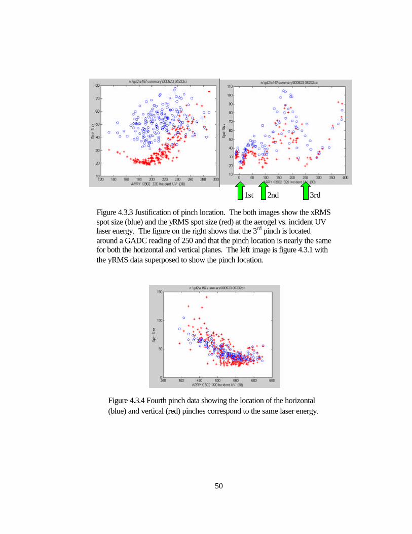
into group that are either coming into or exiting the pinch. Figure 4.3.3 gives

justification for the 3rd and 4th pinch locations. Figures 4.3.5 and 4.3.6 show the tail

flipping at the different pinches.

48

3rd Pinch

Into Pinch Exiting Pinch

Figure 4.3.1 Spot size data from the 3rd pinch showing the bins numbered 1-4. These bins are used in figure 4.3.5 (N=1.95x1010 e-; s xUP=56µm) Nominal plasma density for the 3rd pinch is about 1x1014 cm-3.

u v x w

49

4th Pinch

Into Pinch Exiting Pinch

Figure 4.3.2 Spot size data from the 4th pinch showing the bins numbered 5-9. These bins are used in figure 4.3.6. (N=1.95x1010 e-; s xUP=54µm)

Nominal plasma density for the 4th pinch is about 2x1014 cm-3.

| } z { y

50

1st 2nd 3rd

Figure 4.3.3 Justification of pinch location. The both images show the xRMS spot size (blue) and the yRMS spot size (red) at the aerogel vs. incident UV laser energy. The figure on the right shows that the 3rd pinch is located around a GADC reading of 250 and that the pinch location is nearly the same for both the horizontal and vertical planes. The left image is figure 4.3.1 with the yRMS data superposed to show the pinch location.

Figure 4.3.4 Fourth pinch data showing the location of the horizontal (blue) and vertical (red) pinches correspond to the same laser energy.

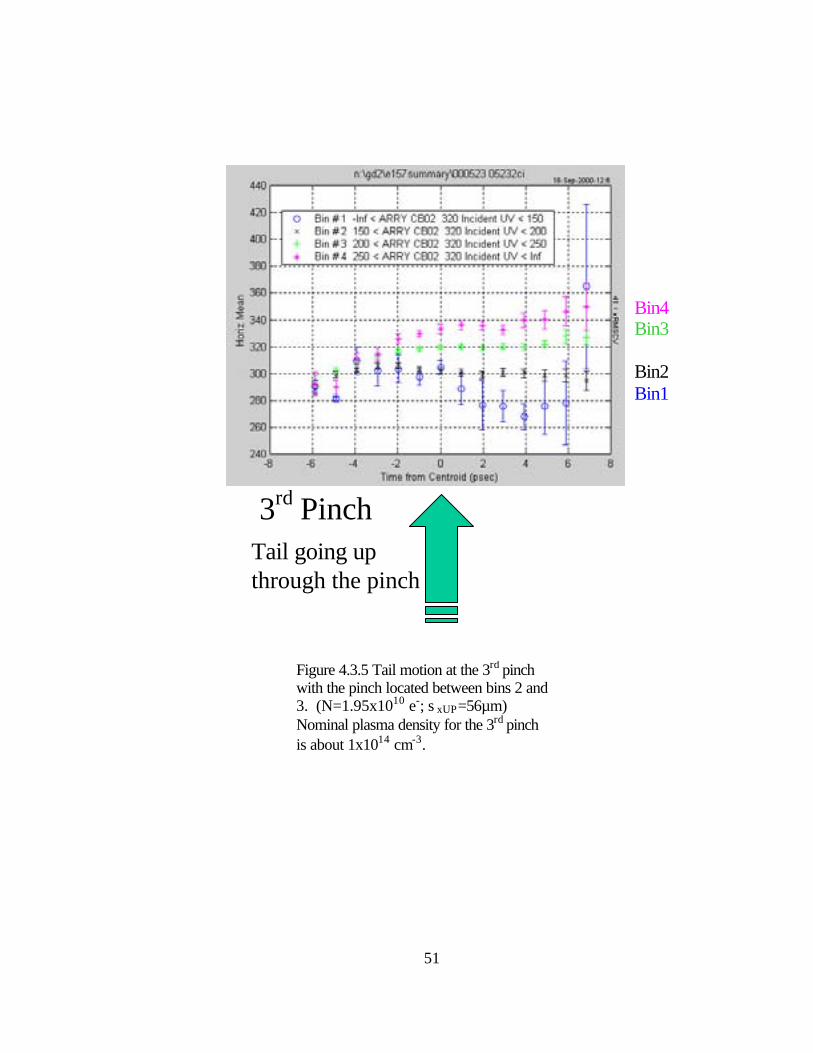
51

3rd Pinch

Bin4 Bin3 Bin2 Bin1

Tail going up through the pinch

Figure 4.3.5 Tail motion at the 3rd pinch with the pinch located between bins 2 and 3. (N=1.95x1010 e-; s xUP=56µm) Nominal plasma density for the 3rd pinch is about 1x1014 cm-3.

52

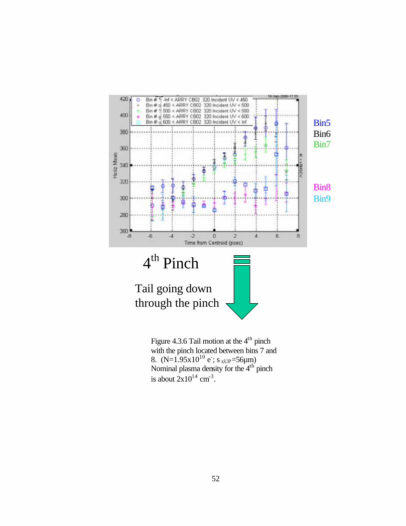
4th Pinch

Bin5 Bin6 Bin7 Bin8 Bin9

Tail going down through the pinch

Figure 4.3.6 Tail motion at the 4th pinch with the pinch located between bins 7 and 8. (N=1.95x1010 e-; s xUP=56µm) Nominal plasma density for the 4th pinch is about 2x1014 cm-3.

53

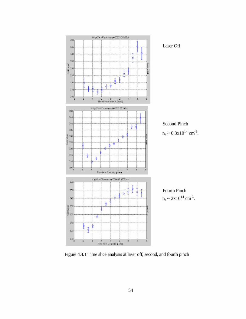
4.4 Tail Growth on Streak Camera Diagnostic

After showing that the beam is tilted and that this tilt results in tail flipping, we

now want to determine if we are experiencing a hosing instability. We will do this by

looking at the streak camera data for three cases. The first case will be laser off data.

This will determine the initial tilt on the beam. The other two cases are at two

different plasma densities; the second and fourth pinches at the Cherenkov detector.

The second and fourth pinches were chosen because they are both an integer number

of betatron oscillations and an integer number of tail oscillations. Only data that

satisfied a transparency condition, where the beam spot size was equal to or slightly

smaller than the laser off spot size, was chosen. The laser off spot size was ~36

pixels and the data cut at the 4th pinch can be seen as the lower red bar in figure 4.3.2.

The hypothesis is if an instability exists, then the magnitude of the head tail offset

should rapidly grow with increasing plasma density (i.e. laser off ? 2nd pinch ? 4th

pinch). Figures 4.4.1 shows the time slice analysis of the beam at the laser off, 2nd,

and 4th pinches respectively. The results show that there are not signs of significant

growth up to the fourth pinch, the operating point of the experiment.

54

Laser Off

Second Pinch

Fourth Pinch

Figure 4.4.1 Time slice analysis at laser off, second, and fourth pinch

ne ~ 0.3x1014 cm-3.

ne ~ 2x1014 cm-3.

55

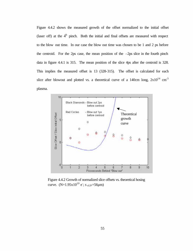
Figure 4.4.2 shows the measured growth of the offset normalized to the initial offset

(laser off) at the 4th pinch. Both the initial and final offsets are measured with respect

to the blow out time. In our case the blow out time was chosen to be 1 and 2 ps before

the centroid. For the 2ps case, the mean position of the –2ps slice in the fourth pinch

data in figure 4.4.1 is 315. The mean position of the slice 4ps after the centroid is 328.

This implies the measured offset is 13 (328-315). The offset is calculated for each

slice after blowout and plotted vs. a theoretical curve of a 140cm long, 2x1014 cm-3

plasma.

Theoretical growth curve

Figure 4.4.2 Growth of normalized slice offsets vs. theoretical hosing curve. (N=1.95x1010 e-; s xUP=56µm)

56

4.5 BPM Data for a High Density Run

One data run in the E157 experiment achieved a density higher than any other

run. Whereas most runs could only achieve a density of 2x1014 cm-3, one run achieved

a density of approximately 6x1014 cm-3. This is important because the hosing growth

rate increases rapidly with increasing density. Because this run was energy scan data,

the centroid motion experienced large displacements. These kicks were large enough

to steer the beam off of the streak camera slit, rendering the streak camera data

unusable. This mandated the use of BPMs to look for the hosing instability.

To analyze this data, we follow the oscillations of the beam exiting the plasma

as measured by the downstream OTR and the beam position monitors 6130, 6160,

6167, and 6170 (figure 4.5.1). For each shot, the deviation from laser off position is

calculated and this deviation is plotted versus the BPM’s (or downstream OTR)

position relative to the exit of the plasma. Figure 4.5.2 shows typical beam trajectory

leaving the plasma. A straight line fit is made to the five points (a straight line

indicates that upon leaving the plasma, the beam centroid travels ballistically), and the

slope of the exit trajectory is found. Figure 4.5.3 shows a plot of the slope of the

beam’s exit trajectory versus incident laser energy for all 200 shots.

57

A B

C D

E

Diagnostic name with distance from plasma exit. A – Downstream OTR 1.07m B – BPM 6130x 2.63m C – BPM 6160x 12.63m D – BPM 6167x 25.96m E – BPM 6170x 40.29m

Figure 4.5.1 Oscillations of beam centroid after plasma exit as measured on downstream OTR and on BPMs 6130, 6160, 6167, and 6170. The x-axis is the incident UV laser energy and the y-axis is the transverse position of the beam centroid. (N=2x1010 e-; s xUP=36µm)

58

Figure 4.5.2 Beam trajectory exiting plasma (N=2x1010 e-; s xUP=36µm)

BPM 6170

BPM 6167

BPM 6160

BPM 6130

Downstream OTR

Figure 4.5.3 Slope of the beams exit trajectory as a function of laser energy (plasma density) (N=2x1010 e-; s xUP=36µm)

59

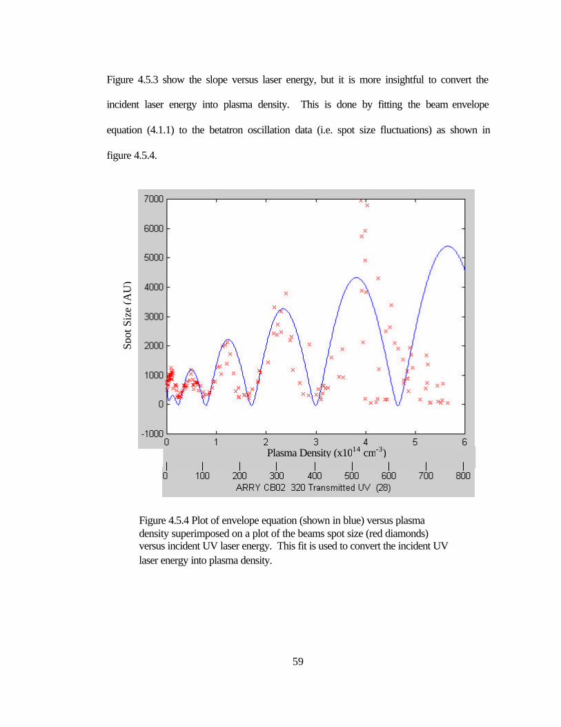
Figure 4.5.3 show the slope versus laser energy, but it is more insightful to convert the

incident laser energy into plasma density. This is done by fitting the beam envelope

equation (4.1.1) to the betatron oscillation data (i.e. spot size fluctuations) as shown in

figure 4.5.4.

Plasma Density (x1014 cm-3)

Figure 4.5.4 Plot of envelope equation (shown in blue) versus plasma density superimposed on a plot of the beams spot size (red diamonds) versus incident UV laser energy. This fit is used to convert the incident UV laser energy into plasma density.

Spot

Siz

e (A

U)

60

The equation for the exit trajectories slope in the absence of hosing (2.1.17) has four

variables: the slope, r’; the initial offset, ro; the plasma density, kß; and the plasma

column length, s. The only unknown is the initial offset. By applying the formula for

centroid oscillations with no growth (2.1.17) and solving for ro at low densities, we

find that the initial offset is about 24 µm.

The slope is the ratio of the beams transverse energy to its longitudinal energy.

||||2

2

γγ

γγ ⊥⊥ ==′

cmcm

re

e 4.5.1

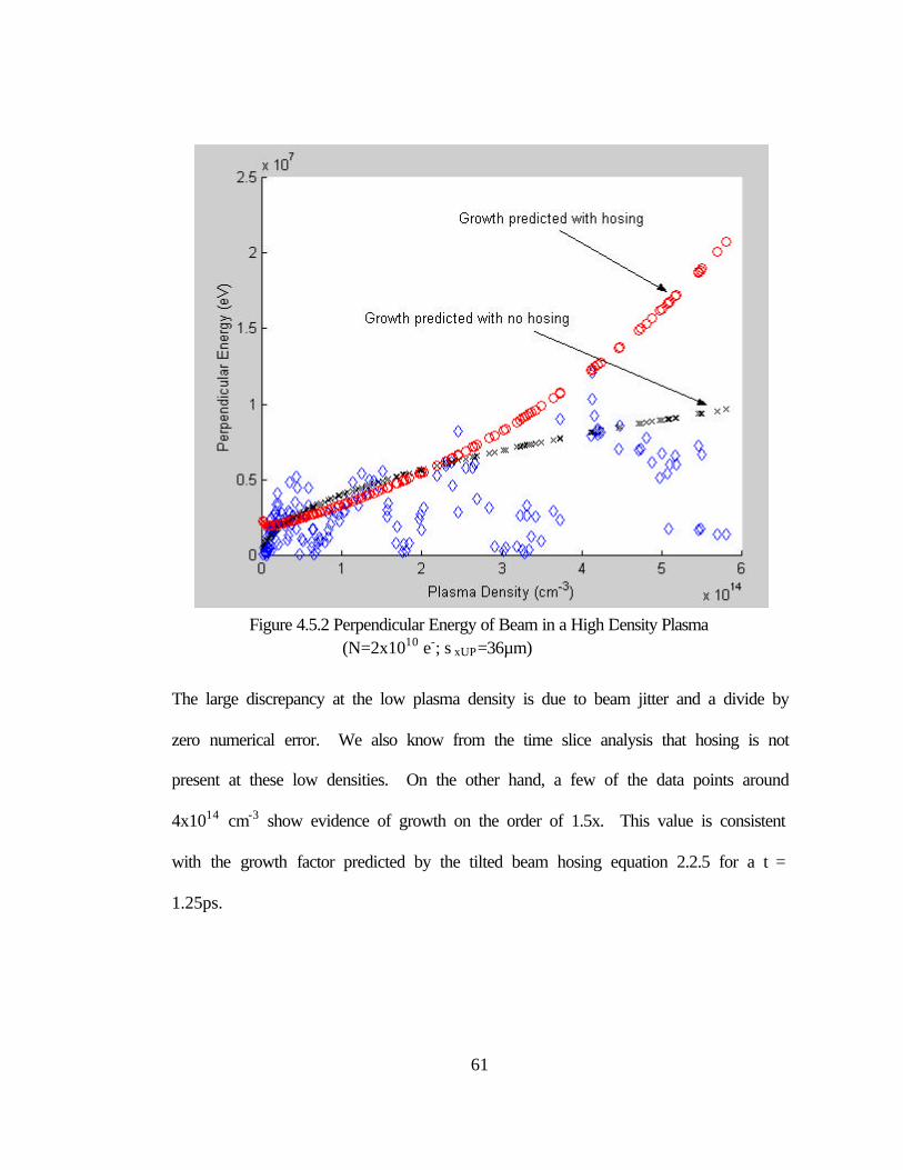
Figure 4.5.2 shows the calculated perpendicular energy of the beam (found from the

slope trajectory) plotted vs. plasma density. The blue diamonds represent calculated

values and the black x’s represents a theoretical envelope (neglecting the sinusoidal

term for clarity) curve of perpendicular energy in absence of hosing .

2mckrE o β=⊥ 4.5.2

The red circles represent a theoretical envelope (neglecting the sinusoidal term for

clarity) curve for perpendicular energy with hosing.

22/3

341.0 mckrAe

E o

A

β=⊥

The slice index t was chosen to be 1.25ps so that the theoretical curve matched a data

point at the plasma density of 4*1014 cm-3. A small value of t is expected since “blow

out” occurs near the centroid and BPMs measure the position of the centroid.

61

The large discrepancy at the low plasma density is due to beam jitter and a divide by

zero numerical error. We also know from the time slice analysis that hosing is not

present at these low densities. On the other hand, a few of the data points around

4x1014 cm-3 show evidence of growth on the order of 1.5x. This value is consistent

with the growth factor predicted by the tilted beam hosing equation 2.2.5 for a t =

1.25ps.

Figure 4.5.2 Perpendicular Energy of Beam in a High Density Plasma (N=2x1010 e-; s xUP=36µm)

62

5 Conclusion 5.1 Summary

A subset of the transverse dynamics of an ultra-relativistic electron beam

propagating through a meter long plasma has been experimentally measured. The

electron hosing instability arises when electrons are offset in an ion column. In a

single bunch PWFA experiment, a beam tilt will result in offset electrons. Time-slice

analysis of the electron bunch has quantified a head-tail offset (i.e. tilt). Further

analysis has shown the tail off the beam oscillating inside the plasma. Finally, the

magnitude of the oscillation was not observed to significantly grow up to the operating

plasma density of the E157 experiment. In other words, there is no evidence of the

electron hosing instability at the operating parameters of the E157 experiment. Recent

simulations by E. Dodd corroborate the above statement [28]. There is possible

evidence of the hosing instability in a single high-density plasma run, but further data

is needed at such a high density to be conclusive.

5.2 Future Directions

An upcoming experiment at SLAC will provide the opportunity to expand on

these results [29]. First, an imaging spectrometer will be constructed that will image

the beam from the output of the plasma onto the aerogel. This will allow us to analyze

the beam at the exit of the plasma as opposed to analyzing it after 12 meters of drift.

63

A second benefit will be the analysis of positron beams. In an analogous situation to

ion channel formation with electron beams, positron beams will create a channel

where electrons rush in. The transverse dynamics of a positron beam will be rich with

physics that will be both challenging and rewarding to analyze.

64

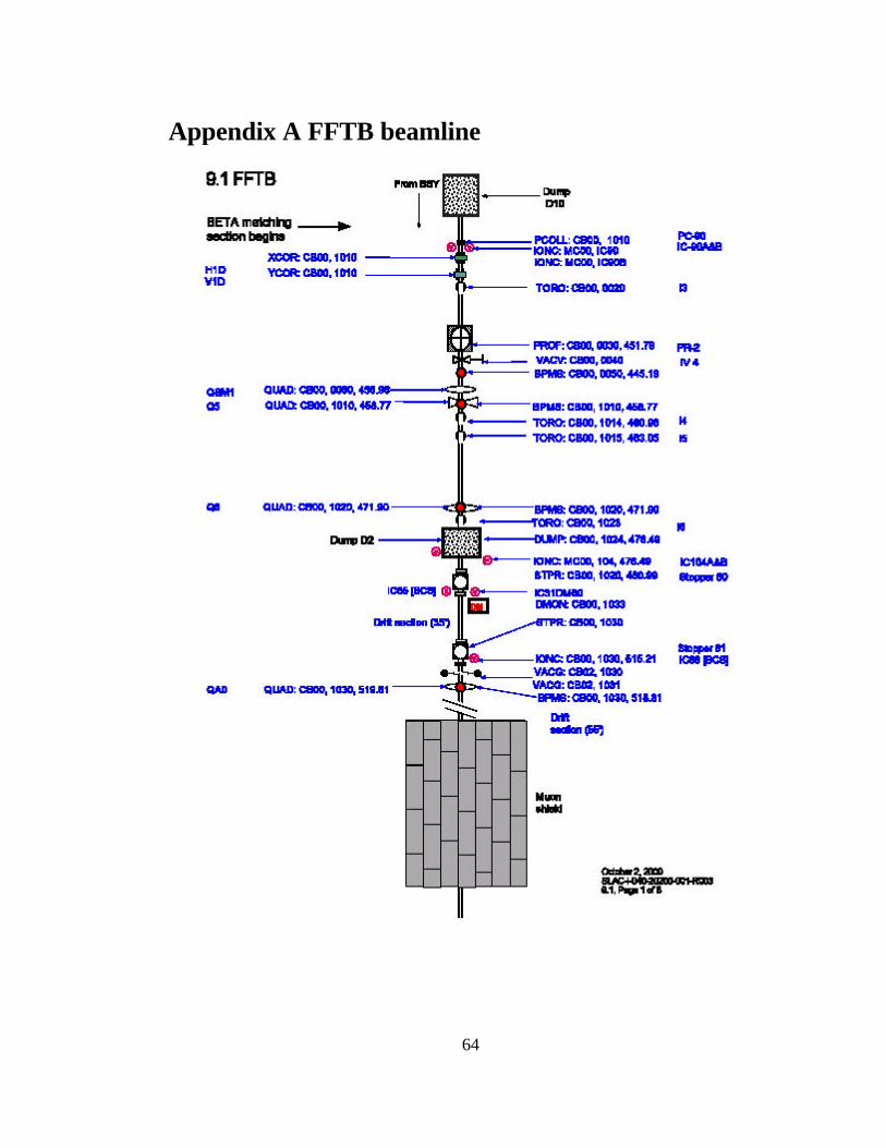
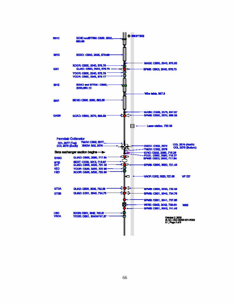
Appendix A FFTB beamline

65

66

67

68

69

70

71

72

Appendix B Typical Electron Beam Parameters Number of electrons per bunch 1.8-2.0x1010 Bunch Energy 28.5 GeV Gamma 55773 Bunch Radius 50 µm Bunch Length 0.7 mm 2.3 ps Normalized Emittance x 5x10-5 m rad Normalized Emittance y 0.5x10-5 m rad

73

Bibliography [1] J.M. Dawson, “Nonlinear electron oscillations in a cold plasma,” Phys. Rev.,

vol. 133, pp. 383-387, 1959. [2] E. Esarey, P. Sprangle, J. Krall et al, “Overview of plasma based accelerator

concepts,” IEEE Transactions on Plasma Science, 24, 252 (1996). [3] C.E. Clayton, K.A. Marsh, A. Dyson, M. Everett, A. Lal, W.P. Leemans, R.

Williams, and C. Joshi, “Ultrahigh-gradient acceleration on injected electrons by laser-excited relativistic electron plasma waves,” Phys. Rev. Lett. vol. 70, pp. 37-40, 1993.

[4] W. B. Mori, “Computer simulations on the acceleration of electrons by fast

large-amplitude plasma waves driven by laser beams,” Master’s Thesis, Univ. California Los Angeles, 1984.

[5] K. Nakajima, D. Fisher, T. Kawakubo, H. Nakanishi, A. Ogata, Y. Kato, Y.

Kitagawa, R. Kodama, K. Mima, H. Shiraga, K. Suzuki, K. Yamakawa, T. Zhang, Y. Sakawa, T. Shoji, Y. Nishida, N. Yugami, M. Downer, and T. Tajima, “Observation of ultrahigh gradient electron acceleration by a self-modulated intense short laser pulse,” Phys. Rev. Lett. vol. 74, pp. 4428-4431, 1995.

[6] Katsouleas, T.; Lee, S.; Chattopadhyay, S.; Leemans, W.; Assmann, R.; Chen,

P.; Decker, F.J.; Iverson, R.; Kotseroglou, T.; Raimondi, P.; Raubenheimer, T.; Eokni, S.; Siemann, R.H.; Walz, D.; Whittum, D.; Clayton, C.; Joshi, C.; Marsh, K.; Mori, W.; Wang, G., “ A proposal for a 1 GeV plasma-wakefield acceleration experiment at SLAC,” Proceedings of the 1997 Particle Accelerator Conference, Vancouver, BC, Canada, 12-16 May 1997. Piscataway, NJ, USA: IEEE, 1998. p.687-9 vol.1

[7] T.O. Raubenheimer et al, “Zeroth order design report for the next linear

collider,” SLAC-Report-474 May 1996 [8] J.J. Su, T. Katsouleas, J.M. Dawson, and R. Fedele, “Plasma lenses for

focusing particle beams,” Phys. Rev. A., vol. 41. pp. 3321, 1990. [9] P. Chen, K. Oide, A.M. Sessler, and S.S. Yu, “Plasma based adiabatic

focuser,” Phys. Rev. Lett., vol. 64, pp. 1231, 1990.

74

[10] W.A. Barletta, “Linear emittance damper with megagauss fields,” Proceedings of the Workshop on New Developments in Particle Acceleration Techniques, (CERN Service d’Information, Orsay), pp. 544, 1987.

[11] K. Takayama, S. Hiramatsu, “Ion-channel guiding in a steady-state free-

electron laser,” Phys. Rev. A, vol. 37, pp. 173, 1988. [12] S. Hiramatsu et al, “Proposal for an X-band single-stage FEL,” Nucl. Instrum.

Methods Phys. Res., Sec. A., vol. 285, pp. 83, 1989 [13] K.J. O’Brien, “Theory of the ion-hose instability,” Journal of Applied Physics,

vol.65, (no.1), 1 Jan. p.9-16, 1989. [14] K.T. Nguyen et al, “Transverse instability of an electron beam in beam induced

ion channel,” Applied Physics Letters, vol.50, (no.5), 2 Feb.. pp. 239-41, 1987. [15] K.J. O’Brien et al, “Experimental observation of ion hose instability,” Phys.

Rev. Lett., vol. 60, pp. 1278, 1988. [16] D.H. Whittum et al, “Electron-hose instability in the ion-focused regime,”

Phys. Rev. Lett., vol. 67, pp. 991, 1991. [17] A.A. Geraci, D.H. Wittum, “Transverse dynamics of a relativistic electron

beam in an underdense plasma channel,” Phys. Plasmas, vol. 7, pp. 3431, 2000.

[18] D.H. Whittum et al, “Flute instability of an ion-focused slab electron beam in a

broad plasma,” Phys. Rev. A, vol. 46, pp. 6684, 1992. [19] S. Lee, private communication, 2000. [20] P. Muggli et al, “Photo-ionized Lithium source for plasma accelerator

applications,” IEEE Transactions on Plasma Science, vol. 27, pp. 791, 1999. [21] V.A. Lebedev, “Diffraction-limited resolution of the optical transition

monitor,” Nucl. Instr. And Meth. A, vol. 372, pp. 344, 1996. [22] M. Castellano and V.A. Verzilov, “Spatial resolution in optical transition beam

diagnostics,” Phys. Rev. ST Accel. Beams, vol 1, 062801, 1998.

75

[23] S. Smith, P. Tenenbaum, S.H. Williams, “Performance of the beam position monitor system of the Final Focus Test Beam,” Nuclear Instruments & Methods in Physics Research, Section A, vol.431, pp.9, 1999.

[24] M.J. Hogan et al, “E-157: A 1.4-meter-long plasma wakefield acceleration

experiment using a 30-GeV electron beam from the Stanford Linear Accelerator Center linac,” SLAC-PUB-8352, Apr 2000.

[25] P. Muggli et al, “Lithium plasma source for acceleration and focusing of ultra-

relativistic electron beams,” Proceedings of the 1999 Particle Accelerator Conference, pp. 3651, 1999.

[26] J.D. Jackson, Classical Electrodynamics, 3rd Ed. pp. 646-654, New York, John

Wiley & Sons, Inc., 1998. [27] C. Clayton et al, in preparation. [28] E. Dodd, submitted for publication. [29] M.J. Hogan et at, “E162: Positron and electron dynamics in a plasma wakefield

accelerator,” SLAC-ARDB-242, Oct. 2000.