HORIZONTAL PIPE SLUG FLOW OF AIR/SHEAR-THINNING …eventos.abcm.org.br/jem2017/content/uploads/2017/03/JEM-2017-0053… · R. Baungartner, G. F. N. Gonçalves, J. B. R. Loureiro,

IV Journeys in Multiphase Flows (JEM2017)March 27-31, 2017 - São Paulo, Brazil

Copyright c© 2017 by ABCMPaperID: JEM-2017-0053

HORIZONTAL PIPE SLUG FLOW OF AIR/SHEAR-THINNING FLUID:EXPERIMENTS AND MODELLING

R. BaungartnerG. F. N. GonçalvesJ. B. R. LoureiroA. P. S. FreirePrograma de Engenharia Mecânica (COPPE/UFRJ)PO Box 68503, 21945-970, Rio de Janeiro, [email protected]

Abstract. Experiments on slug flow were carried out with compressed air and solutions of carboxymethylcellulose (CMC)in a 44.2 mm diameter horizontal pipe. Bubble velocities and frequencies of passage were obtained through a high-speeddigital camera; pressure drop was measured with a differential pressure transducer. The flow behavior was found tobe heavily influenced by the rheological properties of the continuous phase. In particular, aeration, slug frequency andpressure drop were largely increased. Pressure drop predictions obtained through two modified mechanistic models werecompared to the data. The impact of the proposed friction factor formulation on the calculated properties of the slug flowis evaluated. For the best set of equations, RMS errors of 15.8% were obtained.

Keywords: slug flow, shear-thinning, non-Newtonian, unit cell model

1. INTRODUCTION

Slug flow is one of the commonest two-phase flow patterns to be found in industrial applications. The inherentcomplexity of this class of flows means that much effort has been dedicated in literature to a proper understanding of itsessential mechanisms. The development of simple and robust methods for the prediction of the mean properties of slugflows is a problem of utmost importance. In fact, the long and complex pipe systems often found in applications virtuallyforbid the sole use of CFD for problem solution. The alternative is to appeal to substantial modeling from correlationsderived from experimental data.

The dependence of geometrical and dynamical parameters on flow models has been extensively studied over the lastdecades. However, in most of the available published material the working fluid is Newtonian, in particular, water, glycerinor oil.

Unfortunately, in the oil industry the occurrence of fluids with a non-Newtonian behavior is common. Typical exam-ples of these fluids are drilling mud, cement slurry and fracturing fluids. Polymers injected during enhanced oil recovery(EOR) projects and oil-water mixtures may also present a non-Newtonian behavior (Brill and Mukherjee, 1999).

The purpose of the present work is to carry out an experimental study of slug flow of non-Newtonian fluids. The gasphase of the experiments is air; the liquid phase is a solution of carboxymethylcellulose (CMC). Three types of solutionwere tested with CMC concentrations of 0.05, 0.1 and 0.2 (%w/w). The resulting rheological behaviour of the mixtureswas close to that of a power-law fluid with indexes n = 0.715, 0.642 and 0.619 respectively. Measurement of globaland local flow properties are provided. Bubble velocity and frequency were obtained through a Shadow Sizer System;pressure drop was measured along the pipe length with a differential transducer.

The flow features were found to be strongly influenced by the rheological behavior of the fluid. In particular, flowaeration, slug frequency and pressure drop were largely increased. Predictions of pressure drop obtained from two unit-cell approaches (Dukler and Hubbard, 1975; Orell, 2005) are shown. The friction-factor formulation of Anbarlooei et al.(2016) for power-law fluids is incorporated to the two theories for prediction of the losses in the liquid slug. All modelpredictions are compared with the experimental data. Typically, a RMS error of 15.8% was obtained.

Studies on the behavior of slug flow of non-Newtonian fluids are not frequent in the literature. Rosehart et al. (1975)carried out the first study on the characteristics of non-Newtonian slug flow. Capacitive sensors were used to assessslug velocity, frequency and average holdup. Otten and Fayed (1976) followed up with measurements of pressure dropin two-phase flows with solutions of Carbopol R© 941. Chhabra and Richardson (1984) evaluated flow pattern maps forshear-thinning and viscoelastic fluids, observing little difference to the Newtonian case.

Recently, interest has resurfaced on the study of non-Newtonian fluids, motivated specially by applications related tooil drag reducing polymers. The latest works discuss mechanistic (Xu et al., 2009; Jia et al., 2011; Picchi et al., 2015)and CFD (Jia et al., 2011) modelling.

R. Baungartner, G. F. N. Gonçalves, J. B. R. Loureiro, A. P. S. FreireSlug Flow of Air/Shear-Thinning Fluid

2. EXPERIMENTS

The experiments were performed in the Laboratory of Multiphase Flow of the Interdisciplinary Centre for FluidDynamics (NIDF) of the Federal University of Rio de Janeiro (UFRJ).

2.1 Experimental set up and instrumentation

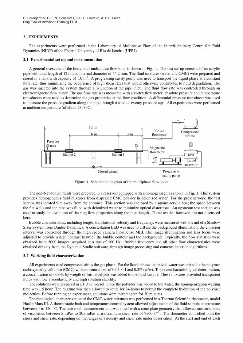
A general overview of the horizontal multiphase flow loop is shown in Fig. 1. The test set up consists of an acrylicpipe with total length of 12 m and internal diameter of 44.2 mm. The fluid mixtures (water and CMC) were prepared andstored in a tank with capacity of 1.0 m3. A progressing cavity pump was used to transport the liquid phase at a constantflow rate, thus minimizing the occurrence of high shear rates that would otherwise contributes to fluid degradation. Thegas was injected into the system through a T-junction at the pipe inlet. The fluid flow rate was controlled through anelectromagnetic flow meter. The gas flow rate was measured with a vortex flow meter; absolute pressure and temperaturetransducers were used to determine the gas properties at the flow condition. A differential pressure transducer was usedto measure the pressure gradient along the pipe through a total of twenty pressure taps. All experiments were performedat ambient temperature (of about 23.0 oC).

Liquidreservoir

Compressedair line

Vortexflowmeter

Pressuretaps

Closed circuit

Station 2 Station 1

6 m 3 m

12 m

Progressivecavity pump

Magnecticflowmeter

Figure 1. Schematic diagram of the multiphase flow loop.

The non-Newtonian fluids were prepared in a reservoir equipped with a homogenizer, as shown in Fig. 1. This systemprovides homogeneous fluid mixtures from dispersed CMC powder in deionized water. For the present work, the testsection was located 9 m away from the entrance. This section was enclosed by a square acrylic box; the space betweenthe flat walls and the pipe was filled with deionized water to minimize optical distortions. An upstream test section wasused to study the evolution of the slug flow properties along the pipe length. These results, however, are not discussedhere.

Bubble characteristics, including length, translational velocity and frequency, were measured with the aid of a ShadowSizer System from Dantec Dynamics. A constellation LED was used to diffuse the background illumination; the emissioninterval was controlled through the high speed camera FlowSense MIII. The image illumination and lens focus wereadjusted to provide a high contrast between the bubble contour and the background. Typically, the flow statistics wereobtained from 5000 images, acquired at a rate of 100 Hz. Bubble frequency and all other flow characteristics wereobtained directly from the Dynamic Studio software, through image processing and contour detection algorithms.

2.2 Working fluid characterization

All experiments used compressed air as the gas phase. For the liquid phase, deionized water was mixed to the polymercarboxymethylcellulose (CMC) with concentrations of 0.05, 0.1 and 0.2% (w/w). To prevent bacteriological deterioration,a concentration of 0.03% by weigth of formaldehyde was added to the fluid sample. These mixtures provided transparentfluids with low viscoelasticity and high solution stability.

The solutions were prepared in a 1.0 m3 vessel. Once the polymer was added to the water, the homogenization waitingtime was 1.5 hour. The mixture was then allowed to settle for 24 hours to permit the complete hydration of the polymermolecules. Before running an experiment, solutions were mixed again for 30 minutes.

The rheological characterization of the CMC-water mixtures was performed in a Thermo Scientific rheometer, modelHaake Mars III. A thermostatic bath and temperature control system allowed adjustments of the fluid sample temperaturebetween 4 to 120 oC. The universal measurement unit was fitted with a cone-plate geometry that allowed measurementsof viscosities between 5 mPas to 205 mPas at a maximum shear rate of 7500 s−1. The rheometer controlled both thestress and shear rate, depending on the ranges of viscosity and shear rate under observation. At the start and end of each


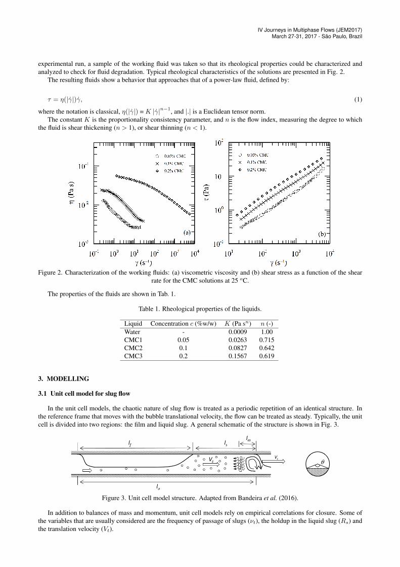
experimental run, a sample of the working fluid was taken so that its rheological properties could be characterized andanalyzed to check for fluid degradation. Typical rheological characteristics of the solutions are presented in Fig. 2.

The resulting fluids show a behavior that approaches that of a power-law fluid, defined by:

τ = η(|γ̇|)γ̇, (1)

where the notation is classical, η(|γ̇|) = K |γ̇|n−1, and |.| is a Euclidean tensor norm.The constant K is the proportionality consistency parameter, and n is the flow index, measuring the degree to which

the fluid is shear thickening (n > 1), or shear thinning (n < 1).

Figure 2. Characterization of the working fluids: (a) viscometric viscosity and (b) shear stress as a function of the shearrate for the CMC solutions at 25 oC.

The properties of the fluids are shown in Tab. 1.

Table 1. Rheological properties of the liquids.

Liquid Concentration c (%w/w) K (Pa sn) n (-)Water - 0.0009 1.00CMC1 0.05 0.0263 0.715CMC2 0.1 0.0827 0.642CMC3 0.2 0.1567 0.619

3. MODELLING

3.1 Unit cell model for slug flow

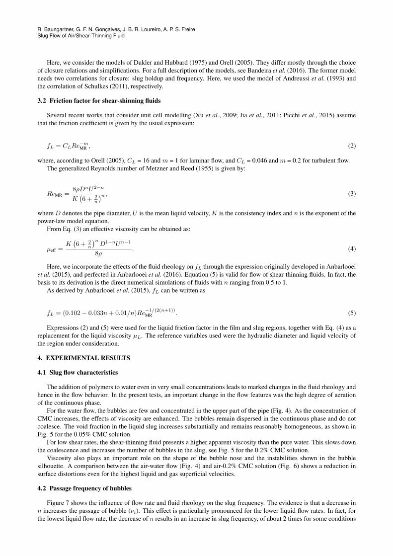
In the unit cell models, the chaotic nature of slug flow is treated as a periodic repetition of an identical structure. Inthe reference frame that moves with the bubble translational velocity, the flow can be treated as steady. Typically, the unitcell is divided into two regions: the film and liquid slug. A general schematic of the structure is shown in Fig. 3.

Figure 3. Unit cell model structure. Adapted from Bandeira et al. (2016).

In addition to balances of mass and momentum, unit cell models rely on empirical correlations for closure. Some ofthe variables that are usually considered are the frequency of passage of slugs (νt), the holdup in the liquid slug (Rs) andthe translation velocity (Vt).


Here, we consider the models of Dukler and Hubbard (1975) and Orell (2005). They differ mostly through the choiceof closure relations and simplifications. For a full description of the models, see Bandeira et al. (2016). The former modelneeds two correlations for closure: slug holdup and frequency. Here, we used the model of Andreussi et al. (1993) andthe correlation of Schulkes (2011), respectively.

3.2 Friction factor for shear-shinning fluids

Several recent works that consider unit cell modelling (Xu et al., 2009; Jia et al., 2011; Picchi et al., 2015) assumethat the friction coefficient is given by the usual expression:

fL = CLRe−mMR , (2)

where, according to Orell (2005), CL = 16 and m = 1 for laminar flow, and CL = 0.046 and m = 0.2 for turbulent flow.The generalized Reynolds number of Metzner and Reed (1955) is given by:

ReMR =8ρDnU2−n

K(6 + 2

n

)n , (3)

where D denotes the pipe diameter, U is the mean liquid velocity, K is the consistency index and n is the exponent of thepower-law model equation.

From Eq. (3) an effective viscosity can be obtained as:

µeff =K

(6 + 2

n

)nD1−nUn−1

8ρ. (4)

Here, we incorporate the effects of the fluid rheology on fL through the expression originally developed in Anbarlooeiet al. (2015), and perfected in Anbarlooei et al. (2016). Equation (5) is valid for flow of shear-thinning fluids. In fact, thebasis to its derivation is the direct numerical simulations of fluids with n ranging from 0.5 to 1.

As derived by Anbarlooei et al. (2015), fL can be written as

fL = (0.102− 0.033n+ 0.01/n)Re−1/(2(n+1))MR . (5)

Expressions (2) and (5) were used for the liquid friction factor in the film and slug regions, together with Eq. (4) as areplacement for the liquid viscosity µL. The reference variables used were the hydraulic diameter and liquid velocity ofthe region under consideration.

4. EXPERIMENTAL RESULTS

4.1 Slug flow characteristics

The addition of polymers to water even in very small concentrations leads to marked changes in the fluid rheology andhence in the flow behavior. In the present tests, an important change in the flow features was the high degree of aerationof the continuous phase.

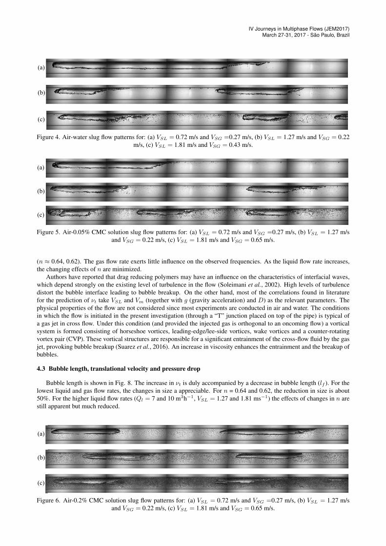
For the water flow, the bubbles are few and concentrated in the upper part of the pipe (Fig. 4). As the concentration ofCMC increases, the effects of viscosity are enhanced. The bubbles remain dispersed in the continuous phase and do notcoalesce. The void fraction in the liquid slug increases substantially and remains reasonably homogeneous, as shown inFig. 5 for the 0.05% CMC solution.

For low shear rates, the shear-thinning fluid presents a higher apparent viscosity than the pure water. This slows downthe coalescence and increases the number of bubbles in the slug, see Fig. 5 for the 0.2% CMC solution.

Viscosity also plays an important role on the shape of the bubble nose and the instabilities shown in the bubblesilhouette. A comparison between the air-water flow (Fig. 4) and air-0.2% CMC solution (Fig. 6) shows a reduction insurface distortions even for the highest liquid and gas superficial velocities.

4.2 Passage frequency of bubbles

Figure 7 shows the influence of flow rate and fluid rheology on the slug frequency. The evidence is that a decrease inn increases the passage of bubble (νt). This effect is particularly pronounced for the lower liquid flow rates. In fact, forthe lowest liquid flow rate, the decrease of n results in an increase in slug frequency, of about 2 times for some conditions


(a) (b)

(c) Figuair-w(a) $(b) $(c) $ for 0(d) $(e) $(f) $ for 0(g) $(h) $ (i) $ for (j) $(k) $(l) $

ure1: Bubblewater flows: $V_{SL}=$ $V_{SL}=$ $V_{SL}=$

0.05% CMC$V_{SL}=$ $V_{SL}=$ $V_{SL}=$

0.1% CMC-w$V_{SL}=$ $V_{SL}=$ $V_{SL}=$

0.2% CMC $V_{SL}=$ 0$V_{SL}=$ $V_{SL}=$ 1

e shaper for 0.72 m/s and1.27 m/s and1.81 m/s and

-water flows0.72 m/s and1.27 m/s and1.81 m/s and

water flows: 0.72 m/s and1.27 m/s and1.81 m/s and

flows: 0.72 m/s and1.27 m/s and1.81 m/s and

d $V_{SG}=d $V_{SG}=d $V_{SG}=

s: d $V_{SG}=d $V_{SG}=d $V_{SG}=



=0.27 m/s, =$ 0.22 m/s,=$ 0.43 m/s;

=$ 0.27 m/s,=$ 0.22 m/s, =$ 0.65 m/s;

=$ 0.27 m/s, =$ 0.22m/s, =$ 0.65 m/s,

$ 0.27 m/s, =$ 0.22 m/s,$ 0.65 m/s.

Figure 4. Air-water slug flow patterns for: (a) VSL = 0.72 m/s and VSG =0.27 m/s, (b) VSL = 1.27 m/s and VSG = 0.22m/s, (c) VSL = 1.81 m/s and VSG = 0.43 m/s.

(a)

(b)

(c) Figuair-w(a) $(b) $(c) $ for 0(d) $(e) $(f) $ for 0(g) $(h) $ (i) $ for (j) $(k) $(l) $


0.05% CMC$V_{SL}=$ $V_{SL}=$ $V_{SL}=$

0.1% CMC-w$V_{SL}=$ $V_{SL}=$ $V_{SL}=$

0.2% CMC $V_{SL}=$ 0$V_{SL}=$ $V_{SL}=$ 1

e shaper for 0.72 m/s and1.27 m/s and1.81 m/s and





s: d $V_{SG}=d $V_{SG}=d $V_{SG}=



=0.27 m/s, =$ 0.22 m/s,=$ 0.43 m/s;

=$ 0.27 m/s,=$ 0.22 m/s, =$ 0.65 m/s;

=$ 0.27 m/s, =$ 0.22m/s, =$ 0.65 m/s,

$ 0.27 m/s, =$ 0.22 m/s,$ 0.65 m/s.

Figure 5. Air-0.05% CMC solution slug flow patterns for: (a) VSL = 0.72 m/s and VSG =0.27 m/s, (b) VSL = 1.27 m/sand VSG = 0.22 m/s, (c) VSL = 1.81 m/s and VSG = 0.65 m/s.

(n ≈ 0.64, 0.62). The gas flow rate exerts little influence on the observed frequencies. As the liquid flow rate increases,the changing effects of n are minimized.

Authors have reported that drag reducing polymers may have an influence on the characteristics of interfacial waves,which depend strongly on the existing level of turbulence in the flow (Soleimani et al., 2002). High levels of turbulencedistort the bubble interface leading to bubble breakup. On the other hand, most of the correlations found in literaturefor the prediction of νt take VSL and Vm (together with g (gravity acceleration) and D) as the relevant parameters. Thephysical properties of the flow are not considered since most experiments are conducted in air and water. The conditionsin which the flow is initiated in the present investigation (through a “T” junction placed on top of the pipe) is typical ofa gas jet in cross flow. Under this condition (and provided the injected gas is orthogonal to an oncoming flow) a vorticalsystem is formed consisting of horseshoe vortices, leading-edge/lee-side vortices, wake vortices and a counter-rotatingvortex pair (CVP). These vortical structures are responsible for a significant entrainment of the cross-flow fluid by the gasjet, provoking bubble breakup (Suarez et al., 2016). An increase in viscosity enhances the entrainment and the breakup ofbubbles.

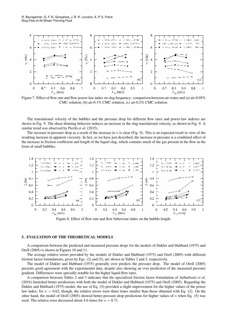
4.3 Bubble length, translational velocity and pressure drop

Bubble length is shown in Fig. 8. The increase in νt is duly accompanied by a decrease in bubble length (lf ). For thelowest liquid and gas flow rates, the changes in size a appreciable. For n = 0.64 and 0.62, the reduction in size is about50%. For the higher liquid flow rates (Ql = 7 and 10 m3h−1, VSL = 1.27 and 1.81 ms−1) the effects of changes in n arestill apparent but much reduced.

(a)

(b) (c) Figuair-w(a) $(b) $(c) $ for 0(d) $(e) $(f) $ for 0(g) $(h) $ (i) $ for (j) $(k) $(l) $


0.05% CMC$V_{SL}=$ $V_{SL}=$ $V_{SL}=$

0.1% CMC-w$V_{SL}=$ $V_{SL}=$ $V_{SL}=$

0.2% CMC $V_{SL}=$ 0$V_{SL}=$ $V_{SL}=$ 1

e shapes for 0.72 m/s and1.27 m/s and1.81 m/s and





s: d $V_{SG}=d $V_{SG}=d $V_{SG}=



=0.27 m/s, =$ 0.22 m/s,=$ 0.43 m/s;

=$ 0.27 m/s,=$ 0.22 m/s, =$ 0.65 m/s;

=$ 0.27 m/s, =$ 0.22m/s, =$ 0.65 m/s,

$ 0.27 m/s, =$ 0.22 m/s,$ 0.65 m/s.

Figure 6. Air-0.2% CMC solution slug flow patterns for: (a) VSL = 0.72 m/s and VSG =0.27 m/s, (b) VSL = 1.27 m/sand VSG = 0.22 m/s, (c) VSL = 1.81 m/s and VSG = 0.65 m/s.


Figure 7. Effect of flow rate and flow power-law index on slug frequency: comparison between air-water and (a) air-0.05%CMC solution, (b) air-0.1% CMC solution, (c) air-0.2% CMC solution.

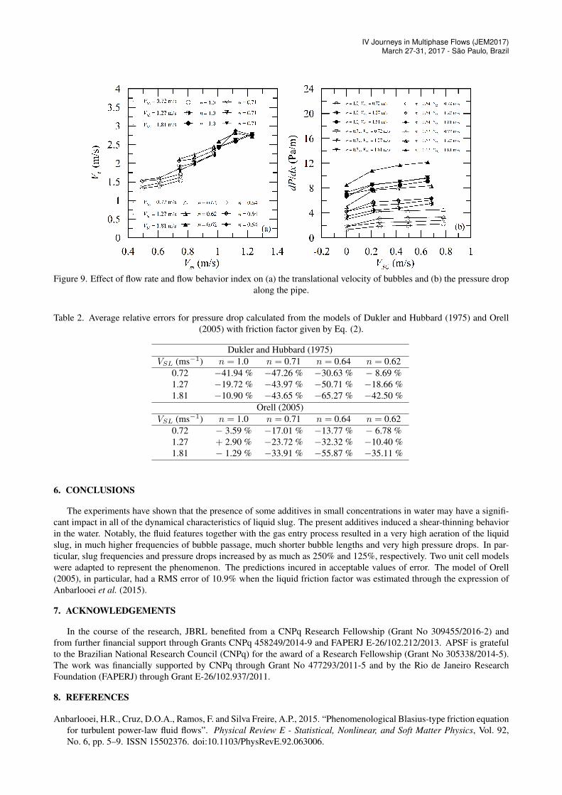
The translational velocity of the bubbles and the pressure drop for different flow rates and power-law indexes areshown in Fig. 9. The shear-thinning behavior induces an increase in the slug translational velocity, as shown in Fig. 9. Asimilar trend was observed by Picchi et al. (2015).

The increase in pressure drop as a result of the increase in n is clear (Fig. 9). This is an expected result in view of theresulting increase in apparent viscosity. In fact, as we have just described, the increase in pressure is a combined effect ofthe increase in friction coefficient and length of the liquid slug, which contains much of the gas present in the flow in theform of small bubbles.

Figure 8. Effect of flow rate and flow behaviour index on the bubble length.

5. EVALUATION OF THE THEORETICAL MODELS

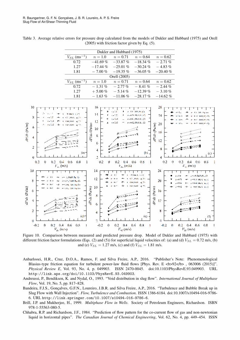
A comparison between the predicted and measured pressure drops for the models of Dukler and Hubbard (1975) andOrell (2005) is shown in Figures 10 and 11.

The average relative errors provided by the models of Dukler and Hubbard (1975) and Orell (2005) with differentfriction factor formulations, given by Eqs. (2) and (5), are shown in Tables 2 and 3, respectively.

The model of Dukler and Hubbard (1975) generally over predicts the pressure drop. The model of Orell (2005)presents good agreement with the experimental data, despite also showing an over prediction of the measured pressuregradient. Differences were specially notable for the higher liquid flow rates.

A comparison between Tables 2 and 3 indicates that the specialized friction factor formulation of Anbarlooei et al.(2016) furnished better predictions with both the model of Dukler and Hubbard (1975) and Orell (2005). Regarding theDukler and Hubbard (1975) model, the use of Eq. (5) provided a slight improvement for the higher values of the powerlaw index; for n = 0.62, though, the relative errors were three times smaller than those obtained with Eq. (2). On theother hand, the model of Orell (2005) showed better pressure drop predictions for higher values of n when Eq. (5) wasused. The relative error decreased about 4.6 times for n = 0.71.


Figure 9. Effect of flow rate and flow behavior index on (a) the translational velocity of bubbles and (b) the pressure dropalong the pipe.

Table 2. Average relative errors for pressure drop calculated from the models of Dukler and Hubbard (1975) and Orell(2005) with friction factor given by Eq. (2).

Dukler and Hubbard (1975)VSL (ms−1) n = 1.0 n = 0.71 n = 0.64 n = 0.62

0.72 −41.94 % −47.26 % −30.63 % − 8.69 %1.27 −19.72 % −43.97 % −50.71 % −18.66 %1.81 −10.90 % −43.65 % −65.27 % −42.50 %

Orell (2005)VSL (ms−1) n = 1.0 n = 0.71 n = 0.64 n = 0.62

0.72 − 3.59 % −17.01 % −13.77 % − 6.78 %1.27 + 2.90 % −23.72 % −32.32 % −10.40 %1.81 − 1.29 % −33.91 % −55.87 % −35.11 %

6. CONCLUSIONS

The experiments have shown that the presence of some additives in small concentrations in water may have a signifi-cant impact in all of the dynamical characteristics of liquid slug. The present additives induced a shear-thinning behaviorin the water. Notably, the fluid features together with the gas entry process resulted in a very high aeration of the liquidslug, in much higher frequencies of bubble passage, much shorter bubble lengths and very high pressure drops. In par-ticular, slug frequencies and pressure drops increased by as much as 250% and 125%, respectively. Two unit cell modelswere adapted to represent the phenomenon. The predictions incured in acceptable values of error. The model of Orell(2005), in particular, had a RMS error of 10.9% when the liquid friction factor was estimated through the expression ofAnbarlooei et al. (2015).

7. ACKNOWLEDGEMENTS

In the course of the research, JBRL benefited from a CNPq Research Fellowship (Grant No 309455/2016-2) andfrom further financial support through Grants CNPq 458249/2014-9 and FAPERJ E-26/102.212/2013. APSF is gratefulto the Brazilian National Research Council (CNPq) for the award of a Research Fellowship (Grant No 305338/2014-5).The work was financially supported by CNPq through Grant No 477293/2011-5 and by the Rio de Janeiro ResearchFoundation (FAPERJ) through Grant E-26/102.937/2011.

8. REFERENCES

Anbarlooei, H.R., Cruz, D.O.A., Ramos, F. and Silva Freire, A.P., 2015. “Phenomenological Blasius-type friction equationfor turbulent power-law fluid flows”. Physical Review E - Statistical, Nonlinear, and Soft Matter Physics, Vol. 92,No. 6, pp. 5–9. ISSN 15502376. doi:10.1103/PhysRevE.92.063006.


Table 3. Average relative errors for pressure drop calculated from the models of Dukler and Hubbard (1975) and Orell(2005) with friction factor given by Eq. (5).

Dukler and Hubbard (1975)VSL (ms−1) n = 1.0 n = 0.71 n = 0.64 n = 0.62

0.72 −41.69 % −33.87 % −18.34 % − 2.71 %1.27 −17.44 % −25.01 % −30.24 % − 4.83 %1.81 − 7.00 % −19.35 % −36.05 % −20.40 %

Orell (2005)VSL (ms−1) n = 1.0 n = 0.71 n = 0.64 n = 0.62

0.72 − 1.31 % − 2.77 % − 8.41 % − 2.44 %1.27 + 5.00 % − 5.14 % −12.39 % − 3.10 %1.81 − 1.63 % −11.06 % −28.17 % −14.62 %

Figure 10. Comparison between measured and predicted pressure drop. Model of Dukler and Hubbard (1975) withdifferent friction factor formulations (Eqs. (2) and (5)) for superficial liquid velocities of: (a) and (d) VSL = 0.72 m/s, (b)

and (e) VSL = 1.27 m/s, (c) and (f) VSL = 1.81 m/s.

Anbarlooei, H.R., Cruz, D.O.A., Ramos, F. and Silva Freire, A.P., 2016. “Publisher’s Note: PhenomenologicalBlasius-type friction equation for turbulent power-law fluid flows [Phys. Rev. E <b>92</b> , 063006 (2015)]”.Physical Review E, Vol. 93, No. 4, p. 049903. ISSN 2470-0045. doi:10.1103/PhysRevE.93.049903. URLhttp://link.aps.org/doi/10.1103/PhysRevE.93.049903.

Andreussi, P., Bendiksen, K. and Nydal, O., 1993. “Void distribution in slug flow”. International Journal of MultiphaseFlow, Vol. 19, No. 5, pp. 817–828.

Bandeira, F.J.S., Gonçalves, G.F.N., Loureiro, J.B.R. and Silva Freire, A.P., 2016. “Turbulence and Bubble Break up inSlug Flow with Wall Injection”. Flow, Turbulence and Combustion. ISSN 1386-6184. doi:10.1007/s10494-016-9786-6. URL http://link.springer.com/10.1007/s10494-016-9786-6.

Brill, J.P. and Mukherjee, H., 1999. Multiphase Flow in Wells. Society of Petroleum Engineers, Richardson. ISBN978-1-55563-080-5.

Chhabra, R.P. and Richardson, J.F., 1984. “Prediction of flow pattern for the co-current flow of gas and non-newtonianliquid in horizontal pipes”. The Canadian Journal of Chemical Engineering, Vol. 62, No. 4, pp. 449–454. ISSN


Figure 11. Comparison between measured and predicted pressure drop. Model of Orell (2005) with different frictionfactor formulations (Eqs. (2) and (5)) for superficial liquid velocities of: (a) and (d) VSL = 0.72 m/s, (b) and (e) VSL =

1.27 m/s, (c) and (f) VSL = 1.81 m/s.

00084034.Dukler, A. and Hubbard, M., 1975. “A model for gas-liquid slug flow in horizontal and near horizon-

tal tubes”. Industrial & Engineering Chemistry Fundamentals, Vol. 14, No. 4, pp. 337–347. URLhttp://pubs.acs.org/doi/abs/10.1021/i160056a011.

Jia, N., Gourma, M. and Thompson, C.P., 2011. “Non-Newtonian multi-phase flows: On drag reduction, pressure dropand liquid wall friction factor”. Chemical Engineering Science, Vol. 66, No. 20, pp. 4742–4756. ISSN 00092509.doi:10.1016/j.ces.2011.06.067. URL http://dx.doi.org/10.1016/j.ces.2011.06.067.

Metzner, A.B. and Reed, J., 1955. “Flow of Non-Newtonian Fluids – Correlation of the Laminar, Transition and Turbulent-flow regions”. A.I.Ch.E. Journal, Vol. 1, p. 434.

Orell, A., 2005. “Experimental validation of a simple model for gas liquid slug flow in horizontal pipes”. Chemi-cal Engineering Science, Vol. 60, No. 5, pp. 1371–1381. ISSN 00092509. doi:10.1016/j.ces.2004.09.082. URLhttp://linkinghub.elsevier.com/retrieve/pii/S000925090400778X.

Otten, L. and Fayed, A.S., 1976. “Pressure drop and drag reduction in two-phase non-newtonian slug flow”. The CanadianJournal of Chemical Engineering, Vol. 54, No. 1-2, pp. 111–114. ISSN 00084034. doi:10.1002/cjce.5450540117.URL http://doi.wiley.com/10.1002/cjce.5450540117.

Picchi, D., Manerba, Y., Correra, S., Margarone, M. and Poesio, P., 2015. “Gas/shear-thinningliquid flows through pipes: Modeling and experiments”. International Journal of MultiphaseFlow, Vol. 73, pp. 217–226. ISSN 03019322. doi:10.1016/j.ijmultiphaseflow.2015.03.005. URLhttp://dx.doi.org/10.1016/j.ijmultiphaseflow.2015.03.005.

Rosehart, R.G., Rhodes, E. and Scott, D.S., 1975. “Studies of gas-liquid (non-Newtonian) slug flow: void fraction meter,void fraction and slug characteristics”. The Chemical Engineering Journal, Vol. 10, No. 1, pp. 57–64. ISSN 03009467.doi:10.1016/0300-9467(75)88017-8.

Schulkes, R., 2011. “Slug Frequencies Revisited”. 15th International Conference on Multiphase Production Technology,, No. 1969, pp. 311–325.

Soleimani, A., Al-Sarkhi, A. and Hanratty, T.J., 2002. “Effect of drag-reducing polymers on pseudo-slugs - Interfacialdrag and transition to slug flow”. International Journal of Multiphase Flow, Vol. 28, No. 12, pp. 1911–1927. ISSN03019322. doi:10.1016/S0301-9322(02)00110-6.


Suarez, A., Loureiro, J. and Silva Freire, A., 2016. “Characterization of Inclined Gas Jets in Two-Phase Crossflow”. In16th Brazilian Congress of Thermal Sciences and Engineering. 1993.

Xu, J.y., Wu, Y.x., Li, H., Guo, J. and Chang, Y., 2009. “Study of drag reduction by gas injection for power-law fluid flowin horizontal stratified and slug flow regimes”. Chemical Engineering Journal, Vol. 147, No. 2-3, pp. 235–244. ISSN13858947. doi:10.1016/j.cej.2008.07.006.

9. RESPONSIBILITY NOTICE

The authors are the only responsible for the printed material included in this paper.

Documents

HORIZONTAL PIPE SLUG FLOW OF AIR/SHEAR-THINNING …eventos.abcm.org.br/jem2017/content/uploads/2017/03/JEM-2017-0053… · R. Baungartner, G. F. N. Gonçalves, J. B. R. Loureiro,