Embed Size (px)
Citation preview
HOOK FORMULAS FOR SKEW SHAPES
ALEJANDRO H. MORALES?, IGOR PAK?, AND GRETA PANOVA†
Abstract. The celebrated hook-length formula gives a product formula for the number of standardYoung tableaux of a straight shape. In 2014, Naruse announced a more general formula for the number
of standard Young tableaux of skew shapes as a positive sum over excited diagrams of products of
hook-lengths. We give an algebraic and a combinatorial proof of Naruse’s formula, by using factorialSchur functions and a generalization of the Hillman-Grassl correspondence, respectively.
The main new results are two different q-analogues of Naruse’s formula: for the skew Schur
functions, and for counting reverse plane partitions of skew shapes. We establish explicit bijectionsbetween these objects and families of integer arrays with certain nonzero entries, which also proves
the second formula. We then apply our results to border strip shapes and their generalizations. In
particular, we obtain curious new formulas for the Euler and q-Euler numbers in terms of certainDyck path summations.
1. Introduction
1.1. Foreword. The classical hook-length formula (HLF) for the number of standard Young tableaux(SYT) of a Young diagram, is a beautiful result in enumerative combinatorics that is both mysteriousand extremely well studied. In a way it is a perfect formula – highly nontrivial, clean, concise andgeneralizing several others (binomial coefficients, Catalan numbers, etc.) The HLF was discoveredby Frame, Robinson and Thrall [FRT] in 1954, and by now it has numerous proofs: probabilistic,bijective, inductive, analytic, geometric, etc. (see §11.2). Arguably, each of these proofs does not reallyexplain the HLF on a deeper level, but rather tells a different story, leading to new generalizationsand interesting connections to other areas. In this paper we prove a new generalization of the HLFfor skew shapes which presented an unusual and interesting challenge; it has yet to be fully explainedand understood.
For skew shapes, there is no product formula for the number fλ/µ of standard Young tableaux(cf. Section 10). Most recently, in the context of equivariant Schubert calculus, Naruse presentedand outlined a proof in [Naru] of a remarkable generalization on the HLF, which we call the Narusehook-length formula (NHLF). This formula (see below), writes fλ/µ as a sum of “hook products” overthe excited diagrams, defined as certain generalizations of skew shapes. These excited diagrams wereintroduced by Ikeda and Naruse [IN1], and in a slightly different form independently by Kreiman [Kre1,Kre2] and Knutson, Miller and Yong [KMY]. They are a combinatorial model for the terms appearingin the formula for Kostant polynomials discovered independently by Andersen–Jantzen–Soergel [AJS,Appendix D] and Billey [Bil] (see Remark 4.2 and §11.3). These diagrams are the main combinatorialobjects in this paper and have difficult structure even in nice special cases (cf. § 8.1).
The goals of this paper are threefold. First, we give Naruse-style hook formulas for the Schurfunction sλ/µ(1, q, q2, . . .), which is the generating function for semistandard Young tableaux (SSYT)of shape λ/µ, and for the generating function for reverse plane partitions (RPP) of the same shape.Both can be viewed as q-analogues of NHLF. In contrast with the case of straight shapes, here these
Key words and phrases. Hook-length formula, excited tableau, standard Young tableau, flagged tableau, reverse plane
partition, Hillman-Grassl correspondence, Robinson-Schensted-Knuth correspondence, Greene’s theorem, alternating
permutation, Dyck path, Euler numbers, Catalan numbers, Grassmannian permutation, factorial Schur function.June 28, 2016.?Department of Mathematics, UCLA, Los Angeles, CA 90095. Email: ahmorales,[email protected].†Department of Mathematics, UPenn, Philadelphia, PA 19104. Email: [email protected].
1
2 ALEJANDRO MORALES, IGOR PAK, GRETA PANOVA
two formulas are quite different. Even the summations are over different sets – in the case of RPPwe sum over pleasant diagrams which we introduce. The proofs employ a combination of algebraicand bijective arguments, using the factorial Schur functions and the Hillman-Grassl correspondence,respectively. While the algebraic proof uses some powerful known results, the bijective proof is veryinvolved and occupies much of the paper.
Second, as a biproduct of our proofs we give the first purely combinatorial (but non-bijective) proofof Naruse’s formula. We also obtain trace generating functions for both SSYT and RPP of skewshape, simultaneously generalizing classical Stanley and Gansner formulas, and our q-analogues. Wealso investigate combinatorics of excited and pleasant diagrams and how they related to each other,which allow us simplify the RPP case.
Third, we apply our results to the case of border strips δm+2/δm and more general thick stripsδm+2k/δm. We obtain new summation formulas for two different q-Euler polynomials and a host ofdeterminant formulas.
1.2. Hook formulas for straight and skew shapes. We assume here the reader is familiar withthe basic definitions, which are postponed until the next two sections.
The standard Young tableaux (SYT) of straight and skew shapes are central objects in enumerativeand algebraic combinatorics. The number fλ = |SYT(λ)| of standard Young tableaux of shape λ hasthe celebrated hook-length formula (HLF):
Theorem 1.1 (HLF; Frame–Robinson–Thrall [FRT]). Let λ be a partition of n. We have:
(1.1) fλ =n!∏
u∈[λ] h(u),
where h(u) = λi − i+ λ′j − j + 1 is the hook-length of the square u = (i, j).
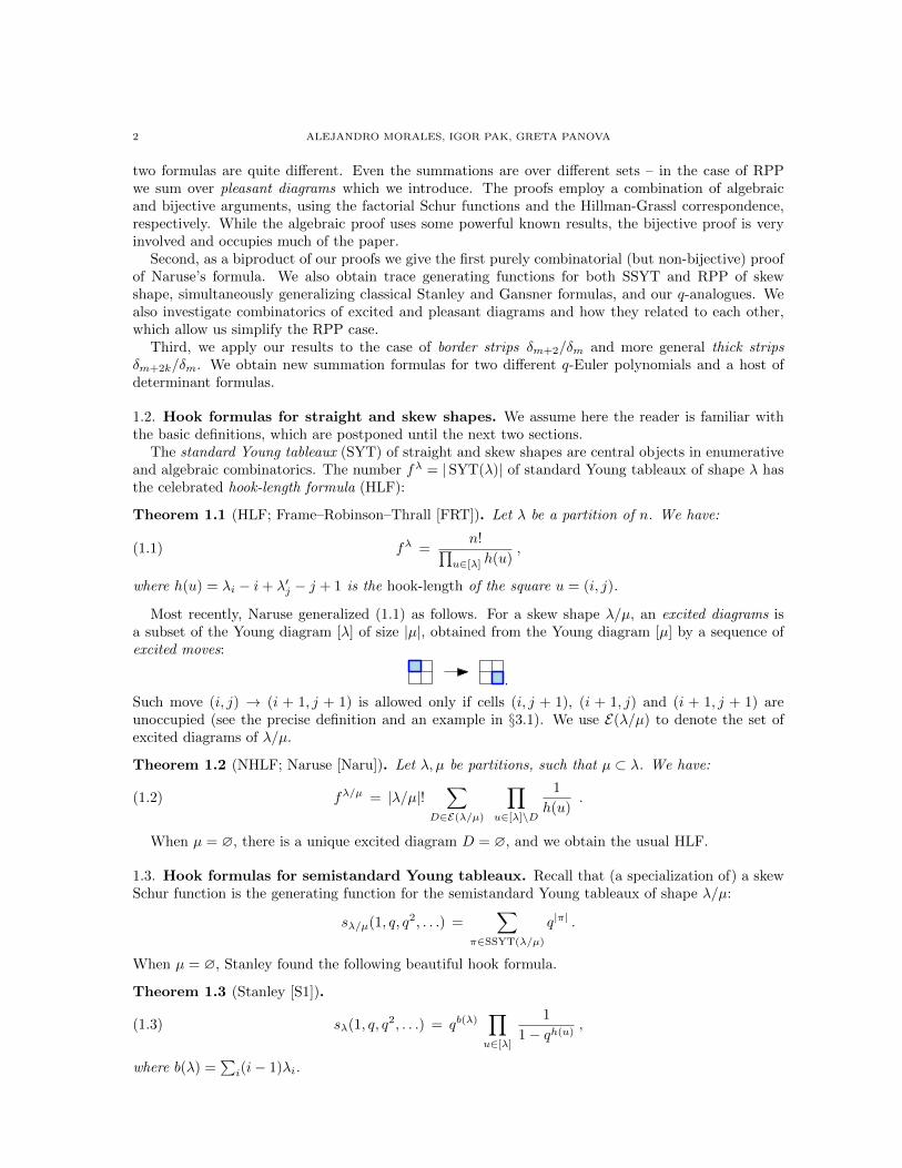
Most recently, Naruse generalized (1.1) as follows. For a skew shape λ/µ, an excited diagrams isa subset of the Young diagram [λ] of size |µ|, obtained from the Young diagram [µ] by a sequence ofexcited moves:
.
Such move (i, j) → (i + 1, j + 1) is allowed only if cells (i, j + 1), (i + 1, j) and (i + 1, j + 1) areunoccupied (see the precise definition and an example in §3.1). We use E(λ/µ) to denote the set ofexcited diagrams of λ/µ.
Theorem 1.2 (NHLF; Naruse [Naru]). Let λ, µ be partitions, such that µ ⊂ λ. We have:
(1.2) fλ/µ = |λ/µ|!∑
D∈E(λ/µ)
∏u∈[λ]\D
1
h(u).
When µ = ∅, there is a unique excited diagram D = ∅, and we obtain the usual HLF.
1.3. Hook formulas for semistandard Young tableaux. Recall that (a specialization of) a skewSchur function is the generating function for the semistandard Young tableaux of shape λ/µ:
sλ/µ(1, q, q2, . . .) =∑
π∈SSYT(λ/µ)
q|π| .
When µ = ∅, Stanley found the following beautiful hook formula.
Theorem 1.3 (Stanley [S1]).
(1.3) sλ(1, q, q2, . . .) = qb(λ)∏u∈[λ]
1
1− qh(u),
where b(λ) =∑i(i− 1)λi.
HOOK FORMULAS FOR SKEW SHAPES 3
This formula can be viewed as q-analogue of the HLF. In fact, one can derive HLF (1.1) from (1.3)by Stanley’s theory of P -partitions [S3, Prop. 7.19.11] or by a geometric argument [Pak, Lemma 1].Here we give the following natural analogue of NHLF (1.3).
Theorem 1.4. We have:
(1.4) sλ/µ(1, q, q2, . . .) =∑
S∈E(λ/µ)
∏(i,j)∈[λ]\S
qλ′j−i
1− qh(i,j).
By analogy with the straight shape, Theorem 1.4 implies NHLF, see Proposition 3.4. We proveTheorem 1.4 in Section 4 by using algebraic tools.
1.4. Hook formulas for reverse plane partitions via bijections. In the case of staight shapes,the enumeration of RPP can be obtained from SSYT, by subtracting (i − 1) from the entries in thei-th row. In other words, we have:
(1.5)∑
π∈RPP(λ)
q|π| =∏u∈[λ]
1
1− qh(u).
Note that the above relation does not hold for skew shapes, since entries on the i-th row of a skewSSYT do not have to be at least (i− 1).
Formula (1.5) has a classical combinatorial proof by the Hillman-Grassl correspondence [HiG], whichgives a bijection Φ between RPP ranked by the size and nonnegative arrays of shape λ ranked by thehook weight. We view RPP of skew shape λ/µ as a special case of RPP of shape λ. The major technicalresult of the paper is Theorem 7.7, which states that the restriction of Φ gives a bijection betweenSSYT of shape λ/µ and arrays of nonnegative integers of shape λ with zeroes in the excited diagramand certain nonzero cells (excited arrays, see Definition 7.1). In other words, we fully characterize thepreimage of the SSYT of shape λ/µ under the map Φ. This and the properties of Φ allows us to obtaina number of generalizations of Theorem 1.4 (see below).
The proof of Theorem 7.7 goes through several steps of interpretations using careful analysis oflongest decreasing subsequences in these arrays and a detailed study of structure of the resultingtableaux under RSK. We built on top of the celebrated Greene’s theorem and several Gansner’s results.As a corollary of our proof of Theorem 7.7, we obtain the following generalization of formula (1.5).This result is natural from enumerative point of view, but is unusual in the literature (cf. Section 10and §11.5), and is completely independent of Theorem 1.4.
Theorem 1.5. We have:
(1.6)∑
π∈RPP(λ/µ)
q|π| =∑
S∈P(λ/µ)
∏u∈S
qh(u)
1− qh(u),
where P(λ/µ) is the set of pleasant diagrams (see Definition 6.1 ).
The theorem employs a new family of combinatorial objects called pleasant diagrams. These di-agrams can be defined as subsets of complements of excited diagrams (see Theorem 6.10), and aretechnically useful. This allows us to write the RHS of (1.6) completely in terms of excited diagrams(see Corollary 6.17). Note also that as corollary of Theorem 1.5, we obtain a combinatorial proof ofNHLF (see §6.4).
1.5. Further extensions. One of the most celebrated formula in enumerative combinatorics is MacMa-hon’s formula for enumeration of plane partitions, which can be viewed as a limit case of Stanley’strace formula (see [S1, S2]):∑
π∈PP
q|π| =
∞∏n=1
1
(1− qn)n,
∑π∈PP(m`)
q|π| ttr(π) =
m∏i=1
∏j=1
1
1− tqi+j−1.
Here tr(π) refers to the trace of the plane partition.
4 ALEJANDRO MORALES, IGOR PAK, GRETA PANOVA
These results were further generalized by Gansner [G1] by using the properties of the Hillman-Grasslcorrespondence combined with that of the RSK correspondence (cf. [G2]).
Theorem 1.6 (Gansner [G1]). We have:
(1.7)∑
π∈RPP(λ)
q|π| ttr(π) =∏u∈λ
1
1− tqh(u)
∏u∈[λ]\λ
1
1− qh(u),
where λ is the Durfee square of the Young diagram of λ.
For SSYT and RPP of skew shapes, our analysis of the Hillman-Grassl correspondence gives thefollowing simultaneous generalizations of Gansner’s theorem and our theorems 1.4 and 1.5.
Theorem 1.7. We have:
(1.8)∑
π∈RPP(λ/µ)
q|π| ttr(π) =∑
S∈P(λ/µ)
∏u∈S∩λ
tqh(u)
1− tqh(u)
∏u∈S\λ
qh(u)
1− qh(u).
As with the (1.5), the RHS of (1.8) can be stated completely in terms of excited diagrams (seeCorollary 6.19).
Theorem 1.8. We have:
(1.9)∑
π∈SSYT(λ/µ)
q|π| ttr(π) =∑
S∈E(λ/µ)
qa(S) tc(S)∏
u∈S∩λ
1
1− tqh(u)
∏u∈S\λ
1
1− qh(u),
where S = [λ] \ S, a(S) =∑
(i,j)∈[λ]\S(λ′j − i) and c(S) = |supp(AS)∩λ| is the size of the support of
the excited array AS inside the Durfee square λ of λ.
Let us emphasize that the proof Theorem 1.8 requires both the algebraic proof of Theorem 1.4 andthe analysis of the Hillman-Grassl correspondence.
1.6. Enumerative applications. In sections 8 and 9, we give enumerative formulas which followfrom NHLF. They involve q-analogues of Catalan, Euler and Schroder numbers. We highlight severalof these formulas.
Let Alt(n) = σ(1) < σ(2) > σ(3) < σ(4) > . . . ⊂ Sn be the set of alternating permutations. Thenumber En = |Alt(n)| is the n-th Euler number (see [S5] and [OEIS, A000111]), with the g.f.
(1.10) 1 +
∞∑n=1
Enzn
n!= tan(z) + sec(z) .
Let δn = (n−1, n−2, . . . , 2, 1) denotes the staircase shape and observe that E2n+1 = fδn+2/δn . Thus,the NHLF relates Euler numbers with excited diagrams of δn+2/δn. It turns out that these exciteddiagrams are in correspondence with the set Dyck(n) of Dyck paths of length 2n (see Proposition 8.1).More precisely,
|E(δn+2/δn)| = |Dyck(n)| = Cn =1
n+ 1
(2n
n
),
where Cn is the n-th Catalan number, and Dyck(n) is the set of lattice paths from (0, 0) to (2n, 0)with steps (1, 1) and (1,−1) that stay on or above the x-axis (see e.g. [S6]). Now the NHLF impliesthe following identity.
Corollary 1.9. We have:
(1.11)∑
γ∈Dyck(n)
∏(a,b)∈γ
1
2b+ 1=
E2n+1
(2n+ 1)!,
where (a, b) ∈ γ denotes a point (a, b) of the Dyck path γ.
HOOK FORMULAS FOR SKEW SHAPES 5
Consider the following two q-analogues of En :
En(q) :=∑
σ∈Alt(n)
qmaj(σ−1) and E∗n(q) :=∑
σ∈Alt(n)
qmaj(σ−1κ) ,
where maj(σ) is the major index of permutation σ in Sn and κ is the permutation κ = (13254 . . .).See examples 8.6 and 9.4 for the initial values.
Now, for the skew shape δn+2/δn, Theorem 1.4 gives the following q-analogue of Corollary 1.9.
Corollary 1.10. We have:∑γ∈Dyck(n)
∏(a,b)∈γ
qb
1− q2b+1=
E2n+1(q)
(1− q)(1− q2) · · · (1− q2n+1).
Similarly, Theorem 1.5 in this case gives a different q-analogue.
Corollary 1.11. We have:∑γ∈Dyck(n)
qH(γ)∏
(a,b)∈γ
1
1− q2b+1=
E∗2n+1(q)
(1− q)(1− q2) · · · (1− q2n+1),
where
H(γ) =∑
(c,d)∈HP(γ)
(2d+ 1) ,
and HP(γ) denotes the set of peaks (c, d) in γ with height d > 1.
All three corollaries are derived in sections 8 and 9.
1.7. Comparison with other formulas. In Section 10 we provide a comprehensive overview of theother formulas for fλ/µ that are either already present in the literature or could be deduced. We showthat the NHLF is not a restatement of any of them, and in particular demonstrate how it differs inthe number of summands and the terms themselves.
The classical formulas are the Jacobi-Trudi identity, which has negative terms, and the expansionof fλ/µ via the Littlewood–Richardson rule as a sum over fν for ν ` n. Another formula is theOkounkov–Olshanski identity summing particular products over SSYTs of shape µ. While it lookssimilar to the NHLF, it has more terms and the products are not over hook-lengths.
We outline another approach to formulas for fλ/µ. We observe that the original proof of Naruse ofthe NHLF in [Naru] comes from a particular specialization of the formal variables in the evaluation ofequivariant Schubert structure constants (generalized Littlewood–Richardson coefficients) correspond-ing to Grassmannian permutations. Ikeda-Naruse give a formula for their evaluation in [IN1] via theexcited diagrams on one-hand and an iteration of a Chevalley formula on the other hand, which givesthe correspondence with skew standard Young tableaux. Our algebraic proof of Theorem 1.3 followsthis approach.
Now, there are other expressions for these equivariant Schubert structure constants, which via theabove specialization would give enumerative formulas for fλ/µ. First, the Knutson-Tao puzzles [KT]give an enumerative formula as a sum over puzzles of a product of weights corresponding to it. Asshown in [MPP] this formula is equivalent to the Okounkov–Olshanski formula and hence differentfrom the sum over excited diagrams. Yet another rule for the evaluation of these specific structureconstants is given by Thomas and Yong in [TY], as a sum over certain edge-labeled skew SYTs ofproducts of weights (corresponding to the edge label’s paths under jeu-de-taquin). An example inSection 10 illustrates that the terms in the formula are different from the terms in the NHLF.
6 ALEJANDRO MORALES, IGOR PAK, GRETA PANOVA
1.8. Paper outline. The rest of the paper is organized as follows. We begin with notation, basicdefinitions and background results (Section 2). The definition of excited diagrams is given in Section 3,together with the original formula of Naruse and corollaries of the q-analogue. It also contains theenumerative properties of excited diagrams and the correspondence with flagged tableaux. In Sec-tion 4, we give an algebraic proof of the main Theorem 1.4. Section 7 described the Hillman-Grasslcorrespondence, with various properties and an equivalent formulation using the RSK correspondencein Corollary 5.8.
Section 6 defines pleasant diagrams and proves Theorem 1.5 using the Hillman-Grassl correspon-dence, and as a corollary gives a purely combinatorial proof of NHLF (Theorem 1.2). Then, inSection 7, we show that the Hillman-Grassl map is a bijection between skew SSYT of shape λ/µ andcertain integer arrays whose support is in the complement of an excited diagram. Section 8 considersthe special case when λ/µ is a thick strip shape, which give the connection with Euler and Catalannumbers.
In Section 9, we consider the pleasant diagrams of the thick strip shapes, establishing connectionwith Schroder numbers. We also state conjectures on certain determinantal formulas. Section 10compares NHLF and other formulas for fλ/µ. We conclude with final remarks and open problems inSection 11.
2. Notation and definitions
2.1. Young diagrams. Let λ = (λ1, . . . , λr), µ = (µ1, . . . , µs) denote integer partitions of length`(λ) = r and `(µ) = s. The size of the partition is denoted by |λ| and λ′ denotes the conjugate partitionof λ. We use [λ] to denote the Young diagram of the partition λ. The hook length hij = λi−i+λ′j−j+1of a square u = (i, j) ∈ [λ] is the number of squares directly to the right and directly below u in [λ].The Durfee square λ is the largest square inside [λ]; it is always of the form (i, j), 1 ≤ i, j ≤ k.
A skew shape is denoted by λ/µ. For an integer k, 1 − `(λ) ≤ k ≤ λ1 − 1, let dk be the diagonal(i, j) ∈ λ/µ | i− j = k, where µk = 0 if k > `(µ). For an integer t, 1 ≤ t ≤ `(λ)− 1 let dt(µ) denotethe diagonal dµt−t where µt = 0 if `(µ) < t ≤ `(λ).
Given the skew shape λ/µ, let Pλ/µ be the poset of cells (i, j) of [λ/µ] partially ordered by compo-nent. This poset is naturally labelled, unless otherwise stated.
2.2. Young tableaux. A reverse plane partition of skew shape λ/µ is an array π = (πij) of non-negative integers of shape λ/µ that is weakly increasing in rows and columns. We denote the set ofsuch plane partitions by RPP(λ/µ). A semistandard Young tableau of shape λ/µ is a RPP of shapeλ/µ that is strictly increasing in columns. We denote the set of such tableaux by SSYT(λ/µ). Astandard Young tableau (SYT) of shape λ/µ is an array T of shape λ/µ with the numbers 1, . . . , n,where n = |λ/µ|, each i appearing once, strictly increasing in rows and columns. For example, thereare five SYT of shape (32/1):
1 23 4
1 32 4
1 42 3
2 31 4
2 41 3
The size of a RPP or tableau T is the sum of its entries. A descent of a SYT T is an index i such thati+ 1 appears in a row below i. The major index tmaj(T ) is the sum
∑i over all the descents of T .
2.3. Symmetric functions. Let sλ/µ(x) denote the skew Schur function of shape λ/µ in variablesx = (x0, x1, x2, . . .). In particular,
sλ/µ(x) =∑
T∈SSYT(λ/µ)
xT , sλ/µ(1, q, q2, . . .) =∑
T∈SSYT(λ/µ)
q|T | ,
where xT = x#0s in (T )0 x
#1s in (T )1 . . . The Jacobi-Trudi identity (see e.g. [S3, §7.16]) states that
(2.1) sλ/µ(x) = det[hλi−µj−i+j(x)
]ni,j=1
,
HOOK FORMULAS FOR SKEW SHAPES 7
where hk(x) =∑i1≤i2≤···≤ik xi1xi2 · · ·xik is the k-th complete symmetric function. Recall also two
specializations of hk(x):
hk(1n) =
(n+ k − 1
k
)and hk(1, q, q2, . . .) =
k∏i=1
1
1− qi
(see e.g. [S3, Prop. 7.8.3]).
2.4. Permutations. We write permutations of 1, 2, . . . , n in one-line notation: w = (w1w2 . . . wn)where wi is the image of i. A descent of w is an index i such that wi > wi+1. The major index maj(w)is the sum
∑i of all the descents i of w.
2.5. Dyck paths. A Dyck path γ of length 2n is a lattice paths from (0, 0) to (2n, 0) with steps (1, 1)and (1,−1) that stay on or above the x-axis. We use Dyck(n) to denote the set of Dyck paths oflength 2n. For a Dyck path γ, a peak is a point (c, d) such that (c − 1, d − 1) and (c + 1, d − 1) ∈ γ.Peak (c, d) is called a high-peak if d > 1.
2.6. Bijections. To avoid ambiguity, we use the word bijection solely as a way to say that mapφ : X → Y is one-to-one and onto. We use the word correspondence to refer to an algorithm defining φ.Thus, for example, the Hillman-Grassl correspondence Ψ defines a bijection between certain sets oftableaux and arrays.
3. Excited diagrams
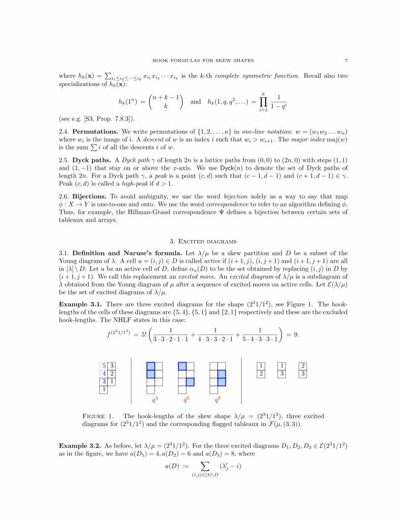
3.1. Definition and Naruse’s formula. Let λ/µ be a skew partition and D be a subset of theYoung diagram of λ. A cell u = (i, j) ∈ D is called active if (i+ 1, j), (i, j+ 1) and (i+ 1, j+ 1) are allin [λ] \D. Let u be an active cell of D, define αu(D) to be the set obtained by replacing (i, j) in D by(i+ 1, j+ 1). We call this replacement an excited move. An excited diagram of λ/µ is a subdiagram ofλ obtained from the Young diagram of µ after a sequence of excited moves on active cells. Let E(λ/µ)be the set of excited diagrams of λ/µ.
Example 3.1. There are three excited diagrams for the shape (231/12), see Figure 1. The hook-lengths of the cells of these diagrams are 5, 4, 5, 1 and 2, 1 respectively and these are the excludedhook-lengths. The NHLF states in this case:
f (231/12) = 5!
(1
3 · 3 · 2 · 1 · 1+
1
4 · 3 · 3 · 2 · 1+
1
5 · 4 · 3 · 3 · 1
)= 9 .
13 1
23
45 1
213
23
q4 q6 q8
Figure 1. The hook-lengths of the skew shape λ/µ = (231/12), three exciteddiagrams for (231/12) and the corresponding flagged tableaux in F(µ, (3, 3)).
Example 3.2. As before, let λ/µ = (231/12). For the three excited diagrams D1, D2, D3 ∈ E(231/12)as in the figure, we have a(D1) = 4, a(D2) = 6 and a(D3) = 8, where
a(D) :=∑
(i,j)∈[λ]\D(λ′j − i)
8 ALEJANDRO MORALES, IGOR PAK, GRETA PANOVA
is the product of powers of q in the numerator of the RHS of (1.4). Now our Theorem 1.4 gives
s(231/12)(1, q, q2, . . .) =
q4
(1− q3)2(1− q2)(1− q)2+
+q6
(1− q4)(1− q3)2(1− q2)(1− q)+
q8
(1− q5)(1− q4)(1− q3)2(1− q).
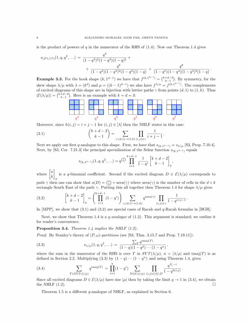
Example 3.3. For the hook shape (k, 1d−1) we have that f (k,1d−1) =(k+d−2k−1
). By symmetry, for the
skew shape λ/µ with λ = (kd) and µ = ((k − 1)d−1) we also have fλ/µ = f (k,1d−1). The complementsof excited diagrams of this shape are in bijection with lattice paths γ from points (d, 1) to (1, k). Thus
|E(λ/µ)| =(k+d−2k−1
). Here is an example with k = d = 3:
q3 q4 q5 q5 q6 q7 .
Moreover, since h(i, j) = i+ j − 1 for (i, j) ∈ [λ] then the NHLF states in this case:
(3.1)
(k + d− 2
k − 1
)=
∑γ:(d,1)→(1,k)
∏(i,j)∈γ
1
i+ j − 1.
Next we apply our first q-analogue to this shape. First, we have that s(k,1d−1) = sλ/µ [S3, Prop. 7.10.4].Next, by [S3, Cor. 7.21.3] the principal specialization of the Schur function s(k,1d−1) equals
s(k,1d−1)(1, q, q2, . . .) = q(
d2)k+d−1∏i=1
1
1− qi
[k + d− 2k − 1
]q
,
where
[nk
]q
is a q-binomial coefficient. Second if the excited diagram D ∈ E(λ/µ) corresponds to
path γ then one can show that a(D) =(n2
)+ area(γ) where area(γ) is the number of cells in the d× k
rectangle South East of the path γ. Putting this all together then Theorem 1.4 for shape λ/µ gives
(3.2)
[k + d− 2k − 1
]q
=
(k+d−1∏i=1
(1− qi)
) ∑γ:(d,1)→(1,k)
qarea(γ)∏
(i,j)∈γ
1
1− qi+j−1.
In [MPP], we show that (3.1) and (3.2) are special cases of Racah and q-Racah formulas in [BGR].
Next, we show that Theorem 1.4 is a q-analogue of (1.2). This argument is standard; we outline itfor reader’s convenience.
Proposition 3.4. Theorem 1.4 implies the NHLF (1.2).
Proof. By Stanley’s theory of (P, ω)-partitions (see [S3, Thm. 3.15.7 and Prop. 7.19.11]):
(3.3) sλ/µ(1, q, q2, . . .) =
∑T q
tmaj(T )
(1− q)(1− q2) · · · (1− qn),
where the sum in the numerator of the RHS is over T in SY T (λ/µ), n = |λ/µ| and tmaj(T ) is asdefined in Section 2.2. Multiplying (3.3) by (1− q) · · · (1− qn) and using Theorem 1.4, gives
(3.4)∑
T∈SYT(λ/µ)
qtmaj(T ) =
n∏i=1
(1− qi)∑
D∈E(λ/µ)
∏(i,j)∈[λ]\D
qλ′j−i
1− qh(i,j).
Since all excited diagrams D ∈ E(λ/µ) have size |µ| then by taking the limit q → 1 in (3.4), we obtainthe NHLF (1.2).
Theorem 1.5 is a different q-analogue of NHLF, as explained in Section 6.
HOOK FORMULAS FOR SKEW SHAPES 9
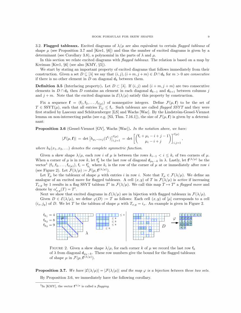
3.2. Flagged tableaux. Excited diagrams of λ/µ are also equivalent to certain flagged tableaux ofshape µ (see Proposition 3.7 and [Kre1, §6]) and thus the number of excited diagrams is given by adeterminant (see Corollary 3.8), a polynomial in the parts of λ and µ.
In this section we relate excited diagrams with flagged tableaux. The relation is based on a map byKreiman [Kre1, §6] (see also [KMY, §5]).
We start by stating an important property of excited diagrams that follows immediately from theirconstruction. Given a set D ⊆ [λ] we say that (i, j), (i+m, j +m) ∈ D ∩ dk for m > 0 are consecutiveif there is no other element in D on diagonal dk between them.
Definition 3.5 (Interlacing property). Let D ⊂ [λ]. If (i, j) and (i + m, j + m) are two consecutiveelements in D ∩ dk then D contains an element in each diagonal dk−1 and dk+1 between columns jand j +m. Note that the excited diagrams in E(λ/µ) satisfy this property by construction.
Fix a sequence f = (f1, f2, . . . , f`(µ)) of nonnegative integers. Define F(µ, f) to be the set ofT ∈ SSYT(µ), such that all entries Tij ≤ fi. Such tableaux are called flagged SSYT and they werefirst studied by Lascoux and Schutzenberger [LS] and Wachs [Wac]. By the Lindstrom-Gessel-Viennotlemma on non-intersecting paths (see e.g. [S3, Thm. 7.16.1]), the size of F(µ, f) is given by a determi-nant:
Proposition 3.6 (Gessel-Viennot [GV], Wachs [Wac]). In the notation above, we have:
|F(µ, f)| = det[hµi−i+j(1
fi)]`(µ)
i,j=1= det
[(fi + µi − i+ j − 1
µi − i+ j
)]`(µ)
i,j=1
,
where hk(x1, x2, . . .) denotes the complete symmetric function.
Given a skew shape λ/µ, each row i of µ is between the rows ki−1 < i ≤ ki of two corners of µ.When a corner of µ is in row k, let f ′k be the last row of diagonal dµk−k in λ. Lastly, let f (λ/µ) be thevector1 (f1, f2, . . . , f`(µ)), fi = f ′ki where ki is the row of the corner of µ at or immediately after row i
(see Figure 2). Let F(λ/µ) := F(µ, f (λ/µ)).Let Tµ be the tableaux of shape µ with entries i in row i. Note that Tµ ∈ F(λ/µ). We define an
analogue of an excited move for flagged tableaux. A cell (x, y) of T in F(λ/µ) is active if increasingTx,y by 1 results in a flag SSYT tableau T ′ in F(λ/µ). We call this map T 7→ T ′ a flagged move anddenote by α′x,y(T ) = T ′.
Next we show that excited diagrams in E(λ/µ) are in bijection with flagged tableaux in F(λ/µ).Given D ∈ E(λ/µ), we define ϕ(D) := T as follows: Each cell (x, y) of [µ] corresponds to a cell
(ix, jy) of D. We let T be the tableau of shape µ with Tx,y = ix. An example is given in Figure 2.
µ
λ
≤ 4
≤ 8
≤ 8
≤ 8
≤ 9
fk1= 4
fk2= 8
fk3= 9 D
ϕ1 1 1 1 2 3 32 2 2 43 4 4 66 6 6 78 9
Figure 2. Given a skew shape λ/µ, for each corner k of µ we record the last row fkof λ from diagonal dµk−k. These row numbers give the bound for the flagged tableaux
of shape µ in F(µ, f (λ/µ)).
Proposition 3.7. We have |E(λ/µ)| = |F(λ/µ)| and the map ϕ is a bijection between these two sets.
By Proposition 3.6, we immediately have the following corollary.
1In [KMY], the vector fλ/µ is called a flagging.
10 ALEJANDRO MORALES, IGOR PAK, GRETA PANOVA
Corollary 3.8.
|E(λ/µ)| = det
[(f(λ/µ)i + µi − i+ j − 1
f(λ/µ)i − 1
)]`(µ)
i,j=1
.
Let K(λ/µ) be the set of T ∈ SSYT(µ) such that all entries t = Ti,j satisfy the inequalities t ≤ `(λ)and Ti,j + c(i, j) ≤ λt.
Proposition 3.9 (Kreiman [Kre1]). We have |E(λ/µ)| = |K(λ/µ)| and the map ϕ is a bijectionbetween these two sets.
Since the correspondences ϕ from Propositions 3.7 and 3.9 are the same then both sets of tableauxare equal.
Corollary 3.10. We have F(λ/µ) = K(λ/µ).
Remark 3.11. To clarify the unusual situation in this section, here we have three equinumerous setsK(λ/µ), F(λ/µ) and E(λ/µ), all of which were previously defined in the literature. The first two are infact the same sets, but defined somewhat differently; essentially, the set of inequalities in the definitionof K(λ/µ) is redundant. Since our goal is to prove Corollary 3.8, we find it easier and more instructiveto use Kreiman’s map ϕ with a new analysis (see below), to prove directly that |E(λ/µ)| = |F(λ/µ)|.An alternative approach would be to prove the equality of sets F(λ/µ) = K(λ/µ) first (Corollary 3.10),which reduces the problem to Kreiman’s result (Proposition 3.9).
Proof of Proposition 3.7. We need to prove that ϕ is a well defined map from E(λ/µ) to F(µ, f (λ/µ)).First, let us show that T = ϕ(D) is a SSYT by induction on the number of excited moves of D. First,note that ϕ([µ]) = Tµ which is SSYT. Next, assume that for D ∈ E(λ/µ), T = ϕ(D) is a SSYT andD′ = α(ix,jy)(D) for some active cell (ix, jy) of D corresponding to (x, y) in [µ]. Then T ′ = ϕ(D′)is obtained from T by adding 1 to entry Tx,y = ix and leaving the rest of entries unchanged. When(x + 1, y) ∈ [µ], since (ix + 1, jy) is not in D then the cell of the diagram corresponding to (x + 1, y)is in a row > ix + 1, therefore T ′x,y = ix + 1 < Tx+1,y = T ′x+1,y. Similarly, if (x, y + 1) ∈ [µ], since(ix, jx+1) is not in D then the cell of the diagram corresponding to (x, y+1) is in a row > ix, thereforeT ′x,y = ix + 1 ≤ Tx,y+1 = T ′x,y+1. Thus, T ′ ∈ SSYT(λ/µ).
Next, let us show that T is a flagged tableau in F(µ, f (λ/µ)). Given an excited diagram D, if cell(ix, jy) of D is the cell corresponding to (x, y) in [µ] then the row ix is at most fkx : the last row ofdiagonal dµkx−kx where kx is the row of the corner of µ on or immediately after row x. Thus Tx,y ≤ fkx ,which proves the claim.
Finally, we prove that ϕ is a bijection by building its inverse. Given T ∈ F(µ, f (λ/µ)), let D = ϑ(T )be the set D = (Tx,y, y + Tx,y) | (x, y) ∈ [µ]. Let us show ϑ is a well defined map from F(µ, f (λ/µ))
to E(λ/µ). By definition of the flags f (λ/µ), observe that D is a subset of [λ]. We prove that D is inE(λ/µ) by induction on the number of flagged moves α′x,y(·). First, observe that ϑ(Tµ) = [µ] whichis in E(λ/µ). Assume that for T ∈ F(λ/µ), D = ϑ(T ) is in E(λ/µ) and T ′ = α′x,y(T ) for some activecell (x, y) of T . Note that replacing Tx,y by Tx,y + 1 results in a flagged tableaux T ′ in F(λ/µ) isequivalent to (ix, iy) being an active cell of D. Since ϑ(T ′) = αix,iy (D) and the latter is an excited
diagram, the result follows. By construction, we conclude that ϑ = ϕ−1, as desired.
4. Algebraic proof of Theorem 1.4
4.1. Preliminary results. A skew shape λ/µ with µ ⊆ λ ⊆ d× (n− d) is in correspondence with apair of Grassmannian permutations w v of n both with descent at position d and where is thestrong Bruhat order. Recall that a permutation v = v1v2 · · · vn is Grassmannian if it has a uniquedescent. The permutation v is obtained from the diagram λ by writing the numbers 1, . . . , n along theunit segments of the boundary of λ starting at the bottom left corner and ending at the top right ofthe enclosing d× (n− d) rectangle. The permutation v is obtained by first reading the d numbers on
HOOK FORMULAS FOR SKEW SHAPES 11
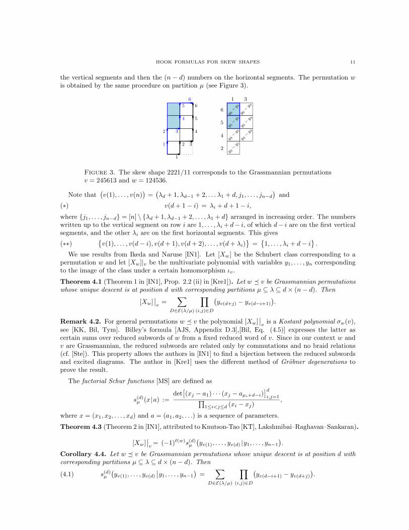
the vertical segments and then the (n − d) numbers on the horizontal segments. The permutation wis obtained by the same procedure on partition µ (see Figure 3).
1
2 3
4
5
6
1
2 3
4
5
6 1 3
6
5
4
2
y 6− y 1
y 6− y 3
y 5− y 1
y 5− y 3
y 4− y 1
y 4− y 3
y 2− y 1
Figure 3. The skew shape 2221/11 corresponds to the Grassmannian permutationsv = 245613 and w = 124536.
Note that(v(1), . . . , v(n)
)=(λd + 1, λd−1 + 2, . . . λ1 + d, j1, . . . , jn−d
)and
v(d+ 1− i) = λi + d+ 1− i,(∗)where j1, . . . , jn−d = [n] \ λd + 1, λd−1 + 2, . . . , λ1 + d arranged in increasing order. The numberswritten up to the vertical segment on row i are 1, . . . , λi + d− i, of which d− i are on the first verticalsegments, and the other λi are on the first horizontal segments. This gives
(∗∗)v(1), . . . , v(d− i), v(d+ 1), v(d+ 2), . . . , v(d+ λi)
=
1, . . . , λi + d− i.
We use results from Ikeda and Naruse [IN1]. Let [Xw] be the Schubert class corresponding to apermutation w and let [Xw]|v be the multivariate polynomial with variables y1, . . . , yn correspondingto the image of the class under a certain homomorphism ιv.
Theorem 4.1 (Theorem 1 in [IN1], Prop. 2.2 (ii) in [Kre1]). Let w v be Grassmannian permutationswhose unique descent is at position d with corresponding partitions µ ⊆ λ ⊆ d× (n− d). Then
[Xw]∣∣v
=∑
D∈E(λ/µ)
∏(i,j)∈D
(yv(d+j) − yv(d−i+1)
).
Remark 4.2. For general permutations w v the polynomial [Xw]∣∣v
is a Kostant polynomial σw(v),
see [KK, Bil, Tym]. Billey’s formula [AJS, Appendix D.3],[Bil, Eq. (4.5)] expresses the latter ascertain sums over reduced subwords of w from a fixed reduced word of v. Since in our context w andv are Grassmannian, the reduced subwords are related only by commutations and no braid relations(cf. [Ste]). This property allows the authors in [IN1] to find a bijection between the reduced subwordsand excited diagrams. The author in [Kre1] uses the different method of Grobner degenerations toprove the result.
The factorial Schur functions [MS] are defined as
s(d)µ (x |a) :=
det[(xj − a1) · · · (xj − aµi+d−i)
]di,j=1∏
1≤i<j≤d (xi − xj),
where x = (x1, x2, . . . , xd) and a = (a1, a2, . . .) is a sequence of parameters.
Theorem 4.3 (Theorem 2 in [IN1], attributed to Knutson-Tao [KT], Lakshmibai–Raghavan–Sankaran).
[Xw]∣∣v
= (−1)`(w)s(d)µ
(yv(1), . . . , yv(d) |y1, . . . , yn−1
).
Corollary 4.4. Let w v be Grassmannian permutations whose unique descent is at position d withcorresponding partitions µ ⊆ λ ⊆ d× (n− d). Then
(4.1) s(d)µ
(yv(1), . . . , yv(d)
∣∣y1, . . . , yn−1
)=
∑D∈E(λ/µ)
∏(i,j)∈D
(yv(d−i+1) − yv(d+j)
).
12 ALEJANDRO MORALES, IGOR PAK, GRETA PANOVA
Proof. Combining Theorem 4.1 and Theorem 4.3 we get
(−1)`(w)s(d)µ (yv(1), . . . , yv(d)
∣∣y1, . . . , yn−1) =∑
D∈E(λ/µ)
∏(i,j)∈D
(yv(d+j) − yv(d−i+1)
).(4.2)
Note that `(w) = |µ| and `(v) = |λ|, so we can remove the (−1)`(w) on the left of (4.2) by negating alllinear terms on the right and get the desired result.
4.2. Proof of Theorem 1.4. First we use Corollary 4.4 to get an identity of rational functions iny = (y1, y2, . . . , yn) (Lemma 4.5). Then we evaluate this identity at yp = qp−1 and use some identitiesof symmetric functions to prove the theorem. Let
Hi,r(y) :=
λi+d−i∏
p=µr+d+1−r
(yλi+d+1−i − yp
)−1if µr + d− r ≤ λi + d− i,
0 otherwise.
.
Lemma 4.5.
(4.3) det[Hi,j(y)
]di,r=1
=∑
D∈E(λ/µ)
∏(i,j)∈[λ]\D
1
yv(d+1−i) − yv(d+j).
Proof. Start with (4.1) and divide both sides by
(4.4)∏
(i,j)∈[λ]
(yv(d+1−i) − yv(d+j)
)=
d∏i=1
λi∏j=1
(yv(d+1−i) − yv(d+j)
),
to obtain
(4.5)s
(d)µ (yv(1), . . . , yv(d)|y1, . . . , yn−1)∏
(i,j)∈[λ](yv(d+1−i) − yv(d+j))=
∑D∈E(λ/µ)
∏(i,j)∈[λ]\D
1
yv(d+1−i) − yv(d+j).
Denote the LHS of (4.5) by Sλ,µ(y). By the determinantal formula for factorial Schur functionsand by (4.4) we have
Sλ,µ(y) =det[∏µr+d−r
p=1 (yv(d+1−i) − yp)]di,r=1∏d
i=1
∏dk=i+1(yv(d+1−i) − yv(d+1−k))
· 1∏di=1
∏λij=1(yv(d+1−i) − yv(d+j))
= det
[ ∏µr+d−rp=1 (yv(d+1−i) − yp)∏d
k=i+1(yv(d+1−i) − yv(d+1−k))∏λij=1(yv(d+1−i) − yv(d+j))
]di,r=1
.
Using (∗∗) in the denominator of the matrix entry, we obtain:
Sλ,µ(y) = det
[µr+d−r∏p=1
(yv(d+1−i) − yp)λi+d−i∏p=1
(yv(d+1−i) − yp)−1
]di,r=1
.(4.6)
By (∗), we have v(d+1− i) = λi+d+1− i. Therefore, the matrix entry on the RHS of (4.6) simplifiesto Hi,r(y).
(4.7) Sλ,µ(y) = det[Hi,r(y)]di,r=1 .
Combining (4.7) with (4.5) we obtain (4.3) as desired.
HOOK FORMULAS FOR SKEW SHAPES 13
Next, we evaluate yp = qp−1 for p = 1, . . . , n in (4.3). Since
(4.8) (yv(d+1−i) − yv(d+j))∣∣∣yp=qp
= qλi+d+1−i − qd−λ′j+j = −qd−λ
′j+j(1− qh(i,j)) ,
we obtain
(4.9) det[Hi,r(1, q, q
2, . . . , qn−1)]di,r=1
= (−1)|λ|−|µ|∑
D∈E(λ/µ)
∏(i,j)∈[λ]\D
q−d+λ′j−j
1− qh(i,j).
We now simplify the matrix entry Hi,r(1, q, q2, . . . , qn−1). For ν = (ν1, . . . , νd), let
g(ν) :=
d∑i=1
(νi + d+ 1− i
2
).
We then have:
Proposition 4.6.
Hi,r(1, q, q2, . . . , qn−1) = q−g(λ)+g(µ)hλi−i−µr+r(1, q, q
2, . . .) ,
where hk(x) denotes the k-th complete symmetric function.
Proof. We have:
Hi,r(1, q, q2, . . . , qn−1) =
λi+d−i∏p=µr+d+1−r
1
qλi+d+1−i − qp
= (−1)λi−i−µr+r q−g(λ)+g(µ)
λi−i−µr+r∏p=1
1
1− qp
= (−1)λi−i−µr+r q−g(λ)+g(µ) hλi−i−µr+r(1, q, q2, . . .) ,
where the last identity follows by the principal specialization of the complete symmetric function.
Using Proposition 4.6, the LHS of (4.9) becomes
(4.10)det[Hi,r(1, q, . . . , q
n−1)]di,r=1
= (−1)|λ|−|µ|q−g(λ)+g(µ) det[hλi−i−µr+r(1, q, q
2, . . .)]di,r=1
= (−1)|λ|−|µ|q−g(λ)+g(µ)sλ/µ(1, q, q2, . . .) ,
where the last equality follows by the Jacobi-Trudi identity for skew Schur functions (2.1). From here,rearranging powers of q and cancelling signs, equation (4.9) becomes
(4.11) sλ/µ(1, q, q2, . . .) = qg(λ)−g(µ)∑
D∈E(λ/µ)
∏(i,j)∈[λ]\D
q−d+λ′j−j
1− qh(i,j).
It remains to match the powers of q in (4.11) and (1.4).
Proposition 4.7. For an excited diagram D ∈ E(λ/µ) we have:
g(λ)− g(µ) +∑
(i,j)∈[λ]\D(−d+ λ′j − j) =
∑(i,j)∈[λ]\D
(λ′j − i) .
Proof. Note that g(λ) = d|λ|+∑
(i,j)∈[λ] c(i, j), where c(i, j) = j − i. Therefore,
g(λ)− g(µ)−∑
(i,j)∈[λ]\Dd = g(λ)− g(µ)− d(|λ| − |D|) =
∑(i,j)∈[λ]
c(i, j)−∑
(i,j)∈[µ]
c(i, j) .
14 ALEJANDRO MORALES, IGOR PAK, GRETA PANOVA
Finally, notice that the cells of any excited diagram D have the same multiset of content values, sinceevery excited move is along a diagonal and the content of the moved cell j− i remains constant. Thusthe power of q for each term becomes∑
(i,j)∈[λ]\[µ]
c(i, j) +∑
(i,j)∈[λ]\D(λ′j − j) =
∑(i,j)∈[λ]\D
(c(i, j) + λ′j − j
)=
∑(i,j)∈[λ]\D
λ′j − i ,
as desired.
Using Proposition 4.7 on the RHS of (4.11) yields (1.4) finishing the proof of Theorem 1.4.
5. The Hillman-Grassl and the RSK correspondences
5.1. The Hillman-Grassl correspondence. Recall the Hillman-Grassl correspondence which de-fines a map between RPP π of shape λ and arrays A of nonnegative integers of shape λ such that|π| =
∑u∈[λ]Auh(u). Let A(λ) be the set of such arrays. The weight ω(A) of A is the sum
ω(A) :=∑u∈λAuh(u). We review this construction and some of its properties (see [S3, §7.22]
and [Sag2, §4.2]). We denote by Φ the Hillman-Grassl map Φ : π 7→ A.
Definition 5.1 (Hillman-Grassl map Φ). Given a reverse plane partition π of shape λ, let A be anarray of zeroes of shape λ. Next we find a path p of North and East steps in π as follows:
(i) Start p with the most South-Western nonzero entry in π. Let cs be the column of such anentry.
(ii) If p has reached (i, j) and πi,j = πi−1,j > 0 then p moves North to (i − 1, j), otherwise if0 < πi,j < πi−1,j then p moves East to (i+ 1, j).
(iii) The path p terminates when the previous move is not possible in a cell at row rf .Let π′ be obtained from π by subtracting 1 from every entry in p. Note that π′ is still a RPP. In thearray A we add 1 in position Acs,rf and obtain array A′. We iterate these three steps until we reacha plane partition of zeroes. We map π to the final array A.
Theorem 5.2 ([HiG]). The map Φ : RPP(λ)→ A(λ) is a bijection.
Note that if A = Φ(π) then |π| = ω(A) so as a corollary we obtain (1.6). Let us now describe theinverse Ω : A 7→ π of the Hillman-Grassl map.
Definition 5.3 (Inverse Hillman-Grassl map Φ−1). Given an array A of nonnegative integers ofshape λ, let π be the RPP of shape λ of all zeroes. Next, we order the nonzero entries of A, countingmultiplicities, with the order (i, j) < (i′, j′) if j > j′ or j = j′ and i < i′ (i.e. (i, j) is right of (i′, j′)or higher in the same column). Next, for each entry (rs, cj) of A in this order (i1, j1), . . . , (im, jm) webuild a reverse path q of South and West steps in π starting at row rs and ending in column cf asfollows:
(i) Start q with the most Eastern entry of π in row rs.(ii) If q has reached (i, j) and πi,j = πi+1,j then q moves South to (i − 1, j), otherwise q moves
West to (i+ 1, j).(iii) Path q ends when it reaches the Southern entry of π in column cf .
Step (iii) is actually attained (see e.g. [Sag2, Lemma 4.2.4]. Let π′ be obtained from π by adding 1from every entry in q. Note that π′ is still a RPP. In the array A we subtract 1 in position Acf ,rs andobtain array A′. We iterate this process following the order of the nonzero entries of A until we reachan array of zeroes. We map A to the final RPP π. Note that ω(A) = |π|.
Theorem 5.4 ([HiG]). We have Ω = Φ−1.
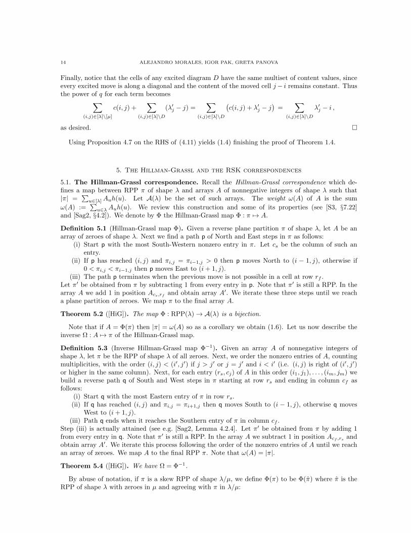
By abuse of notation, if π is a skew RPP of shape λ/µ, we define Φ(π) to be Φ(π) where π is theRPP of shape λ with zeroes in µ and agreeing with π in λ/µ:
HOOK FORMULAS FOR SKEW SHAPES 15
0120
1
0110
1
012 0
0101
11
0121
2
012
00 0
00001
11
0122
3
01Φ Φ Φ
Recall that unlike for straight shapes, the enumeration of SSYT and RPP of skew shape are notequivalent. Therefore, the image Φ(SSYT(λ/µ)) is a strict subset of Φ(RPP(λ/µ)). In Section 7 wecharacterize the SSYT case in terms of excited diagrams, and in Section 6 we characterize the RPPcase in terms of new diagrams called pleasant diagrams. Both characterizations require a few propertiesof Φ that we review next.
5.2. The Hillman-Grassl correspondence and Greene’s theorem. In this section we review keyproperties of the Hillman-Grassl correspondence related to the RSK correspondence [S3, §7.11]. Wedenote Ψ : M 7→ (P,Q), where M is a matrix with nonnegative integer entries and I(Ψ(M)) := P ,R(Ψ(M)) := Q are SSYT of the same shape called the insertion and recording tableau, respectively.
Given a reverse plane partition π and an integer k with 1− `(λ) ≤ k ≤ λ1 − 1, a k-diagonal is thesequence of entries (πij) with i − j = k. Each k-diagonal of π is nonincreasing and so we denote it
by a partition ν(k). The k-trace of π denoted by trk(π) is the sum of the parts of ν(k). Note that the0-trace of π is the standard trace tr(π) =
∑i πi,i.
Given the Young diagram of λ and an integer k with 1 − `(λ) ≤ k ≤ λ1 − 1, let λk be the largesti × (i + k) rectangle that fits inside the Young diagram starting at (1, 1). For k = 0, the rectangleλ0 = λ is the (usual) Durfee square of λ. Given an array A of shape λ, let Ak be the subarray of Aconsisting of the cells inside λk and |Ak| be the sum of its entries. Also, given a rectangular array B,
let Bl and B↔ denote the arrays B flipped vertically and horizontally, respectively. Here vertical flipmeans that the bottom row become the top row, and horizontal means that the rightmost columnbecomes the leftmost column.
In the construction Φ−1, entry 1 in position (i, j) adds 1 to the k-trace if and only if (i, j) ∈ λk .This observation implies the following result.
Proposition 5.5 (Gansner, Thm. 3.2 in [G1]). Let A = Φ(π) then for k with 1− `(λ) ≤ k ≤ λ1 − 1we have
trk(π) = |Ak|.
As a corollary, when k = 0, Proposition 5.5 gives Gansner’s formula (1.7) for the generating seriesfor RPP(λ) by size and trace. Indeed, the generating function for the arrays is a product over cells(i, j) ∈ [λ] of terms which contain t in the numerator if only if (i, j) ∈ λ. We refer to [G1] for thedetails.
Let us note that not only is the k-trace determined by Proposition 5.5 but also the parts of ν(k).This next result states that the partition ν(k) and its conjugate are determined by nondecreasing andnonincreasing chains in the rectangle Ak.
Given an m × n array M = (mij) of nonnegative integers, an ascending chain of length s of Mis a sequence c := ((i1, j1), (i2, j2), . . . , (is, js)) where m ≥ i1 ≥ · · · ≥ is ≥ 1 and 1 ≤ j1 ≤ · · · ≤js ≤ n where (i, j) appears in c at most mij times. A descending chain of length s is a sequenced := ((i1, j1), (i2, j2), . . . , (is, js)) where 1 ≤ i1 < · · · < is ≤ m and 1 ≤ j1 < · · · < js ≤ n where (i, j)appears in d only if mij 6= 0.
Let ac1(M) and dc1(M) be the length of the longest ascending and descending chains in M respec-tively. In general for t ≥ 1, let act(M) be the maximum combined length of t ascending chains wherethe combined number of times (i, j) appears is mij . We define dct(M) analogously for descendingchains.
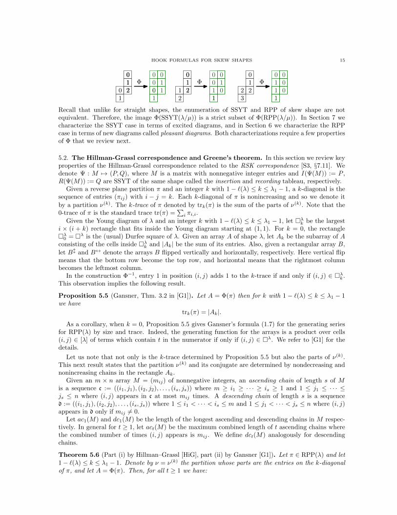
Theorem 5.6 (Part (i) by Hillman–Grassl [HiG], part (ii) by Gansner [G1]). Let π ∈ RPP(λ) and let1− `(λ) ≤ k ≤ λ1 − 1. Denote by ν = ν(k) the partition whose parts are the entries on the k-diagonalof π, and let A = Φ(π). Then, for all t ≥ 1 we have:
16 ALEJANDRO MORALES, IGOR PAK, GRETA PANOVA
(i) act(Ak) = ν1 + ν2 + · · ·+ νt,(ii) dct(Ak) = ν′1 + ν′2 + · · ·+ ν′t.
Remark 5.7. This result is the analogue of Greene’s theorem for the RSK correspondence Ψ, seee.g. [S3, Thm. A.1.1.1]. In fact, we have the following explicit connection with RSK.
Corollary 5.8. Let π be in RPP(λ), A = Φ(π), and let k be an integer 1− `(λ) ≤ k ≤ λ1−1. Denote
by ν(k) is the partition obtained from the k-diagonal of π. Then the shape of the tableaux in Ψ(Akl)
and Ψ(Ak↔) is equal to ν(k).
Example 5.9. Let λ = (4, 4, 3, 1) and π ∈ RPP(λ) be as below. Then we have:
π = 0 1 3 41 3 5 63 6 73
A = Φ(π) = 0 2 1 11 1 1 22 1 10
Note that ν(0) = (7, 3) and indeed `(ν(0)) = 2 = dc1(A0). For example, take d = (2, 2), (3, 3).Similarly, ν(1) = (5, 1), `(ν(1)) = 2 = dc1(A1). Applying the RSK to A1
↔ and A0↔ we get tableaux
of shape ν(1) and ν(0), respectively:
I(Ψ(A1↔)) = I(Ψ 1 2 0
1 1 1) = 1 1 2 2 3
2, I(Ψ(A0
↔)) = I(Ψ 1 2 01 1 11 1 2
) = 1 1 1 2 2 3 32 2 3
.
6. Hillman-Grassl map on skew RPP
In this section we show that the Hillman-Grassl map is a bijection between RPP of skew shape andarrays of nonnegative integers with support on certain diagrams related to excited diagrams.
6.1. Pleasant diagrams. We identify any diagram S (set of boxes in [λ]) with its corresponding 0-1indicator array, i.e. array of shape λ and support S.
Definition 6.1 (Pleasant diagrams). A diagram S ⊂ [λ] is a pleasant diagram of λ/µ if for all integersk with 1 − `(λ) ≤ k ≤ λ1 − 1, the subarray Sk := S ∩ λk has no descending chain bigger than thelength sk of the diagonal dk of λ/µ, i.e. for every k we have dc1(Sk) ≤ sk. We denote the set ofpleasant diagrams of λ/µ by P(λ/µ).
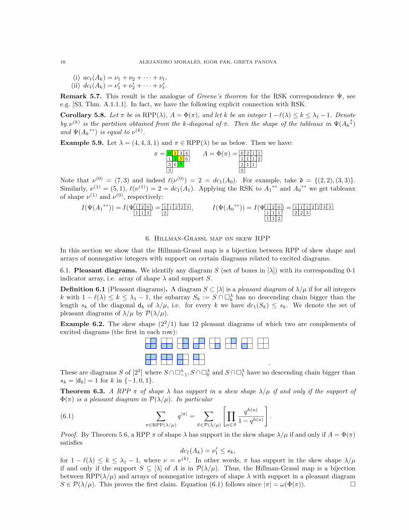
Example 6.2. The skew shape (22/1) has 12 pleasant diagrams of which two are complements ofexcited diagrams (the first in each row):
.
These are diagrams S of [22] where S ∩λ−1, S ∩λ0 and S ∩λ1 have no descending chain bigger thansk = |dk| = 1 for k in −1, 0, 1.Theorem 6.3. A RPP π of shape λ has support in a skew shape λ/µ if and only if the support ofΦ(π) is a pleasant diagram in P(λ/µ). In particular
(6.1)∑
π∈RPP(λ/µ)
q|π| =∑
S∈P(λ/µ)
[∏u∈S
qh(u)
1− qh(u)
].
Proof. By Theorem 5.6, a RPP π of shape λ has support in the skew shape λ/µ if and only if A = Φ(π)satisfies
dc1(Ak) = ν′1 ≤ sk,for 1 − `(λ) ≤ k ≤ λ1 − 1, where ν = ν(k). In other words, π has support in the skew shape λ/µif and only if the support S ⊆ [λ] of A is in P(λ/µ). Thus, the Hillman-Grassl map is a bijectionbetween RPP(λ/µ) and arrays of nonnegative integers of shape λ with support in a pleasant diagramS ∈ P(λ/µ). This proves the first claim. Equation (6.1) follows since |π| = ω(Φ(π)).
HOOK FORMULAS FOR SKEW SHAPES 17
Remark 6.4. Theorem 1.5 gives an alternative description for pleasant diagrams P(λ/µ) as thesupports of 0-1 arrays A of shape λ such that Φ−1(A) is in RPP(λ/µ).
We also give a generalization of the trace generating function (1.7) for these reverse plane partitions.
Proof of Theorem 1.7. Given a pleasant diagram S ∈ P(λ/µ), let BS be the collection of arrays ofshape λ with support in S. Given a RPP π, let A = Φ(π). By Theorem 6.3 π has shape λ/µ if andonly if A has support in a pleasant diagram S in P(λ/µ). Thus
(6.2)∑
π∈RPP(λ/µ)
q|π| ttr(π) =∑
S∈P(λ/µ)
∑π∈Φ−1(BS)
q|π| ttr(π) ,
where for each S ∈ P(λ/µ) we have
(6.3)∑
π∈Φ−1(BS)
q|π| =∏u∈S
qh(u)
1− qh(u).
Next, by Proposition 5.5 for k = 0, the trace tr(π) equals |A0|, the sum of the entries of A in theDurfee square λ of λ. Therefore, we refine (6.3) to keep track of the trace of the RPP and obtain
(6.4)∑
π∈Φ−1(BS)
q|π| ttr(π) =∏
u∈S∩λ
tqh(u)
1− tqh(u)
∏u∈S\λ
qh(u)
1− qh(u).
Combining (6.2) and (6.4) gives the desired result.
6.2. Combinatorial proof of NHLF (1.2): relation between pleasant and excited diagrams.Theorem 1.4 relates SSYT of skew shape with excited diagrams and Theorem 6.3 relates RPP of skewshape with pleasant diagrams. Since SSYT are RPP then we expect a relation between pleasant andexcited diagrams of a fixed skew shape λ/µ. The first main result of this subsection characterizes thepleasant diagrams of maximal size in terms of excited diagrams. The second main result of the nextsubsection characterizes all pleasant diagrams.
The key towards these results is a more graphical characterization of pleasant diagrams as describedin the proof of Lemma 6.6. It makes the relationship with excited diagrams more apparent and alsoallows for a more intuitive description for both kinds of diagrams.
Theorem 6.5. A pleasant diagram S ∈ P(λ/µ) has size |S| ≤ |λ/µ| and has maximal size |S| = |λ/µ|if and only if the complement [λ] \ S is an excited diagram in E(λ/µ).
By combining this theorem with Theorem 6.3 we derive again the NHLF. In contrast with thederivation of this formula in Proposition 3.4, this derivation is entirely combinatorial.
First proof of the NHLF (1.2). By Stanley’s theory of P -partitions, [S3, Thm. 3.15.7]
(6.5)∑
π∈RPP(λ/µ)
q|π| =
∑w∈L(Pλ/µ) q
maj(w)∏ni=1(1− qi)
,
where n = |λ/µ| and the sum in the numerator of the RHS is over linear extensions w of the posetPλ/µ with a natural labelling. Multiplying (6.5) by (1− q) · · · (1− qn), and using Theorem 1.5 gives
(6.6)∑
w∈L(Pλ/µ)
qmaj(w) =
n∏i=1
(1− qi)∑
S∈P(λ/µ)
∏u∈S
qh(u)
1− qh(u).
By Theorem 6.5, pleasant diagrams S ∈ P(λ/µ) have size |S| ≤ n, with the equality here exactlywhen S ∈ E(λ/µ). Thus, letting q → 1 in (6.6) gives fλ/µ on the LHS. On RHS, we obtain the sumof products ∏
u∈S
1
h(u),
18 ALEJANDRO MORALES, IGOR PAK, GRETA PANOVA
over all excited diagrams S ∈ E(λ/µ). This implies the NHLF (1.2).
Lemma 6.6. Let S ∈ P(λ/µ). Then there is an excited diagram D ∈ E(λ/µ), such that S ⊆ [λ] \D.
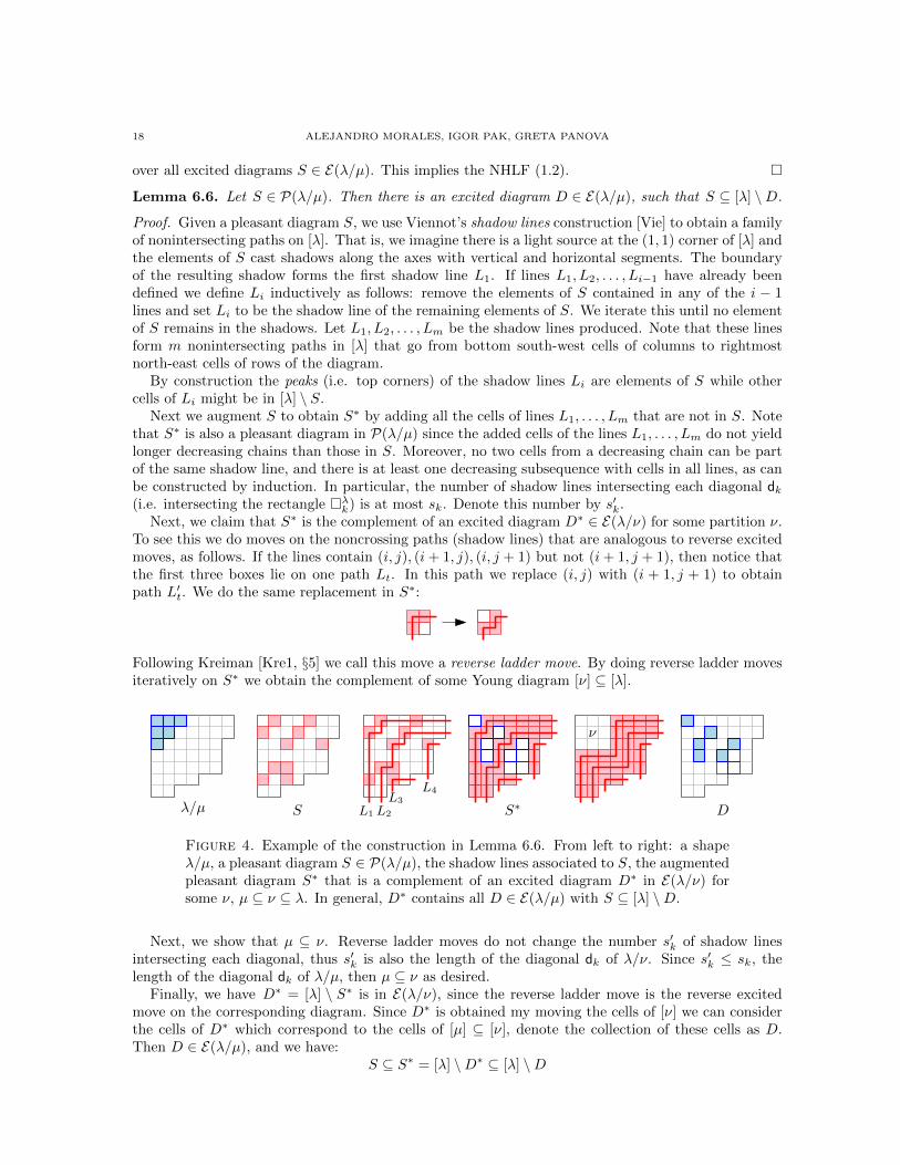
Proof. Given a pleasant diagram S, we use Viennot’s shadow lines construction [Vie] to obtain a familyof nonintersecting paths on [λ]. That is, we imagine there is a light source at the (1, 1) corner of [λ] andthe elements of S cast shadows along the axes with vertical and horizontal segments. The boundaryof the resulting shadow forms the first shadow line L1. If lines L1, L2, . . . , Li−1 have already beendefined we define Li inductively as follows: remove the elements of S contained in any of the i − 1lines and set Li to be the shadow line of the remaining elements of S. We iterate this until no elementof S remains in the shadows. Let L1, L2, . . . , Lm be the shadow lines produced. Note that these linesform m nonintersecting paths in [λ] that go from bottom south-west cells of columns to rightmostnorth-east cells of rows of the diagram.
By construction the peaks (i.e. top corners) of the shadow lines Li are elements of S while othercells of Li might be in [λ] \ S.
Next we augment S to obtain S∗ by adding all the cells of lines L1, . . . , Lm that are not in S. Notethat S∗ is also a pleasant diagram in P(λ/µ) since the added cells of the lines L1, . . . , Lm do not yieldlonger decreasing chains than those in S. Moreover, no two cells from a decreasing chain can be partof the same shadow line, and there is at least one decreasing subsequence with cells in all lines, as canbe constructed by induction. In particular, the number of shadow lines intersecting each diagonal dk(i.e. intersecting the rectangle λk) is at most sk. Denote this number by s′k.
Next, we claim that S∗ is the complement of an excited diagram D∗ ∈ E(λ/ν) for some partition ν.To see this we do moves on the noncrossing paths (shadow lines) that are analogous to reverse excitedmoves, as follows. If the lines contain (i, j), (i+ 1, j), (i, j + 1) but not (i+ 1, j + 1), then notice thatthe first three boxes lie on one path Lt. In this path we replace (i, j) with (i + 1, j + 1) to obtainpath L′t. We do the same replacement in S∗:
Following Kreiman [Kre1, §5] we call this move a reverse ladder move. By doing reverse ladder movesiteratively on S∗ we obtain the complement of some Young diagram [ν] ⊆ [λ].
S L1 L2
L3
L4
S∗
ν
λ/µ D
Figure 4. Example of the construction in Lemma 6.6. From left to right: a shapeλ/µ, a pleasant diagram S ∈ P(λ/µ), the shadow lines associated to S, the augmentedpleasant diagram S∗ that is a complement of an excited diagram D∗ in E(λ/ν) forsome ν, µ ⊆ ν ⊆ λ. In general, D∗ contains all D ∈ E(λ/µ) with S ⊆ [λ] \D.
Next, we show that µ ⊆ ν. Reverse ladder moves do not change the number s′k of shadow linesintersecting each diagonal, thus s′k is also the length of the diagonal dk of λ/ν. Since s′k ≤ sk, thelength of the diagonal dk of λ/µ, then µ ⊆ ν as desired.
Finally, we have D∗ = [λ] \ S∗ is in E(λ/ν), since the reverse ladder move is the reverse excitedmove on the corresponding diagram. Since D∗ is obtained my moving the cells of [ν] we can considerthe cells of D∗ which correspond to the cells of [µ] ⊆ [ν], denote the collection of these cells as D.Then D ∈ E(λ/µ), and we have:
S ⊆ S∗ = [λ] \D∗ ⊆ [λ] \D
HOOK FORMULAS FOR SKEW SHAPES 19
and the statement follows.
We prove Theorem 6.5 via three lemmas.
Lemma 6.7. For all D ∈ E(λ/µ), we have [λ] \D ∈ P(λ/µ).
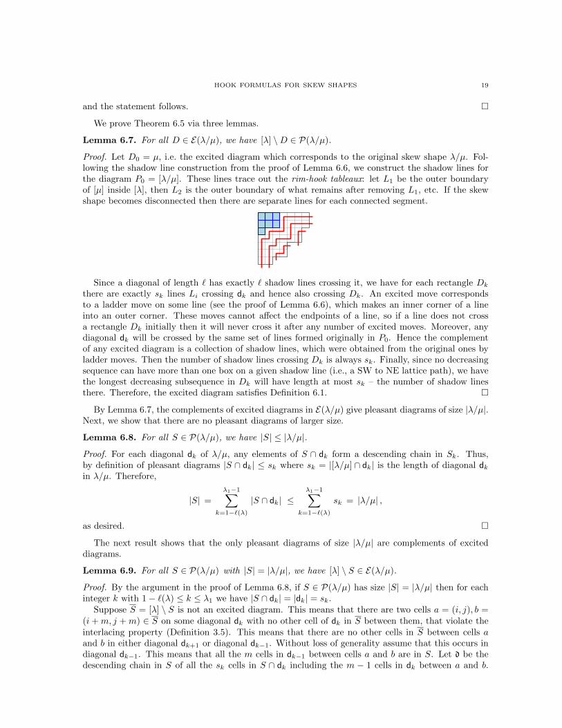
Proof. Let D0 = µ, i.e. the excited diagram which corresponds to the original skew shape λ/µ. Fol-lowing the shadow line construction from the proof of Lemma 6.6, we construct the shadow lines forthe diagram P0 = [λ/µ]. These lines trace out the rim-hook tableaux: let L1 be the outer boundaryof [µ] inside [λ], then L2 is the outer boundary of what remains after removing L1, etc. If the skewshape becomes disconnected then there are separate lines for each connected segment.
Since a diagonal of length ` has exactly ` shadow lines crossing it, we have for each rectangle Dk
there are exactly sk lines Li crossing dk and hence also crossing Dk. An excited move correspondsto a ladder move on some line (see the proof of Lemma 6.6), which makes an inner corner of a lineinto an outer corner. These moves cannot affect the endpoints of a line, so if a line does not crossa rectangle Dk initially then it will never cross it after any number of excited moves. Moreover, anydiagonal dk will be crossed by the same set of lines formed originally in P0. Hence the complementof any excited diagram is a collection of shadow lines, which were obtained from the original ones byladder moves. Then the number of shadow lines crossing Dk is always sk. Finally, since no decreasingsequence can have more than one box on a given shadow line (i.e., a SW to NE lattice path), we havethe longest decreasing subsequence in Dk will have length at most sk – the number of shadow linesthere. Therefore, the excited diagram satisfies Definition 6.1.
By Lemma 6.7, the complements of excited diagrams in E(λ/µ) give pleasant diagrams of size |λ/µ|.Next, we show that there are no pleasant diagrams of larger size.
Lemma 6.8. For all S ∈ P(λ/µ), we have |S| ≤ |λ/µ|.
Proof. For each diagonal dk of λ/µ, any elements of S ∩ dk form a descending chain in Sk. Thus,by definition of pleasant diagrams |S ∩ dk| ≤ sk where sk = |[λ/µ] ∩ dk| is the length of diagonal dkin λ/µ. Therefore,
|S| =
λ1−1∑k=1−`(λ)
|S ∩ dk| ≤λ1−1∑
k=1−`(λ)
sk = |λ/µ| ,
as desired.
The next result shows that the only pleasant diagrams of size |λ/µ| are complements of exciteddiagrams.
Lemma 6.9. For all S ∈ P(λ/µ) with |S| = |λ/µ|, we have [λ] \ S ∈ E(λ/µ).
Proof. By the argument in the proof of Lemma 6.8, if S ∈ P(λ/µ) has size |S| = |λ/µ| then for eachinteger k with 1− `(λ) ≤ k ≤ λ1 we have |S ∩ dk| = |dk| = sk.
Suppose S = [λ] \ S is not an excited diagram. This means that there are two cells a = (i, j), b =(i + m, j + m) ∈ S on some diagonal dk with no other cell of dk in S between them, that violate theinterlacing property (Definition 3.5). This means that there are no other cells in S between cells aand b in either diagonal dk+1 or diagonal dk−1. Without loss of generality assume that this occurs indiagonal dk−1. This means that all the m cells in dk−1 between cells a and b are in S. Let d be thedescending chain in S of all the sk cells in S ∩ dk including the m − 1 cells in dk between a and b.
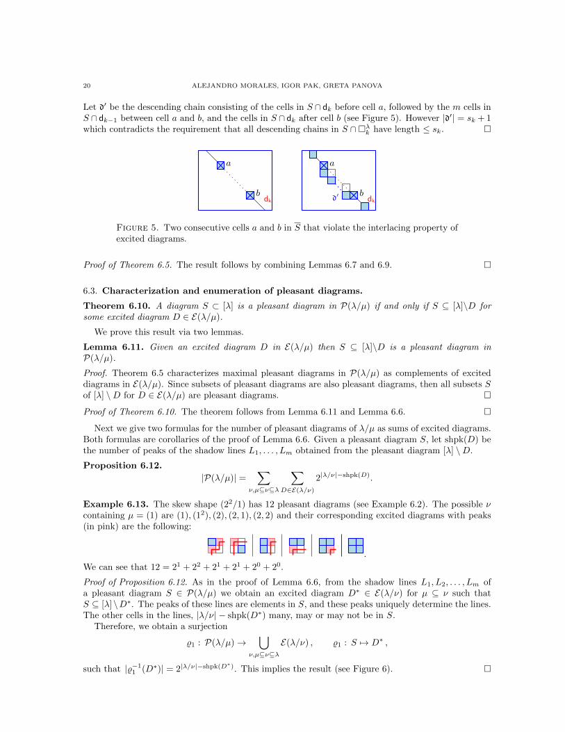
20 ALEJANDRO MORALES, IGOR PAK, GRETA PANOVA
Let d′ be the descending chain consisting of the cells in S ∩ dk before cell a, followed by the m cells inS ∩ dk−1 between cell a and b, and the cells in S ∩ dk after cell b (see Figure 5). However |d′| = sk + 1which contradicts the requirement that all descending chains in S ∩λk have length ≤ sk.
a
b
a
bd′ dkdk
Figure 5. Two consecutive cells a and b in S that violate the interlacing property ofexcited diagrams.
Proof of Theorem 6.5. The result follows by combining Lemmas 6.7 and 6.9.
6.3. Characterization and enumeration of pleasant diagrams.
Theorem 6.10. A diagram S ⊂ [λ] is a pleasant diagram in P(λ/µ) if and only if S ⊆ [λ]\D forsome excited diagram D ∈ E(λ/µ).
We prove this result via two lemmas.
Lemma 6.11. Given an excited diagram D in E(λ/µ) then S ⊆ [λ]\D is a pleasant diagram inP(λ/µ).
Proof. Theorem 6.5 characterizes maximal pleasant diagrams in P(λ/µ) as complements of exciteddiagrams in E(λ/µ). Since subsets of pleasant diagrams are also pleasant diagrams, then all subsets Sof [λ] \D for D ∈ E(λ/µ) are pleasant diagrams.
Proof of Theorem 6.10. The theorem follows from Lemma 6.11 and Lemma 6.6.
Next we give two formulas for the number of pleasant diagrams of λ/µ as sums of excited diagrams.Both formulas are corollaries of the proof of Lemma 6.6. Given a pleasant diagram S, let shpk(D) bethe number of peaks of the shadow lines L1, . . . , Lm obtained from the pleasant diagram [λ] \D.
Proposition 6.12.
|P(λ/µ)| =∑
ν,µ⊆ν⊆λ
∑D∈E(λ/ν)
2|λ/ν|−shpk(D).
Example 6.13. The skew shape (22/1) has 12 pleasant diagrams (see Example 6.2). The possible νcontaining µ = (1) are (1), (12), (2), (2, 1), (2, 2) and their corresponding excited diagrams with peaks(in pink) are the following:
.
We can see that 12 = 21 + 22 + 21 + 21 + 20 + 20.
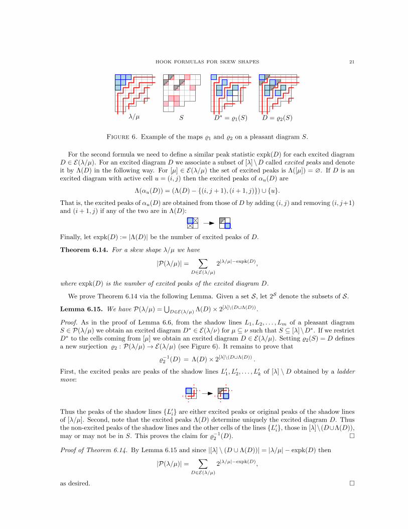
Proof of Proposition 6.12. As in the proof of Lemma 6.6, from the shadow lines L1, L2, . . . , Lm ofa pleasant diagram S ∈ P(λ/µ) we obtain an excited diagram D∗ ∈ E(λ/ν) for µ ⊆ ν such thatS ⊆ [λ]\D∗. The peaks of these lines are elements in S, and these peaks uniquely determine the lines.The other cells in the lines, |λ/ν| − shpk(D∗) many, may or may not be in S.
Therefore, we obtain a surjection
%1 : P(λ/µ)→⋃
ν,µ⊆ν⊆λE(λ/ν) , %1 : S 7→ D∗ ,
such that |%−11 (D∗)| = 2|λ/ν|−shpk(D∗). This implies the result (see Figure 6).
HOOK FORMULAS FOR SKEW SHAPES 21
S D∗ = %1(S)λ/µ D = %2(S)
Figure 6. Example of the maps %1 and %2 on a pleasant diagram S.
For the second formula we need to define a similar peak statistic expk(D) for each excited diagramD ∈ E(λ/µ). For an excited diagram D we associate a subset of [λ]\D called excited peaks and denoteit by Λ(D) in the following way. For [µ] ∈ E(λ/µ) the set of excited peaks is Λ([µ]) = ∅. If D is anexcited diagram with active cell u = (i, j) then the excited peaks of αu(D) are
Λ(αu(D)) = (Λ(D)− (i, j + 1), (i+ 1, j)) ∪ u.
That is, the excited peaks of αu(D) are obtained from those of D by adding (i, j) and removing (i, j+1)and (i+ 1, j) if any of the two are in Λ(D):
.
Finally, let expk(D) := |Λ(D)| be the number of excited peaks of D.
Theorem 6.14. For a skew shape λ/µ we have
|P(λ/µ)| =∑
D∈E(λ/µ)
2|λ/µ|−expk(D),
where expk(D) is the number of excited peaks of the excited diagram D.
We prove Theorem 6.14 via the following Lemma. Given a set S, let 2S denote the subsets of S.
Lemma 6.15. We have P(λ/µ) =⋃D∈E(λ/µ) Λ(D)× 2[λ]\(D∪Λ(D)).
Proof. As in the proof of Lemma 6.6, from the shadow lines L1, L2, . . . , Lm of a pleasant diagramS ∈ P(λ/µ) we obtain an excited diagram D∗ ∈ E(λ/ν) for µ ⊆ ν such that S ⊆ [λ]\D∗. If we restrictD∗ to the cells coming from [µ] we obtain an excited diagram D ∈ E(λ/µ). Setting %2(S) = D definesa new surjection %2 : P(λ/µ)→ E(λ/µ) (see Figure 6). It remains to prove that
%−12 (D) = Λ(D)× 2[λ]\(D∪Λ(D)) .
First, the excited peaks are peaks of the shadow lines L′1, L′2, . . . , L
′k of [λ] \D obtained by a ladder
move:
Thus the peaks of the shadow lines L′i are either excited peaks or original peaks of the shadow linesof [λ/µ]. Second, note that the excited peaks Λ(D) determine uniquely the excited diagram D. Thusthe non-excited peaks of the shadow lines and the other cells of the lines L′i, those in [λ]\(D∪Λ(D)),may or may not be in S. This proves the claim for %−1
2 (D).
Proof of Theorem 6.14. By Lemma 6.15 and since |[λ] \ (D ∪ Λ(D))| = |λ/µ| − expk(D) then
|P(λ/µ)| =∑
D∈E(λ/µ)
2|λ/µ|−expk(D),
as desired.
22 ALEJANDRO MORALES, IGOR PAK, GRETA PANOVA
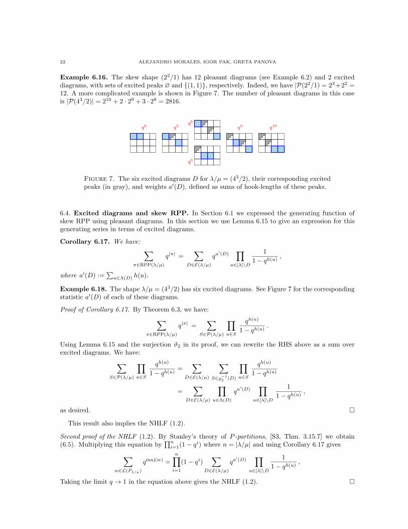
Example 6.16. The skew shape (22/1) has 12 pleasant diagrams (see Example 6.2) and 2 exciteddiagrams, with sets of excited peaks ∅ and (1, 1), respectively. Indeed, we have |P(22/1) = 23 +22 =12. A more complicated example is shown in Figure 7. The number of pleasant diagrams in this caseis |P(43/2)| = 210 + 2 · 29 + 3 · 28 = 2816.
q0 q5q8
q6
q9 q10
Figure 7. The six excited diagrams D for λ/µ = (43/2), their corresponding excitedpeaks (in gray), and weights a′(D), defined as sums of hook-lengths of these peaks.
6.4. Excited diagrams and skew RPP. In Section 6.1 we expressed the generating function ofskew RPP using pleasant diagrams. In this section we use Lemma 6.15 to give an expression for thisgenerating series in terms of excited diagrams.
Corollary 6.17. We have: ∑π∈RPP(λ/µ)
q|π| =∑
D∈E(λ/µ)
qa′(D)
∏u∈[λ]\D
1
1− qh(u),
where a′(D) :=∑u∈Λ(D) h(u).
Example 6.18. The shape λ/µ = (43/2) has six excited diagrams. See Figure 7 for the correspondingstatistic a′(D) of each of these diagrams.
Proof of Corollary 6.17. By Theorem 6.3, we have:∑π∈RPP(λ/µ)
q|π| =∑
S∈P(λ/µ)
∏u∈S
qh(u)
1− qh(u).
Using Lemma 6.15 and the surjection ϑ2 in its proof, we can rewrite the RHS above as a sum overexcited diagrams. We have:∑
S∈P(λ/µ)
∏u∈S
qh(u)
1− qh(u)=
∑D∈E(λ/µ)
∑S∈%−1
2 (D)
∏u∈S
qh(u)
1− qh(u)
=∑
D∈E(λ/µ)
∏u∈Λ(D)
qa′(D)
∏u∈[λ]\D
1
1− qh(u),
as desired.
This result also implies the NHLF (1.2).
Second proof of the NHLF (1.2). By Stanley’s theory of P -partitions, [S3, Thm. 3.15.7] we obtain(6.5). Multiplying this equation by
∏ni=1(1− qi) where n = |λ/µ| and using Corollary 6.17 gives∑
w∈L(Pλ/µ)
qmaj(w) =
n∏i=1
(1− qi)∑
D∈E(λ/µ)
qa′(D)
∏u∈[λ]\D
1
1− qh(u),
Taking the limit q → 1 in the equation above gives the NHLF (1.2).
HOOK FORMULAS FOR SKEW SHAPES 23
Corollary 6.19. We have:∑π∈RPP(λ/µ)
q|π| ttr(π) =∑
D∈E(λ/µ)
qa′(D) tc(D)
∏u∈D∩λ
1
1− tqh(u)
∏u∈D\λ
1
1− qh(u),
where D = [λ] \D, a′(D) =∑u∈Λ(D) h(u) and c(D) = |Λ(D) ∩λ|.
Proof. The proof follows verbatim to those of theorems 1.7, 1.8 and Corollary 6.17. The details arestraightforward.
7. Hillman-Grassl map on skew SSYT
In this section we show that the Hillman-Grassl map is a bijection between SSYT of skew shape andcertain arrays of nonnegative integers with support in the complement of excited diagrams and someforced nonzero entries. First, we describe these arrays and state the main result.
7.1. Excited arrays. We fix the skew shape λ/µ. Recall that for 1 ≤ t ≤ `(λ)− 1, dt(µ) denotes thediagonal (i, j) ∈ λ/µ | i − j = µt − t, where µt = 0 if `(µ) < t ≤ `(λ). Thus each row of µ is incorrespondence with a diagonal dt(µ). See Figure 8: Left.
Let Aµ be the array of shape λ with ones in each diagonal dt(µ) and zeros elsewhere. For [µ] ∈E(λ/µ), each active cell u = (i, j) of [µ] satisfies (Aµ)i+1,j = 0 and (Aµ)i+1,j+1 = 1.
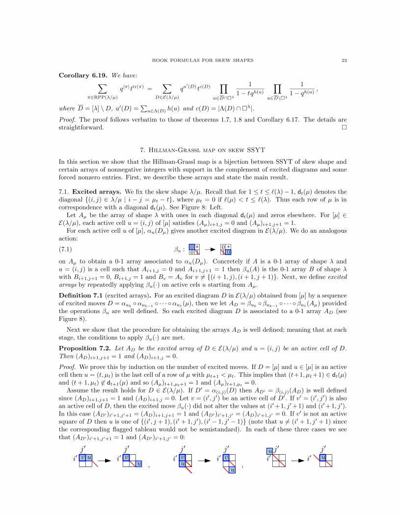
For each active cell u of [µ], αu(Dµ) gives another excited diagram in E(λ/µ). We do an analogousaction:
(7.1) βu : 11∗ ∗0
000
on Aµ to obtain a 0-1 array associated to αu(Dµ). Concretely if A is a 0-1 array of shape λ andu = (i, j) is a cell such that Ai+1,j = 0 and Ai+1,j+1 = 1 then βu(A) is the 0-1 array B of shape λwith Bi+1,j+1 = 0, Bi+1,j = 1 and Bv = Av for v 6= (i+ 1, j), (i+ 1, j + 1). Next, we define excitedarrays by repeatedly applying βu(·) on active cels u starting from Aµ.
Definition 7.1 (excited arrays). For an excited diagram D in E(λ/µ) obtained from [µ] by a sequenceof excited moves D = αuk αuk−1
· · · αu1(µ), then we let AD = βuk βuk−1 · · · βu1(Aµ) provided
the operations βu are well defined. So each excited diagram D is associated to a 0-1 array AD (seeFigure 8).
Next we show that the procedure for obtaining the arrays AD is well defined; meaning that at eachstage, the conditions to apply βu(·) are met.
Proposition 7.2. Let AD be the excited array of D ∈ E(λ/µ) and u = (i, j) be an active cell of D.Then (AD)i+1,j+1 = 1 and (AD)i+1,j = 0.
Proof. We prove this by induction on the number of excited moves. If D = [µ] and u ∈ [µ] is an activecell then u = (t, µt) is the last cell of a row of µ with µt+1 < µt. This implies that (t+1, µt+1) ∈ dt(µ)and (t+ 1, µt) 6∈ dt+1(µ) and so (Aµ)t+1,µt+1 = 1 and (Aµ)t+1,µt = 0.
Assume the result holds for D ∈ E(λ/µ). If D′ = α(i,j)(D) then AD′ = β(i,j)(AD) is well definedsince (AD)i+1,j+1 = 1 and (AD)i+1,j = 0. Let v = (i′, j′) be an active cell of D′. If v′ = (i′, j′) is alsoan active cell of D, then the excited move βu(·) did not alter the values at (i′+1, j′+1) and (i′+1, j′).In this case (AD′)i′+1,j′+1 = (AD)i+1,j+1 = 1 and (AD′)i′+1,j′ = (AD)i′+1,j′ = 0. If v′ is not an activesquare of D then u is one of (i′, j + 1), (i′ + 1, j′), (i′ − 1, j′ − 1) (note that u 6= (i′ + 1, j′ + 1) sincethe corresponding flagged tableau would not be semistandard). In each of these three cases we seethat (AD′)i′+1,j′+1 = 1 and (AD′)i′+1,j′ = 0:
vv u vuvuu
v
u
uu
, ,
j′
i′j′
i′j′
i′j′
i′j′
i′j′
i′
24 ALEJANDRO MORALES, IGOR PAK, GRETA PANOVA
d1(µ) d1(D)
Aµ AD
d1
A∅
µ
λ λ λ
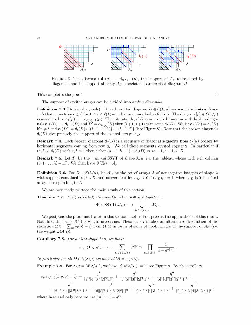
Figure 8. The diagonals d1(µ), . . . , d`(λ)−1(µ), the support of Aµ represented bydiagonals, and the support of array AD associated to an excited diagram D.
This completes the proof.
The support of excited arrays can be divided into broken diagonals
Definition 7.3 (Broken diagonals). To each excited diagram D ∈ E(λ/µ) we associate broken diago-nals that come from dt(µ) for 1 ≤ t ≤ `(λ)−1, that are described as follows. The diagram [µ] ∈ E(λ/µ)is associated to d1(µ), . . . , d`(λ)−1(µ). Then iteratively, if D is an excited diagram with broken diago-nals d1(D), . . . , d`−1(D) and D′ = α(i,j)(D) then (i+1, j+1) is in some dt(D). We let dr(D
′) = dr(D)if r 6= t and dt(D
′) = dt(D)\(i+1, j+1)∪(i+1, j) (See Figure 8). Note that the broken diagonalsdt(D) give precisely the support of the excited arrays AD.
Remark 7.4. Each broken diagonal dt(D) is a sequence of diagonal segments from dt(µ) broken byhorizontal segments coming from row µt. We call these segments excited segments. In particular if(a, b) ∈ dt(D) with a, b > 1 then either (a− 1, b− 1) ∈ dt(D) or (a− 1, b− 1) ∈ D.
Remark 7.5. Let T0 be the minimal SSYT of shape λ/µ, i.e. the tableau whose with i-th column(0, 1, . . . , λ′i − µ′i). We then have Φ(T0) = Aµ.
Definition 7.6. For D ∈ E(λ/µ), let A∗D be the set of arrays A of nonnegative integers of shape λwith support contained in [λ] \D, and nonzero entries Ai,j > 0 if (AD)i,j = 1, where AD is 0-1 excitedarray corresponding to D.
We are now ready to state the main result of this section.
Theorem 7.7. The (restricted) Hillman-Grassl map Φ is a bijection:
Φ : SSYT(λ/µ) −→⋃
D∈E(λ/µ)
A∗D .
We postpone the proof until later in this section. Let us first present the applications of this result.Note first that since Φ(·) is weight preserving, Theorem 7.7 implies an alternative description of thestatistic a(D) =
∑u∈D(λ′j − i) from (1.4) in terms of sums of hook-lengths of the support of AD (i.e.
the weight ω(AD)).
Corollary 7.8. For a skew shape λ/µ, we have:
sλ/µ(1, q, q2, . . .) =∑
D∈E(λ/µ)
qω(AD)∏
u∈[λ]\D
1
1− qh(u).
In particular for all D ∈ E(λ/µ) we have a(D) = ω(AD).
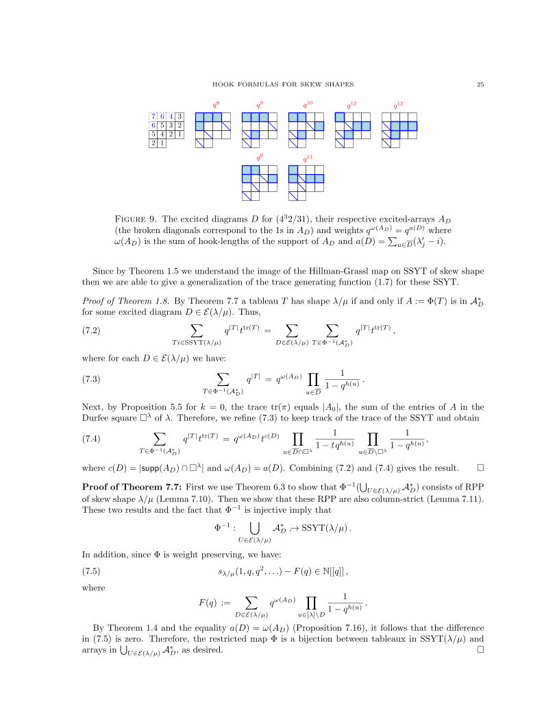
Example 7.9. For λ/µ = (432/31), we have |E(432/31)| = 7, see Figure 9. By the corollary,
s(432/31)(1, q, q2, . . .) =
q8
[5]2[4][3]2[2]3[1]2+
q9
[6][5]2[3]2[2]3[1]2+
q9
[5]2[4]2[3]2[2]2[1]2+
+q10
[6][5]2[4][3]2[2]2[1]2+
q11
[6][5]2[4]2[3][2]2[1]2+
q12
[6]2[5]2[4][3][2]2[1]2+
q13
[7][6]2[5][4][3][2]2[1]2,
where here and only here we use [m] := 1− qm.
HOOK FORMULAS FOR SKEW SHAPES 25
3423561245
67
q8 q9
12
q9
q10
q11
q12 q13
Figure 9. The excited diagrams D for (432/31), their respective excited-arrays AD(the broken diagonals correspond to the 1s in AD) and weights qω(AD) = qa(D) whereω(AD) is the sum of hook-lengths of the support of AD and a(D) =
∑u∈D(λ′j − i).
Since by Theorem 1.5 we understand the image of the Hillman-Grassl map on SSYT of skew shapethen we are able to give a generalization of the trace generating function (1.7) for these SSYT.
Proof of Theorem 1.8. By Theorem 7.7 a tableau T has shape λ/µ if and only if A := Φ(T ) is in A∗Dfor some excited diagram D ∈ E(λ/µ). Thus,
(7.2)∑
Ti∈SSYT(λ/µ)
q|T | ttr(T ) =∑
D∈E(λ/µ)
∑T∈Φ−1(A∗D)
q|T | ttr(T ) ,
where for each D ∈ E(λ/µ) we have:
(7.3)∑
T∈Φ−1(A∗D)
q|T | = qω(AD)∏u∈D
1
1− qh(u).
Next, by Proposition 5.5 for k = 0, the trace tr(π) equals |A0|, the sum of the entries of A in theDurfee square λ of λ. Therefore, we refine (7.3) to keep track of the trace of the SSYT and obtain
(7.4)∑
T∈Φ−1(A∗D)
q|T | ttr(T ) = qω(AD) tc(D)∏
u∈D∩λ
1
1− tqh(u)
∏u∈D\λ
1
1− qh(u),
where c(D) = |supp(AD) ∩λ| and ω(AD) = a(D). Combining (7.2) and (7.4) gives the result.
Proof of Theorem 7.7: First we use Theorem 6.3 to show that Φ−1(⋃U∈E(λ/µ)A∗D) consists of RPP
of skew shape λ/µ (Lemma 7.10). Then we show that these RPP are also column-strict (Lemma 7.11).These two results and the fact that Φ−1 is injective imply that
Φ−1 :⋃
U∈E(λ/µ)
A∗D → SSYT(λ/µ) .
In addition, since Φ is weight preserving, we have:
(7.5) sλ/µ(1, q, q2, . . .)− F (q) ∈ N[[q]] ,
where
F (q) :=∑
D∈E(λ/µ)
qω(AD)∏
u∈[λ]\D
1
1− qh(u).
By Theorem 1.4 and the equality a(D) = ω(AD) (Proposition 7.16), it follows that the differencein (7.5) is zero. Therefore, the restricted map Φ is a bijection between tableaux in SSYT(λ/µ) andarrays in
⋃U∈E(λ/µ)A∗D, as desired.
26 ALEJANDRO MORALES, IGOR PAK, GRETA PANOVA
7.2. Φ−1(A∗D) are RPP of skew shape. Given an excited diagram D ∈ E(λ/µ), let AD be the setof arrays of nonnegative integers of shape λ with support in [λ] \ D. Note that the set of excitedarrays A∗D from Definition 7.6 is contained in AD. We show that the RPP in Φ−1(AD) have supportcontained in λ/µ and therefore so do the RPP in Φ−1(A∗D).
Lemma 7.10. For each excited diagram D ∈ E(λ/µ), the reverse plane partitions in Φ−1(A∗D) havesupport contained in λ/µ.
Proof. By Lemma 6.7, the support of arrays inAD are pleasant diagrams in P(λ/µ). So by Theorem 6.3it follows that Φ−1(AD) ⊆ RPP(λ/µ). Since A∗D ⊆ AD, the result follows.
7.3. Φ−1(A∗D) are column strict skew RPP.
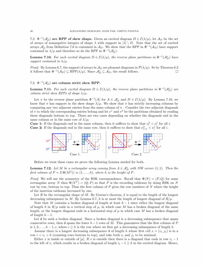
Lemma 7.11. For each excited diagram D ∈ E(λ/µ), the reverse plane partitions in Φ−1(A∗D) arecolumn strict skew RPPs of shape λ/µ.
Let π be the reverse plane partition Φ−1(A) for A ∈ A∗D and D ∈ E(λ/µ). By Lemma 7.10, weknow that π has support in the skew shape λ/µ. We show that π has strictly increasing columns bycomparing any two adjacent entries from the same column of π . Consider the two adjacent diagonalsof π to which the corresponding entries belong and let ν1 and ν2 be the partitions obtained by readingthese diagonals bottom to top. There are two cases depending on whether the diagonals end in thesame column or in the same row of λ/µ;Case 1: If the diagonals end in the same column, then it suffices to show that ν2
i < ν1i for all i.
Case 2: If the diagonals end in the same row, then it suffices to show that ν2i+1 < ν1
i for all i.
M2
M1 ν2
ν1ν2
ν1
Φ−1 Φ−1
M2
M1
Case 1. Case 2.
w
v
Before we treat these cases we prove the following Lemma needed for both.
Lemma 7.12. Let M be a rectangular array coming from A ∈ A∗D with NW corner (1, 1). Then the
first column of P = I(Ψ(Ml)) is (1, . . . , h), where h is the height of P .
Proof. We will use the symmetry of the RSK correspondence. Recall that Ψ(N) = (P,Q) for somerectangular array N then Ψ(NT ) = (Q,P ) so that P is the recording tableaux by doing RSK on Nrow by row, bottom to top. Thus the first column of P gives the row numbers of N where the heightof the insertion tableaux increased by one.
Let R be the rectangular shape of M . By Greene’s theorem, h is equal to the length of the longestdecreasing subsequence in M . By Lemma 6.7, h is at most the length of longest diagonal of R/µ.
Note that M contains a broken diagonal of length at least h − 1 since either the longest diagonalof length h in R/µ ends in a vertical step of µ, in which case M has a broken diagonal of the samelength, or the longest diagonal ends in a horizontal step of µ in which case M has a broken diagonalof length h− 1.
Let d be such a broken diagonal. Since a broken diagonal is a decreasing subsequence that spansconsecutive rows, then d spans the lower h− 1 rows of M . This guarantees that the first column of Pis 1, 2, . . . , h− 1, c, where c ≥ h is the row where we first get a decreasing subsequence of length h.
Assume there is a longest decreasing subsequence d of length h whose first cell x = (i1, j1) is in arow c = i1 > h (counting rows bottom to top), and take both i1 and j1 to be minimal.
Either x is inside or outside of [µ]. If x is outside then there is a diagonal that ends in row i1 − 1to the left of x, which results in a broken diagonal of length i1− 1 ≥ h in the excited diagram. Hence,
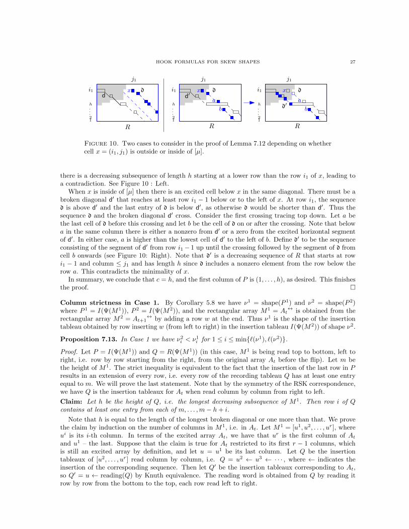
HOOK FORMULAS FOR SKEW SHAPES 27
R
a
b
xx
R R
a
b
xi1 i1
j1 j1
i1
j1
12
h
12
h
12
h
dd d d
d′
d′
Figure 10. Two cases to consider in the proof of Lemma 7.12 depending on whethercell x = (i1, j1) is outside or inside of [µ].
there is a decreasing subsequence of length h starting at a lower row than the row i1 of x, leading toa contradiction. See Figure 10 : Left.
When x is inside of [µ] then there is an excited cell below x in the same diagonal. There must be abroken diagonal d′ that reaches at least row i1 − 1 below or to the left of x. At row i1, the sequenced is above d′ and the last entry of d is below d′, as otherwise d would be shorter than d′. Thus thesequence d and the broken diagonal d′ cross. Consider the first crossing tracing top down. Let a bethe last cell of d before this crossing and let b be the cell of d on or after the crossing. Note that belowa in the same column there is either a nonzero from d′ or a zero from the excited horizontal segmentof d′. In either case, a is higher than the lowest cell of d′ to the left of b. Define d′ to be the sequenceconsisting of the segment of d′ from row i1− 1 up until the crossing followed by the segment of d fromcell b onwards (see Figure 10: Right). Note that d′ is a decreasing sequence of R that starts at rowi1 − 1 and column ≤ j1 and has length h since d includes a nonzero element from the row below therow a. This contradicts the minimality of x.
In summary, we conclude that c = h, and the first column of P is (1, . . . , h), as desired. This finishesthe proof.
Column strictness in Case 1. By Corollary 5.8 we have ν1 = shape(P 1) and ν2 = shape(P 2)where P 1 = I(Ψ(M1)), P 2 = I(Ψ(M2)), and the rectangular array M1 = At
↔ is obtained from therectangular array M2 = At+1
↔ by adding a row w at the end. Thus ν1 is the shape of the insertiontableau obtained by row inserting w (from left to right) in the insertion tableau I(Ψ(M2)) of shape ν2.
Proposition 7.13. In Case 1 we have ν2i < ν1
i for 1 ≤ i ≤ min`(ν1), `(ν2).
Proof. Let P = I(Ψ(M1)) and Q = R(Ψ(M1)) (in this case, M1 is being read top to bottom, left toright, i.e. row by row starting from the right, from the original array At before the flip). Let m bethe height of M1. The strict inequality is equivalent to the fact that the insertion of the last row in Presults in an extension of every row, i.e. every row of the recording tableau Q has at least one entryequal to m. We will prove the last statement. Note that by the symmetry of the RSK correspondence,we have Q is the insertion tableaux for At when read column by column from right to left.
Claim: Let h be the height of Q, i.e. the longest decreasing subsequence of M1. Then row i of Qcontains at least one entry from each of m, . . . ,m− h+ i.
Note that h is equal to the length of the longest broken diagonal or one more than that. We provethe claim by induction on the number of columns in M1, i.e. in At. Let M1 = [u1, u2, . . . , ur], whereui is its i-th column. In terms of the excited array At, we have that ur is the first column of Atand u1 – the last. Suppose that the claim is true for At restricted to its first r − 1 columns, whichis still an excited array by definition, and let u = u1 be its last column. Let Q be the insertiontableaux of [u2, . . . , ur] read column by column, i.e. Q = u2 ← u3 ← · · · , where ← indicates theinsertion of the corresponding sequence. Then let Q′ be the insertion tableaux corresponding to At,so Q′ = u ← reading(Q) by Knuth equivalence. The reading word is obtained from Q by reading itrow by row from the bottom to the top, each row read left to right.
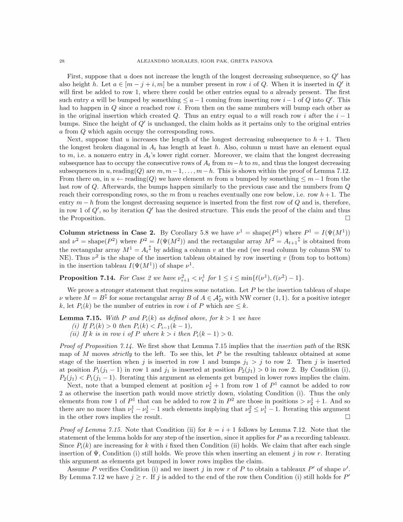
28 ALEJANDRO MORALES, IGOR PAK, GRETA PANOVA
First, suppose that u does not increase the length of the longest decreasing subsequence, so Q′ hasalso height h. Let a ∈ [m− j + i,m] be a number present in row i of Q. When it is inserted in Q′ itwill first be added to row 1, where there could be other entries equal to a already present. The firstsuch entry a will be bumped by something ≤ a− 1 coming from inserting row i− 1 of Q into Q′. Thishad to happen in Q since a reached row i. From then on the same numbers will bump each other asin the original insertion which created Q. Thus an entry equal to a will reach row i after the i − 1bumps. Since the height of Q′ is unchanged, the claim holds as it pertains only to the original entriesa from Q which again occupy the corresponding rows.
Next, suppose that u increases the length of the longest decreasing subsequence to h + 1. Thenthe longest broken diagonal in At has length at least h. Also, column u must have an element equalto m, i.e. a nonzero entry in At’s lower right corner. Moreover, we claim that the longest decreasingsubsequence has to occupy the consecutive rows of At from m−h to m, and thus the longest decreasingsubsequences in u, reading(Q) are m,m−1, . . . ,m−h. This is shown within the proof of Lemma 7.12.From there on, in u← reading(Q) we have element m from u bumped by something ≤ m−1 from thelast row of Q. Afterwards, the bumps happen similarly to the previous case and the numbers from Qreach their corresponding rows, so the m from u reaches eventually one row below, i.e. row h+ 1. Theentry m− h from the longest decreasing sequence is inserted from the first row of Q and is, therefore,in row 1 of Q′, so by iteration Q′ has the desired structure. This ends the proof of the claim and thusthe Proposition.
Column strictness in Case 2. By Corollary 5.8 we have ν1 = shape(P 1) where P 1 = I(Ψ(M1))
and ν2 = shape(P 2) where P 2 = I(Ψ(M2)) and the rectangular array M2 = At+1l is obtained from
the rectangular array M1 = Atl by adding a column v at the end (we read column by column SW to
NE). Thus ν2 is the shape of the insertion tableau obtained by row inserting v (from top to bottom)in the insertion tableau I(Ψ(M1)) of shape ν1.
Proposition 7.14. For Case 2 we have ν2i+1 < ν1
i for 1 ≤ i ≤ min`(ν1), `(ν2)− 1.
We prove a stronger statement that requires some notation. Let P be the insertion tableau of shapeν where M = Bl for some rectangular array B of A ∈ A∗D with NW corner (1, 1). for a positive integerk, let Pi(k) be the number of entries in row i of P which are ≤ k.
Lemma 7.15. With P and Pi(k) as defined above, for k > 1 we have(i) If Pi(k) > 0 then Pi(k) < Pi−1(k − 1),
(ii) If k is in row i of P where k > i then Pi(k − 1) > 0.
Proof of Proposition 7.14. We first show that Lemma 7.15 implies that the insertion path of the RSKmap of M moves strictly to the left. To see this, let P be the resulting tableaux obtained at somestage of the insertion when j is inserted in row 1 and bumps j1 > j to row 2. Then j is insertedat position P1(j1 − 1) in row 1 and j1 is inserted at position P2(j1) > 0 in row 2. By Condition (i),P2(j1) < P1(j1 − 1). Iterating this argument as elements get bumped in lower rows implies the claim.
Next, note that a bumped element at position ν12 + 1 from row 1 of P 1 cannot be added to row
2 as otherwise the insertion path would move strictly down, violating Condition (i). Thus the onlyelements from row 1 of P 1 that can be added to row 2 in P 2 are those in positions > ν1
2 + 1. And sothere are no more than ν1
1 − ν12 − 1 such elements implying that ν2
2 ≤ ν11 − 1. Iterating this argument
in the other rows implies the result.
Proof of Lemma 7.15. Note that Condition (ii) for k = i + 1 follows by Lemma 7.12. Note that thestatement of the lemma holds for any step of the insertion, since it applies for P as a recording tableaux.Since Pi(k) are increasing for k with i fixed then Condition (ii) holds. We claim that after each singleinsertion of Ψ, Condition (i) still holds. We prove this when inserting an element j in row r. Iteratingthis argument as elements get bumped in lower rows implies the claim.
Assume P verifies Condition (i) and we insert j in row r of P to obtain a tableaux P ′ of shape ν′.By Lemma 7.12 we have j ≥ r. If j is added to the end of the row then Condition (i) still holds for P ′
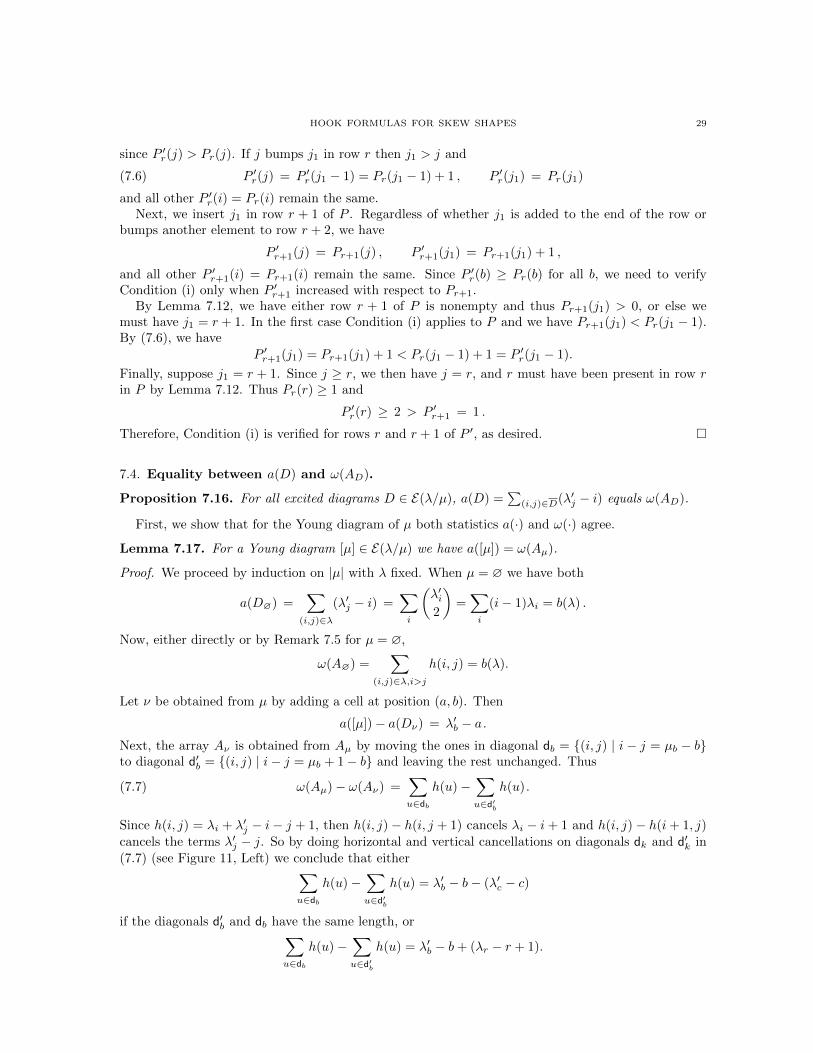
HOOK FORMULAS FOR SKEW SHAPES 29
since P ′r(j) > Pr(j). If j bumps j1 in row r then j1 > j and
(7.6) P ′r(j) = P ′r(j1 − 1) = Pr(j1 − 1) + 1 , P ′r(j1) = Pr(j1)
and all other P ′r(i) = Pr(i) remain the same.Next, we insert j1 in row r + 1 of P . Regardless of whether j1 is added to the end of the row or
bumps another element to row r + 2, we have
P ′r+1(j) = Pr+1(j) , P ′r+1(j1) = Pr+1(j1) + 1 ,
and all other P ′r+1(i) = Pr+1(i) remain the same. Since P ′r(b) ≥ Pr(b) for all b, we need to verifyCondition (i) only when P ′r+1 increased with respect to Pr+1.
By Lemma 7.12, we have either row r + 1 of P is nonempty and thus Pr+1(j1) > 0, or else wemust have j1 = r + 1. In the first case Condition (i) applies to P and we have Pr+1(j1) < Pr(j1 − 1).By (7.6), we have
P ′r+1(j1) = Pr+1(j1) + 1 < Pr(j1 − 1) + 1 = P ′r(j1 − 1).
Finally, suppose j1 = r + 1. Since j ≥ r, we then have j = r, and r must have been present in row rin P by Lemma 7.12. Thus Pr(r) ≥ 1 and
P ′r(r) ≥ 2 > P ′r+1 = 1 .
Therefore, Condition (i) is verified for rows r and r + 1 of P ′, as desired.
7.4. Equality between a(D) and ω(AD).
Proposition 7.16. For all excited diagrams D ∈ E(λ/µ), a(D) =∑
(i,j)∈D(λ′j − i) equals ω(AD).
First, we show that for the Young diagram of µ both statistics a(·) and ω(·) agree.
Lemma 7.17. For a Young diagram [µ] ∈ E(λ/µ) we have a([µ]) = ω(Aµ).
Proof. We proceed by induction on |µ| with λ fixed. When µ = ∅ we have both
a(D∅) =∑
(i,j)∈λ(λ′j − i) =
∑i
(λ′i2
)=∑i
(i− 1)λi = b(λ) .
Now, either directly or by Remark 7.5 for µ = ∅,
ω(A∅) =∑
(i,j)∈λ,i>jh(i, j) = b(λ).
Let ν be obtained from µ by adding a cell at position (a, b). Then
a([µ])− a(Dν) = λ′b − a.Next, the array Aν is obtained from Aµ by moving the ones in diagonal db = (i, j) | i− j = µb − bto diagonal d′b = (i, j) | i− j = µb + 1− b and leaving the rest unchanged. Thus
(7.7) ω(Aµ)− ω(Aν) =∑u∈db
h(u)−∑u∈d′b
h(u) .
Since h(i, j) = λi + λ′j − i− j + 1, then h(i, j)− h(i, j + 1) cancels λi − i+ 1 and h(i, j)− h(i+ 1, j)cancels the terms λ′j − j. So by doing horizontal and vertical cancellations on diagonals dk and d′k in(7.7) (see Figure 11, Left) we conclude that either∑
u∈dbh(u)−
∑u∈d′b
h(u) = λ′b − b− (λ′c − c)
if the diagonals d′b and db have the same length, or∑u∈db
h(u)−∑u∈d′b
h(u) = λ′b − b+ (λr − r + 1).
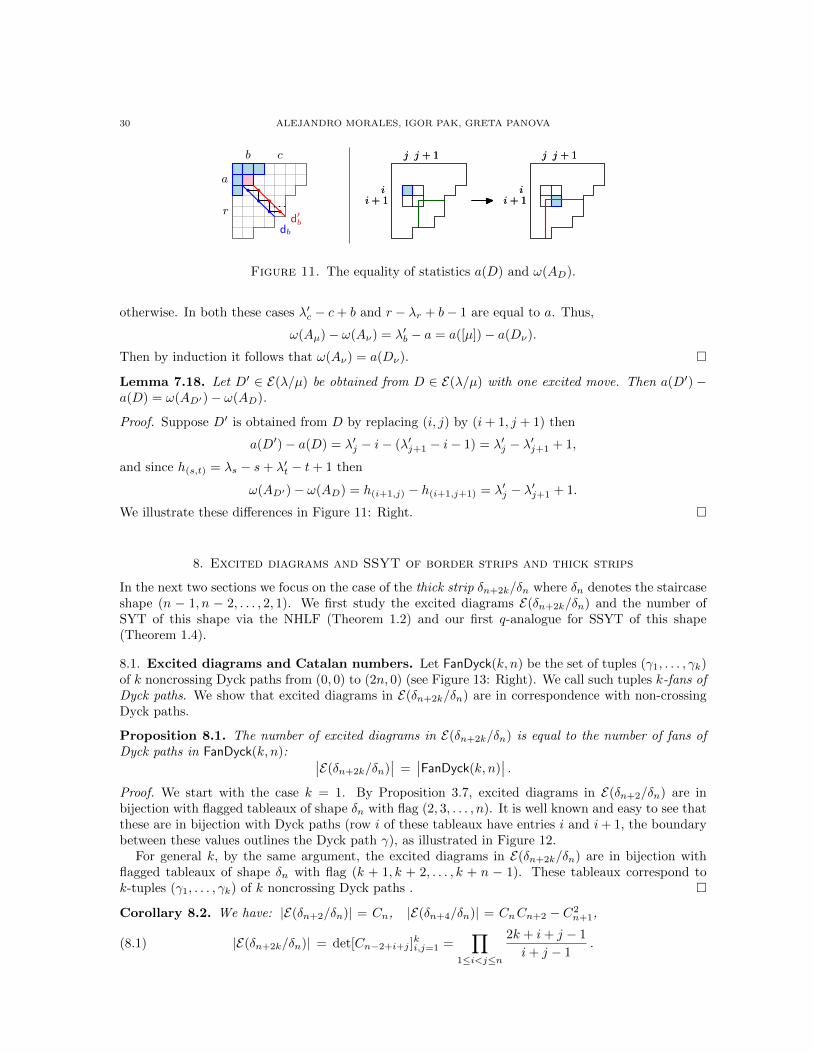
30 ALEJANDRO MORALES, IGOR PAK, GRETA PANOVA
ii+ 1
j j + 1
ii+ 1
j j + 1
ii+ 1
j j + 1
ii+ 1
j j + 1
a
b c
rd′b
db
Figure 11. The equality of statistics a(D) and ω(AD).
otherwise. In both these cases λ′c − c+ b and r − λr + b− 1 are equal to a. Thus,
ω(Aµ)− ω(Aν) = λ′b − a = a([µ])− a(Dν).
Then by induction it follows that ω(Aν) = a(Dν).
Lemma 7.18. Let D′ ∈ E(λ/µ) be obtained from D ∈ E(λ/µ) with one excited move. Then a(D′)−a(D) = ω(AD′)− ω(AD).
Proof. Suppose D′ is obtained from D by replacing (i, j) by (i+ 1, j + 1) then
a(D′)− a(D) = λ′j − i− (λ′j+1 − i− 1) = λ′j − λ′j+1 + 1,
and since h(s,t) = λs − s+ λ′t − t+ 1 then
ω(AD′)− ω(AD) = h(i+1,j) − h(i+1,j+1) = λ′j − λ′j+1 + 1.
We illustrate these differences in Figure 11: Right.
8. Excited diagrams and SSYT of border strips and thick strips
In the next two sections we focus on the case of the thick strip δn+2k/δn where δn denotes the staircaseshape (n − 1, n − 2, . . . , 2, 1). We first study the excited diagrams E(δn+2k/δn) and the number ofSYT of this shape via the NHLF (Theorem 1.2) and our first q-analogue for SSYT of this shape(Theorem 1.4).
8.1. Excited diagrams and Catalan numbers. Let FanDyck(k, n) be the set of tuples (γ1, . . . , γk)of k noncrossing Dyck paths from (0, 0) to (2n, 0) (see Figure 13: Right). We call such tuples k-fans ofDyck paths. We show that excited diagrams in E(δn+2k/δn) are in correspondence with non-crossingDyck paths.
Proposition 8.1. The number of excited diagrams in E(δn+2k/δn) is equal to the number of fans ofDyck paths in FanDyck(k, n): ∣∣E(δn+2k/δn)
∣∣ =∣∣FanDyck(k, n)
∣∣ .Proof. We start with the case k = 1. By Proposition 3.7, excited diagrams in E(δn+2/δn) are inbijection with flagged tableaux of shape δn with flag (2, 3, . . . , n). It is well known and easy to see thatthese are in bijection with Dyck paths (row i of these tableaux have entries i and i+ 1, the boundarybetween these values outlines the Dyck path γ), as illustrated in Figure 12.
For general k, by the same argument, the excited diagrams in E(δn+2k/δn) are in bijection withflagged tableaux of shape δn with flag (k + 1, k + 2, . . . , k + n − 1). These tableaux correspond tok-tuples (γ1, . . . , γk) of k noncrossing Dyck paths .
Corollary 8.2. We have: |E(δn+2/δn)| = Cn, |E(δn+4/δn)| = CnCn+2 − C2n+1,
(8.1) |E(δn+2k/δn)| = det[Cn−2+i+j ]ki,j=1 =
∏1≤i<j≤n
2k + i+ j − 1
i+ j − 1.
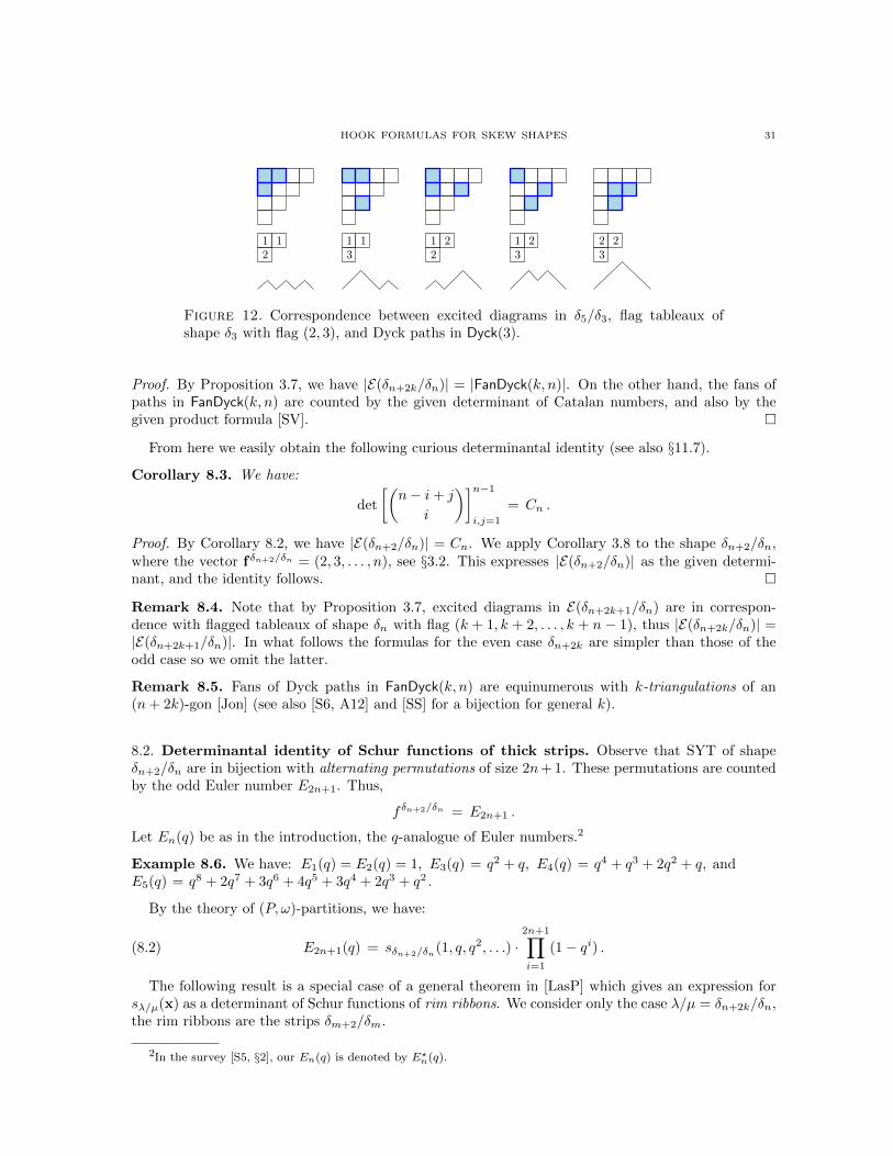
HOOK FORMULAS FOR SKEW SHAPES 31
1 12
1 13
1 22
1 23
2 23
Figure 12. Correspondence between excited diagrams in δ5/δ3, flag tableaux ofshape δ3 with flag (2, 3), and Dyck paths in Dyck(3).
Proof. By Proposition 3.7, we have |E(δn+2k/δn)| = |FanDyck(k, n)|. On the other hand, the fans ofpaths in FanDyck(k, n) are counted by the given determinant of Catalan numbers, and also by thegiven product formula [SV].
From here we easily obtain the following curious determinantal identity (see also §11.7).
Corollary 8.3. We have:
det
[(n− i+ j
i
)]n−1
i,j=1
= Cn .
Proof. By Corollary 8.2, we have |E(δn+2/δn)| = Cn. We apply Corollary 3.8 to the shape δn+2/δn,where the vector fδn+2/δn = (2, 3, . . . , n), see §3.2. This expresses |E(δn+2/δn)| as the given determi-nant, and the identity follows.
Remark 8.4. Note that by Proposition 3.7, excited diagrams in E(δn+2k+1/δn) are in correspon-dence with flagged tableaux of shape δn with flag (k + 1, k + 2, . . . , k + n − 1), thus |E(δn+2k/δn)| =|E(δn+2k+1/δn)|. In what follows the formulas for the even case δn+2k are simpler than those of theodd case so we omit the latter.
Remark 8.5. Fans of Dyck paths in FanDyck(k, n) are equinumerous with k-triangulations of an(n+ 2k)-gon [Jon] (see also [S6, A12] and [SS] for a bijection for general k).
8.2. Determinantal identity of Schur functions of thick strips. Observe that SYT of shapeδn+2/δn are in bijection with alternating permutations of size 2n+ 1. These permutations are countedby the odd Euler number E2n+1. Thus,
fδn+2/δn = E2n+1 .
Let En(q) be as in the introduction, the q-analogue of Euler numbers.2
Example 8.6. We have: E1(q) = E2(q) = 1, E3(q) = q2 + q, E4(q) = q4 + q3 + 2q2 + q, andE5(q) = q8 + 2q7 + 3q6 + 4q5 + 3q4 + 2q3 + q2 .
By the theory of (P, ω)-partitions, we have:
(8.2) E2n+1(q) = sδn+2/δn(1, q, q2, . . .) ·2n+1∏i=1
(1− qi) .
The following result is a special case of a general theorem in [LasP] which gives an expression forsλ/µ(x) as a determinant of Schur functions of rim ribbons. We consider only the case λ/µ = δn+2k/δn,the rim ribbons are the strips δm+2/δm.
2In the survey [S5, §2], our En(q) is denoted by E?n(q).
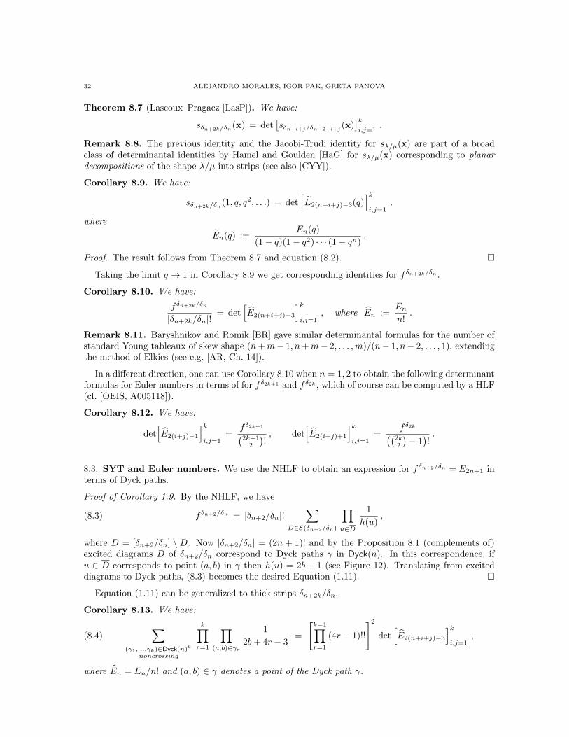
32 ALEJANDRO MORALES, IGOR PAK, GRETA PANOVA
Theorem 8.7 (Lascoux–Pragacz [LasP]). We have:
sδn+2k/δn(x) = det[sδn+i+j/δn−2+i+j
(x)]ki,j=1
.
Remark 8.8. The previous identity and the Jacobi-Trudi identity for sλ/µ(x) are part of a broadclass of determinantal identities by Hamel and Goulden [HaG] for sλ/µ(x) corresponding to planardecompositions of the shape λ/µ into strips (see also [CYY]).
Corollary 8.9. We have:
sδn+2k/δn(1, q, q2, . . .) = det[E2(n+i+j)−3(q)
]ki,j=1
,
where
En(q) :=En(q)
(1− q)(1− q2) · · · (1− qn).
Proof. The result follows from Theorem 8.7 and equation (8.2).
Taking the limit q → 1 in Corollary 8.9 we get corresponding identities for fδn+2k/δn .
Corollary 8.10. We have:
fδn+2k/δn
|δn+2k/δn|!= det
[E2(n+i+j)−3
]ki,j=1
, where En :=Enn!
.
Remark 8.11. Baryshnikov and Romik [BR] gave similar determinantal formulas for the number ofstandard Young tableaux of skew shape (n+m− 1, n+m− 2, . . . ,m)/(n− 1, n− 2, . . . , 1), extendingthe method of Elkies (see e.g. [AR, Ch. 14]).
In a different direction, one can use Corollary 8.10 when n = 1, 2 to obtain the following determinantformulas for Euler numbers in terms of for fδ2k+1 and fδ2k , which of course can be computed by a HLF(cf. [OEIS, A005118]).
Corollary 8.12. We have:
det[E2(i+j)−1
]ki,j=1
=fδ2k+1(2k+1
2
)!, det
[E2(i+j)+1
]ki,j=1
=fδ2k((
2k2
)− 1)!.
8.3. SYT and Euler numbers. We use the NHLF to obtain an expression for fδn+2/δn = E2n+1 interms of Dyck paths.
Proof of Corollary 1.9. By the NHLF, we have
(8.3) fδn+2/δn = |δn+2/δn|!∑
D∈E(δn+2/δn)
∏u∈D
1
h(u),
where D = [δn+2/δn] \ D. Now |δn+2/δn| = (2n + 1)! and by the Proposition 8.1 (complements of)excited diagrams D of δn+2/δn correspond to Dyck paths γ in Dyck(n). In this correspondence, ifu ∈ D corresponds to point (a, b) in γ then h(u) = 2b + 1 (see Figure 12). Translating from exciteddiagrams to Dyck paths, (8.3) becomes the desired Equation (1.11).
Equation (1.11) can be generalized to thick strips δn+2k/δn.
Corollary 8.13. We have:
(8.4)∑
(γ1,...,γk)∈Dyck(n)k
noncrossing
k∏r=1
∏(a,b)∈γr
1
2b+ 4r − 3=
[k−1∏r=1
(4r − 1)!!
]2
det[E2(n+i+j)−3
]ki,j=1
,
where En = En/n! and (a, b) ∈ γ denotes a point of the Dyck path γ.
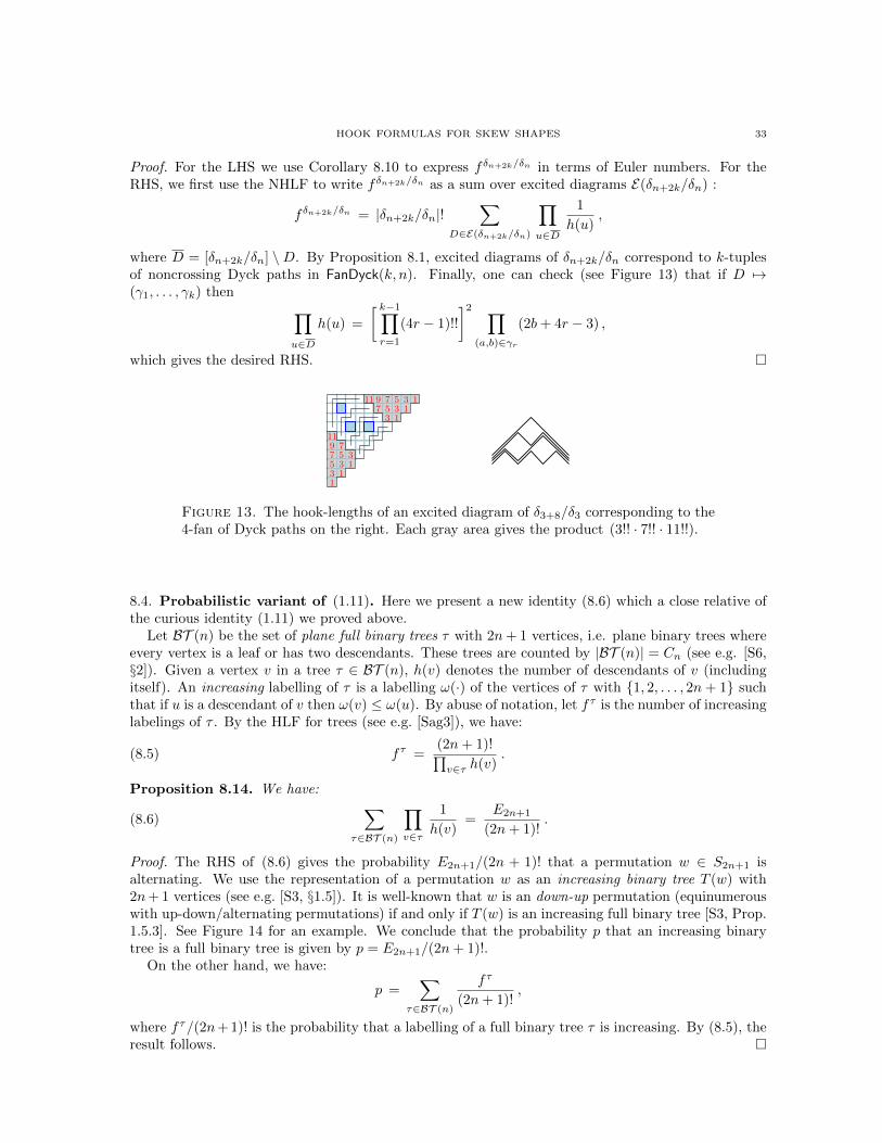
HOOK FORMULAS FOR SKEW SHAPES 33
Proof. For the LHS we use Corollary 8.10 to express fδn+2k/δn in terms of Euler numbers. For theRHS, we first use the NHLF to write fδn+2k/δn as a sum over excited diagrams E(δn+2k/δn) :
fδn+2k/δn = |δn+2k/δn|!∑
D∈E(δn+2k/δn)
∏u∈D
1
h(u),
where D = [δn+2k/δn] \D. By Proposition 8.1, excited diagrams of δn+2k/δn correspond to k-tuplesof noncrossing Dyck paths in FanDyck(k, n). Finally, one can check (see Figure 13) that if D 7→(γ1, . . . , γk) then ∏
u∈Dh(u) =
[ k−1∏r=1
(4r − 1)!!
]2 ∏(a,b)∈γr
(2b+ 4r − 3) ,
which gives the desired RHS.
13
31
13
11
1
33
35
577911
557
7911
Figure 13. The hook-lengths of an excited diagram of δ3+8/δ3 corresponding to the4-fan of Dyck paths on the right. Each gray area gives the product (3!! · 7!! · 11!!).
8.4. Probabilistic variant of (1.11). Here we present a new identity (8.6) which a close relative ofthe curious identity (1.11) we proved above.
Let BT (n) be the set of plane full binary trees τ with 2n+ 1 vertices, i.e. plane binary trees whereevery vertex is a leaf or has two descendants. These trees are counted by |BT (n)| = Cn (see e.g. [S6,§2]). Given a vertex v in a tree τ ∈ BT (n), h(v) denotes the number of descendants of v (includingitself). An increasing labelling of τ is a labelling ω(·) of the vertices of τ with 1, 2, . . . , 2n+ 1 suchthat if u is a descendant of v then ω(v) ≤ ω(u). By abuse of notation, let fτ is the number of increasinglabelings of τ . By the HLF for trees (see e.g. [Sag3]), we have:
(8.5) fτ =(2n+ 1)!∏v∈τ h(v)
.
Proposition 8.14. We have:
(8.6)∑
τ∈BT (n)
∏v∈τ
1
h(v)=
E2n+1
(2n+ 1)!.
Proof. The RHS of (8.6) gives the probability E2n+1/(2n + 1)! that a permutation w ∈ S2n+1 isalternating. We use the representation of a permutation w as an increasing binary tree T (w) with2n+ 1 vertices (see e.g. [S3, §1.5]). It is well-known that w is an down-up permutation (equinumerouswith up-down/alternating permutations) if and only if T (w) is an increasing full binary tree [S3, Prop.1.5.3]. See Figure 14 for an example. We conclude that the probability p that an increasing binarytree is a full binary tree is given by p = E2n+1/(2n+ 1)!.
On the other hand, we have:
p =∑
τ∈BT (n)
fτ
(2n+ 1)!,
where fτ/(2n+ 1)! is the probability that a labelling of a full binary tree τ is increasing. By (8.5), theresult follows.
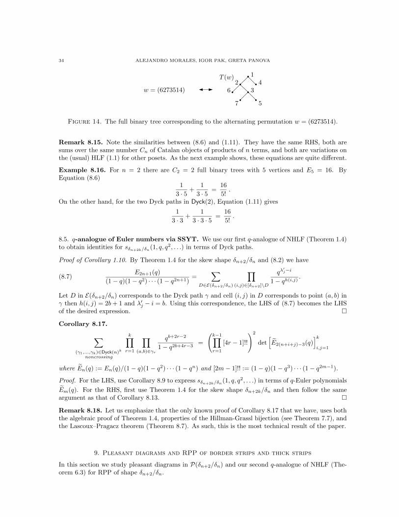
34 ALEJANDRO MORALES, IGOR PAK, GRETA PANOVA
w = (6273514)
12
6 3
7 5
4T (w)
Figure 14. The full binary tree corresponding to the alternating permutation w = (6273514).
Remark 8.15. Note the similarities between (8.6) and (1.11). They have the same RHS, both aresums over the same number Cn of Catalan objects of products of n terms, and both are variations onthe (usual) HLF (1.1) for other posets. As the next example shows, these equations are quite different.
Example 8.16. For n = 2 there are C2 = 2 full binary trees with 5 vertices and E5 = 16. ByEquation (8.6)
1
3 · 5+
1
3 · 5=
16
5!.
On the other hand, for the two Dyck paths in Dyck(2), Equation (1.11) gives
1
3 · 3+
1
3 · 3 · 5=
16
5!.
8.5. q-analogue of Euler numbers via SSYT. We use our first q-analogue of NHLF (Theorem 1.4)to obtain identities for sδn+2k/δn(1, q, q2, . . .) in terms of Dyck paths.
Proof of Corollary 1.10. By Theorem 1.4 for the skew shape δn+2/δn and (8.2) we have
(8.7)E2n+1(q)
(1− q)(1− q2) · · · (1− q2n+1)=
∑D∈E(δn+2/δn)
∏(i,j)∈[δn+2]\D
qλ′j−i
1− qh(i,j).
Let D in E(δn+2/δn) corresponds to the Dyck path γ and cell (i, j) in D corresponds to point (a, b) inγ then h(i, j) = 2b+ 1 and λ′j − i = b. Using this correspondence, the LHS of (8.7) becomes the LHSof the desired expression.
Corollary 8.17.
∑(γ1,...,γk)∈Dyck(n)k
noncrossing
k∏r=1
∏(a,b)∈γr
qb+2r−2
1− q2b+4r−3=
(k−1∏r=1
[4r − 1]!!
)2
det[E2(n+i+j)−3(q)
]ki,j=1
where En(q) := En(q)/(1− q)(1− q2) · · · (1− qn) and [2m− 1]!! := (1− q)(1− q3) · · · (1− q2m−1).
Proof. For the LHS, use Corollary 8.9 to express sδn+2k/δn(1, q, q2, . . .) in terms of q-Euler polynomials
Em(q). For the RHS, first use Theorem 1.4 for the skew shape δn+2k/δn and then follow the sameargument as that of Corollary 8.13.
Remark 8.18. Let us emphasize that the only known proof of Corollary 8.17 that we have, uses boththe algebraic proof of Theorem 1.4, properties of the Hillman-Grassl bijection (see Theorem 7.7), andthe Lascoux–Pragacz theorem (Theorem 8.7). As such, this is the most technical result of the paper.
9. Pleasant diagrams and RPP of border strips and thick strips
In this section we study pleasant diagrams in P(δn+2/δn) and our second q-analogue of NHLF (The-orem 6.3) for RPP of shape δn+2/δn.
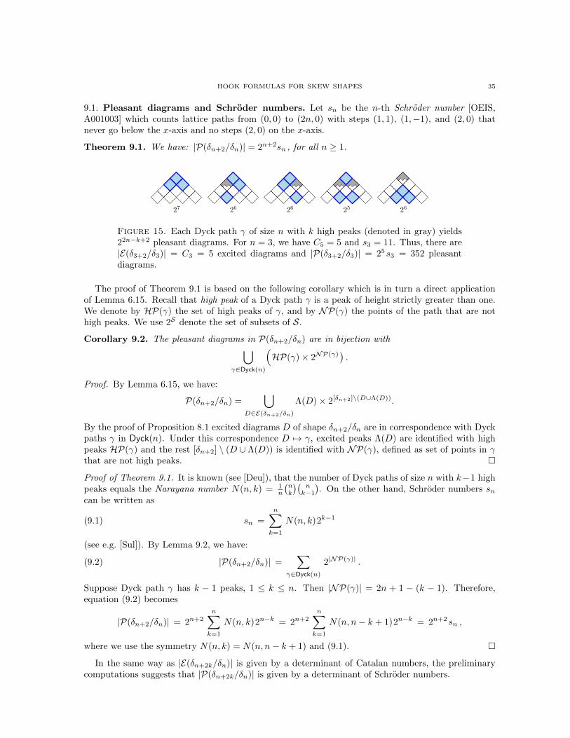
HOOK FORMULAS FOR SKEW SHAPES 35
9.1. Pleasant diagrams and Schroder numbers. Let sn be the n-th Schroder number [OEIS,A001003] which counts lattice paths from (0, 0) to (2n, 0) with steps (1, 1), (1,−1), and (2, 0) thatnever go below the x-axis and no steps (2, 0) on the x-axis.
Theorem 9.1. We have: |P(δn+2/δn)| = 2n+2sn , for all n ≥ 1.
27 26 26 25 26
Figure 15. Each Dyck path γ of size n with k high peaks (denoted in gray) yields22n−k+2 pleasant diagrams. For n = 3, we have C5 = 5 and s3 = 11. Thus, there are|E(δ3+2/δ3)| = C3 = 5 excited diagrams and |P(δ3+2/δ3)| = 25s3 = 352 pleasantdiagrams.
The proof of Theorem 9.1 is based on the following corollary which is in turn a direct applicationof Lemma 6.15. Recall that high peak of a Dyck path γ is a peak of height strictly greater than one.We denote by HP(γ) the set of high peaks of γ, and by NP(γ) the points of the path that are nothigh peaks. We use 2S denote the set of subsets of S.
Corollary 9.2. The pleasant diagrams in P(δn+2/δn) are in bijection with⋃γ∈Dyck(n)
(HP(γ)× 2NP(γ)
).
Proof. By Lemma 6.15, we have:
P(δn+2/δn) =⋃
D∈E(δn+2/δn)
Λ(D)× 2[δn+2]\(D∪Λ(D)).
By the proof of Proposition 8.1 excited diagrams D of shape δn+2/δn are in correspondence with Dyckpaths γ in Dyck(n). Under this correspondence D 7→ γ, excited peaks Λ(D) are identified with highpeaks HP(γ) and the rest [δn+2] \ (D ∪ Λ(D)) is identified with NP(γ), defined as set of points in γthat are not high peaks.
Proof of Theorem 9.1. It is known (see [Deu]), that the number of Dyck paths of size n with k−1 highpeaks equals the Narayana number N(n, k) = 1
n
(nk
)(nk−1
). On the other hand, Schroder numbers sn
can be written as
(9.1) sn =
n∑k=1
N(n, k)2k−1
(see e.g. [Sul]). By Lemma 9.2, we have:
(9.2) |P(δn+2/δn)| =∑
γ∈Dyck(n)
2|NP(γ)| .
Suppose Dyck path γ has k − 1 peaks, 1 ≤ k ≤ n. Then |NP(γ)| = 2n + 1 − (k − 1). Therefore,equation (9.2) becomes
|P(δn+2/δn)| = 2n+2n∑k=1
N(n, k)2n−k = 2n+2n∑k=1
N(n, n− k + 1)2n−k = 2n+2sn ,
where we use the symmetry N(n, k) = N(n, n− k + 1) and (9.1).
In the same way as |E(δn+2k/δn)| is given by a determinant of Catalan numbers, the preliminarycomputations suggests that |P(δn+2k/δn)| is given by a determinant of Schroder numbers.
36 ALEJANDRO MORALES, IGOR PAK, GRETA PANOVA
Conjecture 9.3. We have: |P(δn+4/δn)| = 22n+5(snsn+2 − s2n+1). More generally, for all k ≥ 1,
we have:|P(δn+2k/δn)| = 2(k2) det
[sn−2+i+j
]ki,j=1
, where sn = 2n+2sn .
Here we use sn = |P(δn+2/δn)| in place of sn in the determinant to make the formula more elegant.In fact, the power of 2 can be factored out.
9.2. q-analogue of Euler numbers via RPP. We use our second q-analogue of the NHLF (Theo-rem 1.5) and Lemma 9.2 to obtain identities for the generating function of RPP of shape δn+2/δn interms of Dyck paths. Recall the definition of E∗n(q) from the introduction:
E∗n(q) =∑
σ∈Alt(n)
qmaj(σ−1κ) ,
where κ = (13254 . . .). Note that maj(σκ) is the sum of the descents of σ ∈ Sn not involving both2i+ 1 and 2i.
Example 9.4. To complement Example 8.6, we have: E∗1 (q) = E∗2 (q) = 1, E∗3 (q) = q + 1,E∗4 (q) = q4 + q3 + q2 + q + 1, and E∗5 (q) = q7 + 2q6 + 2q5 + 3q4 + 3q3 + 2q2 + 2q + 1.
Proof of Corollary 1.11. By the theory of P -partitions, see (6.5), the generating series of RPP of shapeδn+2/δn equals ∑
π∈RPP(δn+2/δn)
q|π| =
∑u∈L(Pδn+2/δn
) qmaj(u)
(1− q)(1− q2) · · · (1− q2n+1),
where the sum in the numerator is over linear extensions L(Pδn+2/δn) of the zigzag poset Pδn+2/δn
with a natural labelling. These linear extensions are in bijection with alternating permutations of size2n+ 1 and
E∗2n+1(q) =∑
σ∈Alt2n+1
qmaj(σ−1κ) =∑
u∈L(Pδn+2/δn)
qmaj(u) .
Thus
(9.3)∑
π∈RPP(δn+2/δn)
q|π| =E∗2n+1(q)
(1− q)(1− q2) · · · (1− q2n+1).
By Corollary 6.17 for the skew shape δn+2/δn and (9.3), we have:
(9.4)∑
D∈E(δn+2/δn)
qa′(D)
∏u∈[λ]\D
1
1− qh(u)=
E∗2n+1(q)
(1− q)(1− q2) · · · (1− q2n+1),
where a′(D) =∑u∈Λ(D) h(u). By the proof of Lemma 9.2, if D ∈ E(δn+2/δn) corresponds to the Dyck
path γ then excited peaks u ∈ Λ(D) correspond to high peaks (c, d) ∈ HP(γ) and h(u) = 2d + 1.Using this correspondence, the LHS of (9.4) becomes the LHS of the desired expression.
Finally, preliminary computations suggest the following analogue of Corollary 8.9.
Conjecture 9.5. We have: ∑π∈RPP(δn+2k/δn)
q|π| = q−N det[E∗2(n+i+j)−3(q)
]ki,j=1
,
where N = k(k − 1)(6n+ 8k − 1)/6 and E∗k(q) = E∗k(q)/(1− q) · · · (1− qk) .
10. Other formulas for the number of standard Young tableaux
In this section we give a quick review of several competing formulas for computing fλ/µ.
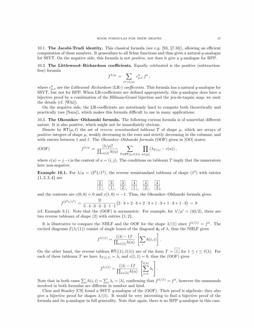
HOOK FORMULAS FOR SKEW SHAPES 37
10.1. The Jacobi-Trudi identity. This classical formula (see e.g. [S3, §7.16]), allowing an efficientcomputation of these numbers. It generalizes to all Schur functions and thus gives a natural q-analoguefor SSYT. On the negative side, this formula is not positive, nor does it give a q-analogue for RPP.
10.2. The Littlewood–Richardson coefficients. Equally celebrated is the positive (subtraction-free) formula
fλ/µ =∑
ν`|λ/µ|cλµ,ν f
ν ,
where cλµ,ν are the Littlewood–Richardson (LR-) coefficients. This formula has a natural q-analogue forSSYT, but not for RPP. When LR-coefficients are defined appropriately, this q-analogue does have abijective proof by a combination of the Hillman-Grassl bijection and the jeu-de-taquin map; we omitthe details (cf. [Whi]).
On the negative side, the LR-coefficients are notoriously hard to compute both theoretically andpractically (see [Nara]), which makes this formula difficult to use in many applications.
10.3. The Okounkov–Olshanski formula. The following curious formula is of somewhat differentnature. It is also positive, which might not be immediately obvious.
Denote by RT(µ, `) the set of reverse semistandard tableaux T of shape µ, which are arrays ofpositive integers of shape µ, weakly decreasing in the rows and strictly decreasing in the columns, andwith entries between 1 and `. The Okounkov–Olshanski formula (OOF) given in [OO] states:
(OOF) fλ/µ =|λ/µ|!∏u∈[λ] h(u)
∑T∈RT(µ,`(λ))
∏u∈[µ]
(λT (u) − c(u)) ,
where c(u) = j−i is the content of u = (i, j). The conditions on tableaux T imply that the numeratorshere non-negative.
Example 10.1. For λ/µ = (231/12), the reverse semistandard tableaux of shape (12) with entries1, 2, 3, 4 are
21 ,
31 ,
32 ,
41 ,
42 ,
43 ;
and the contents are c(0, 0) = 0 and c(1, 0) = −1. Thus, the Okounkov–Olshanski formula gives:
f (231/12) =5!
5 · 4 · 3 · 3 · 2 · 1 · 1(2 · 3 + 2 · 3 + 2 · 3 + 1 · 3 + 1 · 3 + 1 · 3
)= 9
(cf. Example 3.1). Note that the (OOF) is asymmetric. For example, for λ′/µ′ = (43/2), there aretwo reverse tableaux of shape (2) with entries 1, 2.
It is illustrative to compare the NHLF and the OOF for the shape λ/(1) since fλ/(1) = fλ. Theexcited diagrams E(λ/(1)) consist of single boxes of the diagonal d0 of λ, thus the NHLF gives
fλ/(1) =(|λ| − 1)!∏u∈[λ] h(u)
[∑i
h(i, i)
].
On the other hand, the reverse tableau RT((1), `(λ)) are of the form T = i for 1 ≤ i ≤ `(λ). Foreach of these tableaux T we have λT (1,1) = λi and c(1, 1) = 0, thus the (OOF) gives
fλ/(1) =(|λ| − 1)!∏u∈[λ] h(u)
`(λ)∑i=1
λi
.Note that in both cases
∑i h(i, i) =
∑i λi = |λ|, confirming that fλ/(1) = fλ, however the summands
involved in both formulas are different in number and kind.Chen and Stanley [CS] found a SSYT q-analogue of the (OOF). Their proof is algebraic; they also
give a bijective proof for shapes λ/(1). It would be very interesting to find a bijective proof of theformula and its q-analogue in full generality. Note that again, there is no RPP q-analogue in this case.
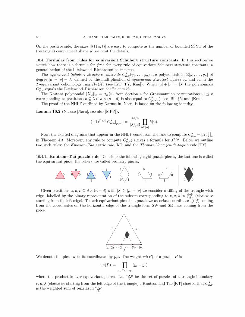
38 ALEJANDRO MORALES, IGOR PAK, GRETA PANOVA
On the positive side, the sizes |RT(µ, `)| are easy to compute as the number of bounded SSYT of the(rectangle) complement shape µ; we omit the details.
10.4. Formulas from rules for equivariant Schubert structure constants. In this section wesketch how there is a formula for fλ/µ for every rule of equivariant Schubert structure constants, ageneralization of the Littlewood–Richardson coefficients.
The equivariant Schubert structure constants Cλµ,ν(y1, . . . , yn) are polynomials in Z[y1, . . . , yn] ofdegree |µ| + |ν| − |λ| defined by the multiplication of equivariant Schubert classes σµ and σν in theT -equivariant cohomology ring HT (X) (see [KT, TY, Knu]). When |µ| + |ν| = |λ| the polynomialsCλµ,ν equals the Littlewood–Richardson coefficients cλµ,ν .
The Kostant polynomial [Xw]|v = σw(v) from Section 4 for Grassmannian permutations w vcorresponding to partitions µ ⊆ λ ⊂ d× (n− d) is also equal to Cλµ,λ(·), see [Bil, §5] and [Knu].
The proof of the NHLF outlined by Naruse in [Naru] is based on the following identity.
Lemma 10.2 (Naruse [Naru], see also [MPP]).
(−1)|λ/µ| Cλµ,λ|yi=i =fλ/µ
|λ/µ|!∏u∈[λ]
h(u).
Now, the excited diagrams that appear in the NHLF come from the rule to compute Cλµ,λ = [Xw]∣∣v
in Theorem 4.3. Moreover, any rule to compute Cλµ,ν(·) gives a formula for fλ/µ. Below we outlinetwo such rules: the Knutson–Tao puzzle rule [KT] and the Thomas–Yong jeu-de-taquin rule [TY].
10.4.1. Knutson–Tao puzzle rule. Consider the following eight puzzle pieces, the last one is calledthe equivariant piece, the others are called ordinary pieces:
0 0
0
0
0 0 1 1
1
1
1 1
1
10
0 0
1
0
1 0 0
1
1
0 1
1 0
Given partitions λ, µ, ν ⊆ d× (n− d) with |λ| ≥ |µ|+ |ν| we consider a tilling of the triangle with
edges labelled by the binary representation of the subsets corresponding to ν, µ, λ in(
[n]d
)(clockwise
starting from the left edge). To each equivariant piece in a puzzle we associate coordinates (i, j) comingfrom the coordinates on the horizontal edge of the triangle form SW and SE lines coming from thepiece:
y1 y2 . . . ynyjyi. . . . . .
ν µ
λ
We denote the piece with its coordinates by pij . The weight wt(P ) of a puzzle P is
wt(P ) =∏
pij∈P ; eq.
(yi − yj),
where the product is over equivariant pieces. Let ν∆µ
λbe the set of puzzles of a triangle boundary
ν, µ, λ (clockwise starting from the left edge of the triangle) . Knutson and Tao [KT] showed that Cλµ,νis the weighted sum of puzzles in ν∆µ
λ.
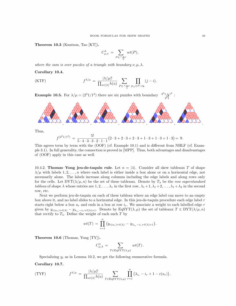
HOOK FORMULAS FOR SKEW SHAPES 39
Theorem 10.3 (Knutson, Tao [KT]).
Cλµ,ν =∑
P∈ ν∆µ
λ
wt(P ),
where the sum is over puzzles of a triangle with boundary ν, µ, λ.
Corollary 10.4.
(KTF) fλ/µ =|λ/µ|!∏u∈[λ] h(u)
∑P∈ λ∆µ
λ
∏pij∈P ; eq.
(j − i).
Example 10.5. For λ/µ = (231/12) there are six puzzles with boundary 231∆12
231:
000
000 0
00
000 0
00 0 1
1 0 000 0 1 0
00
000 1
11
01 0
00 0
00
111
01 1
11
01
01
01
,
000
000 0
00
000 0
00 0 1
1 0 0 101 0
00
000 1
11 0
00 0
00 0
00
111
01 1
11
01
01
01
,
000
000 0
00
000 0 1
01
1 0 0 1 000 0
00
000 1
11 0
00 0
00 0
00
111
01 1
11
01
01
01
,
000
000 0
00
000 0
00 0 1
111
01
01 0
00
0 1 1 0 000 0
00 0
00
111 0
00 1
11
01
01
01
,
000
000 0
00
000 0 1
01
111
01 0
00 0
00
0 1 1 0 000 0
00 0
00
111 0
00 1
11
01
01
01
,
000
000 0
00
0 101
01
111 0
00 0
00 0
00
0 1 1 0 000 0
00 0
00
111 0
00 1
11
01
01
01
.
Thus,
f (231/12) =5!
5 · 4 · 3 · 3 · 2 · 1 · 1(2 · 3 + 2 · 3 + 2 · 3 + 1 · 3 + 1 · 3 + 1 · 3
)= 9 .
This agrees term by term with the (OOF) (cf. Example 10.1) and is different from NHLF (cf. Exam-ple 3.1). In full generality, the connection is proved in [MPP]. Thus, both advantages and disadvantagesof (OOF) apply in this case as well.
10.4.2. Thomas–Yong jeu-de-taquin rule. Let n = |λ|. Consider all skew tableaux T of shapeλ/µ with labels 1, 2, . . . , n where each label is either inside a box alone or on a horizontal edge, notnecessarily alone. The labels increase along columns including the edge labels and along rows onlyfor the cells. Let DYT(λ/µ, n) be the set of these tableaux. Denote by Tλ be the row superstandardtableau of shape λ whose entries are 1, 2, . . . , λ1 in the first row, λ1 +1, λ1 +2, . . . , λ1 +λ2 in the secondrow, etc.
Next we perform jeu-de-taquin on each of these tableau where an edge label can move to an emptybox above it, and no label slides to a horizontal edge. In this jeu-de-taquin procedure each edge label rstarts right below a box ur and ends in a box at row ir. We associate a weight to each labelled edge rgiven by yc(ur)+`(λ) − yλir−ir+`(λ)+1. Denote by EqSYT(λ, µ) the set of tableaux T ∈ DYT(λ/µ, n)that rectify to Tλ. Define the weight of each such T by
wt(T ) =
n∏r=1
(yc(ur)+`(λ) − yλir−ir+`(λ)+1
).
Theorem 10.6 (Thomas, Yong [TY]).
Cλµ,λ =∑
T∈EqSYT(λ,µ)
wt(T ) .
Specializing yi as in Lemma 10.2, we get the following enumerative formula.
Corollary 10.7.
(TYF) fλ/µ =|λ/µ|!∏u∈[λ] h(u)
∑T∈EqSYT(λ,µ)
n∏r=1
(λir − ir + 1− c(ur)
).
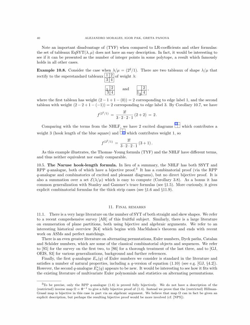
40 ALEJANDRO MORALES, IGOR PAK, GRETA PANOVA
Note an important disadvantage of (TYF) when compared to LR-coefficients and other formulas:the set of tableaux EqSYT(λ, µ) does not have an easy description. In fact, it would be interesting tosee if it can be presented as the number of integer points in some polytope, a result which famouslyholds in all other cases.
Example 10.8. Consider the case when λ/µ = (22/1). There are two tableaux of shape λ/µ that
rectify to the superstandard tableaux 1 23 4
of weight λ:
1 23 4
and 213 4
,
where the first tableau has weight (2− 1 + 1− (0)) = 2 corresponding to edge label 1, and the secondtableau with weight (2− 2 + 1− (−1)) = 2 corresponding to edge label 3. By Corollary 10.7, we have
f (22/1) =3!
3 · 2 · 2 · 1(2 + 2) = 2 .
Comparing with the terms from the NHLF, we have 2 excited diagrams which contributes a
weight 3 (hook length of the blue square) and which contributes weight 1, so
f (22/1) =3!
3 · 2 · 2 · 1(3 + 1) .
As this example illustrates, the Thomas–Young formula (TYF) and the NHLF have different terms,and thus neither equivalent nor easily comparable.
10.5. The Naruse hook-length formula. In lieu of a summary, the NHLF has both SSYT andRPP q-analogue, both of which have a bijective proof.3 It has a combinatorial proof (via the RPPq-analogue and combinatorics of excited and pleasant diagrams), but no direct bijective proof. It isalso a summation over a set E(λ/µ) which is easy to compute (Corollary 3.8). As a bonus it hascommon generalization with Stanley and Gansner’s trace formulas (see §1.5). More curiously, it givesexplicit combinatorial formulas for the thick strip cases (see §1.6 and §11.9).
11. Final remarks
11.1. There is a very large literature on the number of SYT of both straight and skew shapes. We referto a recent comprehensive survey [AR] of this fruitful subject. Similarly, there is a large literatureon enumeration of plane partitions, both using bijective and algebraic arguments. We refer to aninteresting historical overview [K4] which begins with MacMahon’s theorem and ends with recentwork on ASMs and perfect matchings.
There is an even greater literature on alternating permutations, Euler numbers, Dyck paths, Catalanand Schoder numbers, which are some of the classical combinatorial objects and sequences. We referto [S5] for the survey on the first two, to [S6] for a thorough treatment of the last three, and to [GJ,OEIS, S3] for various generalizations, background and further references.
Finally, the first q-analogue En(q) of Euler numbers we consider is standard in the literature andsatisfies a number of natural properties, including a q-version of equation (1.10) (see e.g. [GJ, §4.2]).However, the second q-analogue E∗n(q) appears to be new. It would be interesting to see how it fits withthe existing literature of multivariate Euler polynomials and statistics on alternating permutations.
3To be precise, only the RPP q-analogue (1.6) is proved fully bijectively. We do not have a description of the
(restricted) inverse map Ω = Φ−1 to give a fully bijective proof of (1.4). Instead we prove that the (restricted) Hillman-Grassl map is bijective in this case in part via an algebraic argument. We believe that map Ω can in fact be given an
explicit description, but perhaps the resulting bijective proof would be more involved (cf. [NPS]).
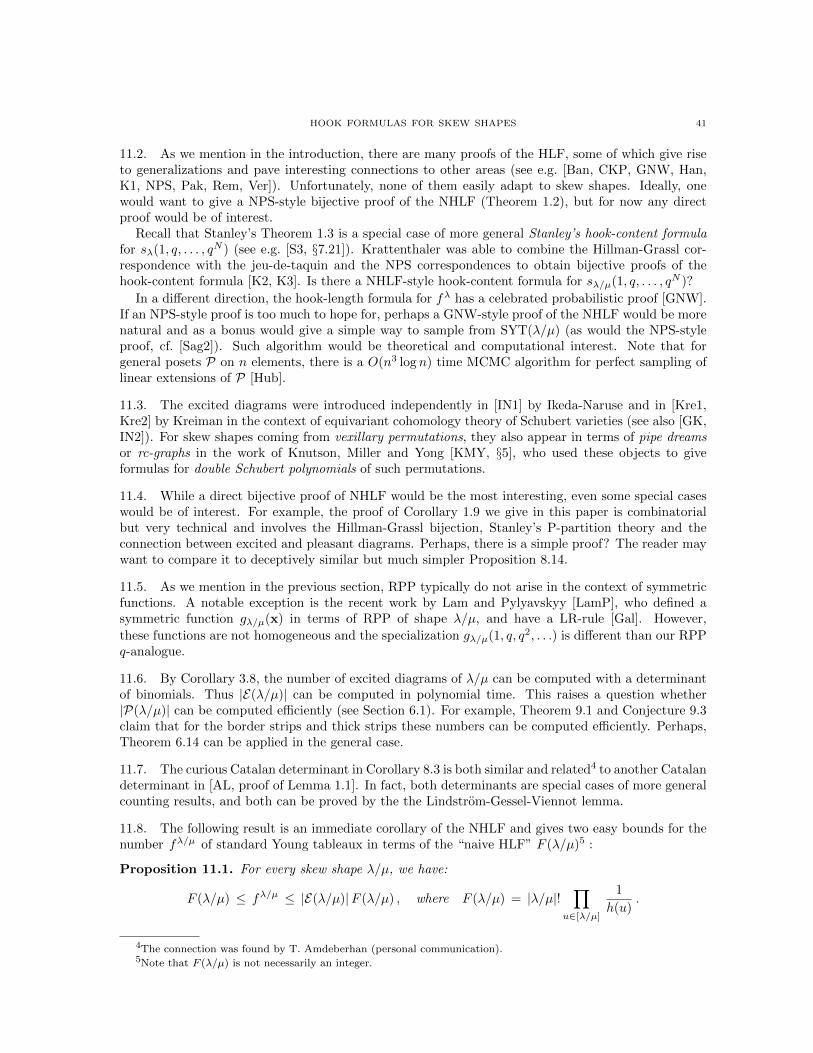
HOOK FORMULAS FOR SKEW SHAPES 41
11.2. As we mention in the introduction, there are many proofs of the HLF, some of which give riseto generalizations and pave interesting connections to other areas (see e.g. [Ban, CKP, GNW, Han,K1, NPS, Pak, Rem, Ver]). Unfortunately, none of them easily adapt to skew shapes. Ideally, onewould want to give a NPS-style bijective proof of the NHLF (Theorem 1.2), but for now any directproof would be of interest.
Recall that Stanley’s Theorem 1.3 is a special case of more general Stanley’s hook-content formulafor sλ(1, q, . . . , qN ) (see e.g. [S3, §7.21]). Krattenthaler was able to combine the Hillman-Grassl cor-respondence with the jeu-de-taquin and the NPS correspondences to obtain bijective proofs of thehook-content formula [K2, K3]. Is there a NHLF-style hook-content formula for sλ/µ(1, q, . . . , qN )?
In a different direction, the hook-length formula for fλ has a celebrated probabilistic proof [GNW].If an NPS-style proof is too much to hope for, perhaps a GNW-style proof of the NHLF would be morenatural and as a bonus would give a simple way to sample from SYT(λ/µ) (as would the NPS-styleproof, cf. [Sag2]). Such algorithm would be theoretical and computational interest. Note that forgeneral posets P on n elements, there is a O(n3 log n) time MCMC algorithm for perfect sampling oflinear extensions of P [Hub].
11.3. The excited diagrams were introduced independently in [IN1] by Ikeda-Naruse and in [Kre1,Kre2] by Kreiman in the context of equivariant cohomology theory of Schubert varieties (see also [GK,IN2]). For skew shapes coming from vexillary permutations, they also appear in terms of pipe dreamsor rc-graphs in the work of Knutson, Miller and Yong [KMY, §5], who used these objects to giveformulas for double Schubert polynomials of such permutations.
11.4. While a direct bijective proof of NHLF would be the most interesting, even some special caseswould be of interest. For example, the proof of Corollary 1.9 we give in this paper is combinatorialbut very technical and involves the Hillman-Grassl bijection, Stanley’s P-partition theory and theconnection between excited and pleasant diagrams. Perhaps, there is a simple proof? The reader maywant to compare it to deceptively similar but much simpler Proposition 8.14.
11.5. As we mention in the previous section, RPP typically do not arise in the context of symmetricfunctions. A notable exception is the recent work by Lam and Pylyavskyy [LamP], who defined asymmetric function gλ/µ(x) in terms of RPP of shape λ/µ, and have a LR-rule [Gal]. However,
these functions are not homogeneous and the specialization gλ/µ(1, q, q2, . . .) is different than our RPPq-analogue.
11.6. By Corollary 3.8, the number of excited diagrams of λ/µ can be computed with a determinantof binomials. Thus |E(λ/µ)| can be computed in polynomial time. This raises a question whether|P(λ/µ)| can be computed efficiently (see Section 6.1). For example, Theorem 9.1 and Conjecture 9.3claim that for the border strips and thick strips these numbers can be computed efficiently. Perhaps,Theorem 6.14 can be applied in the general case.
11.7. The curious Catalan determinant in Corollary 8.3 is both similar and related4 to another Catalandeterminant in [AL, proof of Lemma 1.1]. In fact, both determinants are special cases of more generalcounting results, and both can be proved by the the Lindstrom-Gessel-Viennot lemma.
11.8. The following result is an immediate corollary of the NHLF and gives two easy bounds for thenumber fλ/µ of standard Young tableaux in terms of the “naive HLF” F (λ/µ)5 :
Proposition 11.1. For every skew shape λ/µ, we have:
F (λ/µ) ≤ fλ/µ ≤ |E(λ/µ)|F (λ/µ) , where F (λ/µ) = |λ/µ|!∏
u∈[λ/µ]
1
h(u).
4The connection was found by T. Amdeberhan (personal communication).5Note that F (λ/µ) is not necessarily an integer.
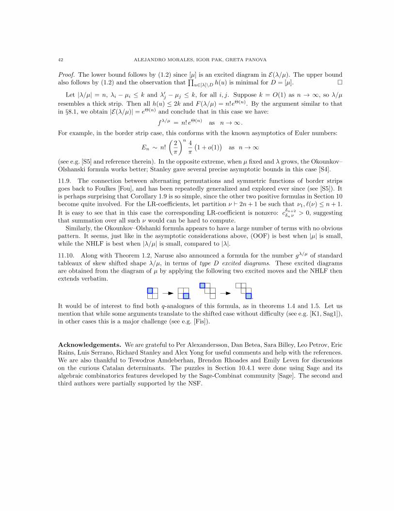
42 ALEJANDRO MORALES, IGOR PAK, GRETA PANOVA
Proof. The lower bound follows by (1.2) since [µ] is an excited diagram in E(λ/µ). The upper boundalso follows by (1.2) and the observation that
∏u∈[λ]\D h(u) is minimal for D = [µ].
Let |λ/µ| = n, λi − µi ≤ k and λ′j − µj ≤ k, for all i, j. Suppose k = O(1) as n → ∞, so λ/µ
resembles a thick strip. Then all h(u) ≤ 2k and F (λ/µ) = n!eΘ(n). By the argument similar to thatin §8.1, we obtain |E(λ/µ)| = eΘ(n) and conclude that in this case we have:
fλ/µ = n! eΘ(n) as n→∞ .
For example, in the border strip case, this conforms with the known asymptotics of Euler numbers:
En ∼ n!
(2
π
)n4
π
(1 + o(1)
)as n→∞
(see e.g. [S5] and reference therein). In the opposite extreme, when µ fixed and λ grows, the Okounkov–Olshanski formula works better; Stanley gave several precise asymptotic bounds in this case [S4].
11.9. The connection between alternating permutations and symmetric functions of border stripsgoes back to Foulkes [Fou], and has been repeatedly generalized and explored ever since (see [S5]). Itis perhaps surprising that Corollary 1.9 is so simple, since the other two positive formulas in Section 10become quite involved. For the LR-coefficients, let partition ν ` 2n+ 1 be such that ν1, `(ν) ≤ n+ 1.
It is easy to see that in this case the corresponding LR-coefficient is nonzero: cδn+2
δn ν> 0, suggesting
that summation over all such ν would can be hard to compute.Similarly, the Okounkov–Olshanki formula appears to have a large number of terms with no obvious
pattern. It seems, just like in the asymptotic considerations above, (OOF) is best when |µ| is small,while the NHLF is best when |λ/µ| is small, compared to |λ|.
11.10. Along with Theorem 1.2, Naruse also announced a formula for the number gλ/µ of standardtableaux of skew shifted shape λ/µ, in terms of type D excited diagrams. These excited diagramsare obtained from the diagram of µ by applying the following two excited moves and the NHLF thenextends verbatim.
, .
It would be of interest to find both q-analogues of this formula, as in theorems 1.4 and 1.5. Let usmention that while some arguments translate to the shifted case without difficulty (see e.g. [K1, Sag1]),in other cases this is a major challenge (see e.g. [Fis]).
Acknowledgements. We are grateful to Per Alexandersson, Dan Betea, Sara Billey, Leo Petrov, EricRains, Luis Serrano, Richard Stanley and Alex Yong for useful comments and help with the references.We are also thankful to Tewodros Amdeberhan, Brendon Rhoades and Emily Leven for discussionson the curious Catalan determinants. The puzzles in Section 10.4.1 were done using Sage and itsalgebraic combinatorics features developed by the Sage-Combinat community [Sage]. The second andthird authors were partially supported by the NSF.
HOOK FORMULAS FOR SKEW SHAPES 43
References
[AR] R. Adin and Y. Roichman, Standard Young tableaux, in Handbook of Enumerative Combinatorics (M. Bona,
editor), CRC Press, Boca Raton, 2015, 895–974.[AL] T. Amdeberhan and E. Leven, Multi-cores, posets, and lattice paths, Adv. Appl. Math. 71 (2015), 1–13.
[AJS] H.H. Andersen, J.C. Jantzen and W. Soergel, Representations of quantum groups at p-th root of unity and of
semisimple groups in characteristic p: independence of p, Asterisque, 220, 321.[Ban] J. Bandlow, An elementary proof of the hook formula, Electron. J. Combin. 15 (2008), RP 45, 14 pp.
[BR] Y. Baryshnikov and D. Romik, Enumeration formulas for Young tableaux in a diagonal strip, Israel J. Math.
178 (2010), 157–186.[Bil] S. Billey, Kostant polynomials and the cohomology ring for G/B, Duke Math. J. 96 (1999), 205–224.
[BGR] A. Borodin, V. Gorin and E. M. Rains, q-distributions on boxed plane partitions, Selecta Math. 16 (2010),
731–789.[CYY] W. Y. C. Chen, A. L. B. Yan and G.-G. Yang, Transformations of border strips and Schur function determinants,
J. Algebraic Combin. 21 (2005), 379–394.
[CS] X. Chen and R. P. Stanley, A formula for the specialization of skew Schur functions, to appear in Ann. Comb.;available at www-math.mit.edu/∼rstan/papers/q-oo.pdf.
[CKP] I. Ciocan-Fontanine, M. Konvalinka and I. Pak, The weighted hook length formula, J. Combin. Theory, Ser. A.118 (2011), 1703–1717.
[SV] M. de Sainte-Catherine and X. G. Viennot, Enumeration of certain Young tableaux with bounded height, in
Lecture Notes Math. 1234, Springer, Berlin, 1986, 58–67.[Deu] E. Deutsch, An involution on Dyck paths and its consequences, Discrete Math. 204 (1999), 163–166.
[Fis] I. Fischer, A bijective proof of the hook-length formula for shifted standard tableaux, arXiv:math/0112261.
[Fou] H. O. Foulkes, Tangent and secant numbers and representations of symmetric groups, Discrete Math. 15 (1976),311–324.
[FRT] J. S. Frame, G. de B. Robinson and R. M. Thrall, The hook graphs of the symmetric group, Canad. J. Math. 6
(1954), 316–324.[Gal] P. Galashin, A Littlewood-Richardson rule for dual stable Grothendieck polynomials, arXiv:1501.00051.
[G1] E. R. Gansner, The Hillman-Grassl correspondence and the enumeration of reverse plane partitions, J. Combin.
Theory, Ser. A 30 (1981), 71–89.[G2] E. R. Gansner, Matrix correspondences of plane partitions, Pacific J. Math. 92 (1981), 295–315.
[GV] I. M. Gessel and X. G. Viennot, Determinants, paths and plane partitions, preprint (1989); available attinyurl.com/zv3wvyh.
[GJ] I. P. Goulden and D. M. Jackson, Combinatorial enumeration, John Wiley, New York, 1983.
[GK] W. Graham and V. Kreiman, Excited Young diagrams, equivariant K-theory, and Schubert varieties, Trans.AMS 367 (2015), 6597–6645.
[GNW] C. Greene, A. Nijenhuis and H. S. Wilf, A probabilistic proof of a formula for the number of Young tableaux
of a given shape, Adv. Math. 31 (1979), 104–109.[HaG] A. M. Hamel and I. P. Goulden, Planar decompositions of tableaux and Schur function determinants, European
J. Combin. 16 (1995), 461–477.
[Han] G.-N. Han, The Nekrasov-Okounkov hook length formula: refinement, elementary proof, extension and appli-cations, Ann. Inst. Fourier 60 (2010), 1–29.
[HiG] A. P. Hillman and R. M. Grassl, Reverse plane partitions and tableau hook numbers, J. Combin. Theory,
Ser. A 21 (1976), 216–221.[Hub] M. Huber, Fast perfect sampling from linear extensions, Discrete Math. 306 (2006), 420–428.
[IN1] T. Ikeda and H. Naruse, Excited Young diagrams and equivariant Schubert calculus, Trans. AMS 361 (2009),5193–5221.
[IN2] T. Ikeda and H. Naruse, K-theoretic analogues of factorial Schur P- and Q-functions, Adv. in Math. 243 (2012),22–66.
[Jon] J. Jonsson, Generalized triangulations and diagonal-free subsets of stack polyominoes, J. Combin. Theory,
Ser. A 112 (2005), 117–142.
[KK] B. Kostant and S. Kumar, The nil Hecke ring and cohomology of G/P for Kac-Moody group, Adv. in Math. 62(1986) 183–237.
[Knu] A. Knutson, A Schubert calculus recurrence from the noncomplex W -action on G/B, arXiv:0306304.[KMY] A. Knutson, E. Miller and A. Yong, Grobner geometry of vertex decompositions and of flagged tableaux,
J. Reine Angew. Math. 630 (2009), 1–31.
[KT] A. Knutson and T. Tao, Puzzles and (equivariant) cohomology of Grassmannians, Duke Math J. 119 (2003),
221–260.[K1] C. Krattenthaler, Bijective proofs of the hook formulas for the number of standard Young tableaux, ordinary
and shifted, Electron. J. Combin. 2 (1995), RP 13, 9 pp.[K2] C. Krattenthaler, An involution principle-free bijective proof of Stanley’s hook-content formula, Discrete Math.
Theor. Comput. Sci. 3 (1998), 11–32.
44 ALEJANDRO MORALES, IGOR PAK, GRETA PANOVA
[K3] C. Krattenthaler, Another involution principle-free bijective proof of Stanley’s hook-content formula, J. Combin.
Theory, Ser. A 88 (1999), 66–92.[K4] C. Krattenthaler, Plane partitions in the work of Richard Stanley and his school, arXiv:1503.05934.
[Kre1] V. Kreiman, Schubert classes in the equivariant K-theory and equivariant cohomology of the Grassmannian,
arXiv:math.AG/0512204.[Kre2] V. Kreiman, Schubert classes in the equivariant K-theory and equivariant cohomology of the Lagrangian Grass-
mannian, arXiv:math.AG/0602245.[LamP] T. Lam and P. Pylyavskyy, Combinatorial Hopf algebras and K-homology of Grassmannians, IMRN 2007
(2007), No. 24, 1–48.
[LasP] A. Lascoux and P. Pragacz, Ribbon Schur functions, European J. Combin. 9 (1988), 561–574.[LS] A. Lascoux and M.-P. Schutzenberger, Polynomes de Schubert (in French), C.R. Acad. Sci. Paris Ser. I
Math. 294 (1982), 447–450.
[MPP] A.H. Morales, I. Pak and G. Panova, Multivariate hook formulas from Schubert calculus, in preparation.[MS] A. I. Molev and B. E. Sagan, A Littlewood-Richardson rule for factorial Schur functions, Trans. AMS 351
(1999), 4429–4443.
[Nara] H. Narayanan, On the complexity of computing Kostka numbers and Littlewood-Richardson coefficients, J.Algebr. Comb. 24 (2006), 347–354.
[Naru] H. Naruse, Schubert calculus and hook formula, talk slides at 73rd Sem. Lothar. Combin., Strobl, Austria,
2014; available at tinyurl.com/z6paqzu.[NPS] J.-C. Novelli, I. Pak and A. V. Stoyanovskii, A direct bijective proof of the hook-length formula, Discrete Math.
Theor. Comput. Sci. 1 (1997), 53–67.[OO] A. Okounkov and G. Olshanski, Shifted Schur functions, St. Petersburg Math. J. 9 (1998), 239–300.
[Pak] I. Pak, Hook length formula and geometric combinatorics. Sem. Lothar. Combin. 46 (2001), Art. B46f, 13 pp.
[Rem] J. B. Remmel, Bijective proofs of formulae for the number of standard Young tableaux, Linear and MultilinearAlgebra 11 (1982), 45–100.
[Sag1] B. E. Sagan, Enumeration of partitions with hooklengths, European J. Combin. 3 (1982), 85–94.
[Sag2] B. E. Sagan, The Symmetric Group, Springer, 2000.[Sag3] B. E. Sagan, Probabilistic proofs of hook length formulas involving trees, Sem. Lothar. Combin. 61A (2009),
Art. B61Ab, 10 pp.
[Sage] The Sage-Combinat community. Sage-Combinat: enhancing Sage as a toolbox for computer exploration inalgebraic combinatorics, 2013. http://combinat.sagemath.org.
[SS] L. Serrano and C. Stump, Maximal fillings of moon polyominoes, simplicial complexes, and Schubert polyno-
mials, Electron. J. Combin. 19 (2012), RP 16, 18 pp.[OEIS] N. J. A. Sloane, The Online Encyclopedia of Integer Sequences, oeis.org.
[S1] R. P. Stanley, Theory and applications of plane partitions, Part 2, Stud. Appl. Math. 50 (1971), 259–279.
[S2] R. P. Stanley, The conjugate trace and trace of a plane partition, J. Combin. Theory, Ser. A 14 (1973), 53–65.[S3] R. P. Stanley, Enumerative Combinatorics, vol. 1 (second ed.) and vol. 2 (first ed.), Cambridge Univ. Press,
2012 and 1999.[S4] R. P. Stanley, On the enumeration of skew Young tableaux, Adv. Appl. Math. 30 (2003), 283–294.
[S5] R. P. Stanley, A survey of alternating permutations, in Combinatorics and graphs, AMS, Providence, RI, 2010,
165–196.[S6] R. P. Stanley, Catalan Numbers, Cambridge Univ. Press, 2015.
[Ste] J. R. Stembridge, On the fully commutative elements of Coxeter groups, J. Algebraic Combin. 5 (1996), 353–
385.[Sul] R. A. Sulanke, The Narayana distribution, J. Statist. Plann. Inference 101 (2002), 311–326.[TY] H. Thomas and A. Yong, Equivariant Schubert calculus and jeu de taquin, to appear in Ann. Inst. Fourier;
arXiv:1207.3209.[Tym] J. S. Tymoczko, Billey’s formula in combinatorics, geometry, and topology; arXiv:1309.0254.
[Vie] G. Viennot, Une forme geometrique de la correspondance de Robinson-Schensted, in Lecture Notes Math. 579,
Springer, Berlin, 1977, 29–58.[Ver] A. M. Vershik, The hook formula and related identities, J. Soviet Math. 59 (1992), 1029–1040.[Wac] M. Wachs, Flagged Schur functions, Schubert polynomials, and symmetrizing operators, J. Combin. Theory,
Ser. A 40 (1985), 276–289.[Whi] D. E. White, Some connections between the Littlewood–Richardson rule and the construction of Schensted,
J. Combin. Theory, Ser. A 30 (1981), 237–247.