Embed Size (px)
DESCRIPTION
Georgia Skew
Citation preview

7/21/2019 Georgia Skew
http://slidepdf.com/reader/full/georgia-skew 1/182
March 14, 1975
A NOTE TO USERS WHO ARE
NOT IN THE GEORGIA DOT ...
This is a reprint of the User's Manual as prepared in 1968. It remains technically
up to date.
However, there was a reorganization of Georgia State Government in July,1972. Therefore, all queries concerning this manual or the program should
be addressed to
OFFICE OF SYSTEMS DEVELOPMENT
GEORGIA DEPARTMENT OF TRANSPORTATION
NO. 2 CAPITOL SQUARE
ATLANTA, GA 30334
7/21/2019 Georgia Skew
http://slidepdf.com/reader/full/georgia-skew 2/182
FOREWORD
During the past decade the electronic computer has played an ever increasing role in
Highway Engineering, especially in the field of Bridge Design. The great motivation for
this role was the National Interstate Highway Act passed in
1956. The impact of this new system of super highways with their complex interchanges
created the need for a new approach in the design and construction of highways. The high-
speed electronic computer has proved to be the answer, particularly in the solution ofbridge geometry.
Before the computer age, the geometry of a bridge was a major factor used to
determine the location and type of structure. The voluminous amount of computations
required for the geometric solution of curved bridges in transition often made it more
feasible to use an otherwise uneconomical straight bridge. Usually the time required for
the geometric computations proved to be greater than the time required for design. Today,
the computer has assumed the geometric burden-and much of the design also-and thereby
freed the Engineer from these time-consuming tasks. The Bridge Engineer, using the
computer as a design aid, can devote more of his time to the economics and esthetics of
design. This time saving-including other areas of Highway Engineering-not only has
resulted in more economical structures but, in a larger sense, it will make possible thecompletion of the Interstate and other highway systems at an earlier date.
"The Geometric Solution of Highway Bridges" presented in this report is a problem
oriented computer program that can solve nearly all the geometric requirements for the
design, detailing, and construction of highway bridges. This program is actually the third
in a series of bridge geometry programs. The first geometry program was written in 1957
for an IBM 650 computer using machine language. This program proved so successful that an
effort was made immediately to apply data processing to other areas of Bridge Engineering.
The second geometry program, written in 1963, was a complete revision of the first program;
however, many improvements were incorporated into the new program. The IBM 1620 computer
was being used at that time, so the computer oriented Symbolic Programming System language
(SPS) was used. Now the program has been rewritten in Fortran IV programming language.Again, the program has been made more versatile with revisions and additional features. It
is significant to note the evolution of the programming language with each succeeding
computer generation. This, however, is not the ultimate geometry program. Although the
pace at which data processing has been applied to Highway Engineering has exceeded the
expectations of a decade ago, the surface appears only to have been scratched.
"The Geometric Solution of Highway Bridges" computer program is more commonly
referred to as the "Skewed Bridge" program, primarily for the sake of brevity. In fact,
this is the name that is shown on the input data form and in the output data of the
program.
This write-up is primarily a user's manual and does not include flow charts,
a program listing, nor a comprehensive report on the method of solution. However, the
method of solution is discussed in general terms so that the user will be able to get a
general idea of the method of solution used by the program. Since a source deck can be
obtained by request, a program listing can be obtained by listing or compiling the source
deck. Also, since the program is written in Fortran IV programming language, and contains
numerous comment cards that describe the program functions, the flow charts are not really
essential in order to understand the procedure of the program solution.

7/21/2019 Georgia Skew
http://slidepdf.com/reader/full/georgia-skew 3/182
The reader is assumed to be familiar with the standard terminology of Highway
Engineering, and such terms as Station, Superelevation, Transition, Survey line, Degree-
of-Curvature, etc., will not be defined in this report. It should be noted that the term
"Mainline" as used in this report is synonymous with the survey line, and the term "Bent"
is used to designate a substructure unit, i.e., pier, abutment, etc.
This report, then., explains in detail the functions of the program and how theprogram can be effectively applied in order to solve the geometric requirements of a
highway bridge.
Glenn H. Sikes
Atlanta., Georgia
September 16, 1968
7/21/2019 Georgia Skew
http://slidepdf.com/reader/full/georgia-skew 4/182
ACKNOWLEDGMENT
The programming of "The Geometric Solution of Highway Bridges" computer program was
undertaken by the direction and under the authority of Mr. Russell L. Chapman, Jr., StateHighway Bridge Engineer. Mr. Chapman is a pioneer in the field of application of
electronic computation to problems related to the design and construction of bridges and
assisted in developing the method of solution used by the original "Skewed Bridge"
computer program. His encouragement and support has been a vital factor in the application
of data processing to Bridge Engineering.
A special acknowledgment is due Mr. Jose M. Nieves-Olmo, formerly Assistant Highway
Bridge Engineer with The State Highway Department of Georgia, who developed the method of
solution and wrote the IBM 650 and IBM 1620 versions of the "Skewed Bridge" computer
program. His accomplishments in the field of data processing has been-and continues to be-
of immeasurable benefit to The State Highway Department of Georgia and many other States
as well.
Mr. Thomas S. Moss, Jr., developed and wrote a considerable part of the program
presented in this write-up before leaving the employment of The State Highway Department.
His excellent work was very beneficial in the final completion of this work.
Many employees of The State Highway Department of Georgia assisted in the preparation
of this manual. Their criticisms, suggestions, and assistance in drawing the figures has
made possible the editing of this program write-up. And a special acknowledgment and
"Thanks" go to Mrs. Faye Bates who had the task of typing the entire manuscript.

7/21/2019 Georgia Skew
http://slidepdf.com/reader/full/georgia-skew 5/182
DISCLAIMER
Although this program has been subjected to many rigorous tests - all with excellent
results - no warranty, expressed or implied, is made by The State Highway Department of
Georgia as to the accuracy and functioning of the program,, nor shall the fact of
distribution constitute any such warranty, and no responsibility is assumed by The State
Highway Department of Georgia in any connection therewith.
7/21/2019 Georgia Skew
http://slidepdf.com/reader/full/georgia-skew 6/182
THIS VOLUME., OR ANY PART THEREOF, MUST
NOT BE REPRODUCED IN ANY FORM NOR
DISTRIBUTED TO ANY OTHER ORGANIZATION
WITHOUT THE WRITTEN PERMISSION OF
THE STATE HIGHWAY DEPARTMENT OF GEORGIA.
7/21/2019 Georgia Skew
http://slidepdf.com/reader/full/georgia-skew 7/182
TABLE OF CONTENTS
PAGE
I. PROGRAM ABSTRACT 1
II. DESCRIPTION OF PROGRAM 2
III. PREPARING THE INPUT DATA 12
LAYOUT DATA 14
LONGITUDINAL LINES 50
SPAN DATA 80
IV. THE OUTPUT DATA 116
V. ERROR MESSAGES 124
VI. EXAMPLE PROBLEMS 128
VII. OPERATING PROCEDURE 183COMPATIBILITY 183
COMPILING THE PROGRAM 184
KEY-PUNCH INSTRUCTIONS 185
COMPUTER OPERATOR INSTRUCTIONS 186
VIII. BLANK INPUT DATA FORMS 188
LAYOUT DATA 188
LONGITUDINAL LINE 189
SPAN DATA 190
COORDINATE TYPE DATA 191
7/21/2019 Georgia Skew
http://slidepdf.com/reader/full/georgia-skew 8/182
I. PROGRAM ABSTRACT
TITLE: THE GEOMETRIC SOLUTION OF HIGHWAY BRIDGES
AUTHOR: Glenn H. Sikes
Highway Bridge Engineer
PURPOSE/DESCRIPTION: The purpose of this program is to solve the geometries that arerequired in the design, detailing and construction of highway bridges and, thereby,
relieve the Engineer of this time-consuming task and, in addition, remove the geometric
limitations in the design of bridge structures. The program solves the geometries by
intersecting a series of longitudinal lines, that run basically parallel to the bridge,
with a series of transverse lines that lie basically across the bridge. The computed da
(including the finished grade elevation) at each intersection point is reported as the
output data. The longitudinal lines may be composed of beams, gutters, curbs, railings,
etc., whereas the transverse lines can be bents, centerline bearings, diaphragms,
construction joints, splice points, etc. The input data is entered on forms provided fo
the Engineer.
METHOD OF SOLUTION: The bridge is oriented on a user-defined coordinate system of X andaxes. The longitudinal and transverse lines are set up in equation form and intersected
computing the solutions of simultaneous equations. The data given in the output at the
intersection points of the longitudinal and transverse lines is computed using the basi
concepts of analytic geometry.
RESTRICTIONS/RANGE: The bridge may be located in one, two or three combinations of
horizontal curves and tangents. The horizontal curves may be compound but not reverse
curves (work as two problems). The survey line cannot be a spiral for the purpose of
computing stations. Vertical alignment is limited to two vertical curves with
corresponding tangents. The surface of the bridge may be level, superelevated (with one
six lanes in constant or transition superelevation), or parabolic. The maximum number o
longitudinal lines is thirty, and the maximum number of T-Lines is twenty per span withlimitation on the number of spans.
PROGRAMMING LANGUAGE: The program is written in Basic Fortran IV programming language
primarily to obtain computer independency. The long form of floating-point data
representation is used for all arithmetical computations, thereby insuring sufficient
accuracy.
ADDITIONAL REMARKS: Core Storage requirements are approximately 58,000 positions (bytes)
The processing time will vary depending on the amount of input data, with the average
problem requiring approximately one and one-half minutes (IBM 36o, Mod. 30). All input is
from punched cards, and the output is listed by the printer. No other intermediate I/
devices are used.
DIRECT INQUIRIES TO: Russell L. Chapman, Jr.
State Highway Bridge Engineer
State Highway Department of Georgia
#2 Capitol Square
Atlanta, Georgia 30334
Telephone No. 688-5201, Ext. 371
7/21/2019 Georgia Skew
http://slidepdf.com/reader/full/georgia-skew 9/182
II. DESCRIPTION OF PROGRAM
"The Geometric Solution of Highway Bridges" is a problem oriented computer program
that can be used effectively to compute the geometric requirements for the design,
detailing and construction of highway bridges. Actually, the program is not limited to
highway bridges since the geometry of railroad and pedestrian bridges is easily solved by
this program. The geometric solution of a problem fundamentally consists of intersecting
a series of longitudinal lines that run basically parallel to the bridge, with a series of
transverse lines that run basically across the bridge. Actually, the transverse lines may
be series of points (centerline of bearings, etc.) located on the longitudinal lines
(beams, etc.) and do not necessarily have to lie on a straight line. At the intersections
of the longitudinal and transverse lines, the program computes the following types of
data.
Stations
The station of each intersection point computed by the program is given in the
output data. In addition to the station, the output data will contain the radial or
perpendicular distance from the point to the survey line. This distance, together with the
station, completely locates each intersection point for the Engineer.
Elevations
The elevations computed by the program at the intersection points are finished grade
elevations, i.e., top of bridge surface elevation at the intersection points. These
elevations which are essential in all phases of Bridge Engineering form an important part
of the output data of each problem.
Distances and Lengths
The distances or lengths between intersection points measured along the longitudinal
and transverse lines are computed by the program and listed in the output. This
information is of considerable benefit in the detailing process.
Angles
The angles between the longitudinal and transverse lines, or skew angles, are
computed by the program and listed in the output data. These angles can also be of
considerable benefit when detailing the bridge.
Coordinates
The X and Y Coordinates of each point of intersection are computed by the program in
the solution of the longitudinal and transverse line equations in order to compute the
aforementioned data. These coordinates are the result of the orientation of the bridge on
a system of coordinate axes in order to facilitate the solution of the problem.
BRIDGE LAYOUT
In order to solve the geometric requirements, the bridge must be placed on a
coordinate system of X and Y axes. After the Engineer has defined the orientation of
bridge in the input data, the longitudinal and transverse lines can be set up in equati
form by the program, and the solution of the problem then becomes basically one of solv
simultaneous equations.
7/21/2019 Georgia Skew
http://slidepdf.com/reader/full/georgia-skew 10/182
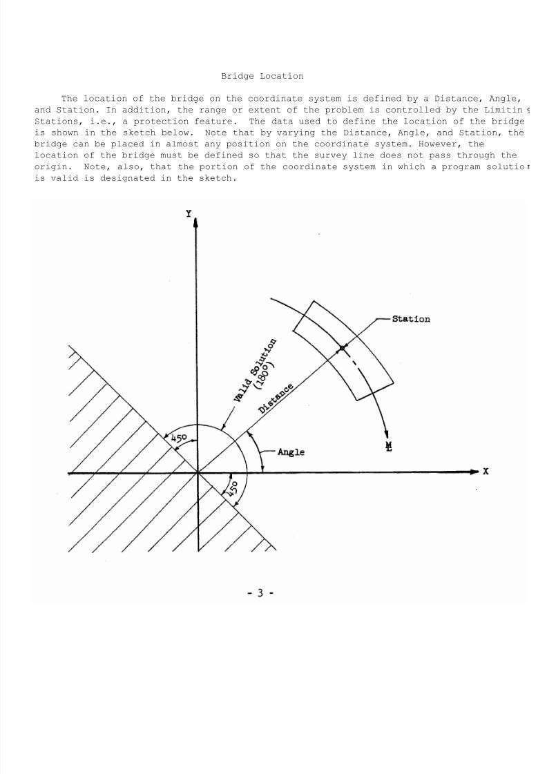
Bridge Location
The location of the bridge on the coordinate system is defined by a Distance, Angl
and Station. In addition, the range or extent of the problem is controlled by the Limit
Stations, i.e., a protection feature. The data used to define the location of the bri
is shown in the sketch below. Note that by varying the Distance, Angle, and Station, bridge can be placed in almost any position on the coordinate system. However, the
location of the bridge must be defined so that the survey line does not pass through th
origin. Note, also, that the portion of the coordinate system in which a program solu
is valid is designated in the sketch.
7/21/2019 Georgia Skew
http://slidepdf.com/reader/full/georgia-skew 11/182
Horizontal Alignment
The horizontal alignment is defined by giving the degree-of-curvature of each range
of horizontal curve, and the P.C. and P.T. Stations that separate the range of the curves.
The program has the capacity for three ranges of horizontal curves and tangents.
Following is a list of the possible combinations of tangents and circular curves that may
be used to define the horizontal alignment.
One Range:
1. Tangent
2. Curve
Two Ranges:
1. Tangent-Curve
2. Curve-Tangent
3. Curve-Curve (compound curve)
Three Ranges:
1. Tangent-Curve-Curve
2. Curve-Tangent-Curve
3. Curve-Curve-Tangent
4. Tangent - Curve - Tangent
5. Curve-Curve-Curve
A tangent is defined as a curve with a degree-of-curvature equal to zero.
The horizontal alignment defines the line that the stations are measured along,commonly called the survey line or mainline. Only one survey line can be defined with
each problem, and that survey line must be a tangent (straight), circular curve, or a
combination as shown above. The program has no provision for a spiral survey line,
although the longitudinal lines may be defined as spirals (curve taper). The horizontal
alignment may be composed of compound curves; however, the program has no provision for
reverse curves. This presents no problem, however, since a bridge on a reverse curve can
be solved by dividing the bridge at the point of reverse curvature into two problems.
The program solves a problem with a curve mainline regardless whether the mainline is
curving to the left or right. Actually, the solution of the problem is independent of the
direction of the curve since a left curve is a mirror image of a right curve, and vice
versa. In the sketch on the following page, a right curve is shown at the top and a left
curve is shown at the bottom. Note that the direction of the plus and minus Y-axis has
been reversed in the sketch of the left curve; and, in addition, the positions of the
normally first and fourth quadrant have been interchanged. If the sketch is rotated about
the X-axis and viewed from the back, the left and right curves will appear to have
reversed their direction. In other words, when a right curve is viewed from underneath it
appears as a left curve. Therefore., since the direction from which a bridge is viewed
no physical effect on the alignment, the solution of the problem should be-and is-
completely independent of the direction of the curve.
7/21/2019 Georgia Skew
http://slidepdf.com/reader/full/georgia-skew 12/182
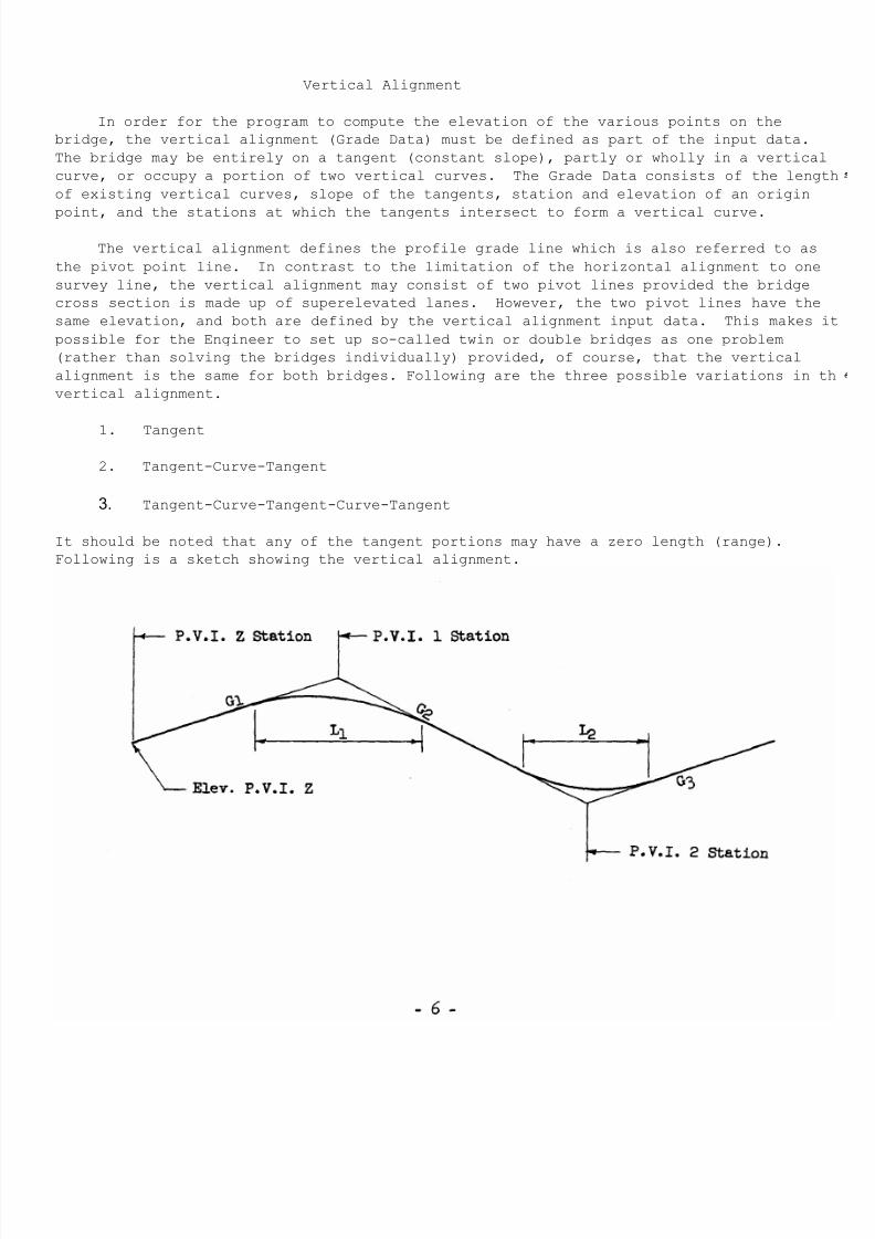
Vertical Alignment
In order for the program to compute the elevation of the various points on the
bridge, the vertical alignment (Grade Data) must be defined as part of the input data.
The bridge may be entirely on a tangent (constant slope), partly or wholly in a vertica
curve, or occupy a portion of two vertical curves. The Grade Data consists of the len
of existing vertical curves, slope of the tangents, station and elevation of an origin
point, and the stations at which the tangents intersect to form a vertical curve.
The vertical alignment defines the profile grade line which is also referred to as
the pivot point line. In contrast to the limitation of the horizontal alignment to on
survey line, the vertical alignment may consist of two pivot lines provided the bridge
cross section is made up of superelevated lanes. However, the two pivot lines have th
same elevation, and both are defined by the vertical alignment input data. This makes
possible for the Engineer to set up so-called twin or double bridges as one problem
(rather than solving the bridges individually) provided, of course, that the vertical
alignment is the same for both bridges. Following are the three possible variations in
vertical alignment.
1. Tangent
2. Tangent-Curve-Tangent
3. Tangent-Curve-Tangent-Curve-Tangent
It should be noted that any of the tangent portions may have a zero length (range).
Following is a sketch showing the vertical alignment.
7/21/2019 Georgia Skew
http://slidepdf.com/reader/full/georgia-skew 13/182
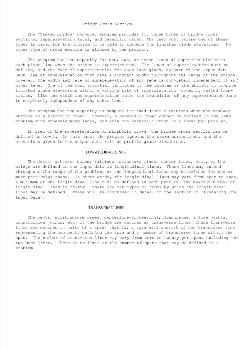
Bridge Cross Section
The "Skewed Bridge" computer program provides for three types of bridge cross
sections: superelevation level, and parabolic crown. The user must define one of these
types in order for the program to be able to compute the finished grade elevations. N
other type of cross section is allowed by the program.
The program has the capacity for one, two, or three lanes of superelevation witheach pivot line when the bridge is superelevated. The lanes of superelevation must be
defined, and the rate of superelevation for each lane given, as part of the input data
Each lane of superelevation must have a constant width throughout the range of the brid
however, the width and rate of superelevation of any lane is completely independent of
other lane. One of the most important functions of the program is the ability to comp
finished grade elevations within a varying rate of superelevation, commonly called tran
sition. Like the width and superelevation rate, the transition of any superelevated l
is completely independent of any other lane.
The program has the capacity to compute finished grade elevations when the roadway
surface is a parabolic crown. However, a parabolic crown cannot be defined in the sam
problem with superelevated lanes, and only one parabolic crown is allowed per problem.
In lieu of the superelevation or parabolic crown, the bridge cross section can be
defined as level. In this case, the program ignores the crown corrections, and the
elevations given in the output data will be profile grade elevations.
LONGITUDINAL LINES
The beams, gutters, curbs, railings, structure lines, center lines, etc., of the
bridge are defined in the input data as longitudinal lines. These lines may extend
throughout the range of the problem, or the longitudinal lines may be defined for one o
more particular spans. In other words, the longitudinal lines may vary from span to s
A minimum of one longitudinal line must be defined in each problem. The maximum number longitudinal lines is thirty. There are ten types or codes by which the longitudinal
lines may be defined. These will be discussed in detail in the section on "Preparing
Input Data".
TRANSVERSE LINES
The bents, substructure lines, centerline-of-bearings, diaphragms, splice points,
construction joints, etc. of the bridge are defined as transverse lines. These transver
lines are defined in units of a span; that is, a span will consist of two transverse li
representing the two bents defining the span and a number of transverse lines within th
span. The number of transverse lines may vary from zero to twenty per span, excluding
two bent lines. There is no limit on the number of spans that may be defined in aproblem.
7/21/2019 Georgia Skew
http://slidepdf.com/reader/full/georgia-skew 14/182
USING THE PROGRAM
The Engineer can effectively use the "Skewed Bridge" computer program in the
preliminary and final design of a bridge. In the preliminary phase, stations, skew
angles, distances, etc., that are unknown can be computed by the program to assist in t
preliminary layout. In the final design phase, the lengths of beams and diaphragms,
position of diaphragms, elevations for determining beam seat elevations and many other
types of pertinent data can be computed by this program, thereby assisting the Engineerthe design and detailing of the bridge. In the construction phase, the Engineer can
easily use the program to obtain the elevations used to set the construction forms, etc
It is important to note that any bridge may be set up as a number of separate
problems and processed at different times. For example, the geometric requirements in
design stage are quite different from the geometry that an Engineer requires in the
construction of the same bridge. However, it is usually more beneficial to have all t
geometric requirements in the design process computed in a single run of the problem.
Later, the Construction Engineer can compute his geometric requirements in another run
the problem.
The information required by the program in order to process the problem must begiven by the Engineer on a set of input data forms. First, it is important to determi
all the different types of information the user desires the program to compute. This
eliminate the possibility of having to run the problem again to compute data not includ
in the first run of the problem. Next, the input data required by the program to comp
the desired output must be determined. This involves choosing the number and types of
longitudinal and transverse lines, etc. Finally, this data must be entered on the input
data forms and forwarded to the Data Processing Center.
The output data which contains a listing of the input data is fully edited with
numerous headings for ease in interpretation. The accuracy of the output data depends
directly on the accuracy of the input data. That is, if an error is made in the input
data, it surely will result in erroneous answers appearing in the output data. It canbe overemphasized that the entire input data should be thoroughly checked before
processing, and it is suggested that the input data forms be compared to the listing of
the input data that is given in the output data as a further check.
7/21/2019 Georgia Skew
http://slidepdf.com/reader/full/georgia-skew 15/182
METHOD OF SOLUTION
The geometric solution of a problem is based on the concepts of analytic geometry,
i.e., coordinate system, line equations, etc. The program solution has three basic
functions and following is a discussion of each function.
1. Compute Line Equations.
The mainline, longitudinal lines and transverse lines are set up in equation
form by the program. Three basic types of line equations are used to describe these
lines: straight, circular curve and spiral.
Straight Lines
The equation of a straight line is set up in slope intercept form:
Y = M*X + B
Where "M" is the slope of the line and "B" is the Y-Coordinate of the point where
the line crosses the Y-axis.
However, if the absolute value of the slope (M) is greater than one (1), the
equation of the straight line is in the following form:
X = N*Y + C
Where "N" is the slope of the line in relation to the Y-axis (N = l/M), and "C" is
the X-Coordinate of the point where the line intersects the X-axis (C = -B/M).
Circular Curve Lines
The equation of a circle is set up in the following form:
(X-X0)2
+ (Y-Y0)2
= R2
Where "X0" and "Y0" are the coordinates of the center of the circle, and "R" is the
radius of the circle.
Spiral lines
The equation of a spiral (curve taper) is set up in polar coordinate form as
follows:
R =KΘ
Where "R" is the radius of the curve when a radial line is rotated an angle equal to
"Θ", and "K" is a constant representing the change in radius per unit of angle
rotation.
7/21/2019 Georgia Skew
http://slidepdf.com/reader/full/georgia-skew 16/182
2. Intersect Lines.
The program intersects each longitudinal line with the transverse lines. In
addition, the mainline is intersected with all bent lines. The equations are solved
simultaneously and, thereby, the X and Y coordinates are determined. When solving
for the intersection of a spiral and straight line, the program uses a process of
“approximations”.
3. Compute Intersection Data.
After solving for the X and Y coordinates, the program computes the station of
the point and the distance from the point to the mainline. Using this data, the
elevation of the point can be computed. In addition, other distances and angles are
computed and printed in the output data.
Solution Sequence
Following is a brief outline of the sequence of the program solution with comments to
indicate the functions of each part of the program solution.
1. Read and Process Layout Data (one time per problem).
a. Location Data.
The coordinates of the Reference Point Station are computed and stored
along with the Limiting Stations, Reference Angle and Reference Point Station.
b. Horizontal Data.
The equation of the mainline, P.C. and P.T. Station coordinates, and
Reference Angles are computed and stored along with the degree-of-curvature and
radius of each range of horizontal curve.
C. Vertical Curve Data.
The vertical curve alignment is divided into ranges of parabolic curves
and tangents, and the equation of the profile grade line is computed for each
range and stored for future reference.
d. Crown and lane Definitions.
If the roadway is a parabolic crown, the program computes the
parabolic constant and stores this constant along with the limits
and position of the parabolic crown. When the bridge surface is
superelevated, the program computes the width of each lane and stores
this data along with the position of the lanes and profile grade
lines.
e. Superelevation Data.
If the bridge surface is superelevated, the rate of superelevation of each
lane is read and stored. If the bridge is in a varying rate of transition, the
rates of change of the superelevation rates are computed for each lane and
stored along with the stations of the breaks in the transition rates. This
enables the program to compute the rate of superelevation in any lane at any
station.

7/21/2019 Georgia Skew
http://slidepdf.com/reader/full/georgia-skew 17/182
2. Read and Process Longitudinal Lines.
The program reads the longitudinal line data and computes and stores the
equation of each longitudinal line that does not vary within the range of the
problem. This is repeated each time a set of longitudinal lines is defined in the
input data.
3. Read and Process Span.
The following program steps are repeated for each span in the bridge.
a. Span Identification.
The program reads and prints the information used to describe the span,
i.e., remarks, etc.
b. Bent Data.
The input data of each bent is read and printed. Then, the programcomputes the equation of each bent and intersects the two bents with the
mainline in order to find the bent station and skew angle (if this data is not
given in the input data). The bent station and skew angle are stored for
future listing.
4. Intersect Bents with Longitudinal Lines.
The program solves for the intersection of each bent with each longitudinal
line. The intersection data (coordinates, angles, stations, etc.) is stored for
future reference and listing. In addition, the equations of the variable
longitudinal lines are computed, i.e., chords, etc.
5. Read and Process Transverse Lines in Span.
The program reads and prints the input data of each transverse line in the
span. At the same time, the equations of the transverse lines are computed. These
equations are stored temporarily so that these lines can be intersected with the
longitudinal lines.
6. Intersect Longitudinal and Transverse Lines.
Beginning with the first longitudinal line, the program intersects the
longitudinal lines with each transverse line. After each intersection point is
found, the program computes the various output data (station, elevation, distances,
angles). After processing all longitudinal lines, the program proceeds to a new span
or terminates operation.
7/21/2019 Georgia Skew
http://slidepdf.com/reader/full/georgia-skew 18/182
III. PREPARING THE INPUT DATA
In the following discussion, refer to the blank input data forms on
pages 188, 189, 190, and 191.
FORM OF INPUT DATA
The input data required by the program is entered on four types of input forms.
Following is a discussion of each type of input form.
A. LAYOUT DATA (page 188). H.D. 498-D
The LAYOUT DATA must be the first input sheet of each problem. Only one sheet
of this type is required per problem. The LAYOUT DATA input form consists of the
following input data:
1. Identification
2. Location Data
3. Horizontal Curve Data
4. Vertical Curve Data
5. Crown and lane Definitions
6. Superelevation Data
B. LONGITUDINAL LINES (page 189). H.D. 498-L
This input data form is used to define the longitudinal lines (beams, gutters,
curbs, railings, etc.) that are to be intersected with the bent and transverse lines
of each span. At least one sheet of this type must be used with each problem.
Usually, only one sheet of LONGITUDINAL LINES is required per problem.
However, on some occasions the longitudinal lines will not be continuous from span
to span (for instance, when one span has five beams and an adjacent span has six
beams), and it will be advantageous to enter a LONGITUDINAL LINE input sheet
preceding each span that has a different set of longitudinal lines.
C. SPAN DATA (page 190). H.D. 498-S
The SPAN DATA input data form is used to describe a span, the bents that define
the span, and the transverse lines that are in the span. One sheet of this type is
used with each span in the bridge. However, it is possible in some cases to combine
several spans of the bridge and enter them as one span, thus eliminating a number of
SPAN DATA input sheets. In this case, the intermediate bents can be defined and
entered as transverse lines.

7/21/2019 Georgia Skew
http://slidepdf.com/reader/full/georgia-skew 19/182
D. COORDINATE INPUT (page 191). H.D. 498-c
The COORDINATE INPUT form may be used in lieu of or in conjunction with the
SPAN DATA input forms. This type of input sheet is used when the coordinates of the
points on the bridge are known, and the stations, elevations, etc. are desired.
Since the coordinates must be known (computed by some other method or program), this
type of input will have limited use.
Sequence of the Input Data
The input data forms for each problem should be in the following order:
1. LAYOUT DATA (one sheet)
2. LONGITUDINAL LINES (one* sheet)
3. SPAN DATA and/or COORDINATE INPUT (variable number of sheets)
*An exception has been noted on page 50.
7/21/2019 Georgia Skew
http://slidepdf.com/reader/full/georgia-skew 20/182
INPUT DATA REQUIREMENTS
In the following discussion, the required input data will be described in detail and
examples used to illustrate the data that is entered on the input forms. Refer to the
example problems for more illustrations.
Each line on the input data forms represents a card; and, this writeup will refer to
the card columns (c.c.) of each line. Note that the card column numbers are given in the
formats (headings) on the input forms. Each position (card column) of the input line is
for entering one character, a number, letter, or special character; and, a group (field)
of these positions is used to enter an item of data.
A negative quantity is indicated by placing a minus sign (-) before the first
significant digit of the data field. In the absence of a minus sign, all quantities are
considered positive. The entire data field to the right of the first significant digit
should be filled in even though all the digits may be zero, i.e., the card columns to the
right of a digit or digits in a data field should not be left blank.
The position of the decimal is shown on the input forms. Note that the decimal does
not occupy a card column. However, the position of the decimal may be overridden by
entering a decimal in the desired card column as part of the input data. This may be done
to enter greater accuracy in the input data.
Plus signs (+) are shown in the data fields, where stations are required, to
facilitate the entering of stations on the input forms. Note, however, that the plus sign
does not occupy a card column.
Stations and distances are to be given in feet to four decimal positions unless
noted otherwise. The first digit(s) in the first card column(s) of each input data line
is for identification purposes, and of no significance to the Engineer.
LAYOUT DATA
The LAYOUT DATA input form must always be filled in as the first sheet of eachproblem.
A. IDENTIFICATION (* in c.c. 1).
The Identification line is used to enter any pertinent identifying remarks
about the bridge that the Engineer wishes to head the output listing. The project
number, county, date, and name or initials should always be entered.
Card columns 2-5 of the first line are reserved for the problem number. This
space should always be left blank by the Engineer since a number will be assigned to
the problem from the log book of computer runs. The problem number will be
associated with any error messages and will appear in the output listing.
Any number of Identification lines may be used to enter remarks, etc. However
when an additional line (card) is to be used., the code "CONT" must be entered in
card columns 77-80 to indicate to the program that another Identification card is
follow. Therefore, the last Identification line will not require the continuation
code. Also, if only one Identification line is used for remarks, the code "CONT"
not required.
7/21/2019 Georgia Skew
http://slidepdf.com/reader/full/georgia-skew 21/182
B. LOCATION DATA (1 in c.c. 1).
The Location Data consists of the data required to locate the bridge on a system
of coordinate axes.
1. Limiting Stations (c.c. 2-11, 12-21). Form: xxxx+xx.xxxx feet.
The Back and Ahead Limiting Stations define the range of the problem; that
is, every point computed on the bridge must lie on or between these two
stations. Both of these stations are always required as part of the input data.
The purpose of the Limiting Stations is to protect against errors in the input
data. For example, if an error is made when entering a transverse line (or key-
punch error), the intersection of the transverse line and some longitudinal line
might fall outside the Limiting Stations, thus causing an error message and
bringing it to the attention of the Engineer. In order for this safety feature
to function properly, the Limiting Stations should be placed near the ends of
the bridge. The Limiting Stations serve other purposes that will be discussed
more conveniently on subsequent pages. The Limiting Stations may be of negative
magnitude.
2. Station of Reference Point (c.c. 22-31). Form: xxxx+xx.xxxx feet.
The Reference Point Station is an arbitrary station used to orient the
bridge on a system of coordinate axes. This point is usually on the bridge;
however, this is not a program requirement. Whenever the bridge crosses a road,
it is common practice to use the point of intersection of the two survey center-
lines as the Reference Point.
It is an absolute program requirement that the Station of Reference Point
be in the range of horizontal curve two. This requirement will be noted in more
detail in the discussion of the Horizontal Curve Data. In addition, the
Reference Point must be on the survey centerline, i.e., mainline. The ReferencePoint Station may have a negative value.
3. Reference Angle α (c-c- 32-40). Form: xxx deg.,xx min.,xx.xx sec.
The Reference Angle is the angle between the X-axis and the radial line
from the origin to the Reference Point. This is an arbitrary angle that may be
varied from zero (0) to ninety (90) degrees. However, in order to keep the
entire bridge in the first quadrant, Reference Angle values of zero or ninety
degrees can be used only when the Reference Point is ahead or back of the
bridge, respectively. The Reference Angle is entered by giving the degrees,
minutes, and seconds of the angle according to the input data format. The
degrees and minutes are entered as whole numbers, and the seconds are entered to
the nearest hundredth. The Reference Angle cannot be entered in radians or
decimals of degrees. Although the program will accept a negative Reference
Angle, under normal circumstances the Reference Angle should always be positive.
If horizontal curve range two (curve that contains the Reference Point) is
actually a tangent (straight), a Reference Angle value of zero would place curve
two parallel to the Y-axis. A value of ninety degrees would orient curve two
parallel to the X-axis. If the bents of the bridge are parallel, a Reference
Angle value can be entered so that the bents will be parallel to either the X or
Y-axis. This will be discussed further in the discussion of SPAN INPUT DATA.

7/21/2019 Georgia Skew
http://slidepdf.com/reader/full/georgia-skew 22/182
However, it should be understood that the Reference Angle is completely
independent of any bent or reference line skew angle.
7/21/2019 Georgia Skew
http://slidepdf.com/reader/full/georgia-skew 23/182
4. Distance from Origin to Reference Point (c.c. 41-50).
Form: xxxxxx.xxxx feet.
The Reference Distance is the radial distance from the origin to the Referenc
Point. If horizontal curve two is a circular curve, this distance need not be giv
since the program will automatically assign the radius of the curve to this distanthus placing the center of the curve at the origin.
If horizontal curve range two is a tangent, the Reference Distance should alw
be given a value greater than zero. If a value of zero is entered, or the space is
left blank, the program will assume a value of ten thousand feet (10,000.0000). A
negative Reference Distance is not acceptable. Note that the line from the origin
the Reference Point is always perpendicular to the tangent. The Reference Distanc
is actually an arbitrary distance that is used in conjunction with the Reference
Angle and Reference Point Station to orient the bridge on a system of coordinate
axes.
Location Data Examples
Three examples of the location Data required to orient a bridge on a system of
coordinate axes are shown on the following three pages.
7/21/2019 Georgia Skew
http://slidepdf.com/reader/full/georgia-skew 24/182
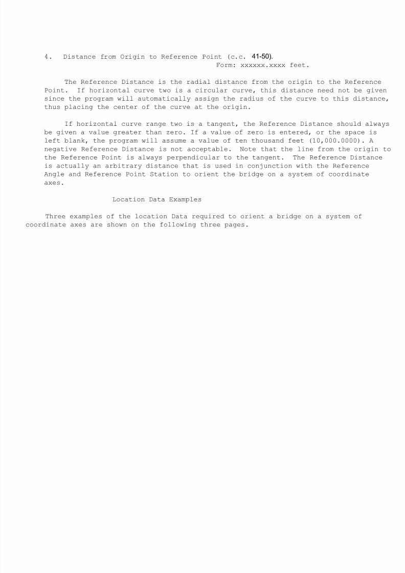
LOCATION DATA
EXAMPLE: 1-1. Layout Data
This example shows how a
bridge is oriented on a system of
coordinate axes. All the stations,
distances, etc., are assumed and
used for the purpose of il-
lustrating the Layout Data input
requirements. Note that the major
portion of the bridge is on a
tangent, and the remaining portionis on a circular curve. The tangent
portion which contains the majority
of the bridge will be set up as
curve two. Therefore, the Reference
Point must be in the tangent
portion. The Reference Point will
be arbitrarily defined as the
intersection point of the survey
lines of the bridge and road
underneath. Note that the skewed
corners at the ends of the bridge
must be taken into account when
selecting the Limiting Stations.
7/21/2019 Georgia Skew
http://slidepdf.com/reader/full/georgia-skew 25/182
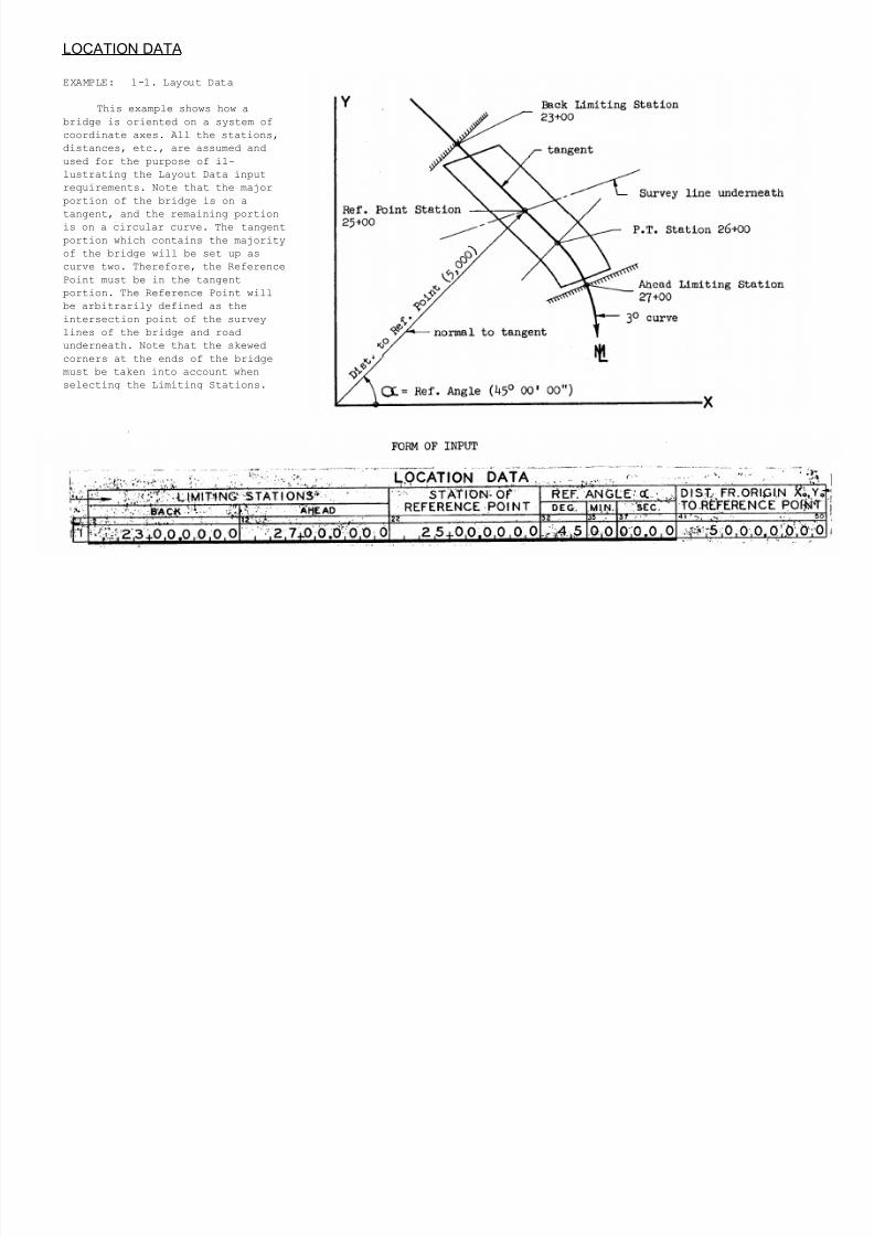
LOCATION DATA (continued)
EXAMPLE 1-2. Layout Data
This example shows how a bridge
that is entirely on a tangent can be
oriented parallel to the Y-axis.
Note that the Reference Angle is
zero in this case. The Station of
the Reference Point is ahead of the
bridge so that all the bridge will
lie in the first quadrant. The
Reference Distance is assumed to be1,000 feet, and the assumed stations
are shown in the sketch.
7/21/2019 Georgia Skew
http://slidepdf.com/reader/full/georgia-skew 26/182
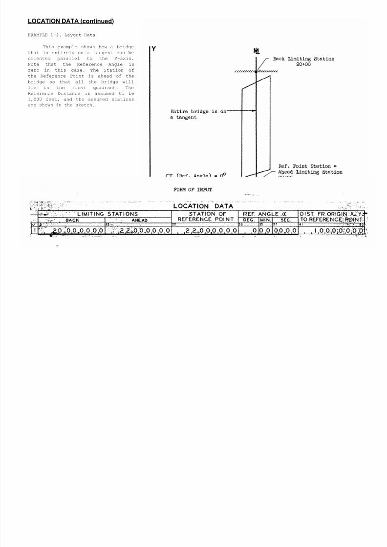
LOCATION DATA (continued)
EXAMPLE 1-3. Layout Data
This example shows how the bents of
a bridge may be set up parallel to the Y-
axis provided, of course, the bents are
parallel. In this case, all the bents are
parallel to the road underneath, which is
common practice. Note that if the Ref.
Angle (α) is made equal to the complement
of the skew angle (Θ), the bents and
survey line underneath will be parallelto the Y-axis. The skew angle should be
known in each case. In this example, a
value of thirty (30) degrees is assumed.
Therefore, the Reference Angle (α) should
have a value of sixty (60) degrees. Note
that the Reference Distance is not
required in this case, i.e., the radius
of the curve will be used as the
Reference Distance.
7/21/2019 Georgia Skew
http://slidepdf.com/reader/full/georgia-skew 27/182
C. HORIZONTAL CURVE DATA (2 in c.c. 1).
Since the bridge may be located in as many as three horizontal curves, the
Horizontal Curve Data is used to enter the degree-of-curvature of each curve, and the
P.C. and P.T. Stations that separate the curve ranges. Note that any of the three
curves may actually be a tangent (straight), i.e., a curve with an infinite radius.
The degree-of-curvature of each range is entered on the input form in degrees,
minutes, and seconds. Note that the curvatures may be entered to the hundredth of a
second. A tangent range of horizontal curve is defined by entering a degree-of-
curvature of zero (0). In actual practice, the bridge will very rarely be on three
ranges of horizontal curves, and bridges on two ranges of horizontal curves are
infrequent. The vast majority of bridges will be completely in only one range of
horizontal curve. Therefore, in order to save the Engineer's time, it is necessary
to define only the ranges of curvature in which the bridge is located. For example,
if the bridge is entirely in one curve (or tangent), only one degree-of-curvature is
required. Likewise, if the bridge is located in two curves (or curve and tangent),
it is necessary to define only two degree-of-curvatures, etc.
Adjoining curves, or adjoining curve and tangent, are assumed to be tangent at
the P.C. and P.T. Stations.
If there is only one range of curvature, it must always be defined as Curve No.
2. In this case, Curve No. 1 and Curve No. 3 would not exist. If there are two
ranges of curvature, one of the ranges must always be defined as Curve No. 2 and the
other curve as either Curve No. 1 or Curve No. 3. For greater program efficiency,,
Curve No. 2 should be the range that contains the major portion of the bridge. This
is the reason that the tangent portion of the bridge in example 1-1 (page 17) was
selected as Curve No. 2.
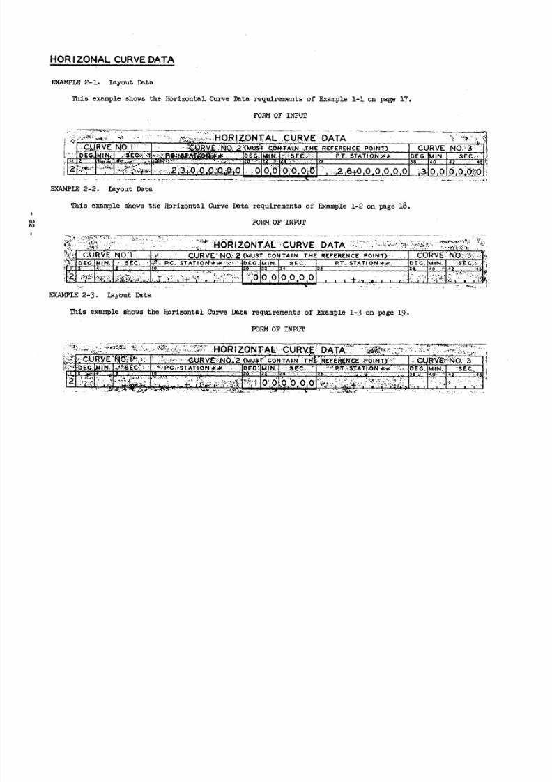
1. Curve No. 1 (c.c. 2-9). Form: xx deg.,xx min.,xx.xx sec.
The degree-of-curvature of curve range one should be entered in this
space. If this curve does not exist, leave this space blank. The beginningstation of Curve No. 1 is assumed to be the Back Limiting Station, and the
ending station is the P.C. Station of curve range two.
2. P.C. Station (c.c. 10-19). Form: xxxx+xx.xxxx feet.
The P.C. Station is the station that begins Curve No. 2 and, therefore,
ends Curve No. 1. This station is not required if only one range of horizontal
curve exists. The program will assign this station the value of the Back
Limiting Station, i.e., the P.C. Station in this case is arbitrary. However,
the P.C. Station should always be given if two or three ranges of horizontal
curvature exist. If Curve No. 1 does not exist when Curve No. 3 does exist,
the P.C. Station can conveniently be set equal to the Back Limiting Station
since the P.C. Station is in this instance an arbitrary station.
7/21/2019 Georgia Skew
http://slidepdf.com/reader/full/georgia-skew 28/182
3. Curve No. 2 (c.c. 20-27). Form: xx deg.,xx min.,xx.xx sec.
This space is for entering the degree-of-curvature of horizontal curve range
two. Curve No. 2 is considered the main curve and, therefore, must always be defined.
The range of Curve Vo. 2 must always contain the Reference Point Station that is
given in the Location Data. The range of Curve No. 2 is from the P.C. Station to the
P.T. Station.
4. P.T. Station (c.c. 28-37). Form: xxxx+xx.xxxx feet.
The P.T. Station is the station that ends the range of Curve No. 2 and begins
Curve No. 3. If only one range (Curve No. 2) of horizontal curve exists, this station
is not required, i.e., leave blank. The program will assign this station the value of
the Ahead Limiting Station, i.e., the P.T. Station in this case is arbitrary.
However, the P.T. Station should always be given if two or three ranges of horizontal
curvature exist. If curve range three does not exist when Curve No. 1 does exist,
the P.T. Station can conveniently be set equal to the Ahead Limiting Station since
the P.T. Station is - in this instance - an arbitrary station.
5. Curve No. 3 (c.c. 38-45). Form: xx deg.,xx min.,xx.xx sec.
Enter in this space the degree-of-curvature of horizontal curve range three. If
this range of mainline curve does not exist, this space should be left blank. The
beginning station of Curve No. 3 is the P.T. Station, and the ending station is
assumed to be the Ahead Limiting Station.
Horizontal Curve Data Examples
The following page contains the Horizontal Curve Data required for the three
examples (1-1, 1-2, 1-3) shown to illustrate the Location Data.
7/21/2019 Georgia Skew
http://slidepdf.com/reader/full/georgia-skew 29/182
7/21/2019 Georgia Skew
http://slidepdf.com/reader/full/georgia-skew 30/182
D. VERTICAL CURVE DATA
The Vertical Curve Data consists of two lines (cards) on the input form. The
first line is for entering P.V.I. Stations; and, the second line is used to enter the
beginning Elevation, Grades (slopes) and Length of Vertical Curves.
1. P.V.I. Stations (3in c.c. l).
The P.V.I. Station is defined as the station of the intersection of the
tangents of a parabolic vertical curve. These stations are required in order
to properly position the vertical curves. The P.V.I. Stations may be of
negative magnitude. These stations should be given on the input form according
to the following requirements.
a. P.V.I. Z Station (c.c. 2-11). Form: xxxx+xx.xxxx feet.
The P.V.I. Z Station is not actually a P.V.I. Station, but rather the
station of the beginning of the Vertical Curve Data. Therefore, this
station must be located before the beginning of the bridge since the
program will not compute the elevation of a point located back of this
station. In essence, this station is the origin of the grade data. The
P.V.I. Z Station should be on a tangent grade and not within a vertical
curve. The P.V.I. Z Station is an arbitrary station and should always be
defined by entering a value on the input form.
The end of the Vertical Curve Data is assumed to be the Ahead
Limiting Station.
b. P.V.I. 1 Station (c.c. 12-21). Form: xxxx+xx.xxxx feet.
If a portion (or all) of the bridge is in a vertical curve, it is
necessary to give as the P.V.I. 1 Station the station of the intersection
of the two grades (Gl and G2) that define the first vertical curve. This
station is not required if the entire bridge is on a tangent.
C. P.V.I. 2 Station (c.c. 22-31). Form: xxxx+xx.xxxx feet.
The program has the capacity for two vertical curves. If a portion
of the bridge lies in a second vertical curve, it is necessary to give as
the P.V.I. 2 Station the station of the intersection of the two grades (G2
and G3) that define the second vertical curve. This station is not
required if the entire bridge is on a tangent, nor when there is only one
vertical curve.
7/21/2019 Georgia Skew
http://slidepdf.com/reader/full/georgia-skew 31/182
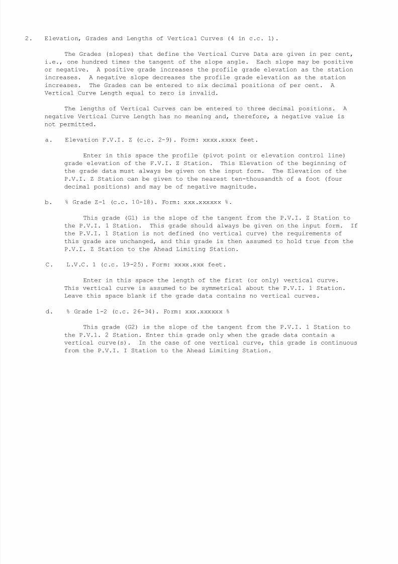
2. Elevation, Grades and Lengths of Vertical Curves (4 in c.c. 1).
The Grades (slopes) that define the Vertical Curve Data are given in per cent,
i.e., one hundred times the tangent of the slope angle. Each slope may be positive
or negative. A positive grade increases the profile grade elevation as the station
increases. A negative slope decreases the profile grade elevation as the station
increases. The Grades can be entered to six decimal positions of per cent. A
Vertical Curve Length equal to zero is invalid.
The lengths of Vertical Curves can be entered to three decimal positions. A
negative Vertical Curve Length has no meaning and, therefore, a negative value is
not permitted.
a. Elevation F.V.I. Z (c.c. 2-9). Form: xxxx.xxxx feet.
Enter in this space the profile (pivot point or elevation control line)
grade elevation of the F.V.I. Z Station. This Elevation of the beginning of
the grade data must always be given on the input form. The Elevation of the
P.V.I. Z Station can be given to the nearest ten-thousandth of a foot (four
decimal positions) and may be of negative magnitude.
b. % Grade Z-1 (c.c. 10-18). Form: xxx.xxxxxx %.
This grade (Gl) is the slope of the tangent from the P.V.I. Z Station to
the P.V.I. 1 Station. This grade should always be given on the input form. If
the P.V.I. 1 Station is not defined (no vertical curve) the requirements of
this grade are unchanged, and this grade is then assumed to hold true from the
P.V.I. Z Station to the Ahead Limiting Station.
C. L.V.C. 1 (c.c. 19-25). Form: xxxx.xxx feet.
Enter in this space the length of the first (or only) vertical curve.
This vertical curve is assumed to be symmetrical about the P.V.I. 1 Station.
Leave this space blank if the grade data contains no vertical curves.
d. % Grade 1-2 (c.c. 26-34). Form: xxx.xxxxxx %
This grade (G2) is the slope of the tangent from the P.V.I. 1 Station to
the P.V.1. 2 Station. Enter this grade only when the grade data contain a
vertical curve(s). In the case of one vertical curve, this grade is continuous
from the P.V.I. I Station to the Ahead Limiting Station.

7/21/2019 Georgia Skew
http://slidepdf.com/reader/full/georgia-skew 32/182
e. L.V.C. 2 (c.c. 35-41). Form: xxxx.xxx feet.
The length of the second vertical curve is entered in this space. However,
if there is no requirement for a second vertical curve, this space should be
left blank. This vertical curve is assumed to be symmetrical about the P.V.I. 2
Station.
f. % Grade 2-3 (c.c. 42-50). Form: xxx.xxxxxx %
This grade (G3) is the slope of the tangent from the P.V.I. 2 Station to
the Ahead Limiting Station and should be entered on the input form only when the
grade data contains two vertical curves.
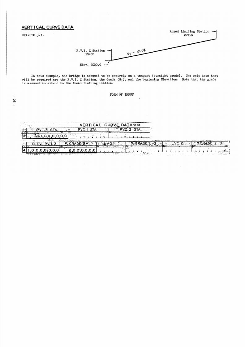
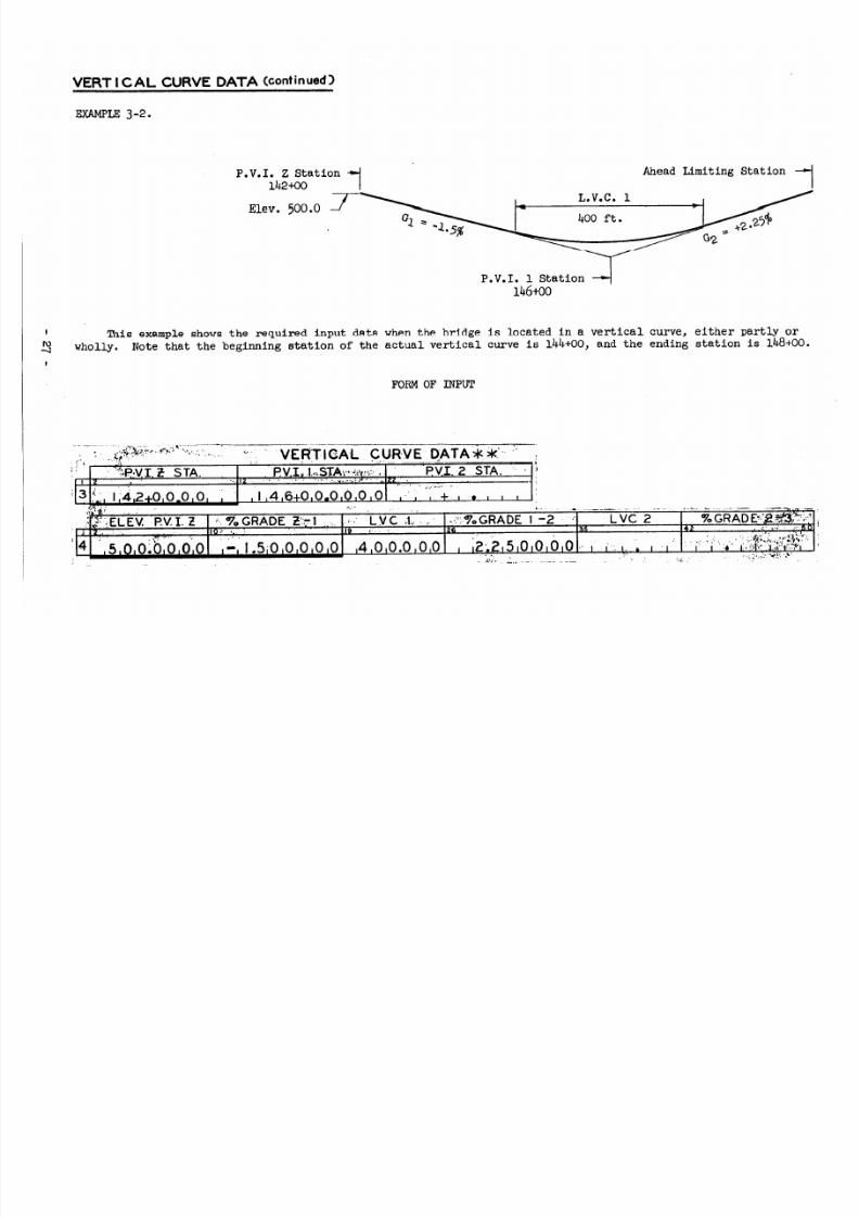
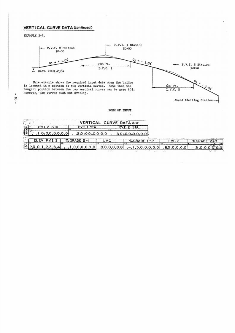
Vertical Curve Data Examples
Three examples of the input data necessary to define the Vertical Curve Data are
shown on the following three pages.
7/21/2019 Georgia Skew
http://slidepdf.com/reader/full/georgia-skew 33/182
7/21/2019 Georgia Skew
http://slidepdf.com/reader/full/georgia-skew 34/182
7/21/2019 Georgia Skew
http://slidepdf.com/reader/full/georgia-skew 35/182
7/21/2019 Georgia Skew
http://slidepdf.com/reader/full/georgia-skew 36/182
E. CROWN AND LANE DEFINITIONS (5 in c.c. 1).
The Crown and Lane Definitions input line is used to enter the data that is
necessary to completely define the type and limits of the transverse bridge surface
(finished grade). The bridge roadway surface may be parabolic, superelevated, or
level (no crown correction). The input form has two formats for reference when
entering the input data. The format used to enter a parabolic crown is the topmost
format to the left, and the superelevated format is immediately below the parabolic
format and encompasses the entire line on the input data form. Since the required
input to define a parabolic crown is entirely different from the data that is
required to define superelevated lanes, the two types of roadway surfaces will be
discussed separately. A level crown is a special case and will be discussed
separately also.
No provision is made for a circular crown; however, a circular
crown can be defined in most cases as a parabola with negligible error.
PARABOLIC CROWN
The program has the capacity for only one parabolic roadway crown, and all
points outside the range of the parabolic surface will be leveled off from the edge
or extent of the parabola. The profile grade control line is assumed to be along the
crown point, i.e., apex of the parabola. The parabolic crown is assumed to be
symmetrical about a vertical axis through the parabola apex.
Card columns 45-79 and 5-12 of the input form should be ignored since no data
is required in these spaces. Also, the Superelevation Data (6 in c.c. 1) which
follows the Crown and Lane Definitions is not required and should be completely
ignored. Following is the required input data for a parabolic crown.
1. Crown Code (c.c. 2-4).
In order to indicate to the computer the type of finished grade surface
the program is to consider, a Crown Code must be given in card columns 2-4 ofthe input form. If the roadway crown is parabolic,, the Crown Code required is
"PAR".
2. Distance From Crown To R/L Gutter (c.c. 13-20). Form: xxxx.xxxx feet.
This dimension is the distance from the apex of the parabola to the extent
of the parabolic surface, usually the gutter line. The distance is measured
perpendicular to the center line of the bridge. This distance is assumed to be
the same for both left and right sides of the bridge and should never be given
a negative value, nor a value of zero. A negative value is meaningless, and a
zero dimension indicates a level crown which can be defined by an easier
method.
7/21/2019 Georgia Skew
http://slidepdf.com/reader/full/georgia-skew 37/182
3. ∆ R From Mainline To Crown (c.c. 21-28). Form: xxxx.xxxx feet.
This dimension is the distance from the mainline (survey control line) to the
apex (crown Point) of the parabolic crown. The distance is measured perpendicular to
the center line of the bridge. This dimension may be negative, zero, or of positive
magnitude. Therefore, the survey line is not required to be along the crown point of
the surface. If the distance from the mainline to the crown point is toward the
origin, the dimension is negative; otherwise (away from origin), the dimension is
positive. Probably, in most cases, the survey line will be along the center line of
the crown surface and, therefore, this dimension will usually be zero.
4. Distance From Crown To Control Point (c.c. 29-36).
Form: xxxx.xxxx feet.
This dimension is the perpendicular distance (horizontal) from the crown point
to a point on the parabolic surface at which the vertical ordinate (drop from crown
point) of the curve is known. This usually turns out to be the gutter line since
most parabolic crowns are detailed at this point. This distance should never be
negative or zero.
5. Drop From Crown To Control Point (c.c. 37-44). Form: xxxx.xxxx inches.
This dimension is the vertical ordinate from the crown point to the point on the
surface at the dimension, "Distance From Crown To Control Point". This dimension
should always be given in INCHES. A value of zero should not be used because this
would define a level crown. A negative value will produce a concave parabola
(sag),and a positive value will produce a convex parabola (hump).
Parabolic Crown Example
An example of a parabolic crown roadway and the required input data is shown on the
following page.
7/21/2019 Georgia Skew
http://slidepdf.com/reader/full/georgia-skew 38/182
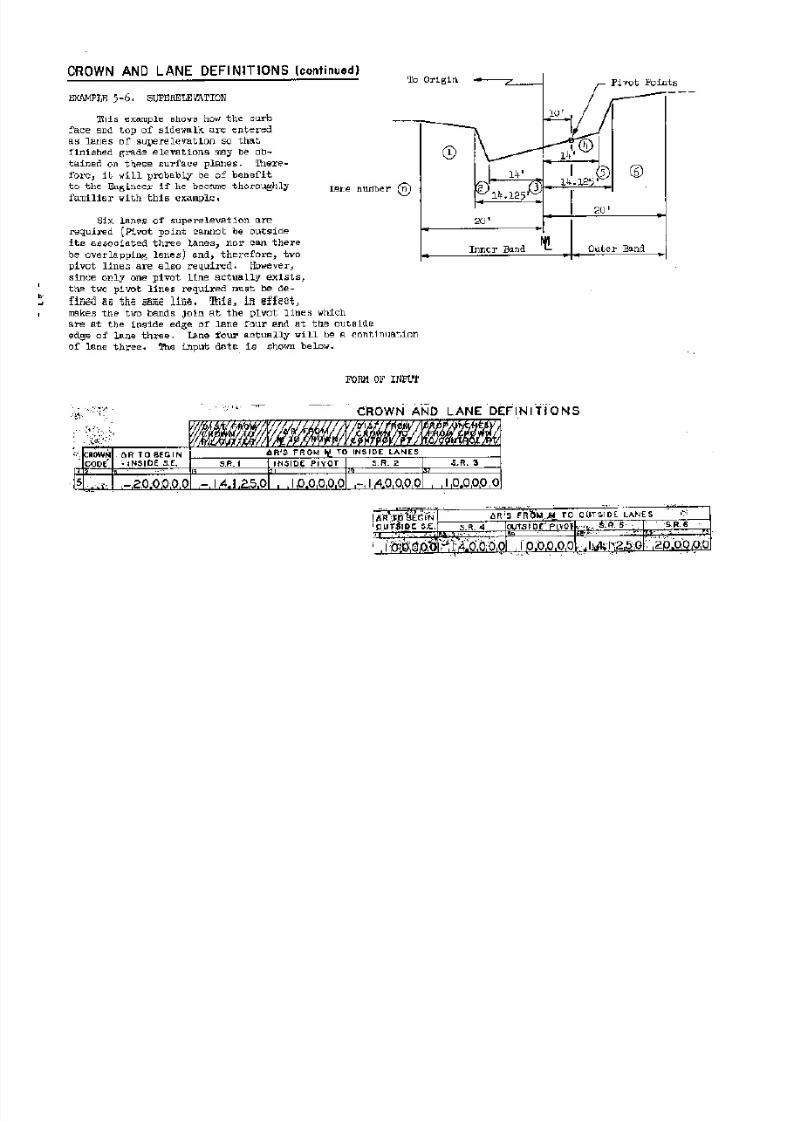
CROWN AND LANE DEFINITIONS
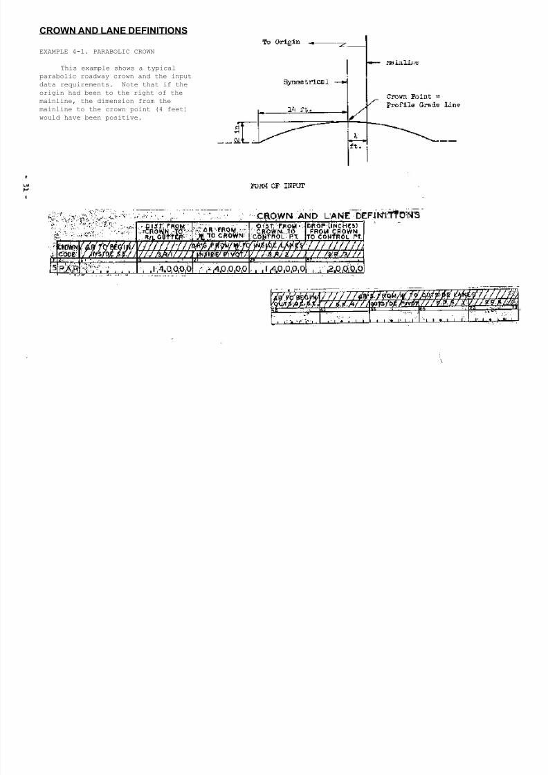
EXAMPLE 4-1. PARABOLIC CROWN
This example shows a typical
parabolic roadway crown and the input
data requirements. Note that if the
origin had been to the right of the
mainline, the dimension from the
mainline to the crown point (4 feet)
would have been positive.
7/21/2019 Georgia Skew
http://slidepdf.com/reader/full/georgia-skew 39/182
SUPERELEVATION
The program has the capacity for six lanes of superelevation which are grouped into
two bands, each containing three adjoining lanes. Each band is controlled independently
by a pivot line; therefore, the bands will not necessarily be adjoining. However, the
vertical curve data is the same for both pivot lines. Three lanes are always associated
with each pivot line even though only one or two may actually exist. When the bridge is
being defined as superelevated, it is required that at least one pivot line and three
lanes be defined. If three lanes are not sufficient, then two pivot lines and six lanes
must be defined. Each pivot line can have no more, or less, than three lanes. When lanes
must be defined that do not actually exist, they can conveniently be given a width of
zero, thus effectively eliminating the lanes.
The innermost (nearest to origin) band of three lanes and pivot line are defined on
the left side of the input form (c.c. 5-44), and the outermost (furthest from origin) band
of three lanes and pivot line are defined on the right side of the input form (c.c. 45-
79). If only three lanes of superelevation are to be defined, the data to define these
lanes should always be entered on the left side of the form, even though all lanes may be
outside the mainline. The terms "inside" and "outside" used on the input form do not
refer to the mainline but rather to the relative position of the bands to the origin. For
instance both bands of superelevated lanes may be totally inside (toward origin) the main-
line or outside (away from origin) the mainline.
The width and position of the lanes of superelevation are defined by giving the
perpendicular or radial distances from the mainline to the edges of the lanes. The
distances are negative if they are measured toward the origin from the mainline, and
positive if they are measured away from the origin from the mainline. All lanes are
assumed to be of constant width throughout the range of the problem, i.e., lanes with
varying widths are not allowed. However, the width of any lane may be different from the
width of any other lane. The pivot line may be in any one of its associated three lanes
of superelevation; however, the pivot line must not be located outside the three lanes.
The position of the mainline relative to the two bands of superelevation is not
restricted. That is, the mainline can be outside, inside, between, or within the twobands of superelevation. If only one band of three lanes is defined,, the relative
position of the mainline is likewise unrestricted.
Each lane of superelevation may have a constant or varying (commonly called
transition) rate of superelevation which is independent of any other lane. The
superelevation rates and transition input data requirements are discussed on page 42.
Following is the input data required to define the lanes of superelevation.
7/21/2019 Georgia Skew
http://slidepdf.com/reader/full/georgia-skew 40/182
1. Crown Code (C.C. 2-4).
In order to indicate to the program that the crown is superelevated, this space
should be left blank, i.e., no particular code is required to define a superelevated
roadway.
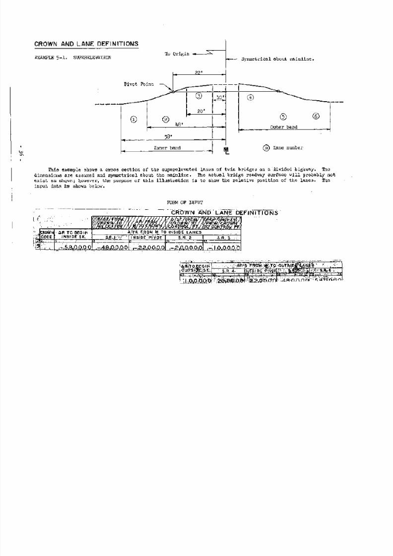
2. ∆ R To Begin Inside S.E. (c.c. 5-12). Form: xxxx.xxxx feet.
This dimension is the distance from the mainline to the inside edge of the
innermost (nearest to origin) lane of superelevation. This distance should always be
given on the input form when the roadway is superelevated. The innermost lane will
be defined as lane one (1) for the purpose of explanation, and each subsequent lane,
moving outward, will be assigned a number in like sequence.
3. S.R. 1 (c.c. 13-20). Form: xxxx.xxxx feet.
The"S.R.1" dimension is the distance from the mainline to the outside edge of
the innermost lane (lane one) and, therefore, to the inside edge of the adjoining
lane (lane two) of superelevation. This dimension is always required with a
superelevated roadway crown and should never be less then the dimension " ∆ R ToBegin Inside S.E.", i.e., overlapping lanes would result in this case. Note that if
the two dimensions,"S.R.1" and "∆ R To Begin Inside S.E. are made equal, the width
of lane one will be zero and, in essence, lane one would not exist.
4. Inside Pivot (c.c. 21-28). Form: xxxx.xxxx feet.
This dimension is the distance from the mainline to the innermost pivot line.
This pivot point must be in lane one, two or three. Since this pivot point must be
within the innermost band of superelevated lanes, the "Inside Pivot" dimension
should not be less than the “∆ R To Begin Inside S.E." dimension, nor greater than
the "S.R.-3"dimension. The pivot point is that point on the superelevated surface
where the Vertical Curve Data holds true. This point or line is also commonly called
the "profile grade line". This dimension should always be given a value on the input
form.
As mentioned before, the bridge roadway may have two pivot lines (twin bridges,
for instance). The pivot line entered here is the one nearest the origin and in the
case of only three lanes, the only pivot line that needs to be defined.
5. S.R. 2 (c.c. 29-36). Form: xxxx.xxxx feet.
The "S.R. 2" dimension is the distance from the mainline to the outside edge of
lane two and, therefore, to the Inside edge of the outside adjoining lane (lanethree). This dimension should always be defined, and the value of the dimension must
never be less than the "S.R. 1" dimension. If the dimensions "S.R. 1" and "S.R. 2" are
made equal, the width of lane two would then be zero and, therefore, lane two would
not actually exist.
7/21/2019 Georgia Skew
http://slidepdf.com/reader/full/georgia-skew 41/182
6. S-R- 3 (c.c. 37-44). Form: xxxx.xxxx feet.
The "S.R. 3" dimension is the distance from the mainline to the outside edge of
lane three. This dimension defines the outer limit of the innermost (or only) band of
superelevated lanes. The "S.R. 3" dimension can be made equal to the "S.R. 2"
dimension to effectively eliminate lane three, but the value of "S.R. 3" should never
be less than "S.R. 2". The "S.R. 3" dimension should always be defined on the input
form with super-elevated roadways.
The preceding dimensions are required to define the position of the inner band (three
lanes) of superelevation. If these three lanes are adequate to fully describe the roadway
surface, the outer band of three lanes need not be defined, i.e., the remainder (c.c. 45-
79) of the input data line should be ignored (left blank). However, sometimes more than
three lanes of superelevation, or two pivot lines, are required to describe the roadway
surface adequately. In this case, the outer band of three superelevated lanes can be used
as follows:
7- ∆ R To Begin Outside S.E. (c.c. 45-51). Form: xxx.xxxx feet.
This dimension is the distance from the mainline to the inside edge of the
innermost lane of the outer band of superelevated lanes and, therefore, the insidelimit of the outer band. This innermost lane of the outer band will be lane four.
Note that lanes three and four are not adjoining lanes. This dimension when defined
must always be equal to, or greater than, the "S.R. 3" dimension previously
discussed.
8. S.R. 4 (c-c- 52-58). Form: xxx.xxxx feet.
The “S.R. 4" dimension is the distance from the mainline to the outside edge of
lane four and, therefore, to the inside edge of the outside adjoining lane (lane 5).
This distance should not be less than the "∆ R To Begin Outside S.E." dimension;
however, the two dimensions can be made equal in order to eliminate lane four when
desired.
9. Outside Pivot (c.c. 59-65). Form: xxx.xxxx feet.
This dimension is the distance from the mainline to the outermost pivot line.
Since the outside pivot point must be within the outer band (lane 4, 5 or 6) of
superelevated lanes, this dimension should not be less than the " ∆ R To Begin
Outside S.E." dimension, nor greater than the "S.R. 6" dimension.
10. S.R. 5 (c.c. 66-72). Form: xxx.xxxx feet.
The "S.R. 5" dimension is the distance from the mainline to the outside edge of
lane five and, therefore, to the inside edge of the outside adjoining lane (lane
six). This distance should never be less than the "S.R. 4" dimension; however, the
two dimensions may be equal in order to eliminate lane five.
7/21/2019 Georgia Skew
http://slidepdf.com/reader/full/georgia-skew 42/182
11. S.R. 6 (c.c. 73-79). Form: xxx.xxxx feet.
The "S.R. 6" dimension is the distance from the mainline to the outside edge of
lane six and, therefore, the outside limit of the outermost band of superelevated
lanes. This dimension may be equal to the "S.R. 5" dimension in order to eliminate
lane six, but never less than that dimension.
For a quick check of the input data (Crown and Lane Definitions) required to define
the superelevated lanes, it should be noted that all dimensions, except the two pivot
dimensions, entered on the input form should be of increasing (or equal) magnitude from
left to right.
NOTE:
Superelevation cannot be used in conjunction with Parabolic Crowns.
Superelevation Examples
Six examples of superelevation lane orientation and the required input data are shown
on the next six pages. Note that the input data are also shown on the input form for
further illustration. It is suggested that these examples be studied thoroughly since this
is perhaps the most difficult aspect of the program to understand.
LEVEL CROWN
If the roadway surface is level, or the crown correction for finished grade elevation
is to be ignored, the only required input is the Crown Code of "LVL" in card columns 2-4.
The rest of the Crown and Lane Definitions input data line should be left blank. In
addition,, the Superelevation Data (6 in c.c. 1) input data lines that immediately follow
the Crown and lane Definitions line should be completely ignored. Note that the number and
position of the lanes of superelevation are immaterial in this instance.
7/21/2019 Georgia Skew
http://slidepdf.com/reader/full/georgia-skew 43/182
7/21/2019 Georgia Skew
http://slidepdf.com/reader/full/georgia-skew 44/182
7/21/2019 Georgia Skew
http://slidepdf.com/reader/full/georgia-skew 45/182
7/21/2019 Georgia Skew
http://slidepdf.com/reader/full/georgia-skew 46/182
7/21/2019 Georgia Skew
http://slidepdf.com/reader/full/georgia-skew 47/182
7/21/2019 Georgia Skew
http://slidepdf.com/reader/full/georgia-skew 48/182
7/21/2019 Georgia Skew
http://slidepdf.com/reader/full/georgia-skew 49/182
F. SUPERELEVATION DATA (6 in c.c. 1).
The Superelevation Data input form line is used to enter the rates of
superelevation of the various superelevated lanes. This data is not required with
Level and Parabolic Crowns and, therefore, this part of the input form would be left
blank. Two types of superelevation may be used to describe the roadway surface:
Constant or Variable (transition) Superelevation. Constant superelevation indicates
that the superelevation rate of each lane remains constant throughout the entire
range of the problem. Transition superelevation indicates the superelevation rate of
a lane, or lanes, varies lineally between two known stations.
It is extremely important that the correct sign be used when entering the
superelevation rates on the input form. If the elevation of the roadway surface
increases as the perpendicular or radial distance from the origin increases, the
superelevation rate is positive. If the elevation decreases as the distance from the
origin increases, the superelevation rate is negative. Note that the superelevation
rates are given in inches per foot. Since the input requirements are somewhat dif-
ferent, the two types of superelevation will be discussed separately.
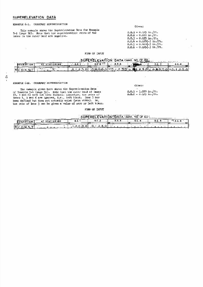
CONSTANT SUPERELEVATION
If the rate of superelevation of all lanes remains constant throughout the
entire bridge, the Superelevation Data should be defined as Constant. Only one line
of the Superelevation Data is required to enter the necessary data.
1. Description (c.c. 2-6).
Th define Constant superelevation., the Description Code "CONST" should be
entered on the first line of the Superelevation Data under the Description
heading.
2. At Station (c-c. 7-16).
This part of the Superelevation Data line should be ignored, i.e., leftblank. The "At Station" data is required only when entering transition
superelevation.
3. Superelevation Rates (c.c. 17-52). Form: xx.xxxx inches per foot.
The input form provides six columns for entering the rate of
superelevation of the lanes. The columns are headed by "S.E. n", where n is the
lane number. For example, the superelevation rate of lane one should be entered
under the column heading "S.E. l” (c.c. 17-22), etc. The superelevation rate
should be given for each lane defined (three or six) in the Crown and Lane
Definitions input line. All rates must be entered on the first line of the
Superelevation Data,, i.e., same line as the Description code "CONST". The
rates of superelevation must be given in units of inches per foot.
Constant Superelevation Examples
The two examples of Constant superelevation are given on the next page for the
purpose of illustration.
7/21/2019 Georgia Skew
http://slidepdf.com/reader/full/georgia-skew 50/182
7/21/2019 Georgia Skew
http://slidepdf.com/reader/full/georgia-skew 51/182
TRANSITION SUPERELEVATION
In order to define Transition Superelevation, the superelevation rate of each
defined lane is required at two or more stations. The rates of superelevation are assumed
to hold true at the defining station only and vary lineally between the stations. It is
required that the station and rate of superelevation for each lane be given at each point
where the rate of transition changes in each lane. In other words, if the rate of
transition changes at a point in any lane, the station and superelevation rate of all the
lanes must be given at that point. The station and superelevation rates at that station
are entered on one line of the Superelevation Data. The input form provides six lines for
entering up to six stations. However, the program capacity is ten stations. Should more
than six stations be required, extra lines may be added to the bottom of the input form.
The input requirements are as follows;
1. Description (c.c. 2-6).
In order to indicate to the program that Transition Superelevation is to be
entered in the Superelevation Data, the Description code "START" must be entered on
the first line of the Superelevation Data under the heading "Description". The
Description code "FINIS" is required on the last line of data (station and
superelevation rates) entered in the Superelevation Data. The Description code should
be left blank on all lines used to enter intermediate stations, i.e., stations
between the first (beginning) station and the last (ending) station. Therefore, the
Description codes "START" and "FINIS" are entered only once. The Description code
"CONST" should not be used with Transition superelevation. No other Description codes
are valid.
2. At Station (c.c. 7-16). Form: xxxx+xx.xxxx feet.
This column is for entering the station of each break (change) in
superelevation transition. The initial station which is entered on the first line
must be back of the beginning of the bridge since the superelevation rates are not
known back of the initial station, i.e., the program does not assume that the
superelevation rates back of the initial station are the same as the rates at theinitial station. The last station entered must be ahead of the end of the bridge
since the superelevation rates are not known ahead of the last station, i.e., the
program does not assume that the superelevation rates ahead of the last station are
the same as the rates at the last station.
A maximum of ten stations can be used to define the transition sequence.
However, only six lines are provided on the input form. The stations may be of
negative magnitude.
3. Superelevation Rates (c.c. 17-52). Form: xx.xxxx inches per foot.
The rate of superelevation of each lane defined in the Crown and Lane
Definitions input data must be given at each station of transition break that isentered in the Superelevation Data., i.e., At Stations.

7/21/2019 Georgia Skew
http://slidepdf.com/reader/full/georgia-skew 52/182
Six columns are provided on the input form to enter the rate of superelevation
of the lanes. The number in each heading indicates which lane of superelevation is to
be entered in that column. For example, the superelevation rates of lane five are
entered in the column headed by "S.E. 5".
NOTE:
Superelevation defined as Constant cannot be used in conjunction with superelevation
defined as Transition.
Transition Superelevation Examples
Four examples of the method of entering Transition superelevation on the input
data form are given on the following four pages for the purpose of illustration only.
The examples do not represent actual cases of bridge transition.
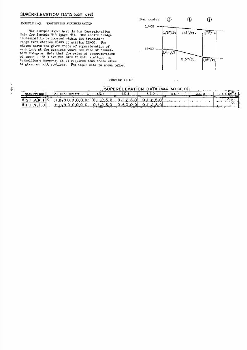
7/21/2019 Georgia Skew
http://slidepdf.com/reader/full/georgia-skew 53/182
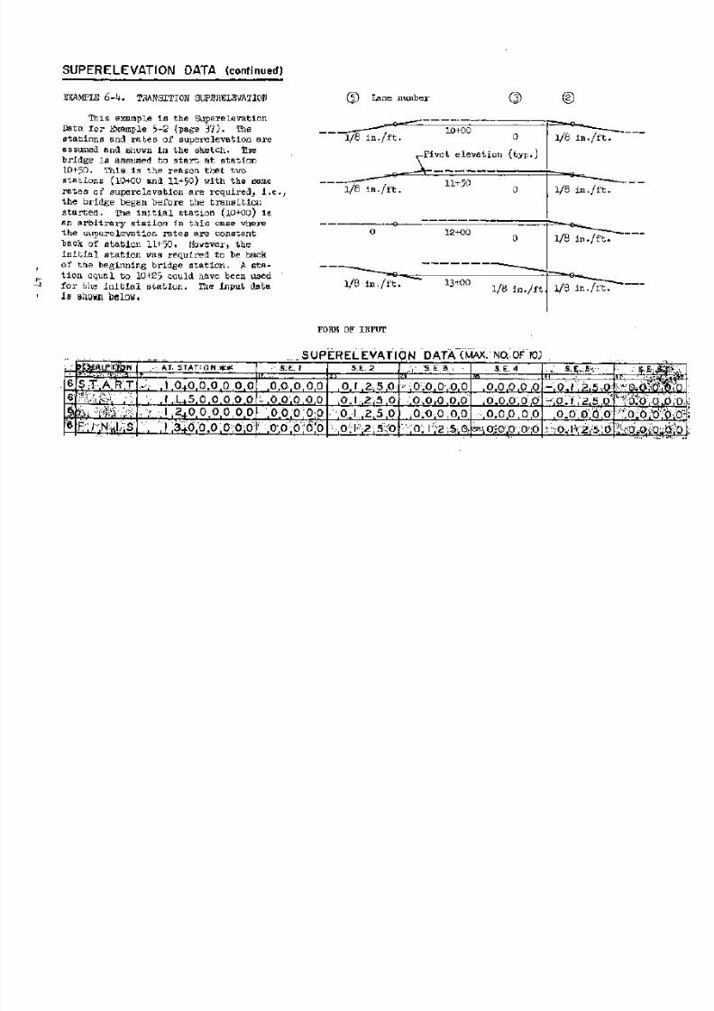
7/21/2019 Georgia Skew
http://slidepdf.com/reader/full/georgia-skew 54/182
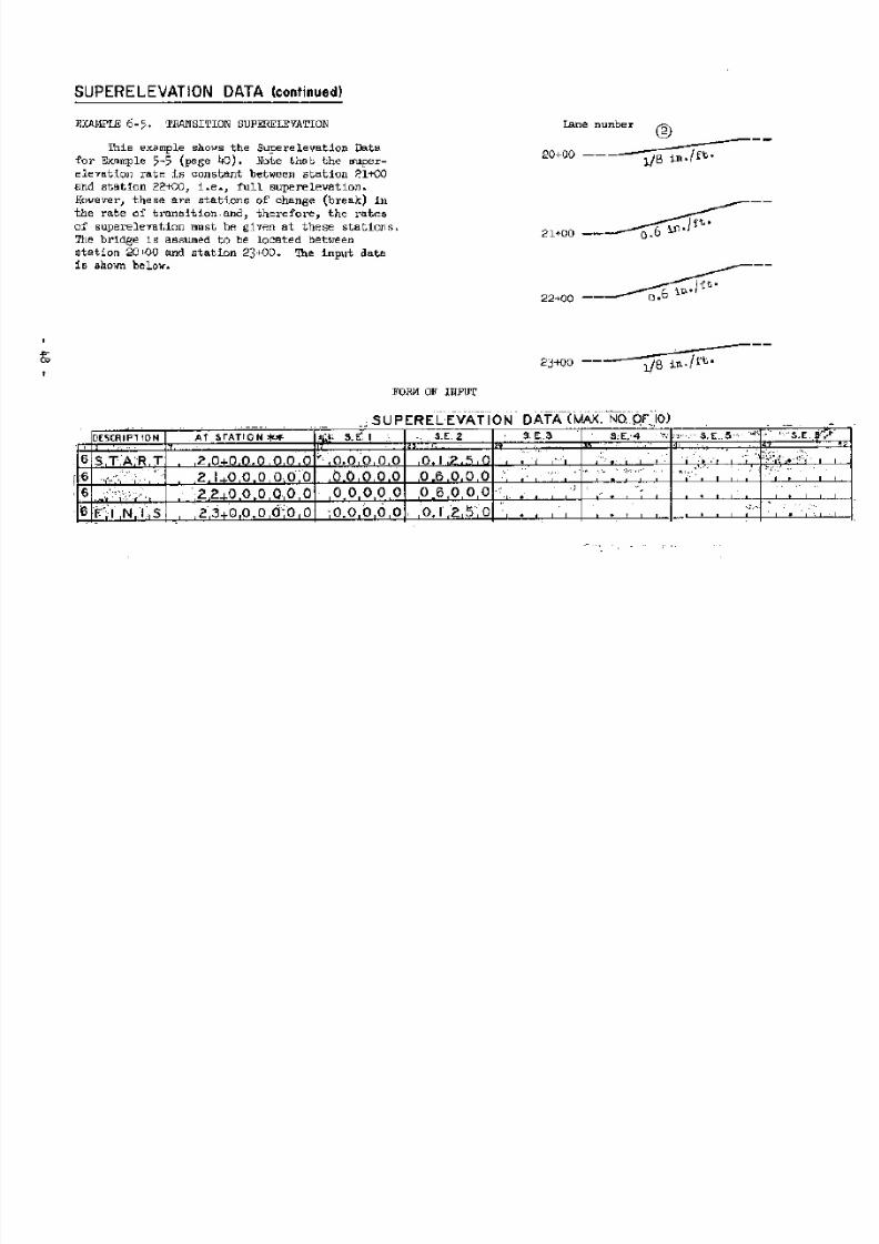
7/21/2019 Georgia Skew
http://slidepdf.com/reader/full/georgia-skew 55/182
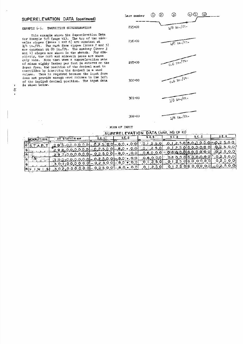
7/21/2019 Georgia Skew
http://slidepdf.com/reader/full/georgia-skew 56/182
7/21/2019 Georgia Skew
http://slidepdf.com/reader/full/georgia-skew 57/182
LONGITUDINAL LINES
The LONGITUDINAL LINES input form is used to define longitudinal lines that the
Engineer desires to be intersected with the bents and transverse lines of each span. This
input form must always be used with each problem, and at least one longitudinal line must
be defined on the sheet. This input form is required as the second sheet of each problem,
immediately following the LAYOUT DATA input form. Usually only one sheet of this type is
required per problem. However, on occasions the need will arise for a different set of
longitudinal lines within the same problem. For example, the number of beams may vary from
span to span. For illustration, let's assume a bridge has five spans, and the first two
spans have five beams and the remaining three spans have four beams. A set of longitudinal
lines will be used with the first two spans. and a different set of longitudinal lines
with the last three spans. In this example, the second set of longitudinal lines must
immediately follow the SPAN DATA input sheet of span two and immediately precede the SPAN
DATA input form for span three. In other words, the longitudinal lines for a span or spans
must immediately precede the input data for those spans. Whenever a set of longitudinal
lines are given in the input data of a problem, they completely replace the previous
longitudinal lines. Any lines common to both sets of longitudinal lines must be redefined.
The program has the capacity for thirty (30) longitudinal lines. Each longitudinal
line is defined by entering the required input data on one line of the input form. Note
that a Sequence Number is given in card columns 2 and 3. These numbers will be assigned to
the longitudinal lines. For instance, the longitudinal line entered on the fourth line (04
in c.c. 2, 3) of the input form will be longitudinal line number four (4). The
longitudinal lines should be defined by entering the first longitudinal line on the first
input line and continuing with one longitudinal line per input line. Lines on the form
should not be skipped, i.e., no blank lines are allowed between the longitudinal lines
defined on the form. This is required because the longitudinal lines must be in numerical
sequence.
Immediately after entering the last longitudinal line, the code "END" must always be
entered in card columns 4-6 (Type Code) of the next input line. The total number of lines
of the input form that must contain data is the number of longitudinal lines (which may
vary from one to thirty) plus one (the line that contains the "END" code). All remaininglines of the input form should be left blank.
The order in which the longitudinal lines are listed on the input form is
immaterial. However, as a general rule, the longitudinal lines should be given in some
sort of location sequence, i.e., from left to right, or right to left, across the bridge.
After the user becomes familiar with the program, he will be able to give the longitudinal
lines in the order that will be most beneficial to him. The Engineer should be thoroughly
familiar with the "Distance To Previous Point" dimension (page 120) that is given in the
output data before selecting the order of the longitudinal lines.
7/21/2019 Georgia Skew
http://slidepdf.com/reader/full/georgia-skew 58/182
Ten types of longitudinal lines are available to the user. Following is a list of
the different types of longitudinal lines:
1. Chord
2. Arc
3. Railing
4. Parallel
5. Parallel thru Intersect Ahead
6. Parallel thru Intersect Back
7. Curve Offset
8. Straight Taper
9. Curve Taper
10. Coordinate
Following is a discussion of the input data that is common to all longitudinal
lines.
1. Skip Code (c.c. 49).
Sometimes a longitudinal line must be defined solely for the purpose of
being a reference line, i.e., a line from which some other longitudinal line is
referred (dimensioned). In this case, it may not be desirable to have the
intersection data of this longitudinal line in the output data. Therefore, to
eliminate a longitudinal line from the output data, the digit one (1) should be
entered in the Skip code column. Otherwise, this card column should be leftblank to obtain this intersection data in the output.
2. Remarks (c.c. 50-6o).
This space is for entering any identifying and pertinent Remarks which
describe each longitudinal line. These Remarks will appear with the
longitudinal line in the output data. It is suggested that Remarks be used
freely so that the longitudinal lines may be readily recognized in the output
data.
Following is a discussion of each type of longitudinal line which
includes the usage, the required input data, a sketch., and example of each type.
7/21/2019 Georgia Skew
http://slidepdf.com/reader/full/georgia-skew 59/182
A. CHORD
A Chord is by definition a straight line that joins two points on a circle.
Therefore, a Chord longitudinal line is a straight line between two points on a
curve that is concentric with the mainline. The two points that define the chord
longitudinal line are the points of intersection of the concentric circle with the
two defining bents (Ahead and Back) of each span. Therefore, the chord longitudinal
line will vary from span to span if the mainline is a circular curve, i.e., the
chord longitudinal line will not be a continuous straight line, but rather a series
of straight segments (chords). If the mainline is a tangent, the chord becomes a
continuous straight line parallel to the mainline. Vote that a chord longitudinal
line is directly dependent on the type of mainline curve (tangent or circular).
If a bridge is on a curve, it is common practice to place the beams on chords
of concentric circles with the mainline. The primary purpose of the chord
longitudinal line is to define such a beam line. A chord longitudinal line may also
be used solely as a reference line, i.e., so other lines may be made parallel to the
chord. An example of this is when all the beams in a span are made parallel to a
chord of the centerline arc. In this case, a chord longitudinal line of the
centerline must be set up so that the beam lines may be referenced (made parallel)
to the chord. If there is no beam on the centerline arc, then the chord is actually
being used for reference only. If the mainline is a tangent, the chord longitudinal
line may be used to represent other lines, i.e., gutter, curb, centerline, and
structure limit lines.
Structure limit lines are such lines as the outside edges of the roadway slab
or the outside edge of the sidewalks, etc.
Any number (thirty or less) of chord longitudinal lines may be defined and used
in conjunction with all other types of longitudinal lines. Following are the
required input data for defining chord longitudinal lines.
1. Type Code (c.c. 4-6).
The code "CRD" is used to define a chord longitudinal line. This code is
required with every chord line entered on the input form.
2. Ref. Call (c-c- 7, 8).
The Reference Call is not required with longitudinal lines defined as
chords. The chord longitudinal line is always assumed to be referenced from the
mainline. Therefore, the Reference Call should be left blank.
3. AR From Mainline (c.c. 9-18). Form: xxxxxx.xxxx feet.
This dimension is the radial or perpendicular distance from the mainline
to the concentric circular arc of which the longitudinal line is a chord. Ifthe concentric arc is inside (toward origin) the mainline, the dimension is
negative. If the concentric arc that defines the chord is outside (away from
origin) the mainline, this dimension is positive.
Card columns 19-48 of the input form should be left blank when defining a chord
longitudinal line, i.e., no input data is required in these card columns. The Skip code
(c.c. 49) and Remarks (c.c. 50-80) are discussed on page 51. An example showing how the
chord longitudinal line data is entered on the input form is shown on pages 74 and 75.
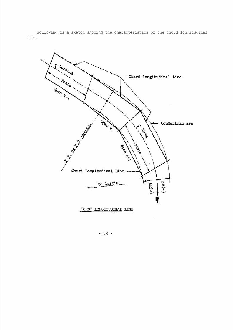
7/21/2019 Georgia Skew
http://slidepdf.com/reader/full/georgia-skew 60/182
Following is a sketch showing the characteristics of the chord longitudinal
line.
7/21/2019 Georgia Skew
http://slidepdf.com/reader/full/georgia-skew 61/182
B. ARC
An arc is by definition a portion of a circular curve. Therefore, an arc
longitudinal line is a circular curve that is concentric with the mainline. The arc
line will be a continuous line throughout the range of the bridge. However, if the
mainline is a tangent, the arc longitudinal line will actually be a straight line
parallel to the mainline. Note that the arc line is always the same type (circular or
straight) line as the mainline.
If a bridge is on a curve, it is common practice to make the curb, gutter, and
structure lines concentric with the mainline curve. These lines can be defined as arc
longitudinal lines; in addition, the centerline or survey line (mainline) may be
defined as an arc. The arc line may be used as a reference line by a Railing
longitudinal line. Curved girders can also be represented by arc lines. Any number
(thirty or less) of arc longitudinal lines may be defined and used in conjunction
with all other types of longitudinal lines. Following is the required input data for
defining arc longitudinal lines.
1. Type Code (c.c. 4-6).
The code "ARC" is used to define an arc longitudinal line. This code is
required with every arc line entered on the input form.
2. Ref. Call (c.c. 7, 8).
The Reference Call is not required with longitudinal lines defined as
arcs. The are longitudinal line is always assumed to be referenced from the
mainline. Therefore, the Reference Call should be left blank.
3. ∆ R From Mainline (c.c. 9-18). Form: xxxxxx.xxxx feet.
This dimension is the radial or perpendicular distance from the mainline
to the concentric arc. If this dimension is measured toward the origin, the
distance is negative. Otherwise, the distance is positive (outside mainline).
Card columns 19-48 of the input form should always be left blank when defining
an arc line. The Skip code (c.c. 49) and Remarks (c.c. 5080) are discussed on page
51. An example showing how the arc longitudinal line data is entered on the input
form is shown on page 74.
On the following page is a sketch showing the characteristics of the arc
longitudinal line.
7/21/2019 Georgia Skew
http://slidepdf.com/reader/full/georgia-skew 62/182
7/21/2019 Georgia Skew
http://slidepdf.com/reader/full/georgia-skew 63/182
C. RAILING
The railing line is a longitudinal line that is the same type as some other
longitudinal line from which the railing line is referenced. For example, if a
railing line is referenced to an arc longitudinal line, the railing line will be an
arc line. If a railing line is referenced to a curve taper longitudinal line, the
railing line will be a curve taper line, etc. However, there is one characteristic of
the railing line that is different from the longitudinal line from which it is ref-
erenced. That is, the bent and transverse lines may be intersected with a railing
line, or the bent and transverse lines may be intersected with the longitudinal line
to which the railing is referenced and then turned radially to intersect the railing
line. The sketch clearly shows this optional feature of the railing line. The option
of which intersection the program is to consider is controlled by the bent and
transverse line input data which will be discussed on subsequent pages.
The railing line is used to enter the sidewalk railing (for railing post
spacings) and structure lines (elevations for construction) since the sidewalk
construction joints are usually radial to the gutter line. Therefore, if a railing
line is referenced to the longitudinal line that represents the gutter line, the bent
and transverse lines may be intersected with the railing by turning radially from
their intersection with the gutter line. If both points (see sketch) of intersection
are desired in the output data, the railing or structure line must be defined twice,
i.e., once as a railing longitudinal line and again as another type of longitudinal
line (arc, curve taper, etc.). Note that when a bent or transverse line is coded to
intersect a railing without turning radially from another longitudinal line, the bent
or transverse line will intersect all railing lines in like fashion.
Any number of railing longitudinal lines may be defined and used in conjunction
with all other types of longitudinal lines. However, some other type of longitudinal
line must always be defined when using railing lines so that the railing lines may
be referenced to the other type of longitudinal line. Railing lines should not be
referenced to chord longitudinal lines when the mainline is a circular curve.
Following is the required input data for defining railing longitudinal lines.
1. Type Code (c.c. 4-6).
The code "RLG" is used to define a railing longitudinal line. This code is
required with every railing line entered on the input form.
2. Ref. Call (c.c. 7, 8). Form: xx.
The Reference Call is the Sequence Number (c.c. 2-3) of the longitudinal
line to which the railing line is referenced. The Reference Call must always be
given when defining a railing longitudinal line. The Reference Call must not be
the Sequence Number of a longitudinal line that is referenced (has a Ref. Call)
to some other longitudinal line. Therefore, the railing line cannot be
referenced to the following types of longitudinal lines:
1. Railing
2. Parallel
3. Parallel thru Intersect Ahead
4. Parallel thru Intersect Back

7/21/2019 Georgia Skew
http://slidepdf.com/reader/full/georgia-skew 64/182
No other type of longitudinal line may be referenced to a railing longitudinal
line because the railing longitudinal line has a Reference Call. The railing line
Reference Call cannot be zero or blank, nor can the Reference Call be greater than
the total number of longitudinal lines. In addition, the Reference Call cannot be
equal to the Sequence Number of the railing line.
7/21/2019 Georgia Skew
http://slidepdf.com/reader/full/georgia-skew 65/182
3. ∆ R From Reference Line (c.c. 9-18). Form: xxxxxx.xxxx feet.
This dimension is the radial or perpendicular distance from the reference line
of the railing (another longitudinal line) to the railing line. Note that the railing
line is not referenced from the mainline. If the distance is measured toward the
origin from the reference line, the dimension is negative; otherwise (away from theorigin), the dimension is positive.
Card columns 19-48 of the input form should be ignored when defining railing
longitudinal lines. The Skip code (c.c. 49) and Remarks (c.c. 50-8o) are discussed on page
51. An example showing how the railing longitudinal line data is entered on the input form
is shown on page 74.
On the following page is a sketch showing the characteristics of the railing
longitudinal line.
NOTE: The same railing can be defined more than one time in one set of
longitudinal lines, and each time the railing is defined a different
reference line can be used. This may be advantageous when the transverselines turn radially from different railing reference lines to intersect
the railing line.
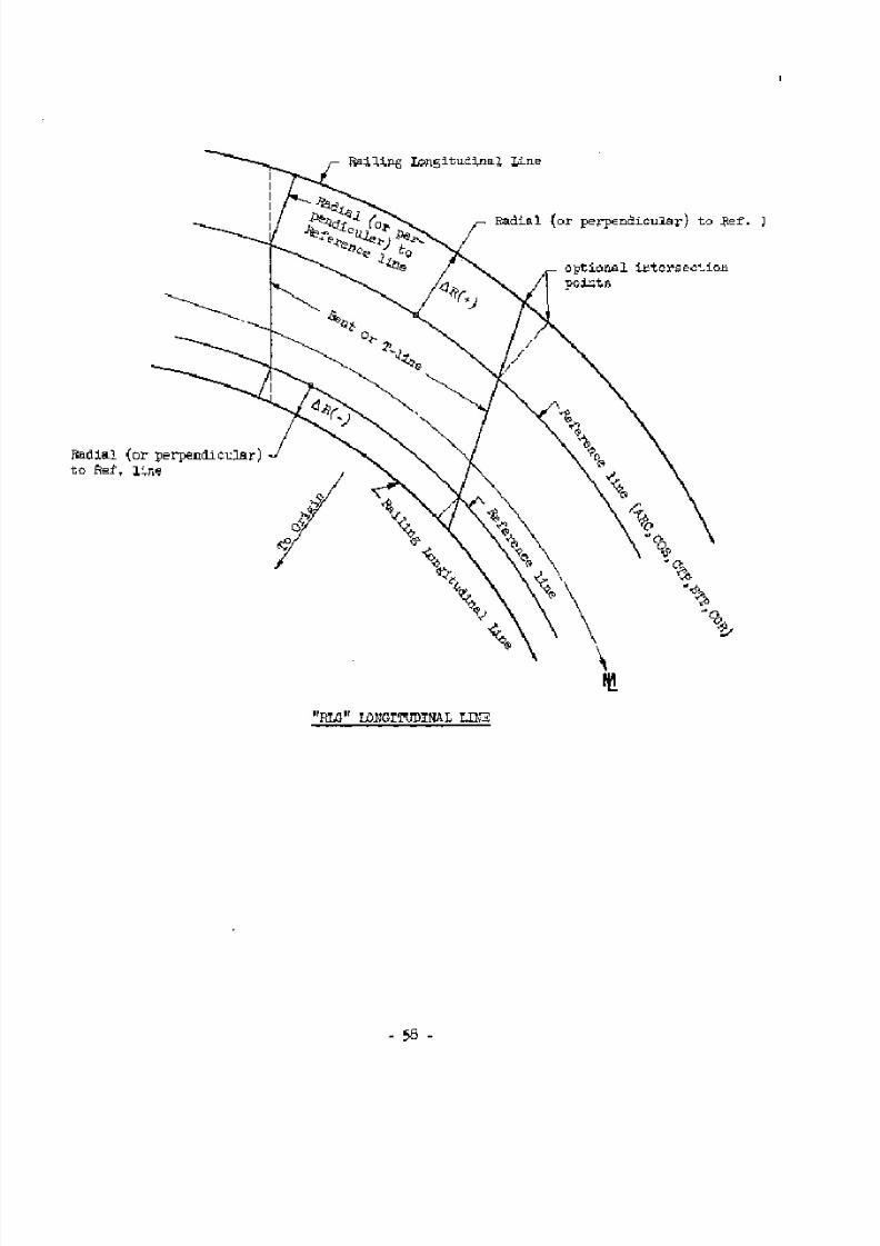
7/21/2019 Georgia Skew
http://slidepdf.com/reader/full/georgia-skew 66/182
7/21/2019 Georgia Skew
http://slidepdf.com/reader/full/georgia-skew 67/182
D. PARALLEL
A parallel longitudinal line is a straight line that is parallel to some other
longitudinal line (reference line). The reference line of the parallel longitudinal
line must be a straight line, i.e., chord, straight taper or coordinate longitudinal
line. If the parallel line is referenced to a chord longitudinal line, the parallel
line will be a series of straight lines parallel to the chord line segments. If the
parallel line is referenced to a straight taper or coordinate, the parallel line will
be a straight line continuous throughout the range of the problem.
A parallel line cannot be referenced to a longitudinal line that is referenced
to some other longitudinal line. Therefore, the following types of longitudinal lines
cannot be used as a reference line for a parallel longitudinal line, since each line
requires a reference line or the line is always a curve.
1. Railing
2. Parallel
3. Parallel thru Intersect Ahead
4. Parallel thru Intersect Back
5. Curve Offset
6. Curve Taper
A parallel line may be referenced to an arc longitudinal line provided the mainline
is a tangent throughout the range of the problem, i.e., the arc line in this case
would be a straight line.
It is common practice to make all the beams in a span on a horizontal curve
parallel for simplicity in detailing and construction. The parallel longitudinal line
can be used to define such beam lines. However, it is important to note that theparallel lines of adjacent spans if referenced to chords will not necessarily join at
the bent that separates the spans. Parallel lines may also be used for curb, gutter
and structure lines if the mainline is a tangent throughout the range of the bridge.
Any number of parallel longitudinal lines may be defined and used in conjunction
with all other types of longitudinal lines. However, some other type of longitudinal
line must always be defined when using parallel lines so that the parallel lines can
be referenced to the other type of longitudinal line. Following is the required input
data for defining parallel longitudinal lines.
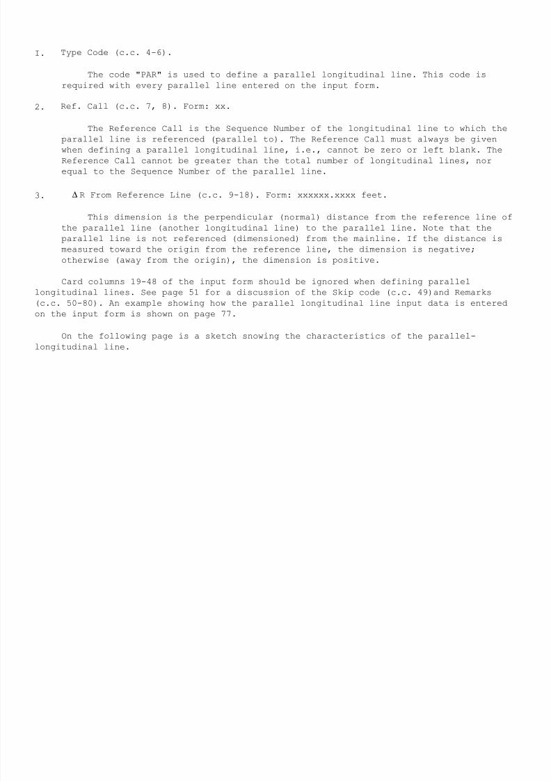
7/21/2019 Georgia Skew
http://slidepdf.com/reader/full/georgia-skew 68/182
I. Type Code (c.c. 4-6).
The code "PAR" is used to define a parallel longitudinal line. This code is
required with every parallel line entered on the input form.
2. Ref. Call (c.c. 7, 8). Form: xx.
The Reference Call is the Sequence Number of the longitudinal line to which the
parallel line is referenced (parallel to). The Reference Call must always be given
when defining a parallel longitudinal line, i.e., cannot be zero or left blank. The
Reference Call cannot be greater than the total number of longitudinal lines, nor
equal to the Sequence Number of the parallel line.
3. ∆ R From Reference Line (c.c. 9-18). Form: xxxxxx.xxxx feet.
This dimension is the perpendicular (normal) distance from the reference line of
the parallel line (another longitudinal line) to the parallel line. Note that the
parallel line is not referenced (dimensioned) from the mainline. If the distance is
measured toward the origin from the reference line, the dimension is negative;
otherwise (away from the origin), the dimension is positive.
Card columns 19-48 of the input form should be ignored when defining parallel
longitudinal lines. See page 51 for a discussion of the Skip code (c.c. 49)and Remarks
(c.c. 50-80). An example showing how the parallel longitudinal line input data is entered
on the input form is shown on page 77.
On the following page is a sketch snowing the characteristics of the parallel-
longitudinal line.
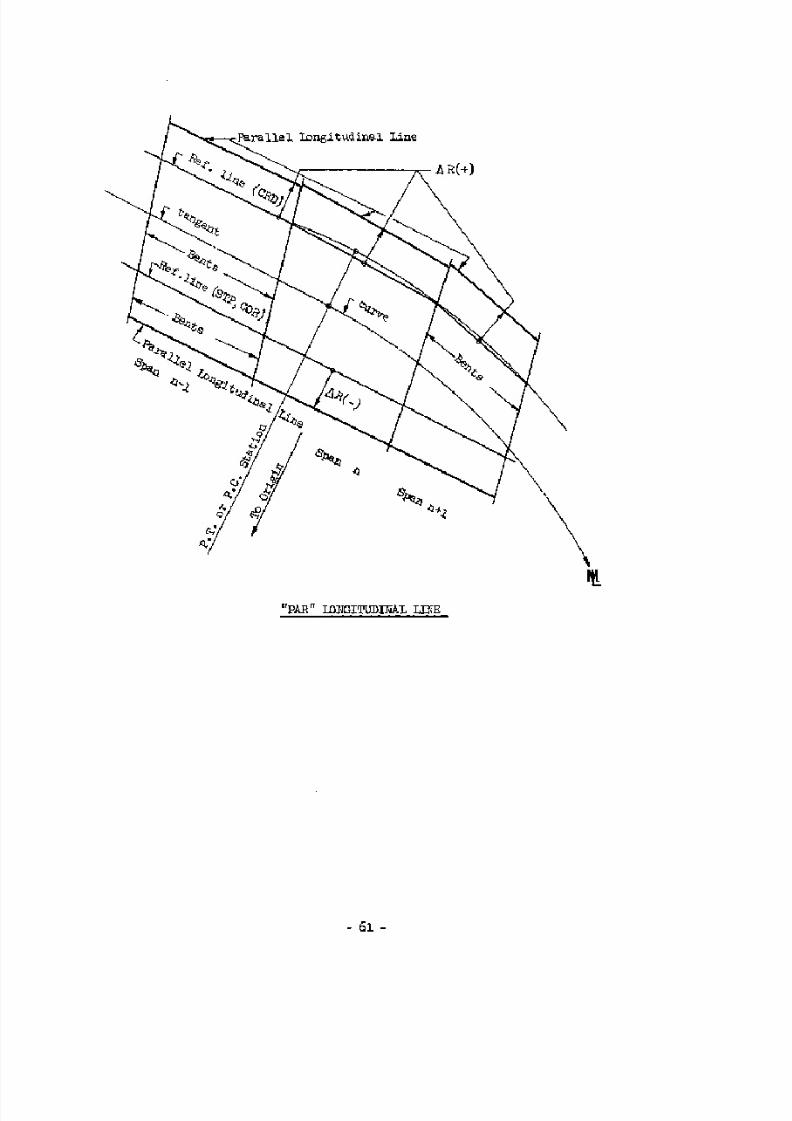
7/21/2019 Georgia Skew
http://slidepdf.com/reader/full/georgia-skew 69/182
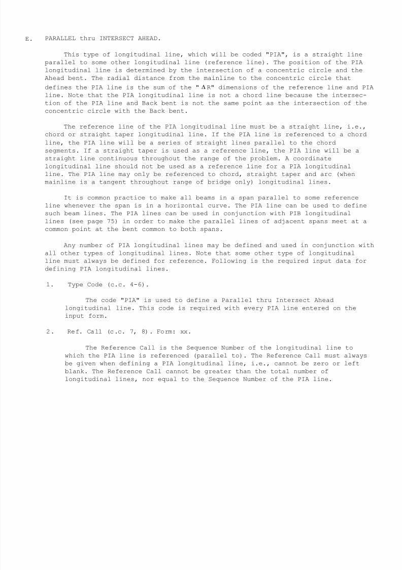
7/21/2019 Georgia Skew
http://slidepdf.com/reader/full/georgia-skew 70/182
E. PARALLEL thru INTERSECT AHEAD.
This type of longitudinal line, which will be coded "PIA", is a straight line
parallel to some other longitudinal line (reference line). The position of the PIA
longitudinal line is determined by the intersection of a concentric circle and the
Ahead bent. The radial distance from the mainline to the concentric circle that
defines the PIA line is the sum of the "∆ R" dimensions of the reference line and PIA
line. Note that the PIA longitudinal line is not a chord line because the intersec-
tion of the PIA line and Back bent is not the same point as the intersection of the
concentric circle with the Back bent.
The reference line of the PIA longitudinal line must be a straight line, i.e.,
chord or straight taper longitudinal line. If the PIA line is referenced to a chord
line, the PIA line will be a series of straight lines parallel to the chord
segments. If a straight taper is used as a reference line, the PIA line will be a
straight line continuous throughout the range of the problem. A coordinate
longitudinal line should not be used as a reference line for a PIA longitudinal
line. The PIA line may only be referenced to chord, straight taper and arc (when
mainline is a tangent throughout range of bridge only) longitudinal lines.
It is common practice to make all beams in a span parallel to some referenceline whenever the span is in a horizontal curve. The PIA line can be used to define
such beam lines. The PIA lines can be used in conjunction with PIB longitudinal
lines (see page 75) in order to make the parallel lines of adjacent spans meet at a
common point at the bent common to both spans.
Any number of PIA longitudinal lines may be defined and used in conjunction with
all other types of longitudinal lines. Note that some other type of longitudinal
line must always be defined for reference. Following is the required input data for
defining PIA longitudinal lines.
1. Type Code (c.c. 4-6).
The code "PIA" is used to define a Parallel thru Intersect Aheadlongitudinal line. This code is required with every PIA line entered on the
input form.
2. Ref. Call (c.c. 7, 8). Form: xx.
The Reference Call is the Sequence Number of the longitudinal line to
which the PIA line is referenced (parallel to). The Reference Call must always
be given when defining a PIA longitudinal line, i.e., cannot be zero or left
blank. The Reference Call cannot be greater than the total number of
longitudinal lines, nor equal to the Sequence Number of the PIA line.
7/21/2019 Georgia Skew
http://slidepdf.com/reader/full/georgia-skew 71/182
3. ∆ R From Reference Line (c.c. 9-18). Form: xxxxxx.xxxx feet.
This dimension is the radial distance from the concentric circle that defines
the reference line to the concentric circle that locates the intersection of the PIA
line with the Ahead bent. If the distance is measured toward the origin, the
dimension is negative. If the distance is measured away from the origin, the
dimension is positive.
Card columns 19-48 of the input form should be left blank when defining PIA
longitudinal lines. See page 51 for a discussion of the Skip code (c.c. 49) and Remarks
(c.c. 50-80). An example showing how the PIA longitudinal line input data is entered on
the input form is shown on page 76.
Following is a sketch showing the characteristics of the PIA longitudinal line.
7/21/2019 Georgia Skew
http://slidepdf.com/reader/full/georgia-skew 72/182
F. PARALLEL thru INTERSECT BACK
This type of longitudinal line, which will be coded "PIB", is a straight line
parallel to some other longitudinal line (reference line). The position of the PIB
longitudinal line is determined by the intersection of a concentric circle and the
Back bent. The radial distance from the mainline to the concentric circle that
defines the FIB line is the sum of the "∆ R" dimensions of the reference line and
PIB line. Note that the PIB longitudinal line is not a chord line because the
intersection of the PIB line and Ahead bent is not the same point as the inter-
section of the concentric circle with the Ahead bent.
The reference line of the PIB longitudinal line must be a straight line, i.e.,
chord or straight taper longitudinal line. If the PIB line is referenced to a chord
line, the PIB line will be a series of straight lines parallel to the chord
segments. If a straight taper is used as a reference line, the PIB line will be a
straight line continuous throughout the range of the problem. A coordinate
longitudinal line should not be used as a reference line for a PIB longitudinal
line. The PIB line may only be referenced to chord, straight taper and arc (when
mainline is a tangent throughout range of bridge only) longitudinal lines.
It is common practice to make all beams in a span parallel to some referenceline whenever the span is in a horizontal curve. The PIB line can be used to define
such beam lines. The PIB lines can be used in conjunction with PIA longitudinal
lines (see page 75) in order to make the parallel lines of adjacent spans meet at a
common point at the bent common to both spans.
Any number of PIB longitudinal lines may be defined and used in conjunction with
all other types of longitudinal lines. Note that some other type of longitudinal
line must always be defined for reference. Following is the required input data for
defining PIB longitudinal lines.
1. Type Code (c.c. 4-6).
The code "PIB" is used to define a Parallel thru Intersect Backlongitudinal line. This code is required with every PIB line entered on the
input form.
2. Ref. Call (c.c. 7, 8). Form: xx.
The Reference Call is the Sequence Number of the longitudinal line to
which the PIB line is referenced (parallel to). The Reference Call must always
be given when defining a PIB longitudinal line, i.e., cannot be zero or left
blank. The Reference Call cannot be greater than the total number of
longitudinal lines nor equal to the Sequence Number of the PIB line.
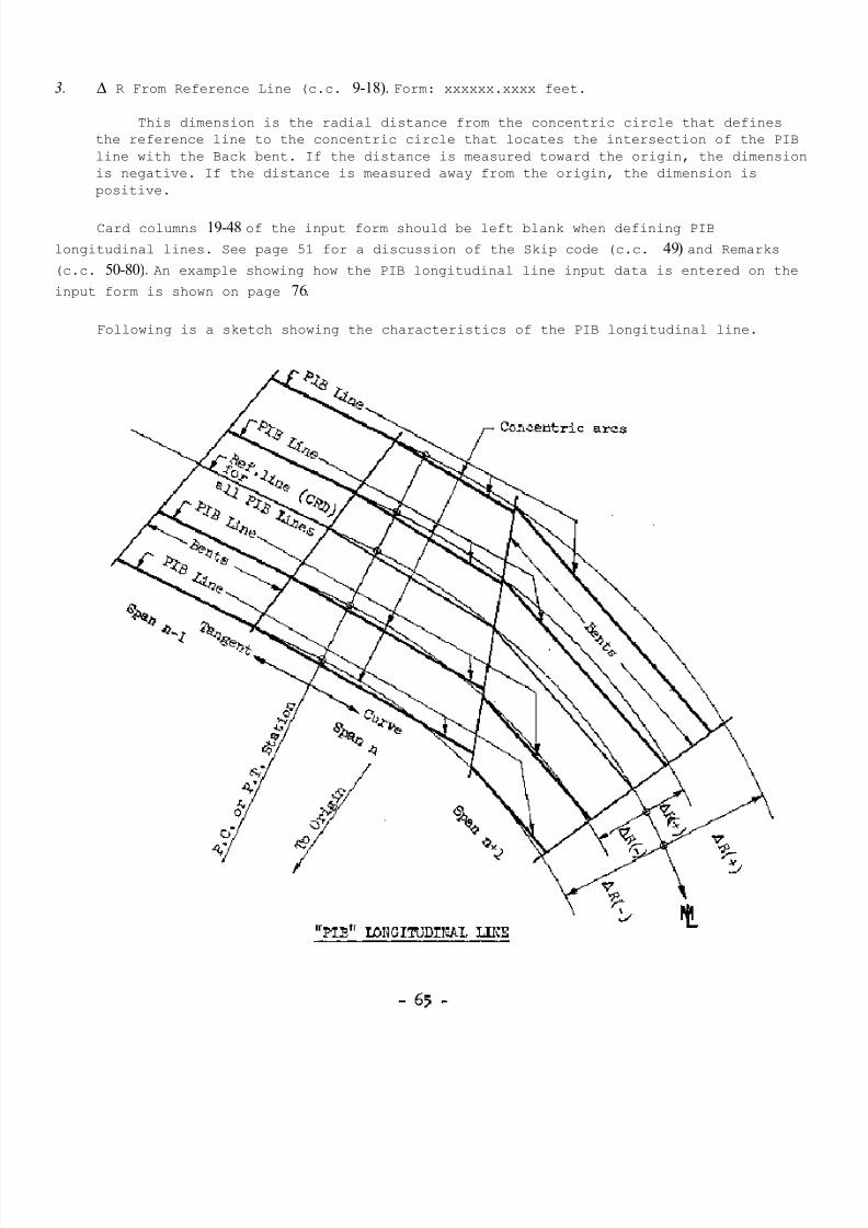
7/21/2019 Georgia Skew
http://slidepdf.com/reader/full/georgia-skew 73/182
3. ∆ R From Reference Line (c.c. 9-18). Form: xxxxxx.xxxx feet.
This dimension is the radial distance from the concentric circle that defines
the reference line to the concentric circle that locates the intersection of the PIB
line with the Back bent. If the distance is measured toward the origin, the dimension
is negative. If the distance is measured away from the origin, the dimension is
positive.
Card columns 19-48 of the input form should be left blank when defining PIB
longitudinal lines. See page 51 for a discussion of the Skip code (c.c. 49) and Remarks
(c.c. 50-80). An example showing how the PIB longitudinal line input data is entered on the
input form is shown on page 76.
Following is a sketch showing the characteristics of the PIB longitudinal line.
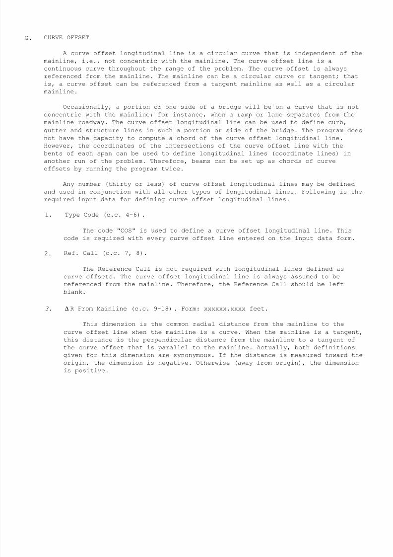
7/21/2019 Georgia Skew
http://slidepdf.com/reader/full/georgia-skew 74/182
G. CURVE OFFSET
A curve offset longitudinal line is a circular curve that is independent of the
mainline, i.e., not concentric with the mainline. The curve offset line is a
continuous curve throughout the range of the problem. The curve offset is always
referenced from the mainline. The mainline can be a circular curve or tangent; that
is, a curve offset can be referenced from a tangent mainline as well as a circular
mainline.
Occasionally, a portion or one side of a bridge will be on a curve that is not
concentric with the mainline; for instance, when a ramp or lane separates from the
mainline roadway. The curve offset longitudinal line can be used to define curb,
gutter and structure lines in such a portion or side of the bridge. The program does
not have the capacity to compute a chord of the curve offset longitudinal line.
However, the coordinates of the intersections of the curve offset line with the
bents of each span can be used to define longitudinal lines (coordinate lines) in
another run of the problem. Therefore, beams can be set up as chords of curve
offsets by running the program twice.
Any number (thirty or less) of curve offset longitudinal lines may be defined
and used in conjunction with all other types of longitudinal lines. Following is the
required input data for defining curve offset longitudinal lines.
1. Type Code (c.c. 4-6).
The code "COS" is used to define a curve offset longitudinal line. This
code is required with every curve offset line entered on the input data form.
2. Ref. Call (c.c. 7, 8).
The Reference Call is not required with longitudinal lines defined as
curve offsets. The curve offset longitudinal line is always assumed to be
referenced from the mainline. Therefore, the Reference Call should be left
blank.
3. ∆ R From Mainline (c.c. 9-18). Form: xxxxxx.xxxx feet.
This dimension is the common radial distance from the mainline to the
curve offset line when the mainline is a curve. When the mainline is a tangent,
this distance is the perpendicular distance from the mainline to a tangent of
the curve offset that is parallel to the mainline. Actually, both definitions
given for this dimension are synonymous. If the distance is measured toward the
origin, the dimension is negative. Otherwise (away from origin), the dimension
is positive.
7/21/2019 Georgia Skew
http://slidepdf.com/reader/full/georgia-skew 75/182
4. Mainline Control Station (c.c. 19-28). Form: xxxx+xx.xxxx feet.
The Control Station is the mainline station of the point where the "D R From
Mainline" dimension is given. This station is always required when defining curve
offset longitudinal lines. The Control Station may be of negative magnitude, and this
station is completely independent of any other station given in the input data. Note
that this station must be a mainline station and not a station along the curve offset
line. A tangent to the curve offset line at the Control Station will be parallel to a
tangent of the mainline curve at the Control Station.
5. Radius (c.c. 29-38). Form: xxxxxx.xxxx feet.
Enter in this column the radius of the curve offset longitudinal line. This
dimension should always be given, and it is required that this dimension be greater
than zero.
Card columns 39-48 of the input form should be left blank when defining a curve
offset longitudinal line. The Skip code (c.c. 49) and Remarks (c.c. 50-80) are discussed
on page 51. An example showing how the curve offset longitudinal line data is entered on
the input form is shown on page 78.
Following is a sketch showing the characteristics of the curve offset longitudinal
line.
7/21/2019 Georgia Skew
http://slidepdf.com/reader/full/georgia-skew 76/182
H. STRAIGHT TAPER
A straight taper is defined as a line whose distance from the mainline varies
lineally. If the main line is a circular curve, the straight taper varies lineally
from a tangent to the mainline curve. Therefore, the straight taper longitudinal line
will always be a straight line that is continuous throughout the range of the bridge
and which is completely independent of a change in the mainline from tangent to curve
or vice versa.
Occasionally, one side of a bridge will be on a straight taper from the
mainline, i.e., the beginning of a new lane or ramp, etc. The straight taper
longitudinal line can be used to represent the curb, gutter and structure lines in
this case. In addition, straight taper lines may be used to enter splayed beams,
i.e., non-parallel beams.
A special case of straight taper line usage is when the rate of taper is set
equal to zero. In this case, the straight taper is parallel to the main line. For an
example, lets assume a four-span bridge where a short portion of one end span is in a
circular curve - the rest of the bridge is on a tangent. It is desired to make this
a continuous unit and extend the beams straight into the curve portion. The beams can
be set up as straight taper longitudinal lines with a zero taper rate. No other type
of longitudinal line can be set up for this type of usage except the coordinate
longitudinal line. However, the coordinates would have to be computed to define a
coordinate line making this alternate somewhat cumbersome.
Any number (thirty or less) of straight taper longitudinal lines may be defined
and used in conjunction with all other types of longitudinal lines. Following is the
required input data for defining straight taper longitudinal lines.
1. Type Code (c.c. 4-6).
The code "STP" is used to define a straight taper longitudinal line. This
code is required with every straight taper line entered on the input data form.
2. Ref. Call (c.c. 7, 8).
The Reference Call is not required with longitudinal lines defined as
straight tapers. Since the straight taper line is always referenced from the
main line, the Reference Call should be left blank.
3. &R From Mainline (c.c. 9-18). Form: xxxxxx.xxxx feet.
This dimension is the distance from the mainline to a point on the
straight taper line and is measured normal (perpendicular) to the mainline (or
mainline tangent). If the distance is measured toward the origin, the dimension
is negative; otherwise, the dimension is positive.
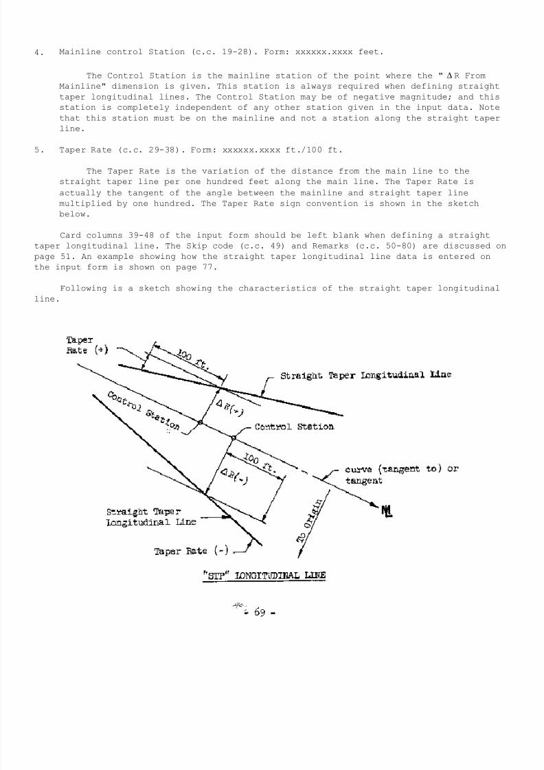
7/21/2019 Georgia Skew
http://slidepdf.com/reader/full/georgia-skew 77/182
4. Mainline control Station (c.c. 19-28). Form: xxxxxx.xxxx feet.
The Control Station is the mainline station of the point where the "∆ R From
Mainline" dimension is given. This station is always required when defining straight
taper longitudinal lines. The Control Station may be of negative magnitude; and this
station is completely independent of any other station given in the input data. Note
that this station must be on the mainline and not a station along the straight taper
line.
5. Taper Rate (c.c. 29-38). Form: xxxxxx.xxxx ft./100 ft.
The Taper Rate is the variation of the distance from the main line to the
straight taper line per one hundred feet along the main line. The Taper Rate is
actually the tangent of the angle between the mainline and straight taper line
multiplied by one hundred. The Taper Rate sign convention is shown in the sketch
below.
Card columns 39-48 of the input form should be left blank when defining a straight
taper longitudinal line. The Skip code (c.c. 49) and Remarks (c.c. 50-80) are discussed on
page 51. An example showing how the straight taper longitudinal line data is entered on
the input form is shown on page 77.
Following is a sketch showing the characteristics of the straight taper longitudinal
line.
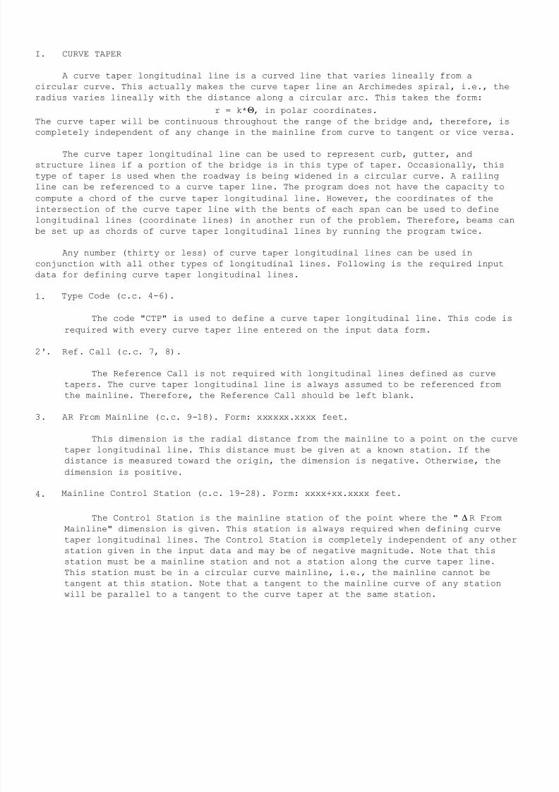
7/21/2019 Georgia Skew
http://slidepdf.com/reader/full/georgia-skew 78/182
I. CURVE TAPER
A curve taper longitudinal line is a curved line that varies lineally from a
circular curve. This actually makes the curve taper line an Archimedes spiral, i.e., the
radius varies lineally with the distance along a circular arc. This takes the form:
r = k*Θ, in polar coordinates.
The curve taper will be continuous throughout the range of the bridge and, therefore, is
completely independent of any change in the mainline from curve to tangent or vice versa.
The curve taper longitudinal line can be used to represent curb, gutter, and
structure lines if a portion of the bridge is in this type of taper. Occasionally, this
type of taper is used when the roadway is being widened in a circular curve. A railing
line can be referenced to a curve taper line. The program does not have the capacity to
compute a chord of the curve taper longitudinal line. However, the coordinates of the
intersection of the curve taper line with the bents of each span can be used to define
longitudinal lines (coordinate lines) in another run of the problem. Therefore, beams can
be set up as chords of curve taper longitudinal lines by running the program twice.
Any number (thirty or less) of curve taper longitudinal lines can be used in
conjunction with all other types of longitudinal lines. Following is the required input
data for defining curve taper longitudinal lines.
1. Type Code (c.c. 4-6).
The code "CTP" is used to define a curve taper longitudinal line. This code is
required with every curve taper line entered on the input data form.
2'. Ref. Call (c.c. 7, 8).
The Reference Call is not required with longitudinal lines defined as curve
tapers. The curve taper longitudinal line is always assumed to be referenced from
the mainline. Therefore, the Reference Call should be left blank.
3. AR From Mainline (c.c. 9-18). Form: xxxxxx.xxxx feet.
This dimension is the radial distance from the mainline to a point on the curve
taper longitudinal line. This distance must be given at a known station. If the
distance is measured toward the origin, the dimension is negative. Otherwise, the
dimension is positive.
4. Mainline Control Station (c.c. 19-28). Form: xxxx+xx.xxxx feet.
The Control Station is the mainline station of the point where the "∆ R From
Mainline" dimension is given. This station is always required when defining curve
taper longitudinal lines. The Control Station is completely independent of any other
station given in the input data and may be of negative magnitude. Note that this
station must be a mainline station and not a station along the curve taper line.
This station must be in a circular curve mainline, i.e., the mainline cannot be
tangent at this station. Note that a tangent to the mainline curve of any station
will be parallel to a tangent to the curve taper at the same station.
7/21/2019 Georgia Skew
http://slidepdf.com/reader/full/georgia-skew 79/182
5. Taper Rate (c.c. 29-38). Form: xxxxxx.xxxx ft./100 ft.
The Taper Rate is the change in radius of the curve taper longitudinal line per
one hundred feet along the mainline. The Taper Rate must always be defined when
entering curve taper longitudinal lines, i.e., cannot be left blank or given a value
of zero. If the radius of the curve taper line increases as the stations increase,
the taper rate is positive. If the radius of the curve taper line decreases as the
stations increase, the taper rate is negative.
Card columns 39-48 of the input form should be left blank when defining a curve taper
longitudinal line. The Skip code (c.c. 49) and Remarks (c.c. 50-80) are discussed on page
51. An example showing how the curve taper longitudinal line data is entered on the input
form is shown on page 78.
Following is a sketch showing the characteristics of the curve taper longitudinal
line.
7/21/2019 Georgia Skew
http://slidepdf.com/reader/full/georgia-skew 80/182
J. COORDINATE
A coordinate longitudinal line is a straight line throughout the range of the
bridge and, therefore, is completely independent of the mainline. The coordinate line
is defined by entering the X and Y coordinates of two points on the coordinate line.
The coordinates are assumed or computed by hand or another program. Note that this
program can be used to compute coordinates that can be used to define coordinate
longitudinal lines in subsequent runs of the problem.
This type of longitudinal line can be used to represent most any kind of
straight line on the bridge provided, of course, the coordinates are known, i.e.,
curbs, gutter, beam and structure lines.
Any number (thirty or less) of coordinate longitudinal lines may be defined and
used in conjunction with all other types of longitudinal lines. Following is the
required input data for defining coordinate longitudinal lines.
I. Type Code (c.c. 4-6).
The code "COR" is used to define a coordinate longitudinal line. This code
is required with every coordinate line entered on the input data form.
2. Ref. Call (c.c. 7, 8).
The Reference Call is not required with longitudinal lines defined as
coordinate lines. Therefore, the Ref. Call should be left blank.
3. Coordinates (c.c. 9-48). Form: xxxxxx.xxxx feet.
Note that the input form has a separate heading (format) for use when
entering a coordinate defined longitudinal line. The X-coordinate of point one
is entered in c.c. 9-18, and the Y-coordinate of point one is entered in c.c.
19-28. The X-coordinate of point two is entered in c.c. 29-38, and the Y-
coordinate of point two is entered in c.c. 39-48.
The Skip code (c.c. 49) and Remarks are discussed on page 51. An example
showing how the coordinate longitudinal line data is entered on the input form is
shown on page 77.
On the following page is a sketch showing the characteristics of the coordinate
longitudinal line.
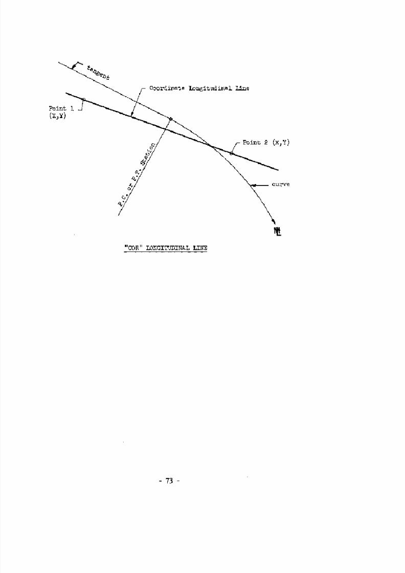
7/21/2019 Georgia Skew
http://slidepdf.com/reader/full/georgia-skew 81/182
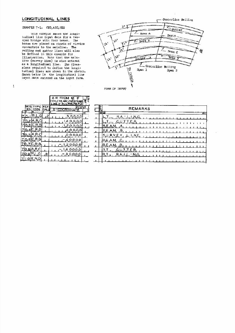
7/21/2019 Georgia Skew
http://slidepdf.com/reader/full/georgia-skew 82/182
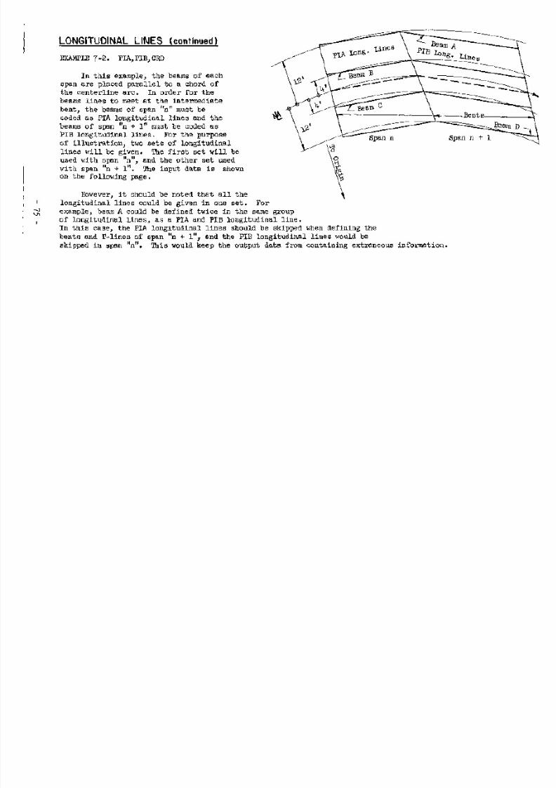
7/21/2019 Georgia Skew
http://slidepdf.com/reader/full/georgia-skew 83/182
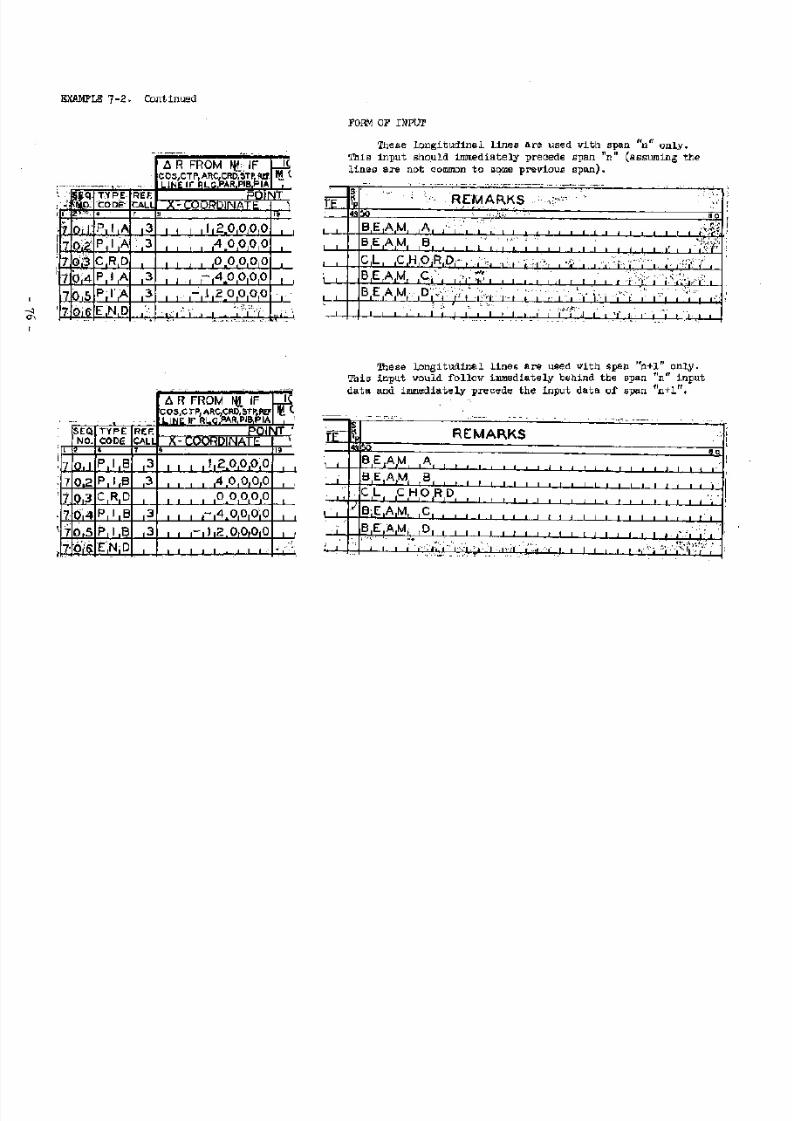
7/21/2019 Georgia Skew
http://slidepdf.com/reader/full/georgia-skew 84/182
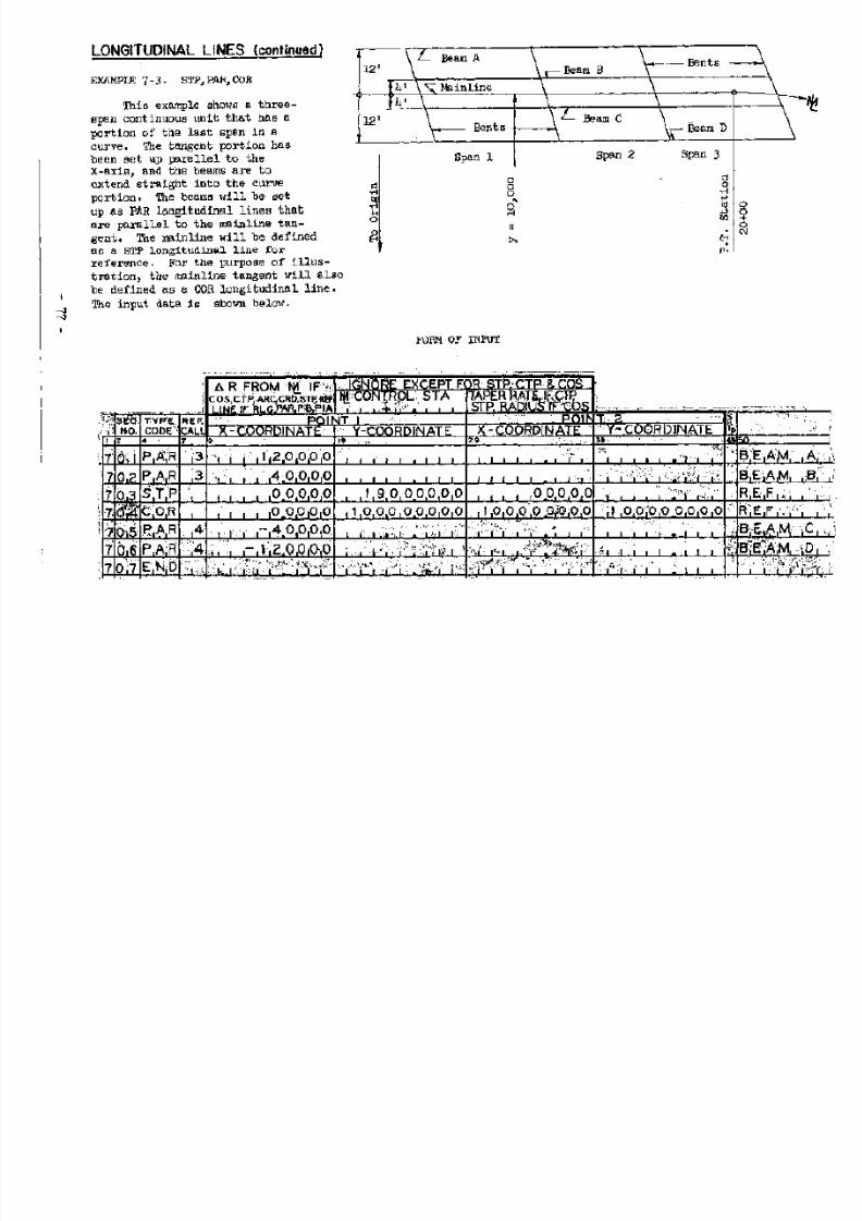
7/21/2019 Georgia Skew
http://slidepdf.com/reader/full/georgia-skew 85/182
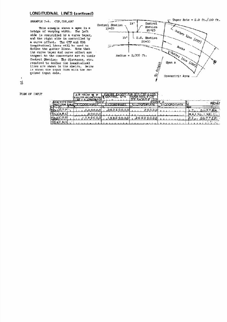
7/21/2019 Georgia Skew
http://slidepdf.com/reader/full/georgia-skew 86/182
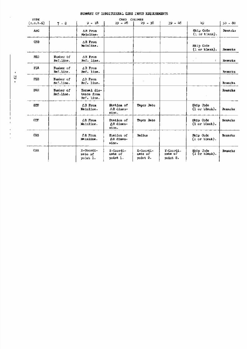
7/21/2019 Georgia Skew
http://slidepdf.com/reader/full/georgia-skew 87/182
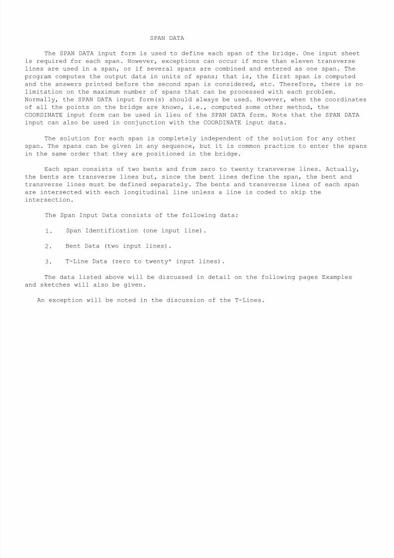
7/21/2019 Georgia Skew
http://slidepdf.com/reader/full/georgia-skew 88/182
SPAN DATA
The SPAN DATA input form is used to define each span of the bridge. One input sheet
is required for each span. However, exceptions can occur if more than eleven transverse
lines are used in a span, or if several spans are combined and entered as one span. The
program computes the output data in units of spans; that is, the first span is computed
and the answers printed before the second span is considered, etc. Therefore, there is no
limitation on the maximum number of spans that can be processed with each problem.
Normally, the SPAN DATA input form(s) should always be used. However, when the coordinates
of all the points on the bridge are known, i.e., computed some other method, the
COORDINATE input form can be used in lieu of the SPAN DATA form. Note that the SPAN DATA
input can also be used in conjunction with the COORDINATE input data.
The solution for each span is completely independent of the solution for any other
span. The spans can be given in any sequence, but it is common practice to enter the spans
in the same order that they are positioned in the bridge.
Each span consists of two bents and from zero to twenty transverse lines. Actually,
the bents are transverse lines but, since the bent lines define the span, the bent and
transverse lines must be defined separately. The bents and transverse lines of each span
are intersected with each longitudinal line unless a line is coded to skip the
intersection.
The Span Input Data consists of the following data:
1. Span Identification (one input line).
2. Bent Data (two input lines).
3. T-Line Data (zero to twenty* input lines).
The data listed above will be discussed in detail on the following pages Examples
and sketches will also be given.
An exception will be noted in the discussion of the T-Lines.
7/21/2019 Georgia Skew
http://slidepdf.com/reader/full/georgia-skew 89/182
A. Span Identification (8 SPAN in c.c. 1-5).
The Span Identification consists of data pertinent to the processing of the
span and Remarks that identify the span. The Span Identification data is entered on
one line of the input form, and this line is the first input line of the SPAN DATA
input form. The Span Identification should always contain data except as noted on
page 95. An example of the Span Identification input is not given since it is felt
that the instructions are adequate. Following are the input data requirements.
1. Span Number (c.c. 7, 8). Form: xx
Enter in this space the span number. Either numbers or characters may be
used, i.e., 1, 2, 3L, 4R, etc. This number will be given in the output data of
the span. There is no sequence check on the order of the Span Numbers.
2. Number of Transverse Lines (c.c. 10, 11). Form: xx
The Number of Transverse Lines that are going to be defined in the span
should be given in this space. If no T-lines are going to be defined, this
number may be left blank or given a value of zero. Since the maximum number of
T-lines is twenty per span, this number cannot exceed twenty. Therefore, the
Number of Transverse Lines will vary from zero (0) to twenty (20). Note that
this number is the total number of T-lines in the span and not, necessarily,
the number of T-lines defined on one SPAN DATA input form, i.e., two sheets can
be used when more than eleven T-lines are defined.
3. Last Span Code (c.c. 13-16).
The code "LAST" should be entered in this space when filling in the input
data of the last span of the problem. This space should be left blank in all
preceding spans. This code indicates to the program that no further input data
is going to be given after the present (last) span. Whenever coordinates are
used as input data (on COORDINATE input data form) after the last span,, the
Last Span Code should be left blank since additional input data must beprocessed.
4. Remarks (c.c. 16-73).
This space is provided so that the Engineer can enter any pertinent
Remarks describing the span. These Remarks will appear in the output data of
the span.
5. Code for Additional Longitudinal Lines (c-c. 74-76).
Whenever another set of longitudinal lines are going to be defined
immediately after a SPAN DATA input sheet, the code "YES" should be given in
card columns 74-76 of the Span Identification. Otherwise, these card columnscan be used for Remarks. Therefore, if "YES" is given in these card columns,
the program will expect the next sheet of input data after the span input data
to be LONGITUDINAL LINES.
7/21/2019 Georgia Skew
http://slidepdf.com/reader/full/georgia-skew 90/182
B. Bent Data (B or A in c.c. 1).
Two lines on the SPAN DATA input form are provided so that the two bents that
define each span can be defined. The bent that begins the span will be referred to as
the Back bent and should always be defined first, i.e., on the input line with the
letter "B" in card column one. The bent that terminates the span will be referred to
as the Ahead bent and should always be defined next on the input line with the letter
"A" in card column one. The Back and Ahead bent must always be given when defining a
span. Note that a bent common to two spans must be defined twice, once with each
span.
Except as noted otherwise, the procedure for defining the Back and Ahead bent
is identical. Following is the input data required to define the bents.
1. RLG Intersect Code (c.c. 2).
This code is used to indicate to the program which point of intersection the
program is to consider when intersecting the bent line with the railing longitudinal
lines of the span. If the bent line is to extend straight and intersect the railing
lines, the digit one (1) should be entered as the RLG Intersect Code. However, if the
bent line is to turn at the intersection of the bent line with the reference line of
the railing line and extend radially from the reference line to intersect the railing
longitudinal line, the RLG Intersect Code should be left blank or given a value of
zero. Note that the bent line will intersect all railing longitudinal lines in the
same fashion. A sketch showing this optional point of intersection is shown on page
58. This code has no effect on the intersection of the bent line with other types of
longitudinal lines, nor on any longitudinal lines located between the railing line
and its reference line.
2. Bent Number (c.c. 3, 4). Form: xx.
This space is for entering the number of the bent. This number can be
numeric or alphabetic characters and will appear in the output data.
3. Remarks (c.c. 37-50).
This space is provided so that the user can enter any pertinent Remarks
that describe the bent. These Remarks will appear in the output data to assist
in the interpretation of the output.
4. Longitudinal Line Skips (c.c. 51-80).
The longitudinal Line Skip is used to instruct the program to by-pass the
intersection of the bent line with some particular longitudinal line. The digit
one (1) is used to indicate that the intersection is to be skipped. Otherwise.,
the Longitudinal Line Skip is left blank. For example, if the intersection of
the bent with longitudinal line four (4) is not desired in the output data, thedigit "I" should be entered in card column 54. Note that immediately below the
Longitudinal Line Skip heading there are numbers that correspond to the
longitudinal line number (1-30), and immediately below the longitudinal line
numbers are the card column numbers (51-8o).
It is important to note that if the Longitudinal Line Skip is coded to skip a
longitudinal line when defining the Ahead bent, the length of that longitudinal line
from the Back bent to the Ahead bent will not be given in the output data. Also, when
a bent is coded to skip a longitudinal line, the "Distance to Previous Point"
7/21/2019 Georgia Skew
http://slidepdf.com/reader/full/georgia-skew 91/182
dimension given in the output data will be zero in the output data of the
intersection of the bent with the next longitudinal line. For example, the distance
from the point of intersection of the bent with longitudinal line "n-l" to the point
of intersection of the bent with longitudinal line "n+l" is not given in the output
data when longitudinal line "n" is skipped. If a longitudinal line has been coded to
skip all intersections (the digit one entered in card column 49 of the longitudinal
Line input data) the bent Longitudinal Line Skip for that longitudinal line is
meaningless, since the bent will not be intersected with the longitudinal in any
event.
5. Type Code (c.c. 5-8).
The Type Code is used to indicate to the program how the bent is going to be
defined. There are five codes available to the Engineer with which the bent can be
defined. They are:
1) SKEW (Skewed at a station)
2) PARL (Parallel to reference line at a normal distance)
3) PSTA (Parallel to reference line at a station)
4) PREV (Parallel to bent B at a normal distance or a station)
5) SAME (Same as bent A of preceding span)
It is left up to the user to select the code and data that can most conveniently be
used to define the bent. Following is a discussion and sketch of each Type Code, the
required input data of each type, and examples (pages 90-92) showing how the data is
entered on the input data form.
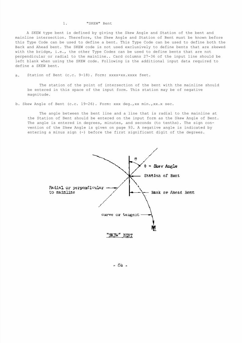
7/21/2019 Georgia Skew
http://slidepdf.com/reader/full/georgia-skew 92/182
1. "SKEW" Bent
A SKEW type bent is defined by giving the Skew Angle and Station of the bent and
mainline intersection. Therefore, the Skew Angle and Station of Bent must be known before
this Type Code can be used to define a bent. This Type Code can be used to define both the
Back and Ahead bent. The SKEW code is not used exclusively to define bents that are skewed
with the bridge, i.e., the other Type Codes can be used to define bents that are not
perpendicular or radial to the mainline.. Card columns 27-36 of the input line should be
left blank when using the SKEW code. Following is the additional input data required to
define a SKEW bent.
a. Station of Bent (c.c. 9-18). Form: xxxx+xx.xxxx feet.
The station of the point of intersection of the bent with the mainline should
be entered in this space of the input form. This station may be of negative
magnitude.
b. Skew Angle of Bent (c.c. 19-26). Form: xxx deg.,xx min.,xx.x sec.
The angle between the bent line and a line that is radial to the mainline at
the Station of Bent should be entered on the input form as the Skew Angle of Bent.
The angle is entered in degrees, minutes, and seconds (to tenths). The sign con-
vention of the Skew Angle is given on page 93. A negative angle is indicated by
entering a minus sign (-) before the first significant digit of the degrees.
7/21/2019 Georgia Skew
http://slidepdf.com/reader/full/georgia-skew 93/182
2. "PARL" Bent
A PARL type bent is defined by first defining a reference line. The bent is defined
to be parallel to this reference line at a given normal distance from the reference line.
The reference line can be another bent or any arbitrary line; however, the skew angle and
mainline station of the reference line must be known. The reference line will not be
intersected with any of the longitudinal lines. The Back and Ahead bent may be defined by
this Type Code. Following is the additional input data required to define a PARL bent.
a. Station of Reference Line (c.c. 9-18). Form: xxxx+xx.xxxx feet.
Enter in this space the station of the intersection of the reference line with
the mainline. This station may be of negative magnitude.
b. Skew Angle of Reference Line (c.c. 19-26).
Form: xxx deg.,xx min.,xx.x sec.
The angle between the reference line and a line radial to the mainline at the
Station of Reference Line should be entered on the input form as the Skew Angle of
Reference Line. The angle is entered in degrees, minutes, and seconds (to tenths).
See page 93 for the Skew Angle sign convention. A negative angle is indicated by
placing a minus sign (-) before the first significant digit of the degrees.
C. Normal Distance (c.c. 27-36). Form: xxxxxx.xxxx feet.
Enter in this space the Normal Distance from the reference line to the bent
line. If the bent is ahead of the reference line ' the distance is positive.
Otherwise (bent back of the reference line), the distance is negative.
"PARL" Bent
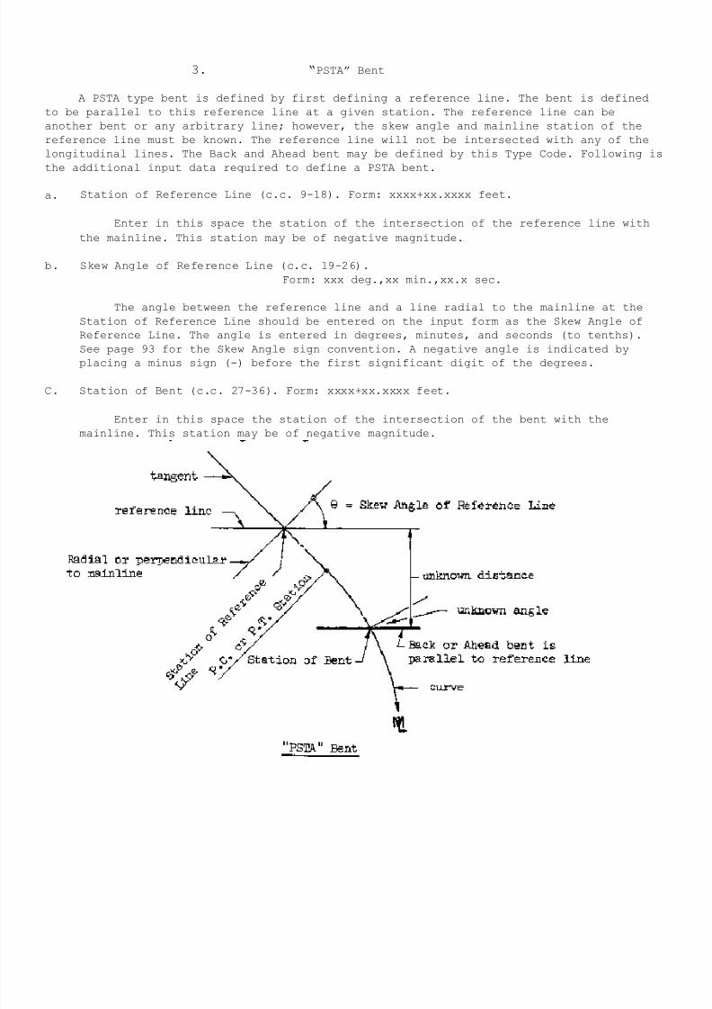
7/21/2019 Georgia Skew
http://slidepdf.com/reader/full/georgia-skew 94/182
3. “PSTA” Bent
A PSTA type bent is defined by first defining a reference line. The bent is defined
to be parallel to this reference line at a given station. The reference line can be
another bent or any arbitrary line; however, the skew angle and mainline station of the
reference line must be known. The reference line will not be intersected with any of the
longitudinal lines. The Back and Ahead bent may be defined by this Type Code. Following is
the additional input data required to define a PSTA bent.
a. Station of Reference Line (c.c. 9-18). Form: xxxx+xx.xxxx feet.
Enter in this space the station of the intersection of the reference line with
the mainline. This station may be of negative magnitude.
b. Skew Angle of Reference Line (c.c. 19-26).
Form: xxx deg.,xx min.,xx.x sec.
The angle between the reference line and a line radial to the mainline at the
Station of Reference Line should be entered on the input form as the Skew Angle of
Reference Line. The angle is entered in degrees, minutes, and seconds (to tenths).
See page 93 for the Skew Angle sign convention. A negative angle is indicated byplacing a minus sign (-) before the first significant digit of the degrees.
C. Station of Bent (c.c. 27-36). Form: xxxx+xx.xxxx feet.
Enter in this space the station of the intersection of the bent with the
mainline. This station may be of negative magnitude.
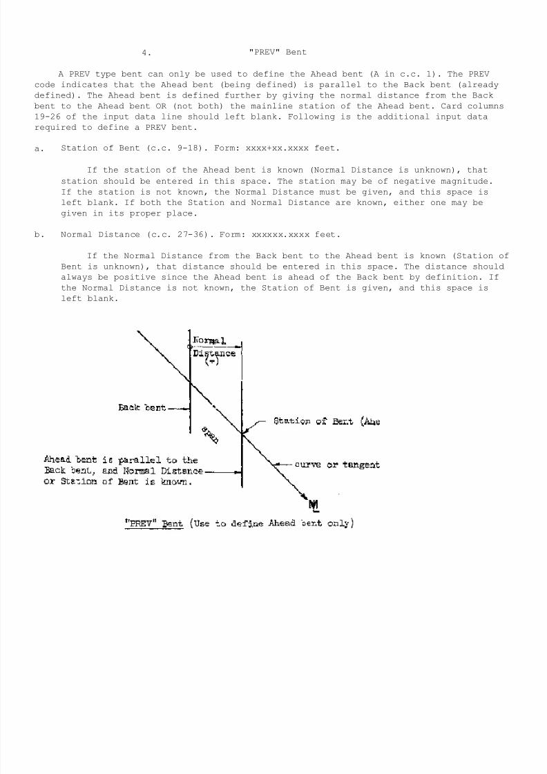
7/21/2019 Georgia Skew
http://slidepdf.com/reader/full/georgia-skew 95/182
4. "PREV" Bent
A PREV type bent can only be used to define the Ahead bent (A in c.c. 1). The PREV
code indicates that the Ahead bent (being defined) is parallel to the Back bent (already
defined). The Ahead bent is defined further by giving the normal distance from the Back
bent to the Ahead bent OR (not both) the mainline station of the Ahead bent. Card columns
19-26 of the input data line should left blank. Following is the additional input data
required to define a PREV bent.
a. Station of Bent (c.c. 9-18). Form: xxxx+xx.xxxx feet.
If the station of the Ahead bent is known (Normal Distance is unknown), that
station should be entered in this space. The station may be of negative magnitude.
If the station is not known, the Normal Distance must be given, and this space is
left blank. If both the Station and Normal Distance are known, either one may be
given in its proper place.
b. Normal Distance (c.c. 27-36). Form: xxxxxx.xxxx feet.
If the Normal Distance from the Back bent to the Ahead bent is known (Station of
Bent is unknown), that distance should be entered in this space. The distance should
always be positive since the Ahead bent is ahead of the Back bent by definition. If
the Normal Distance is not known, the Station of Bent is given, and this space is
left blank.
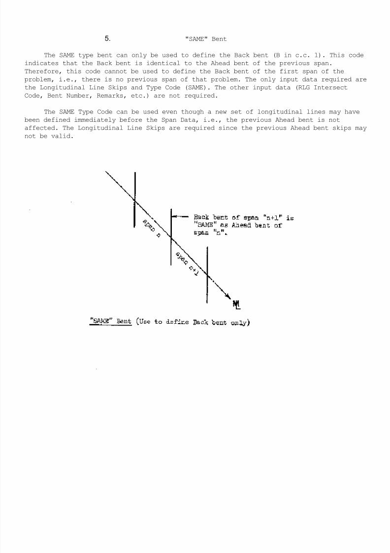
7/21/2019 Georgia Skew
http://slidepdf.com/reader/full/georgia-skew 96/182
5. "SAME" Bent
The SAME type bent can only be used to define the Back bent (B in c.c. 1). This code
indicates that the Back bent is identical to the Ahead bent of the previous span.
Therefore, this code cannot be used to define the Back bent of the first span of the
problem, i.e., there is no previous span of that problem. The only input data required are
the Longitudinal Line Skips and Type Code (SAME). The other input data (RLG Intersect
Code, Bent Number, Remarks, etc.) are not required.
The SAME Type Code can be used even though a new set of longitudinal lines may have
been defined immediately before the Span Data, i.e., the previous Ahead bent is not
affected. The Longitudinal Line Skips are required since the previous Ahead bent skips may
not be valid.
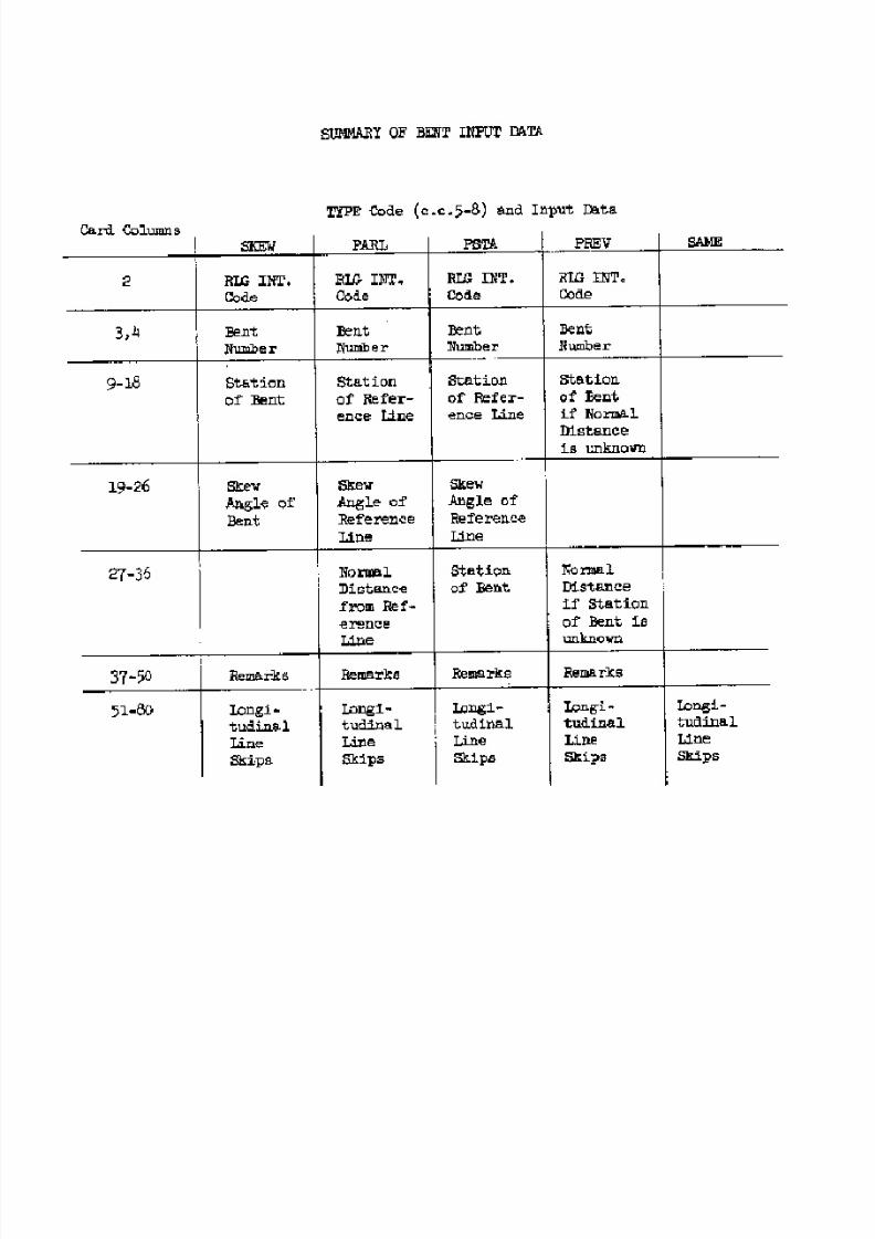
7/21/2019 Georgia Skew
http://slidepdf.com/reader/full/georgia-skew 97/182
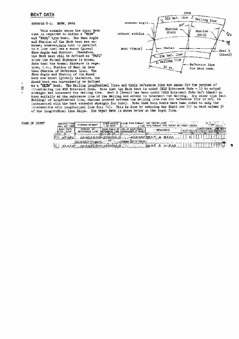
7/21/2019 Georgia Skew
http://slidepdf.com/reader/full/georgia-skew 98/182
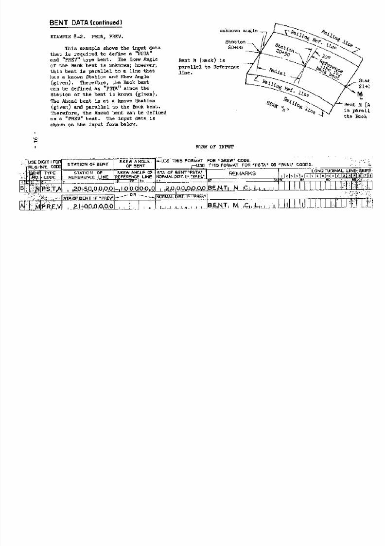
7/21/2019 Georgia Skew
http://slidepdf.com/reader/full/georgia-skew 99/182
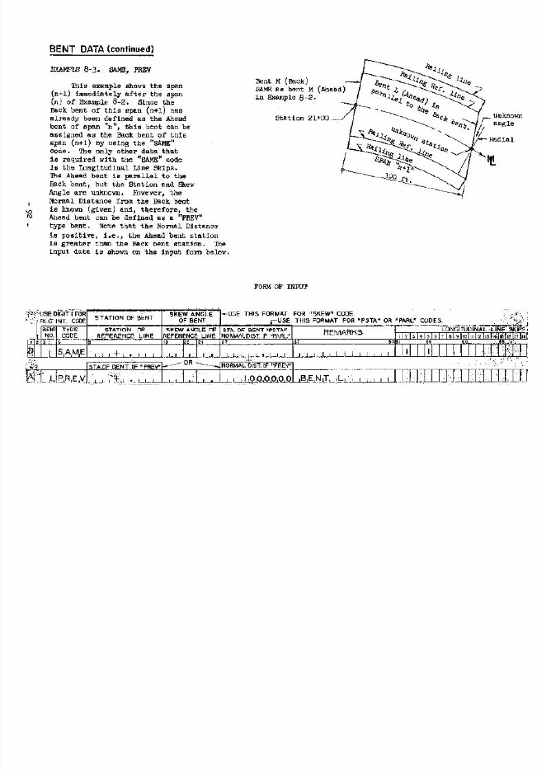
7/21/2019 Georgia Skew
http://slidepdf.com/reader/full/georgia-skew 100/182
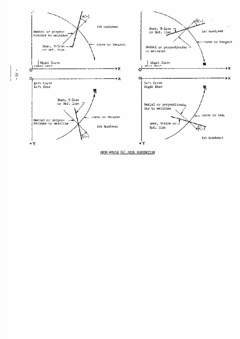
7/21/2019 Georgia Skew
http://slidepdf.com/reader/full/georgia-skew 101/182
7/21/2019 Georgia Skew
http://slidepdf.com/reader/full/georgia-skew 102/182
C. Transverse Lines (T-Lines).
Transverse lines are lines that normally run across the bridge and are not
classified as bent lines. The program has the capacity for twenty such lines per
span. T-Lines usually lie between the Ahead and Back bent. However, this is not a
program requirement since the T-Lines are allowed to be outside the range of the
span. Each T-Line along with the Ahead and Back bent will be intersected with each
longitudinal line and the various data of each intersection point given in the
output. T-Lines can be used to represent most any type of transverse line. Following
is a list that shows several examples of T-Line usage, and the purpose for each
usage.
1. Centerline of bearings
The finished grade elevations (output) at the centerline of bearings can
be used for substructure elevations when adjusted for slab, beam depth, etc.
During construction, these elevations can be used to check the top of beam
elevation for any adjustment in the coping depth.
2. Diaphragms
The length, distance from bent, and angle between the diaphragm and
various longitudinal lines, which are given in the output, can be used for
detailing purposes.
3. Substructure lines
Other substructure lines can be used to compute elevations in order to
obtain the substructure elevations, i.e., face of substructure cap. The face of
the substructure cap in the case of the end bent can be used in many instances
to assist in computing railing post spacings.
4. Construction joints
The finished grade elevations at the construction joints can be used by
the field Engineer during construction to set screed elevations.
5. Splice points of beams
The finished grade elevations at the splice points can be used to
determine beam slopes. This is particularly true if a continuous unit is used in
a vertical curve or transition superelevation.
6. Span division lines
The span can be arbitrarily divided by lines in order to compute elevations
for construction purposes, i.e., quarter points, third points, tenth points,etc.
7. Road underneath lines
The edge of paving, shoulder, etc. of the road underneath can be entered as
a T-Line of the bridge above in order to assist in computing clearances.
7/21/2019 Georgia Skew
http://slidepdf.com/reader/full/georgia-skew 103/182
The list of T-Line usage given on the preceding page is by no means a complete list.
However, the lines listed are probably used most often, and they are listed for the
purpose of illustrating how and why T-Lines are used.
The input data necessary to define each T-Line is entered on one line of the input
form (an exception will be noted later). The SPAN DATA input form provides eleven input
data lines for entering the T-Lines. If more than eleven T-Lines are going to be entered
in any one span, additional lines can be attached to the bottom of the input form, or an
additional SPAN DATA input form can be used to enter the additional T-Lines. However, when
an additional input form is used, the Span Identification and Bent Data should be left
blank on the second SPAN DATA input form of the span since a new span is not being
defined, i.e., used solely to enter T-Lines. Note that when using an additional sheet for
T-Lines, or attaching T-Lines to the bottom of the SPAN DATA input form, the Line Number
(c.c. 2, 3) which is given on the input form will have to be changed so that two T-Lines
will not have the same number, i.e., T-Lines must be defined in numerical sequence.
The letter "T" is required in card column one of each T-Line input data line. This
is used by the program for identification purposes. A Line Number is required in card
columns 2 and 3 of the input data lines. This number is assigned to the T-Line and will be
associated with the output data of the T-Line. When more than eleven T-Lines are used per
span, make sure that the letter "T" and the appropriate Line Number are entered on the
additional T-Line input data lines. Note that the letter "T" and Line Number have already
been entered on eleven lines of the input form. Following is the input data common to all
types of T-Lines.
1. RLG Intersect Code (c.c. 36).
The RLG Intersect Code for the T-Line functions in the same manner as the RLG
Intersect Code for the bent lines. See the discussion on page 82 and the sketch on
page 58. Note that the intersecting of a T-Line and any type of longitudinal other
than a railing longitudinal line is found by extending the T-Line straight
regardless of the position of that longitudinal line. When defining a "CONS" First
Code T-Line, the RLG Intersect Code has no meaning and should be left blank.
2. Remarks (c.c. 37-50).
This space is provided so that the user can enter any pertinent Remarks that
describe the T-Line. The Remarks given here will appear in the output data to assist
in the interpretation of the output.
3. Longitudinal Line Skips (c.c. 51-80).
The Longitudinal Line Skips for the T-Lines function in the same manner as the
Longitudinal Line Skips for the bent lines. See the discussion on page 82. Note that
when an intersection is skipped, the output will contain no data relating to that
point of intersection.
7/21/2019 Georgia Skew
http://slidepdf.com/reader/full/georgia-skew 104/182
Two codes are used to indicate how the T-Line is going to be defined: First Code and
Second Code. The First Code denotes how the direction or slope of the T-Line is defined,
and the Second Code denotes how the position of the T-Line is going to be defined. There
are five available First Codes. From one to three different Second Codes are available in
conjunction with each First Code. Following is a list of the five First Codes and the
Second Codes that are available with each.
First Code Second Code
1. PARL NORMDIST
PROP
2. ANGL DIST
PROP
3. PTPT DIST
PROP
COOR
4. SKEW STAT
5. CONS DIST
PROP
From the above list, it can be seen that there are eleven possible combinations of
First and Second Codes. For every T-Line that is defined, the user must decide how that
line can be most conveniently defined. That is, what data is available to define the line
and what Codes can best be used with the available data to define the T-Line. The five
available First Codes are discussed in detail on the following pages. The required input
data for each available Second Code is given in the discussion of each T-Line First Code.
Examples of T-Lines defined on the input form are given on pages 110 to 113.
7/21/2019 Georgia Skew
http://slidepdf.com/reader/full/georgia-skew 105/182
1. "PARL" T-Line
The "PARL" First Code defines a straight T-Line that is parallel to either the Ahead
or Back bent. A T-Line cannot be defined as being parallel to any other type of line,
i.e., another T-Line or reference line. A T-Line is designated as parallel to a bent when
the Code "PARL" is entered in card columns 4-7 of the T-Line input data line. The position
of the "PARL" T-Line can be defined by any one of three available options. The option or
method that is used must be indicated by the Second Code. The three Second Codes and the
required input data for each are as follows.
First and Second Code Required Input Data
PARL/NORM Reference Bent, Normal distance
PARL/DIST Reference Bent, Distance, Reference Line
PARI/PROP Reference Bent, Proportion, Reference Line
a. Reference Bent (c.c. 12). A or B
The Reference Bent indicates the bent to which the "PARL" T-Line is parallel.
Therefore, this Reference Bent designation is always required with a "PARL" First
Code, regardless of the Second Code that is used. Enter the letter "A" to indicate
that the "PARL" T-Line is parallel to the Ahead bent, and the letter "B" is used to
orient the "PARL" T-Line parallel to the Back bent. Any other character or number
entered in this card column will cause an Error Message and terminate the processing
of the problem. The program will not assign a bent by default when an invalid
character is found.
b. Normal, Distance, or Proportion (c.c. 13-22).
Form: xxxxxx.xxxx feet or ratio.
The data entered in this space on the input form depends on the Second Code
used with the "PARL" T-Line.
If the Normal distance from the bent to the T-Line is known, the Second Code
can be given as "NORM" and the Normal distance entered in this space on the input
form. The Normal distance can be given in either direction from either bent.
If the Distance, measured along a longitudinal line, from the bent to the T-
Line is known, the Second Code can be given as "DIST" and the Distance entered in
this space on the input form. This Distance can be measured in either direction from
either bent and along any type of longitudinal line (curve or straight).
If the distance from the bent to the T-Line is to be a Proportion of the length
(from the Back bent to the Ahead bent) of the longitudinal line that the distance is
measured along, the Second Code can be given as "PROP" and the Proportion (ratio)entered in this space on the input form. The Proportion distance can be measured in
either direction from either bent and along any type of longitudinal line.
C. Reference Line (c.c. 23, 24). Form: xx
If the Second Code is "DIST" or "PROP", the number of the longitudinal line
that the Distance or Proportion distance is measured along must be entered in this
space. If the Second Code is "NORM", this space should be left blank.
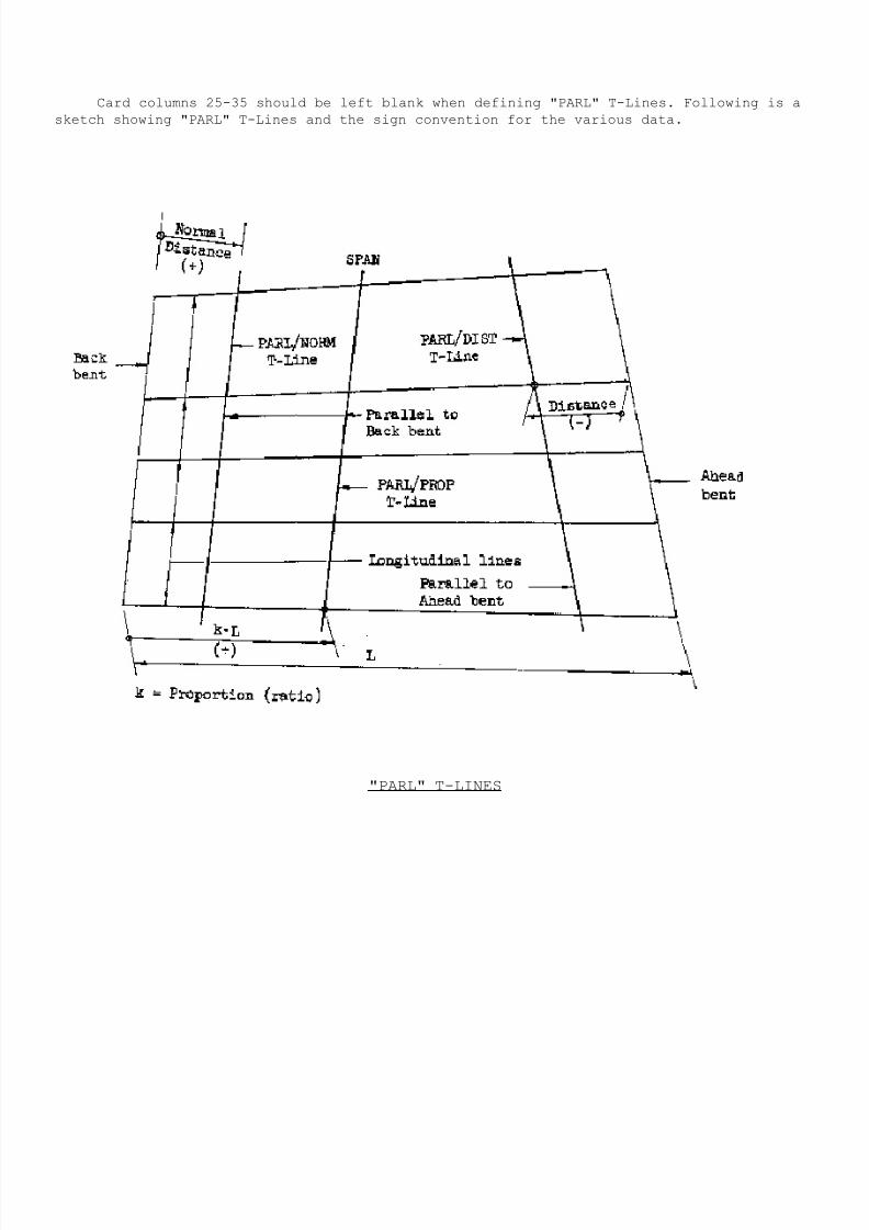
7/21/2019 Georgia Skew
http://slidepdf.com/reader/full/georgia-skew 106/182
Card columns 25-35 should be left blank when defining "PARL" T-Lines. Following is a
sketch showing "PARL" T-Lines and the sign convention for the various data.
"PARL" T-LINES
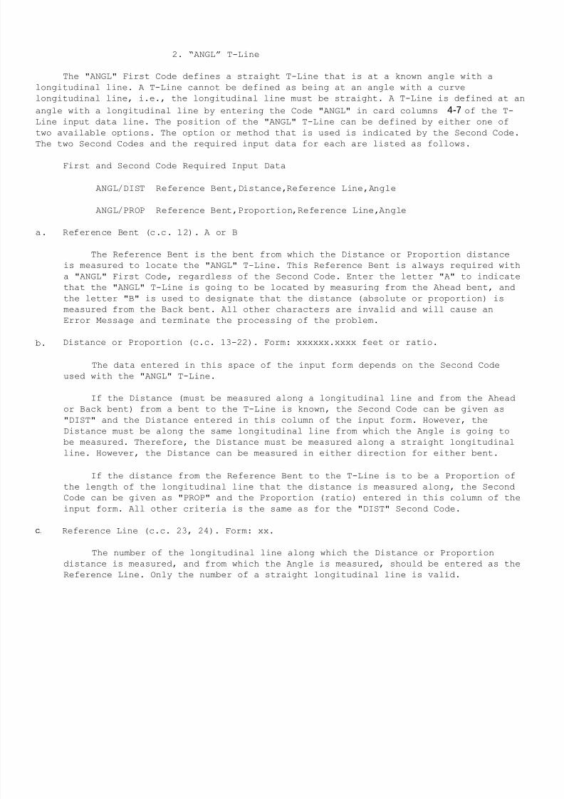
7/21/2019 Georgia Skew
http://slidepdf.com/reader/full/georgia-skew 107/182
2. “ANGL” T-Line
The "ANGL" First Code defines a straight T-Line that is at a known angle with a
longitudinal line. A T-Line cannot be defined as being at an angle with a curve
longitudinal line, i.e., the longitudinal line must be straight. A T-Line is defined at an
angle with a longitudinal line by entering the Code "ANGL" in card columns 4-7 of the T-
Line input data line. The position of the "ANGL" T-Line can be defined by either one of
two available options. The option or method that is used is indicated by the Second Code.
The two Second Codes and the required input data for each are listed as follows.
First and Second Code Required Input Data
ANGL/DIST Reference Bent,Distance,Reference Line,Angle
ANGL/PROP Reference Bent,Proportion,Reference Line,Angle
a. Reference Bent (c.c. 12). A or B
The Reference Bent is the bent from which the Distance or Proportion distance
is measured to locate the "ANGL" T-Line. This Reference Bent is always required with
a "ANGL" First Code, regardless of the Second Code. Enter the letter "A" to indicatethat the "ANGL" T-Line is going to be located by measuring from the Ahead bent, and
the letter "B" is used to designate that the distance (absolute or proportion) is
measured from the Back bent. All other characters are invalid and will cause an
Error Message and terminate the processing of the problem.
b. Distance or Proportion (c.c. 13-22). Form: xxxxxx.xxxx feet or ratio.
The data entered in this space of the input form depends on the Second Code
used with the "ANGL" T-Line.
If the Distance (must be measured along a longitudinal line and from the Ahead
or Back bent) from a bent to the T-Line is known, the Second Code can be given as
"DIST" and the Distance entered in this column of the input form. However, theDistance must be along the same longitudinal line from which the Angle is going to
be measured. Therefore, the Distance must be measured along a straight longitudinal
line. However, the Distance can be measured in either direction for either bent.
If the distance from the Reference Bent to the T-Line is to be a Proportion of
the length of the longitudinal line that the distance is measured along, the Second
Code can be given as "PROP" and the Proportion (ratio) entered in this column of the
input form. All other criteria is the same as for the "DIST" Second Code.
C. Reference Line (c.c. 23, 24). Form: xx.
The number of the longitudinal line along which the Distance or Proportion
distance is measured, and from which the Angle is measured, should be entered as the
Reference Line. Only the number of a straight longitudinal line is valid.
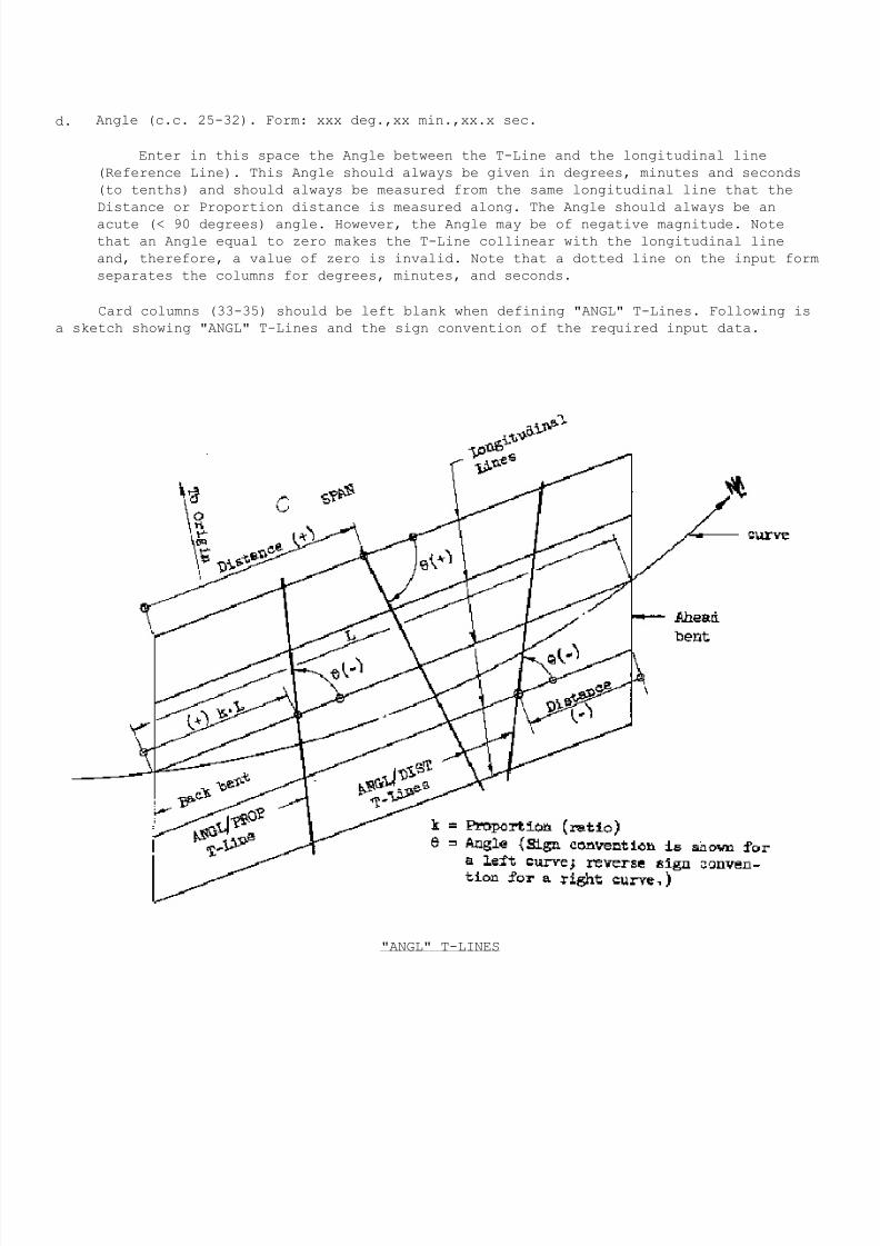
7/21/2019 Georgia Skew
http://slidepdf.com/reader/full/georgia-skew 108/182
d. Angle (c.c. 25-32). Form: xxx deg.,xx min.,xx.x sec.
Enter in this space the Angle between the T-Line and the longitudinal line
(Reference Line). This Angle should always be given in degrees, minutes and seconds
(to tenths) and should always be measured from the same longitudinal line that the
Distance or Proportion distance is measured along. The Angle should always be an
acute (< 90 degrees) angle. However, the Angle may be of negative magnitude. Note
that an Angle equal to zero makes the T-Line collinear with the longitudinal line
and, therefore, a value of zero is invalid. Note that a dotted line on the input form
separates the columns for degrees, minutes, and seconds.
Card columns (33-35) should be left blank when defining "ANGL" T-Lines. Following is
a sketch showing "ANGL" T-Lines and the sign convention of the required input data.
"ANGL" T-LINES
7/21/2019 Georgia Skew
http://slidepdf.com/reader/full/georgia-skew 109/182
3. "PTPT" T-Line
The "PTPT" (Point Point) First Code is used to indicate that the T-Line is going to
be defined by identifying two points on the T-Line, i.e., a straight line between two
points. Such a T-Line is indicated by entering "PTPT" in card columns 4-7 of the T-Line
input data line. The two points, if not defined by coordinates, must be located on the
longitudinal lines. The points that determine the T-Line can be defined by any one of
three available options. The option or method that is used is indicated by the Second
Code. The three Second Codes and the required input data for each type are as follows.
First and Second Code Required Input Data
PTPT/DIST (Point 1) Reference Bent,Distance,Reference Line
(Point 2) Reference Bent,Distance,Reference Line
PTPT/PROP (point 1) Reference Bent,Proportion,Reference Line
(Point 2) Reference Bent,Proportion,Reference Line
PTPT/COOR (Point 1) X-Coordinate, Y-Coordinate
(Point 2) X-Coordinate, Y-Coordinate
a. Reference Bent (c.c. 12 and c.c. 33). A or B
The Reference Bents are the bents from which the Distances or Proportion
distances are measured in order to locate the points that define the T-Line. The
Reference Bents are not required when defining a "COOR" Second Code T-Line since the
input will actually be coordinates, i.e., independent of the Ahead or Back bent.
Each point (except coordinate point) is identified by measuring a Distance or
Proportion distance from the Reference Bent (Back or Ahead bent) along a Reference
Line (longitudinal line). Either point of the T-Line can be located from either
bent. That is, each of the two points that define the "PTPT" T-Line is independent
of the other. "A" is used to indicate that the point is located from the Ahead bent,
and "B" is used to indicate that the point is located from the Back bent. Any
character other than "A" or "B" will cause an Error Message and terminate the
problem. Note that two Reference Bents (one-for each point) must be given. The
Reference Bent (A or B) for point one is given in card column 12, and the ReferenceBent (A or B) for point two is given in card column 33. Which point is designated as
point one, or point two, is arbitrary.
b. Distance, Proportion, or X-Coordinate (c.c. 13-22).
Form: xxxxxx.xxxx feet or ratio.
The data entered in this space of the input form depends on the Second Code
that is used with the "PTPT" T-Line.
If the points that define the T-Line are located by Distances from the
Reference Bents (Ahead or Back) along the Reference Lines (longitudinal lines), the
Second Code should be given as "DIST" and the Distance from the Reference Bent (c.c.
12) to point one given in this column of the input form. The Distance can be
measured from either bent, in either direction, and along any type of longitudinal
line.
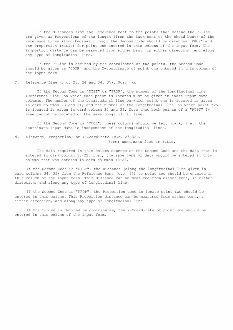
7/21/2019 Georgia Skew
http://slidepdf.com/reader/full/georgia-skew 110/182
If the distances from the Reference Bent to the points that define the T-Line
are given as Proportions of the length (from the Back bent to the Ahead bent) of the
Reference Lines (longitudinal lines), the Second Code should be given as "PROP" and
the Proportion (ratio) for point one entered in this column of the input form. The
Proportion distance can be measured from either bent, in either direction, and along
any type of longitudinal line.
If the T-Line is defined by the coordinates of two points, the Second Code
should be given as "COOR" and the X-coordinate of point one entered in this column of
the input form.
C. Reference Line (c.c. 23, 24 and 34, 35). Form: xx
If the Second Code is "DIST" or "PROP", the number of the longitudinal line
(Reference Line) on which each point is located must be given in these input data
columns. The number of the longitudinal line on which point one is located is given
in card columns 23 and 24, and the number of the longitudinal line on which point two
is located is given in card column 34 and 35. Note that both points of a "PTPT" T-
Line cannot be located on the same longitudinal line.
If the Second Code is "COOR", these columns should be left blank, i.e., the
coordinate input data is independent of the longitudinal lines.
d. Distance, Proportion, or Y-Coordinate (c.c. 25-32).
Form: xxxx.xxxx feet or ratio.
The data required in this column depends on the Second Code and the data that is
entered in card column 13-22, i.e., the same type of data should be entered in this
column that was entered in card columns 13-22.
If the Second Code is "DIST", the Distance (along the longitudinal line given in
card columns 34, 35) from the Reference Bent (c.c. 33) to point two should be entered inthis column of the input form. This Distance can be measured from either bent, in either
direction, and along any type of longitudinal line.
If the Second Code is "PROP", the Proportion used to locate point two should be
entered in this column. This Proportion distance can be measured from either bent, in
either direction, and along any type of longitudinal line.
If the T-Line is defined by coordinates, the Y-Coordinate of point one should be
entered in this column of the input form.
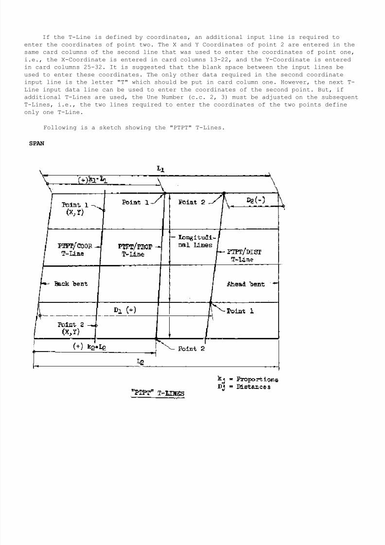
7/21/2019 Georgia Skew
http://slidepdf.com/reader/full/georgia-skew 111/182
If the T-Line is defined by coordinates, an additional input line is required to
enter the coordinates of point two. The X and Y Coordinates of point 2 are entered in the
same card columns of the second line that was used to enter the coordinates of point one,
i.e., the X-Coordinate is entered in card columns 13-22, and the Y-Coordinate is entered
in card columns 25-32. It is suggested that the blank space between the input lines be
used to enter these coordinates. The only other data required in the second coordinate
input line is the letter "T" which should be put in card column one. However, the next T-
Line input data line can be used to enter the coordinates of the second point. But, if
additional T-Lines are used, the Une Number (c.c. 2, 3) must be adjusted on the subsequent
T-Lines, i.e., the two lines required to enter the coordinates of the two points define
only one T-Line.
Following is a sketch showing the "PTPT" T-Lines.
SPAN
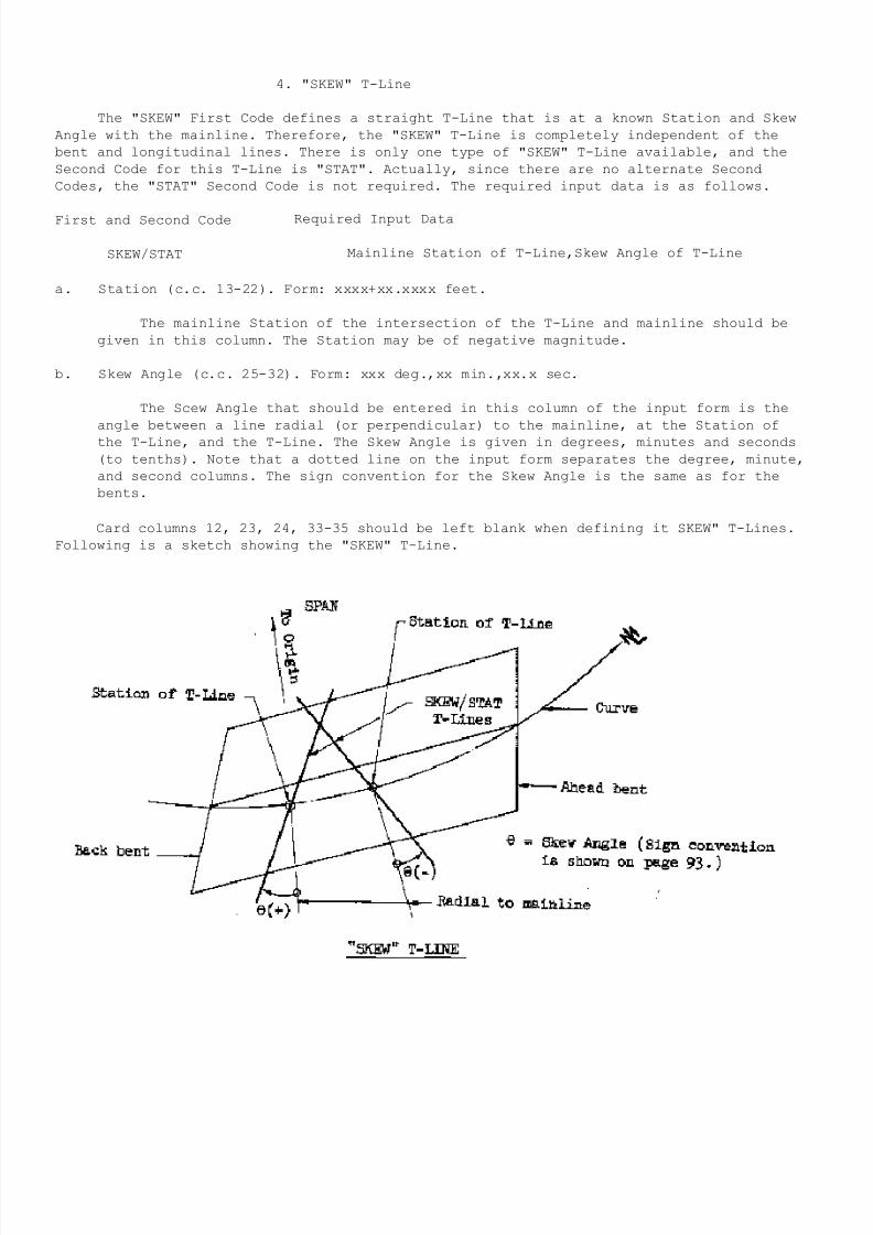
7/21/2019 Georgia Skew
http://slidepdf.com/reader/full/georgia-skew 112/182
4. "SKEW" T-Line
The "SKEW" First Code defines a straight T-Line that is at a known Station and Skew
Angle with the mainline. Therefore, the "SKEW" T-Line is completely independent of the
bent and longitudinal lines. There is only one type of "SKEW" T-Line available, and the
Second Code for this T-Line is "STAT". Actually, since there are no alternate Second
Codes, the "STAT" Second Code is not required. The required input data is as follows.
First and Second Code Required Input Data
SKEW/STAT Mainline Station of T-Line,Skew Angle of T-Line
a. Station (c.c. 13-22). Form: xxxx+xx.xxxx feet.
The mainline Station of the intersection of the T-Line and mainline should be
given in this column. The Station may be of negative magnitude.
b. Skew Angle (c.c. 25-32). Form: xxx deg.,xx min.,xx.x sec.
The Scew Angle that should be entered in this column of the input form is the
angle between a line radial (or perpendicular) to the mainline, at the Station of
the T-Line, and the T-Line. The Skew Angle is given in degrees, minutes and seconds
(to tenths). Note that a dotted line on the input form separates the degree, minute,
and second columns. The sign convention for the Skew Angle is the same as for the
bents.
Card columns 12, 23, 24, 33-35 should be left blank when defining it SKEW" T-Lines.
Following is a sketch showing the "SKEW" T-Line.
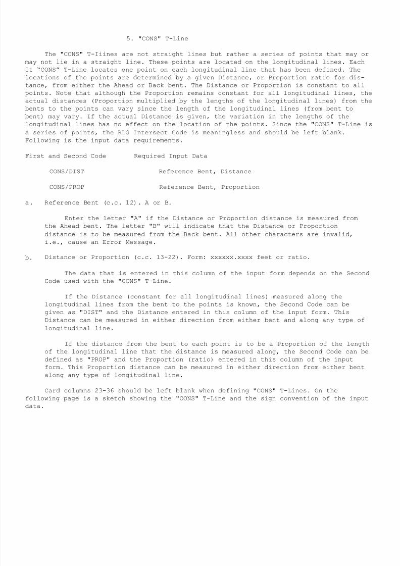
7/21/2019 Georgia Skew
http://slidepdf.com/reader/full/georgia-skew 113/182
5. "CONS" T-Line
The "CONS" T-Iiines are not straight lines but rather a series of points that may or
may not lie in a straight line. These points are located on the longitudinal lines. Each
It “CONS” T-Line locates one point on each longitudinal line that has been defined. The
locations of the points are determined by a given Distance, or Proportion ratio for dis-
tance, from either the Ahead or Back bent. The Distance or Proportion is constant to all
points. Note that although the Proportion remains constant for all longitudinal lines, the
actual distances (Proportion multiplied by the lengths of the longitudinal lines) from the
bents to the points can vary since the length of the longitudinal lines (from bent to
bent) may vary. If the actual Distance is given, the variation in the lengths of the
longitudinal lines has no effect on the location of the points. Since the "CONS" T-Line is
a series of points, the RLG Intersect Code is meaningless and should be left blank.
Following is the input data requirements.
First and Second Code Required Input Data
CONS/DIST Reference Bent, Distance
CONS/PROP Reference Bent, Proportion
a. Reference Bent (c.c. 12). A or B.
Enter the letter "A" if the Distance or Proportion distance is measured from
the Ahead bent. The letter "B" will indicate that the Distance or Proportion
distance is to be measured from the Back bent. All other characters are invalid,
i.e., cause an Error Message.
b. Distance or Proportion (c.c. 13-22). Form: xxxxxx.xxxx feet or ratio.
The data that is entered in this column of the input form depends on the Second
Code used with the "CONS" T-Line.
If the Distance (constant for all longitudinal lines) measured along thelongitudinal lines from the bent to the points is known, the Second Code can be
given as "DIST" and the Distance entered in this column of the input form. This
Distance can be measured in either direction from either bent and along any type of
longitudinal line.
If the distance from the bent to each point is to be a Proportion of the length
of the longitudinal line that the distance is measured along, the Second Code can be
defined as "PROP" and the Proportion (ratio) entered in this column of the input
form. This Proportion distance can be measured in either direction from either bent
along any type of longitudinal line.
Card columns 23-36 should be left blank when defining "CONS" T-Lines. On the
following page is a sketch showing the "CONS" T-Line and the sign convention of the inputdata.
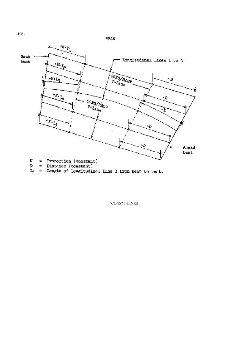
7/21/2019 Georgia Skew
http://slidepdf.com/reader/full/georgia-skew 114/182
- 106 -
"CONS" T-LINES
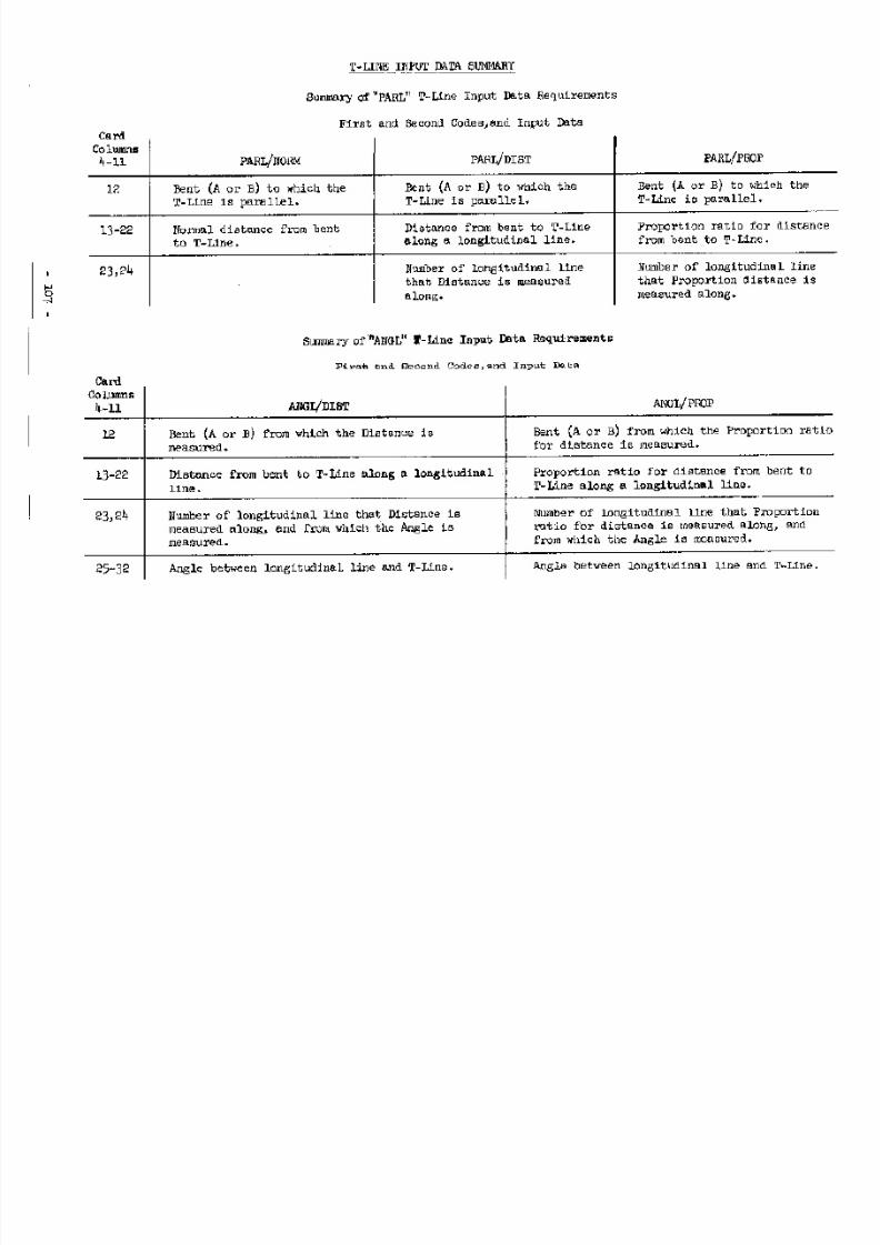
7/21/2019 Georgia Skew
http://slidepdf.com/reader/full/georgia-skew 115/182
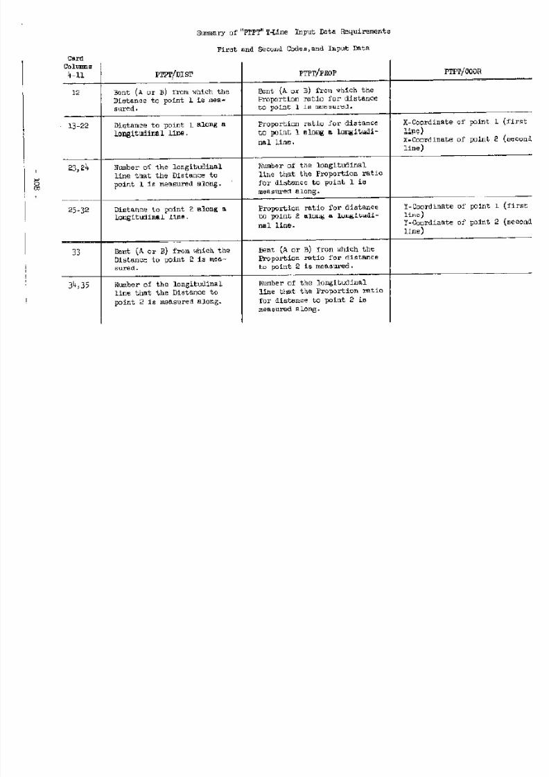
7/21/2019 Georgia Skew
http://slidepdf.com/reader/full/georgia-skew 116/182
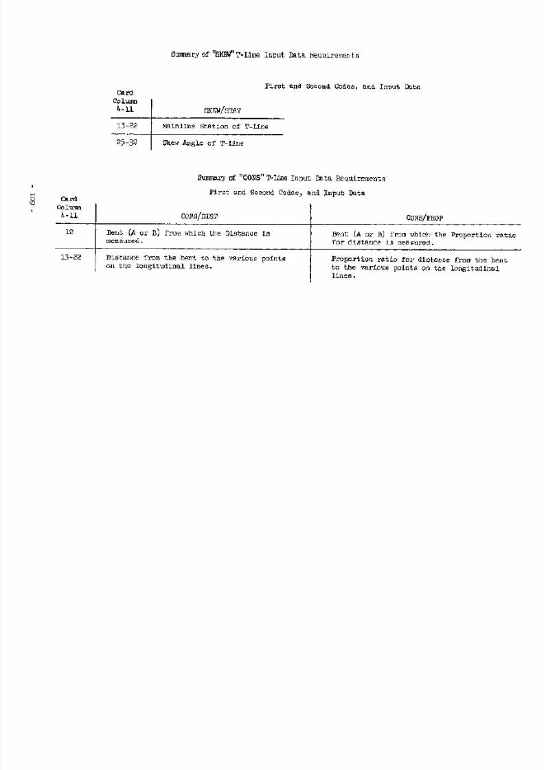
7/21/2019 Georgia Skew
http://slidepdf.com/reader/full/georgia-skew 117/182
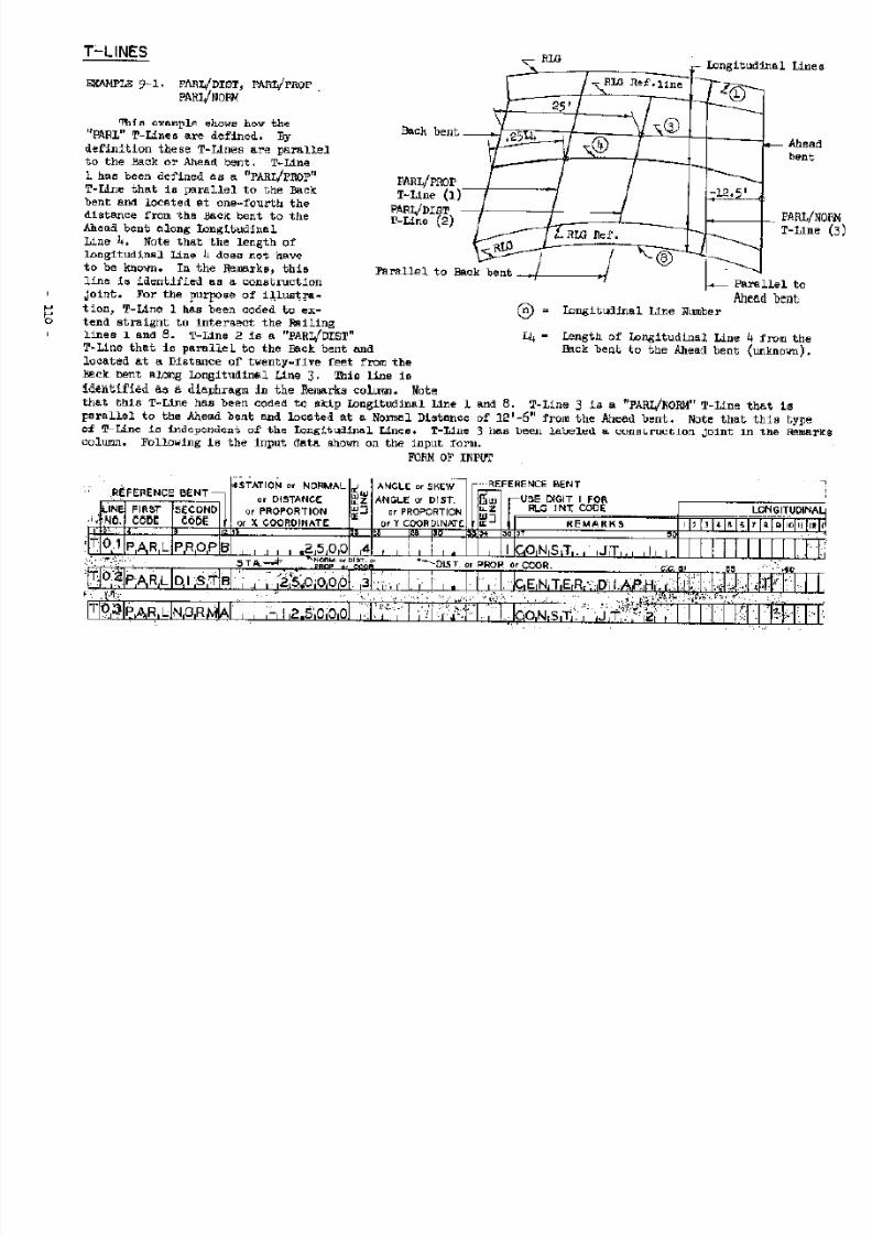
7/21/2019 Georgia Skew
http://slidepdf.com/reader/full/georgia-skew 118/182
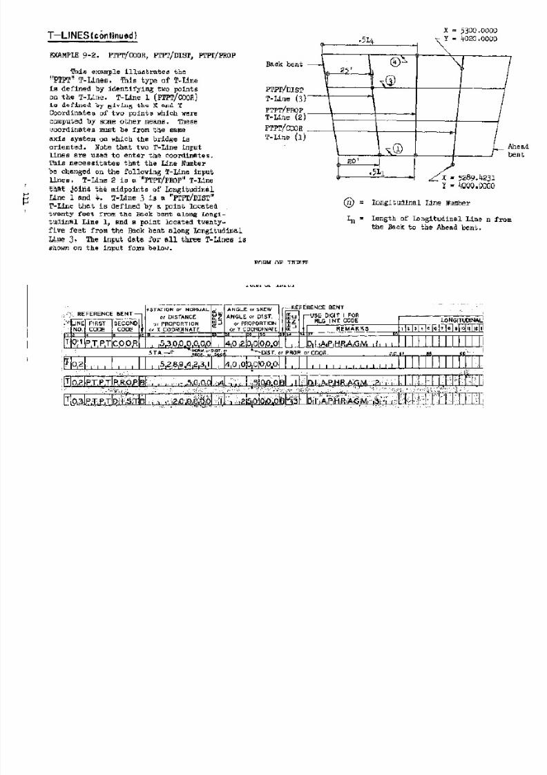
7/21/2019 Georgia Skew
http://slidepdf.com/reader/full/georgia-skew 119/182
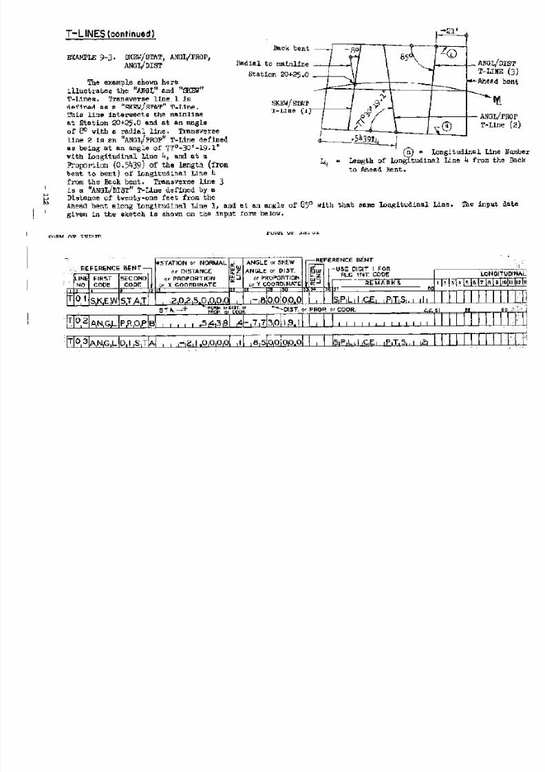
7/21/2019 Georgia Skew
http://slidepdf.com/reader/full/georgia-skew 120/182
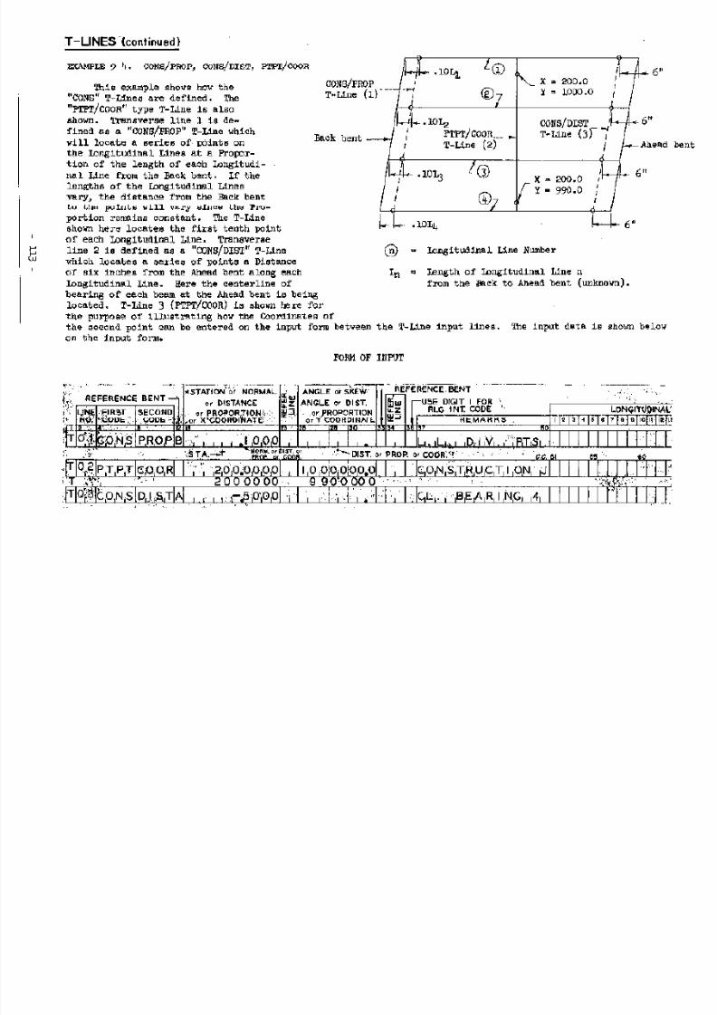
7/21/2019 Georgia Skew
http://slidepdf.com/reader/full/georgia-skew 121/182
7/21/2019 Georgia Skew
http://slidepdf.com/reader/full/georgia-skew 122/182
COORDINATE TYPE INPUT
Tile COORDINATE input form is used to enter the coordinates of known points on the
bridge. Therefore, the coordinate input must be computed by hand or by some other program.
The program requires that the bridge and the coordinate input data be oriented on the same
X and Y coordinate axis system. The Coordinate input data can be used in lieu of, or in
conjunction with, the Span input data. That is, the program can compute the intersections
of T-Lines and longitudinal lines of a span and then compute the various output data from
Coordinate input data, or vice versa, all in the same problem. If the point defining input
data consists solely of coordinates (no Span Data), the first Coordinate input sheet
should follow the Longitudinal Line input data sheet. Although the longitudinal lines are
not used when computing the output data for the coordinate input data, at least one
longitudinal line must always be defined when using point defining input data that
consists entirely of coordinates. When Coordinate and Span input data are used in the same
problem, the sequence of the Coordinate and Span input data is immaterial.
The program has the capacity for related coordinate points to be grouped into units,
analogous to the Span input data, by using two or more sheets of Coordinate input data.
The program will skip to the beginning of a new page when a new unit (another input sheet)
is given.
The COORDINATE input data form consists of two types of input data lines. They are:
Coordinate Identification and Coordinate Point.
A. Coordinate Identification (8COOR in c.c. 1-5).
The Coordinate Identification is used to identify each unit of related points.
This input line should always be filled in except in the following case. If more than
thirty points are in a unit, a second Coordinate input sheet can be used to enter the
remaining points after thirty points have been entered on the first Coordinate sheet.
The Coordinate Identification of the second sheet of Coordinate input would be left
blank.
The total Number of Points in the unit should be entered in card columns 10, 11.This number should not be zero nor greater than ninety-nine. Whenever the last unit
of coordinates are entered, and no Span Data is to follow, the code "LAST" should be
entered in card columns 13-16. This signifies that after processing the unit of
coordinate points the problem is to be terminated. Any pertinent Remarks that
describe the unit of coordinate points are entered in card columns 18-48. These
Remarks will head the output listing of each unit.
B. Coordinate Point (CP in c.c. 1,2).
Each COORDINATE input form contains thirty (30) Coordinate Point input lines.
The X and Y coordinates of each point are entered on one Coordinate Point input line.
There is no limitation on the number of points that can be entered except that only
ninety-nine are allowed per unit. However, any number of units may be used. A
Sequence Number is given it card columns 3, 4. However, the sequence of the points is
not checked by the program. This number will appear in the output data of each point.
7/21/2019 Georgia Skew
http://slidepdf.com/reader/full/georgia-skew 123/182
1. Point Identification (c.c. 5-8).
This space is provided so that each point can be labeled with a short alphabetic
or numeric code. This information will be given in the output data of each point. If
the Sequence Number is sufficient to identify the point, this space can be left
blank.
2. X-Coordinate (c.c. 9-18). Form: xxxxxx.xxxx feet.
Enter in this column the X-Coordinate of the point. This coordinate can be zero
only when the Y-Coordinate is not zero.
3. Y-Coordinate (c.c. 19-28). Form: xxxxxx.xxxx feet.
Enter in this column the Y-Coordinate of the point. This coordinate can be zero
only when the X-Coordinate is not zero.
4. Remarks (c.c. 29-48).
Enter in these card columns any pertinent Remarks that describe the point. These
Remarks will be given in the output data of each point.
The output data of each point consists of the following information.
1. Sequence Number of point.
2. Station of point.
3. Finished grade elevation of point.
4. Distance (radial or perpendicular to mainline) from point to mainline.
5. X-Coordinate of point.
6. Y-Coordinate of point.
7- Point Identification.
8. Remarks.
7/21/2019 Georgia Skew
http://slidepdf.com/reader/full/georgia-skew 124/182
IV. THE OUTPUT DATA
In the following discussion of The Output Data,, refer to the output data of one of
the example problems. All dimensions (Distances), Stations, Elevations)and Coordinates are
given in feet. Angles are given in degrees, minutes, and seconds (to tenths).
The output data will contain in addition to the data computed by the program, the
input data given on the input data forms. This input data listing can be used to check
against the data entered on the input forms and, in addition, used as a permanent part of
the record of the problem. The first page of the output data is a listing of the layout
Data which is given on the first page of the input data forms. Suitable headings are given
so that this output is easily recognized. All blank numeric input data fields are listed
as zero.
The second page of the output data is a listing of the Longitudinal Lines, also with
headings. The heading "DR / Xl" indicates that the data in that column is a "∆ R"
dimension or X-Coordinate. The heading "STA./ Yl" identifies the data in that column as a
Station or Y-Coordinate. The heading "TR / R / X2" indicates a Taper Rate, Radius, or X-
Coordinate is listed in that column. The data listed in the columns of the headings
mentioned above depends on the type of longitudinal line. Whenever more than one set of
Longitudinal lines is used, the additional Longitudinal Lines are listed in the outputdata when they appear in the input data, i.e., immediately following the output data of
the preceding span.
The input data of each span with headings is listed in the output data immediately
preceding the computed output data for that span. The heading "STA./NORM." given in the
Bent Data identifies the data in that column as a Station or Normal distance. The heading
"S/N/D/P/X" given in the listing of the T-Line input data indicates that the data in that
column is a Station, Normal distance, Distance, Proportion or X-Coordinate, depending on
the type of T-Line being listed. The heading "A/S/D/P/Y" identifies the data in that
column as an Angle, Skew angle, Distance, Proportion, or Y-Coordinate, again depending on
the type of T-Line being listed.
THE SPAN OUTPUT DATA
The Span Output Data will contain the various computed data for each point of
intersection of the longitudinal lines with the T-Lines. The first line of the Span Output
will contain the Span Number and Problem Number for identification.
Bent Data
The Bent Data of the Span Output Data contains the Bent designation (A or B), Bent
Number, Station, Skew Angle, Remarks, and Type for each of the two bents that defines the
span. The Station of the bent is the station of the point of intersection of the bent with
the mainline. The Skew Angle is the angle between a line radial to the mainline at the
Bent Station and the bent line. The same sign convention applies to the output Skew Angle
that applies to the input Skew Angles. If the Station and Skew Angle of the bent are not
given in the input data, the program will compute this data. Therefore, the program can be
used to compute bent Skew Angles and Stations when they are not otherwise known. The Bent
Number, Remarks and Type are a repeat of the input data. The Bent designation "A"
identifies the Ahead bent, and "B" identifies the Back bent. The Bent Data of the Back
bent is listed first, and the data for the Ahead bent is listed immediately following.
7/21/2019 Georgia Skew
http://slidepdf.com/reader/full/georgia-skew 125/182
Longitudinal Line Output
The data computed for the points of intersection of the bents and T-Lines with a
longitudinal line is given in the output of that longitudinal line. The heading for the
output of each longitudinal line will contain the Sequence Number, Type and Remarks that
were given in the input data when defining the longitudinal line. Following is an example.
"LONG. LINE 4 CRD BEAM C"
The next line of the output data contains the headings for the data computed at the points
of intersection of the bent and T-Lines with the longitudinal line.
All intersections with longitudinal line one (1) are listed first. The data for one
intersection point is given on each line, and this data is listed immediately below the
longitudinal line and data headings. The number of intersection points (lines) given in
each longitudinal line output will depend on the number of T-Lines, and the number of T-
Lines coded to skip that longitudinal line. For example, if T-Line two (2) has been coded
to skip longitudinal line one (1), this T-Line will not appear in the output of
longitudinal line one. The data for the Back bent intersection with the longitudinal lineis listed first. Next, the data for the intersections of the T-Lines with the longitudinal
line is given, and in the same order that the T-Lines were defined in the Span Data input.
After the T-Line intersection data is listed, the data for the Ahead bent intersection
with the longitudinal line is given. This process of listing the intersection point data
for the Back bent, T-Lines, and Ahead bent with a longitudinal line is repeated for each
longitudinal line beginning with longitudinal line one (1). Note that when a longitudinal
line has been coded to be skipped (used as reference line only), the longitudinal line
will not appear in the output data and, therefore, the intersection point data of the
bents and T-Lines with that longitudinal line will be omitted in the output data. In
contrast, when a T-Line is coded to skip a longitudinal line, only one intersection point
is skipped in the output for each code used. For example, if T-Line two (2) is coded to
skip only longitudinal line four (4), the intersection data of this T-Line with the other
longitudinal lines will be given in the output data of those longitudinal lines.
The Distances, Stations, Elevations, and Coordinates listed in the output data are
given to four decimal positions and have been rounded off to the nearest ten-thousandth.
If the fractional part is exactly equal to zero, only one decimal position (a zero) is
given. Beginning on the next page is a discussion of the data given in the output of each
point of intersection of a T-Line or bent with a longitudinal line. The output data
headings are shown in parentheses.
7/21/2019 Georgia Skew
http://slidepdf.com/reader/full/georgia-skew 126/182
1. Transverse Line Notation (T-LINE).
The data for the intersection point of a T-Line or bent with the longitudinal
line is given on one output data line. The T-Line Notation is used to identify the
transverse line for which the data is given. The longitudinal line will have been
noted in the longitudinal line heading. The letter "B" indicates the transverse line
is a bent, and the letter "T" identifies a T-Line. In addition to the letter Code (B
or T), the T-Line Notation will include the Bent Number or Line Number of the T-Line,
whichever the case may be. Following is an example of the T-Line Notations. Assumethat the intersection data being given is for longitudinal line two (2). Explanations
are given in parentheses.
T-LINE (Output data headings listed on this line.)
B 1 (Bent 1 (Back) intersection with longitudinal line 2 data.)
T 1 (T-Line 1 intersection with longitudinal line 2 data.)
T 2 (T-Line 2 intersection with longitudinal line 2 data.)
T 4 (T-Line 4 intersection with longitudinal line 2 data.)
B 2L (Bent 2L (Ahead) intersection with longitudinal line 2 data.)
Note that T-Line 3 is not shown in the above example. This indicates that T-Line 3
was coded to skip the intersection with longitudinal line 2.
In order to locate the output data for the intersection of T-Line I with
longitudinal line J, first locate the output data of longitudinal line J. Then find
the Transverse Line Notation for T-Line I in the column headed by "T-LINE". The line
on which the Transverse Line Notation (T I) is found contains the desired data.
2. Station of Intersection Point (STATION).
The output data in this column is the station (measured along the mainline) of
the point of intersection of the T-Line (or bent) with the longitudinal line. Since
the point usually will not be located on the mainline, the mainline station is found
by projecting the point radially (or perpendicular) to the mainline. Note that a plus
sign (+) has been included in the station for clarity and consistence with normal
practice.
3. Elevation of Intersection Point (ELEVATION).
The elevation listed in this column of output data is the finished grade (bridge
surface) elevation of the point of intersection of the T-Line (or bent) with the
longitudinal line. This elevation is computed by first determining the profile grade
elevation of the station of the intersection point. Then the elevation is correctedfor the bridge crown whether the crown is a parabola or superelevated (constant or
transition).
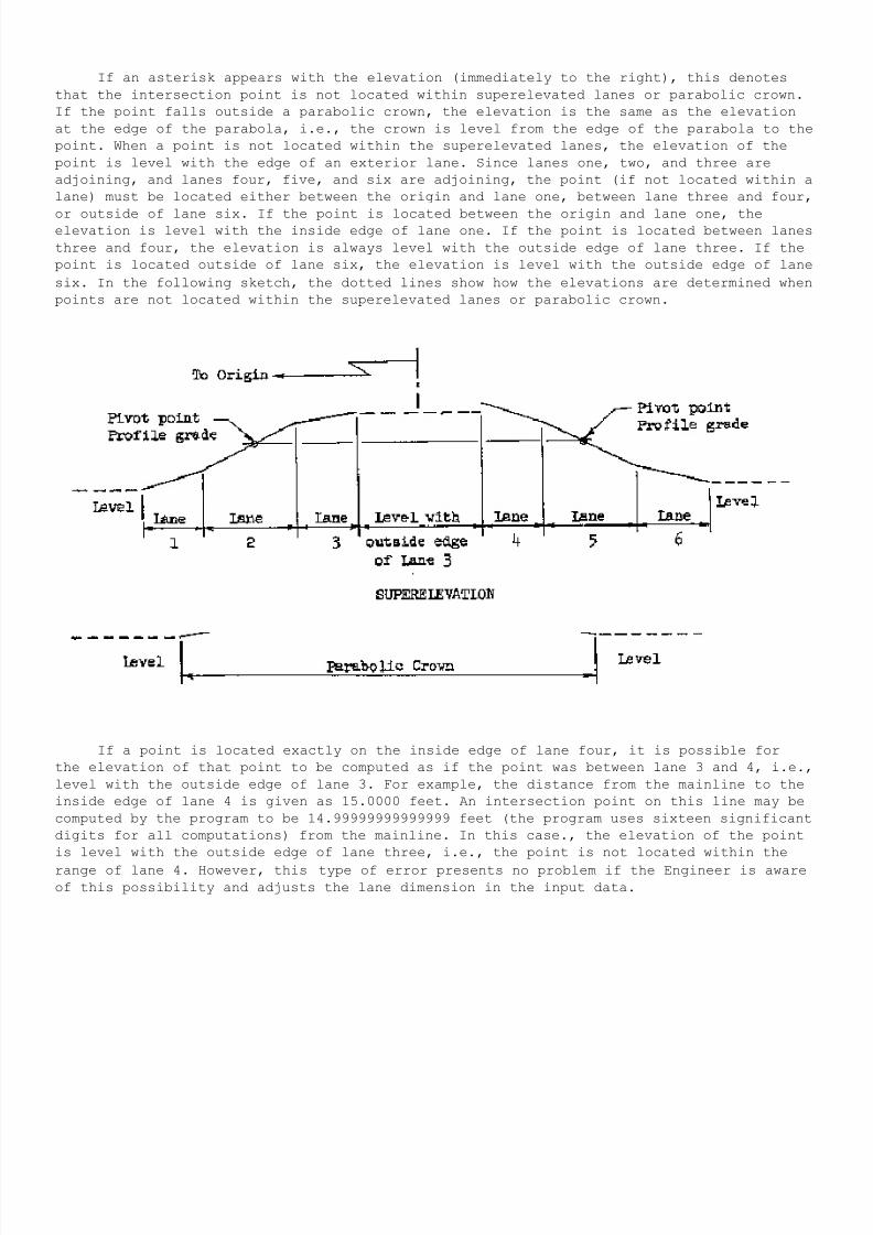
7/21/2019 Georgia Skew
http://slidepdf.com/reader/full/georgia-skew 127/182
If an asterisk appears with the elevation (immediately to the right), this denotes
that the intersection point is not located within superelevated lanes or parabolic crown.
If the point falls outside a parabolic crown, the elevation is the same as the elevation
at the edge of the parabola, i.e., the crown is level from the edge of the parabola to the
point. When a point is not located within the superelevated lanes, the elevation of the
point is level with the edge of an exterior lane. Since lanes one, two, and three are
adjoining, and lanes four, five, and six are adjoining, the point (if not located within a
lane) must be located either between the origin and lane one, between lane three and four,
or outside of lane six. If the point is located between the origin and lane one, theelevation is level with the inside edge of lane one. If the point is located between lanes
three and four, the elevation is always level with the outside edge of lane three. If the
point is located outside of lane six, the elevation is level with the outside edge of lane
six. In the following sketch, the dotted lines show how the elevations are determined when
points are not located within the superelevated lanes or parabolic crown.
If a point is located exactly on the inside edge of lane four, it is possible for
the elevation of that point to be computed as if the point was between lane 3 and 4, i.e.,
level with the outside edge of lane 3. For example, the distance from the mainline to the
inside edge of lane 4 is given as 15.0000 feet. An intersection point on this line may be
computed by the program to be 14.99999999999999 feet (the program uses sixteen significant
digits for all computations) from the mainline. In this case., the elevation of the point
is level with the outside edge of lane three, i.e., the point is not located within the
range of lane 4. However, this type of error presents no problem if the Engineer is awareof this possibility and adjusts the lane dimension in the input data.
7/21/2019 Georgia Skew
http://slidepdf.com/reader/full/georgia-skew 128/182
The program assumes that the width of each lane of superelevation remains
constant throughout the range of the problem and that the rate of superelevation is
given radial (or perpendicular) to the lane. If the width of a lane actually varies,
or for some reason the superelevation rate is not radial (or perpendicular) to the
mainline, some elevations given in the output may have to be corrected. These
corrections would depend upon their location.
4. Distance from Point to Mainline (DT TO ML).
The distance listed in this column is from the point of intersection of the T-
Line (or bent) with the longitudinal line to the mainline. This distance is always
measured on a radial or perpendicular line to the mainline depending on the type
(curve or tangent) of mainline. If the distance is negative, the point is located on
the origin side of the mainline; otherwise (positive), the point is located on the
side of the mainline away from the origin. If the dimension is zero, the point is
located on the mainline.
5. Distance from Point to Back Bent (DT TO BT).
The output data listed in this column is the distance from the point of
intersection of the T-Line (or bent) with the longitudinal line to the Back bent.
This distance is measured along the longitudinal line, regardless whether the
longitudinal line is a curve or straight line, or a combination of both. If the
distance is negative, this indicates that the point is back of the Back bent and
located on the longitudinal line extended back from the Back bent (the point is not
necessarily located on the same longitudinal line of the previous span). If the point
is ahead of the Ahead bent, the point is located on the longitudinal line extended
forward from the Ahead bent. This distance will be zero if the transverse line is the
Back bent.
Note that the distance given for the Ahead bent intersection point will be the
length of the longitudinal line from the Back bent to the Ahead bent. If the Aheadbent is coded to skip the longitudinal line, the length of the longitudinal line will
not be listed in the output.
6. Distance from Point to Previous Point (DT TO PP).
This dimension is the distance from the point of intersection of the T-Line (or
bent) with the longitudinal line to the point of intersection of the same T-Line (or
bent) with the preceding longitudinal line. This distance, then, is measured along
the T-Line (or bent) from longitudinal line to longitudinal line. All distances given
for longitudinal line one are zero since in this case there is no preceding
longitudinal line in the span.
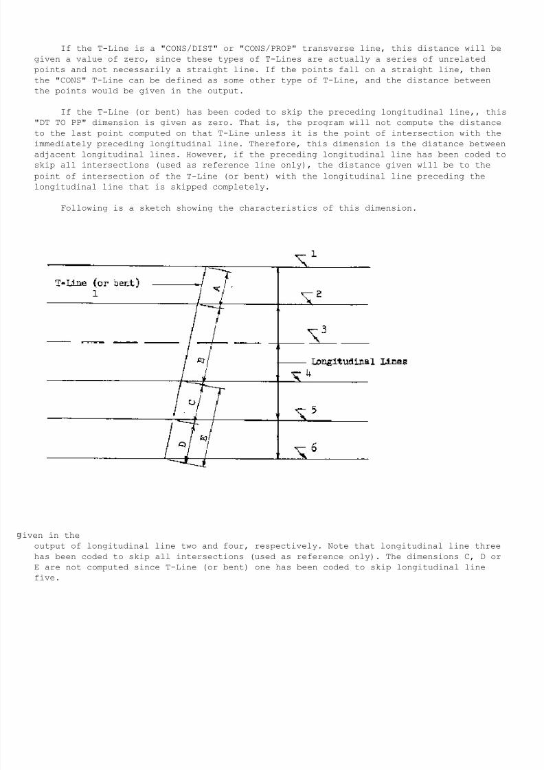
7/21/2019 Georgia Skew
http://slidepdf.com/reader/full/georgia-skew 129/182
If the T-Line is a "CONS/DIST" or "CONS/PROP" transverse line, this distance will be
given a value of zero, since these types of T-Lines are actually a series of unrelated
points and not necessarily a straight line. If the points fall on a straight line, then
the "CONS" T-Line can be defined as some other type of T-Line, and the distance between
the points would be given in the output.
If the T-Line (or bent) has been coded to skip the preceding longitudinal line,, this
"DT TO PP" dimension is given as zero. That is, the program will not compute the distance
to the last point computed on that T-Line unless it is the point of intersection with theimmediately preceding longitudinal line. Therefore, this dimension is the distance between
adjacent longitudinal lines. However, if the preceding longitudinal line has been coded to
skip all intersections (used as reference line only), the distance given will be to the
point of intersection of the T-Line (or bent) with the longitudinal line preceding the
longitudinal line that is skipped completely.
Following is a sketch showing the characteristics of this dimension.
iven in the
output of longitudinal line two and four, respectively. Note that longitudinal line three
has been coded to skip all intersections (used as reference only). The dimensions C, D or
E are not computed since T-Line (or bent) one has been coded to skip longitudinal line
five.
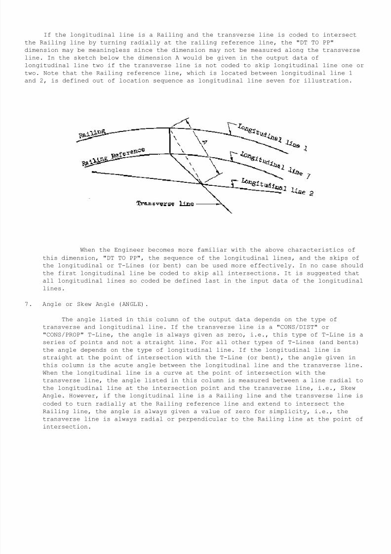
7/21/2019 Georgia Skew
http://slidepdf.com/reader/full/georgia-skew 130/182
If the longitudinal line is a Railing and the transverse line is coded to intersect
the Railing line by turning radially at the railing reference line, the "DT TO PP"
dimension may be meaningless since the dimension may not be measured along the transverse
line. In the sketch below the dimension A would be given in the output data of
longitudinal line two if the transverse line is not coded to skip longitudinal line one or
two. Note that the Railing reference line, which is located between longitudinal line 1
and 2, is defined out of location sequence as longitudinal line seven for illustration.
When the Engineer becomes more familiar with the above characteristics of
this dimension, "DT TO PP", the sequence of the longitudinal lines, and the skips of
the longitudinal or T-Lines (or bent) can be used more effectively. In no case should
the first longitudinal line be coded to skip all intersections. It is suggested that
all longitudinal lines so coded be defined last in the input data of the longitudinal
lines.
7. Angle or Skew Angle (ANGLE).
The angle listed in this column of the output data depends on the type of
transverse and longitudinal line. If the transverse line is a "CONS/DIST" or
"CONS/PROP" T-Line, the angle is always given as zero, i.e., this type of T-Line is a
series of points and not a straight line. For all other types of T-Lines (and bents)
the angle depends on the type of longitudinal line. If the longitudinal line is
straight at the point of intersection with the T-Line (or bent), the angle given in
this column is the acute angle between the longitudinal line and the transverse line.
When the longitudinal line is a curve at the point of intersection with the
transverse line, the angle listed in this column is measured between a line radial to
the longitudinal line at the intersection point and the transverse line, i.e., SkewAngle. However, if the longitudinal line is a Railing line and the transverse line is
coded to turn radially at the Railing reference line and extend to intersect the
Railing line, the angle is always given a value of zero for simplicity, i.e., the
transverse line is always radial or perpendicular to the Railing line at the point of
intersection.
7/21/2019 Georgia Skew
http://slidepdf.com/reader/full/georgia-skew 131/182
The sign convention for an output Skew Angle is the same as the sign convention
for a Skew Angle entered in the input data. An angle between the transverse and
longitudinal line has the same sign convention as the angle required in the input
data to define an "ANGL/DIST" or "ANGL/"PROP" T-Line.
8. X-Coordinate (X).
The X-Coordinate of the point of intersection of the transverse line with the
longitudinal line is listed in this column of the output data. This coordinate isdependent on the orientation of the bridge given in the Location Data of the input
data.
9. Y-Coordinate (Y).
The Y-Coordinate of the point of intersection of the transverse line with the
longitudinal line is listed in this column of the output data. This coordinate is
dependent on the orientation of the bridge given in the location Data of the input
data.
10. Transverse Line Remarks (REMARKS).
The identifying remarks given in the input data of the transverse lines arelisted in this column so that the intersection point can be easily recognized.
11. Transverse Line Type or Code (TYPE LINE).
This column contains the First and Second Code of a T-Line, or the Bent Type
when the bent intersection point data is given.
This procedure of listing the data for the points of intersections of the transverse
lines (Bents and T-Lines) with a longitudinal line is repeated for each longitudinal line
beginning with longitudinal line one. After the last longitudinal line data is given, the
processing of that span is complete, and the program proceeds to process any subsequent
span or unit of coordinate input.
THE COORDINATE OUTPUT DATA
The output data given for the coordinate type input data is similar to the Span
Output Data. The input data for each point is listed with the computed data for that
point. The computed data output (Station, Elevation, DT TO ML) is the same as for the
output data of the spans except that the point is defined by input data coordinates rather
than by intersecting two lines. Note that the "Distance to Bent" and "Distance to Previous
Point" dimensions and Angles are not given in this type of output since the coordinate
points are not associated with any transverse or longitudinal lines.
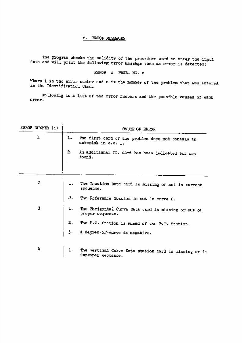
7/21/2019 Georgia Skew
http://slidepdf.com/reader/full/georgia-skew 132/182
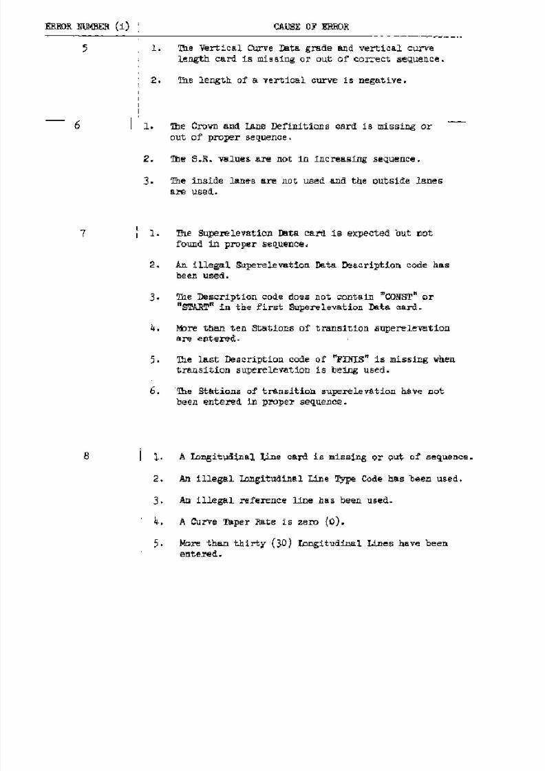
7/21/2019 Georgia Skew
http://slidepdf.com/reader/full/georgia-skew 133/182
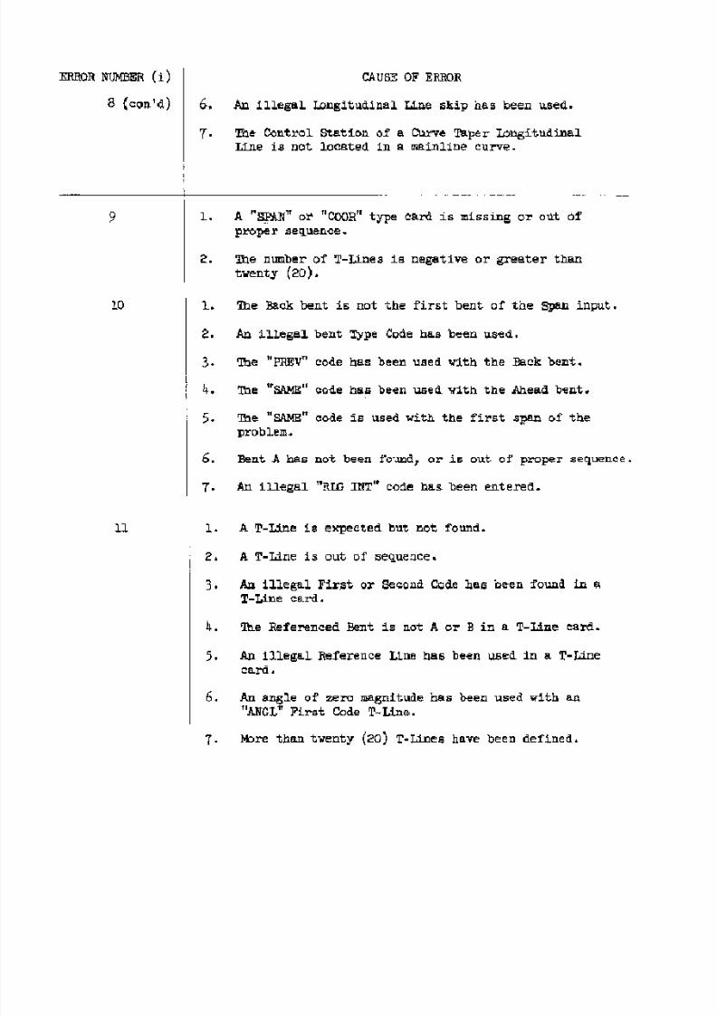
7/21/2019 Georgia Skew
http://slidepdf.com/reader/full/georgia-skew 134/182
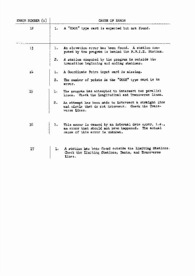
7/21/2019 Georgia Skew
http://slidepdf.com/reader/full/georgia-skew 135/182
7/21/2019 Georgia Skew
http://slidepdf.com/reader/full/georgia-skew 136/182
VI. EXAMPLE PROBLEM
Four Example Problems are given on the following pages for the purpose of
illustrating the procedure used to enter the input data on the input forms. In addition to
the input forms that contain the input data, a sketch of the bridge geometry and the
output data will be given with each example. These problems do not represent an actual
bridge structure. The examples are designed only to illustrate the numerous
characteristics of the program.
Example Number One
Example 1 shows a two-span bridge located in a 30 curve. The four beams of each span
are placed parallel to a centerline chord of that span, and the beams in the adjacent
spans meet at a common point (concentric arc intersection) at the centerline of Bent 2.
Bents 1 and 3 are parallel to Bent 2 and located by the known normal distances from Bent
2.
The Station of Bent 2 will be chosen as the Reference Point Station. Bents are
placed parallel to the Y-axis by using a Reference Angle of 720. The Limiting Stations are
arbitrarily chosen as 19+00 and 21+00. The roadway surface is at a constant rate of
superelevation. The curb faces and sidewalks are set up as lanes of superelevation. This
requires that six lanes of superelevation be defined. The Vertical Curve Data and
dimensions for defining the lanes of superelevation are given in the sketch along with the
superelevation rates.
Two sets of Longitudinal Lines are defined in the problem. The beams of Span 1 are
defined as PIA, and the beams of Span 2 are defined as PIB. Note that the centerline chord
and beam lines are from the centerline of Bent 2 to the B.F.P.R. (Back Face Paving Rest)
line of the end bents. The center lines of the railings are defined for the purpose of
computing lengths for rail spacings. In addition, the finished grade elevations at the
intersection of the railing lines with the bents will be given. Since the centerline chord
and gutter lines are used only as reference lines in this problem, these lines are coded
to be skipped in the output data.
The centerline-of-bearings and diaphragms are set up as T-Lines in each span. The
diaphragms of Span 1 are located at the one-third points of the centerline chord. The
positions of the diaphragms in Span 2 are detailed in the sketch. The centerline-of-
bearings in Span 1 are defined as "CONS/DIST" T-Lines. In Span 2 the centerline-of -
bearings are defined as "PARL/DIST” T-Lines. Note that in many instances a T-Line can be
defined by several combinations of T-Line Codes.
The purpose of this problem, in addition to the ones already stated, is to compute
the following data.
1. Finished grade elevations at centerline-of-bearings.
2. Lengths of beams and diaphragms.
3. Position of diaphragms along each beam.
4. Distance between beams along bent lines.
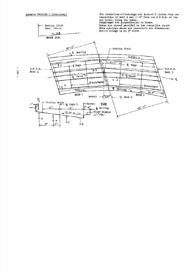
7/21/2019 Georgia Skew
http://slidepdf.com/reader/full/georgia-skew 137/182

7/21/2019 Georgia Skew
http://slidepdf.com/reader/full/georgia-skew 138/182
CROSS SECTION
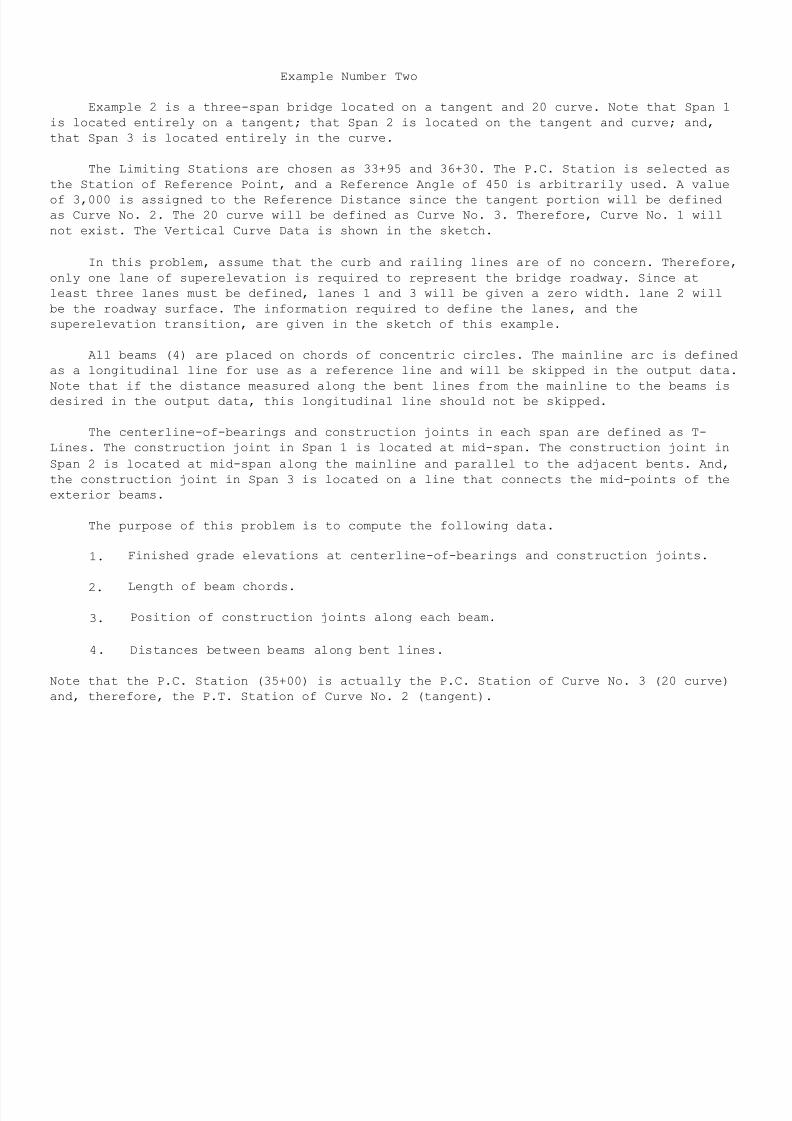
7/21/2019 Georgia Skew
http://slidepdf.com/reader/full/georgia-skew 139/182
Example Number Two
Example 2 is a three-span bridge located on a tangent and 20 curve. Note that Span 1
is located entirely on a tangent; that Span 2 is located on the tangent and curve; and,
that Span 3 is located entirely in the curve.
The Limiting Stations are chosen as 33+95 and 36+30. The P.C. Station is selected as
the Station of Reference Point, and a Reference Angle of 450 is arbitrarily used. A value
of 3,000 is assigned to the Reference Distance since the tangent portion will be defined
as Curve No. 2. The 20 curve will be defined as Curve No. 3. Therefore, Curve No. 1 will
not exist. The Vertical Curve Data is shown in the sketch.
In this problem, assume that the curb and railing lines are of no concern. Therefore,
only one lane of superelevation is required to represent the bridge roadway. Since at
least three lanes must be defined, lanes 1 and 3 will be given a zero width. lane 2 will
be the roadway surface. The information required to define the lanes, and the
superelevation transition, are given in the sketch of this example.
All beams (4) are placed on chords of concentric circles. The mainline arc is defined
as a longitudinal line for use as a reference line and will be skipped in the output data.
Note that if the distance measured along the bent lines from the mainline to the beams is
desired in the output data, this longitudinal line should not be skipped.
The centerline-of-bearings and construction joints in each span are defined as T-
Lines. The construction joint in Span 1 is located at mid-span. The construction joint in
Span 2 is located at mid-span along the mainline and parallel to the adjacent bents. And,
the construction joint in Span 3 is located on a line that connects the mid-points of the
exterior beams.
The purpose of this problem is to compute the following data.
1. Finished grade elevations at centerline-of-bearings and construction joints.
2. Length of beam chords.
3. Position of construction joints along each beam.
4. Distances between beams along bent lines.
Note that the P.C. Station (35+00) is actually the P.C. Station of Curve No. 3 (20 curve)
and, therefore, the P.T. Station of Curve No. 2 (tangent).
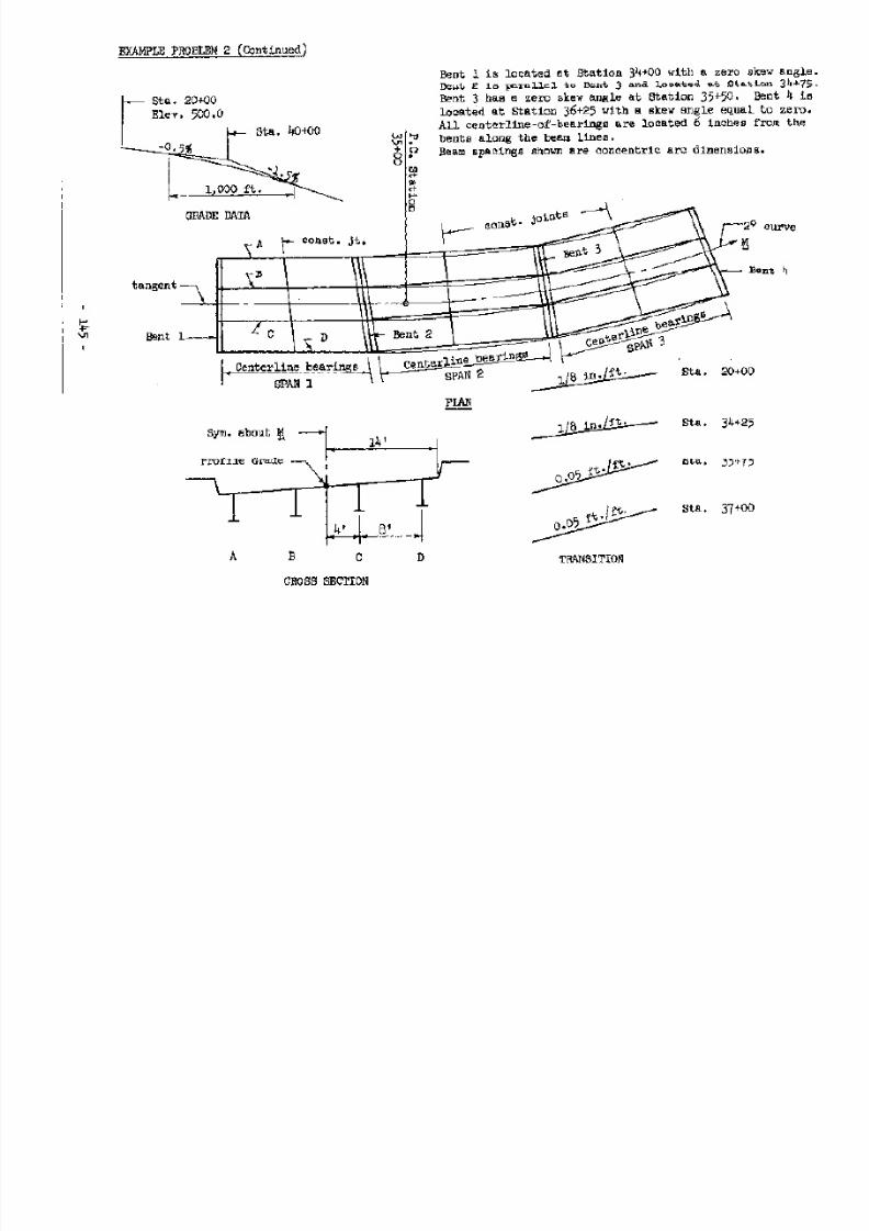
7/21/2019 Georgia Skew
http://slidepdf.com/reader/full/georgia-skew 140/182
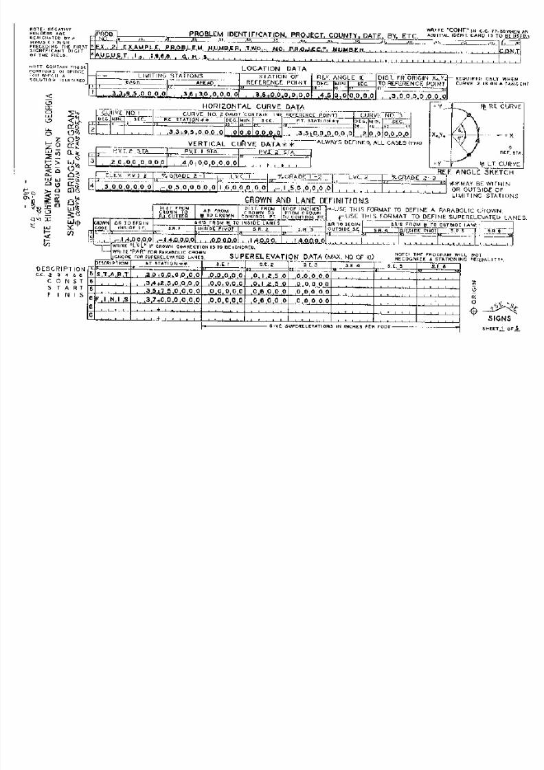
7/21/2019 Georgia Skew
http://slidepdf.com/reader/full/georgia-skew 141/182
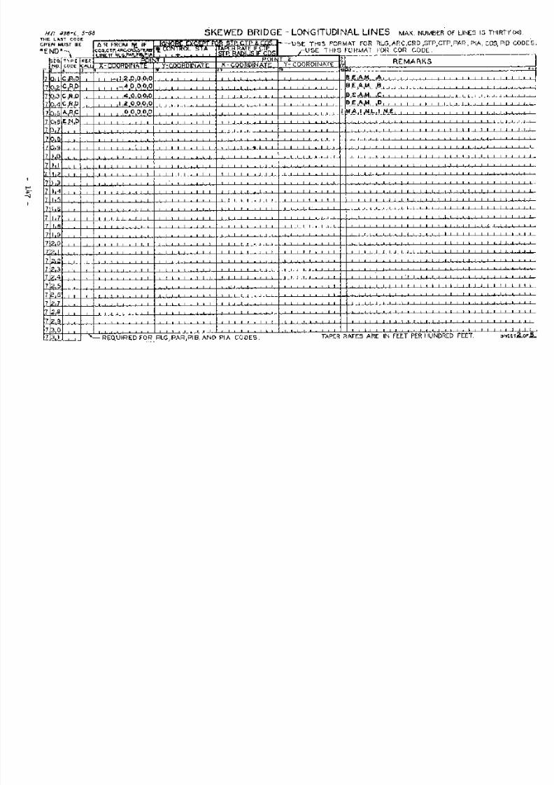
7/21/2019 Georgia Skew
http://slidepdf.com/reader/full/georgia-skew 142/182
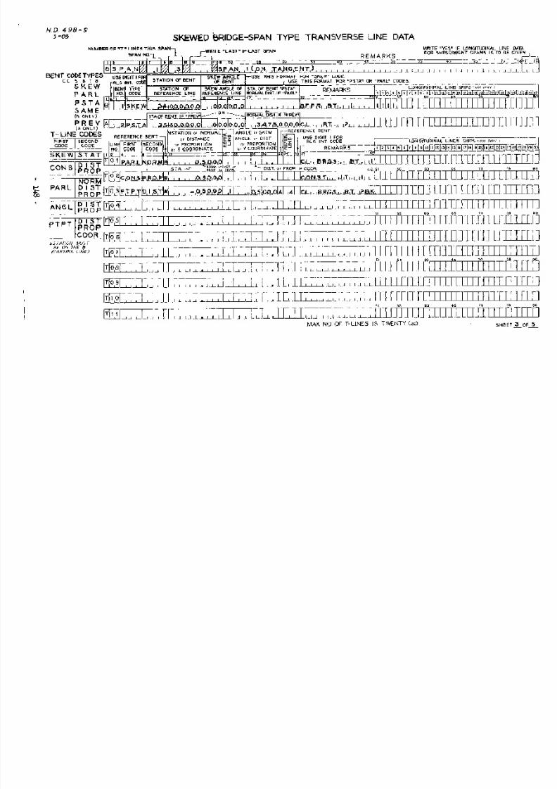
7/21/2019 Georgia Skew
http://slidepdf.com/reader/full/georgia-skew 143/182
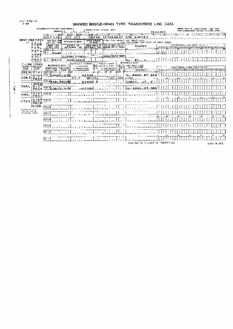
7/21/2019 Georgia Skew
http://slidepdf.com/reader/full/georgia-skew 144/182
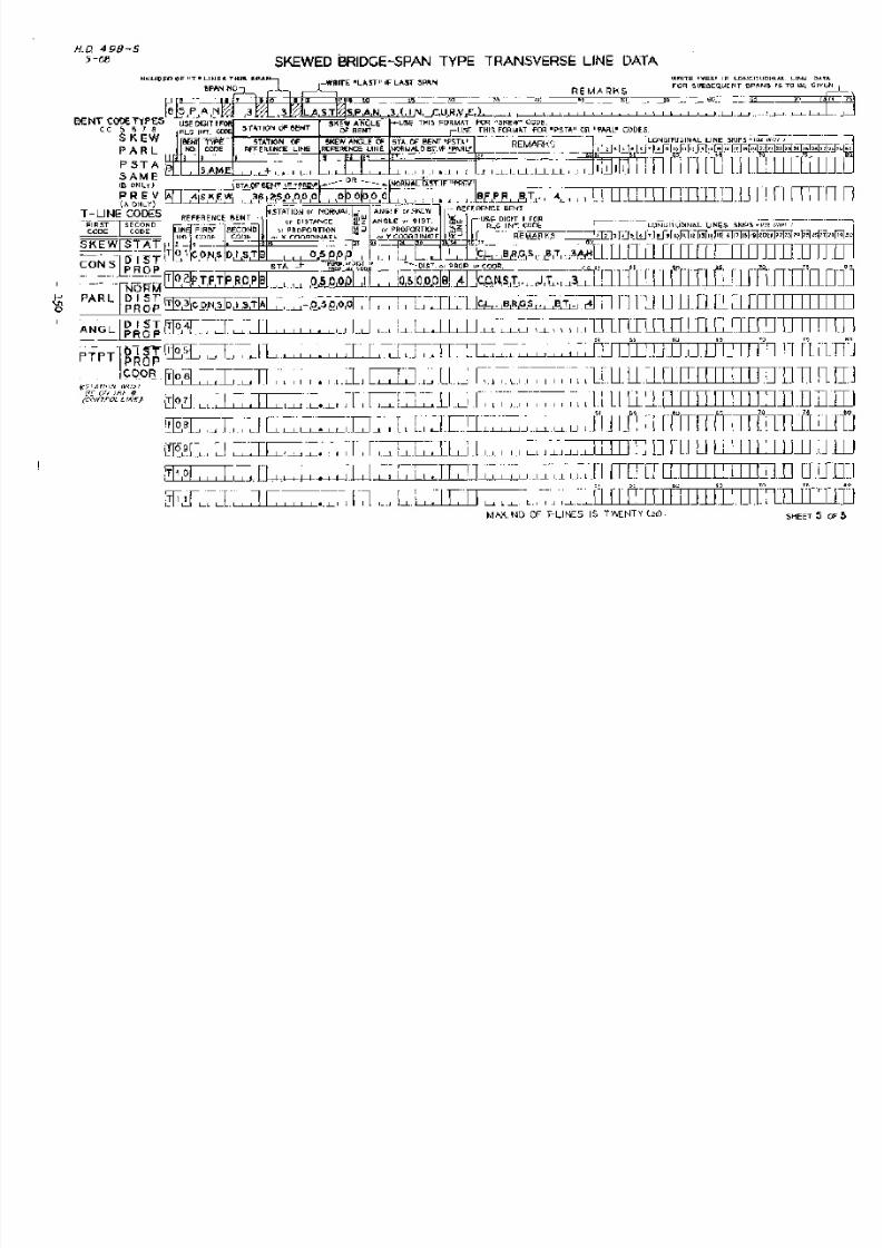
7/21/2019 Georgia Skew
http://slidepdf.com/reader/full/georgia-skew 145/182
7/21/2019 Georgia Skew
http://slidepdf.com/reader/full/georgia-skew 146/182
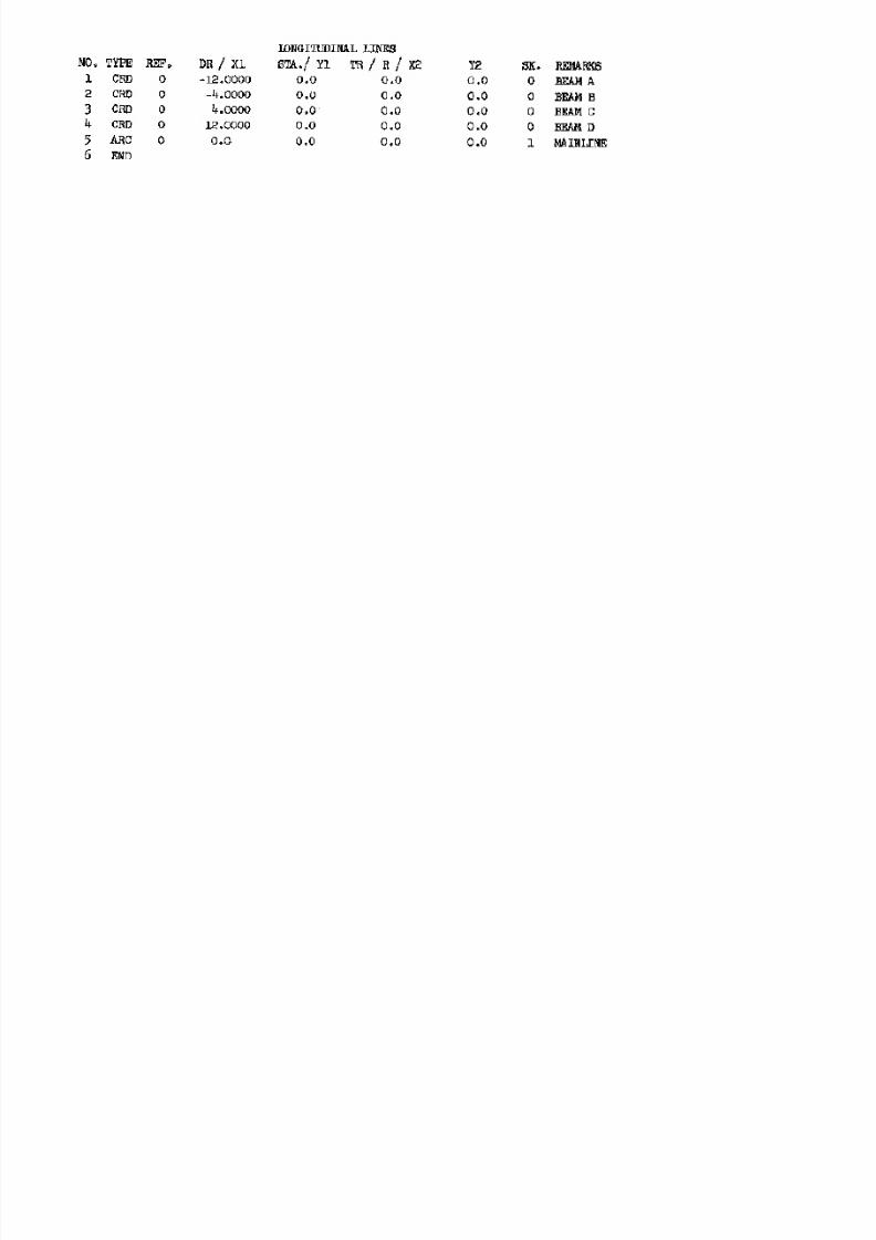
7/21/2019 Georgia Skew
http://slidepdf.com/reader/full/georgia-skew 147/182

7/21/2019 Georgia Skew
http://slidepdf.com/reader/full/georgia-skew 148/182
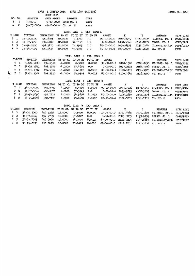
7/21/2019 Georgia Skew
http://slidepdf.com/reader/full/georgia-skew 149/182

7/21/2019 Georgia Skew
http://slidepdf.com/reader/full/georgia-skew 150/182
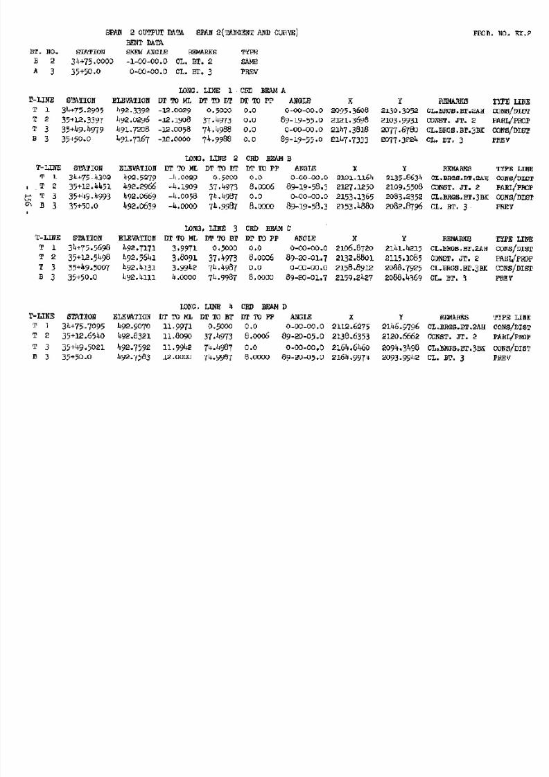
7/21/2019 Georgia Skew
http://slidepdf.com/reader/full/georgia-skew 151/182

7/21/2019 Georgia Skew
http://slidepdf.com/reader/full/georgia-skew 152/182
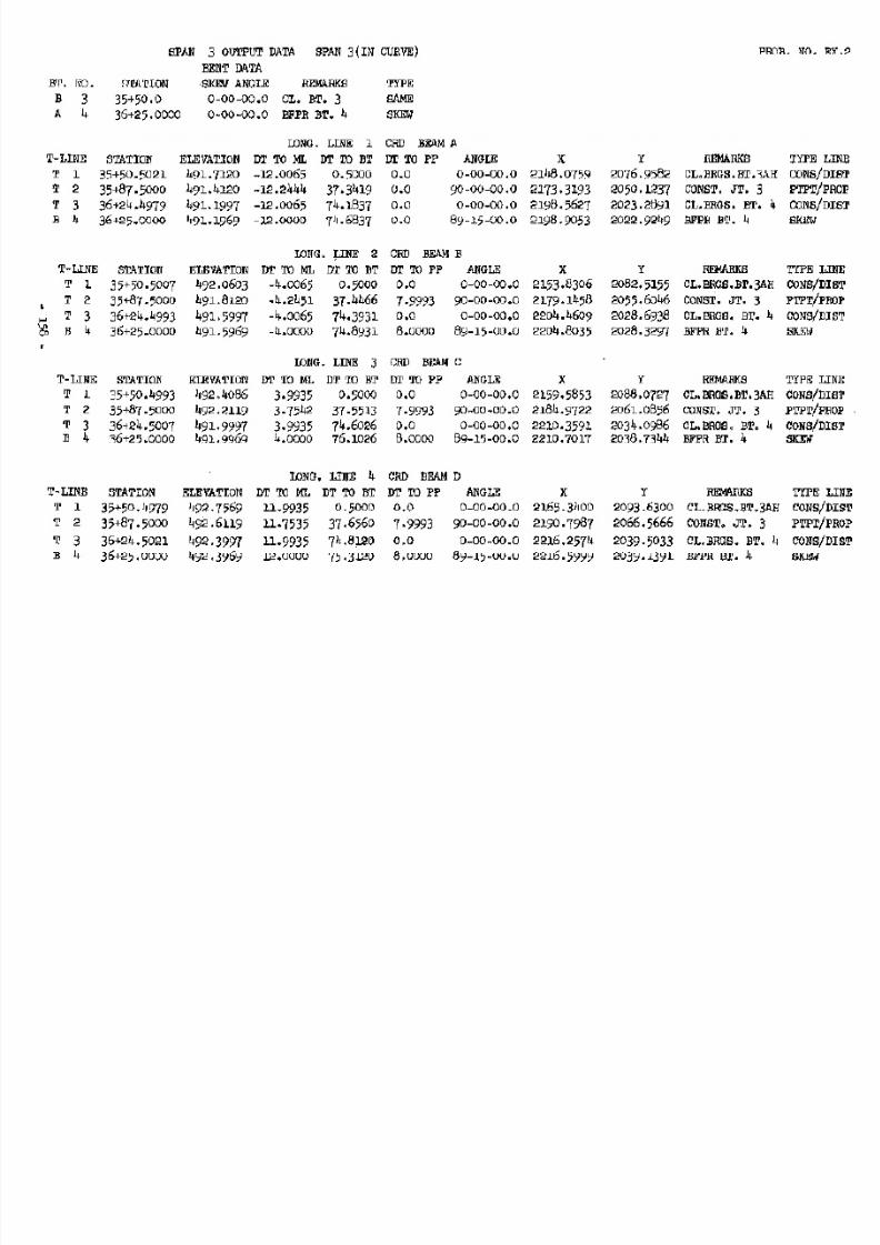
7/21/2019 Georgia Skew
http://slidepdf.com/reader/full/georgia-skew 153/182
7/21/2019 Georgia Skew
http://slidepdf.com/reader/full/georgia-skew 154/182
Example Number Three
Example 3 is a two-span bridge that is located on a tangent and 3 degree curve. Span
2 is located entirely within the curve, whereas Span 1 occupies a portion of the curve and
tangent. The Limiting Stations are chosen as 19+00 and 21+50. The Station of Reference
Point is selected as the P.C. Station, and a Reference Angle of 90 degrees is used in
order to place the tangent parallel to the X-axis. Therefore, a portion of Span 1 will be
placed in the second quadrant. Placing a bridge or portion of a bridge outside the first
quadrant is not recommended; however, this program solution will be valid. In this example
a working line is set up parallel to the tangent. The offset distance from the working
line to any intersection point given in the output can be computed conveniently by
subtracting a constant (Radius of 3 degrees curve plus four) from the Y-Coordinate of the
intersection point. And the distance along the working line from the P.C. Station to the
intersection point will be equal to the X-Coordinate of the point of intersection. The 3
degree curve will be defined as Curve No. 2, and the tangent will be defined as Curve No.
1. Curve No. 3 will not exist. Note that the Distance to Reference Point is not required
since Curve No. 2 is actually a circular curve.
In this example, it is assumed that the elevations are of no concern. Therefore, all
Grade Data is assigned a value of zero, and the roadway crown is defined as level.
The left side of the bridge (looking ahead) is in a taper throughout the entire
length of the bridge. In the tangent portion the gutter will be a Straight Taper, and in
the curve the gutter will conform to a Curve Taper (Spiral). The railing line is always at
a constant distance from the gutter line. The right gutter line in the tangent portion is
parallel to the mainline. However, in the curve portion the right gutter is a curve with a
radius of 1,500 feet and will be defined as a curve offset.
In this example, the gutter and railing lines must be defined twice, i.e., defined
for the tangent portion and again for the curve portion. The longitudinal lines defined
for the curve portion of the bridge will be skipped in the tangent portion of the bridge,
and vice versa. Note that if finished grade elevations were being computed, the elevations
in the shaded portion (varying width) and/or on the curbs would have to be adjusted
depending on the width assigned to the lane of superelevation that represents the roadway.
The line separating the tangent and curve (P.C. Station) will be defined as a T-Line
in Span 1. (An alternate way to set this problem up is to divide Span 1 into two spans
with the radial line at the P.C. Station as a bent line. Then define two sets of
longitudinal lines.) No beams or additional T-Lines are given in this example. The purpose
of the example is to compute the data necessary to define the curbs and railing in
relation to a working line, and the lengths along the railing lines.
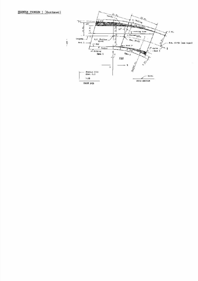
7/21/2019 Georgia Skew
http://slidepdf.com/reader/full/georgia-skew 155/182
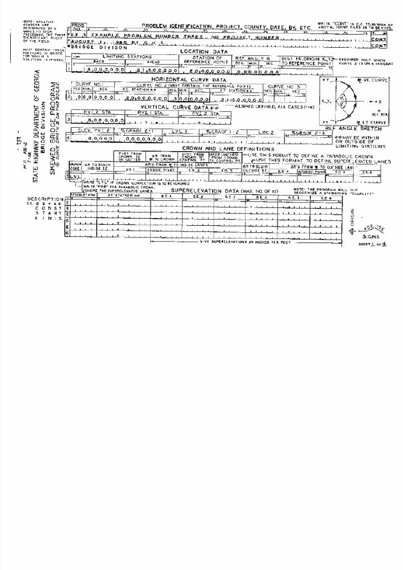
7/21/2019 Georgia Skew
http://slidepdf.com/reader/full/georgia-skew 156/182
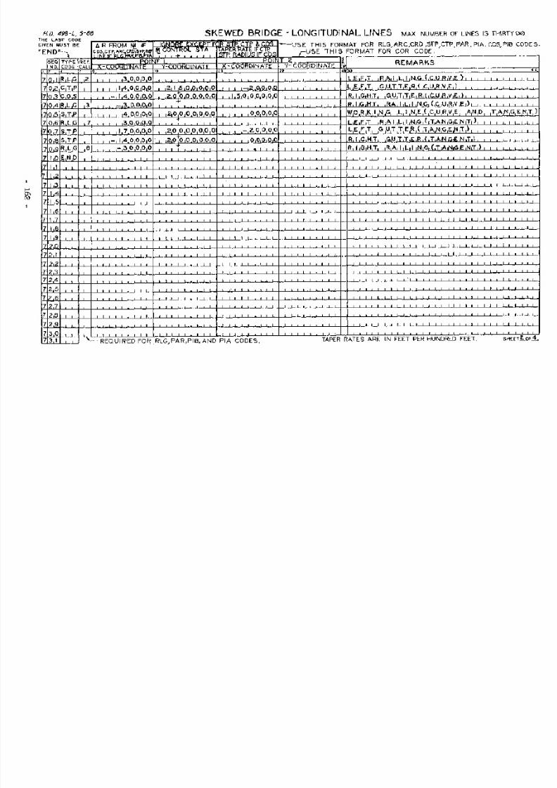
7/21/2019 Georgia Skew
http://slidepdf.com/reader/full/georgia-skew 157/182
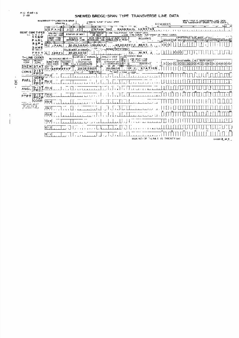
7/21/2019 Georgia Skew
http://slidepdf.com/reader/full/georgia-skew 158/182
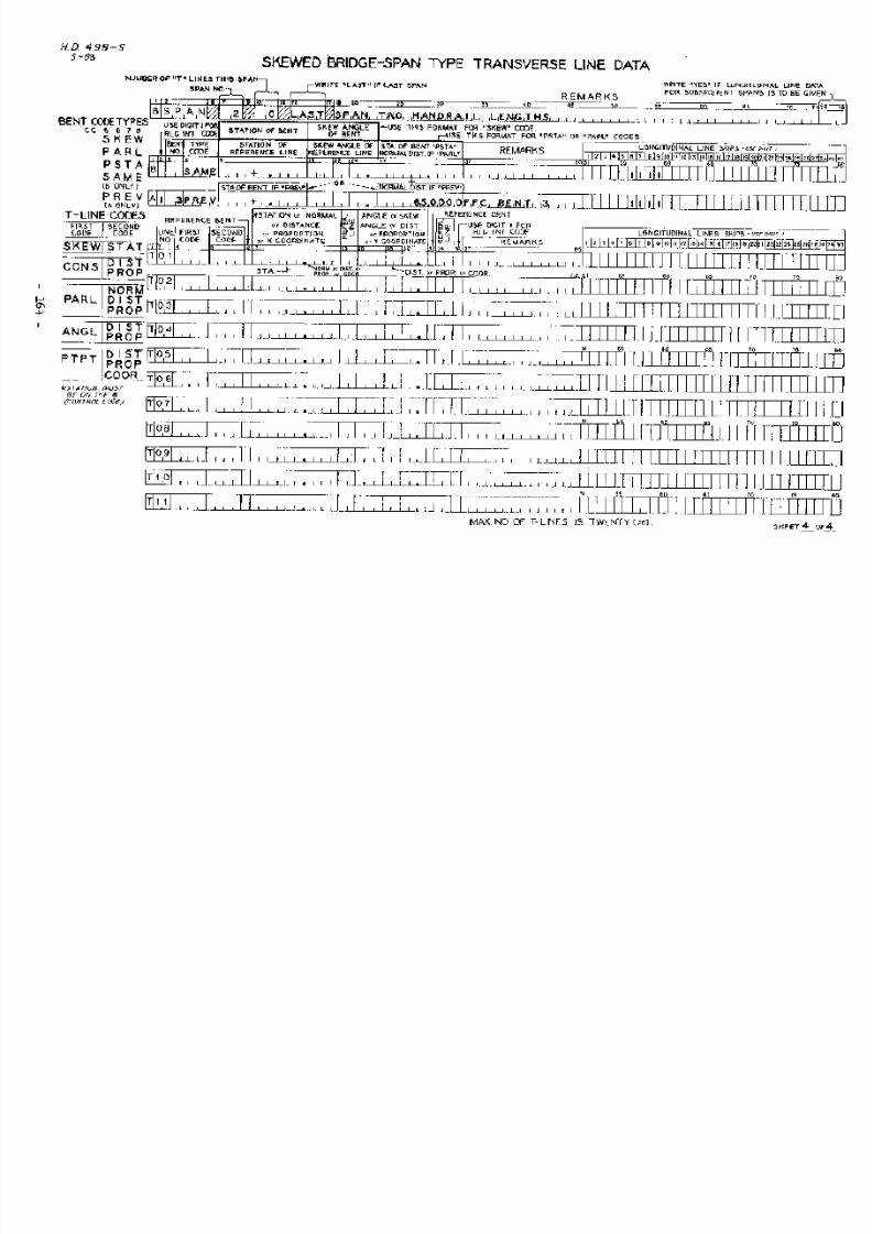
7/21/2019 Georgia Skew
http://slidepdf.com/reader/full/georgia-skew 159/182
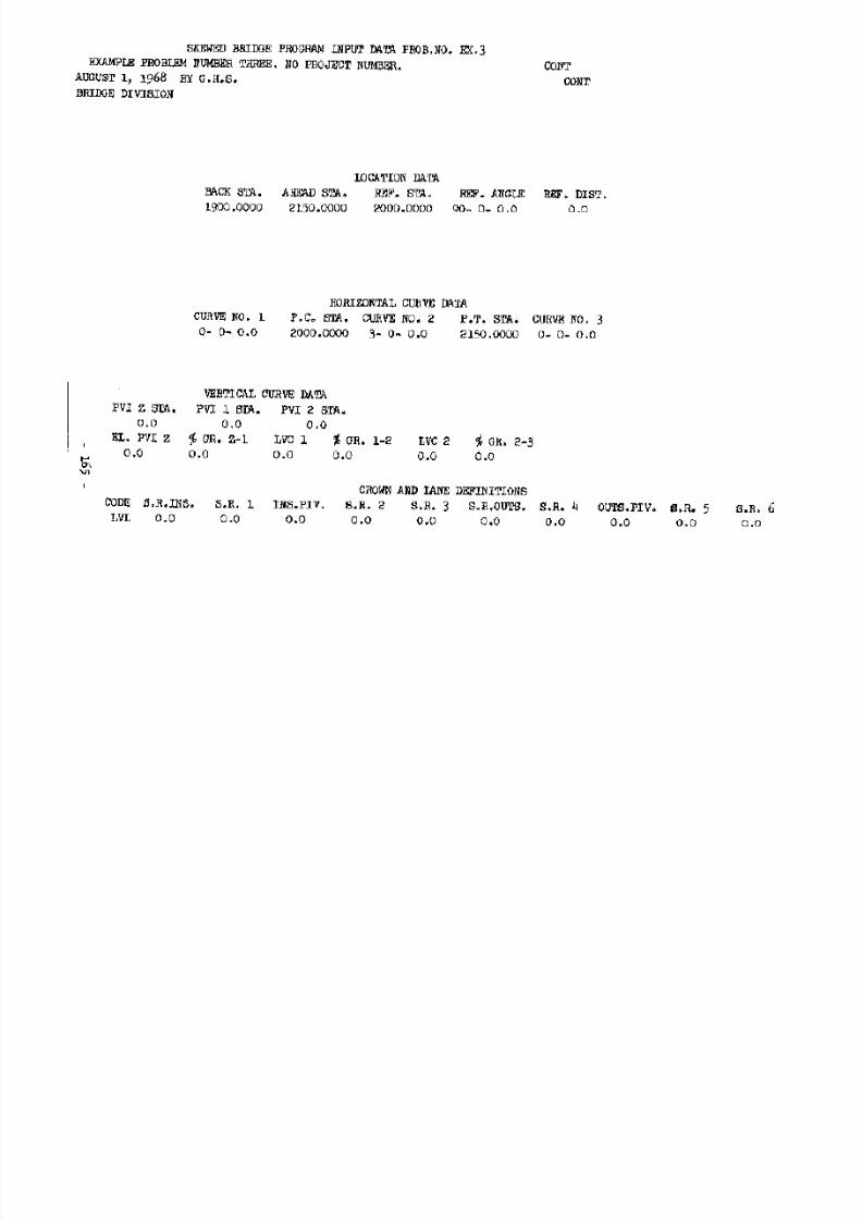
7/21/2019 Georgia Skew
http://slidepdf.com/reader/full/georgia-skew 160/182

7/21/2019 Georgia Skew
http://slidepdf.com/reader/full/georgia-skew 161/182

7/21/2019 Georgia Skew
http://slidepdf.com/reader/full/georgia-skew 162/182
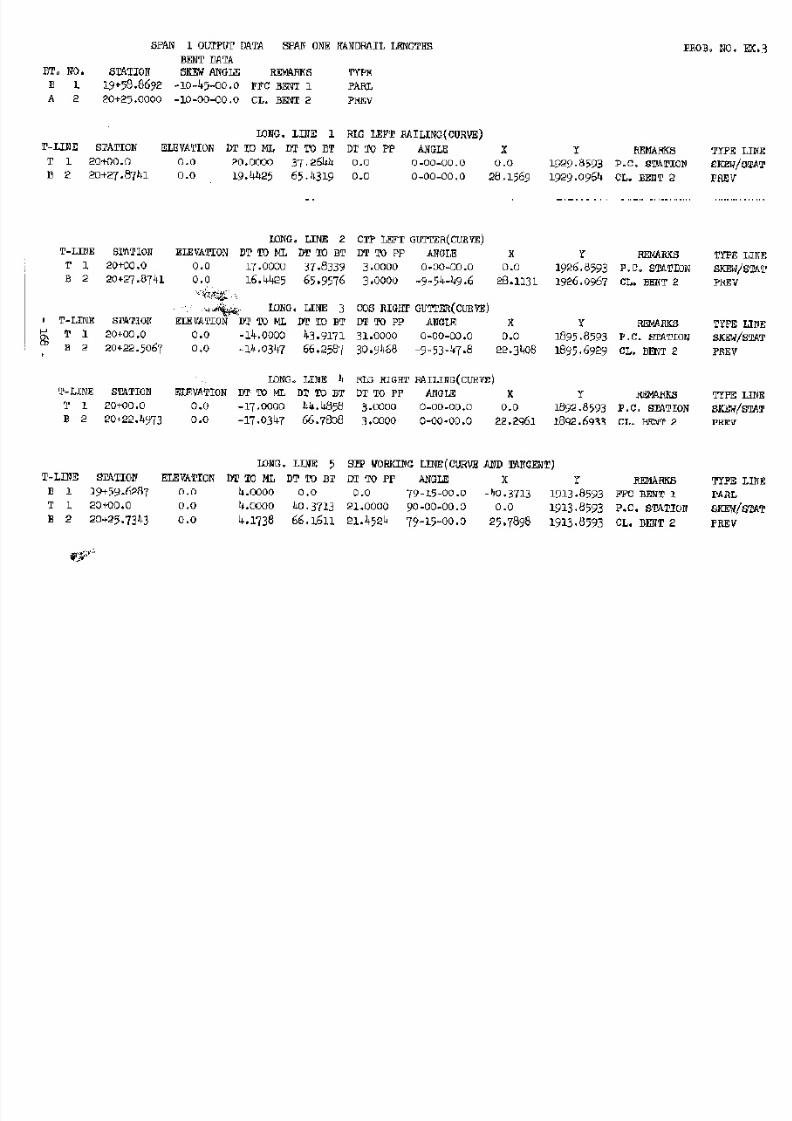
7/21/2019 Georgia Skew
http://slidepdf.com/reader/full/georgia-skew 163/182

7/21/2019 Georgia Skew
http://slidepdf.com/reader/full/georgia-skew 164/182

7/21/2019 Georgia Skew
http://slidepdf.com/reader/full/georgia-skew 165/182
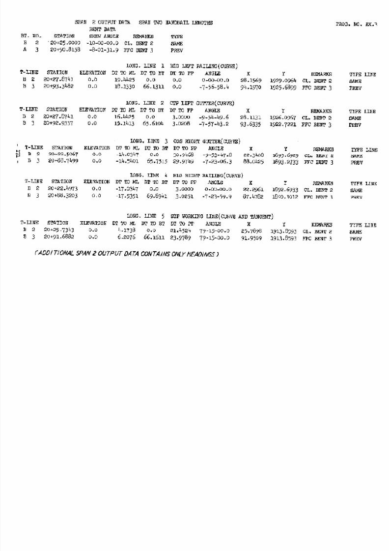
7/21/2019 Georgia Skew
http://slidepdf.com/reader/full/georgia-skew 166/182
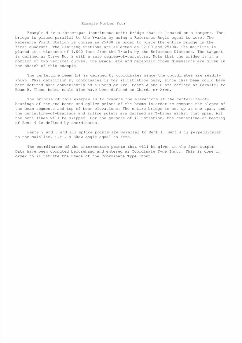
7/21/2019 Georgia Skew
http://slidepdf.com/reader/full/georgia-skew 167/182
Example Number Four
Example 4 is a three-span (continuous unit) bridge that is located on a tangent. The
bridge is placed parallel to the Y-axis by using a Reference Angle equal to zero. The
Reference Point Station is chosen as 25+00 in order to place the entire bridge in the
first quadrant. The Limiting Stations are selected as 22+00 and 25+00. The mainline is
placed at a distance of 1,000 feet from the Y-axis by the Reference Distance. The tangent
is defined as Curve No. 2 with a zero degree-of-curvature. Note that the bridge is in a
portion of two vertical curves. The Grade Data and parabolic crown dimensions are given in
the sketch of this example.
The centerline beam (B) is defined by coordinates since the coordinates are readily
known. This definition by coordinates is for illustration only, since this beam could have
been defined more conveniently as a Chord or Arc. Beams A and C are defined as Parallel to
Beam B. These beams could also have been defined as Chords or Arcs.
The purpose of this example is to compute the elevations at the centerline-of-
bearings of the end bents and splice points of the beams in order to compute the slopes of
the beam segments and top of beam elevations. The entire bridge is set up as one span, and
the centerline-of-bearings and splice points are defined as T-Lines within that span. All
the bent lines will be skipped. For the purpose of illustration, the centerline-of-bearing
of Bent 4 is defined by coordinates.
Bents 2 and 3 and all splice points are parallel to Bent 1. Bent 4 is perpendicular
to the mainline, i.e., a Skew Angle equal to zero.
The coordinates of the intersection points that will be given in the Span Output
Data have been computed beforehand and entered as Coordinate Type Input. This is done in
order to illustrate the usage of the Coordinate Type-Input.
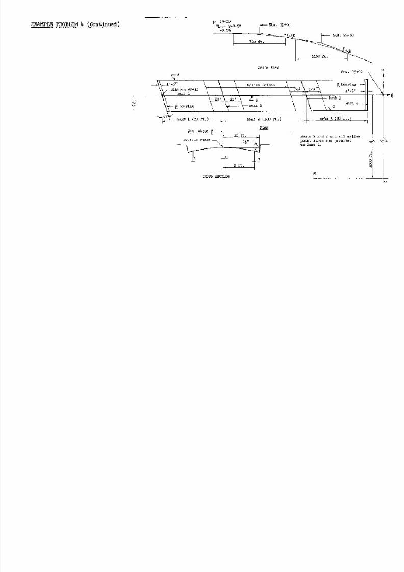
7/21/2019 Georgia Skew
http://slidepdf.com/reader/full/georgia-skew 168/182
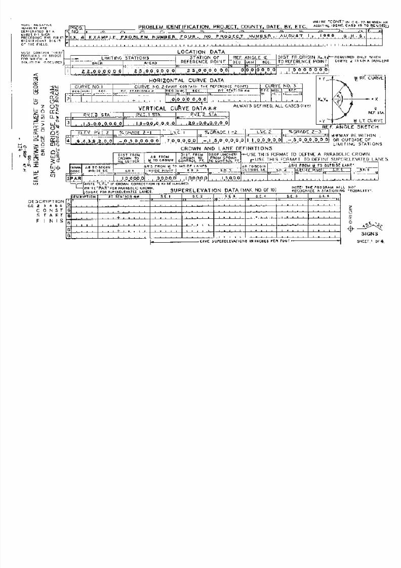
7/21/2019 Georgia Skew
http://slidepdf.com/reader/full/georgia-skew 169/182
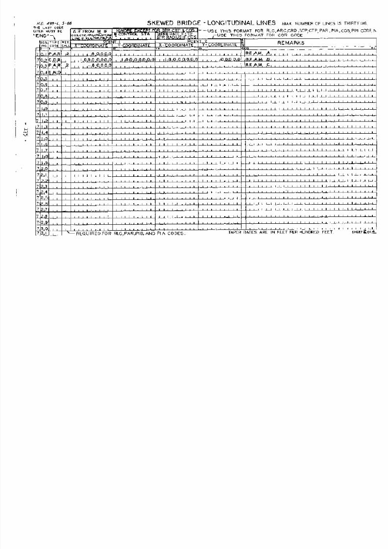
7/21/2019 Georgia Skew
http://slidepdf.com/reader/full/georgia-skew 170/182
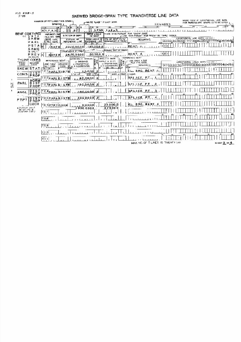
7/21/2019 Georgia Skew
http://slidepdf.com/reader/full/georgia-skew 171/182
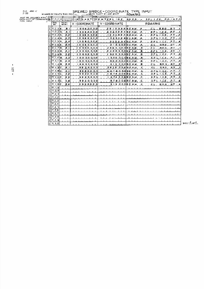
7/21/2019 Georgia Skew
http://slidepdf.com/reader/full/georgia-skew 172/182
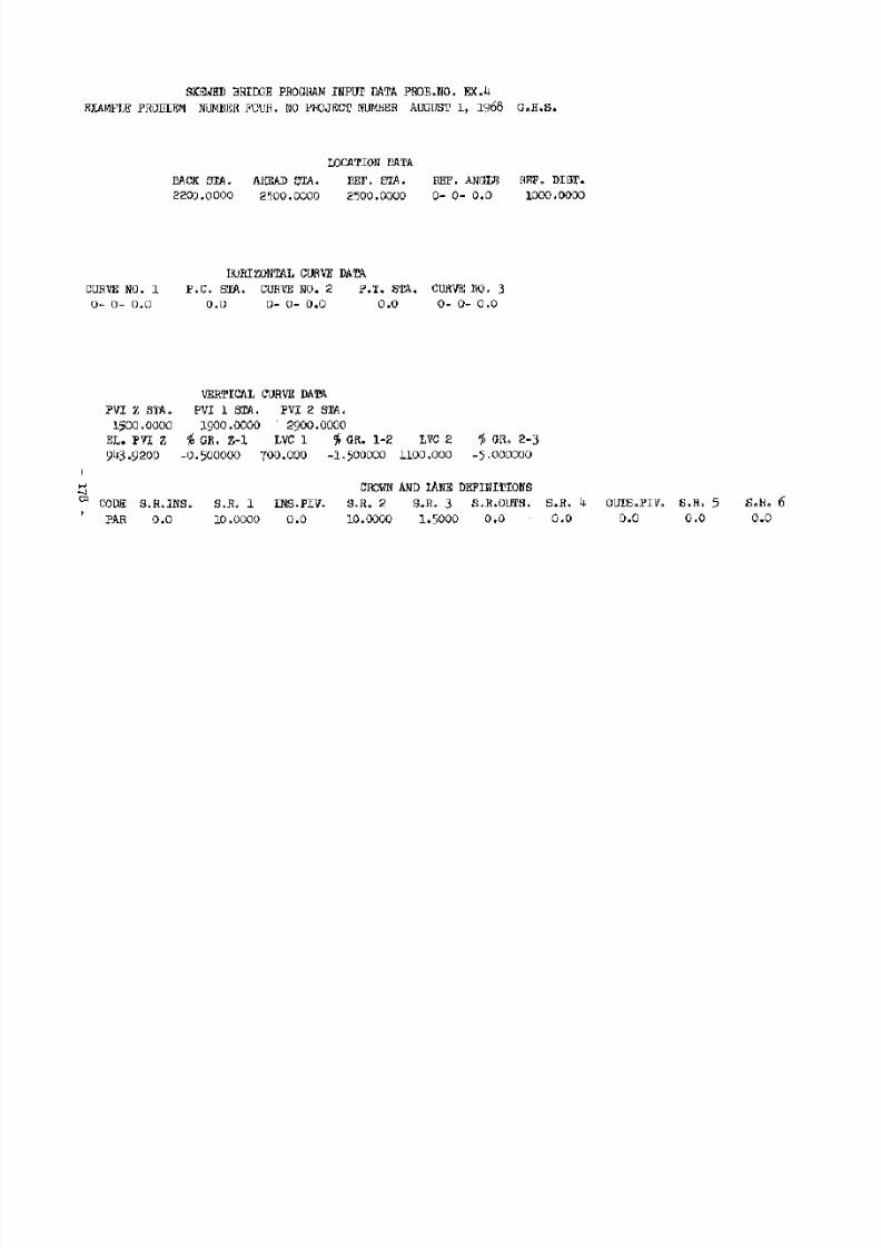
7/21/2019 Georgia Skew
http://slidepdf.com/reader/full/georgia-skew 173/182

7/21/2019 Georgia Skew
http://slidepdf.com/reader/full/georgia-skew 174/182
I
t4i
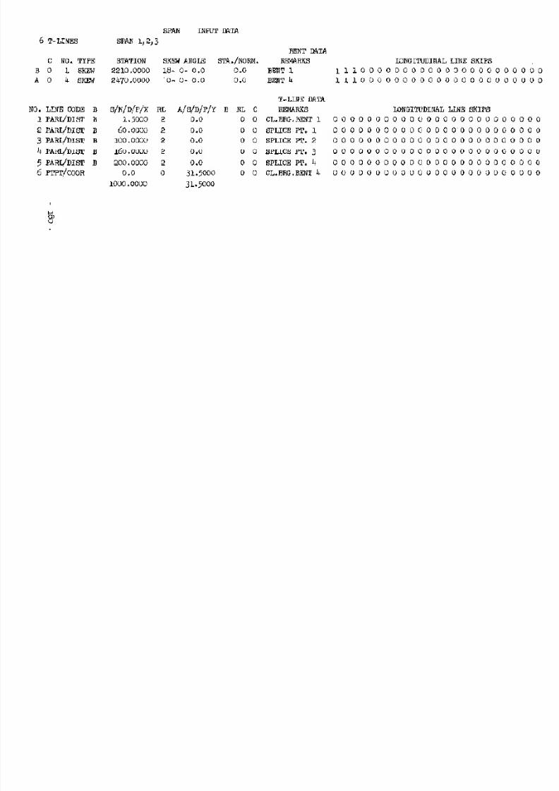
7/21/2019 Georgia Skew
http://slidepdf.com/reader/full/georgia-skew 175/182
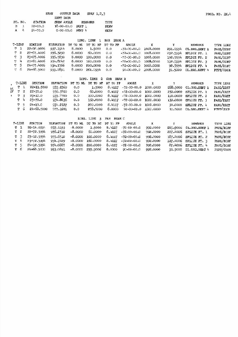
7/21/2019 Georgia Skew
http://slidepdf.com/reader/full/georgia-skew 176/182
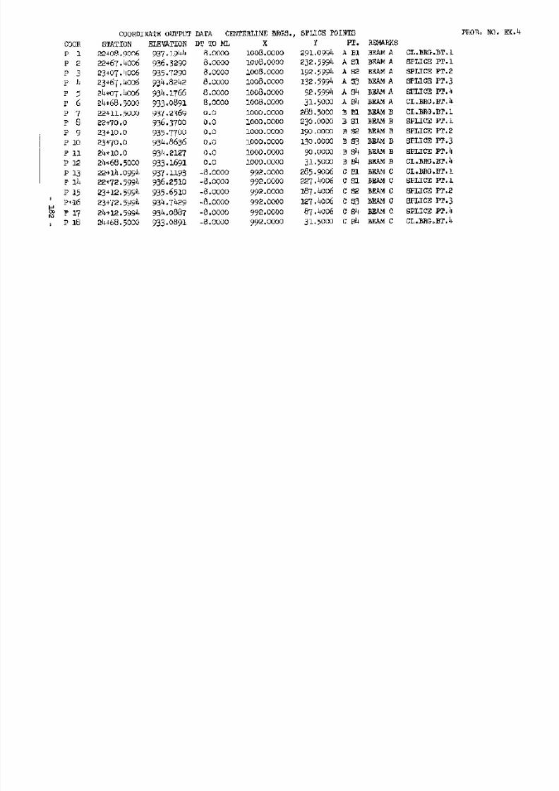
7/21/2019 Georgia Skew
http://slidepdf.com/reader/full/georgia-skew 177/182
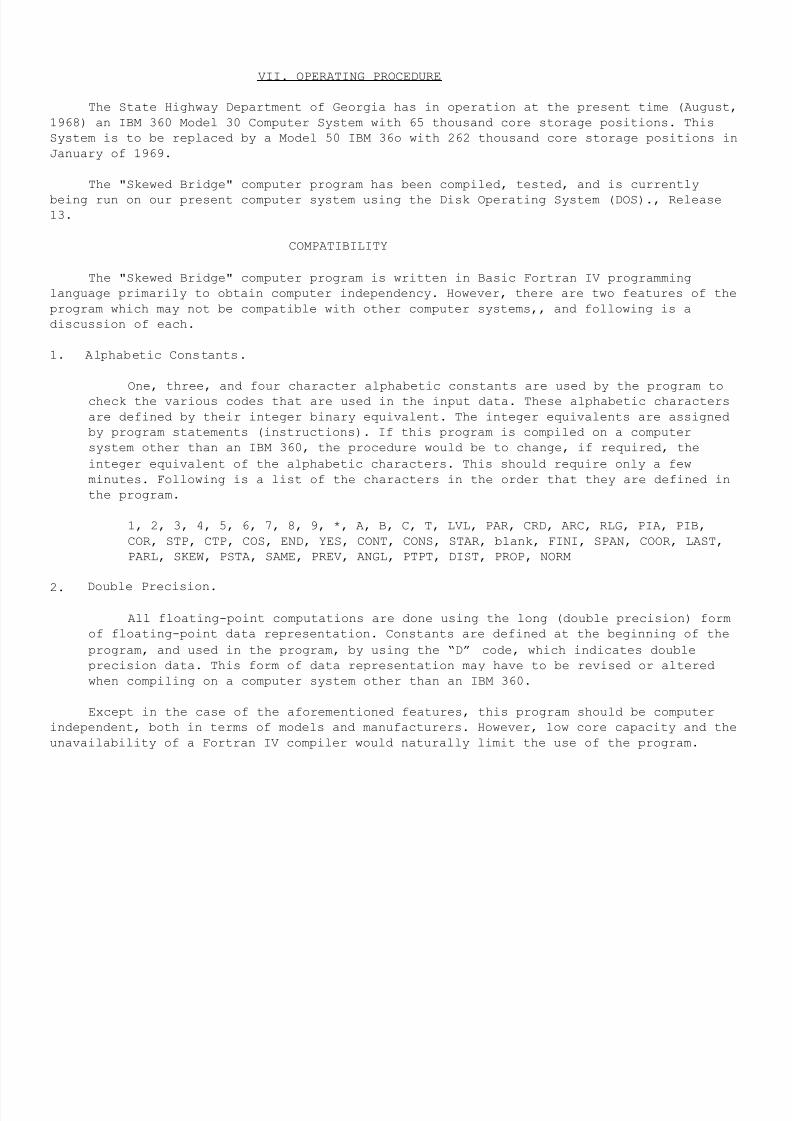
7/21/2019 Georgia Skew
http://slidepdf.com/reader/full/georgia-skew 178/182
VII. OPERATING PROCEDURE
The State Highway Department of Georgia has in operation at the present time (August,
1968) an IBM 360 Model 30 Computer System with 65 thousand core storage positions. This
System is to be replaced by a Model 50 IBM 36o with 262 thousand core storage positions in
January of 1969.
The "Skewed Bridge" computer program has been compiled, tested, and is currently
being run on our present computer system using the Disk Operating System (DOS)., Release
13.
COMPATIBILITY
The "Skewed Bridge" computer program is written in Basic Fortran IV programming
language primarily to obtain computer independency. However, there are two features of the
program which may not be compatible with other computer systems,, and following is a
discussion of each.
1. Alphabetic Constants.
One, three, and four character alphabetic constants are used by the program to
check the various codes that are used in the input data. These alphabetic characters
are defined by their integer binary equivalent. The integer equivalents are assigned
by program statements (instructions). If this program is compiled on a computer
system other than an IBM 360, the procedure would be to change, if required, the
integer equivalent of the alphabetic characters. This should require only a few
minutes. Following is a list of the characters in the order that they are defined in
the program.
1, 2, 3, 4, 5, 6, 7, 8, 9, *, A, B, C, T, LVL, PAR, CRD, ARC, RLG, PIA, PIB,
COR, STP, CTP, COS, END, YES, CONT, CONS, STAR, blank, FINI, SPAN, COOR, LAST,
PARL, SKEW, PSTA, SAME, PREV, ANGL, PTPT, DIST, PROP, NORM
2. Double Precision.
All floating-point computations are done using the long (double precision) form
of floating-point data representation. Constants are defined at the beginning of the
program, and used in the program, by using the “D” code, which indicates double
precision data. This form of data representation may have to be revised or altered
when compiling on a computer system other than an IBM 360.
Except in the case of the aforementioned features, this program should be computer
independent, both in terms of models and manufacturers. However, low core capacity and the
unavailability of a Fortran IV compiler would naturally limit the use of the program.
7/21/2019 Georgia Skew
http://slidepdf.com/reader/full/georgia-skew 179/182
COMPILING THE PROGRAM
The "Skewed Bridge" computer program, which is written in Basic Fortran IV
programming language, is divided into two parts: a Mainline program which is referred to
as Phase I, and a Subroutine which is referred to as Phase II. This division was
necessitated by the 500 statement number limitation of the Fortran IV computer (COS
Release 13). The Mainline or Phase I program CALLS the Subroutine or Phase II portion of
the program.
The core storage requirements are approximately 58,000 positions (bytes) which does
not include any supervisor program. This capacity plus the supervisor require almost the
entire core storage of a 65k computer. If the program is going to be used on a computer
system with less than 65k core storage, the program could be divided into individual
program phases. Then, a master program could be written to call and overlay the different
phases as required by the computations. If the computer system has a sufficiently large
core storage capacity, the compilation process will consist simply of compiling the
Mainline (PH. I) and Subroutine (PH. II), linkage-editing, and cataloging the program into
the systems library (core image and/or relocatable) with an appropriate name. Following is
the sequence of the Control Cards and source decks that is used when compiling, linkage-
editing, and cataloging (core image library) the program under the Disk Operating System.
// JOB SKEWBR
//OPTION CATAL
PHASE SKEWBR,*
//EXEC FORTRAN
Source Deck (PH. I)
/*
//EXEC FORTRAN
Source Deck (PH. II)
/*
// EXEC LNKEDT
/&
Note that the name "SKEWBR" has been chosen for the program; however, the name
assigned to the program is immaterial. The name of the program is left to the user's
prerogative.
7/21/2019 Georgia Skew
http://slidepdf.com/reader/full/georgia-skew 180/182
KEY-PUNCH INSTRUCTIONS
The input data will consist of several input sheets per problem with each line of the
input data sheets representing a card. The numbers of the card columns are given in the
headings of the various types of input lines for reference during and after punching. Note
that the position of the decimal that is shown on the input form does not occupy a card
column and should not be punched. However, on occasions a decimal will be entered in a
card column and, in this instance, the decimal should be punched. Plus signs (+) are in-
cluded in some of the input data. However, these signs do not occupy a card column and
should not be punched. Care should be taken to prevent the overlooking of a minus sign (a
dash) in the input data fields.
All blank data fields or card columns may be punched as zeros except in the
alphabetic fields. These data fields are read as alphabetic characters and, therefore, a
blank or zero would have a significant meaning. In addition, zeros should not be punched
in a data field immediately preceding a minus sign of that field. In general, the input
data should be punched exactly as given on input data forms. Following are examples of how
the input data is most likely to be entered in the input data fields and how the data
fields may be punched.
Only the lines that contain data entered by hand (data that is not a part of the green ink
of the input data form) should be punched. The input data should be punched in the same
sequence as given on the input data forms. That is, the key-punch operator should punch
the input data in the same sequence that it is received. Any exception to this will be
clearly noted on the input forms by the Engineer. On occasions, input data will be entered
on the forms between the input data lines. In this case, punch the data in the sequence
given as if the space between the input lines was another input line.
7/21/2019 Georgia Skew
http://slidepdf.com/reader/full/georgia-skew 181/182
COMPUTER OPERATOR INSTRUCTIONS
No instructions on the manual operation of the computer will be given here. The
computer operator is assumed to be fully versed on the computer operation. Primarily, this
discussion will present the characteristics of the program which the computer operator isrequired to know in order to process the program.
The input data (cards) should be received from the key-punch section in the correct
sequence, i.e., there should be no reason to rearrange the sequence of the input data
cards. All input data to the program is from punched cards, and all output from the
program is listed by the printer. No other I/0 devices are used. The program has the
ability to process one or several problems requiring only one EXECute Control Card with
the first problem, i.e., the program automatically continues from one problem to another.
The output form is automatically skipped by the program before printing the output data of
each problem. The output data will consist of from three to several sheets per problem.
The running time required per problem will vary depending on the amount and type of input
data with the average problem requiring approximately one and one-half minutes. The input
data cards should be entered in the card reader device in the following order:
1. // JOB SKEWBR (Job Control Card)
2. // EXEC SKEWBR (Execute Control Card)
3. Input data for all problems (Input data cards)
4. 9 ( "Last Card" Control Card to Program)
5. /* (End of Data Control Card)
6./& (End of Job Control Card)
All Control Cards except the "Last Card" Control Card are dependent on the operating
system. The Control Cards shown above are for the IBM Disk Operating System. The "Last
Card” Control Card is used by the program to indicate the end of the last problem and to
transfer control to the Supervisor. This type of Control Card makes it possible for the
program to read out all the remaining cards of a problem when an error is detected and
proceed to the next problem. The "Last Card" Control Card should have a nine (9) in card
column one (1) with all other card columns left blank.
After completing the processing of all problems, separate the output data of the
various problems and return the output data along with the input data forms to the
Engineer. The first line of output of each problem will contain:
"SKEWED BRIDGE PROGRAM INPUT DATA PROB. NO. XXXX"
where XXXX is the Problem Number which is given in card columns 2-5 of the Identification
card of the Layout Data (first sheet of each problem). This will be of assistance when
separating the output data of the various problems.

7/21/2019 Georgia Skew
http://slidepdf.com/reader/full/georgia-skew 182/182
The program has a procedure for checking the validity of the input data, and will
print an error message after detecting an error in the input data. The error message will
be given in the list of the output data of the problem in error. After an error the rest
of that problem's input data cards are read out and the program proceeds to the next
problem. Actually, the only way the computer operator will know that an error has been
detected is to observe the output data.
The procedure after an error message is to first, check the input data cards of the
problem in error for key-punch errors, and second, check the sequence of the input data
cards. If the input data cards are found to be punched correctly and in the proper
sequence, return the output data with the error message and input data forms to the
Engineer; if not, make the appropriate correction and rerun the problem from the
beginning.