Honors Abstract Algebra

Course NotesMath 55a, Harvard University

Contents

1 Introduction . . . . . . . . . . . . . . . . . . . . . . . . . . . . 12 Set Theory . . . . . . . . . . . . . . . . . . . . . . . . . . . . . 23 Vector spaces . . . . . . . . . . . . . . . . . . . . . . . . . . . 44 Polynomials . . . . . . . . . . . . . . . . . . . . . . . . . . . . 85 Linear Operators . . . . . . . . . . . . . . . . . . . . . . . . . 96 Inner product spaces . . . . . . . . . . . . . . . . . . . . . . . 167 Bilinear forms . . . . . . . . . . . . . . . . . . . . . . . . . . . 248 Trace and determinant . . . . . . . . . . . . . . . . . . . . . . 289 Introduction to Group Theory . . . . . . . . . . . . . . . . . . 3410 Symmetry . . . . . . . . . . . . . . . . . . . . . . . . . . . . . 3811 Finite group theory . . . . . . . . . . . . . . . . . . . . . . . . 5112 Representation theory . . . . . . . . . . . . . . . . . . . . . . 5513 Group presentations . . . . . . . . . . . . . . . . . . . . . . . 6514 Knots and the fundamental group . . . . . . . . . . . . . . . . 69

1 Introduction

This course will provide a rigorous introduction to abstract algebra, includinggroup theory and linear algebra.

Topics include:

1. Set theory. Formalization of Z,Q,R,C.

2. Linear algebra. Vector spaces and transformations over R and C. Otherground fields. Eigenvectors. Jordan form.

3. Multilinear algebra. Inner products, quadratic forms, alternating forms,tensor products, determinants.

4. Abstract groups.

5. Groups, symmetry and representations.

1

2 Set theory

Halmos reading. Read Halmos, Naive Set Theory, sections 1–15 to learnthe foundations of mathematics from the point of view of set theory, andits use in formalizing the integers. Most of this should be review, althoughthe systematic use of a small set of axioms to rigorously establish set theorymay be new to you. We will also formalize the rational, real and complexnumbers.

Then read 22-23 to learn about cardinality and countable sets.Finally, read 16–21 and 24–25 to learn about other versions of the axiom

of choice, ordinals and cardinals.

Axioms.

1. (Extension.) A = B iff they have the same elements.

2. (Specification.) {x ∈ A : P (x)} exists.

3. (Pairs.) {A,B} exists.

4. (Union.)⋃A exists.

5. (Infinity.) N exists. (A set containing zero and closed under n + 1 =n ∪ {n}).

6. (Power set.) P(A) exists.

7. (Axiom of Choice.) There exists a choice function c : P(A)−{∅} → Asuch that c(A) ∈ A.

8. (Well-foundedness.) There is no infinite sequence x1 ∋ x2 ∋ x3 . . ..

9. (Replacement.) If f(x) is a function defined by a logical expression,and A is a set, then f(A) is a set.

Power set and algebra. It is useful to introduce the ring Z/n (also asan example of an equivalence relation). Then we have a natural bijectionbetween P(A) and (Z/2)A. But the latter space is a ring! Note that +becomes symmetric difference, while ∗ is just intersection.

If f : A → B is a map, then we get a natural map f−1 : P(B) → P(A).This respects the ring operations. Note that E 7→ f(E) respects some butnot all! Of course if f is a bijection, it gives an isomorphism.

2

Cardinality. We write |A| = |B| if there is a bijection f : A → B. Aset is finite if |A| = |n| for some n ∈ N. This n is unique and is called thecardinality of A.

Finite sets satisfy the pigeon-hole principle: a map f : A → A is 1 − 1iff it is onto. Infinite sets are exactly the sets which do not (Hilbert’s Hotel).Using AC, one can show that any infinite set contains a copy of N, and thenn 7→ n+ 1 is 1-1 but not onto.

A set A is countable if it is finite or |A| = |N|. Note that N2 is countable;you can then show Nn is countable for all n. Similarly a countable union ofcountable sets is countable. For examples, Z[x] is countable.

On the other hand, R is uncountable (diagonalization). So we see thereare (at least) 2 kinds of infinity! This also gives a proof that:

There exists a transcendental number.

This proof is somewhat nonconstructive. An explicit such number is alsoeasy to give, e.g.

∑1/10n!.

Let us also say |A| ≤ |B| if there is an injective map f : A → B. Usingthe Axiom of Choice, we find:

If g : B → A is surjective, then there exists an injective mapf : A→ B.

(Note: although |0| < |1|, there is no surjective map 1 → 0.)

Theorem 2.1 We have |P(A)| > |A|.

Proof. Clearly A → P(A) so |P(A)| ≥ |A|. To show |P(A)| is strictlybigger, suppose f : A → P(A) is a surjection, and let B = {a ∈ A : a 6∈f(a)}. Then we cannot have B = f(a), for if we did, then a ∈ B ⇐⇒ a ∈f(a) ⇐⇒ a 6∈ f(a).

Question. (CH) Is there a set with |N| < |A| < |P(N)|? This famousproblem — the continuum hypothesis — is now know to have no solution.

(How can you prove something cannot be proved? Compare the parallelpostulate, and the axiom of infinity. Note that you need to assume yourexisting assumptions are consistent.)

Theorem 2.2 (Schroder–Bernstein) If |A| ≤ |B| and |B| ≤ |A|, then|A| = |B|.

3

Proof. We may assume A and B are disjoint. Let C = A ∪ B. ThenF = f ∪ g : C → C is injective. By following F backwards, we can partitionC into three sets: C∞ =

⋂f i(C), those with an infinite chain of ancestors;

CA = those born in A, and CB = those born in B. Taking intersection withA, we get a bijection h : A → B by setting h(x) = f(x) for x ∈ A ∩ CA,setting h(x) = g−1(x) for x ∈ A∩CB, and setting h(x) = f(x) for x ∈ A∩C∞.

Theorem 2.3 The Axiom of Choice is equivalent to the assertion that everyset can be well-ordered.

Proof. If (A,<) is well-ordered, we can define c(B) to be the least elementof B.

For the converse, let c be a choice function for A. Let us say a well-ordering (B,<) of a subset of A is guided by c if for all x ∈ B, we havex = c(A− {y ∈ B : y < x}). It is easy to see that if orderings on B and B′

are both guided by c, then B ⊂ B′ or vice-versa, and the orderings agree onB ∩ B′. Taking the union of order relations compatible with c, we obtain awell-ordering of A.

3 Vector spaces

Axler reading. We will discuss groups, rings, fields, and vector spaces overarbitrary fields. Our main text Axler [Ax] discusses only the fields R and C.For more general definitions, see [Ar, Ch. 2,3].

Note also that Axler discusses the direction sum S ⊕ T of two subspacesof a given vector space V . In general one also uses the same notation, S⊕T ,to construct a new vector space from two given ones, whose elements areordered pairs (s, t) ∈ S × T with the obvious coordinate-wise operations.

Groups and fields. An abelian group is a set G with an operation +and an element 0 such that for all a, b, c ∈ G, 0 + a = a, a + b = b + a,a + (b + c) = (a + b) + c, and there exists an element d (denoted −a) suchthat a+ d = 0.

A field K is a set with two operations, plus and times, such that (K,+)is an abelian group with identity 0, and (K∗, ·) is an abelian group withidentity 1 (where K∗ = K − {0}), and a(b+ c) = ab+ ac.

4

Note that under plus, N is not a group but Z is. Times makes Q, R andC into fields, but not Z.

Finite fields. When p is a prime, the ring Z/p is actually a field (usuallydenoted Fp). It is the unique field (up to isomorphism) containing p elements.

To see Z/p is a field, just note that if xy = 0 mod p then p|xy, which (byunique factorization) means p|x or p|y, and hence x = 0 or y = 0 modp. Soif x 6= 0, the map Z/p → Z/p given by y 7→ xy is 1 − 1. By the pigeonholeprinciple, it is onto, so there is a y such that xy = 1 mod p.

Inversion in Fp can be carried out by the Euclidean algorithm. For ex-ample, to compute 1/10 in F37, we write 37 = 3 · 10 + 7, 10 = 7 · 1 + 3,7 = 2 · 3 + 1, and then back substitute:

1 = 7−2·3 = 7−2·(10−7) = 3·7−2·10 = 3·(37−3·10)−2·10 = 3·37−11·10;

and thus 1/10 = 11 mod 37.The Euclidean algorithm can be conceived of geometrically as using a

small ruler to measure a big one and create a still smaller ruler with theremainder. If one starts with the two sides of a golden rectangle, the processnever ends. In this way the Greeks (including the secretive Pythagoreans)knew the existence of irrational numbers.

Vector spaces. A vector space over a field K is an abelian group (V,+)equipped with a multiplication mapK×V → V such that (α+β)v = αv+βv,(αβ)v = α(βv), and (especially!) 1v = v.

Examples: K, Kn. The reals form a vector space over Q.

Matrices. The n×n matrices Mn(K) with entries in a field K form a vectorspace under dimension. It looks just like Kn2

. More important, they form aring; they can be multiplied by the usual rule

(ab)ij =n∑

k=1

aikbkj .

The study of this ring will be central to the theory of vector spaces.We will later show that GLn(K), the group of matrices with nonzero

determinant, is a group under multiplication. For n = 2 this is easy: we have

(a b

c d

)−1

=1

ad− bc

(d −b−c a

)·

5

This group is (for n > 1) never commutative, e.g. a = ( 1 10 1 ) and b = ( 1 0

1 1 )satisfy

ab = ( 2 11 1 ) , ba = ( 1 1

1 2 ) .

(Although there is a field where 2 = 0, there is no field where 2 = 1!)

R4. It is sometimes useful to appreciate the geometry and topology of higher-dimensional vector spaces. Here is an example. In R2, a circle can ‘enclose’a point. The two objects are linked. But in R3 you can move the point outof the plane and then transport it to the outside of the circle, without evercrossing it.

As a test of visualization: show that two circles which are linked in R3

can be separated in R4.

Linear interdependence. A basic feature of linear dependence is the fol-lowing. Suppose

0 =n∑

1

aixi,

and all ai 6= 0. (One might then say the xi are interdependent). Then thespan of (x1, . . . , xi, . . . , xn) is the same as the span of (x1, . . . , xn), for all i.In other words, any one of the xi can be eliminated, without changing theirspan.

From this we get the main fact regarding bases.

Theorem 3.1 Let A be a linear independent set and B a finite spanning setfor a vector space V . Then |A| ≤ |B|.

Proof. Write Ai = (a1, . . . , ai) (so A0 = ∅). We inductively construct asequence of spanning sets of form Ai ∪ Bi, as follows. Let B0 = B; thenA0 ∪ B0 spans. Assuming Ai ∪ Bi spans, we can express ai+1 as a linearcombination of elements in Ai ∪ Bi. These interdependent vectors mustinclude at least one from Bi, since A is an independent set. Thus we canremove one element of Bi, to obtain a set Bi+1 such that Ai+1 ∪ Bi+1 stillspans. Note that |Bi| = |B| − i.

The induction can proceed until i reaches the minimum n of |A| and |B|.If n = |B| < |A| then Bn = ∅, while An is a proper subset of A that spansV . This contradicts the linear independence of A. Thus |B| ≥ |A|.

6

Assuming V is finite-dimensional, we obtain:

Corollary 3.2 Any linearly independent set be extended to a basis.

Corollary 3.3 All bases have the same number of elements.

When applied to the case where A and B are both bases, the proof givesmore: it gives a sequence of bases Ai∪Bi that interpolates between A and B.This can be expressed as a factorization theorem for general automorphismsof V .

Dimension. If V is a finite-dimensional vector space, we define dimV to bethe number of elements in a basis. We have just shown dimV is well-defined.

An isomorphism between vector space is a bijection map T : V1 → V2

such that T (x + y) = T (x) + T (y) and T (λx) = λT (x). It is easily verifiedthat T−1 is also an isomorphism.

Theorem 3.4 Any finite-dimensional vector space over K is isomorphic toKn for a unique n.

Note that there may be many different isomorphisms T : Kn → V . Infact, an isomorphism is the same as a choice of basis for V . Thus for any twobases (ei), (fi) of V , there is a unique isomorphism T : V → V such thatT (ei) = fi.

More generally, a linear independent set (ei)n1 for V is the same as the

choice of an injective linear map T : Rn → V , defined by T (x) =∑xiei; the

the choice of a spanning set is the same as the choice of a surjective linearmap T : Rn → V .

Infinite-dimensional vector spaces. Here is a result that conveys thepower of the Axiom of Choice.

Theorem 3.5 Any vector space V has a basis. For example, R has a basisas a vector space over Q.

Proof. Choose a well-ordering < for V (using the Axiom of choice). Let Sbe the set of v ∈ V such that v is not in the linear span of {w ∈ V : w < v}.It is easy to see that the elements of S are linearly independent. Suppose thespan S ′ of S is not all of V . Then, by well-ordering, there is a least elementv ∈ V − S ′. But then v =

∑n1 aivi with vi < v, else we would have v ∈ S.

And each vi lies in S ′, since vi < v. But then v ∈ S ′.

7

Theorem 3.6 There is a map f : R → R satisfying f(x+ y) = f(x)+ f(y),f(x) = 0 if x is rational, and f(

√2) = 1.

Proof. Let B0 = {1,√

2}. Using a small variation of the proof above, wecan extend B0 to a basis B for R over Q. Then any x ∈ R can be writtenuniquely as x =

∑B xb · b with xb ∈ Q and xb = 0 for all but finitely many

b ∈ B. This implies (x+ y)b = xb + yb. Now define f(x) = x√2.

4 Polynomials

The polynomials K[x] form a vector space over K. The elements of K[x] areformal sums

∑n0 aix

i where ai ∈ K. Thus the polynomials of degree d or lessform a vector space of dimension d+ 1.

Axler defines polynomials (p.10) as certain functions f : K → K, namelythose of the form f(x) =

∑n0 aix

i. This is fine for fields like Q and R,but it is not the right definition in general. For example, if K = Fp is thefield with p elements, there are infinitely many polynomials in Fp[x], but onlyfinitely many maps f : Fp → Fp. An important special case is the polynomialf(x) = xp−x, which vanishes for every x ∈ Fp but is not the zero polynomial.

Division of polynomials. A ratio of polynomials p/q, q 6= 0, can alwaysbe written as a ‘proper fraction’, p/q = s + r/q, where deg(r) < deg(q).Equivalently, we have:

Theorem 4.1 Given p, q ∈ K[x], q 6= 0, there exist unique polynomialss, r ∈ K[x] such that p = sq + r and deg(r) < deg(q).

Using this fact one can show that polynomials have unique factorizationinto irreducibles and have gcd’s. In particular we have this theorem:

Theorem 4.2 If p, q ∈ K[x] have no common factor, then there exist r, s ∈K[x] such that sp+ rq = 1.

Complex polynomials. We will often use:

Theorem 4.3 (Fundamental theorem of algebra) Every polynomial pin C[z] of positive degree has at least one complex zero. Thus p is a productof linear polynomials.

8

This makes it easy to see when p and q have a common factor.

Theorem 4.4 If p, q ∈ C[x] have no common zeros, then there exist r, s ∈C[x] such that sp+ rq = 1.

See [Ar, Ch. 11] for more details on polynomials.

5 Linear operators

Theorem 5.1 (Conservation of dimension) For any linear map T : V →W , we have dimV = dim KerT + dim ImT .

Proof. By lifting a basis for ImT we get a subspace S ⊂ V mappingbijectively to the image, and with V = KerT ⊕ S.

Corollary 5.2 There exists a basis for V and W such that T has the formof a projection followed by an inclusion: T : Rn → Ri ⊂ Rj.

This result shows that not only is the theory of finite-dimensional vectorspaces trivial (they are classified by their dimension), but the theory of mapsbetween different vector spaces V and W is also trivial. It is for this reasonthat we will concentrate on the theory of operators, that is the (dynamical)theory of maps T : V → V from a vector space to itself.

Rank. The dimension of ImT is also known as the rank of T . When T isgiven by a matrix, the columns of the matrix span the image. Thus the rankof T is the maximal number of linearly independent columns.

Clearly the rank of ATB is the same as the rank of T , if A and B areautomorphisms.

The row rank and the column rank of a matrix are equal. This is clearwhen the matrix of T is a projection of Rn onto Ri; it then follows from theCorollary above, by invariance of both quantities under composition withautomorphisms.

We will later see a more functorial explanation for this, in terms of vectorspaces and their duals.

The rank can be found by repeated row and/or column reduction. Rowreduction can be made into an algorithm to compute the inverse of T , as wellas a basis for the kernel when T is not invertible.

9

3

e2

1ee

Figure 1. The quotient space R3/R(1, 1, 1)

Example. Row operations on T =(

1 1 11 2 31 4 9

)lead to

(1 1 10 1 20 3 8

)and then

(1 1 10 1 20 0 2

),

showing this matrix has rank 3.

Quotient spaces. If U ⊂ V is a subspace, the quotient space V/U is definedby v1 ∼ v2 if v1−v2 ∈ U . It is a vector space in its own right, whose elementscan be regarded as the parallel translates v + U of the subspace U . There isa natural surjective linear map V → V/U . We have

dim(V/U) = dim V − dimU.

For more background see [Hal].If T ∈ Hom(V, V ) and T (U) ⊂ U then T induces a quotient map on V/U

by v + U 7→ T (v + U) + U = T (v) + U .

Exact sequences. A pair of linear maps

US→ V

T→W

is said to be exact at V if ImS = KerT . A sequence of linear maps V1 →V2 → V3 → · · · is said to be exact if it is exact at every Vi. Any linear mapT : V →W gives rise to a short exact sequence of the form

0 → Ker(T ) → VT→ Im(T ) → 0.

Block diagonal and block triangular matrices. Suppose V = A ⊕ Bwith a basis (ei) that runs first through a basis of A, then through a basis ofB.

If T (A) ⊂ A, then the matrix of T is block triangular. It has the formT =

(TAA TBA

0 TBB

). The TAA block gives the matrix for T |A. The TBB block

gives the matrix for T |(V/A). So quotient spaces occur naturally when we

10

consider block triangular matrices. Note that if S(A) = A as well, then thediagonal blocks for TS can be computed from those for S and those for T .

Finally if T (B) ⊂ B then TBA = 0 and the matrix is block diagonal. Thismeans T = (T |A) ⊕ (T |B).

Eigenvectors. Now let V be a finite-dimensional vector space over C. Aneigenvector is a nonzero vector e ∈ V such that Te = λe for some λ ∈ C,called the eigenvalue of e.

Theorem 5.3 Any linear operator T : V → V has an eigenvector.

Proof. Let n = dimV and choose v ∈ V , v 6= 0. Then the vectors(v, Tv, . . . , T nv) must be linearly dependent. In other words, there is a poly-nomial of degree n such that p(T )v = 0. Factor this polynomial; we thenhave

(T − λ1) · · · (T − λn)v = 0.

It follows that Ker(T − λi) is nontrivial for some i.

Theorem 5.4 Every operator on a finite-dimensional vector space over C

has a basis such that its matrix is upper-triangular.

Proof. Since C is algebraically closed, T has an eigenvector v1, and hencean invariant 1-dimensional subspace S = Cv1. Now proceed by induction.Consider the quotient map T : V/S → V/S. This map has a basis (v2, . . . , vn)making it upper-triangular, where vi = π(vi). Then (v1, v2, . . . , vn) put T intoupper-triangular form.

Theorem 5.5 An upper-triangular matrix is invertible iff there are no zeroson its diagonal.

Proof. If there are no zeros on the diagonal, we can in fact explicitly invertTa = b by first solving λnan = bn, and then working our way back to a1.

For the converse, suppose λi+1 = 0. Then T maps the span Vi+1 of(e1, . . . , ei+1) into Vi. So it has a nontrivial kernel.

11

Corollary 5.6 The eigenvalues of T coincide with the diagonal values ofany upper triangular matrix representing T .

Corollary 5.7 The number of eigenvalues of T is at most dimV .

Flags. A flag is an ascending sequence of subspaces, 0 = V0 ⊂ V1 ⊂ · · ·Vn =V . A flag is maximal if dim Vi = i.

Assume V is a vector space over C (or any algebraically closed field). Thetheorem on upper triangular form can be re-phrased and proved as follows.

Theorem 5.8 Any linear operator T : V → V leaves invariant a maximalflag.

Diagonalization. The simplest possible form for an operator is that itis diagonal: it has a basis of eigenvectors, Tei = λiei. Unfortunately thiscannot always be achieved: consider the operator T (x, y) = (y, 0). (Its onlyeigenvalue is zero, but it is not the zero map!) However we do have:

Theorem 5.9 If e1, . . . , em are eigenvectors for T with distinct eigenvalues,then they are linearly independent. In particular, if the number of eigenvaluesof T is equal to dimV , then T is diagonalizable.

Proof. Suppose∑m

1 aiei = 0. We can assume all ai 6= 0 and that nosmaller set of vectors is linearly dependent. But then

∑m1 λiaiei = 0, so∑m

1 (λi − λj)aiei = 0 for any j with 1 ≤ j ≤ m. This gives a smaller linearlydependent set.

Statement in terms of matrices. The preceding results show that forany T ∈ Mn(C), we can find an A ∈ GLn(C) such that ATA−1 is uppertriangular, and even diagonal if T has n distinct eigenvalues.

Generalized kernels. If T iv = 0 for some i > 0, we say v is in thegeneralized kernel of T . Since Ker(T i) can only increase with i, it muststabilize after at most n = dimV steps. Thus the generalized kernel of Tcoincides with Ker(T n), n = dimV .

Similarly we say v is a generalized eigenvector of T if v is in the generalizedkernel of T − λ, i.e. (T − λ)iv = 0 for some i. The set of all such v formsthe generalized eigenspace Vλ of T , and is given by Vλ = Ker(T − λ)n. Thenumber m(λ) = dimVλ is the multiplicity of Vλ as an eigenvalue of T .

12

Proposition 5.10 We have T (Vλ) = Vλ.

Example. Let T (x, y) = (x+ y, y). The matrix for this map, T = ( 1 10 1 ), is

already upper triangular. Clearly v1 = (1, 0) is an eigenvector with eigenvalue1. But there is no second eigenvector to form a basis for V . This is clearlyseen geometrically in R2, where the map is a shear along horizontal lines(fixing the x-axis, and moving the line at height y distance y to the right.)

However if we try v2 = (0, 1) we find that T (v2) − v2 = v1. In otherwords, taking λ = 1, v1(T − λ)v2 6= 0 is an eigenvector of T . And indeed(T − λ)2 = 0 so Vλ = V . This is the phenomenon that is captured bygeneralized eigenspaces.

Here is another way to think about this: if we conjugate T by S(x, y) =(ax, y), then it becomes T (x+(1/a)y, y). So the conjugates of T converge tothe identity. The eigenvalues don’t change under conjugacy, but in the limitthe map is diagonal.

The main theorem about a general linear map over C is the following:

Theorem 5.11 For any T ∈ HomC(V, V ), we have V = ⊕Vλ, where thesum is over the eigenvalues of V .

This means T can be put into block diagonal form, where there is onem(λ) ×m(λ) block for each eigenvalue λ, which is upper triangular and hasλ’s on the diagonal.

The characteristic polynomial. This is given by p(x) =∏

(x − λ)m(λ).Since T (Vλ) = Vλ, we have (T − λ)m(λ)|Vλ = 0. This shows:

Corollary 5.12 (Cayley-Hamilton) A linear transformation satisfies itscharacteristic polynomial: we have p(T ) = 0.

Determinants. Although we have not official introduced determinants, wewould be remiss if we did not mention that p(x) = det(xI − T ).

Lemma 5.13 If Tij is upper-triangular, then the dimension of the general-ized kernel of T (KerT n, n = dim V ) is the same as the number of zero onthe diagonal.

Proof. The proof is by induction on dimV = n. Put T in upper triangularform with diagonal entries λ1, . . . λn and invariant subspaces V1 ⊂ · · · ⊂ Vn =

13

V , with induced operators T1, . . . , Tn with ‘eventual images’ Si = ImT ni and

generalized kernels Ki. We have dimKi + dimSi = i.If λn = 0 then T (Vn) ⊂ Vn−1 so Sn = Sn−1 and hence the dimension of

the generalized kernel increases by 1. While if λn 6= 0 then Sn 6= Sn−1, sodimSn = 1 + dimSn−1 and hence the dimension of the generalized kernelremains the same.

Corollary 5.14 The dimension of Vλ coincides with the number of times λoccurs on the diagonal of Tij in upper triangular form.

Corollary 5.15 We have∑

dimVλ = dimV .

Corollary 5.16 We have V = ⊕Vλ.

Proof. Let S be the span of⋃Vλ. It remains only to show that S = V .

But since T (S) ⊂ S, if we decompose S into generalized eigenspaces, then wehave Sλ = Vλ. Thus dimS =

∑dimSλ =

∑dimVλ = dimV and so S = V .

Note that T |Vλ = λI + N where N is nilpotent. Since Nm = 0 withm = m(λ) we have

T k|Vλ =

min(k,m)∑

i=0

(k

k − i

)λk−iN i. (5.1)

Note that this is the sum of at most m terms, each of which is a polynomialin k times λk.

Spectral radius. The following result is often useful in application with adynamical flavor. Let ‖T‖ denote any reasonable measurement of the size ofT , for example sup |Tij|, such that ‖λT‖ = |λ| · ‖T‖.

Theorem 5.17 We have lim ‖T n‖1/n = sup |λ|, where λ ranges over theeigenvalues of T .

The eigenvalues of T are also known as its spectrum, and sup |λ| = ρ(T )as the spectral radius of T . This follows easily from (5.1).

14

Jordan blocks and similarity. A Jordan block is an upper triangularmatrix such as

T =

λ 1

λ 1

λ 1

λ 1

λ

(where the missing entries are zero). It has the form T = λI + N , whereN is an especially simple nilpotent operator: it satisfies N(ei) = ei−1, andN(e1) = 0.

Two operators on V are similar if ST1S−1 = T2 for some S ∈ GL(V ).

This means T1 and T2 have the same matrix, for suitable choice of bases.

Theorem 5.18 Every T ∈ Mn(C) is similar to a direct sum of Jordanblocks. Two operators are similar iff their Jordan blocks are the same.

Nilpotence. The exponent of a nilpotent operator is the least q ≥ 0 suchthat T q = 0.

By considering (T − λ)|Vλ, the proof of the existence of Jordan formfollows quickly from the nilpotent case, i.e. the case λ = 0. In this case theJordan block is a nilpotent matrix, representing the transitions a graph suchas the one shown for q = 5 in Figure 2.

Theorem 5.19 Let T be nilpotent with exponent q, and suppose v 6∈ Im(T ).Then V admits a T -invariant decomposition of the form V = A⊕ B, whereA is spanned by (v, Tv, . . . , T q−1v).

Proof. Let A0 = A and let A1 = T (A0). Note that T | Im(T ) has exponentq − 1; thus by induction we can have a T -invariant decomposition Im(T ) =A1 ⊕ B1. Let B0 = T−1(B1).

We claim that (i) A0 +B0 = V and (ii) A0 ∩B1 = (0). To see (i) supposev ∈ V ; then T (v) = a1 + b1 ∈ A1 ⊕B1 and a1 = T (a0) for some a0 ∈ A0; andsince T (v − a0) = b1 ∈ B1, we have v − a0 ∈ B0.

To see (ii) just note that B1 ⊂ Im(T ), so A0 ∩B1 = A1 ∩B1 = (0).Because of (i) and (ii) we can choose B such that B1 ⊂ B ⊂ B0 and

V = A0 ⊕ B. Then T (C) ⊂ T (B0) ⊂ B1 ⊂ C and we are done.

15

Graphs. Suppose G is a directed graph with vertices 1, 2, . . . , n. Let Tij = 1if i is connected to j, and 0 otherwise. Then (T k)ij is just the number ofdirected paths of length k that run from i to j.

Theorem 5.20 The matrix T is nilpotent if and only if T has no cycle.

Figure 2. A nilpotent graph.

Jordan canonical form: an algorithm? It is tempting to think that abasis to put a matrix into Jordan canonical form can be obtained by firsttaking a basis for the kernel of T , then by taking preimages of these baseelements, etc. This need not work! For example, we might have dim Im(T ) =1 and dim Ker(T ) = 2; then the original basis for the kernel had bettercontain an element from the image, otherwise we will be stuck after the firststage, when we are still short of a basis.

The minimal polynomial. This is the unique monic polynomial q(x) ofminimal degree such that q(T ) = 0. For example, the characteristic andminimal polynomials of the identity operator are given by p(x) = (x − 1)n

and q(x) = (x− 1). It is straightforward to verify that

q(x) =∏

(x− λ)M(λ),

where M(λ) is the exponent of (T − λ)|Vλ. This is the same as the maximaldimension of a Jordan block of T with eigenvalue λ.

Classification over R : an example.

Theorem 5.21 Every T ∈ SL2(R) is either elliptic, parabolic,or hyperbolic.

6 Inner product spaces

In practice there are often special elements in play that make it possible todiagonalize a linear transformation. Here is one of the most basic.

Theorem 6.1 (Spectral theorem) Let T ∈ Mn(R) be a symmetric ma-trix. Then Rn has a basis of orthogonal eigenvectors for T .

16

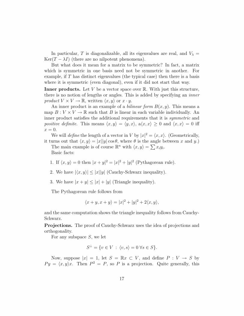
In particular, T is diagonalizable, all its eigenvalues are real, and Vλ =Ker(T − λI) (there are no nilpotent phenomena).

But what does it mean for a matrix to be symmetric? In fact, a matrixwhich is symmetric in one basis need not be symmetric in another. Forexample, if T has distinct eigenvalues (the typical case) then there is a basiswhere it is symmetric (even diagonal), even if it did not start that way.

Inner products. Let V be a vector space over R. With just this structure,there is no notion of lengths or angles. This is added by specifying an innerproduct V × V → R, written 〈x, y〉 or x · y.

An inner product is an example of a bilinear form B(x, y). This means amap B : V × V → R such that B is linear in each variable individually. Aninner product satisfies the additional requirements that it is symmetric andpositive definite. This means 〈x, y〉 = 〈y, x〉, a〈x, x〉 ≥ 0 and 〈x, x〉 = 0 iffx = 0.

We will define the length of a vector in V by |x|2 = 〈x, x〉. (Geometrically,it turns out that 〈x, y〉 = |x||y| cos θ, where θ is the angle between x and y.)

The main example is of course Rn with 〈x, y〉 =∑xiyi.

Basic facts:

1. If 〈x, y〉 = 0 then |x+ y|2 = |x|2 + |y|2 (Pythagorean rule).

2. We have |〈x, y〉| ≤ |x||y| (Cauchy-Schwarz inequality).

3. We have |x+ y| ≤ |x| + |y| (Triangle inequality).

The Pythagorean rule follows from

〈x+ y, x+ y〉 = |x|2 + |y|2 + 2〈x, y〉,

and the same computation shows the triangle inequality follows from Cauchy-Schwarz.

Projections. The proof of Cauchy-Schwarz uses the idea of projections andorthogonality.

For any subspace S, we let

S⊥ = {v ∈ V : 〈v, s〉 = 0 ∀s ∈ S}.

Now, suppose |x| = 1, let S = Rx ⊂ V , and define P : V → S byPy = 〈x, y〉x. Then P 2 = P , so P is a projection. Quite generally, this

17

implies V = KerP ⊕ ImP , as can be seen by writing y = Py + (I − P )y. Inthe case at hand, clearly KerP = S⊥. So we have V = S ⊕ S⊥.

Consider any y, and write y = Py + z where Py ∈ S and z ∈ S⊥. Thenwe have

|y|2 = |Py|2 + |z|2 ≥ |Py|2 = |〈x, y〉|2,which gives Cauchy-Schwarz. Note that equality in Cauchy-Schwarz iff y ∈Rx or x = 0.

Theorem 6.2 For any subspace S, we have V = S ⊕ S⊥.

Proof. Since S⊥ is defined by dimS linear conditions, we have dimS⊥ +dimS ≥ dimV . On the other hand, the Pythagorean rule implies the mapS ⊕ S⊥ → V has no kernel.

Corollary 6.3 There is a natural ‘orthogonal projection’ P : V → S, char-acterized by 〈y, s〉 = 〈Py, s〉 for all s ∈ S. Its kernel is S⊥.

Orthonormal bases. Let us say (ei)m1 is an orthonormal basis for S if

〈ei, ej〉 = δij and the span of (ei) is S. If S has an orthonormal basis, thenwe get an explicit formula for P :

P (v) =∑

〈v, ei〉ei.

Theorem 6.4 Any finite-dimensional inner product space has an orthonor-mal basis.

Proof. By induction on dimV . Clear if dimV ≤ 1, so assume dimV > 1.Pick any e1 ∈ V with |e1| = 1. Then (e1) is an orthonormal basis for S = Re1,so the projection to S is defined and V = S ⊕ S⊥. By induction, S⊥ has anorthonormal basis (e2, . . . , en), which together with e1 gives one for V .

Corollary 6.5 Any finite-dimensional inner product space is isomorphic toRn with the usual inner product.

18

Sequence spaces. The Cauchy-Schwarz inequality is already a powerfultool for bounded finite sums:

(∑anbn

)2

≤(∑

a2n

)(∑b2n

).

This works for infinite sums as well, and makes ℓ2(N) = {an :∑a2

n < ∞}into an inner product space. For example, we have

|∑

an/n|2 ≤ (∑

a2n)(∑

1/n2) = (π2/6)∑

a2n.

Function spaces. Another typical inner-product space is the space of poly-nomials R[x] with

〈f, g〉 =

∫ b

a

f(x)g(x) dx.

Note that the monomials (1, x, x2, . . .) form a basis for this space but not anorthonormal basis. The Gram-Schmidt process gives an inductive procedurefor generating an orthonormal basis from a basis.

Hermitian inner products. We mention that similar definitions and re-sults hold for vector spaces over C. In this setting the standard example isV = Cn with 〈x, y〉 =

∑xiyi. Note that 〈y, x〉 = 〈x, y〉 and we only have

(complex) linearity in the first coordinate. A positive-definite bilinear formwith these properties is called a Hermitian inner product.

Example: the space V = C[z, z−1] of function on the circle S1 ⊂ C thatare polynomials in z and 1/z forms a Hermitian vector space with respect tothe inner product

〈f, g〉 =1

2π

∫

S1

f(z)g(z) |dz|.

More on projections. Let P : V → S be orthogonal projection to S. Weremark that Pv is the unique point in S closest to v. To see this, recall thatt = v − Pv ∈ S⊥. So if s′ ∈ S we have

|v − s′|2 = |s− s′ + t|2 + |s− s′|2 + |t|2 ≥ |t|2 = |Pv − v|2.

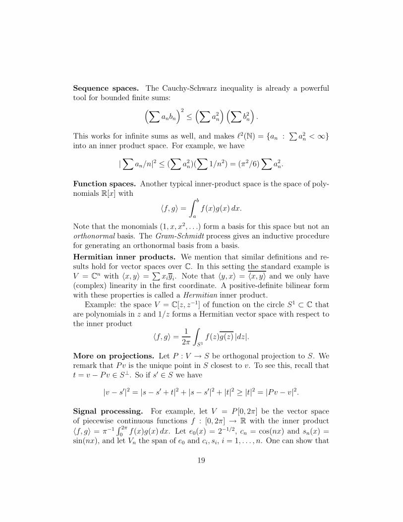
Signal processing. For example, let V = P [0, 2π] be the vector spaceof piecewise continuous functions f : [0, 2π] → R with the inner product

〈f, g〉 = π−1∫ 2π

0f(x)g(x) dx. Let e0(x) = 2−1/2, cn = cos(nx) and sn(x) =

sin(nx), and let Vn the span of e0 and ci, si, i = 1, . . . , n. One can show that

19

1 2 3 4 5 6

0.2

0.4

0.6

0.8

1.0

Figure 3. Square wave approximated by terms up to sin(9x).

this is an orthogonal basis, so it can be used to compute the projection gn off to Vn. For f(x) = 1 on [0, π] and 0 on [π, 2π] we find:

gn(x) =1

2+

k=n∑′

1

2

πksin kx,

where only odd values of k are included in the sum.

The dual space. For a more functorial discussion, we introduce the dualspace V ∗ = Hom(V,R). This is a new vector space built naturally from V ;its elements consists of linear maps or functionals φ : V → R.

Theorem 6.6 For all φ ∈ V ∗ there exists a unique y ∈ V such that φ(x) =〈x, y〉 for all x ∈ V .

Proof. Choose an orthonormal basis (ei) and let y =∑φ(ei)ei.

Corollary 6.7 We have dimV = dimV ∗.

Adjoints. Let T be a linear operator on V . Then for any y ∈ V , the mapx 7→ 〈Tx, y〉 is a linear functional on V . Thus there is a unique vector z suchthat 〈Tx, y〉 = 〈x, z〉 for all x ∈ V . We write z = T ∗(y) and use it to definea new linear operator, the adjoint of T . It satisfies

〈Tx, y〉 = 〈x, T ∗y〉

for all x, y ∈ V .

20

Theorem 6.8 Let ei be an orthonormal basis for V . Then the matrix forT ∗ with respect to (ei) is the transpose of the matrix for T .

Corollary 6.9 An operator T ∈ Mn(R) is self-adjoint iff Tij = Tji.

Note that (ST )∗ = T ∗S∗, T ∗∗ = T , and if T (S) ⊂ S then T (S⊥) ⊂ S⊥.

The spectral theorem. We can now prove that a self-adjoint operatoris diagonal with respect to a suitable orthonormal basis. In other words, ifT = T ∗ then V has an orthonormal basis of eigenvectors for T . Note thatwe are working over R, not C, and we are getting honest eigenvectors, notgeneralized eigenspaces.

The proof is based on some preliminary good properties for T . SupposeT is self-adjoint.

Lemma 6.10 If T (S) ⊂ S then T (S⊥) ⊂ S⊥.

Lemma 6.11 We have 〈v, T 2v〉 ≥ 0 for all v.

(In other words, whenever T is self-adjoint (or ‘real’), T 2 is a positiveoperator).

Corollary 6.12 If a > 0 then T 2+a is invertible. More generally, T 2+aT+bis invertible if p(x) = x2 + ax+ b has no real root.

Corollary 6.13 The operator T has a (real) eigenvector.

Proof. As usual, by considering v, Tv, . . . , T nv as find a nontrivial monicpolynomial p ∈ R[x] such that dim Ker p(T ) > 0. Now over R, p(x) factorsinto linear terms (x − ri) (with real roots) and quadratic terms qi(x) (withno real roots). By the preceding Corollary, qi(T ) is invertible for each i, so(T − riI) must be noninvertible for some i.

Proof of the spectral theorem. By induction on dimV . Let S = Re1 bethe span of a unit eigenvector. Then T (S⊥) ⊂ S⊥, and T |S⊥ has a basis ofeigenvectors by induction.

21

(Note: one should verify that T ∗(S) ⊂ S.)

The orthogonal group. The symmetries of V which preserve its innerproduct form the orthogonal group O(V ). These are exactly the linear trans-formations T such that

〈Tx, Ty〉 = 〈x, y〉for all x, y. Equivalently, we have

〈x, T ∗Ty〉 = 〈x, y〉.

But this happens iff T ∗T = I. Thus:

O(V ) = {T ∈ Hom(V, V ) : T ∗T = I}.

Equivalently, we have T−1 = T ∗. So these transformations are sort of ‘anti-self adjoint’.

The terminology is explained by the following observation: a matrix Tij

belongs to O(Rn) iff its columns form an orthonormal basis for Rn.

Example: the orthogonal group of the plane. A matrix belongs toO2(R) iff it has the form

(a −bb a

)or(

a bb −a

), with a2 + b2 = 1. The rotations

of R2 are given by T =(

cos θ − sin θsin θ cos θ

). The others give reflections.

Theorem 6.14 For any orthogonal transformation T , there exists an or-thogonal splitting V = ⊕Vi where each Vi has dimension 1 or 2. When Vi istwo-dimensional, T |Vi is a rotation; when Vi is one-dimensional, T |Vi = ±I.

Proof. Recall that every real operator has an invariant subspace V1 ofdimension one or two. This is the span of v and Tv where v is in the kernelof T −a or T 2−bT −c. Since T is an isometry, T (V1) = V1 and T (V ⊥

1 ) = V ⊥1 .

The proof then proceeds by induction.

Corollary 6.15 Every isometry of the 2-sphere that preserves its orientationis a rotation about an axis.

Interaction of orthogonal and self-adjoint transformations. Notethat if R ∈ O(V ), then (RTR−1)∗ = RT ∗R−1. In particular, the conjugateof a self-adjoint transformation by an orthogonal one is still self-adjoint.

The spectral theorem can be restated as:

22

Theorem 6.16 If T is a symmetric matrix, then there is an R ∈ On(R)such that RTR−1 is diagonal.

Polar decomposition. An operator T is positive if T = T ∗ and 〈Tv, v〉 ≥ 0for all v. This is equivalent to its eigenvalues satisfying λi ≥ 0. (Q. Is thecondition that T = T ∗ redundant?)

Proposition 6.17 A positive operator has a unique positive square-root.

Clearly A∗A is positive for any operator A.

Theorem 6.18 (Polar decomposition) Any invertible operator A on Vcan be unique expressed as A = TR, where T is positive and R ∈ On(R).

Proof. Let T =√A∗A; then R = AT−1 satisfies RR∗ = AT−2A∗ =

A(A∗A)−1A = I, so R ∈ On(R).

Functional calculus. More generally, if T = T ∗ and f : R → R is anycontinuous function, then f(T ) makes sense; and if T is positive, then fneed only be defined on [0,∞). This ‘functional calculus’ takes the obviousvalues on polynomials and satisfies fn(T ) → f(T ) if fn → f ; and f(g(T )) =(f ◦ g)(T ).

Normal operators. Here is a useful extension to a vector space V over C

equipped with a Hermitian form. We say an operator is normal if TT ∗ = T ∗T .

Theorem 6.19 A transformation T ∈ GLn(V ) has an orthonormal basis ofeigenvectors iff T is normal.

Proof. Clearly diagonal matrices are normal. For the converse, let V1 =Ker(T − λ1I) ⊂ V be a nontrivial eigenspace. We claim T and T ∗ bothpreserve the splitting V = V1 ⊕ V ⊥

1 .First, we always have T ∗(V ⊥

1 ) ⊂ V ⊥1 (whether or not T is normal). But

we also have T ∗(V1) ⊂ V1, since for v ∈ V1 we have

TT ∗(v1) = T ∗T (v1) = T ∗(λ1v1) = λ1T∗(v1).

This implies T (V ⊥1 ) ⊂ V ⊥

1 . Then T |V ⊥1 is also normal and the proof proceeds

by induction.

23

7 Bilinear forms

Let B : V × V → R be a bilinear form on a finite-dimensional real vectorspace.

We say B is degenerate if there is an x 6= 0 such that B(x, y) = 0 for all y;otherwise it is nondegenerate. Any bilinear form is the sum of a symmetricand an antisymmetric one. Our aim is to classify these.

It is often useful to give V an inner product, which we can then compareto B.

Proposition 7.1 If V has an inner product, then there is a unique operatorA such that

B(x, y) = 〈x,Ay〉.The form B is symmetric iff A is self-adjoint; antisymmetric iff A∗ = −A;and B is nondegenerate iff A is invertible.

Quadratic forms. Suppose B is symmetric. Associated to B(x, y) is thequadratic form

Q(x) = B(x, x).

The form Q determines B, since

2B(x, y) = Q(x+ y) −Q(x) −Q(y).

(Note that for an antisymmetric form, Q would be zero.)(Aside: this formula is related to the famous equation

(x2 + y2) − (x2 − y2)2 = (2xy)2,

which allows one to generate all Pythagorean triples. The geometric meaningof this equation is that the rational solutions to a2 + b2 = 1, projected from(a, b) = (0, 1), are in bijection with the rational numbers on the a-axis.)

A quadratic form on Rn is nothing more than a homogeneous quadraticpolynomial in the coordinates on Rn:

Q(x) =∑

aijxixj ,

and the coefficients aij are unique if we require aij = aji. If we say A(x) =∑aijxj , then

B(x, y) = 〈x,Ay〉.

24

Examples with mixed signatures. For the usual inner product, Q(x) =|x|2. But there are other important examples! The standard quadratic formof signature (p, q) on Rn, n ≥ p+ q, is given by

Q(x) =

p∑

1

x2i −

q∑

p+1

x2i .

This form is nondegenerate iff p+ q = n.Note that even when Q is nondegenerate, the ‘lengths’ of vectors can have

both signs, or even be zero.Another important example is provided by Q(x, y) = xy on R2. This is

in fact equivalent to the standard form of signature (1, 1). In fact, if we lete1 = (1, 1)/

√2 and e2 = (1,−1)/

√2, then B(ei, ej) = ( 1 0

0 −1 ).

Theorem 7.2 For any real quadratic form on a finite-dimensional vectorspace V , there exists a basis such that Q(x) is the standard quadratic formof signature (p, q) with p+ q ≤ n.

Proof. Choose an inner product on V and write the associated bilinear formas B(x, y) = 〈x,Ay〉 where A is self-adjoint. Then choose an orthonormalbasis ei of eigenvectors for A with eigenvalues λi. Replacing ei with |λi|−1/2ei,we can assume B(ei, ei) = ±1 or 0.

Conics and quadrics. A real quadric X ⊂ Rn is the locus defined by anequation of the form

f(x) = Q(x) + L(x) + C = 0,

where Q(x) is a quadratic form, L(x) is linear and C is a constant. We saytwo quadrics are equivalent if there is an (invertible) affine transformationT (x) = Ax + b such that T (X1) = X2. A quadric is degenerate if Q is zero,or it is equivalent to one where f does not depend on all the coordinates, orwhere the linear and constant term both vanish.

To classify nondegenerate quadrics, we first arrange that Q has signature(p, q), 1 ≤ p + q ≤ n. Then we can complete the square to eliminate all butr = n− p− q coordinates from L(x). If r > 0 then we can translate in thesecoordinates to absorb the constant. If r > 1 then we can get rid of one ofthe linear coordinates completely, so the quadric is degenerate. And if thereis no linear term, we can scale Q so the constant becomes 1. So in the endwe find:

25

Theorem 7.3 Any nondegenerate quadric is equivalent to one given by apurely quadratic equation of the form

Qpq(x) = 1,

with p + q = n, p ≥ 1; or by a parabolic equation

xn = Qpq(x),

where p ≥ q, p+ q = n− 1.

Corollary 7.4 Any nondegenerate conic is equivalent to the circle x2 +y2 =1, the hyperbola x2 − y2 = 1, or the parabola y = x2.

Theorem 7.5 Any nondegenerate quadric in R3 is equivalent to either:

1. The sphere x2 + y2 + z2 = 1; or

2. The 1-sheeted hyperboloid x2 + y2 − z2 = 1; or

3. The 2-sheeted hyperboloid x2 − y2 − z2 = 1; or

4. The elliptic paraboloid z = x2 + y2; or

5. The hyperbolic paraboloid z = x2 − y2.

Alternating forms. We now handle the alternating case.Suppose B(x, y) = −B(y, x). The main example of such a form is

B(x, y) = det

(x1 x2

y1 y2

)= x1y2 − x2y1.

This form measures the signed area of the parallelogram with sides x and y.By taking the sum of n such forms, we obtain a nondegenerate alternatingform on R2n. It is given by B(x, y) = 〈x, J2ny〉 where J2n has n blocks of theform ( 0 1

−1 0 ) on the diagonal.A nondegenerate alternating form is also called a symplectic form

Theorem 7.6 Let B(x, y) be a symplectic form on finite-dimensional realvector space V . Then dimV = 2n is even, and there exists a basis such thatB(ei, ej) = (J2n)ij.

26

Note. The prototypical example of such a form arises on the homology of aclosed orientable surface of genus g.

Proof. Choose any e1 6= 0. Then there exists an e2 such that B(e1, e2) = 1(else B is degenerate). Let V1 be the span of e1 and e2; this is 2-dimensional,else we would have B(e1, e2) = 0. The matrix of B|V1 is now J2.

Let V ⊥1 = {v ∈ V : B(v, e1) = B(v, e2) = 0}. It is easy to see that

V = V1 ⊕ V ⊥1 . First, these two subspaces meet only at 0 since B|V1 is non-

degenerate. And second, V ⊥1 is the kernel of a map to R2, so its dimension

is (at least) n− 2.It follows that B|V ⊥

1 is non-degenerate, and we proceed by induction.

Change of basis. The matrix of T : V → V relative to a given basis ei isdetermined by the condition:

T (ej) =∑

i

Tijei.

What is the matrix of T in another basis (fi)? To find this we form thematrix S satisfying S(ej) = fj , so the columns of S give the new basis.

Proposition 7.7 The matrix of T relative to the new basis (fi) is the sameas the matrix of U = S−1TS relative to the old basis.

Proof. We have U(ej) =∑Uijei and SU = TS, so

T (fj) = TS(ej) = SU(ej) =∑

UijS(ei) =∑

Uijfj.

On the other hand, the matrix of a bilinear for B relative to (ei) is givenby

Bij = B(ei, ej).

It satisfies B(v, w) =∑viBijvj.

Proposition 7.8 The matrix of B relative to the new basis (fi) is given byStBS.

Proof. We have

B(fi, fj) = B(S(ei), S(ej)) =∑

k,l

SkiBklSlj =∑

StikBklSlj = (StBS)ij .

27

Note that these operations are very different: if S = λI, λ 6= 0, thenS−1TS = T but StBS = |λ|2B. They agree if S is orthogonal (or unitary),i.e. if SSt = I.

8 Trace and determinant

The trace and determinant can be approached in many different ways: us-ing bases, using eigenvalues, and using alternating forms. It is useful tounderstand all approaches and their interrelations.

Trace. Let V be a finite-dimensional space over K, and let T : V → V bea linear map. The trace of T is defined by choosing a basis and then settingtr(T ) =

∑Tii. We then find:

tr(ST ) =∑

i,j

SijTji = tr(TS).

This shows tr(S−1TS) = tr(T ) so in fact the trace doesn’t depend on thechoice of basis.

Now suppose K = R or C. By putting T into upper-triangular form, wesee:

tr(T ) =∑

m(λ)λ.

This gives another, basis-free definition of the trace. And finally we see thatcharacteristic polynomial satisfies

p(t) =∏

(t− λ)m(λ) = tn − Tr(T )tn−1 + · · ·

This shows that any convenient definition of p(t) also gives a definition ofthe trace.

Theorem 8.1 If T : V → V is linear, then T ∗ : V ∗ → V ∗ satisfies tr(T ) =tr(T ∗).

Determinant. We begin with the case V = Rn. We can associate to amatrix T its column vectors (v1, . . . , vn) = (T (e1), . . . , T (en)). We then wishto define a quantity which measures the volume of the parallelepiped withedges v1, . . . , vn. We will denote this quantity by det(v1, . . . , vn) and define

28

it by induction on the dimension using expansion by minors in the first row.That is, writing vi = (ai, wi), we set

det(v1, . . . , vn) = a1 det(w2, . . . , wn)−a2 det(w1, w3, . . . , wn)+· · ·±an det(w1, a2, . . . , an−1).

By induction on n, we find this function has three key properties:

1. It is linear in each vi.

2. If vi = vi+1 then the determinant is zero.

3. It is normalized so that det(e1, . . . , en) = 1. (Volume of a cube).

From these properties one easily deduces the behavior of the determinantunder elementary operations:

1. The determinant is unchanged if a multiple of one vector is added toanother,

2. The determinant changes sign when 2 adjacent entries are reversed;

3. The determinant scales by a if one of the vi is scaled by a.

Theorem 8.2 There is a unique function det(v1, . . . , vn) with these proper-ties.

Proof. Observe that if the (vi) form a basis, we can repeatedly apply theoperations above to convert (vi) to (ei), and hence compute det. Similarlyif there is a linear relation, we can apply these operations to get vi = 0 forsome i, and then by linearity det(vi) = 0. Thus the properties above uniquelydetermine det(vi).

Elementary matrices. Let Eij denote the matrix with 1 in position (i, j)and 0 elsewhere. The elementary matrices are those of the form

1. E = I + aEij , i 6= j; which satisfies E(ej) = ej + aei;

2. I+Eij +Eji−Eii−Ejj ; which satisfies E(ei) = ej and vice-versa; and

3. I + (a− 1)Eii; which satisfies E(ei) = aei.

In each case the vectors (wi) = TE(ei) are obtained from (vi) = T (ei) byperforming an elementary operation. The argument just given shows:

29

Theorem 8.3 The elementary matrices generate GLn(R).

We have also seen that the elementary operation changes the determinant ina predictable way: det(TE) = det(T ),− det(T ) or a det(T ). But det(E) isalso easily computed, allowing us to verify:

Theorem 8.4 We have det(TE) = det(T ) det(E) for any elementary ma-trix.

Corollary 8.5 We have det(ST ) = det(S) det(T ) for all S, T ∈ Mn(R).

(Here we use the fact that det(T ) = 0 if T is not invertible.)

Eigenvalues and determinants. Since det(S−1TS) = det(S), we also find

det(T ) =∏

λm(λ)

and hence p(T ) = T n + · · ·+ (−1)n det(T ) .

Rotations versus reflections. Recall that T ∈ O3(R) is either a rotationabout an axis, or a reflection, since it must have a real eigenvector. Wecan distinguish these 2 cases by determinant: det(T ) = 1 for rotations anddet(T ) = −1 for reflections.

The group of orientation-preserving orthogonal transformations, in anydimension, is denoted SOn(R).

Alternating forms. Here is a more functorial approach to the determinant.Recall that V ∗ denote the space of linear forms on V , i.e. linear maps φ :V → K.

Let V ∗ ⊗ V ∗ denote the space of bilinear forms. The notation is meantto suggest that B(v1, v2) = φ(v1)ψ(v2) is always such a form, so there is anatural map V ∗⊕V ∗ → V ∗⊗V ∗. A bilinear form is determined by its valuesBij = B(ei, ej) on pairs of basis elements.

Similarly let ⊗kV ∗ denotes the space of k-linear forms. Such a form isdetermined by a ‘matrix’ with k indices, and hence dim⊗kV ∗ = nk.

A k-form is alternating if it vanishes whenever two entries are equal. Incharacteristic zero, this is equivalent to saying that φ changes sign wheneverany two adjacent entries are interchanged. We let

∧kV ∗ ⊂ ⊗kV ∗

denote the vector space of alternating k-linear forms φ(v1, . . . , vk) on V .

30

For any linear map T : V → W we get a natural map T ∗ : W ∗ → V ∗.(How is this related to the adjoint in an inner product space?) Similarly, by‘pullback’, we get a natural map

∧kT ∗ : ∧kW ∗ → ∧kV ∗,

defined by∧kT ∗(φ) = φ(Tv1, . . . , T vk).

Sign of a permutation. A permutation σ ∈ Sn is a bijection from {1, . . . , n}to itself. Every permutation is a product of transpositions, indeed, adjacenttranspositions would suffice.

The sign function sign : Sn → (±1) is the function that is 1 if σ is aproduct of an even number of transpositions, and −1 if it is a product of anodd number of transpositions. The fact that this function is well-defined canbe seen as follows. Consider the polynomial

P (t1, . . . , tn) =∏

i<j

(ti − tj).

Given σ we can form a new polynomial

Q = Q(t1, . . . , tn) = P (tσ1, . . . , tσn) = ±P,

and we set sign(σ) = P/Q. Evidentally sign(σσ′) = sign(σ) sign(σ′) andsign(τ) = −1 for a transposition, so sign gives the parity. In particular thisdefinition of π shows that no permutation is both even and odd.

Theorem 8.6 For any φ ∈ ∧kV ∗, and any σ ∈ Sk, we have

φ(vσ1, . . . , vσk) = sign(σ)φ(v1, . . . , vk).

Theorem 8.7 If n = dimV , the space ∧nV ∗ is 1-dimensional.

Proof. Any φ is determined by its value on (e1, . . . , en), and there is a uniqueφ satisfying φ(eσ1, . . . , eσn) = sign(σ).

31

To compute the action of T on ∧nV ∗ it then suffices to compute the singlenumber

φ(Te1, . . . , T en)/φ(e1, . . . , en).

Using the multilinear and alternating properties of φ it follows that thisnumber obeys the same axioms as the determinant, which shows:

Theorem 8.8 We have ∧nT ∗(φ) = det(T )φ for all φ ∈ ∧nV ∗.

Corollary 8.9 We have detT =∑

Snsign(σ)

∏ni=1 Ti,σi.

Theorem 8.10 The characteristic polynomial is given by p(t) = det(tI−T ).

These result can also be read backwards, as alternative, basis-free/eigenvector-free definitions of det(T ) and of the characteristic polynomial. For exam-ple we immediately see that the constant term in p(t) is given by p(0) =det(−T ) = (−1)n det(T ).

Theorem 8.11 We have det(T ) = det(T ∗).

Proof. This is clear in the one-dimensional case; now use the fact that∧nT ∗ = (∧nT )∗.

Theorem 8.12 The coefficients of the characteristic polynomial

p(t) = det(tI − T ) = tn + a1tn−1 + · · · + an

are given byai = (−1)i Tr∧iT ∗.

Cramer’s rule. Let M ′ij be the (n− 1) × (n− 1) (minor) matrix obtained

by deleting the ith row and jth column from Tij, and let

T ′ij = (−1)i+j detMij .

Then∑Ti1T

′i1 = det(T ). Similarly

∑Ti1T

′ij = 0 for j 6= 1, since this gives

an expansion for the determinant of a matrix with two equal columns. Thesame reasoning shows ∑

i

TijT′ik = (detT )δik,

or equivalently T−1 = (T ′)t.

32

Corollary 8.13 A matrix in Mn(K) is invertible iff its determinant is nonzero,in which case the inverse is also in Mn(K).

If A ⊂ K is a subring (e.g. Z ⊂ R), T ∈ Mn(A) and det(T )−1 ∈ A, thenT−1 ∈ Mn(A).

Intrinsically, T ′ gives the matrix of ∧n−1T ∗ acting on ∧n−1V ∗.

Tensor products. In general, the tensor product V ⊗ W of two vectorspaces is a new vector space with a bilinear map V ×W → V ⊗W , written(v, w) 7→ v ⊗ w, such that for any other bilinear map φ : V ×W → Z thereis a unique compatible linear map Φ : V ⊗W → Z.

If (vi) and (wj) are bases for V and W then (vi⊗wj) is a basis for V ⊗W ,and Φ(

∑aijvi ⊗ wj) =

∑aijφ(vi, wj). In particular, we have

dimV ⊗W = (dimV )(dimW ).

Theorem 8.14 There is a natural isomorphism between Hom(V,W ) andV ∗ ⊗W .

Proof. Define a bilinear map V ∗ ×W → Hom(V,W ) by sending (φ, w) tothe map T (v) = φ(v)w, then take its canonical extension to V ∗ ⊗W .

Functoriality. If T : V → W then we have a natural map T ∗ : V ∗ → W ∗.If S : V → V ′ and T : W → W ′, then we get a map S⊗T : V ⊗W → V ′⊗W ′

satisfying(S ⊗ T )(v ⊗ w) = S(v) ⊗ T (w).

Reciprocal polynomials. Let us say the reciprocal of a monic, degreen polynomial p(t) = tn + a1t

n−1 + · · · + an is the monic polynomial p∗(t)whose roots are the reciprocals of the roots of p(t). It is given explicitly byp∗(t) = tnp(1/t)/an. We say p is a reciprocal polynomial if p(t) = p∗(t).

Example: if p(t) = det(tI − T ) is the characteristic polynomial of T , andT is invertible, then p∗(t) is the characteristic polynomial of T−1.

Theorem 8.15 If T ∈ Hom(V, V ) preserves a nondegenerate quadratic formB — that is, if T ∈ O(V,B) — then its characteristic polynomial satisfiesp∗(t) = p(t).

33

Proof. To say V preserves B is to say that the isomorphism B : V → V ∗

conjugates T to T ∗, reversing the direction of the arrow; i.e. T ∗ is conjugateto T−1. Since T and T ∗ have the same characteristic polynomial, the resultfollows. In terms of equations, we have T ∗BT = B and so BTB−1 = (T ∗)−1.

Corollary 8.16 A rotation of R2n+1 preserves an axis.

Proof. It must have an eigenvalue which satisfies λ = 1/λ, so λ = ±1.

Diagonalization. One might hope that any T ∈ O(V,B) is diagonalizable,at least over C. This is in fact true for symmetric forms, using the fact thatif S is an eigenspace then V = S ⊕ S⊥. But it is false for antisymmetricforms; for example T = ( 1 1

0 1 ) preserves area on R2, so it lies in Sp2(R), butit is not diagonalizable.

9 Introduction to group theory

A group is a G set with an associative operation G × G → G that has a(two-sided) identity and inverses.

A subgroup H ⊂ G is a subset that is closed under multiplication (i.e.HH = H) and, with respect to this operation, is a group in its own right.

The intersection⋂Hi of any collection of subgroups is a subgroup. (Com-

pare subspaces.) For example, if S ⊂ G is a finite set, the subgroup 〈S〉generated by S is the intersection of all subgroups containing S. (It is alsothe space of words in S and S−1.)

Maps. A homomorphism of groups is just a map f : G → H such thatf(xy) = f(x)f(y). Its kernel and image are subgroups of G and H respec-tively. If f is a bijection, then its inverse is a homomorphism, and we say Gand H are isomorphic.

Examples. The integers Z and the integers mod n, Z/n. For any field (e.g.R, Q, Fp, C) we have (abelian) subgroups K and K∗. The group (Z/n)∗.

Linear groups: GLn(K); On(R); SOn(R); Un(C); SUn(C); Sp2g(R); SO(p, q);GLn(Z); On(Z).

The dihedral group. What is O2(Z)? It is the same as the symmetries of adiamond or square, allowing flips. We can record its 8 elements as a subgroup

34

3

f

r

frrf

fr2

fr

Figure 4. The dihedral group D4.

of S4. It is generated by r = (1234) and f = (24). We have rf = f 3r. Moregenerally, D2n = 〈r, f : rn = f 2 = e, rf = fr−1〉.The symmetries of a cube. What is G = SO3(Z)? It is the orientation-preserving symmetric group of a cube or octahedron. It order is 24. In factG is isomorphic to S4. (Consider the pairs of antipodal vertices).

The quaternion group. This is a nonabelian group of order 8: 〈i, j : i2 =j2 = (ij)2 = −e〉. It can be realized as the subgroup of SL2(C) generated

by ( 0 10 −1 ) and ( i 0

0 −i ). Note that Q acts on C via the Klein 4 group, withgenerators z 7→ −z and z 7→ 1/z.

Finite fields. What is GL2(F2)? It permutes the nonzero vectors in F2 inany way; so G is isomorphic to S3.

The symmetric group. The symmetric group Sn. We write (a1, . . . , ar)for the cyclic permutation with σ(ai) = ai+1. We have |Sn| = n!

The (adjacent) transpositions generate Sn. Any permutation σ ∈ Sn canbe written uniquely as a product of disjoint cycles. The parity of a k-cycleis k + 1 mod2. Thus it is easy to calculate the parity of an given element:

sign(σ) = (number of cycles) +∑

(lengths of each) mod 2.

Proof that this is correct: if we multiply a product of cycles by a trans-position (ij), we either meld or break apart the cycle(s) containing i andj.

Examples of subgroups. GL2(R) contains SL2(R) which in turn containsAN , A and N (isomorphic to R and R∗). GL2(R) also contains the f(x) =ax+ b group as the matrices ( a b

0 1 ) acting on the line y = 1.

Subgroups of Z. Every subgroup of Z has the form H = aZ, a ≥ 0. Wehave aZ ⊂ bZ iff b|a. Thus the lattice of subgroups is the same as the latticeN under divisibility.

35

It follows thataZ + bZ = gcd(a, b)Z.

In particular this shows gcd(a, b) = ar + bs. Similarly aZ ∩ bZ = lcm(a, b)Z.Thus the additive theory of Z knows the multiplicative theory.

Cyclic subgroups. Given an a ∈ G there is a map φ : Z → G given byφ(n) = an. Its kernel is bZ where b is the order of a (or zero).

Isomorphisms. Example: φ : R → SO2(R) given by φ(θ) =(

cos θ − sin θsin θ cos θ

)is

an isomorphism (verification includes the addition laws for sine and cosine).For any group G, Aut(G) is also a group. Does Z know the difference

between ±1? Between 1 and 2? What about Z/7? To answer these questions,one can first show Aut(Z) ∼= Z/2; and Aut(Z/n) ∼= (Z/n)∗.

We also have Aut(Zn) ∼= GLn(Z). This shows, for example, that Z2 hasan automorphism of order 6.

Inner automorphisms. There is always a map G → Aut(G) sending gto φg(x) = gxg−1. The placement of g−1 is important; check: φgh(x) =g(hxh−1)g−1 = φg(φh(x)). These are called inner automorphisms of G.

The center. The natural map G→ Aut(G) has kernel Z(G), the center ofG. Example: Z(GLn(R)) ∼= R∗I; Z(Sn) is trivial for n ≥ 3. (Proof: use thefact that Fix(ghg−1) = g(Fix(h)) and the fact that there are permutationswith single fixed-points.)

Two elements of G are conjugate if gx1g−1 = x2 for some g ∈ G. Compare

similarity: two matrices in GLn(R) are similar iff they are conjugate. Thusconjugate elements are the same up to a ‘change of basis’. For example, x1

and x2 have the same order.

Example. InD8 (or D4n), the diagonal flips are not conjugate to the verticaland horizontal flips. That is, f and rf are not conjugate.

Homomorphisms φ : G → H. Image and kernel are subgroups; φ(e) = e,φ(x)−1 = φ(x−1).

Examples:

1. det : GLn(R) → R∗, kernel is SLn(R).

2. sign : Sn → Z/2, kernel is An.

3. Z → Z/n, kernel is nZ.

Normal subgroups. Problem: is there a homomorphism φ : SL2(R) → Hwhose kernel is the group A of diagonal matrices? No. The kernel is always a

36

normal subgroup. It is a union of conjugacy classes. A group homomorphismcan only kill properties that are conjugacy invariant.

Example: the center Z(G) is always normal.

Cosets. Let H be a subgroup of G. The sets aH ⊂ G are called the (left)cosets of G. Any two cosets have the same cardinality, since we can multiplyby a−1 to get back to H . If aH and bH both contain x = ah1 = bh2 thena = bh2h

−11 so a ∈ bH and b ∈ aH ; but aHH = aH so aH = bH . Thus any

2 cosets are equal or disjoint. In fact the cosets are the equivalence classesof the relation a ≡ b iff a−1b ∈ H . In particular we have:

Theorem 9.1 (Lagrange) The order |H| of any subgroup of G divides |G|.

Corollary 9.2 The only group of prime order p is Z/p.

Corollary 9.3 For any φ : G→ H we have |G| = |Kerφ| · | Imφ|.

Compare this to the dimension addition formula for linear maps. Overfinite fields, they are the same theorem.

We can similarly form the right cosets {Ha : a ∈ G} = H\G.

Theorem 9.4 A subgroup H is normal iff aH = Ha for all a ∈ G.

Internal and external products. For any pair of groups we can formthe (external) product A×B. In this product, elements of A commute withelements of B. In particular, A and B are normal subgroups of their product.

We can also make an internal version.

Theorem 9.5 If A and B are normal subgroups of G meeting only at theidentity, and AB = G, then G ∼= A× B.

Proof. We claim elements of A and B commute. To see this we considerthe commutator [a, b] = aba−1b−1. Parenthesizing one way, we see this liesin A; the other way, we see it lies in B; hence it is the identity.

Define a map φ : A × B → G by forming the product of two elements.By commutativity this map is a homomorphism, and our assumptions implyit is injective and surjective.

37

Compare this to the decomposition of a vector space as V = A⊕B. Notethat it is enough to require that A and B generate G, since the proof showsAB is a subgroup.

Example: Z/10 ∼= Z/2 × Z/5.

Quotient groups.

Theorem 9.6 If N ⊂ G is a normal subgroup, then G/N is itself a groupwith the group law (aN)∗ (bN) = (aN)(bN) = abN , and the map φ(a) = aNis a homomorphism with kernel N .

This leads to the ‘first isomorphism theorem’:

Theorem 9.7 If φ : G → H is a surjective homomorphism, then H isnaturally isomorphic to G/Kerφ.

Example: let φ(z) = exp(z) : C → C∗. Then C ∼= C∗/(2πiZ).

10 Symmetry

Group actions. Group theory emerged as an abstraction of the notion ofsymmetry. This notation is made systematic by the idea of a group actingon a set. Such an action is given by a map G×S → S, written g(s) or gs org · s, satisfying (gh)(s) = g(h(s)) and e(s) = s. Equivalently, a group actionis given by a homomorphism G→ Sym(S).

The orbit of s ∈ S is the set Gs.The stabilizer Stab(s) = Gs = {g ∈ G : gs = s} is a subgroup of G.If s and t are in the same orbit, then Gs is conjugate to Gt. The following

result is useful for counting orbits.

Theorem 10.1 We have |G| = |Gs| · | Stab(s)|.

We also define, for any set A ⊂ S, Stab(A) = {g ∈ G : g(A) = A}.Example: binomial coefficients. The group Sn acts transitively on Pk(n),the k-element subsets of n; and the stabilizer of a given set is Sk×Sn−k. Thus|Pk| = n!/(k!(n− k)!).

How many conjugates does σ = (12 · · ·k) have in Sn? Its centralizer isZ/k × Sn−k, so the number is n!/(k(n − k)!) = (k − 1)!

(nk

). You have to

38

choose the points in the cycle, and then give them an order, but k differentorders give the same cycle.

Euclidean motions. As our first example we let G = Isom(Rn). An isom-etry fixing the origin is a linear map (check this!) and hence an orthogonaltransformation. Thus any g ∈ G has the form

g(x) = T (x) + a

where T ∈ On(R) and a ∈ Rn. The group G can be represented by matricesof the form ( T a

0 1 ) ∈ GLn+1(R). Alternatively, we can let (T, a) represent g.Then we have the group law

(S, b)(T, a)x = S(Tx+ a) + b = STx+ Sa+ b = (ST, Sa+ b).

This presents G as the semidirect product of On(R) and Rn.

Motions of the plane. Now let us focus on the case of R2. In addition torotations and translations, we have reflections in a line L and glide reflections:reflection in L followed by translation along L. It is crucial to notice thatthese classes are conjugacy invariant.

Theorem 10.2 Every isometry of R2 is of one of these 4 types.

Proof. Let g(x) = Tx + a. The 4 classes are distinguished by (i) whetheror not det(T ) = 1 and (ii) whether or not g has a fixed point. When g hasa fixed point the classification is clear. Otherwise, (T − I)x = −a has nosolution. If detT = 1 this implies T is a translation.

Now assume det(T ) = −1. Then x 7→ Tx is reflection, say through aline L; and g is the composition of a reflection and a translation. It is usefulto write a = b + c where b is orthogonal to L and c is parallel to L. ThenTx + b is a reflection through L′ = L + b/2, and thus g is the compositionof reflection through L′ with translation by c along L′. This is an ordinaryreflection if c = 0 and a glide reflection if c 6= 0.

Theorem 10.3 Every finite subgroup of O2(R) is cyclic or dihedral.The same is true for Isom(R2).

Proof. For the first statement, look at the smallest rotation in the group. Forthe second, observe that the barycenter β(S) = |S|−1

∑S s satisfies β(gS) =

β(S) for any g ∈ Isom(Rn); so for any x, p = β(Gx) is a fixed-point of G.

39

Finiteness and orthogonality. By the same token, if G ⊂ GLn(R) is afinite group, we can sum over G to get an inner product B which is invariantunder G. Since all inner products are equivalent, this shows:

Theorem 10.4 Any finite subgroup of GLn(R) is conjugate to a subgroup ofOn(R). Any finite subgroup of GLn(C) is conjugate to a subgroup of Un(C).

Recalling that unitary transformations are diagonalizable, this implies:

Corollary 10.5 Any finite order automorphism of a finite-dimensional vec-tor space over C is diagonalizable.

Discrete groups. Next we analyze discrete subgroups G ⊂ Isom(R2).Associated to any group G of isometries of R2, we have a translational

subgroup L ⊂ G and a rotational quotient group DG ⊂ O2(R).

Theorem 10.6 If L ⊂ Rn is discrete, then it is generated by a set of linearlyindependent vectors, and L is isomorphic to Zk for 1 ≤ k ≤ n. Conversely,any set of linearly independent vectors generates a discrete subgroup of Rn.

Proof for n = 2. Consider the shortest vector, and normalize it to be e1;then consider the lowest vector v = (x, y) with y > 0 and |x| ≤ 1/2; andthen observe that these span.

Theorem 10.7 There are 2, 4 or 6 shortest vectors in a lattice L ⊂ R2.

Proof. The lowest vector (x, y) must satisfy 1/4 + y2 ≥ |v|2 ≥ 1 and hencey ≥

√3/4 > 1/2. This shows any ties for the shortest vector must lie at the

same height as e1 or ±v. Then use the fact that |x| ≤ 1/2.

Corollary 10.8 The symmetry group of a lattice is typically Z/2, but it canalso be D4 (rectangular or checkerboard case), D6 (hexagonal case) or D8

(square case).

Theorem 10.9 We have g(L) = L for all g ∈ DG. Thus the rotational partDG of an infinite discrete subgroup of Isom(R2) has order 1, 2, 3, 4 or 6, andDG is cyclic or dihedral.

40

Proof. If Dg = A then g = SA where S is a translation; consequently forany Ta(x) = x+ a ∈ L we have

gkg−1 = SATaA−1S−1 = STA(a)S

−1 = TA(a).

For the second part, let P the convex hull of the shortest vectors in L. ThenP is either an interval, a rectangle/square or a regular hexagon. Then DGmust be contained in the symmetry group Isom(P ), which is D4, D8 or D12.

Example. You cannot order wallpaper with order 5 symmetry. (See howeverPenrose tilings!)

Constraints on lattices. Every lattice L has a rotational symmetry oforder 2, but only the square and hexagonal lattices have symmetries of order3, 4 or 6.

A lattice with a reflection symmetry must be rectangular or rhombic (thecenter of each rectangle is added).

The 17 types of wallpaper groups. A discrete subgroup G ⊂ Isom(R2)whose translational part L is a lattice is called a wallpaper group. There are17 types of these. They can be classified according to their ‘point groups’.

The groupG is generated by L and by the lifts of the one or two generatorsof DG ∼= D2n. If a given generator is a rotation we can always normalizeso it fixes the original. But if it is a reflection, its lift might be a reflectionor a glide reflection (by an element of L/2). And when DG contains botha rotation and a reflection, they might or might not have a common fixedpoint. These consideration make the classification more intricate.

1. (1) DG = 〈1〉. Then G = L.

2. (1) DG = Z/2 acting as a rotation. Any L has such an extension. Thepoints of L/2 are the poles of rotation. There are 4 types of poles.

3. (3) DG = Z/2 acting as a reflection. In this case, L must be invariantby a reflection, say (x, y) 7→ (x,−y). Then L might be rectangular orrhomboidal, e.g. L might be Z2 or D2 = {(a, b) ∈ Z2 : a = bmod 2}.(Put differently, there are 2 reflections in GL2(Z), one of which fixesthe line |z| = 1 and one of which fixes Re z = 0.) And a generate ofDG might lift to a reflection or to a glide reflection.

41

This gives 3 possibilities for G. (i) rectangular/reflection: G has 2conjugacy classes of reflections. (ii) rectangular/glide reflection: G has2 types of glide reflections. (iii) rhomboidal, reflection: then we get areflection and a glide reflection.

4. (3) DG = Z/3, Z/4, Z/6. There are unique lattices that fit with these(rotational) symmetries.

5. (4) DG = D4∼= Z/2 × Z/2. We can lift so the order 2 rotation fixes

0. Then the points of L are poles of rotation. The lattice can beeither rectangular or rhomboidal. The reflections may or may not passthrough the pole. This gives 4 possibilities.

6. (2) DG = D6. The reflection group of the (60,60,60) triangle; and thisexample with face-center rotations adjoined.

7. (2) DG = D8. The reflection group of the (45,45,90) triangle and thisexample with long-edge center rotations adjoined.

8. (1) DG = D12. This is the reflection group of the (30, 60, 90) triangle.

The wallpaper groups can also be classified topologically by forming theorbifold X = R2/G. The underlying space can be:

1. (4) The sphere; we get the (2, 2, 2, 2), (2, 4, 4), (3, 3, 3) and (2, 3, 6)orbifolds.

2. (8) The disk with mirror boundary. Then its double is a sphere asabove. We write (ai|bi) for ai-type points in the interior and bi on theboundary. The possible signatures are:

(|2, 2, 2, 2); (2|2, 2); (2, 2|)(|2, 4, 4); (4|2)(|3, 3, 3); (3|3)(|2, 3, 6).

3. (1) The projective plane with signature (2, 2).

4. (4) The torus, Klein bottle, cylinder and Mobius band.

42

Platonic solids. The symmetry group of a polyhedron S ⊂ R3 is its sta-bilizer in Isom+(R3). (Note that we have required determinant one, so thesymmetry can be seen by a rigid motion of the polyhedron.)

We say S is a Platonic solid if its symmetry group acts transitively onits vertices, edges and faces. As a consequence, the number of vertices, facesand edges must divide the order of the symmetry group.

There are exactly 5 Platonic solids: the tetrahedron, the cube, the octa-hedron, the dodecahedron and the icosahedron.

1. The tetrahedron. The symmetry group of a tetrahedron is A4; it can bedescribed as the orientation-preserving permutations of the vertices.

2. The cube. The symmetry group of a cube has 24 elements, since thereare 6 faces each with stabilizer of order 4.

In fact G is isomorphic to S4, acting on the long diagonals! To see this,note that a rotation fixing a face gives the permutation σ = (1234),and a rotation fixing an edge gives the permutation (12). These twoelements together generate S4.

3. The cube is dual to the octahedron.

4. The dodecahedron. How large is the symmetry group of a dodeca-hedron? A face has stabilizer of order 5, and there are 12 faces, so|G| = t × 12 = 60. Similarly there are 30 edges (since each has stabi-lizer 2) and 20 vertices (since 5 faces come together at each).

It turns out we have G ∼= A5. To see this, one can find 5 cubes whosevertices lie on the vertices of a dodecahedron. There are 20 vertices alltogether, and each belongs to two cubes — which works out, since 5cubes have 5 · 8 = 40 vertices all together.

It is important to note that not every symmetry of an inscribed cubeextends to a symmetry of the dodecahedron. In fact we have S4 ∩A5 = A4 under the embedding. A given cube has ‘clockwise’ and‘counterclockwise’ vertices: see Figure 5.

Put differently, every cube contains a unique left-handed tetrahedronand a unique right-handed tetrahedron. Thus the 10 inscribed tetra-hedrons fall into 2 types, again giving the isomorphism G ∼= A5.

5. The dodecahedron is dual to the icosahedron.

43

Figure 5. A cube inscribed in a dodecahedron has 2 types of vertices.

A non-Platonic solid. The rhombic dodecahedron is not a Platonic solid.All its 12 faces are equivalent, and their stabilizer is of order 2, so |G| = 24.There are 14 vertices, but they are not all equivalent! In fact they fall intotwo classes of sizes 6 + 8 = 14, and each of those divides 24.

G |G| V E F V − E + F

Tetrahedron A4 12 4 6 4 2

Cube S4 24 8 12 6 2

Octahedron S4 24 6 12 8 2

Dodecahedron A5 60 20 30 12 2

Icosahedron A5 60 12 30 20 2

Rhombic Dodecahedron S4 24 6+8=14 12 12 2

Kepler’s Cosmology. Kepler believed that the orbits of the planets weredetermined by the Platonic solids. Each eccentric orbit determines a thick-ened sphere or orb, centered at the Sun, that just encloses it. The 5 Platonicsolids thus correspond exactly to the gaps between the 6 planets known atthat time. Between the orbits of Saturn and Jupiter you can just fit a cube;between Jupiter and Mars, a tetrahedron; between Mars and Earth, a do-decahedron; between Earth and Venus an icosahedron, and between Venusand Mercury, an octahedron.

This theory is discussed in the Mysterium Cosmographicum, 1596. Usingthe astronomical data of Copernicus, Kepler found:

44

Predicted Actual

Jupiter/Saturn 577 635

Mars/Jupiter 333 333

Earth/Mars 795 757

Venus/Earth 795 794

Mercury/Venus 577 723

See ‘Kepler’s Geometrical Cosmology’, J. V. Field, University of ChicagoPress, 1988.

Finite subgroups of SO3(R). A modern, and more abstract version ofthe classification of Platonic solids is the classification of finite groups G ⊂SO3(R).

Theorem 10.10 Any finite subgroup of SO3(R) is abstractly isomorphic toZ/n, D2n, A4, S4 or A5. These subgroups are rigid: any 2 finite subgroupsof SO3(R) which are isomorphic abstractly are conjugate in SO3(R).

Compare the case of lattices Z2 ⊂ Isom(R2): these are not rigid, but theybecome rigid when more rotational symmetries are added.

Here is part of the proof.

Theorem 10.11 If G ⊂ SO3(R) is a finite group, then G is Z/n, D2n or agroup of order 12, 24 or 60.

Proof. Let P ⊂ S2 be the set of poles of G, i.e. the endpoints of the axes ofnontrivial rotations G′ ⊂ G. Clearly G acts on P , say with orbits P1, . . . , Pm.Let Ni be the order of the stabilizer of a point in Pi. Now every p ∈ Pi is thepole of Ni − 1 elements in G′, and every element of G′ has 2 poles. Thus ifwe count up the number S of pairs (g, p) in G′ × P such that p is a pole ofg, we get

S = 2|G′| = 2|G|(1 − 1/|G|) =∑

|Pi|(Ni − 1) = |G|∑

(1 − 1/Ni).

In other words, we have∑

(1 − 1/Ni) = 2 − 2/N < 2,

where N = |G|.

45

Now each term on the left is at least 1/2, so the number of terms is 1, 2or 3. And in fact (unless G is trivial) there must be at least 2 terms, because1 − 1/N1 < 1 and 2 − 2/N ≥ 1.

If there are exactly 2 terms we get 2/N = 1/N1 +1/N2, and Ni divide N .The only possibility is N1 = N2 = N and then G is cyclic.

If there are exactly 3 terms then we get 1 + 2/N = 1/N1 + 1/N2 + 1/N3.The possible solutions are (N1, N2, N3) = (2, 2, N/2), (2, 3, 3), (2, 3, 4) and(2, 3, 5). In the first case G is dihedral, and in the last 3 cases we get N =12, 24 or 60.

Euler characteristic. From a topological point of view, what’s going isthat χ(S2/G) = 2/|G| = 2 −∑(1 − 1/Ni).

Abstract group actions. Any transitive action of G on a set S is isomor-phic to the action by left translation of G on G/H , where H = Stab(x).

This identification depends on the choice of x. The stabilizer of y = gxis the conjugate gHg−1 of H ; this observation applies in particular to thestabilizer of gH .

The stabilizers of the points of S are the conjugates of H.

Example: D3 acts on the 3 vertices of a triangle with H = 〈f〉. The othervertices correspond to 〈rf〉 and 〈r2f〉, the conjugates of H .

Note however that H may fix many points in S, so there is not a bijectionbetween the points of S and the conjugates of H in general.

The class equation and its consequences. The fact that G acts on Gby translation (on the right or the left) is not very useful, since there is onlyone orbit.

But the fact that G also acts by conjugation is very useful. In this case theorbit of x ∈ G is its conjugacy class C(x), and its stabilizer is its centralizer.We have |C(x)| · |Z(x)| = |G|.

Now recall that the partition of G into orbits of G yields the class equation

|G| =∑

Ci,

where Ci are the cardinalities of the conjugacy classes in G. Each Ci divides|G|.

We also know that we can take C1 = 1, i.e. the conjugacy class of theidentity is trivial. More generally, the set of elements with |C(x)| = 1 formsthe center Z(G).

46

Examples: the symmetries G of the cube are comprised of the identity(1), elements of order 4 (6), elements of order 3 (8), and elements of order 2flipping edges (6), and elements of order 2 spinning faces (3). We have

|G| = 24 = 1 + 6 + 8 + 6 + 3.

Note that an element of order 4 is determined by the choice of a face, whichis then rotated 1/4 of a turn. The opposite face is rotated 3/4.

For the dodecahedron, the conjugacy class is almost determined by theorder; we have elements of orders 1, 2, 3 and 5, but the last fall into 2 types.The class equation is

|G| = 60 = 1 + 15 + 20 + 12 + 12.

Note that an element of order 5 is determined by a face plus a choice ofwhether to rotate 1/5 or 2/5 of a turn.

Note that |Ci| must divide the order of G. Indeed, |Ci| = |Z(g)| for anyg ∈ Ci.

Simple groups. The class equation also helps us to recognize simple groups,i.e. groups with no normal subgroups. A general finite group is built up outof finite simple groups, so their classification is particularly important. Byconsidering the conjugacy classes of G contained in N , we find:

Theorem 10.12 Let |G| =∑Ci be the class equation. If G has a proper

normal subgroup, then there is a proper sub-sum containing C1 = 1 such that∑C ′

i divides |G|.

Corollary 10.13 The icosahedral group A5 has no normal subgroup.

Proof. Recall its class equation is 60 = 1 + 15 + 20 + 12 + 12. There is nosub-sum of the required type.

Riddle. What is the next term in the sequence

2, 3, 5, 7, 11, 13, 17, 19, 23, 29, 31, 37, 41, 43, 47, 53, 59?

(Ans: 60.)

Normal subgroups. By the same token, the class equation 24 = 1 + 6 +8 + 6 + 3 for S4 allows one to show: S4 contains a unique nontrivial normalsubgroup, namely the group of order 4 generated by 180 degree face rotations.

47

Burnside counting theorem. We now return to the setting of G actingon a set S. If the action of G on S is not necessarily transitive, then S breaksup into orbits. We write the space of orbits as S/G, although G\S would bemore accurate. Let Sg = {x ∈ S : gx = x}.

We then have the following result of Burnside:

Theorem 10.14 The number of orbits |S/G| is given by |G|−1∑

G |Sg|.

Equivalently, the number of orbits is the same as the average number offixed points.

Proof. We consider the function on G×S which is 1 if gx = x and otherwise0. Summing one way gives

∑G |Sg|; the other way gives

∑S | Stab(x)|. Now

| Stab(x)| is constant on each orbit, so the second sum can be rewritten as

∑

S

| Stab(x)| =∑

S/G

| Stab(x)||Gx| =∑

S/G

|G| = |S/G||G|.

What makes this formula useful is that Sg = Sh whenever g and h areconjugate. So we can organize the sum over G as a sum over conjugacyclasses.

Example: coloring the cube. (The Heinz problem.) How many rotation-ally distinct ways are there to color the faces of a cube with 3 colors? LetS be the set of all colorings and let G ∼= S4 be the symmetries of the cube.Then |Sg| = 3n where n is the number of orbits of faces under g.

There are 5 cases to consider. The unique element of order 1 contributes36. The 6 elements of order 4 each contribute 33. The 8 elements of order 3each contribute 32. The 6 edge-type elements of order 2 each contribute 33.And the 3 face-type elements of order 2 each contribute 34 as well. So weget:

|S/G| = (1/24)(1 · 36 + 6 · 33 + 8 · 32 + 6 · 33 + 3 · 34) = 1368/24 = 57.

Semidirect products (This is a supplement to Artin, which does not treatthis topic.)

Here is a very important generalization of the notion of a product ofgroups. It uses the idea that both G and Aut(G) are subgroups of thepermutation group Sym(G).

48

Let G and H be groups, and let φ : H → Aut(G) be a homomorphism.With φ understood, it is convenient to use the notation

gh = φ(h)(g);

the fact that φ(h) is an automorphism of G implies (g1g2)h = gh

1gh2 .

We can now form a new group P = G⋊φ H , the semidirect product of Gand H . (Often the φ is understood and suppressed.)

As a set, P consists of all pairs (g, h). We interpret such a pair as theproduct gh; thus any element of P can be uniquely expressed as such aproduct.

What about products in the other order? The crucial relation is that wedefine:

hg = ghh.

Using this relation, any product of elements of P can be rewritten uniquelyin the form gh again. For example:

g1h1g2h2 = g1gh1

2 h1h2.

An equivalent and more formal definition is that P consists of the orderedpairs (g, h) with the group law (g1, h1)(g2, h2) = (g1g

h1

2 , h1h2).We can also think of P as the set of ‘affine transformations’ T : G → G

of the form T (x) = gh(x). Then

g1h1(g2h2(x)) = g1gh1

2 h1h2(x).

Note that G is always a normal subgroup of P = G⋊H , and P/G ∼= H .As a universal example, one can always take G⋊ Aut(G).

Recognizing semidirect products. The basic result is:

Theorem 10.15 Let P be a group containing subgroups G and H such that:

1. G is normal,

2. GH = {gh : g ∈ G, h ∈ H} = P , and

3. G ∩H = {e}.

Then P is isomorphic to G⋊φ H, where φ(h)(g) = hgh−1 ∈ G.

49

Remark. Since G is normal, GH is always a subgroup of S. This often helpsin verifying that GH = S.

Splitting exact sequences. We say a surjective homomorphism π : A→ Bsplits if it has a ‘section’ ξ : B → A, i.e. a homomorphism satisfying πξ(b) = bfor all b ∈ B.

Theorem 10.16 Let N be a normal subgroup of G. Then G is the semidirectproduct of N and G/N iff the exact sequence

0 → N → G→ G/N → 0

splits.

Examples.

1. The group Z/n admits an automorphism of order 2 given by α(k) = −k.Thus there is a map φ : Z/2 → Aut(Z/n). The resulting semidirectproduct is the usual dihedral group:

Dn = 〈r, ρ : r2 = ρn = 1, rρr−1 = ρ−1〉.

2. If φ is trivial, so gh = g, then the semidirect product becomes theordinary product of groups G×H .

3. The group of motions of the plane is given by M = R2 ⋊ O2(R).

4. The orthogonal group itself is the semidirect product O2 = SO2(R) ⋊

Z/2, since we have rρθr−1 = ρ−θ.

5. The group AN ⊂ SL2(R) is the semidirect product of A and N .

6. The group Z/7 admits an automorphism of the form α(k) = 2k. Wehave α(α(α(k))) = 8k = kmod 7, so α has order 3 in Aut(Z/7). Thusthere is a nonabelian group of order 21 given by S = Z/7 ⋊φ Z/3.

7. The sequence 0 → Z2→ Z → Z/2 does not split.

We recall from Theorem 9.5 that as a special case: if G is generated bya pair of normal subgroups A and B meeting only at the identity, then G isisomorphic to A× B.

50

11 Finite group theory

Classification of finitely-generated abelian groups. We begin with theclassification of finite abelian groups. The finitely-generated case is no moredifficult. (Note that infinitely-generated abelian groups like Q can have acomplicated structure.)

Theorem 11.1 Any finitely-generated abelian group is isomorphic to a prod-uct of cyclic groups.

Proof. Consider a presentation matrix T : Zr → Zg such that G ∼=Zg/T (Zr), and then apply row and column operations to diagonalize it.

In more detail, first arrange that T11 is the smallest nonzero element of T .Then make the other entries in the first row and column of T equal to zero.If a remainder results, the size of the smallest element in T has decreased:start over. When done, proceed by induction of the rank of T .

Note that Z/a×Z/b ∼= Z/ab whenever gcd(a, b) = 1. Because of this, thefactorization of G into cyclic groups is not quite unique.

There are 2 standard forms for the torsion part Z/a1 × . . .×Z/an of theproduct. In one form, a1|a2| · · ·an. These integers are called the elementarydivisors of G. In the other form, we have ai = pei

i where pi are prime. Thesame prime can appear multiple times.

In both cases, the numbers (ai) are invariants of G. For example, in theelementary divisor case, an is the largest order of an element in G.

See Artin, Chapter 12.6 for a treatment of this classification in the contextof modules.

Classification of small groups. We will next explore some methods forclassifying groups of ‘small order’. We already understand the groups whoseorder is prime. The first ‘open’ case is |G| = 4.

Lemma 11.2 Any group G in which every element has order 1 or 2 isabelian. In fact, G is a vector space over F2.

For |G| = 4 we either have a cyclic group Z/4 or, by the preceding Lemma,the field Z/2 × Z/2.

A similar argument shows for |G| = 6 there are 2 just groups, Z/6 andS3. E.g. we know G must have an element of order 3 or 6, else it would beabelian.

51

The classification of groups of order 8 is left as an exercise. We will nextshow any group of order 9 (or order p2) is abelian. (There are 2 such groupsfor each prime.)

Nilpotent groups. The class of nilpotent groups is the smallest class ofgroups containing the abelian groups and with the property that G is nilpo-tent if G/Z(G) is nilpotent. For example, S3 is not nilpotent (its center istrivial) but D8 is nilpotent (the ‘antipodal map’ r2 lies in the center andyields as quotient Z/2 × Z/2). In the same way the quaternion group Q isnilpotent.

(The terminology is explained by examples of linear groups where everyelement has the form I +N , N a nilpotent matrix).

p-groups. If |G| = pe is a power of a prime, G is a p-group. The classequation enables one to analyze p-groups rather well:

Theorem 11.3 Every p-group is nilpotent.

Proof. The center of G must be nontrivial, else the class equation wouldgive |G| = 1 mod p. And then G/Z(G) is again a p-group.

Theorem 11.4 Every group of order p2 is abelian.

As we have seen, this implies G is isomorphic to Z/p× Z/p or Z/p2.

Proof. If |Z(G)| = p2 we are done, so we may assume |Z(G)| = p. Now weuse a basic fact: for any x ∈ G, x and Z(G) together generated an abeliansubgroup. So taking any x 6∈ Z(G), we get an abelian subgroup with |A| > p,and hence |A| = p2 = |G|.

Note that D8 and Q are nonabelian groups of order p3. The upper-triangular matrices in GLn(Fp) with 1’s on the diagonal also give nice exam-ples of nonabelian p-groups.

The Sylow theorems. Recall that a p-group is nilpotent. Remarkably,every finite group contains a p-group that is as large as possible, and thisp-subgroup is unique up to conjugacy.

Theorem 11.5 (First Sylow) Let |G| = pem where p is prime and gcd(p,m) =1. Then G contains a subgroup H with |H| = pe.

52

Such an H is called a p-Sylow subgroup of G.

Example. The ‘prime’ example is the general linear group G = GLn(Fp).By considering bases it is easy to see that

|G| = (pn − 1)(pn − p) · · · (pn − pn−1) = pem,

where e = 0+ 1 + 2+ · · ·+(n− 1). A p-Sylow subgroup of G is given by thegroup of upper-triangular matrices with 1’s along the diagonal.

Theorem 11.6 (Second Sylow) Any p-subgroup is contained in a p-Sylowsubgroup, and all p-Sylow subgroups are conjugate.

Theorem 11.7 (Third Sylow) Suppose |G| = pem, gcd(p,m) = 1. Thenthe number of p-Sylow subgroups in G divides m, and is congruent to 1 mod p.

Proof of Sylow I. Let S = Ppe(G) denote the set of all S ⊂ G such that|S| = pe. Then

|S| =

(pem

pe

)=

(mpe)(mpe − 1) · · · ((m− 1)pe + 1)

pe(pe − 1) · · ·1is not divisible by p, because corresponding factors in the numerator anddenominator are congruent modulo pe. Now let G act on S by g(S) = g · S(not by conjugation!). Since S is partitioned into orbits of G, some orbit hassize |G · S| = |G|/Fix(S) which is not divisible by p. It follows that pe||H|,where H = Fix(S).

On the other hand, by decomposing S into orbits of the pointwise actionof H , we see |H| divides |S| = pe. It follows that |H| = pe.

The next proof exploits the following general observation, already usedin the proof that p-groups are nilpotent. Namely if a p-group G acts on aset S, and SG denotes the set of points fixed by every element of G, then wehave

|SG| = |S|mod p.

Indeed, we can decompose S into G-orbits, and any orbit which is not asingle point has size divisible by p. The orbits which are single points, onthe other hand, are exactly SG.

Proof of Sylow II. Let P be a Sylow subgroup of G, and let H be a p-subgroup. We will show H is contained in some conjugate of P . This is thesame as showing that H fixes some point when it acts on G/P . But |G/P |is not divisible by p, so this follows from the basic lemma on orbits.

53

There are 2 ideas in the final proof. The first is that, by II, the set ofall p-Sylow subgroups is in bijection with NG(P )/P — this gives np|m. Thesecond is that P is the unique p-Sylow subgroup ofNG(P ) — since all p-Sylowsubgroups of NG(P ) are conjugate.

Proof of Sylow III. The calculation of the number of Sylow subgroups isthe same as the calculation of the number of conjugates of P .

Let NG(P ) denote the normalizer of P , i.e. the elements of G that con-jugate P to itself. (E.g. NG(P ) = G iff P is a normal subgroup.) It is ageneral fact, true for any subgroup, that the number of conjugates is just|G|/|NG(P )|.

In the case at hand, |P | = pe divides|NG(P )|, and thus the number ofconjugates of P divides m.

For the last part, we consider the action of P by conjugation on the setS of all p-Sylow subgroups. We will show that SP = {P}. This shows bythe lemma that |S| = 1 mod p.

To finish the proof suppose Q is a p-Sylow subgroup and xQx−1 = Qfor all x ∈ P . Then P is contained in NG(Q). But then Q and P are bothsubgroups of NG(Q), so P and Q are conjugate by Sylow II. But Q is normalin NG(Q), so this means P = Q.

Groups of order 15. A well-known application of the Sylow theory isto show that the only group of order 15 is Z/3 × Z/5. For this we let np

denote the number of p-Sylow subgroups. We have n3 = 1(3) and n3|5 son3 = 1. Similarly n5 = 1(5) and n5|3 so n5 = 1. Thus we have normal cyclesubgroups A and B of size 3 and 5, which can only meet in the identity. Thisimplies (as we have seen) that G ∼= A× B.

More generally we have:

Theorem 11.8 Let |G| = pq be a product of distinct primes with p < q.Then either G is abelian — and hence isomorphic to Z/p×Z/q — or p|q−1and G is the unique nonabelian group of this order.

Proof. This is a mild generalization of the case pq = 15. We have nq = 1or p, but also nq = 1(q), so nq = 1. Thus there exists a normal subgroupN ∼= Z/q. Similarly np = 1 or q. If np = 1 then we have a product group asbefore.

If np = q then q = 1(p), i.e. p|q − 1. In this case we still have an exactsequence

0 → Z/q → G→ Z/p→ 0.

54

Since G has an element of order p, this sequence splits and we have a semidi-rect product, easily seen to be unique up to isomorphism.

12 Representation theory

In this section we discuss the classification of representations of finite groupsusing characters.

Basic definitions. Let G be a finite group and let V be a finite-dimensionalcomplex vector space. A representation of G is a homomorphism

ρ : G→ GL(V ).

We write ρ(g)(v) = gv with ρ understood. Of course representations oflarger groups, on infinite-dimensional spaces, are also interesting, but for thepurposes of this section we restrict to the case above.

Two representations are equivalent (consider the same) if there is a linearisomorphism T : V → V ′ such that T (gv) = g′T (v).

The regular representation. The symmetric group Sn has a naturalaction on Cn by permuting the basis vectors. Since any finite G embeds asa subgroup of Sn, n = |G|, we also get a faithful linear representation of Gin this way.

To make this representation more functorial, let L2(G) denote the spaceof all functions φ : G→ C with the inner product

〈φ(g), ψ(g)〉 = |G|−1∑

G

φ(g)ψ(g).

The action of G on V = L2(G) is called the regular representation of G.Formally it is given by

(g · φ)(x) = φ(g−1x),

or (g ·∑

ahh)

=∑

ahgh =∑

ag−1hh.

This representation is unitary.

The group ring. We can extend the definition above to make L2(G) intoa ring C[G]. Any representation of G extends to a homomorphism of rings

55

ρ : C[G] → End(V ). Conversely, a representation of G is the same as amodule over the group ring.

Direct sums; reducibility. The is a natural notion of direct sum of repre-sentations of G: V = V1 ⊕ V2. More generally we can write V =

∑miVi for

integers mi > 0.We say V is irreducible if has no nontrivial invariant subspace. We say

V is semisimple or completely reducible if it is a direct sum of irreduciblerepresentations. By putting together isomorphic representations, this meanswe can write V = ⊕miVi as a sum of inequivalent representations with mul-tiplicities. (These generalize the multiplicities of eigenvalues.)

A representation is unitary if there is a (Hermitian) inner product 〈v, w〉on V preserved by ρ; i.e. satisfying 〈gv, gw〉 = 〈v, w〉.

Theorem 12.1 Any representation of a finite group preserves an inner prod-uct on V . Thus we can think of the target of ρ as the unitary group Un.

Corollary 12.2 Every representation of a finite group is a direct sum ofirreducible representations.

A related result: every element g ∈ GLn(R) of finite order is conjugateinto On(R).

Characters. The character of (ρ, V ) is the function

χ(g) = tr ρ(g).

If V is irreducible, we say χ is an irreducible character.Evidentally isomorphic representations have the same character. One of

the main point of representation theory is the converse. Thus characters givea concrete way to record and distinguish representations.

Here are some general facts about characters.

1. We have χ(e) = dimV .

2. We have χ(g−1) = χ(g).

3. Similarly χ(g) is the character of the adjoint representation, g 7→ρ(g−1)∗. (Using duality or an invariant Hermitian form.)

4. If dimV = 1, the character is a homomorphism: we have χ(gh) =χ(g)χ(h).

56

5. In general, χ is a class function: it satisfies

χ(ghg−1) = χ(h),

so it is constant on conjugacy classes.

6. The character of V1 ⊕ V2 is given by χ1 + χ2.

Examples of characters.

1. For the regular representation, χ(e) = |G| and χ(g) = 0 for g 6= e.

2. For the action of Sn on Cn, χ(g) = |Fix(g)|.

3. For the action of Z/n by rotations on R2 ⊂ C2, with k rotating by k/n,we have

χ(k) = 2 cos(2πk/n).

It is useful to note that the trace is 1, 0 and −1 for rotations by 60◦,90◦ and 120◦; and also that any reflection on R2 has χ(g) = 0.

4. For the action A4 on R3 by the symmetries of the cube we have:

A4 (1) (3) (4) (4)

e f r r2

χ 3 −1 0 0.

Note that we have given one entry for each conjugacy class, and recordedthe order of the conjugacy class along the top.

Duality for abelian groups. Now suppose G is a finite abelian group.

Theorem 12.3 Every irreducible representation of G is 1-dimensional.

Proof. It suffices to show that every g ∈ G acts by a multiple of the identity.For this consider any g ∈ G and, using the fact that gn = e, decompose Vinto eigenspaces ⊕Vλ of g. These spaces must be preserved by every h ∈ Gbecause of commutativity. Thus g has only one eigenvalue, so it acts by amultiple of the identity.

57

The dual group. We define the dual of G by

G = Hom(G, S1).

Note that this is indeed a group, and in fact G ∼= G, as can be checked withcyclic groups. There is no canonical isomorphism between G and G; however,there is a natural isomorphism

G ∼= G,

sending g to the 1-dimensional character of G defined by αg(χ) = χ(g).

Theorem 12.4 The set G ⊂ L2(G) coincides with the characters of 1-dimensional representations of G.

Theorem 12.5 If χ : G→ S1 is a homomorphism of a finite Abelian group,then either χ(g) = 1 for all g, or S =

∑G χ(g) = 0.

Proof. In the second case, pick an h ∈ G such that χ(h) 6= 1, and observethat χ(h)S = S.

Corollary 12.6 (Orthogonality relations) The irreducible characters ofa finite Abelian G form an orthonormal basis for L2(G).

Proof. For any α, β ∈ G we have 〈α, β〉 = (1/|G|)∑G(α/β)(g), which gives

orthonormality. Thus we have an injective map L2(G) → L2(G). To see it is

surjective, one can use the fact that |G| = |G|. For a better proof, decomposeL2(G) into 1-dimensional irreducible subspaces ⊕Cχi, and observe that if wenormalize so χi(e) = 1, then it is a character.

Theorem 12.7 If G is an abelian group, then the regular representationdecomposes as a direct sum of |G| distinct 1-dimensional representations,one for each character of g.

58

Fourier transform. The preceding discussion shows that every function onG can be written as a sum of characters:

f(g) =∑

bG

f(χ)χ(g).

The coefficients are given by

f(χ) = 〈f, χ〉

and the map L2(G) → L2(G) is called the Fourier transform of G.

Decomposing abelian representations. In the abelian case, we knowthat any representation can be decomposed as V ∼=

∑miVi where Vi is the

1-dimensional representation associated to the character χi. Consequently:

χ(g) =∑

miχi.

This shows:

Theorem 12.8 The decomposition of a representation V of an abelian groupinto its irreducible components is given by the Fourier transform of its tracecharacter. That is, if f(g) = Tr ρ(g), then f(χ) = mi is a integer for each

χ ∈ G, and V ∼= ⊕mχVχ.

Corollary 12.9 Two representations of a finite abelian group are equivalentiff they have the same character.

Example. The regular representation Vn of G = Z/n has character χn(0) =n, χn(k) = 0 for k 6= 0.

If d|n then the regular representation Vd of Z/d can also be regardedas a representation of Z/n, with character χd(k) = d if k = 0 mod d, andχd(k) = 0 otherwise.

How does the representation W = Sym2(Vn) decompose when n is even?This is the same as the permutation representation on pairs of elements of G.Thus χ(k) is the number of fixed pairs. We find χ(0) = n(n + 1)/2 = n/2 +n(n/2), χ(n/2) = n/2, and χ(k) = 0 otherwise. Thus χ = (n/2)χn + χn/2,and thus Sym2(Vn) is the sum of n/2 copies of Vn and one copy of Vn/2.

E.g. when n = 4 the orbits of Z/4 on (Z/4)2 consist of (00, 11, 22, 33), (01, 12, 23, 03)and (02, 13), giving 2 copies of V4 and one copy of V2.

59

More general groups. In general every locally compact abelian group Ghas a dual group G of the same time, consisting of the continuous charactersχ : G→ S1. The Fourier transform sends L2(G) to L2(G).

Examples of dual pairs: S1 and Z; R and R. For the first the Fouriertransform goes back and forth between functions on S1 and the coefficientsof their powers series f(z) =

∑anz

n. For the second, the characters areexp(itx).

The Γ-function. Note that e−t and ts are homomorphism from R and R+

into C∗. The Γ-function gives the Fourier transform of e−t as a function onR∗: it is given by

Γ(s) =

∫ ∞

0

e−ttsdt

t·

Its analogue for Z/p is a Gauss sum,

σ(χ) =∑

(n,p)=1

χ(n)e2πin/p,

where χ : (Z/p)∗ → S1.

Finite, nonabelian groups. Now assume G is a general finite group.We will shortly see that G has only a finite number of isomorphism classes

of irreducible representations. Let us enumerate them V1, . . . , Vm with V1 thetrivial representation, and let χ1, . . . , χn be the corresponding characters.

The following is the most fundamental result in representations of finitegroups.

Theorem 12.10 The irreducible characters χi form an orthonormal basisfor the class functions in L2(G) (functions constant on conjugacy classes).

Corollary 12.11 Any representation V with character χ decomposes as V ∼=∑miVi where mi = 〈χ, χi〉.

Corollary 12.12 Any two representations with the same character are equiv-alent.

Corollary 12.13 A representation is irreducible iff its character satisfies〈χ, χ〉 = 1.

Corollary 12.14 The number of irreducible representations of G is the sameas the number of conjugacy classes of G.

60

Corollary 12.15 The dimensions di = dimVi satisfy

|G| =∑

d2i .

More precisely, the regular representation decomposes as

C[G] ∼=∑

diVi.

Proof. The character of the regular representation is χ(e) = |G| and other-wise χ(g) = 0. Thus 〈χ, χi〉 = χi(e) = di.

It can also be shown that di divides |G| but this is more difficult (see [FH,(2.38),p.517].)

Corollary 12.16 Two representations V and V ′ of G are equivalent iff χ =χ′.

Character tables. Note that the theorem gives (i) a quick way to checkif a representation is irreducible and (ii) a quick way to check if we have acomplete list of irreducible representations. This makes it easy to generatea character table in simple examples, as illustrated below for G = Z/3 andG = D3. The numbers on the top row give the size of each conjugacy class.

These weights must be taken in to account when checking the orthogo-nality relations.

Z/3 (1) (1) (1)

e r r2

χ1 1 1 1

χ2 1 ω ω2

χ3 1 ω2 ω

D6 (1) (3) (2)

e f r

χ1 1 1 1

χ2 1 −1 1

χ3 2 0 −1

The group A4 has a 3-dimensional geometric representation as the sym-metries of a cube. It also admits a map A4 → Z/3, so the representations ofZ/3 must occur inside those of A4. Using this fact, its character table canbe easily computed below.

61

A4 (1) (3) (4) (4)

e f r r2

χ1 1 1 1 1

χ2 1 1 ω ω2

χ3 1 1 ω2 ω

χ4 3 −1 0 0

A lot of information is encoded in these tables. For example, the firstcolumn gives the dimension of the representations. The commutator sub-group is the intersection of the kernels of all 1-dimensional characters. Moregenerally, the kernel of any character is normal, and the intersections of thesegive all normal subgroups.

Completing a character table. Suppose we erase the last row and columnof the character table for A4. Can we recreate the table? The answer is yes.Let c4 denote the number of elements in the fourth conjugacy class, and letd4 = dim V4 = χ4(e). Then |G| = 3 + d2

4 = 8 + c4, and c4 ≤ |G|/2. Thus9 ≤ |G| ≤ 16, which gives d4 = 3 and hence |G| = 12 and c4 = 4. We cannow use orthgonality to complete the result of the table, appealing to thefact that the image of a 1-dimensional character must be a subgroup of S1.

Schur’s lemma. As usual in linear algebra, the central idea is to workin a basis-independent fashion. Since we implicitly identify representationsthat are isomorphic, it is important to have a good method to produce theseisomorphisms.

Theorem 12.17 If T : V → V ′ is a G-map between irreducible represen-tations, then T = 0 unless V ∼= V ′. If V = V ′ then T is a multiple of theidentity.

Proof. Since KerT and ImT are invariant, by irreducibility T is an isomor-phism or 0. If V = V ′ then K = Ker(T − λI) 6= (0) for some eigenvalue λ;but then K = V , since it is G-invariant, and hence T = λI.

Averaging and matrix coefficients. Here are 2 good averaging proce-dures to produce G-invariant maps. Suppose S : V → V ′ is any linear mapbetween G-spaces. Then we can set

T =1

|G|∑

G

g′Sg−1

62

and it is easily verified that T is a G-map. So if V and V ′ are irreducible,T is a multiple of the identity, which can only be nonzero if V ∼= V ′. In thiscase we can assume V = V ′ and then we find

tr(T ) = tr(λI) = tr(S) = dim(V )λ,

so we can compute the value of T from tr(S).

Matrix coefficients. If V is a unitary representation of G, then (for anybasis of V ) the functions g 7→ 〈gei, ej〉 are called the matrix coefficients of V .They span a subspace c(V ) ⊂ L2(G) that is well-defined independent of thechoice of basis or inner product. The span contains 〈gv, w〉 for any v and wof course.

Within c(V ) we have the character χ of V , since this is a sum of matrixcoefficients. Thus the orthogonality of different characters follows from:

Theorem 12.18 If V and V ′ are distinct irreducible representations of G,then c(V ) and c(V ′) are orthogonal in L2(G).

Proof. Let S : V → V ′ be any linear map. Then we have∑

(g′)−1Sg = 0,and thus applying to v and taking the inner product with v′ we get

0 =∑

G

〈S(gv), g′v′〉

using the unitarity to move g′ over to v′. Now suppose S(x) = 〈x, w〉w′.Then this gives

∑

G

〈gv, w〉〈w′, g′v′〉 =∑

G

〈gv, w〉〈g′v′, w′〉 = 0.

But this is just the inner product of 2 matrix coefficients, considered asfunctions on G.

Theorem 12.19 If V is irreducible then 〈χ, χ〉 = 1.

Proof. Let (ei)d1 be an orthonormal basis for V . Then we can write χ =∑〈gei, ei〉 =

∑ξi. To complete the proof is it enough to show that 〈ξi, ξj〉 =

δij/d.

63

To this end, let S(v) = 〈v, ei〉ej . Then tr(S) = 1 and so tr(T ) = 1, whereT = |G|−1

∑G g

−1Sg. Consequently Tv = v/d by Schur’s lemma. Thisshows:

〈Tei, ej〉 = δij/d = |G|−1∑

G

〈gei, ei〉〈gej, ej〉 = 〈ξi, ξj〉

as desired.

The above results already show that the irreducible characters χi are or-thonormal and any character is in the span of 〈χi〉. Thus we have establishedCorollaries 12.11, 12.12 and 12.13, as well as:

Corollary 12.20 The number of irreducible characters is at most the num-ber of conjugacy classes in G.

It remains to show that every class function is a sum of characters.

Class functions from G-maps. We have seen that the character χ of anyrepresentation (ρ, V ) is a positive integral sum of class functions. Where dothe other class functions come from?

A natural source is to consider G-maps T : V → V where V ∼=∑miVi.

That is, Tg = gT . Suppose we set

φ(g) = tr(Tg).

Then we have

φ(gh) = Tr(Tgh) = Tr(gTh) = Tr(Thg) = φ(hg),

so φ is a class function. Moreover, by Schur’s lemma, one can verify that

tr(Tg|miVi) = λiχi(g)

(this is immediate when mi = 1). Consequently

φ(g) =∑

λiχi

(and conversely all sums of characters can be obtained by this construction).

Averaging and class functions. We can also go backwards in a certainsense: given any G-space V and class function φ, we can form

T =∑

G

φ(g)g.

64

This is a G-map because for all h ∈ G we have:

hTh−1 =∑

G

φ(g)hgh−1 =∑

φ(h−1gh)g = T.

Using this averaging procedure we find:

Theorem 12.21 The irreducible characters span the class functions.

Proof. Let φ(g) be a class function, let V = L2(G), and form T as above.Then ψ(g) = tr(Tg) is a linear combination of characters. But we have

ψ(h) =∑

G

φ(g) Tr(gh) = |G|φ(g−1),

by properties of the regular representation. Since any class function can beexpressed as φ(g−1), the sums of characters span the class functions.

Character tables and isomorphisms. It should be noted that differentgroups can have ‘the same’ character table: see e.g. D8 and Q. (Recallthat Q has a two-dimensional representation over C, generated by ( 0 1

0 −1 )and ( i 0

0 −i ).)

The Monster. The largest sporadic finite simple group is the monster, M ,with |M | ≈ 1054. One of the few ways of grappling with this group is via itscharacter table, which is given in [CCN].

13 Group presentations

In this section we present a topological perspective on group theory: theCayley graph, free groups, and group presentations.

The Cayley graph. Given generators ai for G, we draw a directed graphwith a vertex for each g ∈ G and an edge from g to aig, colored by ai. If ai

has order two, the arrow is dropped.Examples: 〈Z, 1〉; 〈Z/n, 1〉; 〈V4, a, b〉; generators i, j; the star, i.e. Z/5

with generator 2.Examples: (S3, f, r) vs. (Z/6, 2, 3). Two triangles running opposite direc-

tions in one case, the same direction in the other. Visualizing commutativity.Example: (S4, a, b) where a3 = b2 = e. The graph is a cube with the

corners trimmed off.

65

Groups of order 8 as graphs. The dihedral group (D4, f, r). The groupZ/2 × Z/4.

The quaternion group Q with generators i, j; 8 points on S3! (Put±1,±i,±j on the vertices of an octahedron. Then put k in the center ofthe octahedron and −k at infinity!)

Example: the Cayley graph of Z/a× Z/b can be visualized as a torus.

The free group on 2 generators. Any one generator G group admits asurjective map φ : Z → G. Thus Z is the ‘biggest’ group with one generator— every other cyclic group is a quotient of it.

What is the biggest group you can make with two generators?Answer: Consider all finite words in the letters a, a′, b and b′. A word

is reduced if it does not contain aa′, a′a, bb′ or b′b. An arbitrary word canbe reduced by repeatedly canceling out (removing) these 2-letter subwordswhenever they occur. Example: ab′aa′ba→ ab′ba→ aa.

Let G be the set of all reduced words. Multiplication is defined by con-catenation followed by reduction. The inverse of a word is obtained by writingit down backwards and exchanging the primed and unprimed variables.

The result is the free group Z ∗ Z = 〈a, b〉.Trees. The Cayley graph of the free group is an infinite tree.

Theorem 13.1 Let G′ be a group that can be generated by two elements xand y. Then there is a unique surjective map φ : Z ∗ Z → G′ with φ(a) = xand φ(b) = y.

This means G′ can be described as G/Kerφ.Example. Let H ⊂ G = Z ∗ Z = 〈a, b〉 be the subgroup generated by

all commutators, [g, h] = ghg−1h−1. Since the set of commutators is closedunder conjugation, so is H . Therefore H is normal.

What is G/H? Construct a map φ : G → Z2 sending a to (1, 0) and bto (0, 1). Since every commutator is in the kernel, we actually get a mapφ : G/H → Z2. Now construct a map ψ : Z2 → G/H , sending (i, j) to aibj .Since G/H is abelian, this map is a homomorphism. Clearly the compositionsare the identity, so G/H is isomorphic to Z2.

Group presentations. By G = 〈g1, . . . , gn : r1, . . . , rm〉 we denote F/Nwhere F is the free group on generators g1, . . . , gn, and N ⊂ F is the smallestnormal subgroup containing R = {r1, . . . , rm}.

Another way to put it is that N is the set of consequences of the relationsR. Here a consequence of R means either

66

1. the identity e (the trivial consequence),

2. an element r ∈ R,

3. the product of two consequences,

4. the inverse of a consequence, or

5. fxf−1 where f ∈ F and x is a consequence.

Clearly if we have a group in which the elements of R represent the identity,so do the consequences of R. Now it is easy to see that the consequencesform a normal subgroup, and in fact they are exactly N , the smallest normalsubgroup containing R.

Theorem 13.2 To give a homomorphism ψ : G→ H, where G = 〈g1, . . . , gn :r1, . . . , rm〉, it suffices to give values hi = ψ(gi) ∈ H for each generator, andcheck that ψ(ri) = e for each relations.

Proof. Let F be the free group on generators 〈g1, . . . , gn〉. The hi determinea homomorphism φ : F → H . By assumption, ri ∈ Ker(φ) for each rela-tion. Since the kernel is a normal subgroup, it contains the smallest normalsubgroup N containing the relations ri. But by definition, F/N ∼= G, so φdescends to a map ψ : F/N → H .

Presenting Z2. Let G = 〈a, b : ab = ba〉. Then G is abelian, and thereis a map to Z2, which is obviously surjective. There is also an inverse map,which is a homomorphism because G is abelian. Both compositions give theidentity, so G ∼= Z2.

The checkerboard. It is useful to compare the Cayley graphs of the freegroup 〈a, b〉 and of the free abelian group 〈a, b : ab = ba〉. The relation givesloops in the second graph.

Dihedral groups. As an example, let’s consider the group

G = 〈f, r : f 2 = rn = e, rf = fr−1〉.

Using the relations, every word can be represented in the form rif j where0 ≤ i < n and j = 0, 1. Thus G has at most 2n elements.

Define the obvious homomorphism φ : G → Dn. Then φ is onto, so bycounting we see it is an isomorphism.

67

The infinite dihedral group. Let D∞ = 〈f, r : rf = fr−1〉. We can thinkof D∞ as acting on R as the boundary of an ‘infinite polygon’, with verticesat the integers, by f(x) = −x, r(x) = x+ 1. Then frf(x) = −((−x) + 1) =x− 1 = r−1(x) as required.

Another presentation for D∞. Let G = 〈a, b : a2 = b2 = e〉 = Z/2 ∗ Z/2.It is easy to draw the Cayley graph of G; it’s a straight line, just like theboundary of an infinite polygon.

Theorem 13.3 D∞ and G are isomorphic.

Proof. Define a map φ : G → D∞ by φ(a) = f , φ(b) = rf . Then clearlyφ(a2) = e and φ(b2) = rfrf = rr−1 = e, so φ is a homomorphism.

Now define a map ψ : D∞ → G by ψ(f) = a and ψ(r) = ba. Thenψ(f 2) = a2 = e and

ψ(fr−1) = a(ba)′ = aa′b′ = b′ = b = (ba)a = ψ(rf),

so ψ is a homomorphism. We then compute ψ ◦ φ(a) = a,

ψ ◦ φ(b) = ψ(rf) = baa = b,

so ψ ◦ φ is the identity. Similarly φ ◦ ψ is the identity, so these two groupsare isomorphic.

Generators and relations of Sn.

Theorem 13.4 Sn has generators τi = (i, i+ 1), i = 1, . . . n − 1, with rela-tions

τ 2i = e;τiτi+1τi = τi+1τiτi+1; andτiτj = τjτi if |i− j| > 1.

Proof. To check the main relation, let (i, i + 1, i + 2) = (i, j, k); then wehave: (ij)(jk)(ij) = (ik) = (jk)(ij)(jk). So there is a map of the groupabove to Sn, and since adjacent permutations generate, it is onto.

Now by the picture of changing crossings, it is clear that any two diagramsof the same permutation differ by these relations.

68

Cor. The parity of an element in Sn is well-defined.Proof. The relations preserve parity. Alternatively, define a map from Sn

to Z/2 by sending each τi to one, and observe that the relations are satisfied.

Trivial groups. It is not always easy to tell whether or not a presentationis just giving the trivial group. For example, 〈a : a12 = e, a25 = e〉 is trivial.

14 Knots and the fundamental group

What is a knot? It is a smooth closed curve in 3-space. A knots is notallowed to cross itself. A knot can be moved a little so it is a polygon. Wedo not allow wild knots.

Two knots K0 and K1 are equivalent if you can make a smoothly movingfamily of knots Kt that connects them. You can imagine this motion takingplace in discrete steps, K0, . . . , Kn, where Ki and Ki+1 differ by a trianglemove.

A link is defined similarly as a finite number of disjoint closed loops.Knot projections. A useful way to discuss knots is by projections: you

put the knot almost in a plane, with pairs of strands meeting at crossings.Any knot can be given a knot projection; in fact a generic projection will

work. You just have to avoid the directions tangent to the knot, and thedirections of lines passing through the knot in 3 points (taken with multi-plicities). Each forms a one-dimensional set.

Examples.

1. The unknot. There are several projections. Any knot projection with0, 1 or 2 crossings is the unknot. Any knot projection you can drawwithout anticipating crossings is the unknot.

2. The trefoil knot, 31.

3. The figure-eight knot, 41.

4. The (p, q)-torus knot. You start with q strands and form a braid of theform βp, where β is a cyclic permutation; then close. If p and q arerelatively prime, you get a knot. The (1, 3) torus knot is the unknot;(2, 3) is the trefoil.

69

5. The unlink on two components.

6. The Hopf link.

7. The Borromean rings, after the Renaissance family crest of the Bor-romeas.

History. Lord Kelvin conjectured that atoms are knots in ether. Taitand Little undertook the tabulation of knots. In recent times biologists havediscovered that DNA is often knotted. The classification of 3-dimensionalspaces is intimately tied up with knot theory.

Showing two knots are the same. Suppose K1 and K2 are projections thathappen to correspond to the same knot. Then you can transform K1 to K2

be a sequence of Reidemeister moves (or their inverses). These moves are:

I Transform one strand into a loop with one crossing. The singularity isa cusp.

II Transform two parallel strands by adding two crossings. The singularityis a tangency.

III Transform three strands preserving the number of crossings. The sin-gularity is a triple-point.

The Reidemeister moves can be remembered by the number of strands theyinvolve. Planar isotopy is also allowed. The Reidemeister moves also workfor links.

Proof. One way to approach the proof is to consider what kinds of singu-larities can arise as you view a generic knot projection during isotopy. Thegeneric singularities are cusps, tangencies and triple points, accounting forthe 3 moves.

Example: Draw a trefoil with one crossing wrong. This can be undoneby the sequence III, I, II.

Example: Tangle up the trefoil.Example: For each crossing of 63, change it and simplify the result.

Orientation, linking number and tricoloring. A knot or link is orientedif we have chosen a direction (usually indicated by an arrow) to traverse eachcomponent. A link with n components has 2n possible orientations.

Showing two links are different. Let L = K1 ∪ K2 be a two componentoriented link. The linking number ℓ(K1, K2) is defined as follows: at each

70

crossing between K1 and K2, count +1 if it is a right-hand turn to get ontothe overpass, otherwise −1. Add up and divide by two; this is ℓ(K1, K2).

Theorem 14.1 The linking number is an invariant of L. Even though itis defined using a projection, the answer for two different projections is thesame.

Proof. Type I moves don’t involve both components. A type two movescreates a pair of crossings of opposite sign. And type III doesn’t really changeany pair of strands, only the configuration of all three.

Examples: the unlink, Hopf link and Whitehead link.Unoriented links. The absolute value of the linking number is independent

of orientation.Tricoloring. We still haven’t shown there are any real knots. To do this,

let’s say a tricoloring of a knot or link projection is an assignment of colorsR,G,B to the arcs such that:

1) at least 2 colors are used; and at each crossing either2a) all three strands have the same color or2b) all three strands have different colors.

Theorem 14.2 If one projection of a knot or link can be tricolored, thenthey all can.

Proof. We must check the Reidemeister moves.

(I) The entire loop must be a single color.(II) If the parallel strands are colored R and G, then we color theunderloop B.(III) If 3 colors appear, then a crossing where 3 colors are thesame either appears or disappears.

In all 3 cases, if 2 colors were used before, then 2 are used after (see especially2, which can increase the number of colors from 2 to 3).

Example. The unknot cannot be tricolored.Example. The trefoil can be tricolored. Thus the trefoil is really knotted!Example. The figure 8 knot cannot be tricolored. Thus tricoloring is not

powerful enough to detect all knots.

71

Connect sum and colorings. Example. The connect sum of 2 trefoilscan be tricolored in 11 different ways. (!) The point is that we can use a1-coloring on one factor so long as it hooks up with a 3-coloring on the otherfactor.

The number of tricolorings is also an invariant of the knot or link.Example. Let L be the unlink on 2 components. Then L can be tricolored

with 2 colors — if drawn with no crossings — and with 3 colors — if drawnwith 2 crossings.

Fundamental groups. Examples of π1(X). The disk, the annulus, thecircle, the figure eight, the torus, the torus with a hole, a surface of genustwo.

The knot group. This is the group of flight plans for airplanes leavingfrom a base located outside the knot and flying around it.

Examples: For the unknot, G(K) = Z. For the unlink on two compo-nents, G(L) = Z ∗ Z.

Presenting a knot or link group. There is one generator for each arc ofthe knot projection. To each arc we associate a generator of π1(R

3 − K)that makes a right-handed underpass for that arc. (This means as one movesalong the generator, one can make a safe right-hand turn to get on thesuperhighway.)

Now write ab for the loop that does a first, then b. Then when c crossesover a − b, so that we have a right-hand underpass, we get ac = cb. At aleft-handed underpass, we get ca = bc.

b

a

c

Figure 6. Proof that ac = cb at safe underpass.

The trefoil knot group. We can now finally return to the trefoil knot. Inthe picture with all safe crossings, the group is

G(K) = 〈a, b, c : ab = bc, bc = ca, ca = ab〉.

72

Mapping G(K) to Z. This is easy: define φ(a) = φ(b) = φ(c) = 1. Itworks for every knot group.

Mapping G(K) to S3. Notice that S3 has 3 transpositions, call themA,B,C; they are all the odd permutations. They must satisfy AB = CA,since ABA is odd, it can’t be A (else A = B) and it can’t be B (else S3

is commutative). Mapping (a, b, c) to (A,B,C) we see G admits S3 as aquotient!

Corollary 14.3 The trefoil knot really is knotted.

Theorem 14.4 The tricolorings of a knot correspond one-to-one to the sur-jective homomorphisms φ : G(K) → S3.

Proof. Let A,B,C be the three flips in S3 as before. Since the generatorsof G(K) correspond to arcs, we can use the three colors to define a mapφ : G(K) → S3 on the generators. Then the tricoloring condition shows thateach relation in G(K) is satisfied. So we can map the generators for strandsof color A to flip a, etc. Since at least two colors are used, we get a surjectivemap.

Similarly, if we have a surjection, then the generators (all being conjugate)must go to flips, else the image would be in the abelian subgroup of rotations.We then obtain a coloring.

Note: for a link the statement above is not quite true. A homomorphismthat kills one component of a link does not correspond to a coloring. Thatis the tricolorings correspond to maps to S3 that send all generators of theWirtinger presentation to flips.

Changing presentations. To prove G(K) is a knot invariant, not just aninvariant of the knot projection, it is important to understand elementary(or Tietze) moves on a presentation. There are just two:

(1) 〈gi : ri〉 ⇐⇒ 〈gi : ri, s〉, where s is a consequence of thegiven relations. That means s is a product of conjugates of theri.

(2) 〈gi : ri〉 ⇐⇒ 〈gi, h : ri, h = w(g1, . . . , gn)〉, where w(·)is a word in the generators gi. This means we can add a newgenerator so long as we add a relation putting it in the groupgenerated by the (gi).

73

Example. The trefoil group can be simplified to 2 generators, one relation.Invariance of G(K).

Theorem 14.5 Equivalent projections of a knot (or link) give isomorphicgroups G(K).

Proof. We must check the Reidemeister moves. (I) A loop gives 〈a, b : aa =ba〉, so we can use Tietze move (2) to eliminate b.

(II) Suppose the arc a is underpassed by (b, c, d). Then we get from the2 crossings the relations ba = ac, ac = da. From this we derive b = d (Tietze1), then eliminate c, d (Tietze 2). We are left with a, b and no relations,which is the contribution of two parallel arcs.

(III) Let the topmost arc be c, NW to SE, over (a, d), SW to NE, withfinally (b, f, e) passing W to E under a and c. The 3 crossings give therelations

R = 〈ac = cd, ab = fa, fc = ce〉.See Figure 7.

We can obtain the relation aba′ = cec′ = f , and then eliminate f , givingthe new set of relations

R′ = 〈ac = cd, aba′ = cec′〉

e

c

a

d

g

b f e

b

Figure 7. Reidemeister move III.

After the Reidemeister move we get a new arc g and relations

S = 〈ac = cd, bc = cg, dg = ed〉.We can obtain the relation c′bc = d′ed = g, and eliminate g, obtaining

S ′ = 〈ac = cd, c′bc = d′ed〉.

74

We now must show the two sets of relations R′ and S ′ are equivalent. Tosee this, we will use the relation ac = cd, present in each group. Then therelation c′bc = d′ed in S ′, implies the relation (ac)c′bc(ac)′ = (cd)d′ed(cd)′,which simplifies to the relation aba′ = cec′ in R′. The process can be reversed,so indeed the groups are isomorphic.

Search for cycles. If we want to find a quotient φ : G(K) → F , it is veryuseful to note that the standard generators of a knot group are all conjugates.Thus the images of these generators must also be conjugate, and generate F(if φ is to be surjective.)

With this in mind, we can see that a natural choice for the trefoil groupis S3, the symmetries of a triangle, since it has three edges. We map eachgenerator to the flip of the edge, and this gives φ.

The figure 8 group. We have the presentation

G = 〈a, b, c, d : da = bd, ba = ac, bc = db, dc = ca〉.

Now the elements a, b, c, d are all conjugate in G. So if we try to find a mapφ : G→ F , where F is a finite group, then the images of a, b, c, d all have thesame order — and indeed they are all conjugate. So we need a group with 4conjugate elements, that generate the group.

A nice candidate is F = A4, the symmetries of a tetrahedron T . Themotivation is that T has 4 faces, corresponding to the generators of G, justlike the edges of the triangle did for the trefoil knot.

The clockwise rotations of a face are the permutations (123), (134), (243)and (142). Any two faces stand in the same relation, so we may as well senda to (123) and d to (134).

Then the first relations gives b = dad′ = (432), and the second givesc = a′ba = (421). We can then check that the last two relations are satisfied.

Geometric check. Another way to think about the relations in the figure8 group is to let a, b, c, d correspond to faces A,B,C,D of the tetrahedron.Then an equation like b = dad′ is equivalent to B = d(A). So we get therelations B = d(A), C = a′(B), D = b(C) and D = c(A). Once A and D arechosen, the first two relations specify C and B, and then we can check thelast two.

Trefoil 6= Figure Eight.

Theorem 14.6 There is no surjection from the trefoil group to A4. Thusthe unknot, the trefoil and the figure eight knot are all distinct.

75

Proof. Let φ : G → A4 be a surjective homomorphism from the trefoilgroup to A4. Since the generators are all conjugate, they all have the sameorder, which must be 1, 2 or 3. But the elements of order 2 in A4 generate aproper V4 subgroup, so the order must be 3. Moreover two generators mustmap to different elements, else the image would be Z/3.

Up to symmetry we can then take the images of the generators to be a =(123) and b = (134). Then the relations ab = bc = ca imply c = b′ab = (432),but we then find bc = (321) 6= ca = (431).

Hopf link. The Hopf link L is less knotted than the unlink, since G(L) ∼=Z ⊕ Z. As a trick, one can weave the commutator through two unlinkedcarabiner, in such a way that the loop comes free when the carabiner arelinked! (Cf. homework on computing G(L).)

Theorem 14.7 The linking number for L = K1 ∪ K2 corresponds to theabelianization of the element of π1(R

3 −K1) represented by K2.

Proof. The proof is a little tricky. Working with a link projection, onecan first change crossings of K2 with itself so K2 becomes the unknot. Thischange does not change our projection-based calculation of the linking num-ber (obviously), nor does it change the image ofK2 in π1(R−K1) (obviously).

Now re-arrange the projection so K2 is a counter-clockwise round circle.It is then clear that the number of outward-heading crossings of K1 with K2

is the same as the number of inward-heading crossings.Count the crossings in 4 groups, TO, BO, TI, BI, where T/B means K1

is on top/bottom, and O/I means it is headed out/in. Letting P be the linknumber in π1, and L the linking number from the diagram, we have

TO +BO = TI +BI

L = (TO +BI − TI −BO)/2 and

P = TO − TI.

Using the first equation we have P = BI −BO; averaging these two expres-sions for P , we obtain P = L.

76

Theorem 14.8 (Gordon-Luecke) Let (G(K), H(K)) be a knot group anda subgroup H(K) ∼= Z generated by a meridian. Then K is equivalent toK ′, or its mirror image, iff there is an isomorphism G(K) ∼= G(K ′) sendingH(K) to H(K ′).

The H(K) is needed for the square and granny knots, which have iso-morphic groups. Often the H(K) is unnecessary.

References

[Ar] M. Artin. Algebra. Prentice-Hall, 1991.

[Ax] S. Axler. Linear Algebra Done Right. Springer, 1997.

[CCN] J. H. Conway, R. T. Curtis, S. P. Norton, R. A. Parker, and R. A.Wilson. Atlas of Finite Groups. Oxford University Press, 1985.

[FH] W. Fulton and J. Harris. Representation Theory. Springer-Verlag,1991.

[Hal] P. Halmos. Finite-Dimensional Vector Spaces. Springer-Verlag, 1987.

77